


1. Introduction
Parametric resonances and instabilities in continuously stratified fluids have attracted much attention due to their ubiquity in many situations, and in particular in the oceans where stratification is a result of variations with depth of temperature and salinity, and where internal waves are naturally caused by tides and currents due to gravitational and geological effects (Thorpe Reference Thorpe1975; Garrett & Munk Reference Garrett and Munk1979). Internal waves can transport energy over large distances, reflect on the submarine topography and interact. They are believed to play a key role in momentum and energy budgets, either through direct turbulent mixing as the waves break or through other nonlinear processes. Questions remain, however, regarding the vertical mixing processes in the oceans, to what degree are they related to internal waves and how they impact climate on a global scale (Thorpe Reference Thorpe1975; Sherman, Imberger & Corcos Reference Sherman, Imberger and Corcos1978; Garrett & Munk Reference Garrett and Munk1979; Hopfinger Reference Hopfinger1987; Thorpe Reference Thorpe1987; Fernando Reference Fernando1991; Staquet & Sommeria Reference Staquet and Sommeria2002; Wunsch & Ferrari Reference Wunsch and Ferrari2004; Ivey, Winters & Koseff Reference Ivey, Winters and Koseff2008; MacKinnon et al. Reference MacKinnon2017; Dauxois et al. Reference Dauxois, Joubaud, Odier and Venaille2018; Savaro et al. Reference Savaro, Campagne, Linares, Augier, Sommeria, Valran, Viboud and Mordant2020). Understanding how turbulence leads to the enhanced irreversible transport of heat, salt and pollutants in density-stratified fluids is a fundamental and central problem in geophysical fluid dynamics (Caulfield Reference Caulfield2020, Reference Caulfield2021; Dauxois et al. Reference Dauxois2021). The scale separation between internal waves and the large-scale circulations renders theoretical and numerical investigations challenging. Currently, general circulation models cannot resolve internal waves, and it is not well understood how the energy from these waves cascades from large scales to sufficiently small scales such that it is efficiently dissipated (Sutherland Reference Sutherland2013).
Due to the challenges in oceanographic observations, which are sparse in time and space, together with the lack of control over initial conditions and forcing mechanisms (Wunsch & Ferrari Reference Wunsch and Ferrari2004), there has been a large emphasis on studying internal waves, their parametric resonances and instabilities in laboratory experiments of stratified flows (McEwan Reference McEwan1971; McEwan & Robinson Reference McEwan and Robinson1975; Sherman et al. Reference Sherman, Imberger and Corcos1978; Staquet & Sommeria Reference Staquet and Sommeria2002; Dauxois et al. Reference Dauxois, Joubaud, Odier and Venaille2018). These types of laboratory experiments, as well as their numerical models, allow one to isolate salient features of the physical properties of internal wave dynamics.
Laboratory experiments are extensively conducted in containers, often rectangular and filled with brine. In the absence of forces other than gravity, an equilibrium state with zero velocity and a linear stable stratification of salt concentration can be achieved, at least for a period of time, by imposing fixed concentrations at the top and bottom walls of the container (a temperature stratification, with a hot top wall and a cooler bottom wall, is more suitable in the long term for maintaining a stable linear stratification). Linearizing the governing equations (the incompressible Navier–Stokes–Boussinesq system) about this equilibrium in the diffusionless and inviscid limits, and assuming standing wave solutions, leads to an eigenvalue problem. Thorpe (Reference Thorpe1968) obtained the inviscid eigenmodes (which we simply refer to as Thorpe modes) for a two-dimensional rectangular container of vertical-to-horizontal aspect ratio  ${A{\kern-4pt}R}$. These are purely harmonic in time and both spatial directions, with integer numbers of horizontal and vertical half-wavelengths ( $m$ and $n$, respectively). Their angular frequency, relative to the buoyancy frequency $N$, is given by
 \begin{equation} \sigma_{m{\,:\,}n}=\frac{1}{\sqrt{1+n^2/(m{A{\kern-4pt}R})^2}}. \end{equation}
 The Thorpe modes are degenerate in the sense that for a given  $m$ and $n$, there is a countably infinite set of modes, the $km{\,:\,}kn$ Thorpe modes, that are the spatial harmonics of the $m{\,:\,}n$ Thorpe mode all with the same value of $\sigma _{m{\,:\,}n}$. In the theoretical inviscid limit, the Thorpe modes are neutral (zero growth rates, as the eigenvalues are purely imaginary). For any non-zero viscosity, these modes are damped, and to realize them in a sustained fashion the system must be forced. Several forcing strategies employing paddles and plungers were implemented in early experiments (Thorpe Reference Thorpe1968; McEwan Reference McEwan1971; Orlanski Reference Orlanski1972; McEwan Reference McEwan1973), and some of the Thorpe modes were realized, but often other complicated flow features were present.
The experiments of Benielli & Sommeria (Reference Benielli and Sommeria1998) used a different forcing protocol, consisting of vertical harmonic oscillations of a container of aspect ratio  ${A{\kern-4pt}R} \approx 1$, with a relatively short spanwise dimension of 0.4 times the depth. For small forcing amplitudes, clearly resonated Thorpe modes were revealed. What differentiates the vertical oscillatory forcing of the container from the forcings using plungers and paddles is that for the vertical forcing, the static (relative to the oscillating container) linearly stratified state is a solution of the full nonlinear system of governing equations for any amplitude and frequency of the forcing, whereas this is not the case for the other forcing protocols. Having such a simple basic state consisting of zero relative velocity, density varying linearly with vertical distance and pressure being time periodic, allows for very detailed analyses of its stability and the nonlinear dynamics following instability. The Floquet analysis delineating the stability boundaries in frequency–amplitude space was presented in Yalim, Lopez & Welfert (Reference Yalim, Lopez and Welfert2018), revealing resonance tongues inside which the Thorpe modes are resonantly driven, either synchronously or subharmonically, once the forcing amplitude is sufficiently large so as to overcome viscous damping. Yalim, Welfert & Lopez (Reference Yalim, Welfert and Lopez2019a) developed a reduced-order model, accounting for confinement as well as viscous and thermal diffusion effects. The model consisted of a superposition of Mathieu equations. The linear studies delineated the stability boundaries, but were unable to distinguish between super- and subcritical bifurcations, nor were they able to predict the nonlinear states following instability.
To address nonlinear dynamics, Yalim, Welfert & Lopez (Reference Yalim, Welfert and Lopez2019b) and Yalim, Lopez & Welfert (Reference Yalim, Lopez and Welfert2020) conducted extensive nonlinear numerical simulations in two and three dimensions, capturing many of the experimental observations reported by Benielli & Sommeria (Reference Benielli and Sommeria1998), as well as elaborating on the complex dynamics on the low-forcing-frequency sides of primary resonance tongues, where the instability is subcritical. Of particular relevance to the present study is the role of the spatial harmonics as the forcing amplitude is increased for frequencies inside resonance tongues. Both the experiments and the numerical studies showed that inside the subharmonic  $1{\,:\,}1$ resonance tongue, near the onset of instability, the $1{\,:\,}1$ Thorpe mode was resonantly driven subharmonically (with the usual viscous detuning spread in frequencies). With increasing forcing amplitude, this resonated response flow loses stability to higher spatial harmonics, $m{\,:\,}m$, with the same angular frequency. Also, as these modes have a period that is twice the forcing period, they come in two flavours differing by a forcing period in their phases. Their combinations lead to response flows with broken left–right symmetry. When the forcing frequency is also varied within the resonance tongue, many other bifurcations leading to quite exotic nonlinear dynamics were revealed.
Taking the same linearly stratified container, but subjecting it to small time-harmonic horizontal oscillations, rather than vertical oscillations, changes the nature of the problem in fundamental ways. The relative static stratified state is not a solution for any forcing frequency or non-zero horizontal forcing amplitude. As such, there is a non-trivial response flow for all non-zero forcing amplitudes and frequencies. Grayer et al. (Reference Grayer, Yalim, Welfert and Lopez2021) considered this situation in the small-forcing-amplitude regime. The nonlinear simulations showed that for large buoyancy number,  $R_N$ (product of buoyancy frequency $N$ and viscous time scale $L^2/\nu$, where $L$ is the depth of the container and $\nu$ is the kinematic viscosity), the response flows tend to be synchronous standing waves with low spatial regularity (piecewise-constant or piecewise-linear vorticity distributions). A first-order perturbation analysis of the relative static stratified state in the inviscid limit, using the forcing amplitude as the small perturbation parameter, captured most of the high- $R_N$ simulation results. The first-order perturbed system is a non-homogeneous linear boundary value problem, which reduced to a Poincaré equation for the temperature deviation. Inspired and guided by the spatio-temporal structure of the high- $R_N$ simulation flows, analytic solutions to the Poincaré equation were obtained by considering a general standing wave ansatz for the temperature deviation and enforcing symmetries and boundary conditions. This led to a system of functional equations for a waveform function, one of which depends on the forcing.
The nature of the solutions to the horizontally forced system depends on whether or not the forcing resonates with a Thorpe mode. For non-dimensional forcing frequencies  $\omega$ (ratio of forcing frequency to buoyancy frequency) such that $\omega ^2=1/(1+r^2)$, with $r$ being either irrational or rational with $r=n/m$ and the integers $m$ and $n$ having opposite parities (for ${A{\kern-4pt}R} =1$), the harmonic forced response flow is unique and scales with the forcing amplitude $\alpha$. For rational $r=n/m$ with the integers $m$ and $n$ having opposite parities, the response flows have piecewise-constant vorticity which is discontinuous across characteristic lines and forms a regular harlequin pattern (the slopes of the characteristic lines are $\pm 1/r$); we call these solutions the $m{\,:\,}n$ harlequins. For $r$ irrational, the resulting harlequin pattern of vorticity is more complicated, becoming fractal at least for quadratic irrationals. When $r=n/m$ with $n$ and $m$ both odd, instead of a unique forced response, the result is a resonant response, corresponding to the solutions of the unforced inviscid linear perturbation equations. The spatial structure of the resonant response at a resonant frequency can be obtained as the limit of forced responses as the frequency approaches the resonant frequency. In this limit, the forced response becomes unbounded, with piecewise quadratic velocity and temperature deviation, and piecewise linear vorticity. The resulting resonated response can be represented as a superposition of an infinite set of odd spatial harmonics of the Thorpe mode with that frequency. For small but finite viscosity (large $R_N$), the higher-order spatial harmonics are damped by diffusion, and the superposition is effectively of a finite set, which results in a smooth response. This flow may be hard to distinguish from a pure Thorpe mode, especially in experiments. All of this comes about in the small-forcing-amplitude regime studied in Grayer et al. (Reference Grayer, Yalim, Welfert and Lopez2021).
Here, we consider the responses as the amplitude of the horizontal forcing is increased and the contributions of the temporal harmonics to the structure of the forced response flow become more important. There has been much recent interest in higher temporal harmonics, particularly with possible resonant interactions between them, in various studies involving internal waves (Ermanyuk & Gavrilov Reference Ermanyuk and Gavrilov2008; Jiang & Marcus Reference Jiang and Marcus2009; Ermanyuk, Flór & Voisin Reference Ermanyuk, Flór and Voisin2011; Rodenborn et al. Reference Rodenborn, Kiefer, Zhang and Swinney2011; Diamessis et al. Reference Diamessis, Wunsch, Delwiche and Richter2014; Wunsch Reference Wunsch2015; Sutherland Reference Sutherland2016; Aksu Reference Aksu2017; Liang, Zareei & Alam Reference Liang, Zareei and Alam2017; Shmakova, Ermanyuk & Flór Reference Shmakova, Ermanyuk and Flór2017; Wunsch Reference Wunsch2017; Husseini et al. Reference Husseini, Varma, Dauxois, Joubaud, Odier and Mathur2020; Le Dizès Reference Le Dizès2020; Varma, Chalamalla & Mathur Reference Varma, Chalamalla and Mathur2020; Boury, Peacock & Odier Reference Boury, Peacock and Odier2021; Dobra, Lawrie & Dalziel Reference Dobra, Lawrie and Dalziel2021, Reference Dobra, Lawrie and Dalziel2022; Patibandla, Mathur & Roy Reference Patibandla, Mathur and Roy2021), as well as horizontally forced interfacial waves (Marcotte, Gallaire & Bongarzone Reference Marcotte, Gallaire and Bongarzone2023). Our focus here is on the dynamic roles of the superharmonics in a square container with initially linearly stratified fluid that is subjected to periodic horizontal oscillations.
2. Governing equations, symmetries and numerics
We address how the flows with low spatial regularity (piecewise-constant or piecewise-linear vorticity) found at very small forcing amplitude in Grayer et al. (Reference Grayer, Yalim, Welfert and Lopez2021) respond to larger forcing amplitudes. The system consists of a fluid of kinematic viscosity  $\nu$, thermal diffusivity $\kappa$ and coefficient of volume expansion $\beta$ filling a square cavity of side lengths $L$. The vertical walls of the cavity are insulated and the horizontal walls are held at fixed temperatures, $T_{hot}$ at the top and $T_{cold}$ at the bottom, with $\Delta T=T_{hot}-T_{cold}>0$. Gravity $g$ acts in the downward vertical direction. In the absence of any other external force, the fluid is linearly stratified. The non-dimensional temperature is $T=-0.5+(T^*-T_{cold})/\Delta T$, where $T^*$ is the dimensional temperature. Length is scaled by $L$ and time by $1/N$, where $N=\sqrt {g\beta \Delta T/L}$ is the buoyancy frequency. A Cartesian coordinate system $\boldsymbol {x}=(x,z)\in [-0.5,0.5]^2$ is attached to the cavity with its origin at the centre and the directions $x$ and $z$ aligned with the sides. The cavity is subjected to small harmonic horizontal oscillations of non-dimensional frequency $\omega$ and non-dimensional horizontal displacement $(\alpha /\omega ^2)\sin \omega t$, resulting in a non-dimensional effective gravity seen in the moving cavity reference frame given by $\boldsymbol {\xi }=-\alpha \sin \omega t \hat {\boldsymbol {x}} -\hat {\boldsymbol {z}}$. In the moving cavity reference frame, the velocity is $\boldsymbol {u}=(u,w)$. The velocity boundary conditions are no-slip on all walls, $\boldsymbol {u}=\boldsymbol {0}$. For the temperature, $T=\pm 0.5$ on the conducting walls at $z=\pm 0.5$ and $\partial _xT=0$ on the insulated walls at $x=\pm 0.5$. Figure 1 shows a schematic of the system.

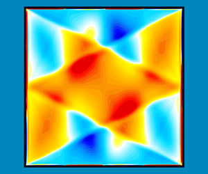
Figure 1. Schematic of the stably stratified square cavity under harmonic horizontal forcing, together with the effective gravity vector relative to the oscillating cavity,  $\boldsymbol {\xi }$. The inset is a snapshot at maximal phase of the vorticity, $\eta$, at buoyancy number $R_N={10^6}$, Prandtl number $Pr=1$, aspect ratio ${A{\kern-4pt}R} =1$, squared forcing frequency $\omega ^2=1/5$ and forcing amplitude $\alpha ={0.01}$.
Under the Boussinesq approximation, the non-dimensional governing equations are
 \begin{equation} \left.\begin{array}{c@{}} (\partial_t + \boldsymbol{u}\boldsymbol{\cdot}\boldsymbol{\nabla})\boldsymbol{u} ={-}{\boldsymbol{\nabla}} p + \dfrac{1}{R_N}{\nabla}^2 \boldsymbol{u} - T\boldsymbol{\xi},\quad \boldsymbol{\nabla}\boldsymbol{\cdot} \boldsymbol{u} = 0,\\ (\partial_t + \boldsymbol{u}\boldsymbol{\cdot}\boldsymbol{\nabla}) T = \dfrac{1}{PrR_N}{\nabla}^2 T, \end{array}\right\} \end{equation}
where  $p$ is the reduced pressure, the buoyancy number $R_N = NL^2/\nu$ is the ratio of the viscous and buoyancy time scales (it is the square root of the Grashof number) and $Pr = \nu /\kappa$ is the Prandtl number.
The governing equations (2.1) are solved numerically using a spectral-collocation method; the solutions are referred to as direct numerical simulations (DNS). The numerical technique used is the same as was used in Wu, Welfert & Lopez (Reference Wu, Welfert and Lopez2018), Yalim et al. (Reference Yalim, Welfert and Lopez2019b) and Grayer et al. (Reference Grayer, Yalim, Welfert and Lopez2020, Reference Grayer, Yalim, Welfert and Lopez2021). Briefly, the velocity, pressure and temperature are approximated by polynomials of up to degree  $280$, associated with the Chebyshev–Gauss–Lobatto grid. A fractional-step improved projection method, based on a linearly implicit and stiffly stable second-order-accurate scheme, is used to integrate in time. The temporal resolution used was 1800 time steps per forcing period; this is far more than needed for numerical stability and accuracy, and was selected for the improved analysis of the contributions from the higher temporal harmonics.
Although the system is solved in terms of the velocity, temperature and pressure, it is convenient to present the results in terms of the vorticity, whose only non-zero component is
 \begin{equation} \eta=\partial_z u -\partial_x w, \end{equation}
and the temperature deviation away from linear stratification
 \begin{equation} \theta=T-z. \end{equation}
 When the system is subjected to small periodic horizontal oscillations of amplitude  $\alpha$, the response flow is a synchronous limit cycle with discrete time invariance
 \begin{equation} \mathcal{T}:[\eta,\theta](x,z,t)\mapsto[\eta,\theta](x,z,t+2{\rm \pi}/\omega), \end{equation}
and centrosymmetry (invariance to a reflection through the origin)
 \begin{equation} \mathcal{C}:[\eta,\theta](x,z,t)\mapsto[\eta,-\theta]({-}x,-z,t). \end{equation}
The symmetry  $\mathcal {C}$ is the composition, $\mathcal {C}=\mathcal {H}_x\mathcal {H}_z=\mathcal {H}_z\mathcal {H}_x$, of two half-period flip space–time symmetries of the forced problem, $\mathcal {H}_x$ and $\mathcal {H}_z$. The actions of $\mathcal {H}_x$ and $\mathcal {H}_z$ are
 \begin{equation} \left.\begin{array}{c@{}} \mathcal{H}_x:[\eta,\theta](x,z,t)\mapsto[-\eta, \theta] ({-}x, z,t+{\rm \pi}/\omega),\\ \mathcal{H}_z:[\eta,\theta](x,z,t)\mapsto[-\eta,-\theta] ( x,-z,t-{\rm \pi}/\omega). \end{array}\right\} \end{equation}
For synchronous response flows that are harmonic in time, the space–time symmetries  $\mathcal {H}_x$ and $\mathcal {H}_z$ imply that $\eta$ is even in both $x$ and $z$, while $\theta$ is odd in $x$ and even in $z$. Limit cycles that are not pointwise invariant (centrosymmetric at every instant in time) may instead be setwise invariant, whereby they are invariant to a spatio-temporal symmetry consisting of $\mathcal {C}$ composed with a half-period translation in time. The action of this spatio-temporal symmetry is
 \begin{equation} \mathcal{C}_\textrm{ST}:[\eta,\theta](x,z,t)\mapsto [\eta,-\theta]({-}x,-z,t+{\rm \pi}/\omega). \end{equation}
The degree to which a state has broken centrosymmetry is quantified by an asymmetry parameter, based on the state's temperature field,  $T$:
$T$:
 \begin{equation} \mathcal{A} = \frac{\| T - \mathcal{C}\,T\|}{\| T \|}, \quad\text{where } \|({\boldsymbol{\cdot}})\|=\sqrt{\int_{{-}0.5}^{0.5}\int_{{-}0.5}^{0.5} ({\boldsymbol{\cdot}})^2\, {{\rm d}\kern0.06em x}\, {\rm d} z}. \end{equation}
 The dynamical behaviour of the field  $q=\eta$ or $\theta$ of the response flow may be examined by expanding $q$ as a Fourier series:
 \begin{equation} q(x,z,t) = q_0(x,z) + \sum_{k=1}^\infty q_k(x,z) \cos(k\omega t-\phi_k), \end{equation}
with coefficients
 \begin{align} q_0(x,z) = \frac{1}{\tau} \int_0^\tau q(x,z,t)\, {\rm d} t, \quad q_k(x,z) = \frac{2}{\tau} \int_0^\tau q(x,z,t)\cos(k\omega t-\phi_k)\, {\rm d} t, \ k>0, \end{align}
where  $\tau$ is a time length and the phase $\phi _k$ is optimized to maximize $\|q_k\|$ for each $k>0$ (see Appendix C for details). For synchronous responses, $\tau =2{\rm \pi} /\omega$ is the forcing period. For quasi-periodic or aperiodic responses, $q$ is detrended and Blackman windowed before (2.10a,b) is applied with $\tau = 2{\rm \pi} n_\tau /\omega$, using a number $n_\tau \approx k\omega /\omega _i$ of forcing periods for filtering at a frequency $\omega _i$. The values of $n_\tau$ used range from $n_\tau \ge 10$ for extracting the Fourier coefficients $q_k(x,z)$ from asynchronous responses to $n_\tau =20\,000$ for computing power spectral densities (PSDs).
3. Nonlinear responses to moderate-amplitude forcing
As mentioned in the Introduction, the analysis in Grayer et al. (Reference Grayer, Yalim, Welfert and Lopez2021) for  ${A{\kern-4pt}R} =1$ showed that for very small forcing amplitudes $\alpha$, and sufficiently large $R_N$, the response to horizontal oscillations of the container with frequency $\omega$ comes in two flavours, codified in terms of a Fredholm alternative, depending on whether or not $\omega$ resonates with the frequency of a Thorpe mode. The $m{\,:\,}n$ Thorpe mode has frequency
 \begin{equation} \sigma_{m{\,:\,}n}=\frac{1}{\sqrt{1+n^2/m^2}}\in(0,1) \end{equation}
for integers  $m$ and $n$; all of its spatial harmonics (the $km{\,:\,}kn$ Thorpe modes) have the same frequency. For forcing frequencies in the range $0<\omega <1$, we can write $\omega ^2=1/(1+r^2)\in (0,1)$ with $r$ any positive real number. For forcing frequencies corresponding to irrational $r$, or rational $r=n/m$ with positive integers $m$ and $n$ of opposite parities, there is a forced response which is synchronous with the forcing and invariant to the symmetries of the forced system at that frequency (Fredholm alternative A1). On the other hand (Fredholm alternative A2), $r=n/m$ with integers $m$ and $n$ both odd results in a response in resonance with Thorpe modes for which $\sigma ^2_{m\,:\,n}\approx \omega ^2$, the approximation being due to viscous effects.
In this paper, we consider in detail the forced responses at
 \begin{equation} \omega=1/\sqrt{5} \approx 0.4472, \end{equation}
for which the second temporal harmonic is inside the range of frequencies of the Thorpe modes, i.e.  $2\omega <1$. These are computed for
 \begin{equation} {A{\kern-4pt}R}=1, \quad Pr=1 \quad \text{and}\quad R_N={10^6}. \end{equation}
This  $R_N$ was found to be sufficiently large to produce responses that are not dominated by viscous damping, and for forcing amplitudes ranging from $\alpha ={10^{-6}}$ up to and beyond the levels where the symmetric synchronous response flow loses stability. In laboratory experiments using salt as the stratifying agent, the buoyancy frequency is limited to $N \approx 0.6\ \textrm {rad}\ \textrm {s}^{-1}$, the depth of the fluid to $L\sim 1$ m and the kinematic viscosity is $\nu \sim 10^{-6}\ \textrm {m}^2\ \textrm {s}^{-1}$, giving $R_N\sim 6\times 10^{5}$ (Savaro et al. Reference Savaro, Campagne, Linares, Augier, Sommeria, Valran, Viboud and Mordant2020). The contributions of the temporal harmonics to the structure of the forced response flow become more important with increasing $\alpha$. Those contributions arise from the interactions between the primary response and the parametric forcing, $T\boldsymbol {\xi }(t)$, as well as the nonlinear advection terms, $(\boldsymbol {u}\boldsymbol {\cdot }\boldsymbol {\nabla })\boldsymbol {u}$ and $(\boldsymbol {u}\boldsymbol {\cdot }\boldsymbol {\nabla })T$.
3.1. Forced symmetric synchronous responses at small  $\alpha$

We begin by considering sufficiently small forcing amplitudes  $\alpha$, for which the response flow is synchronous with the forcing. The phase of the forced response flow is as expected; the vorticity $\eta$ response is maximal at the zero phase of the forcing and the temperature deviation $\theta$ response is maximal a quarter period later. Figure 2 shows snapshots of $\eta$ and $\theta$ for forcing amplitudes $\alpha \in [{10^{-6}},0.026]$. At the lowest $\alpha ={10^{-6}}$, the response flow is that reported in Grayer et al. (Reference Grayer, Yalim, Welfert and Lopez2021) with essentially piecewise-constant vorticity (viscously regularized), corresponding to a 1 : 2 harlequin response. Appendix A gives the explicit analytical expressions for this forced response at $\omega =1/\sqrt {5}$ in the linear inviscid limits, $R_N\to \infty$ and $\alpha \to 0$.
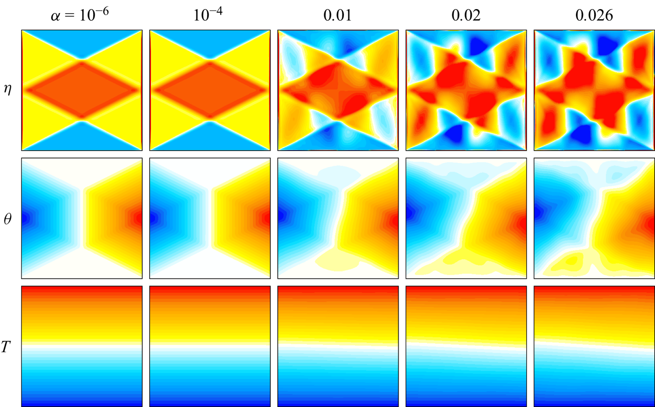
Figure 2. Snapshots of the vorticity  $\eta$, temperature deviation $\theta$ and isotherms $T$ of the response flows at $\alpha$ as indicated, shown at forcing phases 0 for $\eta$ and ${\rm \pi} /2$ for $\theta$ and $T$. The contour level bounds are $\eta =\pm 4\alpha$, $\theta =\pm 1.2\alpha$ and $T=\pm 0.5$, with blue negative and red positive.
For the forcing frequency considered,  $\omega =1/\sqrt {5}$, the characteristics retrace, going from a corner on one sidewall to the middle of the opposite sidewall, back to the other corner on the original sidewall, and then back again. These characteristic lines demarcate regions of nearly constant vorticity. The (scaled) vorticity of the response flow at $\alpha ={10^{-4}}$ is visually very similar, but at $\alpha =0.01$ regions demarcated by the characteristics are no longer of nearly constant vorticity. A cellular pattern with four cells horizontally and two vertically, reminiscent of the 4 : 2 Thorpe mode, appears. At $\alpha \gtrsim 0.02$, these cells are prominent, but distorted along characteristics associated with the forcing frequency $\omega$, as well as along characteristics associated with the second harmonic of the forcing frequency, $2\omega$. This all suggests that the temporal second harmonic of the response flow is becoming dynamically important.
Figure 3 shows how  $\|\eta _k\|$ and $\|\theta _k\|$ for $k=0$, 1 and 2 vary with forcing amplitude $\alpha$. For $\alpha ={10^{-6}}$, all $\|\eta _k\|$ and $\|\theta _k\|$ other than for $k=1$ are essentially machine noise, with optimal phases $\phi _1\approx 0$ for $\eta$ and $\phi _1\approx {\rm \pi}/2$ for $\theta$, confirming that the forced response is essentially the $1{\,:\,}2$ harmonic standing wave harlequin pattern described in Grayer et al. (Reference Grayer, Yalim, Welfert and Lopez2021). In the range $\alpha \in [{10^{-6}},0.01]$, the norms scale with $\alpha ^k$ for $k>0$, whereas the temporal means, $\|\eta _0\|$ and $\|\theta _0\|$, scale with $\alpha ^2$, as is expected for a mean flow arising from quadratic nonlinear interactions in the synchronous response. By $\alpha \approx 0.01$, the second harmonics $\|\eta _2\|$ and $\|\theta _2\|$ have grown to just less than an order of magnitude smaller than the respective first harmonics, $\|\eta _1\|$ and $\|\theta _1\|$, resulting in the nonlinear distortions to the $\eta$ harlequin pattern and isotherms that are not horizontal. The growth of the second harmonic with $\alpha ^2$ slightly shifts the optimal phases of $\eta _1$ and $\theta _1$ from $0$ and $0.5{\rm \pi}$ at low $\alpha$ to approximately $-0.007{\rm \pi}$ and $0.501{\rm \pi}$ at $\alpha =0.026$.
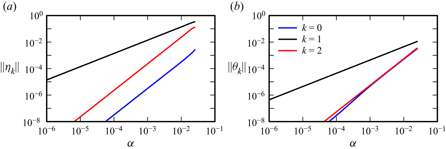
Figure 3. Variation with  $\alpha$ of the leading Fourier coefficient magnitudes, (a) $\|\eta _k\|$ and (b) $\|\theta _k\|$, for $k=0$, 1 and 2.
Figure 4 shows the Fourier coefficients of  $\eta$ and $\theta$ for $k=0$, $1$ and $2$ for various values of $\alpha$. For these symmetric synchronous response flows, the space–time symmetries $\mathcal {H}_x$ and $\mathcal {H}_z$ imply that the Fourier coefficients of $\eta$ and $\theta$ have the following spatial symmetries: $\eta _k$ is odd (even) in both $x$ and $z$ and $\theta _k$ is even (odd) in $x$ and odd (even) in $z$ for $k$ even (odd), which they do.
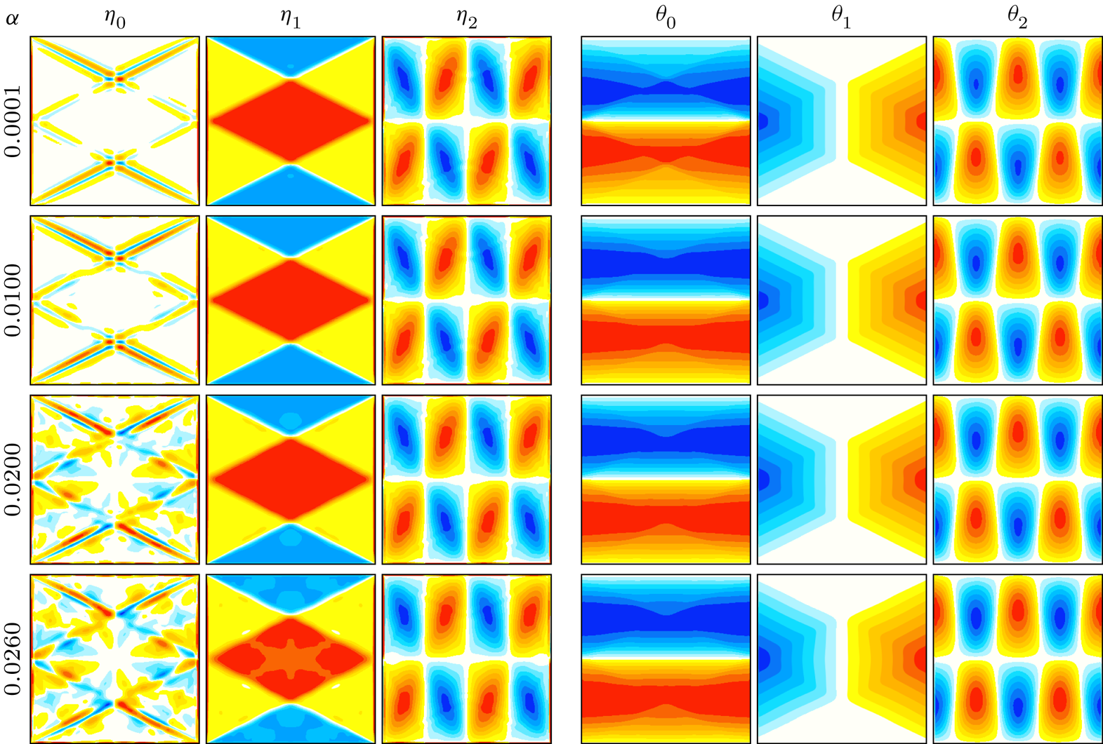
Figure 4. Fourier coefficients of  $\eta _k$ and $\theta _k$, $k=0,1,2$, obtained from DNS via filtering at frequencies $0$,
$0$,  $\omega$ and $2\omega$ with maximal phase $\phi _k$, at $\alpha$ as indicated. The fields are scaled by the maximum in $(x,z)\in [-0.45,0.45]^2$ for $\eta$ and in the whole square for $\theta$. Supplementary movie 1 animates, over one forcing period, $\eta$, $\theta$ and $T$ from the DNS (figure 2) along with their Fourier reconstructions using $k=0$, 1 and 2 for $\alpha =0.026$.
The  $\eta$ mean flow is very weak, with $\|\eta _0\|$ being two orders of magnitude smaller than $\|\eta _2\|$ (see figure 3a). At low $\alpha$, the structure of $\eta _0$ consists of thin boundary layers along with thin vortex sheets emitted from the four corners of the container. These shear layers are aligned with the characteristics for $\omega$. For $\alpha \gtrsim 0.02$, additional structures are evident in $\eta _0$, which correspond to weaker and broader shear layers emitted at the midpoints of the sidewalls, where the shear layers along the $\omega$ characteristics reflect. These weaker shear layers are aligned with the characteristics for $2\omega$. In contrast, $\|\theta _0\|$ and $\|\theta _2\|$ are of the same order. The structure of $\theta _0$ is essentially invariant with $\alpha$, showing no discernible influence of the second harmonic. Appendix B shows that in the linear inviscid limit, the mean $\eta$ is zero but the mean $\theta$ is non-zero.
Supplementary movie 1, available at https://doi.org/10.1017/jfm.2023.618, animates  $\eta$, $\theta$ and $T$ from the DNS over one forcing period for $\alpha =0.026$, along with their truncated Fourier reconstructions (2.9) using only $k=0$, 1 and 2. There is no discernible difference between the DNS and its truncated Fourier reconstruction. The movie shows that in both the DNS and its Fourier reconstruction, characteristics associated with the frequency $2\omega$ are being emitted at the midpoints of the sidewalls, where the characteristics associated with the forcing frequency $\omega$ reflect, as evident in the $k=2$ Fourier coefficient $\eta _2$. The generation of second-harmonic wavebeams at locations where wavebeams reflect at walls inclined to the gravity vector has drawn considerable attention (Peacock & Tabaei Reference Peacock and Tabaei2005; Tabaei, Akylas & Lamb Reference Tabaei, Akylas and Lamb2005; Rodenborn et al. Reference Rodenborn, Kiefer, Zhang and Swinney2011). Here, the walls become increasingly oblique to the effective gravity vector $\boldsymbol {\xi }(t)$ as the horizontal forcing amplitude $\alpha$ is increased. The angle between the effective gravity vector and the vertical walls is $\arcsin (\alpha \sin \omega t)$.
The  $4{\,:\,}2$ regular cellular structures are clearly evident in the Fourier components $\eta _2$ and $\theta _2$. These second-harmonic Fourier components oscillate at a frequency corresponding to $(2\omega )^2=4/5=1/(1+r^2)$, for which $r=n/m=1/2=2/4$. The association with the $4{\,:\,}2$ Thorpe mode, rather than the $2{\,:\,}1$ Thorpe mode, is a consequence of the space–time symmetry constraints noted earlier, which imply that the second-harmonic vorticity Fourier coefficients must be odd functions of both $x$ and $z$ while for the temperature deviation they must be odd in $x$ and even in $z$; the $2{\,:\,}1$ Thorpe mode does not satisfy these symmetry constraints whereas its spatial harmonic, the $4{\,:\,}2$ Thorpe mode, does. The emergence of the $4{\,:\,}2$ Thorpe mode is not an instability, but rather a superharmonic resonance. It is present even as $\alpha \to 0$, and the forced response flow is a symmetric synchronous limit cycle that is not temporally harmonic.
3.2. Triadic instabilities of the forced response as $\alpha$ is increased

As  $\alpha$ is increased beyond a critical value, $\alpha _1\approx 0.0261$, the symmetric synchronous response loses stability via a supercritical bifurcation that both breaks the centrosymmetry $\mathcal {C}$ and introduces an additional frequency which is nearly commensurate with $\omega$. The resulting two-frequency quasi-periodic flow is not setwise $\mathcal {C}$ invariant; applying $\mathcal {C}$ results in a slightly different quasi-periodic flow. With further increases in $\alpha$, additional instabilities occur. Figure 5 is a bifurcation diagram showing how the time-averaged asymmetry parameter $\langle \mathcal {A}\rangle$ varies with $\alpha$. The time average is taken over $n_\tau =10\,000$ forcing periods as the responses are increasingly temporally complicated for $\alpha >\alpha _1$. The different states resulting from the sequence of instabilities are colour-coded. The blue curve corresponds to the symmetric synchronous limit cycle forced response described in § 3.1, the red curve corresponds to a symmetry-broken quasi-periodic state with two incommensurate frequencies, the green curve corresponds to another quasi-periodic state with three incommensurate frequencies and the cyan curve corresponds to states with additional temporal complexity. Each of these states and the instabilities from which they stem are described in detail below.
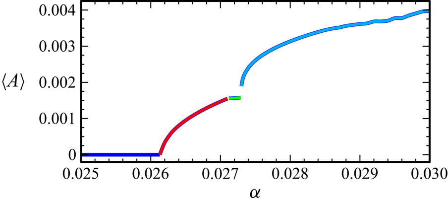
Figure 5. Bifurcation diagram showing how the time-averaged asymmetry parameter  $\langle \mathcal {A}\rangle$ varies with $\alpha$.
The PSDs obtained from time series of the temperature at a collocation point,  $T(1/\sqrt {8},1/\sqrt {8},t)$, consisting of $n_\tau =20\,000$ forcing periods sampled at a rate of 100 per forcing period, taken long after initial transients have died off (typically after 80 000 forcing periods), are shown in figure 6 for a selection of $\alpha$. The PSD in figure 6(a) is of the symmetric synchronous response at $\alpha =0.026$ and consists of a peak at the forcing frequency $\omega$ and its superharmonics; the PSDs are only shown for frequencies $f\in [0,1.2]$, extending a little beyond the range of frequencies of the Thorpe modes. The second harmonic, $2\omega$, is labelled as $\omega _1$, plays a fundamental role as $\alpha$ is increased. As described in the previous subsection, Fourier filtering at $\omega _1$ reveals the $4{\,:\,}2$ Thorpe mode, which is now labelled ${M}_1$.
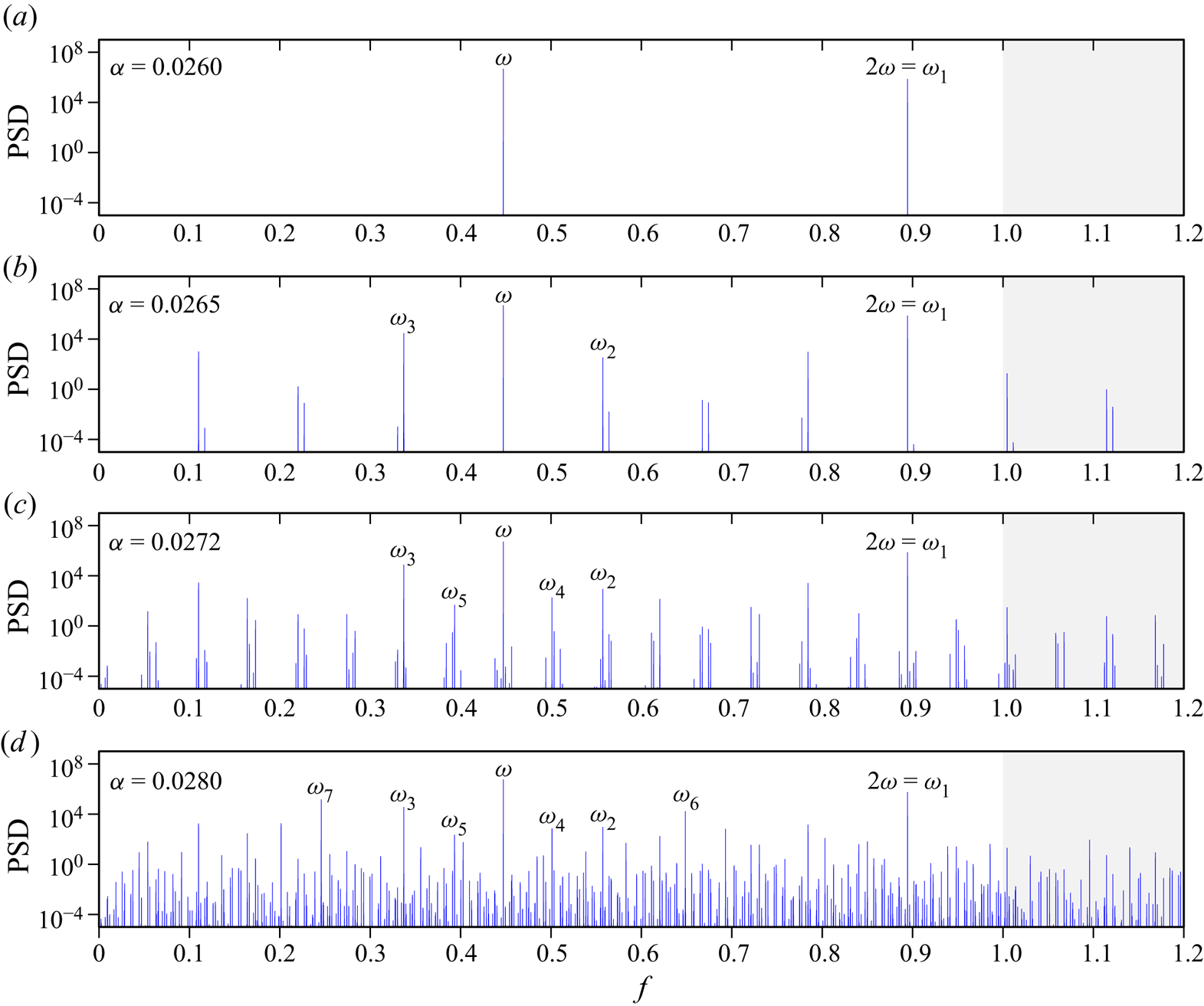
Figure 6. The PSDs of the temperature at a point,  $T(1/\sqrt {8},1/\sqrt {8},t)$, for $\alpha$ as indicated. The PSDs were determined from time series of $n_\tau =20\,000$ forcing periods taken well after initial transients have died off (typically after 80 000 forcing periods).
For  $\alpha =0.02650>\alpha _1$, the PSD in figure 6(b) consists of additional peaks. All of these correspond to linear combinations of $\omega$ and any other peak other than a harmonic of $\omega$. Fourier filtering at each of these peaks with $\textrm {PSD}>1$ only reveals coherent structures for some frequencies, namely $\omega$, $\omega _1=2\omega$ and two other frequencies labelled $\omega _2$ and $\omega _3$. The Fourier coefficient at $\omega _2\approx 0.5573$ is strongly correlated with the Thorpe mode ${M}_2=10{\,:\,}15$ with $\sigma _{10{\,:\,}15}\approx 0.5547$, and that at $\omega _3\approx 0.3371$ with the Thorpe mode ${M}_3=6{\,:\,}17$ with $\sigma _{6{\,:\,}17}\approx 0.3328$. These Fourier coefficients are shown in figure 7. As ${M}_2$ and ${M}_3$ have $m$ and $n$ of opposite parities, the centrosymmetry $\mathcal {C}$ is broken. The three modes ${M}_1$, ${M}_2$ and ${M}_3$ exactly satisfy the spatial conditions on wavevectors for triadic resonance (Thorpe Reference Thorpe1966), namely $4=10-6$ and $2=-15-(-17)$, i.e. ${M}_1=\bar {{M}}_2-\bar {{M}}_3$, where $\bar {{M}}=m{\,:\,}-n$ is the conjugate of ${M}=m{\,:\,}n$. While the response frequencies exactly satisfy $\omega _1=2/\sqrt {5}=\omega _2+\omega _3$, the modes ${M}_1$, ${M}_2$ and ${M}_3$ only approximately satisfy the inviscid frequency condition for triadic resonance, and have a detuning
 \begin{align} \delta\sigma_1:=\sigma_{4{\,:\,}2}-\sigma_{10{\,:\,}({-}15)} -\sigma_{({-}6){\,:\,}17} =\frac{2}{\sqrt{5}}-\frac{10}{\sqrt{325}}-\frac{6}{\sqrt{325}} =\frac{2}{\sqrt{5}}\left[1-\frac{8}{\sqrt{65}}\right] \approx 0.0069. \end{align}
The PSD in figure 6(b) shows that  $\omega _3$ and $\omega$ are nearly commensurate in a ratio 3 to 4 or, equivalently, the first peak at $\omega -\omega _3$ is nearly a quarter of $\omega$. The small detuning
 \begin{equation} \delta\omega_1=\omega-4(\omega-\omega_3)=4\omega_3-3\omega \approx 0.0068 \end{equation}
manifests as sidebands of lower power to the main peaks in the PSD and as a beat frequency in the corresponding time series, corresponding to a beat period of  $\omega /\delta \omega _1\approx 66$ forcing periods. The near-perfect match between $\delta \omega _1$ in (3.5) and $\delta \sigma _1$ in (3.4) is not entirely coincidental. It results from the ratio between individual detunings $\omega _2-\sigma _{10{\,:\,}15} \approx 0.0026$ and $\omega _3-\sigma _{6{\,:\,}17} \approx 0.0043$, approximately $3/5$, being nearly inverse to that, $5/3$, between $\sigma _{10{\,:\,}15}$ and $\sigma _{6{\,:\,}17}$; see Appendix D for a justification.
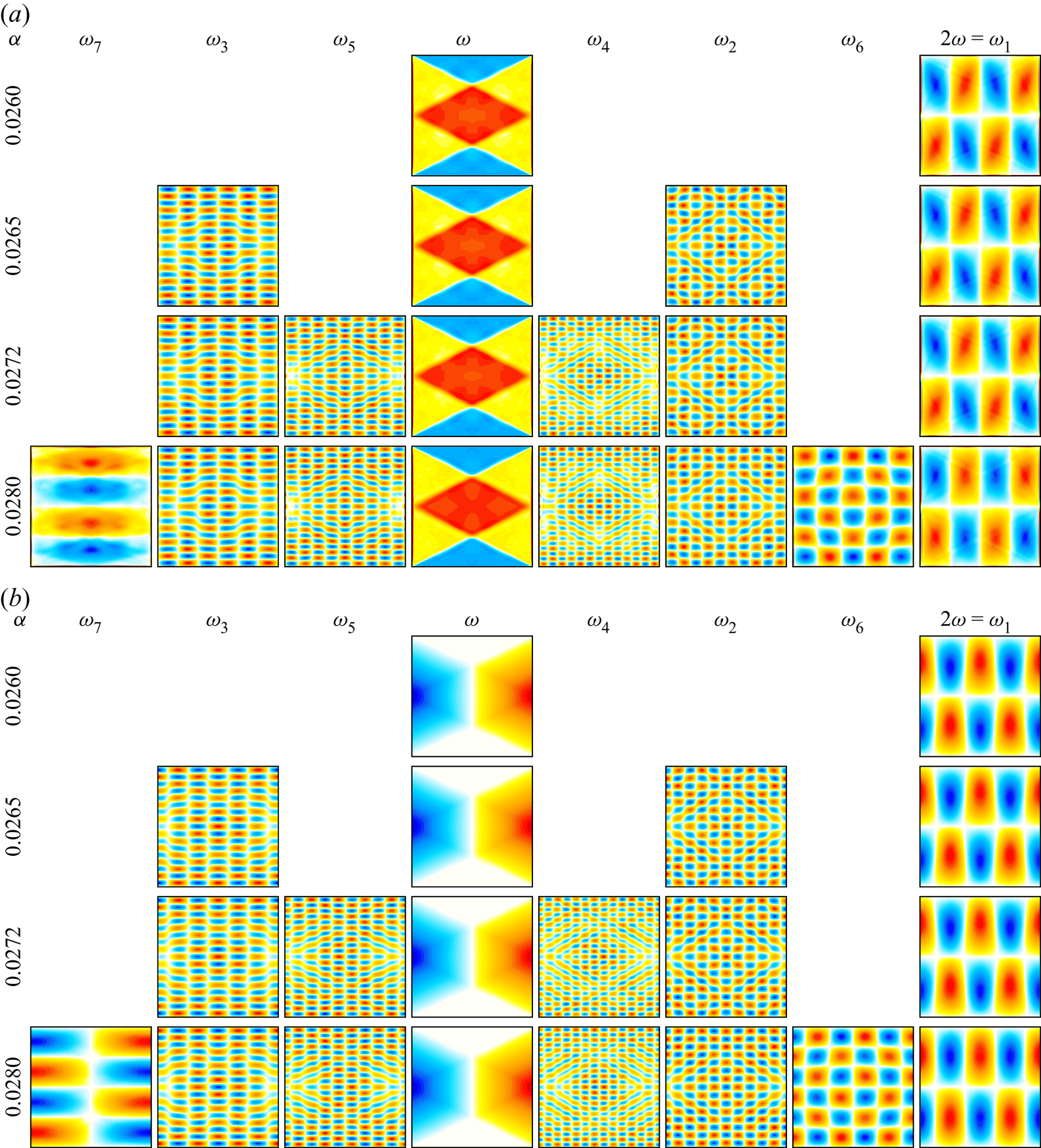
Figure 7. Responses  $\eta$ (a) and $\theta$ (b) filtered at the indicated frequencies for the indicated $\alpha$.
At  $\alpha =\alpha _2\approx 0.02711$, there is another supercritical instability that introduces another nearly commensurate frequency. The response is a three-torus, a flow state with three incommensurate frequencies (Lopez & Marques Reference Lopez and Marques2000, Reference Lopez and Marques2003). Figure 6(c) shows the PSD of this solution branch at $\alpha =0.0272$, consisting of all the peaks from the previous two-torus branch plus two additional frequencies, labelled $\omega _4$ and $\omega _5$, and linear combinations between all of these. The new frequencies $\omega _4\approx 0.5011$ and $\omega _5\approx 0.3934$ are also in exact triadic resonance with $\omega _1=\omega _4+\omega _5$. These frequencies are close to those of Thorpe modes ${M}_4=13{\,:\,}23$ with $\sigma _{13{\,:\,}23}\approx 0.4921$ and ${M}_5=9{\,:\,}21$ with $\sigma _{9{\,:\,}21}\approx 0.3939$. The Fourier coefficients at $\omega _4$ and $\omega _5$ for $\alpha =0.0272$ are shown in figure 7, along with those of $\omega$, $\omega _1$, $\omega _2$ and $\omega _3$ which remain essentially unchanged from the two-torus branch at lower $\alpha$. The wavevectors of ${M}_1$, ${M}_4$ and ${M}_5$ also are in exact triadic resonance, $4=13-9$ and $2=23-21$, i.e. ${M}_1={M}_4-{M}_5$. So, the three-torus branch consists of two sibling triadics spawned from the same parent mode. The Thorpe modes ${M}_4$ and ${M}_5$ have $m$ and $n$ of the same parity and the three-torus branch recovers setwise $\mathcal {C}$ invariance but continues to have broken pointwise $\mathcal {C}$ symmetry. This very likely accounts for $\langle \mathcal {A}\rangle$ being nearly constant along this branch (the green curve in the bifurcation diagram of figure 5). With $\omega _5\approx (\omega _3+\omega )/2$, an additional small detuning $\delta \omega _2 = 2\omega _5-(\omega _3+\omega )\approx {0.0025}$ is introduced. The relation $\delta \omega _1\approx 3\delta \omega _2$ introduces an even smaller detuning $\delta \omega _3=3\delta \omega _2-\delta \omega _1 =6\omega _5-7\omega _3\approx {0.0007}$ and a longer beat period $\omega /\delta _3\approx 640$ forcing periods. However, this beat is much weaker than the dominant beat of ${66}$ forcing periods.
At  $\alpha =\alpha _3\approx 0.02735$, the three-torus solution branch becomes unstable as yet another weakly incommensurate frequency is introduced in the bifurcated state, whose time-averaged asymmetry parameter $\langle \mathcal {A}\rangle$ increases rapidly with small increases in $\alpha$. The PSD of this solution branch at $\alpha =0.0280$ shown in figure 6(d) consists of all the frequency peaks identified in the earlier branches, plus two new frequency peaks at $\omega _6\approx 0.6486$ and $\omega _7\approx 0.2458$, which are also in exact triadic resonance with $\omega _1=\omega _6+\omega _7$. These frequencies are close to those of Thorpe modes ${M}_6=5{\,:\,}6$ with $\sigma _{5{\,:\,}6}\approx 0.6402$ and ${M}_7=1{\,:\,}4$ with $\sigma _{1{\,:\,}4}\approx 0.2425$. There are many other peaks in the PSD which are readily identified as linear combinations of $\omega$, $\omega _3$, $\omega _5$ and $\omega _7$. The Fourier coefficients of $\omega$ and $\omega _i$, $i=1,\ldots,7$, are shown in figure 7; the Fourier coefficients at the frequency peaks that existed in the three-torus branch remain essentially the same, and the Fourier coefficients of $\omega _6$ and $\omega _7$ have wavevectors corresponding to those of ${M}_6$ and ${M}_7$, which are also in exact triadic resonance with ${M}_1={M}_6-{M}_7$; $4=5-1$ and $2=6-4$. Modes ${M}_6$ and ${M}_7$ have $m$ and $n$ of opposite parities, contributing to the rise in $\langle \mathcal {A}\rangle$ shown in figure 5. The new modes introduce a new small detuning $\delta \omega _4=5\omega _5-8\omega _7\approx {0.0004}$, associated with a longer beat period of $\omega /\delta \omega _4\approx {1100}$ forcing periods. Over the range of $\alpha$ considered, the spatial structures of the means $\eta _0$ and $\theta _0$ remain essentially the same as those of the synchronous symmetric limit cycle at $\alpha \sim 0.02$ shown in figure 4. This is not too surprising as the means are dominated by the Fourier coefficients with largest power, which are those at $\omega$ and $2\omega$.
Figure 8 and table 1 summarize the resonances of the three triads  $({M}_1,\bar {{M}}_2,-\bar {{M}}_3)$, $({M}_1,{M}_4,-{M}_5)$ and $({M}_1,{M}_6,-{M}_7)$, in both frequency and wavevectors. Figure 8(a) shows a contour plot of the detuning
 \begin{align} \delta\sigma_{m{\,:\,}n} :=\sigma_{4{\,:\,}2}-\sigma_{m{\,:\,}n}-\sigma_{(4-m){\,:\,}(2-n)} =\frac{2}{\sqrt{5}}-\frac{|m|}{\sqrt{m^2+n^2}}- \frac{|4-m|}{\sqrt{(4-m)^2+(2-n)^2}} \end{align}
as a function of the horizontal and vertical wavenumbers,  $m$ and $n$, together with thick dark blue curves of the zero contour level, corresponding to an exact (inviscid) triadic resonance between the parent mode ${M}_1=4{\,:\,}2$ and a pair of offspring modes $m{\,:\,}n$ and $(4-m){\,:\,}(2-n)$. The expression (3.6) generalizes (3.4), with $\delta \sigma _1=\delta \sigma _{10{\,:\,}-15}=\delta \sigma _{(-6){\,:\,}17}$ for $m{\,:\,}n=10{\,:\,}(-15)=\bar {{M}}_2$ or $m{\,:\,}n=(-6){\,:\,}17=-\bar {{M}}_3$. The symmetry $\delta \sigma _{m{\,:\,}n}=\delta \sigma _{(4-m){\,:\,}(2-n)}$ is reflected by the symmetry of the contours about the point $(m,n)=(2,1)$, marked with a crosshair $+$. The two offspring modes of all triads are symmetrically located with respect to that point. The parent mode ${M}_1$, from which all triads spawn, is symmetric to the origin at $(m,n)=(0,0)$, associated with the mean flow ${M}_0=0{\,:\,}0$. Figure 8(b) shows that the wavevectors of each of the offspring modes in the triads add up exactly to that of the parent mode, forming triangles. Those offspring modes, however, do not fall exactly on the zero contour curve of $\delta \sigma _{m{\,:\,}n}$, giving the respective small detunings in frequencies. For each of the triads, these resonances can be made exact in frequencies by slightly adjusting the aspect ratio of the container, but the adjustment would be different for each triad. For example, changing the container aspect ratio from ${A{\kern-4pt}R} =1$ to ${A{\kern-4pt}R} =0.9899$ would make $\delta \sigma _1=0$.
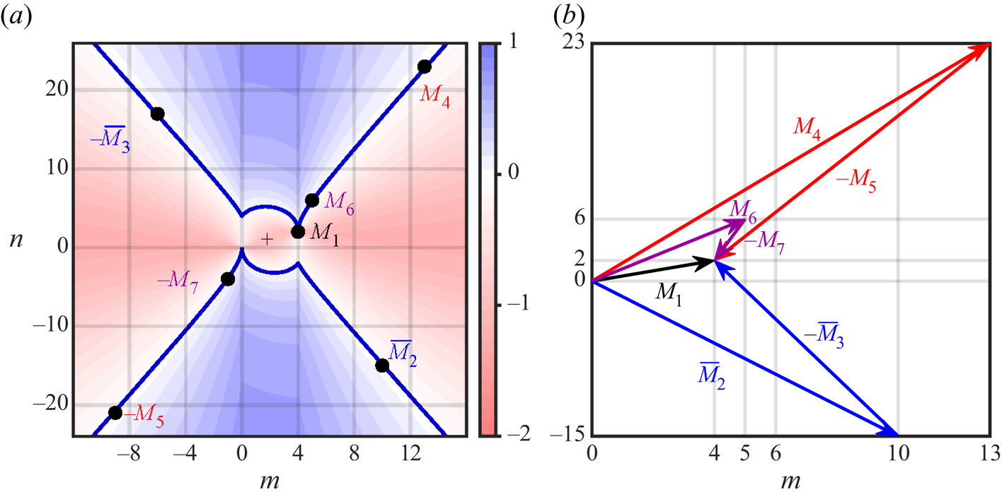
Figure 8. Triadic resonances from  ${M}_1$. (a) Contour plot of $\delta \sigma _{m{\,:\,}n}$ (3.6) as a function of wavenumbers $m$ and $n$. The crosshair $+$ marks the centre of symmetry. Triadic modes are (approximately) on the zero-level contours (dark blue curves). (b) Wavevectors associated with the triads ${M}_1=\bar {{M}}_2-\bar {{M}}_3= {M}_4-{M}_5= {M}_6-{M}_7$.
Table 1. Response frequencies  $\omega _i$, natural frequencies $\sigma _i$ and detunings of the modes involved in the triadic resonances observed in the range $\alpha \in [0.026,0.030]$. The positive combined detunings in the last column imply that all triadic siblings are located in the blue area in figure 8(a).

Which offspring modes are first spawned in a triad triggered by a parent mode associated with a resonant superharmonic response is in general unclear. In the case studied here, the primary forced response has vorticity consisting of a harlequin pattern which is piecewise-constant, generated by the  $1{\,:\,}2$ Thorpe mode and its odd spatial harmonics. The second temporal harmonic is a resonant response dominated by the Thorpe mode ${M}_1=2(2{\,:\,}1)=4{\,:\,}2$ that grows with the square of the amplitude of the forcing, $\alpha ^2$, until its enstrophy approaches the enstrophy level of the primary response. Then, the synchronous limit cycle loses stability via triadic resonance. The offspring modes in the three triadic resonances that are successively excited as $\alpha$ is further increased are of the form
 \begin{equation} m{\,:\,}n=(2{\,:\,}1)\pm(k{\,:\,}\ell), \end{equation}
with  $k{\,:\,}\ell =\overline {8{\,:\,}16}=8(\overline {1{\,:\,}2})$, $k{\,:\,}\ell =11{\,:\,}22=11(1{\,:\,}2)$ and $k{\,:\,}\ell =3{\,:\,}5$, respectively. While these have increasing magnitudes of detuning $\delta \sigma _1\approx 0.0069$, $\delta \sigma _2\approx 0.0085$ and $\delta \sigma _3\approx 0.0117$, other factors may also be contributing to the selection process.
One possible factor in the weakly viscous setting is the size of the wavenumbers  $m$ and $n$ of the offspring modes contributing to their viscous damping. For example, the modes $\bar {{M}}_2$ and $-\bar {{M}}_3$ belong to the family of mode pairs (3.7) with $\ell =-2k$ that are in approximate triadic resonance with ${M}_1=4{\,:\,}2$, with corresponding detuning
 \begin{equation} \delta\sigma_{(2+k){\,:\,}(1-2k)} =\frac{2}{\sqrt{5}}\left(1-\frac{k}{\sqrt{k^2+1}}\right) =\frac{\sigma_{4{\,:\,}2}}{\sqrt{k^2+1}\quad (k+\sqrt{k^2+1})}, \end{equation}
decreasing quadratically with  $k$. At $R_N={10^6}$, $k=8$ appears to be a compromise between small detuning (large $k$) and moderate dissipation (small $k$).
$k$).
The alignment of the wavevector  $k{\,:\,}\ell$ with the primary Thorpe mode $1{\,:\,}2$ or its conjugate $\overline {1{\,:\,}2}=1{\,:\,}-2$ also appears to play a role in the selection of the triadic modes. In particular, the candidate triad $1{\,:\,}5+\overline {3{\,:\,}3}={M}_1$, which has a relatively low detuning $\delta \sigma \approx -0.0088$ and low wavenumbers, has $k{\,:\,}\ell =\overline {1{\,:\,}4}$, but is demoted in favour of the triad ${M}_6-{M}_7={M}_1$, possibly because of an angle $\theta =\arccos (9/\sqrt {85})\approx {12.5}^{\circ }$ with $\overline {1{\,:\,}2}$, about three times that, $\arccos (13/\sqrt {170})\approx {4.4}^{\circ }$, between $3{\,:\,}5$ and $1{\,:\,}2$, thereby lowering the energy required to sustain modal wavevectors transverse to the characteristic lines, which act as barriers to modal deformations. In fact, the alignment of wavevectors figures prominently in the coefficients of standard reduced models of resonant triadic interactions, in the form of scaled areas of the triangles formed by the wavevectors in figure 8(b) (Hasselmann Reference Hasselmann1967; McEwan & Plumb Reference McEwan and Plumb1977; Bourget et al. Reference Bourget, Dauxois, Joubaud and Odier2013; Ha Reference Ha2021; Grayson, Dalziel & Lawrie Reference Grayson, Dalziel and Lawrie2022). This alignment favours modes on the ‘straight’ branches of the zero-contour plot in figure 8(a) and tends to promote parametric subharmonic instability conditions, with larger $k$ in (3.8) possible at larger $R_N$.
Another possible factor in the selection process is that the system favours positive detunings, which allow for the available energy, proportional to
 \begin{equation} \sigma_{4{\,:\,}2}^2>(\sigma_{m{\,:\,}n}+\sigma_{(4-n){\,:\,}(2-n)})^2 >\sigma_{m{\,:\,}n}^2+\sigma_{(4-m){\,:\,}(2-n)}^2, \end{equation}
to be distributed amongst the two offspring modes. The slight negative detuning of  $-{M}_5$ may partially explain the relative weakness, as measured by the intensity of the peaks in the PSD of figure 6, of the second triad compared with the other ones.
3.3. Very-low-frequency modulations
The third triadic resonance described in the previous subsection triggers a quasi-periodic response, essentially a four-torus at onset ( $\alpha \approx \alpha _3$), that is strongly influenced by the beat frequencies manifesting as sidebands. The new low-frequency beat $\delta \omega _4$ is relatively weak compared with the beat frequency $\delta \omega _1$ observed at lower $\alpha$ for $(\alpha -\alpha _3)/\alpha _3$ small. Its presence does not become fully apparent in the time series until $\alpha \gtrsim 0.0285$. This very-low-frequency (VLF) modulation regime is also apparent in the oscillations of $\langle \mathcal {A}\rangle$ for $\alpha \gtrsim 0.0285$ seen in the bifurcation diagram in figure 5. How this beat period $\tau _{VLF}=2{\rm \pi} /\delta \omega _4$ varies with $\alpha$ is shown in figure 9, and was measured from time series of $\mathcal {A}$, such as those shown in figure 10.
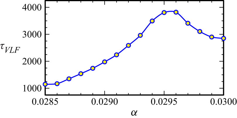
Figure 9. Variation of the VLF beat period  $\tau _{VLF}$ with $\alpha$.

Figure 10. (a–e) Time series of  $\mathcal {A}$ at $\alpha$ as indicated. The red highlighted region of the $\alpha =0.0290$ series corresponds to the time interval over which a rolling PSD analysis was conducted (see figure 13).
Very-low-frequency states may appear in autonomous (unforced) systems after a sequence of bifurcations introducing new frequencies into the flow (Lopez & Marques Reference Lopez and Marques2003; Abshagen et al. Reference Abshagen, Lopez, Marques and Pfister2005), but in the context of the present study, they have also been found to play important dynamical roles in parametrically forced flows, particularly in parameter regimes involving triadic resonances (Marques & Lopez Reference Marques and Lopez2015; Lopez & Marques Reference Lopez and Marques2016a,Reference Lopez and Marquesb, Reference Lopez and Marques2018).
To put a beat VLF period,  $\tau _{VLF}\sim {3600}$, into perspective, a typical laboratory experiment uses a buoyancy frequency $N\approx 0.6\ \textrm {rad}\ \textrm {s}^{-1}$, so the dimensional forcing period considered here is $2{\rm \pi} /(\omega N)= 2{\rm \pi} \sqrt {5}/0.6\approx 24$ s, resulting in a dimensional beat period ${3600}$ times longer, approximately one day.
The PSDs of the four cases in figure 10 are shown in figure 11. The PSD at  $\alpha =0.0285$ is very similar to that at $\alpha =0.0280$ shown in figure 6(d), except that the sidebands have slightly increased power. The PSD at the beat frequencies grows with $\alpha$, and so does the power in the superharmonics of the beat frequencies. This leads to sidebands that are broad Gaussians rather than discrete peaks. This becomes evident at $\alpha \approx 0.0285$ with the time series transitioning from a harmonically modulated signal to a distinctive slow–fast signal. By $\alpha =0.0290$, the power in the sidebands is considerably larger. More significant, however, is the decrease in power at frequencies $\omega _4$ and $\omega _5$ as $\alpha$ is further increased.

Figure 11. The PSDs of the temperature at a point,  $T(1/\sqrt {8},1/\sqrt {8},t)$, at $\alpha$ as indicated. The PSDs were determined for time series of 20 000 forcing periods long, well after initial transients have died off (after 80 000 forcing periods).
The Fourier coefficients at the frequencies  $\omega$ and $\omega _i$, $i=1,\ldots,7$, are shown in figure 12 at the same $\alpha$ values used for the PSDs in figure 11, illustrating that the Fourier coefficients at $\omega _4$ and $\omega _5$ (corresponding to the offspring modes in the second triadic) lose coherence for $\alpha \gtrsim 0.0295$. It appears that sibling rivalry is such that the newest triad $({M}_1,{M}_6,-{M}_7)$ is growing with increasing $\alpha$ at the expense of the second triad $({M}_1,{M}_4,-{M}_5)$, whilst the original triad $({M}_1,\bar {{M}}_2,-\bar {{M}}_3)$ persists. This is further illustrated for $\alpha =0.0290$ by extracting the PSD at the frequencies involved in the triadic resonances from a sliding 200-forcing-period window within the 2400 forcing periods (approximately one VLF beat period) highlighted in red in figure 10. Figure 13 shows the temporal evolution of these PSDs relative to the PSD at the forcing frequency $\omega$, which varies by approximately $2\,\%$ over the beat period $\tau _{VLF}$. The rapid increase in $\mathcal {A}$ coincides with a rapid increase in the PSD at $\omega _7$, with its partner $\omega _6$ also increasing but remaining significantly smaller. This increase is strongly correlated with a rapid decrease in the PSD at $\omega _3$ and $\omega _2$ (the offspring in the first triadic). The PSDs at $\omega _4$ and $\omega _5$ remain very small throughout the entire beta period, but do show some modest increase during the phase that the PSD of $\omega _7$ is rapidly increasing, but as the PSD at $\omega _7$ reaches the PSD level of the parent mode at $\omega _1$, the PSDs of $\omega _4$ and $\omega _5$ rapidly decay to almost zero. Following this rapid phase is the slow phase where $\omega _7$ has slowly diminishing PSD. This may be viewed as a type of resonant collapse (McEwan Reference McEwan1970, Reference McEwan1971), whereby the growth of the offspring modes results in diminishing the parent mode (and in our case, also diminishing the sibling triad modes) to the point that the conditions have changed so that the triad is no longer supported. As $\omega _7$ diminishes and $\omega _1$ is slowly restored, the conditions for the first triad are also restored and $\omega _3$ increases, and sets the scene to support the second and third triads, and then the VLF cycle repeats.

Figure 12. Responses  $\eta$ (a) and $\theta$ (b) filtered at the indicated frequencies for the indicated $\alpha$.

Figure 13. The PSDs at the indicated frequencies using a sliding 200-forcing-period window within the 2400 forcing periods highlighted in red in figure 10 for  $\alpha =0.029$. The PSDs are relative to that of the signal at the forcing frequency $\omega$, which varies by approximately $2\,\%$ over the time shown.
The beat period  $\tau _{VLF}$ is maximal for $\alpha \approx 0.0295$ (see figure 9). This is suggestive of the flow being close to a heteroclinic connection. Such heteroclinic behaviour has been seen in the context of triadic resonances in other systems, such as precessionally forced flows in rapidly rotating cylinders (Marques & Lopez Reference Marques and Lopez2015; Lopez & Marques Reference Lopez and Marques2016b, Reference Lopez and Marques2018). For $\alpha$ in this regime, the response to the harmonic forcing is nonlinear, with several modes being excited by triadic resonances as described, as well as other nonlinear interactions leading to what is generally referred to as wave turbulence, a state involving multiple nonlinear interactions between waves of various wavelengths and frequencies (Newell & Rumpf Reference Newell and Rumpf2011; Davis et al. Reference Davis, Jamin, Deleuze, Joubaud and Dauxois2020).
4. Summary and discussion
This study explores numerically the dynamics of a stably stratified fluid in a square container under horizontal harmonic gravitational modulations of increasing non-dimensional amplitude  $\alpha$ and non-dimensional frequency $\omega =1/\sqrt {5}$, at large buoyancy number $R_N=10^{6}$ and fixed Prandtl number $Pr=1$. The simulations of the Navier–Stokes–Boussinesq system, with physical no-slip boundary conditions, reveal how the forced basic state obtained at low $\alpha$, which is well described in the inviscid limit $R_N\to \infty$ as a superposition of internal waves (Grayer et al. Reference Grayer, Yalim, Welfert and Lopez2021), undergoes a superharmonic resonance at twice the forcing frequency, followed by a sequence of triadic resonances spawned by the same second-harmonic parent mode as $\alpha$ is increased. While this second-harmonic parent mode exists for all non-zero $\alpha$ and its magnitude grows with $\alpha ^2$, it only manifests itself macroscopically once $\alpha$ becomes large enough for the modulation to overcome viscous effects as well as nonlinear effects due to both nonlinear advection and parametric forcing. In contrast, all triadic resonant sibling modes arise from intrinsic instabilities of the second-harmonic parent mode that occur supercritically in rapid succession within a small range of forcing amplitudes $\alpha$, each introducing one new frequency. The increasing multiplicity of non-commensurate frequencies creates, via linear frequency combinations resulting from nonlinear interactions, small beat frequencies that eventually lead to a VLF regime associated with mode competition and near-heteroclinic behaviour. Further increasing $\alpha$ would likely result in additional resonances between other modes excited at sideband or more detuned frequencies. One important aspect of this study is the high level of computing resources required for both the simulations and the data processing to resolve the sharp variations in vorticity, in both the thin boundary layers and the thin shear layers aligned with the characteristic directions in the interior, as well as the large-time-scale separations between the wave periods and the long time scales resulting from their nonlinear interactions, especially in the VLF regime, for a faithful PSD representation of energy content.
The nonlinear dynamics of internal waves has historically been a challenge to elucidate. As noted in the review article of Staquet & Sommeria (Reference Staquet and Sommeria2002): ‘Internal waves are excited by the interaction of tide with topography, by wind stress fluctuations, and by various other processes that are still poorly documented. Owing to cascades of nonlinear interactions, it is often not possible to track back the origin of the observed waves.’ Phillips (Reference Phillips1966, p. 178) made the comment: ‘It is interesting to notice that the degeneration of a field of these internal waves to turbulence is not the consequence of an instability in the usual sense but results from the development of “turbulent” modes in the interactions among finite amplitude wave modes’.
Low-order models have been used to shed light on the mechanisms underlying nonlinear interactions between internal waves. McEwan, Mander & Smith (Reference McEwan, Mander and Smith1972) explored such possible modal interactions and found that several triads satisfying resonance conditions typically share a forced mode. Their theory suggests that only one of several triads sharing a common parent wave may persist if an equilibrium state is attained. This is in sharp contrast with what we find in the present study, where a sequence of states are found to be excited consisting of multiple triads persisting indefinitely. McEwan et al. (Reference McEwan, Mander and Smith1972) do note in their conclusions that ‘The possibility that there exist, in addition, stable limit cycles of energy exchange between triad partners has not been eliminated, but none were identifiable from numerical integrations of the interaction equations’. This energy exchange is manifest in the VLF regime described above. An aspect of our problem that is perhaps not commonly found is that at the forcing frequency used, which is less than half the buoyancy frequency, the parent mode for all the triadic resonances itself is a resonant response to the second temporal harmonic for the forced response. The strongly modulated responses at the larger forcing amplitudes considered have some aspects in common with the recent experiments of Grayson et al. (Reference Grayson, Dalziel and Lawrie2022), who observed that over long time scales, the constituent triadic waves synchronously modulate in amplitude and that part of these modulations are coincident with the growth and decay of separate triads, all linked through the primary wave beam. They found that secondary waves can be produced via nonlinear interactions pumping energy into a host of alternative triad combinations.
Current models of triadic resonant interactions typically assume the energy of the parent mode is only slowly changing in time and more energetic than the offspring modes (the so-called ‘pump wave’ approximation). While that is a reasonable assumption at onset of an instability, it is no longer the case once the offspring modes have grown in magnitude, especially to an extent comparable with the magnitude of the parent mode, as is the case in the fully developed VLF regime described here at the larger  $\alpha$ considered. At onset, a basic calculation of triadic growth rates for the three triads encountered here remains inconclusive as to which triad should emerge first, with the growth rates all being comparable. The roles of other factors which are typically ignored in the models determining the growth rates of the triadic modes, such as the parametric forcing and the mean flow, are unclear. This study represents a stepping stone towards the development of a model of interactions more adapted to regimes involving multiple coexisting triads and before full turbulence sets in.
Supplementary movie
Supplementary movie is available at https://doi.org/10.1017/jfm.2023.618.
Acknowledgements
We thank ASU Research Computing facilities for computing resources.
Declaration of interest
The authors report no conflict of interest.
Appendix A. Forced response at $\omega =1/\sqrt {5}$, $R_N\to \infty$ and $\alpha \to 0$


The forced response,  $u$,
$u$,  $w$,
$w$,  $p$ and $T=z+\theta$, to (2.1) was obtained in Grayer et al. (Reference Grayer, Yalim, Welfert and Lopez2021) in the inviscid setting, $R_N=\infty$, and in the limit $\alpha \to 0$, via a first-order perturbation on $\alpha$. For $\omega =1/\sqrt {5}$, the fields $u$,
$u$,  $w$,
$w$,  $p$ and $\theta$ are (Grayer et al. Reference Grayer, Yalim, Welfert and Lopez2021, (4.15))
 \begin{equation} \begin{bmatrix} u\\w \end{bmatrix} =\alpha\,\cos\omega t \begin{bmatrix}U(x,z)\\W(x,z)\end{bmatrix}, \quad \begin{bmatrix} p\\ \theta \end{bmatrix} =\alpha\,\sin\omega t \begin{bmatrix}P(x,z)\\ \varTheta(x,z)\end{bmatrix}, \end{equation}
with
 \begin{equation} \left.\begin{array}{c@{}}
\displaystyle \begin{bmatrix} U(x,z)\\W(x,z) \end{bmatrix}
={-}\dfrac{\sqrt{5}}{8} \begin{bmatrix}
2[f(x+2z)-f(x-2z)]\\2x-f(x+2z)-f(x-2z) \end{bmatrix}, \\
\displaystyle \begin{bmatrix} P(x,z)\\ \varTheta(x,z)
\end{bmatrix} =\dfrac{5}{8} \begin{bmatrix}
(2/5)[4xz-F(x+2z)+F(x-2z)]+c\\2x-f(x+2z)-f(x-2z)
\end{bmatrix}, \end{array}\right\}
\end{equation}
\begin{equation} \left.\begin{array}{c@{}}
\displaystyle \begin{bmatrix} U(x,z)\\W(x,z) \end{bmatrix}
={-}\dfrac{\sqrt{5}}{8} \begin{bmatrix}
2[f(x+2z)-f(x-2z)]\\2x-f(x+2z)-f(x-2z) \end{bmatrix}, \\
\displaystyle \begin{bmatrix} P(x,z)\\ \varTheta(x,z)
\end{bmatrix} =\dfrac{5}{8} \begin{bmatrix}
(2/5)[4xz-F(x+2z)+F(x-2z)]+c\\2x-f(x+2z)-f(x-2z)
\end{bmatrix}, \end{array}\right\}
\end{equation}
where (Grayer et al. Reference Grayer, Yalim, Welfert and Lopez2021, (4.31))
 \begin{equation} F'(\xi)=f(\xi)
={-}\frac{4}{{\rm \pi}^2} \sum_{k=0}^\infty
\frac{({-}1)^k}{(2k+1)^2}\,\sin[(2k+1){\rm \pi}\xi]
=\begin{cases} \xi+1, & -\dfrac{3}{2}\le\xi\le-\dfrac{1}{2}, \\ -\xi, & -\dfrac{1}{2}\le\xi\le\dfrac{1}{2}, \\ \xi-1, &
\dfrac{1}{2}\le\xi\le\dfrac{3}{2}. \end{cases}
\end{equation}
\begin{equation} F'(\xi)=f(\xi)
={-}\frac{4}{{\rm \pi}^2} \sum_{k=0}^\infty
\frac{({-}1)^k}{(2k+1)^2}\,\sin[(2k+1){\rm \pi}\xi]
=\begin{cases} \xi+1, & -\dfrac{3}{2}\le\xi\le-\dfrac{1}{2}, \\ -\xi, & -\dfrac{1}{2}\le\xi\le\dfrac{1}{2}, \\ \xi-1, &
\dfrac{1}{2}\le\xi\le\dfrac{3}{2}. \end{cases}
\end{equation}
The vorticity  $\eta =u_z-w_x$ becomes
 \begin{equation} \eta=\alpha \cos(\omega t) H(x,y) \quad\text{with } H(x,z)={-}\frac{\sqrt{5}}{8}[5f'(x+2z)+5f'(x-2z)-2]. \end{equation}
The linear spline nature of  $f$ implies that $U$,
$U$,  $W$ and $\varTheta$ are continuous and piecewise-linear, $P$ is continuous piecewise-quadratic and hence $H$ is piecewise-constant. Substituting (A3) into (A2) and (A4), one obtains the expressions for $U$,
$U$,  $W$,
$W$,  $H$ and $\varTheta$ in the regions of the domain $[-0.5,0.5]^2$ delimited by the characteristics $x\pm 2z=\pm 1/2$, shown in figure 14. Several remarks are in order. (i) The quantity $c$ in the expression for $P(x,z)$ in (A2) is a piecewise-constant determined to guarantee the continuity of $P$. (ii) Here, $\max |H(x,z)|=H(0,0)=3\sqrt {5}/2\approx 3.35$ and $\max |\varTheta (x,z)|=\varTheta (0.5,0)=5/4$ are close to the values, $4$ and $1.2$, used in the scalings of the colourmap in figure 2. (iii) While $U$ vanishes on all walls, $W$ does not vanish on the vertical walls, leading to a non-trivial (positive) spatial average of the vorticity in the inviscid setting. No-slip boundary conditions eliminate this mean vorticity at any finite $R_N$, with thin vortical boundary layers along the walls compensating for the difference.

Figure 14. Contour plots of (a)  $U$, (b) $W$, (c) $H$, (d) $\varTheta$ and (e) $P$ for $\omega =1/\sqrt {5}$, drawn in the region $(x,z)\in [-0.5,0.5]^2$. The black lines from each of the four corners correspond to characteristics. The values of each function inside regions delineated by the characteristics are indicated, with $\varphi (x,z)=|x|-2|z|+\frac {1}{2}$ and $\varPhi (x,z)=8|x|\,|z|-(|x|+2|z|-\frac {1}{2})^2$. The colourmap is normalized in the interval $[-a,a]$, where $a$ represents the maximal field value. Colours map to $[-6,6]$ for $H$ and $[-1,1]$ for all other fields.
Appendix B. Nonlinear shear and mean flow
For a synchronous limit cycle, time-averaging (2.1) yields, in the inviscid limit,
 \begin{equation} \overline{(\boldsymbol{u}\boldsymbol{\cdot}\boldsymbol{\nabla})\boldsymbol{u}}={-}{\boldsymbol{\nabla}} \bar{p}+\begin{bmatrix} \alpha \overline{\theta\sin\omega t}\\ z+\bar{\theta}\end{bmatrix},\quad \bar{u}_x+\bar{w}_z = 0, \quad \overline{(\boldsymbol{u}\boldsymbol{\cdot}\boldsymbol{\nabla})\theta}={-}\bar{w}, \end{equation}
where  $\boldsymbol {u}=(u,w)$ and the overbar indicates the time average over one forcing period. Only the first harmonic of $\theta$ contributes to the term $\overline {\theta \sin \omega t}$. Approximating this harmonic by the first-order response (A1a,b) yields $\alpha \,\overline {\theta \sin \omega t}\approx 0.5\alpha ^2\varTheta$ to order $\alpha ^2$. A similar substitution into the nonlinear terms of (B1a–c) yields, to order $\alpha ^2$,
 \begin{equation} \overline{(\boldsymbol{u}\boldsymbol{\cdot}\boldsymbol{\nabla})\boldsymbol{u}} \approx \frac{\alpha^2}{2} \begin{bmatrix}UU_x+WU_z\\UW_x+WW_z\end{bmatrix}, \quad \overline{(\boldsymbol{u}\boldsymbol{\cdot}\boldsymbol{\nabla})\theta} \approx 0. \end{equation}
A plot of the nonlinear terms,  $UU_x+WU_z$ and $UW_x+WW_z$, is shown in figure 15. Observe that $\overline {(\boldsymbol {u}\boldsymbol {\cdot }\boldsymbol {\nabla })\boldsymbol {u}}$ is a gradient field in all regions of the container partitioned by the characteristic lines, but the respective potentials cannot be reconciled into a global potential that is continuous across characteristics. This introduces a non-trivial shear leading to a discontinuous mean flow. Note that this shear is maximal at $(\pm 0.5,0)$. Substituting (B2a,b) into (B1a–c) and using $u(\pm 0.5,z)=0$ shows that $\bar {u}\approx \bar {w}\approx 0$, while away from characteristics
 \begin{equation} \bar{\theta}_x/\alpha^2\approx0.5\varTheta_z={-}0.5\sqrt{5}W_z =0.5\sqrt{5}U_x. \end{equation}
As a result,
 \begin{equation} \bar{\theta}/\alpha^2\approx\frac{\sqrt{5}}{2}U+ \frac{1}{2}(UW_x+WW_z)+\frac{5}{8}\varphi_c(z), \end{equation}
for some function  $\varphi _c$ (which cannot be determined from (B1a–c) alone). Figure 15 includes a reconstruction of $\bar {\theta }/\alpha ^2$ using $\varphi _c(z)=cz(2|z|-1)(1-|z|)$, which matches fairly well the graph of $\theta _0$ at $\alpha ={10^{-4}}$ (using $c=50$) and $\alpha =0.01$ (using $c=100$) in figure 4.

Figure 15. Contour plots of (a,b) the nonlinear stress terms as indicated and (c,d) the (scaled) inviscid mean flow (B4). Colours map to  $[-1,1]$.
Appendix C. Fourier coefficient optimal phase computation
The square of the  $L_2$-norm of the Fourier coefficient $q_k$, $k>0$, takes the form
 \begin{equation} \|q_k\|^2(\phi_k) = \alpha_k+\beta_k\cos2\phi_k+\gamma_k\sin2\phi_k = a_k + b_k\cos(2\phi_k-c_k), \end{equation}
with
 \begin{align} \left.\begin{array}{c@{}} \displaystyle a_k = \alpha_k = \dfrac{2}{\tau^2} \int_{{-}0.5}^{0.5}\int_{{-}0.5}^{0.5}\int_0^\tau\int_0^\tau q(x,z,t)q(x,z,s)\cos[k\omega(t-s)]B(t-s) \, {\rm d} t \, {\rm d} s\,{{\rm d}\kern0.06em x}\, {\rm d} z,\\ \displaystyle b_k\, {\rm e}^{{\rm i}c_k} = \beta_k + i\gamma_k = \dfrac{2}{\tau^2} \int_{{-}0.5}^{0.5}\int_{{-}0.5}^{0.5}\int_0^\tau\int_0^\tau q(x,z,t)q(x,z,s)\, {\rm e}^{{\rm i}k\omega(t+s)}B(t-s) \, {\rm d} t\, {\rm d} s\,{{\rm d}\kern0.06em x}\, {\rm d} z, \end{array}\right\} \end{align}
where  $B$ is the Blackman window. The constants $a_k\ge b_k>0$ and $c_k$ can be determined via fitting at three distinct values of $\phi _k$, e.g. $\phi _k=0$, ${\rm \pi} /3$ and $2{\rm \pi} /3$. If $\|q_k\|^2(0)=a$, $\|q_k\|^2({\rm \pi} /3)=b$ and $\|q_k\|^2(2{\rm \pi} /3)=c$, obtained from direct numerical quadrature (spectral in space and uniform in time), then
 \begin{align} a_k = \frac{a+b+c}{3}, \quad b_k = \frac{1}{3}\sqrt{(2a-b-c)^2+3(b-c)^2}, \quad {\rm e}^{{\rm i}c_k} = \frac{(2a-b-c)+i(b-c)\sqrt{3}}{3b_k}. \end{align}
Then  $\|q_k\|^2$ is maximal for $\phi _k=c_k/2$ (up to a multiple of ${\rm \pi}$, i.e. a sign in $q_k$).
Appendix D. Comparison between (3.4) and (3.5)
Assume that the modes  ${M}_2$ and ${M}_3$ satisfy $\omega _2+\omega _3=2\omega =\sigma _1$, with individual detunings $\delta \sigma _j=\omega _j-\sigma _j$ from their nominal Thorpe frequencies $\sigma _j$, $j=2$ and 3, in a ratio
 \begin{equation} \delta\sigma_3/\delta\sigma_2=\sigma_2/\sigma_3=:\gamma. \end{equation}
Then
 \begin{align} \frac{\gamma+1}{\gamma-1}\omega_3-\frac{2}{\gamma-1}\omega &=\frac{(\gamma+1)\omega_3-(\omega_2+\omega_3)}{\gamma-1} =\frac{\gamma\omega_3-\omega_2}{\gamma-1} =\frac{\gamma(\omega_3-\sigma_3)-(\omega_2-\sigma_2)}{\gamma-1}\nonumber\\ &=\frac{\gamma\delta\sigma_3-\delta\sigma_2}{\gamma-1} =\frac{\gamma^2-1}{\gamma-1}\delta\sigma_2 =(1+\gamma)\delta\sigma_2 =\delta\sigma_2+\delta\sigma_3 =2\omega-\sigma_2-\sigma_3\nonumber\\ &=\sigma_1-\sigma_2-\sigma_3. \end{align}
The expression (3.4) has  $\gamma =5/3$. Note that (D1) is equivalent to the assumption that $\delta \sigma _2^2\approx 2\sigma _2\delta \sigma _2= 2\sigma _3\delta \sigma _3\approx \delta \sigma _3^2$, where $\delta \sigma _j^2=\omega _j^2-\sigma _j^2$, $j=2$ and 3.


 Open access