


1. Introduction
Understanding the spectral behaviour of oceanic waves is crucial for the development of wave forecasting models. Analysing the shape of wave spectra provides a deeper comprehension of nonlinear and dissipation processes in the wavenumber or frequency domain. Moreover, it aids in identifying the key physical parameters that govern the dynamics of random wave fields. While the spectral characteristics of waves in deep and intermediate water are relatively well understood, this is not the case in the surf zone, where waves are controlled by strongly nonlinear and dissipative processes.
For well-developed seas in deep water, one can identify an equilibrium range in the energy spectrum that results from a constant flux of energy towards high frequencies. Hasselmann (Reference Hasselmann1962) showed that this energy cascade is due to weakly nonlinear four-wave interactions. Zakharov & Filonenko (Reference Zakharov and Filonenko1966) demonstrated theoretically, from the Hasselmann kinetic equation, that the equilibrium range is characterized by a universal power law of the shape  $\omega ^{-4}$ (where $\omega$ is the angular frequency). This law was confirmed by Toba (Reference Toba1973) from field observations. It was then shown that two frequency subranges coexist in the energy spectrum (e.g. Forristall Reference Forristall1981; Kitaigorodskii Reference Kitaigorodskii1983; Hansen et al. Reference Hansen, Katsaros, Kitaigorodskii and Larsen1990; Romero & Melville Reference Romero and Melville2010; Lenain & Melville Reference Lenain and Melville2017): the equilibrium spectrum for $\omega _1<\omega <\omega _2$, and a dissipative subrange for high frequencies ( $\omega >\omega _2$), where the frequency bounds are given approximately by $\omega _1\simeq 1.3\unicode{x2013}1.5 \omega _p$ and $\omega _2\simeq 3\unicode{x2013}3.6 \omega _p$ (where $\omega _p$ is the peak frequency). Spectra follow an $\omega ^{-5}$ power law in the dissipative subrange, the so-called Phillips spectrum (Phillips Reference Phillips1958), which results from a balance between weakly nonlinear four-wave interactions and dissipative processes.
As waves propagate shoreward in decreasing water depth, frequency dispersion decreases and triad interactions approach resonance. This results in an intense amplification of the harmonics of the spectral peak, over distances of only a few wavelengths (Freilich & Guza Reference Freilich and Guza1984; Elgar & Guza Reference Elgar and Guza1985b). The spectral shape thus displays strong variability in space. In this context, it is questionable whether these waves can be characterized by an equilibrium spectrum. Kitaigordskii, Krasitskii & Zaslavskii (Reference Kitaigordskii, Krasitskii and Zaslavskii1975) and Thornton (Reference Thornton1977), using similarity arguments in line with Phillips (Reference Phillips1958), suggested that the high-frequency portion of the spectrum follows an  $\omega ^{-3}$ power law in the shoaling zone . Although field observations show that the characteristic high-frequency spectral slope (between $-3$ and $-4$, approximately) is less steep than in deep water ( $\omega ^{-5}$ Phillips spectrum), there is no clear evidence of a universal power-law spectrum.
As waves move through the surf zone, the nonlinear interactions tend to redistribute the energy around local peaks in the spectrum. The high-frequency portion of the spectrum thus evolves gradually into a flat, featureless shape (Herbers & Burton Reference Herbers and Burton1997; Kaihatu et al. Reference Kaihatu, Veeramony, Edwards and Kirby2007). Smith & Vincent (Reference Smith and Vincent2003) proposed a parametrization of the high-frequency range based on the analysis of laboratory and field data. Their parametrization, expressed in the wavenumber space, consists of two power laws:  $k^{-4/3}$ for $2.5k_p< k<1/h_0$, and $k^{-5/2}$ for $k>1/h_0$, where $k$ is the wavenumber, $k_p$ is the wavenumber at the spectral peak, and $h_0$ is the mean water depth. Smith & Vincent (Reference Smith and Vincent2003) referred to the shallow-water theory of Zakharov (Reference Zakharov1999) for the first law, and to the deep-water Toba's spectrum (derived theoretically by Zakharov & Filonenko Reference Zakharov and Filonenko1966) for the second law. This is questionable because waves in the surf zone are strongly nonlinear and beyond the scope of the weakly nonlinear theories by Zakharov (Reference Zakharov1999) and Zakharov & Filonenko (Reference Zakharov and Filonenko1966). Moreover, Smith & Vincent (Reference Smith and Vincent2003) used a transformation of the observed frequency spectrum $E(\omega )$ into a wavenumber spectrum $E(k)$ based on the linear dispersive relation. In the surf zone, this relation strongly overestimates $k$ for high frequencies (Thornton & Guza Reference Thornton and Guza1982; Martins, Bonneton & Michallet Reference Martins, Bonneton and Michallet2021). The linear transformation thus leads to an artificial stretching of $E(k)$ towards high wavenumbers, making the $k^{-5/2}$ power law highly questionable. Therefore, until now, there is no clear evidence of universal spectral power laws, in the wavenumber space, for the surf zone. However, several authors have observed a trend towards an $\omega ^{-2}$ spectral shape in the inner surf zone (e.g. Kirby & Kaihatu Reference Kirby and Kaihatu1997; Kaihatu et al. Reference Kaihatu, Veeramony, Edwards and Kirby2007). Due to the predominance of nonlinear effects over dispersion effects, the waves tend towards a sawtooth shape with a steep front face and a quasi-linear back slope (see figure 1). For idealized sawtooth waves, with discontinuities at wave fronts, the entire energy spectrum follows an
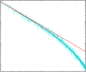
  $\omega ^{-2}$ power law. For real sawtooth waves, turbulent motions result in a diffusion-like process at wave fronts. The resulting rounding off of the fronts controls the high-frequency behaviour of the surface elevation spectrum. This is illustrated in figure 2, where two frequency subranges can be identified: an inertial subrange where the energy spectrum follows an $\omega ^{-2}$ tendency, and a second subrange where $E(\omega )$ decreases more rapidly with $\omega$. The latter range will be referred to as the diffusive subrange.

Figure 1. Example of a random sawtooth wave elevation signal in the inner surf zone, where  $\zeta$ denotes the surface elevation. Laboratory data from van Noorloos (Reference van Noorloos2003), experiment vN03-C3 (see table 1), wave gauge no. 64.

Figure 2. Example of a random sawtooth wave elevation spectrum in the inner surf zone. Laboratory data from van Noorloos (Reference van Noorloos2003), experiment vN03-C3 (see table 1), wave gauge no. 64. The cyan line indicates the sawtooth wave regime; the grey line indicates the beginning of the surf zone; the dashed line shows the  $\omega ^{-2}$ power law.
In this paper, we analyse the spectral behaviour of random sawtooth waves in the inner surf zone. We show that the energy spectrum, made up of the inertial and diffusive subranges, follows a universal shape. Based on analogies between inner surf zone waves and Burgers turbulence (i.e. ‘Burgulence’), we derive a theoretical law for the energy spectrum, and assess its validity from laboratory data. Within this theoretical framework, we analyse the properties of the dissipation spectrum and propose ways to improve its parametrization in stochastic spectral wave models.
2. Physical background
As waves propagate shoreward in decreasing water depth, wave height and nonlinearities increase, leading to wave breaking. After the initiation of breaking (spilling or plunging), a rapid change occurs in the wave shape over a relatively short distance. Shoreward of this region, the wave field reorganizes itself into a succession of relatively stable bore-like waves. This region, referred to by Svendsen, Madsen & Hansen (Reference Svendsen, Madsen and Hansen1978) as the inner surf zone (ISZ), covers a significant part of the surf zone for beaches of regular shape and gentle slope. The ISZ is a self-similar region, where waves are locally depth controlled (Thornton & Guza Reference Thornton and Guza1982). Specifically, the ratio of wave height to water depth remains nearly constant. As ISZ waves propagate, they maintain almost the same shape, consisting of a turbulent wave front and a quasi-linear back slope (e.g. Svendsen & Putrevu Reference Svendsen and Putrevu1996).
Due to the quasi-linear back slope, the non-hydrostatic effects are very small except at wave fronts (Martins et al. Reference Martins, Bonneton, Mouragues and Castelle2020). It has been shown that ISZ waves are nearly frequency non-dispersive (e.g. Thornton & Guza (Reference Thornton and Guza1982), and Martins et al. (Reference Martins, Bonneton and Michallet2021) and their figures 4g,h). This explains the presence of sawtooth waves (see figure 1), which are a characteristic feature of nonlinear non-dispersive wave phenomena, such as nonlinear acoustic waves (Gurbatov, Rudenko & Saichev Reference Gurbatov, Rudenko and Saichev2012). A sawtooth wave (SW) is a coherent structure that results from the competition between dissipation and nonlinearities. Another well-known coherent wave structure, occurring in nonlinear weakly dispersive regimes, is the solitary wave, which results from the balance between dispersion and nonlinearities. However, stable solitary waves occur only in idealized situations, whereas quasi-stable SWs occur in complex natural environments such as the ISZ.
Our study aims to comprehend the spectral behaviour of random SW fields in the ISZ. Our approach is based on the fact that basic characteristics of energy and dissipation spectra within the inertial frequency subrange can be inferred from the SW geometry. For instance, deriving the  $\omega ^{-2}$ power law for the energy spectrum, from a periodic SW signal with discontinuities at wave fronts, is a straightforward process. Furthermore, Kirby & Kaihatu (Reference Kirby and Kaihatu1997) showed an equipartition of the dissipation over the spectrum (i.e. ‘white spectrum’) within the inertial subrange. These authors proposed that this phenomenon arises from the fact that dissipation manifests in the space–time domain as a sequence of isolated spike-like processes. To gain a deeper understanding of ISZ energy and dissipation spectra, particularly in the diffusive frequency subrange, we will use the nonlinear shallow-water model, the simplest possible, capable of reproducing the SW shape and localized dissipation at wave fronts. The mathematical simplicity of the model is crucial in order to be able to derive analytical spectral laws.
Bonneton (Reference Bonneton2007) derived a one-way nonlinear shallow-water model, wherein wave fronts are represented by discontinuities (i.e. shocks) that describe correctly the dynamics of ISZ waves on gently sloping beaches. This model enables a good description of both the nonlinear wave distortion and the energy dissipation. We simplify the model by neglecting bottom variations, resulting in the equation
 \begin{equation} \frac{\partial \zeta}{\partial t}+c_0\,\frac{\partial \zeta}{\partial x}+\frac{3}{2}\,c_0\,\frac{\zeta}{h_0}\,\frac{\partial \zeta}{\partial x}=0 , \end{equation}
where  $\zeta$ is the surface elevation, $h_0$ is the mean water depth, $c_0=\sqrt {gh_0}$, and $g$ is the acceleration due to gravity. Even though shoaling effects are not considered, wave solutions provided by (2.1) bear a strong resemblance to waves in the ISZ, characterized by their sawtooth shape and localized energy dissipation at wave fronts. However, in essence, this shock-wave approach cannot describe the wave front structure, thus the energy spectrum in the diffusive subrange. In order to overcome this limitation, turbulent processes can be parametrized by including a diffusivity term $\nu _t({\partial ^2 \zeta }/{\partial x^2})$ on the right-hand side of (2.1), with $\nu _t$ a turbulent diffusion coefficient.
In the frame of reference moving at velocity  $c_0$, and making the change of variable
 \begin{equation} v=\frac{3c_0}{2 h_0}\,\zeta , \end{equation}
(2.1) can be rewritten as
 \begin{equation} \frac{\partial v}{\partial t}+v\,\frac{\partial v}{\partial x}=\nu_t\,\frac{\partial^2 v}{\partial x^2} . \end{equation}
Throughout this paper, we will use this idealized one-way nonlinear shallow-water model as a toy model to infer the SW spectral behaviour.
3. Burgers turbulence
3.1. Burgers model
To further simplify our wave problem, we consider in § 3 that the diffusion coefficient  $\nu _t$ is constant ( $\nu _t=\nu$). Equation (2.3) is then the well-known Burgers equation. It was introduced originally as a simple one-dimensional model to contribute to the study of turbulence (Burgers Reference Burgers1948). A synthesis on Burgers turbulence, also known as Burgulence, is presented in Frisch & Bec (Reference Frisch and Bec2002).
In this subsection, we consider freely decaying random waves  $v(x,t)$ that are statistically homogeneous in space, with zero mean. The equation for the mean energy $\boldsymbol {E}_v=\langle v^2 \rangle$ is
 \begin{equation} \frac{\partial \boldsymbol{E}_v}{\partial t}={-}\boldsymbol{D}_v , \end{equation}
where  $\boldsymbol {D}_v=2\nu \,\langle ({\partial v}/{\partial x})^2\rangle$ is the energy dissipation, and $\langle \,{\cdot}\, \rangle$ is the spatial mean.
A striking feature of Burgers solutions is the formation of shocks. Due to the nonlinear term, negative  $v$ slopes are steepened in time until they build up into diffusive shocks, where nonlinear and diffusive effects are balanced. For initial random conditions, the wave field tends towards an irregular sawtooth profile, quite similar to that of SWs in the ISZ (figure 1).
Two main characteristic scales are involved in the SW regime:  $\lambda _m$ is the mean distance between adjacent wave fronts, and $V_c$ is the characteristic scale of velocity jumps at wave fronts. The wave field is then controlled by two length scales: a macroscopic one, $\lambda _m$, and a small one, the average shock thickness $\delta \sim {\nu }/{V_c}$. Consequently, the problem is governed by one dimensionless parameter, the Burgers-type Reynolds number $R_B={V_c \lambda _m}/{\nu }$. It is well established that for wavenumbers ranging from $k_m=2{\rm \pi} /\lambda _m$ to the diffusive wavenumber $k_\nu$ ( $k_\nu \sim \delta ^{-1}$), the Burgers energy spectrum follows a $k^{-2}$ power law (e.g. Tatsumi Reference Tatsumi1969). This $k^{-2}$ subrange is followed at high $k$ by a diffusive subrange where the energy decreases more rapidly.
We will see later that ISZ waves are characterized by moderate Reynolds numbers of approximately a few hundreds ( $R_B \sim 100\unicode{x2013}500$). In this section, we analyse the spectral characteristics of Burgers waves for this $R_B$ range. It should be noted that most studies on Burgulence, unlike ours, focus on regimes with very high $R_B$. When referring to an ISZ wave, $R_B$ must be distinguished from the classical Reynolds number based on the kinematic viscosity. Before analysing random waves, we start by studying the nonlinear dynamics of periodic SWs. This idealized case is very useful, first for understanding basic nonlinear and dissipative processes in the spectral space, and second by serving as a basis for the development of a random SW theory.
3.2. Periodic sawtooth waves
In the non-diffusive case ( $\nu =0$), the derivation of the periodic SW Burgers solution, $v_{i}(x,t)$, from the method of characteristics is straightforward and gives
 \begin{equation} v_{i}=\frac{V_J(t)}{2}\left(\frac{2x}{\lambda} -\text{sgn}(x) \right), \quad x \in\left[-\frac{\lambda}{2},\frac{\lambda}{2}\right], \end{equation}
where  $\lambda$ is the wavelength, $V_J(t)={V_0}/({1+V_0t/\lambda })$ is the velocity jump across the inviscid shock (located in $x=0$), and $V_0$ is the velocity jump at $t=0$. Khokhlov derived an exact SW solution of the diffusive Burgers equation (see Gurbatov et al. (Reference Gurbatov, Rudenko and Saichev2012)):
 \begin{equation} v=\frac{V_J(t)}{2}\left(\frac{2x}{\lambda} -\tanh{\frac{V_J(t)\,x}{4\nu}} \right) . \end{equation}
This solution is not periodic, but for large Reynolds numbers it becomes quasi-periodic between  $x=-\lambda /2$ and $x=\lambda /2$, with a diffusive front located in $x=0$. The dimensionless velocity jump $\delta v_b=\left (v({\lambda }/{2}^-)-v({\lambda }/{2}^+)\right )/V_J=1-\tanh ({{R_B}/{8}})$ is an exponentially decreasing function of $R_B$. For the $R_B$ values that concern us, we can consider the solution (3.3) as periodic due to the small value of $\delta v_b$ ( $\delta v_b < 10^{-11}$).
For large  $R_B$, an approximate relationship of total dissipation $\boldsymbol {D}_v$ can be derived. Using (3.3) and retaining only the leading terms in an expansion in powers of $R_B$ gives
 \begin{equation} \left\langle\left(\frac{\partial v }{\partial x}\right)^2\right\rangle=\frac{1}{12}\,\frac{V_J^3 }{\nu \lambda} \end{equation}
and then
 \begin{equation} \boldsymbol{D}_v=\frac{1}{6}\,\frac{V_J^3}{\lambda} . \end{equation}
This shows that for  $R_B$ of interest, the total dissipation is virtually independent of $\nu$.
One of the main objectives of this paper is to analyse the spectral behaviour of SWs. In the case of periodic waves, it is possible to derive an expression for the energy spectral density from the Khokhlov solution (3.3) (see § A.1 in the supplementary material available at https://doi.org/10.1017/jfm.2023.878). This expression is written as
 \begin{equation} {\mathcal{E}}_{v_n}=2\nu^2 k_p^2\,\text{csch}^2\left( \frac{k_n}{k_\nu} \right), \end{equation}
where  ${\mathcal {E}}_{v_n}={v_n^2}/{2}$ is the energy spectral density, $v_n$ is the $n$th Fourier coefficient of $v$,
$v$,  $k_p={2{\rm \pi} }/{\lambda }$, $k_n=n k_p$ and $k_\nu ={V_J}/{2{\rm \pi} \nu }$. For $k_n/k_\nu \ll 1$, ${\mathcal {E}}_{v_n}$ follows a $k_n^{-2}$ power law:
 \begin{equation} {\mathcal{E}}_{v_n}=\frac{2V_J^2 }{\lambda^2}\,k_n^{{-}2}. \end{equation}
This last relation is also the exact energy spectral density of the non-diffusive SW solution (3.2). For  $k_n/k_\nu \gg 1$, ${\mathcal {E}}_{v_n}$ decreases exponentially with $k_n$. In the following, the inertial and diffusive subranges will be defined respectively as $k\in [k_p,k_\nu ]$ and $k\in [k_\nu,\infty ]$. The dimensionless width of the inertial subrange, $(k_\nu -k_p)/k_p$, increases linearly with $R_B$, since $k_\nu /k_p=R_B/(4{\rm \pi} ^2)$.
Substituting the Fourier series representation of  $v$ into the Burgers equation, we obtain the spectral energy equation
 \begin{equation} \frac{{\rm d}}{{\rm d}\,t}{\mathcal{E}}_{v_n}+{\mathcal{T}}_{v_n}={-}{\mathcal{D}}_{v_n} , \end{equation}
where  ${\mathcal {D}}_{v_n}=2\nu k_n^2 {\mathcal {E}}_{v_n}$ is the dissipation spectrum, and ${\mathcal {T}}_{v_n}$ the nonlinear transfer function. This last can be expressed as
 \begin{equation} {\mathcal{T}}_{v_n}=\frac{k_n}{4}\,v_n \sum_{m=1}^{n-1} v_m v_{n-m}-\frac{k_n}{2}\,v_n\sum_{m=1}^\infty v_m v_{n+m} , \end{equation}
where the first term on the right-hand side represents the triad sum interactions of components  $(m,n-m)$, and the second term represents the triad difference interactions of components $(m,n+m)$.
In order to better understand the spectral behaviour of dissipation and nonlinear interactions, we analyse the different terms in (3.8). Substituting (3.6) into  ${\mathcal {D}}_{v_n}=2\nu k_n^2 {\mathcal {E}}_{v_n}$, we get the dissipation spectrum
 \begin{equation} {\mathcal{D}}_{v_n}=4\nu^3 k_p^2 k_n^2\,\text{csch}^2\left( \frac{k_n}{k_\nu} \right) , \end{equation}
which is a decreasing function of  $k_n$. For $k_n/k_\nu \ll 1$, the dissipation spectrum given by
 \begin{equation} {\mathcal{D}}_{v_n}=\frac{4\nu V_J^2 }{\lambda^2} \end{equation}
is constant. The nonlinear transfer function can be obtained from  ${\mathcal {T}}_{v_n}=-(({{\rm d}}{\mathcal {E}}_{v_n}/{{\rm d}\,t}) + {\mathcal {D}}_{v_n})$, which results in
 \begin{equation} {\mathcal{T}}_{v_n}={-}2\nu k_n \left(k_n-k_p \coth \left( \frac{k_n}{k_\nu} \right) \right) {\mathcal{E}}_{v_n} . \end{equation}
 Figure 3 illustrates the contribution of each term in the spectral energy equation (3.8). We consider two SW fields with the same  $V_J$ and $\lambda$ but two contrasting Reynolds numbers $R_B=100$ and $R_B=500$ (respectively, minimum and maximum $R_B$ values observed in the ISZ experiments discussed in § 5). This means that we analyse two similar wave fields that have almost the same shape except at the wave front. Figure 3 shows that the temporal rate of change of the energy spectrum, ${{\rm d}}{\mathcal {E}}_{v_n}/{{\rm d}\,t}$, is virtually independent of $R_B$. This temporal rate of change follows the approximate relation for large $R_B$
$R_B$
 \begin{equation} \frac{{\rm d}}{{\rm d}\,t}{\mathcal{E}}_{v_n}={-}\frac{\boldsymbol{D}_v}{\boldsymbol{E}_v}\,{\mathcal{E}}_{v_n} , \end{equation}
where  $\boldsymbol {E}_v={V_J^2}/{12}$, and $\boldsymbol {D}_v$ and ${\mathcal {E}}_{v_n}$ are given by (3.5) and (3.7), respectively. This explains why the energy spectrum shape is practically preserved as SWs evolve with time. Contrary to ${{\rm d}}{\mathcal {E}}_{v_n}/{{\rm d}\,t}$, the dissipation spectrum ${\mathcal {D}}_{v_n}$ and the nonlinear transfer function ${\mathcal {T}}_{v_n}$ are strongly dependent on $R_B$. For the highest $R_B$ ( $R_B=500$), figure 3 shows that ${\mathcal {T}}_{v_1} \gg {\mathcal {D}}_{v_1}$, meaning that for the first wave mode (the most energetic), the rate of change of the energy spectrum is controlled mainly by energy transfer to higher wavenumbers. By contrast, for the lower $R_B$ ( $R_B=100$), ${\mathcal {T}}_{v_1}$ is of the same order of magnitude as ${\mathcal {D}}_{v_1}$, thus the nonlinear energy transfer and the energy dissipation contribute nearly equally to the energy decrease with time. We can see in figure 3 that ${\mathcal {D}}_{v_n}$ is nearly constant in the inertial subrange following (3.11), and decreases strongly in the high wavenumber tail of the spectrum (i.e. the diffusive subrange). In the diffusive subrange, $\lvert {{\rm d}}{\mathcal {E}}_{v_n}/{{\rm d}\,t} \rvert$ is much smaller than ${\mathcal {D}}_{v_n}$ and $\lvert {\mathcal {T}}_{v_n}\lvert$. This means that for high wavenumbers, there is a balance between the dissipation and the nonlinear energy transfer from low wavenumbers. This result seems in line with surf zone field observations by Herbers, Russnogle & Elgar (Reference Herbers, Russnogle and Elgar2000).

Figure 3. Dissipation spectrum and nonlinear transfer function for two SW solutions with the same  $V_J$ and $\lambda$ but distinct Reynolds numbers: $R_B=100$ (continuous lines) and $R_B=500$ (dash-dotted lines). Red lines indicate ${\mathcal {D}}_{v_n}$ (3.10); black lines indicate ${\mathcal {T}}_{v_n}$ (3.12); blue lines indicate ${{\rm d}}{\mathcal {E}}_{v_n}/{{\rm d}\,t} =-({\mathcal {D}}_{v_n}+ {\mathcal {T}}_{v_n} )$; dotted lines indicate positions of $k_\nu /k_p$. For the sake of clarity, we use lines (continuous or dash-dotted) to represent the discrete spectra.
To summarize this part,  ${{\rm d}}{\mathcal {E}}_{v_n}/{{\rm d}\,t}$ is governed primarily not by nonlinear interactions, even at low $k_n$, but rather by the competition between ${\mathcal {D}}_{v_n}$ and ${\mathcal {T}}_{v_n}$, which are both strongly dependent on diffusion processes at wave fronts. This conclusion, obtained for periodic SW, cannot be applied directly to ISZ random SW, which are a more complex phenomenon. However, these results may give ideas on how diffusive processes could affect the dissipation and the nonlinear interactions of ISZ SWs.
3.3. Random sawtooth waves
We now consider freely decaying random solutions  $v(x,t)$ that are statistically homogeneous in space with zero mean. The power spectral density $\varPhi (k,t)$ is the Fourier transform of the autocorrelation function $R(r)$:
 \begin{equation} \varPhi(k,t)=\frac{1}{2{\rm \pi}} \int_{-\infty}^\infty R(r) \exp(-{\rm i}kr)\,{\rm d}r , \end{equation}
where  $R(r,t)=\langle v(x,t)\,v(x+r,t)\rangle$. As $\varPhi (k,t)$ is an even function of $k$, we limit our analysis to $k \geq 0$, and denote $E_v(k,t)=2 \varPhi (k,t)$ the power spectral density function. With this notation, the total energy $\boldsymbol {E}_v=\langle v^2\rangle =\int _{-\infty }^\infty \varPhi (k)\, {\rm d}k$ can be expressed as
 \begin{equation} \boldsymbol{E}_v=\int_0^\infty E_v(k) \,{\rm d}k . \end{equation}
Throughout the paper,  $E_v$ will denote the energy spectrum. In the spectral space, the energy equation is given by
 \begin{equation} \frac{\partial E_v }{\partial t}+T_v={-}D_v , \end{equation}
where  $D_v(k,t)=2\nu k^2\,E_v(k,t)$ is the spectral energy dissipation, $T_v(k,t)=-k\int _{-\infty }^\infty \mathrm{Im} (B)\,{\rm d}l$ is the nonlinear transfer term, and $B(k,l,t)$ is the bispectrum.
Saffman (Reference Saffman1968) assumed that the periodic solution (3.3) reproduces the qualitative features of the small-scale behaviour of random SWs. From this hypothesis, he derived an expression for the energy spectrum, which is consistent with (3.6) obtained for the energy density function of periodic SWs. The equation for the energy spectrum is given by
 \begin{equation} E_v(k,t)=2\nu^2\,k_m(t)\,\text{csch}^2 \left(\frac{k}{k_\nu(t)} \right), \quad k\in[k_m,\infty] , \end{equation}
where  $k_\nu ={V_c}/{2 {\rm \pi}\nu }$ is the diffusive wavenumber, $V_c$ is the characteristic scale of $v$-jumps at wave fronts, $k_m=2{\rm \pi} /\lambda _m$, and $\lambda _m$ is the mean distance between adjacent wave fronts. The Reynolds number $R_B={V_c\lambda _m}/{\nu }$ can be expressed as $R_B=4{\rm \pi} ^2({k_\nu }/{k_m})$. The derivation of Saffman (Reference Saffman1968) equation is presented in § A.2 of the supplementary material, where we have both clarified the definition of the characteristic horizontal length scale and corrected an error in the hyperbolic cosecant term. This theory applies to short waves (i.e. SW scale) and not to wavenumbers smaller than approximately $k_m$. For the sake of clarity, explicit reference to time has been omitted in the following equations.
For periodic SWs, the definition of the characteristic scale of  $v$-jumps, $V_J$, is straightforward. It is the non-diffusive $v$-jump associated with the diffusive SW solution (3.3). The characteristic $v$-scale, $V_c$, in random SW fields is not explicit. It can be obtained implicitly from $\tilde {\boldsymbol {E}}_v=\int _{k_m}^\infty E_v(k) \,{\rm d}k$, the total energy over the wavenumber range $[k_m,\infty ]$. By integrating (3.17) from $k_m$ to $\infty$, we obtain
 \begin{equation} \tilde{\boldsymbol{E}}_v=2\nu^2 k_m k_\nu \left(\coth(k_m/k_\nu)-1\right) . \end{equation}
Given  $k_m$ and $\tilde {\boldsymbol {E}}_v=\int _{k_m}^\infty E_v(k) \,{\rm d}k$, the implicit equation (3.18) yields $k_\nu$ and then $V_c$. Thus, for a given random SW field characterized by $k_m$ and $\tilde {\boldsymbol {E}}_v$, (3.17) can predict the energy spectrum.
For  $k \ll k_\nu$, $E_v(k)$ follows a $k^{-2}$ power law independent of the diffusion coefficient $\nu$,
 \begin{equation} E_v(k)=\left(\frac{k_m V_c^2}{2{\rm \pi}^2} \right)k^{{-}2} , \end{equation}
and for  $k \gg k_\nu$, $E(k)$ decreases exponentially with $k$,
$k$,
 \begin{equation} E_v(k)=8\nu^2 k_m \exp \left({-}2\,\frac{k}{k_\nu} \right) . \end{equation}
The dissipation spectrum  $D_v(k,t)=2\nu k^2\,E_v(k,t)$ is given by
 \begin{equation} D_v(k)=4\nu^3 k_m k^2\,\text{csch}^2 \left(\frac{k}{k_\nu} \right), \quad k\in[k_m,\infty] , \end{equation}
and its asymptotic form for small  $k$ is
 \begin{equation} D_v(k)=\frac{\nu k_m V_c^2}{{\rm \pi}^2} . \end{equation}
It is worth noting that at large scale, the dissipation spectrum is constant, which means that there is equipartition of dissipation over the spectrum. The exponential decay of  $E_v(k)$ at large wavenumbers guarantees that the $k$-integrated dissipation, $\tilde {\boldsymbol {D}}_v=\int _{k_m}^\infty D_v(k) \,{\rm d}k$, is finite. To my knowledge, the theoretical model (3.17) has never been validated. In order to test the validity of this model, we have computed numerically random SW solutions of the Burgers equation. It is solved with a spectral method where aliasing is avoided by using the so-called $3/2$ rule. The initial random $v$-field, $v_0(x)=v(x,0)$, is specified in the Fourier space by the energy spectrum
 \begin{equation} E_0(k)=E_0\,\frac{k}{k_p}\exp\left(-\frac{1}{2}\,((k/k_p)^2-1 )\right) , \end{equation}
where  $k_p=2{\rm \pi} /\lambda _p$ is the peak wavenumber, and $E_0$ is the energy at $k_p$. The phase of each wavenumber is assigned a random value in the range $[0,2{\rm \pi} ]$. The length of the domain covers $2^8 \lambda _p$ and is discretized over $2^{16}$ grid points. The computed spectra $E_v(k,t)$ are estimated by an ensemble average over 1000 realizations.
Figure 4 illustrates the time evolution of the energy spectrum. The cascade of energy towards high wavenumbers, due to nonlinear triad interactions, leads to a rapid transition to an established SW regime. In this regime, the theoretical law (3.17) gives a very good description of the numerically computed spectra. The inertial and diffusive subranges are well represented by the  $k^{-2}$ power law (3.19) and by an exponential decrease (3.20), respectively. However, (3.17) tends to slightly underestimate the numerically computed spectrum at large wavenumbers ( $k>20 k_p$), whatever the numerical resolution. Contrary to the monochromatic case, the wavenumber $k_m$ is not constant and decreases with time due to shock merging. Consequently, the inertial subrange width, and thus the Reynolds number, decreases at a slower rate than in the monochromatic case. The time evolution of the dissipation spectrum is shown in figure 5. We observe very good agreement between the theoretical law (3.21) and the numerically computed dissipation spectra. In the inertial subrange, the dissipation is constant, in agreement with the non-diffusive SW theory (3.22). Then, in the diffusive subrange, the dissipation decreases exponentially. It is worth noting that for Burgers turbulence, the dissipation occurs mainly in the inertial subrange, unlike the classical hydrodynamic turbulence where dissipation occurs at smaller scale.

Figure 4. Time evolution of the power spectral density for an initial condition given by (3.23). Dashed line indicates initial condition; cyan lines indicate numerical simulations at dimensionless times  $t/t_*=1.45, 2.90, 4.85$ (corresponding to Reynolds numbers $R_B=443, 380, 363$), where $t_*=1/(k_p \sqrt {E_{T_0}})$; black line indicates theoretical model (3.17) starting from $k=k_m$; red line indicates $k^{-2}$ power law (3.19); red plus symbol indicates position of $k_\nu /k_p$. The length of the domain covers $2^8 \lambda _p$ and is discretized over $2^{16}$ grid points. Spectra have been averaged over 1000 realizations.

Figure 5. Time evolution of the dissipation spectrum for an initial condition given by (3.23). Cyan lines indicate numerical simulations at dimensionless times  $t/t_*=1.45, 2.90, 4.85$ (corresponding to Reynolds numbers $R_B=443, 380, 363$), where $t_*={1}/{k_p \sqrt {E_{T_0}}}$; black lines indicate the theoretical model (3.21) starting from $k=k_m$; red lines indicate (3.22). The length of the domain covers $2^8 \lambda _p$ and is discretized over $2^{16}$ grid points. Spectra have been averaged over 1000 realizations.
4. Analytical energy spectrum for ISZ waves
The above results for the Burgers equation apply directly to the one-way shallow-water equation (2.1). Therefore, we can describe the spectral behaviour of irregular SWs, statistically homogeneous in space, propagating freely in a constant water depth at celerity  $c_0=\sqrt {gh_0}$. However, ISZ waves are not statistically homogeneous in space, since they are forced at the offshore limit of the ISZ and propagate over a varying mean water depth $h_0(x)$. Subsequently, we will make the strong assumption that for slowly varying bathymetry, the shape of the energy spectrum in the wavenumber space can be estimated using the corrected Saffman equation (3.17). It should also be noted that unlike Burgers-like waves, ISZ waves are asymmetric with respect to the mean water level (i.e. are skewed). In fact, their back slope is not linear but convex. However, the curvature is small enough not to affect the $k^{-2}$ tendency of the energy spectrum in the inertial subrange.
Laboratory and field experiments (Thornton & Guza Reference Thornton and Guza1982; Elgar & Guza Reference Elgar and Guza1985a; Martins et al. Reference Martins, Bonneton and Michallet2021) showed that in the ISZ, most wave components of the spectrum are bounded and propagate to the same celerity  $c_m$ close to the non-dispersive celerity in shallow water, $c_0$. From laboratory experiments analysed in § 5, we have verified that this spectral behaviour also holds for high frequencies in the diffusive subrange. The ISZ celerity can be estimated by the relation $c_m=\alpha _c c_0$, where $\alpha _c \simeq 1.1\unicode{x2013}1.2$ (Tissier et al. Reference Tissier, Bonneton, Almar, Castelle, Bonneton and Nahon2011; Martins et al. Reference Martins, Bonneton and Michallet2021). Using the dispersion relation $\omega =c_m k$, we can estimate the energy spectrum in the frequency domain, $E_v(\omega )$, from that in the wavenumber domain. The spectrum $E_v(\omega )$ can then be written
 \begin{equation} E_v(\omega)=\frac{2\nu_c^2 \omega_m}{c_0^2}\,\text{csch}^2 \left(\frac{\omega}{\omega_\nu} \right), \quad\omega \in[\omega_m,\infty] , \end{equation}
where  $\nu _c(x)$ is a characteristic turbulent diffusion coefficient that varies in space, and $\omega _m=2{\rm \pi} /T_m$, with $T_m$ the mean time between adjacent wave fronts, and $\omega _\nu$ the diffusive angular frequency. For the sake of simplicity, the empirical coefficient $\alpha _c$, which is close to 1, does not appear in the spectrum equation. It has been integrated into the diffusion coefficient, resulting in the actual diffusion coefficient being equal to $\alpha _c \nu _c$.
Making the change of variable (2.2) to come back to the physical scale  $\zeta$, we obtain the following expression for the energy spectrum in the frequency domain $E(\omega )$:
 \begin{equation} E(\omega)=\frac{8}{9}\,\frac{\nu_c^2}{g}\,\omega_m\,\text{csch}^2\left( \frac{\omega}{\omega_\nu} \right), \quad \omega\in[\omega_m,\infty] , \end{equation}
where  $\omega _\nu =({3}/{4{\rm \pi} })({gH_c}/{\nu _c})$, and $H_c$ is the characteristic scale of elevation jumps at wave fronts. This scale is related to the characteristic scale of $v$-jumps $V_c$ by $H_c=\tfrac {2}{3}({h_0}/{c_0}) V_c$. Contrary to the Burgers case, the turbulent diffusion coefficient $\nu _c$ is here an unknown of the problem. The total wave energy is defined by $\boldsymbol {E}=\overline {g \zeta ^2} =\int _0^\infty E(\omega ) \,{\rm d}\omega$, where $\overline {(\,{\cdot}\,)}$ is the time average operator. For $\omega \ll \omega _\nu$, $E(\omega )$ follows an $\omega ^{-2}$ power law,
 \begin{equation} E(\omega)=\left(\frac{g\omega_m H_c^2}{2{\rm \pi}^2} \right)\omega^{{-}2} , \end{equation}
and for  $\omega \gg \omega _\nu$, it decreases exponentially with $\omega$,
 \begin{equation} E(\omega)=\frac{32}{9}\,\frac{\nu_c^2}{g}\,\omega_m \exp \left({-}2\,\frac{\omega}{\omega_\nu} \right). \end{equation}
The energy spectrum can be expressed in a dimensionless form as
 \begin{equation} \frac{E(\omega)}{E_m}=\left( \frac{\omega_m}{\omega_\nu}\right) ^2 \text{csch}^2\left(\frac{\omega_m}{\omega_\nu}\,\frac{\omega}{\omega_m} \right) , \end{equation}
where  $E_m={g H_c^2}/{2{\rm \pi} ^2\omega _m}$. The shape of the energy spectrum is thus controlled entirely by the dimensionless number $\omega _m/\omega _\nu$, or equivalently by the Reynolds number $R_B=4{\rm \pi} ^2({\omega _\nu }/{\omega _m})=\tfrac {3}{2}({gH_c T_m}/{\nu _c})$. In the following, the inertial and diffusive subranges will be defined respectively as $\omega \in [\omega _m,\omega _\nu ]$ and $\omega \in [\omega _\nu,\infty ]$. The dimensionless width of the inertial subrange, $(\omega _\nu -\omega _m)/\omega _m$, increases linearly with $R_B$.
The nonlinearities of shallow-water waves are usually characterized by the dimensionless parameter  $\epsilon ={H_c/2}/{h_0}$, which quantifies the relative importance of nonlinearities over the linear advection. For waves propagating in the ISZ over a regular low slope bottom, the nonlinearity parameter $\epsilon$ changes very little and has a value of approximately 0.2–0.3 (e.g. Svendsen et al. Reference Svendsen, Madsen and Hansen1978; Thornton & Guza Reference Thornton and Guza1982). Reynolds number $R_B$, on the other hand, quantifies the relative importance of nonlinearities with respect to turbulent diffusion. We will see in the next section that this second nonlinearity parameter, contrary to $\epsilon$, evolves strongly as waves propagate in the ISZ.
5. Application to laboratory experiments
5.1. Description of datasets
The theoretical approach developed above is now evaluated against laboratory experiments on random wave propagation and breaking on a uniform slope. Six laboratory datasets are used: one from Mase & Kirby (Reference Mase and Kirby1993) (hereafter MK93), three from Bowen & Kirby (Reference Bowen and Kirby1994) (BK94), and two from van Noorloos (Reference van Noorloos2003) (vN03). These experiments cover a large variety of incident random wave conditions in terms of frequency peak  $f_p$, wave height $H_{i}$, and spectral shape. The random waves were generated at the wave paddle using random realizations of analytical single-peaked spectra. Mase & Kirby (Reference Mase and Kirby1993) chose a Pierson–Moskowitz spectrum that can be seen in figure 6(c) (blue line). van Noorloos (Reference van Noorloos2003) used a JONSWAP spectrum with a peak-enhancement factor $\gamma =3.3$, which provides a much sharper frequency peak than that of the Pierson–Moskowitz spectrum (see blue lines in figures 6a,b). Bowen & Kirby (Reference Bowen and Kirby1994) chose a TMA spectrum, which is an extension of the JONSWAP spectrum describing waves in finite depth. In shallow water, the TMA spectrum follows an $\omega ^{-3}$ power law, which results in a broader spectrum than the JONSWAP spectrum (see blue lines in figures 6d–f). In all these experiments, the wave gauges are sampled at frequency 25 Hz. For our spectral analysis, we will consider frequency lower than half the Nyquist frequency, i.e. $\omega < \omega _{max}=40$ rad s $^{-1}$. The smallest wavelength, associated with $\omega _{max}$, is approximately 10 cm, a scale much larger than capillary wave scales. The experimental parameters of the six datasets are given in table 1.

Figure 6. Energy spectra for (a) vN03-C3, (b) vN03-D3, (c) MK93, (d) BK94-7, (e) BK94-8, and ( f) BK94-9. Blue line indicates incident wave spectrum; grey line indicates spectrum at the breaking point; cyan line indicates ISZ spectrum in a mean water depth  $h_0= 5.5$ cm; black line indicates (4.2); red line indicates (4.3). Blue cross indicates position of $\omega _m$; red cross indicates position of $\omega _\nu$.
Table 1. Experimental parameters:  $H_i$, incident wave height; $h_i$, water depth; $f_p$, peak frequency; $\gamma$, peak-enhancement factor; $s$, bottom slope; $f_s$, sampling rate.

As incoming waves shoal, energy is transferred from the most energetic portion of the energy spectrum (around the spectral peak) to both higher and lower frequencies (figure 6). At the breaking point, the spectrum shape depends strongly on the incident wave spectrum. For instance, narrow-band spectra (see figures 6a,b) develop harmonic peaks of the fundamental frequency and infragravity waves (i.e. waves with frequency lower than approximately  $0.5f_p$) that are both significantly larger than those associated with broad-band incident wave spectra. By contrast, in the ISZ, the high-frequency part ( $\omega > \omega _m$) of the wave spectrum always has a regular shape with an $\omega ^{-2}$ tendency in the inertial subrange, whatever the incident wave conditions. The $\omega ^{-2}$ tendency of ISZ wave spectra was already noticed by Kirby & Kaihatu (Reference Kirby and Kaihatu1997). While the shape of the high-frequency part of the ISZ spectrum is almost independent of the incident wave conditions, this is not the case for the frequency bounds of the inertial subrange. The lower bound $\omega _m$ is an increasing function of the frequency peak of the incident wave spectrum $\omega _p$. Moreover, the time evolution of $\omega _m$ is controlled in the surf zone by the wave front merging phenomenon. Tissier, Bonneton & Ruessink (Reference Tissier, Bonneton and Ruessink2017) showed that this phenomenon is favoured by the presence of infragravity waves whose intensity depends on incident wave conditions.
5.2. Assessment of the analytical wave energy spectrum
To apply the theoretical spectrum (4.2) to a laboratory dataset, it is necessary to know the three parameters  $\omega _m$, $\omega _\nu$ and $\nu _c$. The parameter $\nu _c$ can be substituted by the energy $\tilde {\boldsymbol {E}}=\int _{\omega _m}^\infty E(\omega ) \,{\rm d}\omega$ using the equation
 \begin{equation} \tilde{\boldsymbol{E}}=\frac{8}{9}\,\frac{\nu_c^2}{g}\,\omega_m \omega_\nu \left(\coth(\omega_m/\omega_\nu)-1\right) . \end{equation}
For each dataset, the mean time  $T_m$ between adjacent wave fronts is obtained from a wave-by-wave analysis that identifies each SW front. The energy $\tilde {\boldsymbol {E}}$ is then calculated by integrating the experimental energy spectrum from $\omega _m=2{\rm \pi} /T_m$ to the Nyquist frequency. The diffusive frequency $\omega _\nu$ is an unknown of the problem. To evaluate this frequency, we use a nonlinear least squares method to fit the measured spectrum with the theoretical one, rewritten in the form
 \begin{equation} \frac{E(\omega)}{\tilde{\boldsymbol{E}}}=\frac{\text{csch}^2\left( \dfrac{\omega}{\omega_\nu} \right)}{\omega_\nu \left(\coth(\omega_m/\omega_\nu)-1\right)} . \end{equation}
For the whole dataset, the diffusive frequency  $\omega _\nu$ ranges from 14.5 to 25.8 rad s $^{-1}$ (i.e. $f_\nu =\omega _\nu /(2{\rm \pi} ) \in [2.3,4.1]$ Hz). Knowing $\omega _\nu$, we obtain finally $\nu _c$ from (5.1).
Figure 6 shows ISZ spectra measured in 5 cm water depth for the six contrasting datasets (see table 1). Whatever the random wave forcing, the ISZ spectral shape is well described by the theoretical spectrum (4.2). The  $\omega ^{-2}$ tendency is identifiable on all measured spectra. However, this tendency is, of course, less marked for a small inertial subrange, i.e. small $R_B$ (e.g. see figure 6b) than for large $R_B$ (see figure 6f).
We are now interested in the evolution of the ISZ wave spectrum as waves propagate shoreward in decreasing water depth. The measured wave spectra are very well described by (4.2) irrespective of the dataset and the water depth (see figures 7 and 8, and in the supplementary material, figures 3–6). As illustrated in figure 9, by scaling measured wave spectra by  $E_a={8\nu _c^2\omega _m}/{9g}$, data collapse on a single curve given by the dimensionless universal spectrum equation
 \begin{equation} \frac{E}{E_a}= \text{csch}^2\left( \frac{\omega}{\omega_\nu} \right) . \end{equation}
Spectra differ only in their dimensionless inertial range width  $(\omega _\nu -\omega _m)/\omega _\nu$. We focus our analysis on two contrasting datasets: BK94-9 (figure 7) and vN03-C3 (figure 8). In both cases, we observe a decrease in $\omega _m$ as waves propagate (i.e. $h_0$ decreases), which is due to the bore merging phenomenon. This decrease is much stronger for vN03-C3 (from 3.53 to 1.99 rad s $^{-1}$) because large-amplitude infragravity waves favour bore merging (Tissier et al. Reference Tissier, Bonneton and Ruessink2017). However, as for the Burgers case (see figure 4), the shape of the energy spectrum at the SW scales, $\omega >\omega _m$, is not affected by low-frequency waves. The diffusive frequency $\omega _\nu$, which marks the transition between the inertial and diffusive subranges, increases significantly for BK94-9 (from 18.7 to 24.1 rad s $^{-1}$) and slightly for vN03-C3 (from 14.9 to 16.1 rad s $^{-1}$). For both experiments, we observe an increase in the inertial subrange width as waves propagate, and thus an increase in the Reynolds number $R_B$. This evolution is observable for all datasets, as can be seen in figure 10. This figure also shows that the Reynolds number is controlled primarily by the peak period $T_p$ of the incident wave field and is an increasing function of $T_p$. The increase of $R_B$ in decreasing water depth means that the relative importance of nonlinearities with respect to turbulent diffusion increases as waves propagate and thus as broken wave height decreases. This differs from what we have observed above for Burgers turbulence, where $R_B$ is an increasing function in $H_c$. It means that in the ISZ, the characteristic wave height $H_c$ decreases less rapidly than $\nu _c$ as $h_0$ decreases. Assuming that the turbulent diffusion coefficient is controlled mainly by $H_c$, dimensional analysis leads to the following relationship between $\nu _c$ and $H_c$:
 \begin{equation} \nu_c= \alpha_\nu g^{1/2}H_c^{3/2} , \end{equation}
where  $\alpha _\nu$ is a dimensionless coefficient. Similar scalings are used commonly to estimated eddy viscosity in the surf zone (e.g. Svendsen, Schäffer & Hansen Reference Svendsen, Schäffer and Hansen1987). Figure 11 shows that the turbulent diffusion coefficient $\nu _c$ follows an $H_c^{3/2}$ power law in agreement with (5.4). However, the value of the coefficient $\alpha _\nu$ depends on incident wave conditions. The relation (5.4) implies that $R_B$ evolves approximately as $H_c^{-1/2}T_m$ and is indeed a decreasing function of $h_0$. It is worth noting that our approach applies only to the ISZ. Indeed, the increase in $\nu _c$ with $H_c$ should not be valid in the vicinity of the onset of wave breaking.

Figure 7. Energy spectra at different locations in the ISZ for the BK94-9 experiment: (a)  $x=24.50$ m, ${h_0=7.6}$ cm; (b) $x=24.72$ m, $h_0=6.8$ cm; (c) $x=24.97$ m, $h_0=6.2$ cm; (d) $x=25.22$ m, $h_0=5.5$ cm;(e) $x=25.50$ m, $h_0=4.9$ cm; and ( f) $x=25.76$ m, $h_0=4.0$ cm. Grey line indicates spectrum at the breaking point; cyan line indicates ISZ spectrum at water depth $h_0$; black line indicates (4.2); red line indicates (4.3). Blue dashed line indicates position of $\omega _m$; red dashed line indicates position of $\omega _\nu$.

Figure 8. Energy spectra at different locations in the ISZ for the vN03-C3 experiment: (a) gauge 60,  $h_0=8.4$ cm; (b) gauge 61, $h_0=7.6$ cm; (c) gauge 62, $h_0=6.8$ cm; (d) gauge 63, $h_0=6.1$ cm; (e) gauge 64, $h_0=5.3$ cm; ( f) gauge 65, $h_0=4.5$ cm; (g) gauge 66, $h_0=3.7$ cm; and (h) gauge 67, $h_0=3.0$ cm. Grey line indicates spectrum at the breaking point; cyan line indicates ISZ spectrum at water depth $h_0$; black line indicates (4.2); red line indicates (4.3). Blue dashed line indicates position of $\omega _m$; red dashed line indicates position of $\omega _\nu$.

Figure 9. Dimensionless energy spectra  $E/E_a$ ( $E_a={8\nu _c^2\omega _m}/{9g}$) at different locations in the ISZ for the vN03-C3 experiment. Grey lines indicate measurements from gauges 60–67 ( $h_0$ from 8.4 cm to 3 cm); black line indicates (5.3); red line indicates $\omega ^{-2}$ power law.

Figure 10. Evolution of the Reynolds number  $R_B$ as a function of water depth $h_0$.

Figure 11. Evolution of the diffusion coefficient as a function of  $g^{1/2}H_c^{3/2}$.
6. Energy dissipation
Breaking-wave energy dissipation is one of the most important processes in the nearshore. In particular, it controls the mean wave-induced circulation (Bühler & Jacobson Reference Bühler and Jacobson2001; Bonneton et al. Reference Bonneton, Bruneau, Castelle and Marche2010). However, wave dissipation in the surf zone remains poorly understood and is modelled heuristically in stochastic spectral wave models (Cavaleri et al. Reference Cavaleri2018). The commonly used method in spectral models is in two steps: first, total dissipation  $\boldsymbol {D}$ is estimated using a parametric random wave model (e.g. Battjes & Janssen Reference Battjes and Janssen1978; Thornton & Guza Reference Thornton and Guza1983) based on an analogy between broken waves and non-diffusive (i.e. $R_B=\infty$) hydraulic jumps; and second, $\boldsymbol {D}$ is redistributed over frequencies following $D(\omega )=\varGamma (\omega )\,E(\omega )$, where $\varGamma (\omega )$ is an ad hoc function satisfying the condition $\int _0^\infty \varGamma (\omega )\,E(\omega )\,{\rm d}\omega =\boldsymbol {D}$. In most stochastic spectral models (e.g. operational wave models SWAN and WWIII), $\varGamma$ is given by the parametrization proposed by Eldeberky & Battjes (Reference Eldeberky and Battjes1996)
 \begin{equation} \varGamma(\omega)=\frac{\boldsymbol{D}}{\boldsymbol{E}}, \end{equation}
where  ${\boldsymbol {E}}$ is the total energy.
This method assumes implicitly that  $D$ is independent of turbulent diffusion processes at wave fronts and thus independent of the Reynolds number $R_B$. Even if the dynamics of random SWs in the ISZ is more complex than that of periodic SWs, it is worth noting that for the latter, the dissipation spectrum is strongly dependent on $R_B$. In the periodic case, it is the sum of $D$ and the nonlinear transfer function $T$ that is nearly independent of $R_B$ and can be approximated by $T(\omega )+D(\omega )=\varGamma \,E(\omega )$, where $\varGamma ={\boldsymbol {D}}/{\boldsymbol {E}}$ (see (3.13)), in a form resembling the parametrization (6.1).
Parametrization (6.1) is also based on the assumption that  $\varGamma$ is independent of $\omega$. However, several studies have shown that $\varGamma$ is an increasing function of $\omega$ (Mase & Kirby Reference Mase and Kirby1993; Chen, Guza & Elgar Reference Chen, Guza and Elgar1997; Elgar et al. Reference Elgar, Guza, Raubenheimer, Herbers and Gallagher1997; Kirby & Kaihatu Reference Kirby and Kaihatu1997; Herbers et al. Reference Herbers, Russnogle and Elgar2000; Kaihatu et al. Reference Kaihatu, Veeramony, Edwards and Kirby2007; Smit et al. Reference Smit, Janssen, Holthuijsen and Smith2014). Mase & Kirby (Reference Mase and Kirby1993) and Elgar et al. (Reference Elgar, Guza, Raubenheimer, Herbers and Gallagher1997), based on laboratory and field observations, respectively, identified a frequency-squared tendency for $\varGamma$. Mase & Kirby (Reference Mase and Kirby1993) noticed that this $\omega ^2$ dependence appears similar to that of the viscous damping term of the Burgers equation. Kirby & Kaihatu (Reference Kirby and Kaihatu1997) and Smit et al. (Reference Smit, Janssen, Holthuijsen and Smith2014), by performing numerical simulations with a time-dependent Boussinesq model and a non-hydrostatic model, respectively, confirmed the $\omega ^2$ dependence for $\varGamma$ in the ISZ. In this context, $\varGamma$ can be written as
 \begin{equation} \varGamma(\omega)=\alpha_\varGamma \omega^2 , \end{equation}
where  $\alpha _\varGamma$ is given by
 \begin{equation} \alpha_\varGamma = \frac{\boldsymbol{D}}{\int_0^\infty \omega^2\,E(\omega) \,{\rm d}\omega} . \end{equation}
Based on laboratory and field data, Chen et al. (Reference Chen, Guza and Elgar1997) demonstrated that spectral Boussinesq model predictions of wave skewness and asymmetry are more accurate with the dissipation parametrization given by (6.2) than by frequency-independent parametrization (6.1).
However, neither parametrization takes into account turbulent diffusion processes at wave fronts. On the other hand, the Burgers-like theory presented in § 4 and validated in § 5 allows us to obtain a relation between  $D(\omega )$ and $E(\omega )$,
 \begin{equation} D(\omega)=\frac{2\nu_c}{g h_0}\,\omega^2\,E(\omega) , \end{equation}
which takes into account the turbulent diffusion through  $\nu _c$. The frequency-squared dependence of (6.4) is in agreement with observations described just above. We have shown in § 5.2 that the diffusion coefficient is controlled mainly by the characteristic wave height (see (5.4) and figure 11). However, an accurate parametrization of $\nu _c$ will require the analysis of a larger dataset, including field observations. Relation (6.4) does not require an ad hoc parametrization of the total dissipation as is the case for previous approaches (cf. (6.1) and (6.2)). On the contrary, $\boldsymbol {D}$ is given explicitly by integrating (6.4) over frequencies, i.e. $\boldsymbol {D}=({2\nu _c}/{g h_0})\int _0^\infty \omega ^2\,E(\omega ) \,{\rm d}\omega$. By substituting the energy spectrum equation (4.2) into the last integral, we can obtain an approximate relation for the total dissipation for large $R_B$:
 \begin{equation} \boldsymbol{D}= \frac{g}{4h_0T_m}\,H_c^3 . \end{equation}
If we replace the characteristic wave height  $H_c$ by the root-mean-square wave height $H_{rms}$, this expression is similar to the empirical expression based on an analogy between broken waves and non-diffusive hydraulic jumps (Battjes & Janssen Reference Battjes and Janssen1978). The approximate relation (6.5) is not useful in itself, but it is very interesting because it highlights a connection between our approach and the classical non-diffusive one (Battjes & Janssen Reference Battjes and Janssen1978). Equation (6.4) applies only to the ISZ, but it could serve as a theoretical basis for developing new parametrizations of the dissipation spectrum in stochastic spectral models for the entire surf zone.
By combining the energy spectrum law (4.2) and (6.4), we obtain a theoretical law for the dissipation spectrum:
 \begin{equation} D(\omega)=\frac{16}{9}\,\frac{\nu_c^3}{g^2 h_0}\,\omega_m \omega^2\,\text{csch}^2\left( \frac{\omega}{\omega_\nu} \right), \quad \omega\in[\omega_m,\infty]. \end{equation}
The asymptotic form of (6.6) for  $\omega \ll \omega _\nu$ is given by
 \begin{equation} D(\omega)=\frac{\nu_c \omega_m H_c^2}{{\rm \pi}^2 h_0} . \end{equation}
 We now analyse the main characteristics of  $D(\omega )$, but without direct experimental validation of theoretical dissipation spectra. A dissipation spectrum computed by applying (6.4) to a measured energy spectrum is presented in figure 12. This dissipation spectrum compares well with the theoretical one in (6.6). We can see that $D(\omega )$ is not proportional to $E(\omega )$ but is nearly constant in the inertial subrange $[\omega _m, \omega _\nu ]$, with a value in agreement with (6.7). In other words, there is an equipartition of energy dissipation over the inertial subrange. This result is in agreement with observations by Kirby & Kaihatu (Reference Kirby and Kaihatu1997) and Kaihatu et al. (Reference Kaihatu, Veeramony, Edwards and Kirby2007). Kirby & Kaihatu (Reference Kirby and Kaihatu1997) proposed that this phenomenon arises from the fact that dissipation manifests in the space–time domain as a sequence of isolated spike-like processes. Contrary to energy, dissipation $D(\omega )$ is large up to high frequencies of approximately $\omega _\nu$. For example, at large Reynolds numbers ( $R_B\sim 400$), the dissipation $D(\omega _\nu )$ is approximately 0.72 times the maximum dissipation $D(\omega _m)$, while the energy ratio $E(\omega _\nu )/E(\omega _m)$ is approximately $10^{-2}$. In our datasets, $\omega _\nu$ can reach values up to $17\omega _p$ (see figure 7f). This means that a proper modelling of dissipation needs to consider a frequency range much larger than the one that is sufficient to properly estimate total energy. This is an important result in the context of spectral wave model development.

Figure 12. Dissipation spectrum in the ISZ. Cyan line indicates dissipation computed from a measured energy spectrum (see figure 8g) and (6.4), vN03-C3 experiment, gauge 66; solid black line indicates theoretical dissipation law (6.6) for  $\omega \in [\omega _m, \infty ]$; black dashed line indicates theoretical law (6.6) for $\omega \in [0,\omega _m]$, outside of its range of applicability; black dotted line indicates (6.7); blue dotted line indicates position of $\omega _m$; red dotted line indicates position of $\omega _\nu$.
7. Conclusion
The spectral behaviour of random SWs propagating in the ISZ has been analysed. We show that the elevation spectrum exhibits a universal shape. A theoretical spectrum has been derived based on the similarities between SWs in the ISZ and Burgers SW solutions. Very good agreement between this theoretical model and laboratory experiments covering a large range of incident random wave conditions is shown. The energy spectrum shape is determined by three parameters:  ${\omega _m=2{\rm \pi} /T_m}$, the diffusive frequency $\omega _\nu$, and the turbulent diffusion coefficient $\nu _c$. It is thus controlled by one dimensionless number defined as $R_B=4{\rm \pi} ^2({\omega _\nu }/{\omega _m})$, or equivalently as ${R_B=\tfrac {3}{2}({gH_c T_m}/{\nu _c})}$, where $H_c$ is the characteristic wave height. This Reynolds number quantifies the relative importance of nonlinearities with respect to turbulent diffusion. In the inertial frequency subrange, defined as $\omega \in [\omega _m,\omega _\nu ]$, the energy spectrum follows an $\omega ^{-2}$ tendency. An exponential decay of $E$ with $\omega$ is observed in the high-frequency diffusive subrange $\omega \in [\omega _\nu, \infty ]$. We have shown that the turbulent diffusion coefficient is controlled mainly by the characteristic wave height, following (5.4). Consequently, the Reynolds number evolves approximately as $H_c^{-1/2}T_m$. The nonlinearities thus increase as waves propagate in decreasing water depth. This explains why the inertial subrange and its $\omega ^{-2}$ tendency are more marked at the end of the ISZ than at the beginning. It is worth noting that information on turbulent processes in the ISZ can be provided indirectly by applying our theoretical model to high-frequency wave elevation measurements.
In stochastic spectral wave models, it is crucial to have a good parametrization of the dissipation spectrum  $D(\omega )$. Within the framework of our theoretical approach, we have derived an explicit relation between $D$ and $E$ (see (6.4)), showing a frequency-squared dependence in agreement with previous laboratory and field studies. Contrary to usual dissipation parametrizations, our relation does not require an empirical estimation of total dissipation $\boldsymbol {D}$. We must keep in mind that our approach has been developed for the SW regime in the ISZ and not for the entire surf zone. However, our model (6.4) could nevertheless be useful for developing new parametrizations of the dissipation spectrum for the entire surf zone.
An equation has been derived for describing the universal shape of the dissipation spectrum in the ISZ. It highlights that  $D$ remains nearly constant within the inertial subrange, and decreases exponentially within the diffusive subrange. The equipartition of dissipation over the inertial subrange is in agreement with previous observations. Contrary to energy, dissipation $D(\omega )$ is large up to high frequencies of approximately $\omega _\nu$. Consequently, a proper modelling of the dissipation needs to consider a much larger frequency range than the one containing most of the energy. Therefore, to characterize the spectral behaviour of surf zone waves in the field, it is crucial to be able to quantify accurately the surface elevation spectrum at high frequencies, up to approximately 1–2 Hz. Developments on both nonlinear reconstruction of wave elevation from pressure measurements (Bonneton & Lannes Reference Bonneton and Lannes2017; Bonneton et al. Reference Bonneton, Lannes, Martins and Michallet2018; Martins et al. Reference Martins, Bonneton, Mouragues and Castelle2020) and lidar methods (Brodie et al. Reference Brodie, Raubenheimer, Elgar, Slocum and McNinch2015; Martins et al. Reference Martins, Blenkinsopp, Power, Bruder, Puleo and Bergsma2017) should help to achieve this goal.
Supplementary material
Supplementary material is available at https://doi.org/10.1017/jfm.2023.878.
Acknowledgements
The author would like to thank J. Kirby for allowing the use of his experimental data (Mase & Kirby Reference Mase and Kirby1993; Bowen & Kirby Reference Bowen and Kirby1994) and A. van Dongeren for kindly providing the (van Noorloos Reference van Noorloos2003) dataset. I am also grateful to K. Martins for his valuable comments. I would like also to thank J.-F. Bony for his assistance in deriving Burgers energy spectra. Additionally, I would like to thank the associate editor and the three reviewers for their comments and suggestions, which have contributed to improving this paper.
Declaration of interests
The author reports no conflict of interest.


 Open access