


1. Introduction
Flows encountered in nature are exposed to spatial modulations, e.g. roughness represents topography modulations, and temperature patterns represent thermal modulations. Both effects can be used for intentional flow actuation, which, if properly designed, can give the flow new, practically relevant features. It is known that specific grooves lead to a reduction of friction losses in laminar (Mohammadi & Floryan Reference Mohammadi and Floryan2013) and turbulent (Walsh Reference Walsh1983; Chen et al. Reference Chen, Floryan, Chew and Khoo2016) flows and lead to energy-efficient, low-Reynolds-number chaotic stirring (Gepner & Floryan Reference Gepner and Floryan2020). It is also known that heating patterns (Hossain, Floryan & Floryan Reference Hossain, Floryan and Floryan2012; Floryan & Floryan Reference Floryan and Floryan2015; Hossain & Floryan Reference Hossain and Floryan2015), as well as transpiration patterns (Jiao & Floryan Reference Jiao and Floryan2021a,Reference Jiao and Floryanb), reduce frictional losses in laminar flows. A combination of groove and heating patterns may significantly reduce or increase losses depending on the relative position of both patterns (Hossain & Floryan Reference Hossain and Floryan2020). Their proper combination may activate the pattern interaction effect (Floryan & Inasawa Reference Floryan and Inasawa2021), generating thermal drift (Abtahi & Floryan Reference Abtahi and Floryan2017; Inasawa, Hara & Floryan Reference Inasawa, Hara and Floryan2021). It is further known that selective vibration patterns reduce pressure losses while others increase such losses while increasing flow mixing (Floryan & Haq Reference Floryan and Haq2022; Haq & Floryan Reference Haq and Floryan2023).
The transition of spatially modulated flows to secondary states restricts the effectiveness of modulations when drag reduction is of interest. This transition may be desired when mixing intensification is of interest. Linear stability theory can determine secondary states’ onset conditions (bifurcation points). The current literature shows that flow transitions in complex geometries are captured using direct numerical simulations (DNS), but the limitations of such a strategy are not acknowledged. While the computational cost of simulations is known to be significant, the fundamental limitation lies elsewhere. Natural transition starts with the growth of disturbances, but answering the stability question requires analysis of all possible disturbances. Suppose that the spatial distribution of flow modulations is characterized by wavenumber α and the spatial distribution of flow disturbances is characterized by wavenumber δ. The properties of the complete flow depend on the ratio of these wavenumbers. Integer-valued ratios describe simple commensurate states with either subharmonic or superharmonic properties and can be handled using DNS. Non-integer-valued but rational ratios may lead to more complex commensurate states where a slight change of this ratio results in an order-of-magnitude change in the overall system wavelength, as illustrated for a simple two-wavenumber system in figure 1. Commensurate states form a countable set. Irrational ratios lead to aperiodic systems, forming an uncountable set (the product of an irrational and rational number is irrational).

Figure 1. Wavelength  $\lambda_x$ of a disturbed flow system as a function of disturbance wavenumber $\delta $. Red circles and blue triangles provide wavelengths of the complete system modulated with wavenumbers $\alpha = 1$ and $\alpha = 1.1$, respectively. Vertical dotted lines identify two possible incommensurate states where the system is aperiodic.
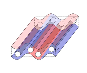
Variations of flow patterns for a simple case of a shear layer modulated by a spanwise temperature pattern with  $\alpha = 1$ and with different disturbance wavenumbers are illustrated in figure 2. The spanwise wavelength of the flow system involves three sets of primary rolls and one set of secondary rolls on the left, and four sets of primary rolls and one set of secondary rolls on the right. Details of this problem, including the notation, are explained later.

Figure 2. (a,b) Primary rolls for  $R{a_{P,L}} = |\bar{g}|\beta {h^3}{\theta _{LP}}/(\kappa \nu ) = 1000,\;Re = {({w_B})_{max}}h/\nu = 2000$ when the shear layer flowing in the z direction is subject to the x modulations of the lower wall temperature with wavenumber $\alpha = 1$. These plots extend over one flow wavelength in the x direction. Colours illustrate the z-velocity component, while the solid black lines illustrate the vector lines in the $(x,y)$ plane. (c,d) Instantaneous iso-surfaces of the disturbance z-velocity component ${w_D}$ over one flow wavelength in the x direction. Iso-surfaces shown correspond to (c) ${w_D} = (2.23, - 2.23)$ and (d) ${w_D} = (1.8, - 1.8)$. The z component of the disturbance wavevector is equal to 1 in both panels; the spanwise component is ${\textstyle{2 \over 3}}$ in (c) and ${\textstyle{1 \over 2}}$ in (d). Red arrows show the locations of hot spots at the lower wall.
Direct numerical simulation can handle only a restrictive class of commensurate systems (Blancher, Le Guer & El Omari Reference Blancher, Le Guer and El Omari2015; Gepner & Floryan Reference Gepner and Floryan2016, Reference Gepner and Floryan2023) as the size of the computational box is limited by the available memory. Continuous change of the disturbance wavenumber is not possible as it results in very large variations of the computational domain, with the stability results being a function of the size of the computational box (Blancher et al. Reference Blancher, Le Guer and El Omari2015; Gepner & Floryan Reference Gepner and Floryan2016, Reference Gepner and Floryan2023). Re-gridding required by changes in the box length represents another significant difficulty due to labour cost. Irrational wavenumber ratios lead to aperiodic incommensurate states, which require an infinite computational box; such states are not accessible to numerical computations due to the inherent truncation error. One may conclude that DNS is suitable for a detailed exploration of particular cases, as the computational cost can be justified; however, it cannot address the stability question in general and is unsuitable for exploring the entire parameter space required for identifying the most effective modulations from either the drag reduction or mixing intensification points of view.
Identifying the most effective modulations requires systematic analysis, which can be accomplished using a process that starts with identifying stationary states, then determining their stability properties, and culminates with establishing saturation states and their domains of attraction. The most promising configurations can then be studied in detail using DNS. This strategy relies on the availability of an accurate stability algorithm that bypasses the limitations of DNS described above.
Stability analysis requires a formulation capable of dealing with various commensurate systems and an accurate numerical method to solve the disturbance equations. The stability of unmodulated shear layers led to the Orr–Sommerfeld equation, whose spectrally accurate solution was given by Orszag (Reference Orszag1971). The formulation of the stability problem, when modulations do not change geometry, was given by Floryan (Reference Floryan1997), who represented disturbance quantities as waves with amplitudes modulated by base flow variations. This formulation avoids the need to use large computational boxes and frees stability results from their dependence on the size of the computational box associated with the use of DNS. Cabal, Szumbarski & Floryan (Reference Cabal, Szumbarski and Floryan2002) implemented this concept in an algorithm that handles modulations associated with surface topographies. This algorithm relied on domain transformation, mapping a complex channel geometry into a smooth slot and using spectral discretization. It is cumbersome to use as it involves very complex field equations. The present work aims to describe a spectrally accurate algorithm that is flexible enough to accurately and efficiently handle a large class of geometric and physical modulations and provide comparison cases that can be used to verify implementations of this algorithm by others, similar to Orszag (Reference Orszag1971). The algorithm uses Fourier expansions in the streamwise and spanwise directions and Chebyshev expansions in the transverse direction coupled with the immersed boundary conditions (IBC) method to handle modulations created by surface topographies.
As the number of possible spatial modulations is uncountable, we present our algorithm in the context of a shear layer modulated by a combination of surface grooves and heating patterns. The latter represents actuations not affecting geometry and are generally simple to implement, and the former represents geometry modulations whose implementation represents a challenge. The generalization of this algorithm to other modulations should not pose a problem as, in all cases, disturbances can be represented as travelling waves with spatially modulated amplitudes. We present detailed convergence studies for selected test problems to provide reliable and accurate comparison data. Special versions of this algorithm were used in the past (Floryan Reference Floryan2002; Hossain & Floryan Reference Hossain and Floryan2013; Moradi & Floryan Reference Moradi and Floryan2014; Mohammadi, Moradi & Floryan Reference Mohammadi, Moradi and Floryan2015; Moradi & Floryan Reference Moradi and Floryan2019), but the underlying concepts are yet to be adequately exposed.
The analysis of the effects of complex topographies requires accurate geometry modelling, as eigenvalues show high sensitivity to minor geometry modifications. Six approaches for handling geometry have been used in the literature. When the groove size is small compared with the overall flow scale, one may argue that it can be accounted for by employing an adequate boundary condition imposed on a smooth surface approximating the actual one (the equivalent surface concept). The implementation details of this concept vary widely (Nye Reference Nye1969; Sarkar & Prosperetti Reference Sarkar and Prosperetti1996; Kamrin, Bazant & Stone Reference Kamrin, Bazant and Stone2010) but can be reduced to a slip boundary condition with the slip parameter adjusted based on numerical experiments (Rothstein Reference Rothstein2010). This concept is unsuitable for stability analysis due to the truncation of flow physics near the corrugated wall.
The second concept takes advantage of small groove amplitude and relies on the boundary conditions transfer procedure, which leads to linearization of the boundary conditions about the mean wall position. Such linearization truncates flow physics as even minor grooves activate nonlinear effects. Including higher-order terms in the transfer procedure (Kamrin et al. Reference Kamrin, Bazant and Stone2010) does not resolve this problem (Cabal, Szumbarski & Floryan Reference Cabal, Szumbarski and Floryan2001). The third method of treating surface topography relies on analytic mappings, which transfer a complex flow geometry into a geometrically regular computational domain. Such mapping leads to a complex form of the field equations whose solution is computationally expensive (Cabal et al. Reference Cabal, Szumbarski and Floryan2002). The fourth concept relies on numerically constructed grids. The available grid generators are only second-order accurate (Geuzaine & Remacle Reference Geuzaine and Remacle2009) – sufficient for work with typical finite-volume discretizations (Moukalled, Mangani & Darwish Reference Moukalled, Mangani and Darwish2015) but insufficient for stability problems. Spectral elements bypass this difficulty, but matching neighbouring elements becomes challenging when deformed geometries are considered (Karniadakis & Sherwin Reference Karniadakis and Sherwin2013; Cantwell et al. Reference Cantwell2015). Accurate grid generation methods providing near-spectral accuracy are available (Floryan Reference Floryan1986; Floryan & Zemach Reference Floryan and Zemach1987, Reference Floryan and Zemach1993) but are cumbersome. The shortcoming of all the above techniques is laborious grid generation whenever a new groove geometry is considered, especially when carrying out grid convergence studies to verify the results. The cost of grid generation limits the use of these methods when an analysis of a large number of geometries is required but makes them very useful when an in-depth analysis of a small number of geometries is needed.
The fifth method relies on the fictitious boundaries concept, whose origins refer to techniques developed to solve moving boundary problems using fixed grids (Floryan & Rasmussen Reference Floryan and Rasmussen1989). Its recent implementations are described in Peskin (Reference Peskin1982, Reference Peskin2002). These methods rely on low-order spatial discretization and local fictitious forces to enforce the no-slip and no-penetration conditions, resulting in truncation of flow physics, which makes them unsuitable for stability analysis. The sixth method combines spectral discretization with the IBC concept. Spectral methods provide the high spatial accuracy required for stability analysis, but their use is limited to regular geometries due to the involvement of global basis functions. This limitation is overcome by the IBC concept (Szumbarski & Floryan Reference Szumbarski and Floryan1999), which relies on the spectrally accurate construction of boundary constraints enforcing flow boundary conditions. The programming effort associated with changing the domain geometry is reduced to the specification of Fourier coefficients describing the groove shape. This method has been extended to moving boundary problems (Husain & Floryan Reference Husain and Floryan2010), and its applicability has been expanded using the over-constrained formulation (Husain, Szumbarski & Floryan Reference Husain, Szumbarski and Floryan2009). The algorithm presented in the paper takes advantage of the IBC method.
The presentation of the stability algorithm and demonstration of its accuracy, efficiency and flexibility are organized into seven parts. Section 2 describes a convenient model problem to focus the presentation of the algorithm. Section 3 briefly discusses the determination of stationary states, the first step in the overall analysis. The linear stability analysis is presented in § 4, with § 4.1 describing the modal equations, § 4.2 discussing the discretization of the boundary conditions and § 4.3 describing the complete discretized system. Section 5 briefly discusses the numerical solution to the eigenvalue problem and tracing procedures. The accuracy testing and demonstration of spectral convergence are described in § 6. Section 7 presents an example of an application problem. Section 8 gives a summary of the main conclusions.
2. Problem formulation
The model problem involves flow between two parallel plates extending to ±∞ in the x and z directions. Distributed heating and surface grooves spatially modulate this flow. We limit this presentation to modulations that are the spanwise x-coordinate functions. The formulation can be easily extended to modulations being functions of the streamwise z coordinate – its details are not presented due to their length. The conduit is oriented in a way where the gravity g works in the negative y-direction (figure 3). The fluid is assumed to be incompressible with the density ρ variations modelled using the Boussinesq approximation; it has thermal conductivity k, specific heat c, thermal diffusivity  $\kappa = k/\rho c$, kinematic viscosity $\nu $, dynamic viscosity $\mu $ and thermal expansion coefficient $\beta $. The non-dimensional equations of motion are
 \begin{align}\boldsymbol{\nabla }\boldsymbol{\cdot }\bar{V} = 0,\quad\! \frac{{\partial \bar{V}}}{{\partial t}} + (\bar{V}\boldsymbol{\cdot }\boldsymbol{\nabla })\bar{V} ={-}\boldsymbol{\nabla }p + {\nabla ^2}\bar{V} + P{r^{ - 1}}\theta \bar{j},\quad\! \frac{{\partial \theta }}{{\partial t}} + (\bar{V}\boldsymbol{\cdot }\boldsymbol{\nabla })\theta = P{r^{ - 1}}{\nabla ^2}\theta ,\end{align}
where half of the channel height h is used as length scale, velocity vector  $\bar{V} = (u\bar{i} + v\bar{j} + w\bar{k})$ is normalized by the viscous velocity scale ${U_v} = v/h$, pressure p is scaled with $\rho U_v^2$, temperature $\theta $ is scaled with $\kappa \nu /(|{g}|\beta {h^3})$, $Pr = v/k$ is the Prandtl number. The relevant boundary conditions are
 \begin{align}\bar{V}[{y_L}(x),t] = \bar{V}[{y_U}(x),t] = 0,\quad \theta [{y_L}(x),t] = {\theta _L}(x,t),\quad \theta [{y_U}(x),t] = {\theta _U}(x,t),\end{align}
where the subscripts L and U refer to the lower and upper plates, respectively, and  ${y_L}(x)$ and ${y_U}(x)$ describe groove geometry.

Figure 3. Schematic diagram of the flow system. Red and blue colours identify hot and cold sections of the walls.
The above system is closed by specifying constraints either in the form of mean pressure gradients in the x and z directions, that is,
 \begin{align}{\left. {\frac{{\partial p}}{{\partial x}}} \right|_{mean}} = {\wp _x},\quad {\left. {\frac{{\partial p}}{{\partial z}}} \right|_{mean}} = {\wp _z},\end{align}
or in the form of the mean flow rates in the x and z directions, that is,
 \begin{equation}{Q_x}{|_{mean}} = {\mathrm{\mathbb{Q}}_x},\quad {Q_z}{|_{mean}} = {\mathrm{\mathbb{Q}}_z}.\end{equation}
In the absence of grooves and heating, the velocity and pressure fields of the reference flow have the form
 \begin{equation}\boldsymbol{V}(x,y,z) = [0,0,w] = [0,\; 0,\; Re(1 - {y^2})],\quad p(x,y,z) ={-} 2\; zRe,\quad {Q_z} = {\textstyle{4 \over 3}}Re,\end{equation}
where the Reynolds number is defined as  $Re = {W_{max}}h/\nu = {W_{max}}/{U_v}$ and ${W_{max}}$ denotes the maximum of the z-velocity component. In the computations, reference flow with a specific Re is selected, and its modified state is determined.
Fourier expansions of the form
 \begin{gather}{y_L}(x) ={-} 1 + {B_L}{Y_L}(x) ={-} 1 + {B_L}\sum\limits_{n ={-} {N_G}}^{n = {N_G}} {H_L^{(n)}\,{\textrm{e}^{\textrm{i}n\alpha x}}} ,\end{gather}
 \begin{gather}{y_U}(x) = 1 + {B_U}{Y_U}(x) = 1 + {B_U}\sum\limits_{n ={-} {N_G}}^{n = {N_G}} {H_U^{(n)}\,{\textrm{e}^{\textrm{i}n(\alpha x + {\varOmega _G})}}}\end{gather}
describe the surface topographies. In the above,  ${Y_L}(x)$ and ${Y_U}(x)$ are the shape functions describing plates’ topographies satisfying conditions
 \begin{equation}\textrm{max}[{Y_L}(x)] - \textrm{min}[{Y_L}(x)] = 1,\quad \textrm{max}[{Y_U}(x)] - \textrm{min}[{Y_U}(x)] = 1,\end{equation} ${B_L}$ and ${B_U}$ are the peak-to-bottom groove amplitudes at the lower and upper plates, respectively, $H_L^{(n)}$ and $H_U^{(n)}$ are the coefficients of the Fourier expansions describing the shape of grooves at the lower and upper plates, respectively, ${N_G}$ is the number of Fourier modes required to describe the geometry, $\alpha $ is the modulation wavenumber and ${\varOmega _G}$ stands for the phase shift between the upper and lower groove systems.
The plates’ temperatures are expressed as Fourier expansions of the form
 \begin{gather}{\theta _L}(x) = R{a_{uni}} + R{a_{P,L}}{\varTheta _L}(x) = R{a_{uni}} + R{a_{P,L}}\sum\limits_{n ={-} {N_L},\;n \ne 0}^{n ={+} {N_L}} {\theta _L^{(n)}\,{\textrm{e}^{\textrm{i}n(\alpha x + {\varOmega _{T,L}})}}} ,\end{gather}
 \begin{gather}{\theta _U}(x) = R{a_{P,U}}{\varTheta _U}(x) = R{a_{P,U}}\sum\limits_{n ={-} {N_L},n \ne 0}^{n ={+} {N_L}} {\theta _U^{(n)}\,{\textrm{e}^{\textrm{i}n(\alpha x + {\varOmega _{T,U}})}}} ,\end{gather}
where  ${\varTheta _L}(x)$ and ${\varTheta _U}(x)$ are the shape functions describing temperature distributions at the lower and upper plates, respectively, satisfying conditions
 \begin{equation}\textrm{max}[{\varTheta _L}(x)] - \textrm{min}[{\varTheta _L}(x)] = 1,\quad \textrm{max}[{\varTheta _U}(x)] - \textrm{min}[{\varTheta _U}(x)] = 1,\end{equation} $\theta _L^{(n)}$ and $\theta _U^{(n)}$ are the coefficients of the Fourier expansions describing the temperature profile at the lower and upper plates, respectively, ${N_L}$ is the number of Fourier modes required to describe the form of heating, $R{a_{uni}} = |{g}|\beta {h^3}{\theta _{uni}}/(\kappa \nu )$ is the uniform Rayleigh number measuring the intensity of the uniform component of heating, $R{a_{P,L}} = |{g}|\beta {h^3}{\theta _{LP}}/(\kappa \nu )$ is the lower periodic Rayleigh number measuring the intensity of the lower periodic heating, $R{a_{P,U}} = |{g}|\beta {h^3}{\theta _{UP}}/(\kappa \nu )$ is the upper periodic Rayleigh number measuring the intensity of the upper periodic heating, ${\theta _{LP}}$ and ${\theta _{UP}}$ are the differences between the maximum and minimum of the lower and upper periodic temperature components, ${\varOmega _{T,L}}$ stands for the phase shift between the lower groove and the lower temperature distribution and ${\varOmega _{T,U}}$ stands for the phase shift between the lower groove and the upper-temperature distribution. We focus on systems with perfectly tuned heating and groove modulations; these modulations are described by the same wavenumber $\alpha $.
The stability problem represents an initial-value problem that can be solved using DNS for any initial disturbance velocity and temperature fields set. The Fourier–Chebyshev expansions combined with IBC method provide the required high-accuracy discretization capable of handling complex geometry (Panday & Floryan Reference Panday and Floryan2020, Reference Panday and Floryan2021). The spectral element method described in Cantwell et al. (Reference Cantwell2015) represents an alternative, but its existing implementations provide only a low-order temporal discretization. The DNS requires the specification of a computational box containing an integer number of modulation wavelengths and an integer number of disturbance wavelengths. Such a box may have to be very long. Its size limits possible investigations to a few combinations of groove and heating wavelengths (Blancher et al. Reference Blancher, Le Guer and El Omari2015; Gepner & Floryan Reference Gepner and Floryan2016, Reference Gepner and Floryan2023) and prevents analysis of arbitrary disturbances. Here, we pursue a strategy that avoids these difficulties. We start with determining stationary states and follow up with their stability analysis to determine onset conditions for secondary states.
The following section briefly discusses the algorithm required for determining stationary states. This algorithm has been described elsewhere (Panday & Floryan Reference Panday and Floryan2020, Reference Panday and Floryan2021), so the presentation is limited to the basic concepts required to describe the stability algorithm.
3. Determination of stationary states
Stationary states are described by the stationary version of (2.1) and (2.2). It is helpful to restate these equations for clarity of the presentation:
 \begin{gather}\boldsymbol{\nabla }\boldsymbol{\cdot }{\bar{V}_B} = 0,\quad ({\bar{V}_B}\boldsymbol{\cdot }\boldsymbol{\nabla }){\bar{V}_B} ={-} \boldsymbol{\nabla }{p_B} + {\nabla ^2}{\bar{V}_B} + P{r^{ - 1}}{\theta _B}\bar{j},\quad ({\bar{V}_B}\boldsymbol{\cdot }\boldsymbol{\nabla }){\theta _B} = P{r^{ - 1}}{\nabla ^2}{\theta _B},\end{gather}
 \begin{gather}{\bar{V}_B}[{y_L}(x)] = {\bar{V}_B}[{y_U}(x)] = 0,\quad {\theta _B}[{y_L}(x)] = {\theta _L}(x),\; \quad {\theta _B}[{y_U}(x)] = {\theta _U}(x),\end{gather}
where subscript B denotes stationary quantities. One needs to add either the pressure gradient constraint  ${\wp _x}$ or the flow rate constraint ${\mathrm{\mathbb{Q}}_x}$ for the x direction, and either the pressure constraint ${\wp _z}$ or the flow rate constraint ${\mathrm{\mathbb{Q}}_z}$ for the z direction. Most of the computations have been carried out with ${\wp _x} = 0$ and ${\wp _z} ={-} 2Re$, where the Reynolds number is defined as $Re = {({w_B})_{max}}h/\nu $.
We use spectrally accurate spatial discretization capable of reducing the discretization error to machine accuracy. This discretization relies on Fourier expansions in the z-streamwise and x-spanwise directions and Chebyshev expansions in the y-transverse direction. The algebraic equations are constructed using the Galerkin projection method. The irregularity of the flow domain is handled using the spectrally accurate IBC method, with flow boundary conditions replaced by constraints implemented using the tau method. Details of the algorithm are given in Panday & Floryan (Reference Panday and Floryan2020).
For simplicity of presentation of the stability algorithm, we express velocity components, pressure and temperature of stationary states in the following form:
 \begin{equation}[{u_B},{v_B},{w_B},{p_B},{\theta _B}](x,y) = \sum\limits_{n ={-} {N_B}}^{{N_B}} {[f_u^{\langle n\rangle },f_v^{\langle n\rangle },f_w^{\langle n\rangle },f_p^{\langle n\rangle },f_\theta ^{\langle n\rangle }](y)\,{\textrm{e}^{\textrm{i}\,n\alpha x}}} .\end{equation}
We have also defined the vorticity vector as
 \begin{equation}{\bar{\omega }_B} = ({\xi _B},{\eta _B},{\phi _B}) = \left( {\frac{{\partial {w_B}}}{{\partial y}} - \frac{{\partial {v_B}}}{{\partial z}},\frac{{\partial {u_B}}}{{\partial z}} - \frac{{\partial {w_B}}}{{\partial x}},\frac{{\partial {v_B}}}{{\partial x}} - \frac{{\partial {u_B}}}{{\partial y}}} \right),\end{equation}
and write its components as Fourier expansions of the form
 \begin{equation}[{\xi _{B,\; }}{\eta _B},{\phi _B}](x,y) = \sum\limits_{n ={-} {N_B}}^{{N_B}} {[f_\xi ^{\langle n\rangle },f_\eta ^{\langle n\rangle },f_\phi ^{\langle n\rangle }](y)\,{\textrm{e}^{\textrm{i}\,n\alpha x}}} .\end{equation}
4. Linear stability analysis
The stability analysis begins with the governing equations expressed in terms of the vorticity transport, energy and continuity equations in the following form:
 \begin{gather}\frac{{\partial \bar{\omega }}}{{\partial t}} - (\bar{\omega }\boldsymbol{\cdot }\boldsymbol{\nabla })\bar{V} + (\bar{V}\boldsymbol{\cdot }\boldsymbol{\nabla })\bar{\omega } = {\nabla ^2}\bar{\omega } + \boldsymbol{\nabla } \times (P{r^{ - 1}}\theta \bar{j}),\quad \frac{{\partial \theta }}{{\partial t}} + (\bar{V}\boldsymbol{\cdot }\boldsymbol{\nabla })\theta = P{r^{ - 1}}{\nabla ^2}\theta ,\end{gather}
 \begin{gather}\boldsymbol{\nabla }\boldsymbol{\cdot }\bar{V} = 0,\quad \bar{\omega } = \boldsymbol{\nabla } \times \bar{V}.\end{gather}
Unsteady three-dimensional disturbances are superposed on the stationary flow in the form
 \begin{align}
\bar{\omega } &= {\bar{\omega }_B}(x,y) + {\bar{\omega
}_D}(x,y,z,t),\quad \bar{V} = {\bar{V}_B}(x,y) +
{\bar{V}_D}(x,y,z,t),\nonumber\\
\theta &= {\theta _B}(x,y) +
{\theta _D}(x,y,z,t),\end{align}
\begin{align}
\bar{\omega } &= {\bar{\omega }_B}(x,y) + {\bar{\omega
}_D}(x,y,z,t),\quad \bar{V} = {\bar{V}_B}(x,y) +
{\bar{V}_D}(x,y,z,t),\nonumber\\
\theta &= {\theta _B}(x,y) +
{\theta _D}(x,y,z,t),\end{align}where subscript D denotes disturbance quantities. The flow quantities (4.2) are substituted into (4.1), the mean parts are subtracted and the equations are linearized, yielding the linear disturbance equations of the form
 \begin{align} &\frac{{\partial {{\bar{\omega }}_D}}}{{\partial t}} - ({\bar{\omega
}_B}\boldsymbol{\cdot }\boldsymbol{\nabla }){\bar{V}_D} -
({\bar{\omega }_D}\boldsymbol{\cdot }\boldsymbol{\nabla
}){\bar{V}_B} + ({\bar{V}_B}\boldsymbol{\cdot
}\boldsymbol{\nabla }){\bar{\omega }_D} +
({\bar{V}_D}\boldsymbol{\cdot }\boldsymbol{\nabla
}){\bar{\omega }_B} \nonumber\\
&\quad = {\nabla ^2}{\bar{\omega }_D} +
\boldsymbol{\nabla } \times (P{r^{ - 1}}{\theta _D}\bar{j}),\end{align}
\begin{align} &\frac{{\partial {{\bar{\omega }}_D}}}{{\partial t}} - ({\bar{\omega
}_B}\boldsymbol{\cdot }\boldsymbol{\nabla }){\bar{V}_D} -
({\bar{\omega }_D}\boldsymbol{\cdot }\boldsymbol{\nabla
}){\bar{V}_B} + ({\bar{V}_B}\boldsymbol{\cdot
}\boldsymbol{\nabla }){\bar{\omega }_D} +
({\bar{V}_D}\boldsymbol{\cdot }\boldsymbol{\nabla
}){\bar{\omega }_B} \nonumber\\
&\quad = {\nabla ^2}{\bar{\omega }_D} +
\boldsymbol{\nabla } \times (P{r^{ - 1}}{\theta _D}\bar{j}),\end{align} \begin{align}&\frac{{\partial {\theta _D}}}{{\partial t}} + ({\bar{V}_B}\boldsymbol{\cdot }\boldsymbol{\nabla }){\theta _D} + ({\bar{V}_D}\boldsymbol{\cdot }\boldsymbol{\nabla }){\theta _B} = P{r^{ - 1}}{\nabla ^2}{\theta _D},\quad \boldsymbol{\nabla }\boldsymbol{\cdot }{\bar{V}_D} = 0,\quad {\bar{\omega }_D} = \boldsymbol{\nabla } \times {\bar{V}_D}.\end{align}
The homogeneous boundary conditions of the form
 \begin{equation}{\bar{V}_D}(x,y,z,t) = 0,\quad {\theta _D}(x,y,z,t) = 0\quad \textrm{at}\;y = {y_L}(x)\textrm{ and }y = {y_U}(x)\end{equation}
complete the formulation.
The solution of (4.3) can be written as a travelling wave with modulated amplitude, i.e.
 \begin{equation}[{\bar{V}_D},{\bar{\omega }_D},{\theta _D}](x,y,z,t) = [{\bar{G}_D},{\bar{\varOmega }_D},{\kappa _D}](x,y)\,{\textrm{e}^{\textrm{i}(\delta x + \mu z - \sigma t)}} + \textrm{c}\textrm{.c}\textrm{.},\end{equation}
where δ and μ are the real wavenumbers in the x and z directions, respectively, representing components of the disturbance wavevector,  $\sigma = {\sigma _r} + \textrm{i}{\sigma _i}$ is the complex frequency with ${\sigma _i}$ describing the rate of growth of disturbances and ${\sigma _r}$ describing their frequency and c.c. stands for the complex conjugate. Functions ${\bar{G}_D}(x,y)$, ${\bar{\varOmega }_D}(x,y)$ and ${\kappa _D}(x,y)$ are the x-periodic amplitude functions accounting for the groove and heating-induced modulations. Substituting (4.5) into (4.3) leads to partial differential equations for the amplitude functions. Since these functions are x-periodic, they can be expressed in terms of the Fourier expansions of the form
 \begin{gather}{\bar{G}_D}(x,y) = \sum\limits_{m ={-} {N_D}}^{ + {N_D}} {[g_u^{\langle m\rangle }(y),g_v^{\langle m\rangle }(y),g_w^{\langle m\rangle }(y)]\,{\textrm{e}^{\textrm{i}\,m\alpha x}}} + \textrm{c}\textrm{.c}\textrm{.},\end{gather}
 \begin{gather}{\bar{\varOmega }_D}(x,y) = \sum\limits_{m ={-} {N_D}}^{ + {N_D}} {[g_\xi ^{\langle m\rangle }(y),g_\eta ^{\langle m\rangle }(y),g_\phi ^{\langle m\rangle }(y)]\,{\textrm{e}^{\textrm{i}\,m\alpha x}}} + \textrm{c}\textrm{.c}\textrm{.},\end{gather}
 \begin{gather}{\kappa _D}(x,y) = \sum\limits_{m ={-} {N_D}}^{ + {N_D}} {[g_\theta ^{\langle m\rangle }(y)]\,{\textrm{e}^{\textrm{i}\,m\alpha x}}} + \textrm{c}\textrm{.c}\textrm{.},\end{gather}
where  $g_u^{\langle m\rangle }(y),g_v^{\langle m\rangle }(y),g_w^{\langle m\rangle }(y),g_\xi ^{\langle m\rangle }(y),g_\eta ^{\langle m\rangle }(y),g_\phi ^{\langle m\rangle }(y),g_\theta ^{\langle m\rangle }(y)$ stand for the modal functions.
A combination of (4.5) and (4.6) provides the final expressions for  ${{\bar{V}}_D}$, ${{\bar{\omega }}_D}$ and ${{\theta }_D}$ of the form
 \begin{gather}{\bar{V}_D}(x,y,z,t) = \sum\limits_{m ={-} {N_D}}^{ + {N_D}} {[g_u^{\langle m\rangle }(y),g_v^{\langle m\rangle }(y),g_w^{\langle m\rangle }(y)]\,{\textrm{e}^{\textrm{i}[(\delta + m\alpha )x + \mu z - \sigma t]}}} + \textrm{c}\textrm{.c}\textrm{.},\end{gather}
 \begin{gather}{\bar{\omega }_D}(x,y,z,t) = \sum\limits_{m ={-} {N_D}}^{ + {N_D}} {[g_\xi ^{\langle m\rangle }(y),g_\eta ^{\langle m\rangle }(y),g_\phi ^{\langle m\rangle }(y)]\,{\textrm{e}^{\textrm{i}[(\delta + m\alpha )x + \mu z - \sigma t]}}} + \textrm{c}\textrm{.c}\textrm{.},\end{gather}
 \begin{gather}{\theta _D}(x,y,z,t) = \sum\limits_{m ={-} {N_D}}^{ + {N_D}} {[g_\theta ^{\langle m\rangle }(y)]\,{\textrm{e}^{\textrm{i}[(\delta + m\alpha )x + \mu z - \sigma t]}}} + \textrm{c}\textrm{.c}\textrm{.}\end{gather}
The above formulation provides means for analysis of the effects of continuous variations of the disturbance wavenumbers δ and μ for a specific modulation wavenumber  $\alpha $, i.e. requires a computational box of the same size as the box used to determine the stationary state.
Substitution of (4.7) into (4.3) leads to  $(2{N_D} + 1)$ ordinary differential equations (ODEs) for the unknown modal functions for each partial differential equation in the above system. Separation of Fourier modes and extensive rearrangements provide an explicit form of these ODEs expressed in terms of $g_v^{\langle m\rangle },g_\eta ^{\langle m\rangle },g_\theta ^{\langle m\rangle }$ suitable for computations, i.e.
 \begin{gather}{T^{\langle m\rangle }}g_v^{\langle m\rangle } - P{r^{ -
1}}k_m^2g_\theta ^{\langle m\rangle } = -\sum\limits_{n ={-}
{N_M}}^{{N_M}} [(T_1^{\langle m - n\rangle } +
T_2^{\langle m - n\rangle } + T_3^{\langle m - n\rangle
})g_v^{\langle m - n\rangle }\nonumber\\
+\,(T_4^{\langle m - n\rangle } - T_5^{\langle m - n\rangle
})\; g_\eta ^{\langle m - n\rangle }] ,\end{gather}
\begin{gather}{T^{\langle m\rangle }}g_v^{\langle m\rangle } - P{r^{ -
1}}k_m^2g_\theta ^{\langle m\rangle } = -\sum\limits_{n ={-}
{N_M}}^{{N_M}} [(T_1^{\langle m - n\rangle } +
T_2^{\langle m - n\rangle } + T_3^{\langle m - n\rangle
})g_v^{\langle m - n\rangle }\nonumber\\
+\,(T_4^{\langle m - n\rangle } - T_5^{\langle m - n\rangle
})\; g_\eta ^{\langle m - n\rangle }] ,\end{gather} \begin{gather}\begin{array}{l} {S^{\langle m\rangle }}g_\eta ^{\langle m\rangle } = \sum\limits_{n ={-} {N_M}}^{ + {N_M}} {[(S_1^{\langle m - n\rangle } + S_2^{\langle m - n\rangle } + S_3^{\langle m - n\rangle })g_v^{\langle m - n\rangle } + (S_4^{\langle m - n\rangle } - S_5^{\langle m - n\rangle })g_\eta ^{\langle m - n\rangle }],} \\ \end{array}\end{gather}
 \begin{gather}{Q^{\langle m\rangle }}g_\theta ^{\langle m\rangle } = \sum\limits_{n ={-} {N_M}}^{ + {N_M}} {\left[ {Q_1^{\langle m - n\rangle }g_\theta^{\langle m - n\rangle } + Q_2^{\langle m - n\rangle }g_v^{\langle m - n\rangle } + \frac{{\mu n\alpha f_\theta^{\langle n\rangle }}}{{k_{m - n}^2}}g_\eta^{\langle m - n\rangle }} \right]} ,\end{gather}
where all operators used in the above expressions are defined in Appendix A. The right-hand sides provide modulation-imposed coupling between different modes. The coupling terms contain indices  $\langle m - n\rangle$ with the relevant terms truncated for $|m - n|\ge {N_D}$.
The boundary conditions can be written as
 \begin{equation}\sum\limits_{m ={-} {N_D}}^{{N_D}} {[g_u^{\langle m\rangle },\; g_v^{\langle m\rangle },\; \; g_w^{\langle m\rangle },\; \; g_\theta ^{\langle m\rangle }]\,{\textrm{e}^{\textrm{i}\,m\alpha x}}} = 0\quad \textrm{at}\;y = {y_L}(x)\textrm{ and }y = {y_U}(x).\end{equation}
One needs to extract boundary conditions for different Fourier modes. This process is complex due to the irregularity of the flow domain, which provides coupling between different modes. We provide a detailed explanation in § 4.2.
In the limit of no modulations, the stationary state is reduced to mode zero of  ${w_B}$ and ${\theta _B}$. The disturbance wavenumber $\delta $ in the x direction is taken as $\alpha $, and the system is reduced after rearranging indices ${t_m} = (m + 1)\alpha = J\alpha $ to the following form:
 \begin{gather}{T^{\langle J\rangle }}g_v^{\langle J\rangle } - P{r^{ - 1}}k_J^2g_\theta ^{\langle J\rangle } + \{ [\textrm{i}\mu {D^2} - \textrm{i}\mu ({D^2} - k_J^2)]f_w^{\left\langle 0 \right\rangle }\} g_v^{\langle J\rangle } = 0,\end{gather}
 \begin{gather}{S^{\langle J\rangle }}g_\eta ^{\langle J\rangle } - i\mu f_w^{\langle 0\rangle }g_\eta ^{\langle J\rangle } + \textrm{i}J\alpha Df_w^{\langle 0\rangle }g_v^{\langle J\rangle } = 0,\end{gather}
 \begin{gather}{Q^{\langle J\rangle }}g_\theta ^{\langle J\rangle } - \textrm{i}\mu f_w^{\langle 0\rangle }g_\theta ^{\langle J\rangle } - Df_\theta ^{\langle 0\rangle }g_v^{\langle J\rangle } = 0,\end{gather}
where  $k_j^2 = {(J\alpha )^2} + {\mu ^2}$ and $|J|= 0,1,2,3, \ldots ,(2{N_D} + 1)$. Equation (4.10a) is the Orr–Sommerfeld operator with thermal coupling term $- P{r^{ - 1}}k_J^2g_\theta ^{\langle J\rangle }$, (4.10b) is the Squire operator, where $\textrm{i}J\alpha Df_w^{\langle 0\rangle }g_v^{\langle J\rangle }$ is the coupling term with the Orr–Sommerfeld operator, and (4.10c) is the energy equation with $Df_\theta ^{\langle 0\rangle }g_v^{\langle J\rangle }$ providing coupling with the Orr–Sommerfeld operator.
4.1. Discretization of the modal equations
Determination of the amplitude functions requires a numerical solution of a system of ODEs described in the previous section. The modal functions are to be represented in terms of Chebyshev expansions. Our preference for the standard definition of the Chebyshev polynomials requires a preliminary mapping of the solution domain  $y \in ( - 1 - {y_b},1 + {y_t})$ onto $\hat{y} \in ( - 1,1)$ using transformation $\hat{y} = \varGamma \textrm{[}y - (1 + {y_t})\textrm{]} + 1$ with $\varGamma = 2/(2 + {y_t} + {y_b})$, where ${y_t}$ and ${y_b}$ identify locations of extremities of the upper and lower walls, respectively. The reader may note that this step is not required when boundary modulations are not present. After transformation, the locations of the walls are specified as
 \begin{align}
{\hat{y}_L}(x) &= 1 - \varGamma (2 + {y_t}) + \varGamma {B_L}\sum\limits_{n
={-} {N_G}}^{n = {N_G}}
{H_L^{(n)}\,{\textrm{e}^{\textrm{i}n\alpha x}}} ,\nonumber\\
{\hat{y}_U}(x) &= 1 - \varGamma {y_t} + \varGamma
{B_U}\sum\limits_{n ={-} {N_G}}^{n = {N_G}}
{H_U^{(n)}\,{\textrm{e}^{\textrm{i}n(\alpha x + {\varOmega
_G})}}} .\end{align}
\begin{align}
{\hat{y}_L}(x) &= 1 - \varGamma (2 + {y_t}) + \varGamma {B_L}\sum\limits_{n
={-} {N_G}}^{n = {N_G}}
{H_L^{(n)}\,{\textrm{e}^{\textrm{i}n\alpha x}}} ,\nonumber\\
{\hat{y}_U}(x) &= 1 - \varGamma {y_t} + \varGamma
{B_U}\sum\limits_{n ={-} {N_G}}^{n = {N_G}}
{H_U^{(n)}\,{\textrm{e}^{\textrm{i}n(\alpha x + {\varOmega
_G})}}} .\end{align}It is convenient to cast them in a shorter form for simplicity of the presentation, i.e.
 \begin{align}{\hat{y}_L}(x)
&= \sum\limits_{n ={-} {N_G}}^{n = {N_G}}
{A_L^{(n)}\,{\textrm{e}^{\textrm{i}n\alpha x}}} ,\quad
A_L^{(0)} = 1 + \varGamma ( - 2 - {y_t} +
{B_L}H_L^{(0)}),\nonumber\\
A_L^{(n)} &= \varGamma
{B_L}H_L^{(n)}\quad \textrm{for}\;n \ne 0,\end{align}
\begin{align}{\hat{y}_L}(x)
&= \sum\limits_{n ={-} {N_G}}^{n = {N_G}}
{A_L^{(n)}\,{\textrm{e}^{\textrm{i}n\alpha x}}} ,\quad
A_L^{(0)} = 1 + \varGamma ( - 2 - {y_t} +
{B_L}H_L^{(0)}),\nonumber\\
A_L^{(n)} &= \varGamma
{B_L}H_L^{(n)}\quad \textrm{for}\;n \ne 0,\end{align} \begin{align}
{\hat{y}_U}(x) &= \sum\limits_{n ={-} {N_G}}^{n = {N_G}}
{A_U^{(n)}\,{\textrm{e}^{\textrm{i}n\alpha x}}} ,\quad \;
A_U^{(0)} = 1 + \varGamma ( - {y_t} + {B_U}H_U^{(0)}),\nonumber\\
A_U^{(n)} &= \varGamma {B_U}H_U^{(n)}\quad \textrm{for}\;n
\ne 0.\end{align}
\begin{align}
{\hat{y}_U}(x) &= \sum\limits_{n ={-} {N_G}}^{n = {N_G}}
{A_U^{(n)}\,{\textrm{e}^{\textrm{i}n\alpha x}}} ,\quad \;
A_U^{(0)} = 1 + \varGamma ( - {y_t} + {B_U}H_U^{(0)}),\nonumber\\
A_U^{(n)} &= \varGamma {B_U}H_U^{(n)}\quad \textrm{for}\;n
\ne 0.\end{align}
Equation (4.8) expressed in terms of  $\hat{y}$ assumes the following form:
 \begin{gather}
{\check{T}{} ^{\langle m\rangle }}g_v^{\langle m\rangle } -
P{r^{ - 1}}k_m^2 g_\theta ^{\langle m\rangle } = -\sum\limits_{n ={-}{N_M}}^{{N_M}} [(\check{T}{}_1^{\langle m - n\rangle } +
\check{T}{} _2^{\langle m - n\rangle } + \check{T}{} _3^{\langle m - n\rangle }) g_v^{\langle m - n\rangle }\nonumber\\
+\, (\check{T}{} _4^{\langle m - n\rangle } -
\check{T}{} _5^{\langle m - n\rangle })\; g_\eta ^{\langle
m - n\rangle }] ,\;
\end{gather}
\begin{gather}
{\check{T}{} ^{\langle m\rangle }}g_v^{\langle m\rangle } -
P{r^{ - 1}}k_m^2 g_\theta ^{\langle m\rangle } = -\sum\limits_{n ={-}{N_M}}^{{N_M}} [(\check{T}{}_1^{\langle m - n\rangle } +
\check{T}{} _2^{\langle m - n\rangle } + \check{T}{} _3^{\langle m - n\rangle }) g_v^{\langle m - n\rangle }\nonumber\\
+\, (\check{T}{} _4^{\langle m - n\rangle } -
\check{T}{} _5^{\langle m - n\rangle })\; g_\eta ^{\langle
m - n\rangle }] ,\;
\end{gather} \begin{gather}{\check{S}{} ^{\langle m\rangle }}g_\eta ^{\langle m\rangle } = \; \sum \limits_{n ={-} {N_M}}^{ + {N_M}} [(\check{S}{} _1^{\langle m - n\rangle } + \check{S}{} _2^{\langle m - n\rangle } + \check{S}{} _3^{\langle m - n\rangle })g_v^{\langle m - n\rangle } + (\check{S}{} _4^{\langle m - n\rangle } - \check{S}{} _5^{\langle m - n\rangle })g_\eta ^{\langle m - n\rangle }],\end{gather}
 \begin{gather}{\check{Q}{} ^{\langle m\rangle }}g_\theta ^{\langle m\rangle } = \sum\limits_{n ={-} {N_M}}^{ + {N_M}} {\left[ {\check{Q}{}_1^{\langle m - n\rangle }g_\theta^{\langle m - n\rangle } + \check{Q}{}_2^{\langle m - n\rangle }g_v^{\langle m - n\rangle } + \frac{{\mu n\alpha f_\theta^{\langle n\rangle }}}{{k_{m - n}^2}}g_\eta^{\langle m - n\rangle }} \right]} ,\end{gather}
where all operators appearing in (4.12) are defined in Appendix B.
System (4.12) has variable coefficients involving stationary state – in the first step of the numerical solution, these coefficients are represented as Chebyshev expansions of the form
 \begin{equation}[{u_B},{v_B},{w_B}](x,\hat{y}) = \sum\limits_{n ={-} {N_B}}^{{N_B}} {\sum\limits_{r = 0}^{{N_C} - 1} {[G_{u,r}^{\langle n\rangle },\; G_{v,r}^{\langle n\rangle },G_{w,r}^{\langle n\rangle }]{T_r}(\hat{y})\,{\textrm{e}^{\textrm{i}\,n\alpha x}}} } ,\end{equation}
where  $G_{u,r}^{\langle n\rangle },\; G_{v,r}^{\langle n\rangle }\textrm{ and }G_{w,r}^{\langle n\rangle }$ are known. In the second step, the unknown modal functions are expressed in terms of the Chebyshev expansions of the form
 \begin{equation}[g_v^{\langle m\rangle },g_\eta ^{\langle m\rangle },g_\theta ^{\langle m\rangle }](\hat{y}) = \sum\limits_{k = 0}^{{N_T} - 1} {[G_{k,v}^{\langle m\rangle },G_{k,\eta }^{\langle m\rangle },G_{k,\theta }^{\langle m\rangle }]{T_k}(\hat{y})} ,\end{equation}
where  $G_{k,v}^{\langle m\rangle },G_{k,\eta }^{\langle m\rangle }\;\textrm{and}\;G_{k,\theta }^{\langle m\rangle }$ are unknown and are to be determined. Substitution of (4.13) and (4.14) into (4.12) and application of the Galerkin projection method result, after a rather lengthy algebra, in a system of algebraic equations for these coefficients of the following form:
 \begin{gather}\sum\limits_{k
= 0}^{{N_T} - 1} {\{ {A^{\langle m\rangle
}}G_{k,v}^{\langle m\rangle } - {H^{\langle m\rangle
}}G_{k,\theta }^{\langle m\rangle }\} }\nonumber\\
\quad + \sum\limits_{n
={-} {N_M}}^{{N_M}} {\sum\limits_{k = 0}^{{N_T} - 1}
{\sum\limits_{r = 0}^{{N_T} - 1} {\begin{array}{*{20}{c}}
{\sum\{ {P^{\langle m - n\rangle }}}
\end{array}G_{k,v}^{\langle m - n\rangle } + {R^{\langle m
- n\rangle }}G_{k,\eta }^{\langle m - n\rangle }\} } } } =
0,\end{gather}
\begin{gather}\sum\limits_{k
= 0}^{{N_T} - 1} {\{ {A^{\langle m\rangle
}}G_{k,v}^{\langle m\rangle } - {H^{\langle m\rangle
}}G_{k,\theta }^{\langle m\rangle }\} }\nonumber\\
\quad + \sum\limits_{n
={-} {N_M}}^{{N_M}} {\sum\limits_{k = 0}^{{N_T} - 1}
{\sum\limits_{r = 0}^{{N_T} - 1} {\begin{array}{*{20}{c}}
{\sum\{ {P^{\langle m - n\rangle }}}
\end{array}G_{k,v}^{\langle m - n\rangle } + {R^{\langle m
- n\rangle }}G_{k,\eta }^{\langle m - n\rangle }\} } } } =
0,\end{gather} \begin{gather}\sum\limits_{k = 0}^{{N_T} - 1} {{D^{\langle m\rangle }}G_{k,\eta }^{\langle m\rangle }} + \sum\limits_{n ={-} {N_M}}^{{N_M}} {\sum\limits_{k = 0}^{{N_T} - 1} {\sum\limits_{r = 0}^{{N_T} - 1} {\{ {K^{\langle m - n\rangle }}G_{k,v}^{\langle m - n\rangle } + {Q^{\langle m - n\rangle }}G_{k,\eta }^{\langle m - n\rangle }\} } } } = 0,\end{gather}
 \begin{gather}
\sum\limits_{k = 0}^{{N_T} - 1} {{I^{\langle m\rangle }}G_{k,\theta
}^{\langle m\rangle }} + \sum\limits_{n ={-} {N_M}}^{{N_M}}
\sum\limits_{k = 0}^{{N_T} - 1} \sum\limits_{r =
0}^{{N_T} - 1} \{ {U^{\langle m - n\rangle }}G_{k,\theta
}^{\langle m - n\rangle } \nonumber\\
+\, {\textrm{V}^{\langle m - n\rangle }}G_{k,v}^{\langle m - n\rangle } +
{W^{\langle m - n\rangle }}G_{k,\eta }^{\langle m -
n\rangle }\} = 0,\end{gather}
\begin{gather}
\sum\limits_{k = 0}^{{N_T} - 1} {{I^{\langle m\rangle }}G_{k,\theta
}^{\langle m\rangle }} + \sum\limits_{n ={-} {N_M}}^{{N_M}}
\sum\limits_{k = 0}^{{N_T} - 1} \sum\limits_{r =
0}^{{N_T} - 1} \{ {U^{\langle m - n\rangle }}G_{k,\theta
}^{\langle m - n\rangle } \nonumber\\
+\, {\textrm{V}^{\langle m - n\rangle }}G_{k,v}^{\langle m - n\rangle } +
{W^{\langle m - n\rangle }}G_{k,\eta }^{\langle m -
n\rangle }\} = 0,\end{gather}where all operators appearing in (4.15) are defined in Appendix C.
4.2. Discretization of boundary conditions
The discretization of boundary conditions without geometry modulations leads to a standard form of boundary conditions for each modal function. Modulations create coupling between the modal functions – this coupling is different from the coupling provided by the modulations of the field equations discussed previously. The form of these conditions is presented below.
Thermal, no-slip and no-penetration boundary conditions (4.4) at the lower wall are restated as
 \begin{gather}{\bar{V}_D}(x,{\hat{y}_L}(x),z,t) = \sum\limits_{m ={-} {N_D}}^{ + {N_D}} {[g_u^{\langle m\rangle }({{\hat{y}}_L}(x)),g_v^{\langle m\rangle }({{\hat{y}}_L}(x)),g_w^{\langle m\rangle }({{\hat{y}}_L}(x))]\,{\textrm{e}^{\textrm{i}[(\delta + m\alpha )x + \mu z - \sigma t]}}} = 0,\end{gather}
 \begin{gather}{\theta _D}(x,{\hat{y}_L}(x),z,t) = \sum\limits_{m ={-} {N_D}}^{ + {N_D}} {[g_\theta ^{\langle m\rangle }({{\hat{y}}_L}(x))]\,{\textrm{e}^{\textrm{i}[(\delta + m\alpha )x + \mu z - \sigma t]}}} = 0.\end{gather}
To be consistent with the modal equations, they must be expressed using the vertical velocity and vorticity components. Their form is given below:
 \begin{gather}{u_D}[x,{\hat{y}_L}(x),z,t] = \sum \limits_{m ={-} {N_D}}^{{N_D}} \left[ {\frac{{\textrm{i}\varGamma {t_m}}}{{k_m^2}}g_v^{\langle m\rangle }({{\hat{y}}_L}(x)) - \frac{{\textrm{i}\mu }}{{k_m^2}}g_\eta^{\langle m\rangle }({{\hat{y}}_L}(x))} \right]\,{\textrm{e}^{\textrm{i}[(\delta + m\alpha )x + \mu z - \sigma t]}} = 0,\end{gather}
 \begin{gather}{v_D}[x,{\hat{y}_L}(x),z,t] = \sum\limits_{m ={-} {N_D}}^{{N_D}} {g_v^{\langle m\rangle }({{\hat{y}}_L}(x))\,{\textrm{e}^{\textrm{i}[(\delta + m\alpha )x + \mu z - \sigma t]}}} = 0,\end{gather}
 \begin{gather}{w_D}[x,{\hat{y}_L}(x),z,t] = \sum \limits_{m ={-} {N_D}}^{{N_D}} \left[ {\frac{{\textrm{i}\mu \varGamma }}{{k_m^2}}g_v^{\langle m\rangle }({{\hat{y}}_L}(x)) + \frac{{\textrm{i}{t_m}}}{{k_m^2}}g_\eta^{\langle m\rangle }({{\hat{y}}_L}(x))} \right]\,{\textrm{e}^{\textrm{i}[(\delta + m\alpha )x + \mu z - \sigma t]}} = 0,\end{gather}
 \begin{gather}{\theta _D}[x,{\hat{y}_L}(x),z,t] = \sum\limits_{m ={-} {N_D}}^{{N_D}} {g_\theta ^{\langle m\rangle }({{\hat{y}}_L}(x))\,{\textrm{e}^{\textrm{i}[(\delta + m\alpha )x + \mu z - \sigma t]}}} = 0.\end{gather}
Substitution of the Chebyshev expansion (4.14) into (4.17) results in
 \begin{align}&{u_D}[x,{\hat{y}_L}(x),z,t] \nonumber\\
&\quad= \sum\limits_{m ={-} {N_D}}^{{N_D}} {\sum\limits_{k =
0}^{{N_T} - 1} {\left[ {\frac{{\textrm{i}\varGamma
{t_m}}}{{k_m^2}}D{T_k}[{{\hat{y}}_L}(x)]G_{k,v}^{\langle
m\rangle } - \frac{{\textrm{i}\mu
}}{{k_m^2}}{T_k}[{{\hat{y}}_L}(x)]G_{k,\eta }^{\langle
m\rangle }} \right]\,{\textrm{e}^{\textrm{i}[(\delta +
m\alpha )x + \mu z - \sigma t]}}} } = 0,\end{align}
\begin{align}&{u_D}[x,{\hat{y}_L}(x),z,t] \nonumber\\
&\quad= \sum\limits_{m ={-} {N_D}}^{{N_D}} {\sum\limits_{k =
0}^{{N_T} - 1} {\left[ {\frac{{\textrm{i}\varGamma
{t_m}}}{{k_m^2}}D{T_k}[{{\hat{y}}_L}(x)]G_{k,v}^{\langle
m\rangle } - \frac{{\textrm{i}\mu
}}{{k_m^2}}{T_k}[{{\hat{y}}_L}(x)]G_{k,\eta }^{\langle
m\rangle }} \right]\,{\textrm{e}^{\textrm{i}[(\delta +
m\alpha )x + \mu z - \sigma t]}}} } = 0,\end{align} \begin{align}&{v_D}[{x,{{\hat{y}}_L}(x ),z,t} ]= \sum \limits_{m ={-} {N_D}}^{{N_D}} \sum \limits_{k = 0}^{{N_T} - 1} {T_k}[{\hat{y}_L}(x )]G_{k,v}^{\left\langle m \right\rangle }{e^{i[{({\delta + m\alpha } )x + \mu z - \sigma t} ]}} = 0, \end{align}
 \begin{align}&{w_D}[x,{\hat{y}_L}(x),z,t]\nonumber\\
&\quad = \sum\limits_{m ={-} {N_D}}^{{N_D}} {\sum\limits_{k = 0}^{{N_T} - 1} {\left[ {\frac{{\textrm{i}\mu \varGamma }}{{k_m^2}}D{T_k}[{{\hat{y}}_L}(x)]G_{k,v}^{\langle m\rangle } + \frac{{\textrm{i}{t_m}}}{{k_m^2}}{T_k}[{{\hat{y}}_L}(x)]G_{k,\eta }^{\langle m\rangle }} \right]\,{\textrm{e}^{\textrm{i}[(\delta + m\alpha )x + \mu z - \sigma t]}}} } = 0,\end{align}
\begin{align}&{w_D}[x,{\hat{y}_L}(x),z,t]\nonumber\\
&\quad = \sum\limits_{m ={-} {N_D}}^{{N_D}} {\sum\limits_{k = 0}^{{N_T} - 1} {\left[ {\frac{{\textrm{i}\mu \varGamma }}{{k_m^2}}D{T_k}[{{\hat{y}}_L}(x)]G_{k,v}^{\langle m\rangle } + \frac{{\textrm{i}{t_m}}}{{k_m^2}}{T_k}[{{\hat{y}}_L}(x)]G_{k,\eta }^{\langle m\rangle }} \right]\,{\textrm{e}^{\textrm{i}[(\delta + m\alpha )x + \mu z - \sigma t]}}} } = 0,\end{align} \begin{align}&{\theta _D}[x,{\hat{y}_L}(x),z,t] = \sum \limits_{m ={-} {N_D}}^{{N_D}} \sum \limits_{k = 0}^{{N_T} - 1} {T_k}[{\hat{y}_L}(x)]G_{k,\theta }^{\langle m\rangle }\,{\textrm{e}^{\textrm{i}[(\delta + m\alpha )x + \mu z - \sigma t]}} = 0.\end{align}
The above boundary relations involve values of Chebyshev polynomials and their derivatives at the grooved wall. These values represent periodic functions of the x coordinate and, thus, can be expressed in terms of Fourier expansions as follows:
 \begin{equation}{T_k}[{\hat{y}_L}(x)] = \sum\limits_{p ={-} {N_j}}^{{N_j}} {({w_L})_k^{\langle p\rangle }\,{\textrm{e}^{\textrm{i}\,p\alpha x}}} ,\quad D{T_k}[{\hat{y}_L}(x)] = \sum\limits_{p ={-} {N_j}}^{{N_j}} {({d_L})_k^{\langle p\rangle }\,{\textrm{e}^{\textrm{i}\,p\alpha x}}} .\end{equation}
 Appendix D explains the determination of coefficients  ${w_L}$ and ${d_L}$. Substitution of (4.19) into (4.18), extraction of Fourier modes and retention of the first ${N_D}$ modes result in the boundary relations of the form
 \begin{gather}\sum\limits_{p ={-} {N_D}}^{{N_D}} {\sum\limits_{k = 0}^{{N_T} - 1} {\left[ {\frac{{\textrm{i}\varGamma {t_p}}}{{k_p^2}}({d_L})_k^{\langle m - p\rangle }G_{k,v}^{\langle p\rangle } - \frac{{\textrm{i}\mu }}{{k_p^2}}({w_L})_k^{\langle m - p\rangle }G_{k,\eta }^{\langle p\rangle }} \right]} } = 0,\end{gather}
 \begin{gather}\sum\limits_{p ={-} {N_D}}^{{N_D}} {\sum\limits_{k = 0}^{{N_T} - 1} {({w_L})_k^{\langle m - p\rangle }G_{k,v}^{\langle p\rangle }} } = 0,\end{gather}
 \begin{gather}\sum\limits_{p ={-} {N_D}}^{{N_D}} {\sum\limits_{k = 0}^{{N_T} - 1} {\left[ {\frac{{\textrm{i}\mu \varGamma }}{{k_p^2}}({d_L})_k^{\langle m - p\rangle }G_{k,v}^{\langle p\rangle } + \frac{{\textrm{i}{t_p}}}{{k_p^2}}({w_L})_k^{\langle m - p\rangle }G_{k,\eta }^{\langle p\rangle }} \right]} } = 0,\end{gather}
 \begin{gather}\sum\limits_{p ={-} {N_D}}^{{N_D}} {\sum\limits_{k = 0}^{{N_T} - 1} {({w_L})_k^{\langle m - p\rangle }G_{k,\theta }^{\langle p\rangle }} } = 0,\end{gather}
where truncation  $|m - p|\le {N_D}$ is needed to maintain consistency with the modal equations. Increasing the number of retained boundary relations is possible as it improves spatial accuracy but leads to over-constrained formulation (Husain et al. Reference Husain, Szumbarski and Floryan2009). A similar process leads to boundary relations on the upper wall of the form
 \begin{gather}\sum\limits_{p ={-} {N_D}}^{{N_D}} {\sum\limits_{k = 0}^{{N_T} - 1} {\left[ {\frac{{\textrm{i}\varGamma {t_p}}}{{k_p^2}}({d_U})_k^{\langle m - p\rangle }G_{k,v}^{\langle p\rangle } - \frac{{\textrm{i}\mu }}{{k_p^2}}({w_U})_k^{\langle m - p\rangle }G_{k,\eta }^{\langle p\rangle }} \right]} } = 0,\end{gather}
 \begin{gather}\sum\limits_{p ={-} {N_D}}^{{N_D}} {\sum\limits_{k = 0}^{{N_T} - 1} {({w_U})_k^{\langle m - p\rangle }G_{k,v}^{\langle p\rangle }} } = 0, \end{gather}
 \begin{gather}\sum\limits_{p ={-} {N_D}}^{{N_D}} {\sum\limits_{k = 0}^{{N_T} - 1} {\left[ {\frac{{\textrm{i}\mu \varGamma }}{{k_p^2}}({d_U})_k^{\langle m - p\rangle }G_{k,v}^{\langle p\rangle } + \frac{{\textrm{i}{t_p}}}{{k_p^2}}({w_U})_k^{\langle m - p\rangle }G_{k,\eta }^{\langle p\rangle }} \right]} } = 0,\end{gather}
 \begin{gather}\sum\limits_{p ={-} {N_D}}^{{N_D}} {\sum\limits_{k = 0}^{{N_T} - 1} {({w_U})_k^{\langle m - p\rangle }G_{k,\theta }^{\langle p\rangle }} } = 0.\end{gather}
Relations (4.20) and (4.21) provide intermodal coupling associated with the grooves.
4.3. The linear algebraic system
We include boundary relations in the system (4.15) using the Tau method (Canuto et al. Reference Canuto, Hussaini, Quarteroni and Zang1992), i.e. equations corresponding to the highest-order Chebyshev polynomials in each of (4.15) are replaced with the boundary relations (4.20) and (4.21). The linear system used for computations has a simple form:
 \begin{equation}\boldsymbol{\varLambda }x = 0,\end{equation}
where  $\boldsymbol{\varLambda }$ represents the coefficient matrix and x identifies the vector of unknowns. The structure of the coefficient matrix is illustrated in figure 4(a), where the large blocks identified by green lines correspond to different sets of unknowns (i.e. $v,\eta ,\theta $) – the off-diagonal blocks provide coupling between these unknowns. The structure of a single block for v, displayed in figure 4(b), illustrates couplings between Fourier modes with the diagonal subblocks corresponding to a specific modal function and the off-diagonal subblocks providing couplings between the modes. Rows with green shading identify positions of boundary relations that provide additional intermodal coupling.

Figure 4. (a) Structure of the coefficient matrix  $\boldsymbol{\varLambda }$ for ${N_D} = 2$ and ${N_T} = 10$. Green lines identify off-diagonal blocks providing coupling between different unknowns. (b) Structure of a single block with green shading identifying entries corresponding to boundary relations. Black symbols mark the non-zero elements.
5. Method of solution
A homogeneous system (4.22) has a non-trivial solution only for certain combinations of parameters that are interrelated through a dispersion relation of the form
 \begin{equation}\varTheta \textrm{(}\alpha ,\mu ,\delta ,\sigma ,Re,R{a_{uni}},R{a_{P,L}},R{a_{P,U}},Pr,{B_L},{B_U},H_L^{(n)},H_U^{(n)},\theta _L^{(n)},\theta _U^{(n)}\textrm{)} = 0.\end{equation}
All but two real quantities can be selected arbitrarily. Determining these two quantities requires finding zeros of (5.1). The explicit form of (5.1) is not given. The dispersion relation can be posed in various ways for computational purposes. The first form involves posing the system as an algebraic eigenvalue problem for  $\sigma $ in the form
 \begin{equation}\boldsymbol{AE} = \sigma \boldsymbol{BE},\end{equation}
where  $\boldsymbol{E}$ denotes the eigenvector and $\boldsymbol{A}$ and $\boldsymbol{B}$ are the coefficient matrices. The $\sigma $-spectrum can be computed using a general eigenvalue solver (Moler Reference Moler2004). This process can be computationally expensive, and the computed spectrum may suffer from accuracy problems as our stability problem leads to large algebraic systems. The cost can be reduced by evaluating only a spectrum segment using the Arnoldi method (Saad Reference Saad2003). All these methods are suitable for locating eigenvalues of interest but unsuitable for their tracing through parameter space.
Local solutions are more computationally efficient and accurate but typically produce just one eigenvalue (Moler Reference Moler2004). The first method used in this study, the inverse iterations method (Demmel Reference Demmel1997), is suitable for tracing complex frequencies. One starts with an initial approximation for the eigenpair  $({\boldsymbol{E}_p},{\sigma _p}) = ({\boldsymbol{E}^{(0)}},{\sigma _0})$ and improve it iteratively. The iteration process uses the following relation:
 \begin{equation}(\boldsymbol{A} - {\sigma _0}\boldsymbol{B}){\boldsymbol{E}^{(b + 1)}} = \boldsymbol{B}{\boldsymbol{E}^{(b)}},\end{equation}
which starts with  $b = 0$ and determines the next approximation for the eigenpair as
 \begin{equation}\sigma _p^{(b + 1)} = \boldsymbol{E}_p^{(b)T}\boldsymbol{AE}_p^{(b)}/\boldsymbol{E}_p^{(b)\ast }\boldsymbol{BE}_p^{(b)},\end{equation}
where the asterisk denotes the complex conjugate transpose. If  ${\sigma _p}$ is the eigenvalue closest to ${\sigma _0}$, then ${\boldsymbol{E}^{(b)}}$ converges to ${\boldsymbol{E}_p}$. The initial approximation ${\boldsymbol{E}^{(0)}}$ must be consistent with boundary conditions.
The Newton–Raphson method posed either in terms of one complex variable or in terms of two real variables offers various alternatives. Search for zeros of the determinant of  $\boldsymbol{\varLambda }$ is one of them. This method is ineffective as the determinant varies by several orders of magnitude as a function of the unknown eigenvalue, which leads to numerical difficulties. The alternative approach involves converting the homogeneous problem (4.22) into an inhomogeneous one. To do so, one replaces a homogeneous boundary condition with an inhomogeneous condition, making the system inhomogeneous and easy to solve. The omitted homogeneous boundary condition provides a test verifying if the correct eigenvalue has been selected. This process involves a search for zero of the omitted boundary condition. A simple example of this process in the case of a smooth surface consists of replacing the homogeneous boundary condition for $D{v^{(1)}} = 0$ at one of the walls with an inhomogeneous condition ${D^2}{v^{(1)}} = 1$, which, at the same time, imposes the normalization condition. In general, $D{v^{(1)}}$ is not zero, so one must implement the Newton–Raphson search process to find eigenvalues that bring this condition to zero. Any boundary relation can be used as the test condition. A good initial guess is required to achieve convergence.
6. Testing of the algorithm
The main feature of the algorithm is its high (spectral) accuracy, ability to handle arbitrary temperature and groove patterns very efficiently and ability to handle arbitrary disturbance wavenumbers for any modulation wavenumber. The stationary states were determined using the algorithm described in Panday & Floryan (Reference Panday and Floryan2020). In the tests, the stationary solutions were determined with machine accuracy to eliminate any numerical error in the determinations of these solutions, which may affect the accuracy of stability results.
All the tests reported here have been carried out with zero-pressure-gradient constraints in the x direction. The surface and thermal patterns were of the form
 \begin{align}\left. {\begin{array}{@{}c@{}} {{y_L} ={-} 1 + \dfrac{{{B_L}}}{2}\textrm{cos}(\alpha x),\quad {y_U} ={+} 1,\quad {\theta_L} = R{a_{uni}} + \dfrac{{R{a_{P,L}}}}{2}\textrm{cos}(\alpha x + {\varOmega_{T,L}})\quad \textrm{and}}\\ {{\theta_U} = \dfrac{{R{a_{P,U}}}}{2}\textrm{cos(}\alpha x + {\varOmega_{T,U}}\textrm{)}\textrm{.}} \end{array}} \right\}\end{align}
The tests dealt with (i) two-dimensional disturbances  $(\delta = 0)$ and (ii) three-dimensional disturbances $(\delta \ne 0,\; \mu \ne 0)$.
The algorithm reproduced results for special limiting cases available in the literature (Rayleigh Reference Rayleigh1916; Orszag Reference Orszag1971; Schmid & Henningson Reference Schmid and Henningson2001; Hossain & Floryan Reference Hossain and Floryan2013; Moradi & Floryan Reference Moradi and Floryan2014, Reference Moradi and Floryan2019; Mohammadi et al. Reference Mohammadi, Moradi and Floryan2015).
We provide detailed testing and demonstration of the accuracy of evaluating stability characteristics for flows through a slot formed by grooved walls exposed to periodic heating. The typical spectrum is presented in figure 5, with its width depending on the number of Fourier modes  $({N_D})$ used in the computation. There is one unstable eigenvalue for these conditions $({\sigma _r} + \textrm{i}{\sigma _i}) = (458.6385,\; 7.6468)$, which connects to the Squire spectrum in the limit of no modulations.

Figure 5. (a) Spectrum for flow in a channel with longitudinal grooves exposed to spanwise periodic heating with  $\alpha = 1$, $\delta = 0.8$, $\mu = 0.5$, $R{a_{P,L}} = 500$, ${\varOmega _{T,L}} = {\rm \pi}/2$, ${B_L} = 0.1$, ${B_U} = 0$, $Re = 1000$. Here ${N_D} = 10$ Fourier modes and ${N_T = 120}$ Chebyshev polynomials were used in the test. The leading mode is identified with a square box. (b) Variations of ${\sigma _i}$ of the leading mode as a function of $R{a_{P,L}}$ for grooved surfaces with ${B_L} = 0.2$ (black colour) with $R{a_{P,L}}$ decreasing to zero and then as a function of ${B_L}$ for isothermal surface (blue colour) with ${B_L}$ decreasing to zero.
The accuracy of the determination of the unstable eigenvalue depends on the number of Fourier modes and Chebyshev polynomials used in the computations. In this testing, the stationary state was determined with machine accuracy, so its accuracy does not affect the stability results. We define error  $\mathrm{\Delta }{\sigma _i}$ in the determination of the eigenvalue as
 \begin{equation}\mathrm{\Delta }{\sigma _i} = |{\sigma _i} - {\sigma _{i,ref}}|,\end{equation}
where  ${\sigma _i}$ stands for the computed imaginary part of the eigenvalue and ${\sigma _{i,ref}}$ is its actual value. Since the actual eigenvalue is not known, ${\sigma _{i,ref}}$ has been determined with machine accuracy, which, for the conditions in this test, required the use of ${N_D} = 25$ Fourier modes and ${N_T} = 80$ Chebyshev polynomials.
Figure 6 illustrates variations of  $\mathrm{\Delta }{\sigma _i}$ as a function of the number of Fourier modes ${N_D}$ used in the computations. These tests used ${N_T} = 80$ Chebyshev polynomials to reduce this part of discretization error to the machine level. Results for two-dimensional travelling waves show an exponential decrease of the error as the number of Fourier modes increases, demonstrating the spectral accuracy of the algorithm (figure 6a). The absolute value of the error increases with an increase in the heating intensity; however, the character of its exponential decrease is not affected. A similar exponential reduction of error can be observed for the three-dimensional disturbances in figure 6(b). These results indicate that a near machine accuracy can be achieved using ${N_D} = 15$ Fourier modes.

Figure 6. Variations of the error  $\mathrm{\Delta }{\sigma _i}$ in the evaluation of the amplification rate ${\sigma _i}$ as a function of the number of Fourier modes ${N_D}$ used in the computations for (a) a two-dimensional travelling wave disturbance $({\delta = 0},\; {\mu = 0.3})$ for $\alpha = 1$, ${B_L} = 0.07,{B_U} = 0$, $Re = 1000$ and (b) a three-dimensional travelling wave disturbance $(\delta = 0.8,\; \mu = 0.5)$ for $\alpha = 1$, ${B_L} = 0.1,{B_U} = 0,{\varOmega _{T,L}} = {\rm \pi}/2,\delta = 0.8,\mu = 0.5$. The heating conditions used in the tests were $R{a_{uni}} = 0$ and $R{a_{P,L}} = R{a_{P,U}} = 50$ and $R{a_{P,L}} = R{a_{P,U}} = 75$. All results were obtained with ${N_T} = 80$ Chebyshev polynomials.
Results displayed in figure 7 illustrate variations of  $\mathrm{\Delta }{\sigma _i}$ as a function of the number ${N_T}$ of Chebyshev polynomials used in the computations. These computations used ${N_D = 20}$ Fourier modes to reduce the error associated with this part of discretization to the machine level. The results demonstrate an exponential decrease in the error as the number of Chebyshev polynomials increases. They also illustrate the need to use more Chebyshev polynomials in the case of three-dimensional waves to achieve the same absolute accuracy as in the case of two-dimensional waves. In most cases, 40 Chebyshev polynomials were sufficient to achieve machine accuracy.

Figure 7. Variation of  $\mathrm{\Delta }{\sigma _i}$ as a function of the number of Chebyshev polynomials ${N_T}$ for $\alpha = 1$, ${B_L = 0.07},{B_U = 0},{Re = 500}$ for (a) two-dimensional disturbance with $\delta = 0,\mu = 0.4$ and (b) three-dimensional disturbance with $\delta = 0.4,\mu = 0.4$. The heating conditions used in the tests were $R{a_{uni}} = 0$ and $(R{a_{P,L}},R{a_{P,U}}) = (100,\; 0)$ and $(R{a_{P,L}},R{a_{P,U}}) = (200,\; 200)$. All results were obtained with ${N_D} = 20$ Fourier modes.
The IBC method raises the question of how well the homogeneous boundary conditions are enforced at the grooved walls. Since the expected values of the disturbance velocity components and the disturbance temperature are zero, these quantities evaluated at the boundaries represent the absolute errors. They vary in an oscillatory manner along the wall, as illustrated in figure 8. The relative position of the groove and heating patterns determines the location of the maximum error, but the absolute value of the error is never higher than  ${10^{ - 10}}$.

Figure 8. Distributions of  ${u_D}$ (dash-dotted line), ${v_D}$ (solid line), ${w_D}$ (dashed line) and ${\theta _D}$ (dotted line) at the lower wall for $\alpha = 1$, ${B_L} = 0.07$, ${B_U} = 0$, $Re = 1000$, $R{a_{P,L}} = 100$, $R{a_{P,U}} = 0$, $R{a_{uni}} = 0$, $\mu = 0.4$ and (a) $\delta = 0$ and (b) $\delta = 0.4$. All results were obtained with ${N_D} = 15$ Fourier modes and ${N_T} = 40$ Chebyshev polynomials.
To quantify the boundary error and its variations as a function of the number of Fourier modes, we measured this error using the norm defined as
 \begin{equation}\parallel\!BE\!\parallel\, = \textrm{max}(q){|_{{y_L}}},\end{equation}
where q is the flow quantity of interest. Eigenfunctions used in (6.3) were normalized by bringing their Euclidean norm defined as
 \begin{equation}\Vert\boldsymbol{E}\Vert_{2} = \sqrt {\boldsymbol{E}_1^2 + \boldsymbol{E}_2^2 + \cdots + \boldsymbol{E}_{3{N_T}(2{N_D} + 1)}^2} = 1\end{equation}
to unity. Here  $\boldsymbol{E}$ is an eigenvector that includes each disturbance quantity appearing in (6.3) with length $3{N_T}(2{N_D} + 1)$. Results displayed in figure 9 demonstrate that ${\parallel} BE\parallel $ decreases exponentially with ${N_D}$. The convergence rate varies between different disturbance quantities, but all have exponential forms.

Figure 9. Variations of the boundary errors as functions of the number  ${N_D}$ of Fourier modes used in the computations for $\alpha = 1$, ${B_L} = 0.07$, $Re = 1000$, $R{a_{P,L}} = 100$, $\mu = 0.4$ and (a) $\delta = 0$ and (b) $\delta = 0.4$. All results were obtained with ${N_T} = 80$ Chebyshev polynomials.
Another way to demonstrate the spectral convergence of the algorithm is to determine variations of the Chebyshev norm defined as
 \begin{equation}\Vert \varPhi _q^{(m)}(\hat{y})\Vert = {\left\{ {\int_{ - 1}^1 {G_{k,q}^{(m)}(\hat{y})\; \overline {G_{k,q}^{( - m)}(\hat{y})} \omega (\hat{y})\,\textrm{d}\hat{y}} } \right\}^{1/2}},\end{equation}
where q stands for the modal function of choice. Figure 10 illustrates variations of this norm with an increase of the mode number m for two-dimensional and three-dimensional disturbances. These results confirm the exponential reduction of the Chebyshev norm as the mode number increases for all the quantities.

Figure 10. Variations of the Chebyshev norms as functions of the mode number for  $\alpha = 1$, ${B_L} = 0.07$, ${B_U} = 0$, $Re = 1000$, $R{a_{P,L}} = 100$, $R{a_{P,U}} = R{a_{uni}} = 0$, $\mu = 0.4$ and (a) $\delta = 0$ and (b) $\delta = 0.4$. All results were obtained with ${N_D} = 15$ Fourier modes and ${N_T} = 80$ Chebyshev polynomials.
All the tests reported in this section validate the spectral accuracy of the algorithm. The algorithm has a significant advantage in efficiently handling variations of geometry and heating patterns compared with the grid-based approaches. Its gridless nature makes it suitable for a parametric study involving the analysis of any parameter that defines geometric and heating patterns. Mesh construction and grid independence studies required by analyses using the conventional grid methods are very labour- and time-expensive.
Tables 1 and 2 provide numerical values illustrating the convergence of the test eigenvalue determined using different numbers of Chebyshev polynomials and Fourier modes. The comparison dataset uses a form similar to that of Orszag (Reference Orszag1971), which others can use for verification of the accuracy of their results.
Table 1. Variations of the leading eigenvalue  $\sigma $ as a function of the number of Fourier modes ${N_M}$ and the number of Chebyshev polynomials ${N_T}$ used in the computations for an isothermal system with $R{a_{pL}} = 0$, ${B_L} = 0.1$, ${B_U} = 0$, $\alpha = 1$, $\delta = 0$ and $Re = 3000$, $\mu = 0.4$, and $Re = 7000$, $\mu = 1$.

Table 2. Variations of the leading eigenvalue  $\sigma $ as a function of the number of Fourier modes ${N_M}$ and the number of Chebyshev polynomials ${N_T}$ used in the computations for a non-isothermal system with $Re = 1000$, $R{a_{pL}} = 500$, ${B_L} = 0.1$, ${B_U} = 0$, $\alpha = 1$, $\delta = 0.8$.

7. Example of an application problem
This section discusses an application problem selected to illustrate the capabilities of the proposed algorithm. This problem cannot be convincingly analysed using the DNS-type methodology.
Consider isothermal pressure-gradient-driven flow in a channel modified by longitudinal grooves. This flow is subject to a new type of instability, which, for simplicity, we refer to as Floryan's instability (Mohammadi et al. Reference Mohammadi, Moradi and Floryan2015). The presence of longitudinal grooves creates spanwise gradients of the streamwise velocity, which activate inflection-point-type inviscid instability. The critical Reynolds number can be as low as O(10) if grooves with large enough amplitudes are used (Gepner & Floryan Reference Gepner and Floryan2020). The instability creates waves with phase speed near the maximum flow velocity, leading to laminar chaos in the saturation state (Gepner & Floryan Reference Gepner and Floryan2020). Use of grooves with amplitude  ${B_L} = 0.1$ results in a critical Reynolds number of about $2600$ (see figure 11a). If one adds heating with amplitude $R{a_{P,L}} = 700$ and wavenumber matching the groove wavenumber, and places this heating in such a manner so that hot spots overlap with the groove peaks, e.g. ${\varOmega _{T,L}} = 0$, the critical Reynolds number is reduced to about 375 (see figure 11b). It is thus possible to achieve low critical Re with much smaller groove amplitudes. The use of heating patterns is attractive as heating can be turned on and off as required, and its implementation is likely more economically effective as the creation of special conduit geometries is avoided. Figure 12(a) displays the spectrum for $Re = 400$, which shows the presence of a single unstable eigenvalue. Figure 12(b) illustrates variations in the amplification rate ${\sigma _i}$ as a function of the streamwise wavenumber $\delta $, which is essential for determining $\delta $ giving the largest amplification, this step being required in a stability analysis. Table 3 gives spanwise size W of the computational domain that needs to be used for DNS to reproduce some of these results – this table illustrates difficulties associated with using DNS.

Figure 11. The neutral curves in the  $(Re,\mu )$ plane for flow in (a) an isothermal $(R{a_{P,L}} = R{a_{P,U}} = 0)$ grooved ( $\alpha = 1$, ${B_L} = 0.1$, ${B_U} = 0$) channel for $\delta = 1$ and (b) the same channel heated from below ( $R{a_{P,L}} = 700$, $R{a_{P,U}} = 0$).

Figure 12. (a) Spectrum for flow in a grooved channel exposed to periodic heating for  $\alpha = 1$, $R{a_{P,L}} = 700$, $Re = 400$, ${\varOmega _{T,L}} = 0$, ${B_L} = 0.1$, ${B_U} = 0$ and $\delta = 1$, $\mu = 1$ determined using ${N_D} = 10$ Fourier modes and ${N_T} = 120$ Chebyshev polynomials. (b) Variation of the amplification rate ${\sigma _i}$ as a function of $\delta $ for $\mu = 1$ with other conditions as in (a).
Table 3. Spanwise extent W of the computational domain required for the use of the DNS approach for the heating wavenumber  $\alpha = 1$ and selected disturbance wavenumbers $\delta $.
8. Summary
An algorithm suitable for analysing the stability of spatially modulated shear layers has been proposed and described in the context of modulations induced by surface topography and modulations created by heating patterns. The former represents geometry modulations, while the latter represents field modulations. The algorithm can be easily extended to other forms of modulations. Spatial modulation problems are characterized by the formation of commensurate and incommensurate states arising out of the need to analyse all possible disturbances, and these states are not accessible to classical DNS-based approaches. The proposed algorithm bypasses this problem by treating disturbances as modulated waves and focusing on determining the amplitude functions. This determination relies on spatial discretization based on Fourier expansions in the streamwise and spanwise directions and Chebyshev expansions in the wall-normal direction. The Galerkin projection method has been used to develop the linear system of algebraic equations for the expansion coefficients. The homogeneous boundary conditions to be imposed along the corrugated walls have been replaced by constraints (the IBC method) included in the complete system of linear equations using the Tau concept. The resulting eigenvalue problem was solved using standard methods. Numerous tests demonstrated that the algorithm provides spectral accuracy. Detailed comparison tables for selected test cases have been provided, and the eigenvalue accuracy has been demonstrated. An example of a physical problem was presented to illustrate the power and effectiveness of the proposed method.
The proposed algorithm is gridless and requires minimal user time to adapt to new geometries of the bounding walls and new heating patterns. It bypasses the need for cumbersome grid convergence studies to verify grid-based methods’ accuracy. The number of Fourier modes and Chebyshev polynomials used in the computations sets the absolute accuracy.
Funding
This work has been carried out with support from NSERC of Canada.
Declaration of interests
The authors report no conflict of interest.
Appendix A. Operators used in the system (4.8)
 \begin{gather} t_m = \delta + m\alpha, \end{gather}
 \begin{gather} k_m^2 = t_m^2 + \mu^2, \end{gather}
 \begin{gather} {D^q} = \frac{{{d^q}}}{{d{y^q}}}, \end{gather}
 \begin{gather}{T^{\langle m\rangle }} = {({D^2} - k_m^2)^2} + \textrm{i}\sigma ({D^2} - k_m^2),\end{gather}
 \begin{gather}{S^{\langle m\rangle }} = ({D^2} - k_m^2) + \textrm{i}\sigma ,\end{gather}
 \begin{gather}{Q^{\langle m\rangle }} = P{r^{ - 1}}({D^2} - k_m^2) + \textrm{i}\sigma ,\end{gather}
 \begin{gather}\begin{aligned} T_1^{\langle m - n\rangle } & = \dfrac{{\textrm{i}{t_{m - n}}}}{{k_{m - n}^2}}( - t_m^2Df_u^{\langle n\rangle }D + \textrm{i}n\alpha k_m^2\,f_v^{\langle n\rangle }D - t_m^2\,f_u^{\langle n\rangle }{D^2} + \textrm{i}{t_m}Df_v^{\langle n\rangle }{D^2}\\ & \quad + \textrm{i}{t_m}\,f_v^{\langle n\rangle }{D^3} - 2\mu n\alpha Df_w^{\langle n\rangle }D - \mu {t_{m + n}}\,f_w^{\langle n\rangle }{D^2}), \end{aligned}\end{gather}
 \begin{gather}T_2^{\langle m - n\rangle } \,{=}\, \textrm{i}k_m^2{t_{m - n}}\,f_u^{\langle n\rangle } + k_m^2Df_v^{\langle n\rangle } + k_m^2\,f_v^{\langle n\rangle }D + \textrm{i}{t_m}{D^2}f_u^{\langle n\rangle } + \textrm{i}{t_m}Df_u^{\langle n\rangle }D + \textrm{i}\mu ({D^2} + k_m^2)f_w^{\langle n\rangle },\end{gather}
 \begin{gather}T_3^{\langle m - n\rangle } = \frac{{\textrm{i}\mu }}{{k_{m - n}^2}}( - \mu {t_{m - 2n}}\,f_u^{\langle n\rangle }{D^2} + \textrm{i}\mu f_v^{\langle n\rangle }{D^3} - \mu {t_{m - n}}Df_u^{\langle n\rangle }D - {\mu ^2}f_w^{\langle n\rangle }{D^2}),\end{gather}
 \begin{gather}T_4^{\langle m - n\rangle } = \frac{{\textrm{i}{t_{m - n}}}}{{k_{m - n}^2}}( - \mu {t_{m - 2n}}\,f_u^{\langle n\rangle }D + \textrm{i}\mu f_v^{\langle n\rangle }{D^2} - \mu {t_{m - n}}Df_u^{\langle n\rangle } - {\mu ^2}f_w^{\langle n\rangle }D),\end{gather}
 \begin{gather}\begin{aligned} T_5^{\langle m - n\rangle } & = \dfrac{{\textrm{i}\mu }}{{k_{m - n}^2}}( - t_m^2Df_u^{\langle n\rangle } + \textrm{i}n\alpha k_m^2\,f_v^{\langle n\rangle } - t_m^2\,f_u^{\langle n\rangle }D + \textrm{i}{t_m}Df_v^{\langle n\rangle }D\\ & \quad + \textrm{i}{t_m}\,f_v^{\langle n\rangle }{D^2} - 2\mu n\alpha \; Df_w^{\langle n\rangle } - \mu {t_{m + n}}\,f_w^{\langle n\rangle }D), \end{aligned}\end{gather}
 \begin{gather}S_1^{\langle m - n\rangle } = \frac{{\textrm{i}\mu }}{{k_{m - n}^2}}({t_{m - n}}{t_m}\,f_u^{\langle n\rangle }D - \textrm{i}{t_m}\,f_v^{\langle n\rangle }{D^2} + \mu {t_{m - n}}\,f_w^{\langle n\rangle }D),\end{gather}
 \begin{gather}S_2^{\langle m - n\rangle } = \textrm{i}\mu Df_u^{\langle n\rangle } - \textrm{i}{t_{m - n}}Df_w^{\langle n\rangle } + \textrm{i}n\alpha \; f_w^{\langle n\rangle }D - \textrm{i}n\alpha Df_w^{\langle n\rangle },\end{gather}
 \begin{gather}S_3^{\langle m - n\rangle } = \frac{{\textrm{i}{t_{m - n}}}}{{k_{m - n}^2}}(\textrm{i}\mu f_v^{\langle n\rangle }{D^2} - \mu {t_m}\,f_u^{\langle n\rangle }D + ({n^2}{\alpha ^2} - {\mu ^2})f_w^{\langle n\rangle }D),\end{gather}
 \begin{gather}S_4^{\langle m - n\rangle } = \frac{{\textrm{i}{t_{m - n}}}}{{k_{m - n}^2}}({t_{m - n}}{t_m}\,f_u^{\langle n\rangle } - \textrm{i}{t_m}\,f_v^{\langle n\rangle }D + \mu {t_{m - n}}\,f_w^{\langle n\rangle }),\end{gather}
 \begin{gather}S_5^{\langle m - n\rangle } = \frac{{\textrm{i}\mu }}{{k_{m - n}^2}}(\textrm{i}\mu f_v^{\langle n\rangle }D - \mu {t_m}\,f_u^{\langle n\rangle } + ({n^2}{\alpha ^2} - {\mu ^2})f_w^{\langle n\rangle }),\end{gather}
 \begin{gather}Q_1^{\langle m - n\rangle } = \textrm{i}{t_{m - n}}\,f_u^{\langle n\rangle } + f_v^{\langle n\rangle }D + \textrm{i}\mu f_w^{\langle n\rangle },\end{gather}
 \begin{gather}Q_2^{\langle m - n\rangle } = Df_\theta ^{\langle n\rangle } - \frac{{n\alpha f_\theta ^{\langle n\rangle }{t_{m - n}}}}{{k_{m - n}^2}}D.\end{gather}
Appendix B. Operators used in the system (4.12)
 \begin{gather}{\hat{D}^q} = \frac{{{d^q}}}{{d{{\hat{y}}^q}}},\end{gather}
 \begin{gather}{\check{T}{} ^{\langle m\rangle }} = {({\varGamma ^2}{\hat{D}^2} - k_m^2)^2} + \textrm{i}\sigma ({\varGamma ^2}{\hat{D}^2} - k_m^2),\end{gather}
 \begin{gather}{\check{S}{} ^{\langle m\rangle }} = ({\varGamma ^2}{\hat{D}^2} - k_m^2) + \textrm{i}\sigma, \end{gather}
 \begin{gather}{\check{Q}{} ^{\langle m\rangle }} = P{r^{ - 1}}({\Gamma ^2}{\hat{D}^2} - k_m^2) + \textrm{i}\sigma , \end{gather}
 \begin{gather}\begin{aligned} \check{T}{} _1^{\langle m - n\rangle } & = \dfrac{{\textrm{i}{t_{m - n}}}}{{k_{m - n}^2}}( - t_m^2{\varGamma ^2}\hat{D}f_u^{\langle n\rangle }\hat{D} + \textrm{i}n\alpha k_m^2\varGamma f_v^{\langle n\rangle }\hat{D} - t_m^2\,f_u^{\langle n\rangle }{\varGamma ^2}{{\hat{D}}^2} + \textrm{i}{t_m}{\varGamma ^3}\hat{D}f_v^{\langle n\rangle }{{\hat{D}}^2}\\ & \quad + \textrm{i}{t_m}{\varGamma ^3}f_v^{\langle n\rangle }{{\hat{D}}^3} - 2\mu n\alpha {\varGamma ^2}\hat{D}f_w^{\langle n\rangle }\hat{D} - \mu {t_{m + n}}{\varGamma ^2}f_w^{\langle n\rangle }{{\hat{D}}^2}), \end{aligned} \end{gather}
 \begin{gather}\begin{aligned} \check{T}{} _2^{\langle m - n\rangle } &= \textrm{i}k_m^2{t_{m - n}}\,f_u^{\langle n\rangle } + k_m^2\varGamma \hat{D}f_v^{\langle n\rangle } + k_m^2\varGamma f_v^{\langle n\rangle }\hat{D} + \textrm{i}{t_m}{\varGamma ^2}{\hat{D}^2}f_u^{\langle n\rangle } + \textrm{i}{t_m}{\varGamma ^2}\hat{D}f_u^{\langle n\rangle }\hat{D}\nonumber\\ &\quad + \textrm{i}\mu ({\varGamma ^2}{\hat{D}^2} + k_m^2)f_w^{\langle n\rangle },\end{aligned}\end{gather}
 \begin{gather}\check{T}{} _3^{\langle m - n\rangle } = \frac{{\textrm{i}\mu }}{{k_{m - n}^2}}( - \mu {t_{m - 2n}}\,f_u^{\langle n\rangle }{\varGamma ^2}{\hat{D}^2} + \textrm{i}\mu f_v^{\langle n\rangle }{\varGamma ^3}{\hat{D}^3} - \mu {t_{m - n}}{\varGamma ^2}\hat{D}f_u^{\langle n\rangle }\hat{D} - {\mu ^2}f_w^{\langle n\rangle }{\varGamma ^2}{\hat{D}^2}),\end{gather}
 \begin{gather}\check{T}{} _4^{\langle m - n\rangle } = \frac{{\textrm{i}{t_{m - n}}}}{{k_{m - n}^2}}( - \mu {t_{m - 2n}}\,f_u^{\langle n\rangle }\varGamma \hat{D} + \textrm{i}\mu f_v^{\langle n\rangle }{\varGamma ^2}{\hat{D}^2} - \mu {t_{m - n}}\varGamma \hat{D}f_u^{\langle n\rangle } - {\mu ^2}f_w^{\langle n\rangle }\varGamma \hat{D}),\end{gather}
 \begin{gather}\begin{aligned}\check{T}{} _5^{\langle m - n\rangle } & = \dfrac{{\textrm{i}\mu }}{{k_{m - n}^2}}( - t_m^2\varGamma \hat{D}f_u^{\langle n\rangle } + \textrm{i}n\alpha k_m^2\,f_v^{\langle n\rangle } - t_m^2\,f_u^{\langle n\rangle }\varGamma \hat{D} + \textrm{i}{t_m}{\varGamma ^2}\hat{D}f_v^{\langle n\rangle }\hat{D} + \textrm{i}{t_m}\,f_v^{\langle n\rangle }{\varGamma ^2}{{\hat{D}}^2}\\ & \quad - 2\mu n\alpha \varGamma \hat{D}f_w^{\langle n\rangle } - \mu {t_{m + n}}\,f_w^{\langle n\rangle }\varGamma \hat{D}), \end{aligned}\end{gather}
 \begin{gather}\check{S}{} _1^{\langle m - n\rangle } = \frac{{\textrm{i}\mu }}{{k_{m - n}^2}}({t_{m - n}}{t_m}\,f_u^{\langle n\rangle }\varGamma \hat{D} - \textrm{i}{t_m}\,f_v^{\langle n\rangle }{\varGamma ^2}{\hat{D}^2} + \mu {t_{m - n}}\,f_w^{\langle n\rangle }\varGamma \hat{D}),\end{gather}
 \begin{gather}\check{S}{} _2^{\langle m - n\rangle } = \textrm{i}\mu \varGamma \hat{D}f_u^{\langle n\rangle } - \textrm{i}{t_{m - n}}\varGamma \hat{D}f_w^{\langle n\rangle } + \textrm{i}n\alpha \; f_w^{\langle n\rangle }\varGamma \hat{D} - \textrm{i}n\alpha \varGamma \hat{D}f_w^{\langle n\rangle },\end{gather}
 \begin{gather}\check{S}{} _3^{\langle m - n\rangle } = \frac{{\textrm{i}{t_{m - n}}}}{{k_{m - n}^2}}(\textrm{i}\mu f_v^{\langle n\rangle }{\varGamma ^2}{\hat{D}^2} - \mu {t_m}\,f_u^{\langle n\rangle }\varGamma \hat{D} + ({n^2}{\alpha ^2} - {\mu ^2})f_w^{\langle n\rangle }\varGamma \hat{D}),\end{gather}
 \begin{gather}\check{S}{} _4^{\langle m - n\rangle } = \frac{{\textrm{i}{t_{m - n}}}}{{k_{m - n}^2}}({t_{m - n}}{t_m}\,f_u^{\langle n\rangle } - \textrm{i}{t_m}\,f_v^{\langle n\rangle }\varGamma \hat{D} + \mu {t_{m - n}}\,f_w^{\langle n\rangle }),\end{gather}
 \begin{gather}\check{S}{} _5^{\langle m - n\rangle } = \frac{{\textrm{i}\mu }}{{k_{m - n}^2}}(\textrm{i}\mu f_v^{\langle n\rangle }\varGamma \hat{D} - \mu {t_m}\,f_u^{\langle n\rangle } + ({n^2}{\alpha ^2} - {\mu ^2})f_w^{\langle n\rangle }),\end{gather}
 \begin{gather}\check{Q}{} _1^{\langle m - n\rangle } = \textrm{i}{t_{m - n}}\,f_u^{\langle n\rangle } + f_v^{\langle n\rangle }\Gamma \hat{D} + \textrm{i}\mu f_w^{\langle n\rangle },\end{gather}
 \begin{gather}\check{Q}{} _2^{\langle m - n\rangle } = \varGamma \hat{D}f_\theta ^{\langle n\rangle } - \frac{{n\alpha f_\theta ^{\langle n\rangle }{t_{m - n}}}}{{k_{m - n}^2}}\varGamma \hat{D}.\end{gather}
Appendix C. Operators used in the system (4.15)
 \begin{gather}{A^{\langle m\rangle }} = {\varGamma ^4}\langle {T_j},{\hat{D}^4}{T_k}\rangle - 2{\varGamma ^2}k_m^2\langle {T_j},{\hat{D}^2}{T_k}\rangle + k_m^4\langle {T_j},{T_k}\rangle\nonumber\\ \quad +\,\textrm{i}\sigma ({\varGamma ^2}\langle {T_j},{\hat{D}^2}{T_k}\rangle - k_m^2\langle {T_j},{T_k}\rangle ),\end{gather}
 \begin{gather}{\hat{D}^{\langle m\rangle }} = {\varGamma ^2}\langle {T_j},{\hat{D}^2}{T_k}\rangle - k_m^2\langle {T_j},{T_k}\rangle + \textrm{i}\sigma \langle {T_j},{T_k}\rangle, \end{gather}
 \begin{gather}{I^{\langle m\rangle }} = P{r^{ - 1}}{\varGamma ^2}\langle {T_j},{\hat{D}^2}{T_k}\rangle - P{r^{ - 1}}k_m^2\langle {T_j},{T_k}\rangle + \textrm{i}\sigma \langle {T_j},{T_k}\rangle, \end{gather}
 \begin{gather}{H^{\langle m\rangle }} = P{r^{ - 1}}k_m^2\langle {T_j},{T_k}\rangle, \end{gather}
 \begin{align}
{P^{\langle m - n\rangle }} &={-}
\frac{{\textrm{i}t_m^2{t_{m - n}}{\varGamma ^2}}}{{k_{m -
n}^2}}G_{u,r}^{\langle n\rangle }\langle
{T_j},\hat{D}{T_r}\hat{D}{T_k}\rangle - \frac{{n\alpha k_m^2{t_{m -
n}}\varGamma }}{{k_{m - n}^2}}G_{v,r}^{\langle n\rangle
}\langle {T_j},{T_r}\hat{D}{T_k}\rangle \nonumber\\ &\quad -
\frac{{\textrm{i}t_l^2{t_{m - n}}{\varGamma ^2}}}{{k_{m -
n}^2}}G_{u,r}^{\langle n\rangle }\langle
{T_j},{T_r}{\hat{D}^2}{T_k}\rangle - \frac{{{t_{m -
n}}{t_m}{\varGamma ^3}}}{{k_{m - n}^2}}G_{v,r}^{\langle
n\rangle }\langle {T_j},\hat{D}{T_r}{\hat{D}^2}{T_k}\rangle \nonumber\\ &\quad - \frac{{{t_{m - n}}{t_m}{\varGamma ^3}}}{{k_{m -
n}^2}}G_{v,r}^{\langle n\rangle }\langle
{T_j},{T_r}{\hat{D}^3}{T_k}\rangle - \frac{{2\textrm{i}{t_{m -
n}}\mu n\alpha {\varGamma ^2}}}{{k_{m -
n}^2}}G_{w,r}^{\langle n\rangle }\langle
{T_j},\hat{D}{T_r}\hat{D}{T_k}\rangle \nonumber\\ & \quad - \frac{{\textrm{i}{t_{m - n}}{t_{m + n}}{\varGamma ^2}\mu
}}{{k_{m - n}^2}}G_{w,r}^{\langle n\rangle }\langle
{T_j},{T_r}{\hat{D}^2}{T_k}\rangle + \textrm{i}k_m^2{t_{m - 2n}}G_{u,r}^{\langle n\rangle }\langle
{T_j},{T_r}{T_k}\rangle\nonumber\\
&\quad + k_m^2\varGamma G_{v,r}^{\langle
n\rangle }\langle {T_j},{T_r}\hat{D}{T_k}\rangle + \textrm{i}{t_m}{\varGamma ^2}G_{u,r}^{\langle n\rangle
}\langle {T_j},{\hat{D}^2}{T_r}{T_k}\rangle +
\textrm{i}{t_m}{\varGamma ^2}G_{u,r}^{\langle n\rangle
}\langle {T_j},\hat{D}{T_r}\hat{D}{T_k}\rangle\nonumber\\
&\quad + \textrm{i}\mu {\varGamma ^2}G_{w,r}^{\langle n\rangle }
\langle T_j, \hat{D}^2 T_r T_k \rangle + \textrm{i}\mu k_m^2G_{w,r}^{\langle n\rangle }\langle
{T_j},{T_r}{T_k}\rangle\nonumber\\
&\quad - \frac{{\textrm{i}{\mu ^2}{t_{m -
2n}}{\varGamma ^2}}}{{k_{m - n}^2}}G_{u,r}^{\langle
n\rangle }\langle {T_j},{T_r}{\hat{D}^2}{T_k}\rangle -
\frac{{{\mu ^2}{\varGamma ^3}}}{{k_{m -
n}^2}}G_{v,r}^{\langle n\rangle }\langle
{T_j},{T_r}{\hat{D}^3}{T_k}\rangle \nonumber\\& \quad - \frac{{\textrm{i}{\mu ^2}{t_{m - n}}{\varGamma ^2}}}{{k_{m
- n}^2}}G_{u,r}^{\langle n\rangle }\langle
{T_j},\hat{D}{T_r}\hat{D}{T_k}\rangle - \frac{{\textrm{i}{\mu
^3}{\varGamma ^2}}}{{k_{m - n}^2}}G_{w,r}^{\langle n\rangle
}\langle {T_j},{T_r}{\hat{D}^2}{T_k}\rangle, \end{align}
\begin{align}
{P^{\langle m - n\rangle }} &={-}
\frac{{\textrm{i}t_m^2{t_{m - n}}{\varGamma ^2}}}{{k_{m -
n}^2}}G_{u,r}^{\langle n\rangle }\langle
{T_j},\hat{D}{T_r}\hat{D}{T_k}\rangle - \frac{{n\alpha k_m^2{t_{m -
n}}\varGamma }}{{k_{m - n}^2}}G_{v,r}^{\langle n\rangle
}\langle {T_j},{T_r}\hat{D}{T_k}\rangle \nonumber\\ &\quad -
\frac{{\textrm{i}t_l^2{t_{m - n}}{\varGamma ^2}}}{{k_{m -
n}^2}}G_{u,r}^{\langle n\rangle }\langle
{T_j},{T_r}{\hat{D}^2}{T_k}\rangle - \frac{{{t_{m -
n}}{t_m}{\varGamma ^3}}}{{k_{m - n}^2}}G_{v,r}^{\langle
n\rangle }\langle {T_j},\hat{D}{T_r}{\hat{D}^2}{T_k}\rangle \nonumber\\ &\quad - \frac{{{t_{m - n}}{t_m}{\varGamma ^3}}}{{k_{m -
n}^2}}G_{v,r}^{\langle n\rangle }\langle
{T_j},{T_r}{\hat{D}^3}{T_k}\rangle - \frac{{2\textrm{i}{t_{m -
n}}\mu n\alpha {\varGamma ^2}}}{{k_{m -
n}^2}}G_{w,r}^{\langle n\rangle }\langle
{T_j},\hat{D}{T_r}\hat{D}{T_k}\rangle \nonumber\\ & \quad - \frac{{\textrm{i}{t_{m - n}}{t_{m + n}}{\varGamma ^2}\mu
}}{{k_{m - n}^2}}G_{w,r}^{\langle n\rangle }\langle
{T_j},{T_r}{\hat{D}^2}{T_k}\rangle + \textrm{i}k_m^2{t_{m - 2n}}G_{u,r}^{\langle n\rangle }\langle
{T_j},{T_r}{T_k}\rangle\nonumber\\
&\quad + k_m^2\varGamma G_{v,r}^{\langle
n\rangle }\langle {T_j},{T_r}\hat{D}{T_k}\rangle + \textrm{i}{t_m}{\varGamma ^2}G_{u,r}^{\langle n\rangle
}\langle {T_j},{\hat{D}^2}{T_r}{T_k}\rangle +
\textrm{i}{t_m}{\varGamma ^2}G_{u,r}^{\langle n\rangle
}\langle {T_j},\hat{D}{T_r}\hat{D}{T_k}\rangle\nonumber\\
&\quad + \textrm{i}\mu {\varGamma ^2}G_{w,r}^{\langle n\rangle }
\langle T_j, \hat{D}^2 T_r T_k \rangle + \textrm{i}\mu k_m^2G_{w,r}^{\langle n\rangle }\langle
{T_j},{T_r}{T_k}\rangle\nonumber\\
&\quad - \frac{{\textrm{i}{\mu ^2}{t_{m -
2n}}{\varGamma ^2}}}{{k_{m - n}^2}}G_{u,r}^{\langle
n\rangle }\langle {T_j},{T_r}{\hat{D}^2}{T_k}\rangle -
\frac{{{\mu ^2}{\varGamma ^3}}}{{k_{m -
n}^2}}G_{v,r}^{\langle n\rangle }\langle
{T_j},{T_r}{\hat{D}^3}{T_k}\rangle \nonumber\\& \quad - \frac{{\textrm{i}{\mu ^2}{t_{m - n}}{\varGamma ^2}}}{{k_{m
- n}^2}}G_{u,r}^{\langle n\rangle }\langle
{T_j},\hat{D}{T_r}\hat{D}{T_k}\rangle - \frac{{\textrm{i}{\mu
^3}{\varGamma ^2}}}{{k_{m - n}^2}}G_{w,r}^{\langle n\rangle
}\langle {T_j},{T_r}{\hat{D}^2}{T_k}\rangle, \end{align} \begin{align}{R^{\langle
m - n\rangle }} & ={-} \frac{{\textrm{i}{t_{m - n}}\mu
{t_{m - 2n}}\varGamma }}{{k_{m - n}^2}}G_{u,r}^{\langle
n\rangle }\langle {T_j},{T_r}\hat{D}{T_k}\rangle - \frac{{{t_{m
- n}}\mu {\varGamma ^2}}}{{k_{m - n}^2}}G_{v,r}^{\langle
n\rangle }\langle {T_j},{T_r}{\hat{D}^2}{T_k}\rangle\nonumber\\
&\quad + \frac{{\textrm{i}t_{m - n}^2\varGamma \mu }}{{k_{m -
n}^2}}G_{u,r}^{\langle n\rangle }\langle
{T_j},\hat{D}{T_r}{T_k}\rangle - \frac{{\textrm{i}{t_{m - n}}{\mu ^2}\varGamma }}{{k_{m -
n}^2}}G_{w,r}^{\langle n\rangle }\langle
{T_j},{T_r}\hat{D}{T_k}\rangle\nonumber\\
&\quad + \frac{{\textrm{i}\mu
t_m^2\varGamma }}{{k_{m - n}^2}}G_{u,r}^{\langle n\rangle
}\langle {T_j},\hat{D}{T_r}{T_k}\rangle + \frac{{\mu n\alpha k_m^2}}{{k_{m - n}^2}}G_{v,r}^{\langle n\rangle }\langle
{T_j},{T_r}{T_k}\rangle + \frac{{\textrm{i}\mu t_m^2\varGamma }}{{k_{m -
n}^2}}G_{u,r}^{\langle n\rangle }\langle {T_j},{T_r}\hat{D}{T_k}\rangle\nonumber\\
&\quad + \frac{{\mu {t_m}{\varGamma
^2}}}{{k_{m - n}^2}}G_{v,r}^{\langle n\rangle }\langle
{T_j},\hat{D}{T_r}\hat{D}{T_k}\rangle + \frac{{\mu {t_m}{\varGamma
^2}}}{{k_{m - n}^2}}G_{v,r}^{\langle n\rangle }\langle
{T_j},{T_r}{\hat{D}^2}{T_k}\rangle\nonumber\\
&\quad + \frac{{2\textrm{i}{\mu ^2}n\alpha \varGamma }}{{k_{m -
n}^2}}G_{w,r}^{\langle n\rangle }\langle
{T_j},\hat{D}{T_r}{T_k}\rangle + \frac{{\textrm{i}{\mu ^2}{t_{m
+ n}}\varGamma }}{{k_{m - n}^2}}G_{w,r}^{\langle n\rangle
}\langle {T_j},{T_r}\hat{D}{T_k}\rangle, \end{align}
\begin{align}{R^{\langle
m - n\rangle }} & ={-} \frac{{\textrm{i}{t_{m - n}}\mu
{t_{m - 2n}}\varGamma }}{{k_{m - n}^2}}G_{u,r}^{\langle
n\rangle }\langle {T_j},{T_r}\hat{D}{T_k}\rangle - \frac{{{t_{m
- n}}\mu {\varGamma ^2}}}{{k_{m - n}^2}}G_{v,r}^{\langle
n\rangle }\langle {T_j},{T_r}{\hat{D}^2}{T_k}\rangle\nonumber\\
&\quad + \frac{{\textrm{i}t_{m - n}^2\varGamma \mu }}{{k_{m -
n}^2}}G_{u,r}^{\langle n\rangle }\langle
{T_j},\hat{D}{T_r}{T_k}\rangle - \frac{{\textrm{i}{t_{m - n}}{\mu ^2}\varGamma }}{{k_{m -
n}^2}}G_{w,r}^{\langle n\rangle }\langle
{T_j},{T_r}\hat{D}{T_k}\rangle\nonumber\\
&\quad + \frac{{\textrm{i}\mu
t_m^2\varGamma }}{{k_{m - n}^2}}G_{u,r}^{\langle n\rangle
}\langle {T_j},\hat{D}{T_r}{T_k}\rangle + \frac{{\mu n\alpha k_m^2}}{{k_{m - n}^2}}G_{v,r}^{\langle n\rangle }\langle
{T_j},{T_r}{T_k}\rangle + \frac{{\textrm{i}\mu t_m^2\varGamma }}{{k_{m -
n}^2}}G_{u,r}^{\langle n\rangle }\langle {T_j},{T_r}\hat{D}{T_k}\rangle\nonumber\\
&\quad + \frac{{\mu {t_m}{\varGamma
^2}}}{{k_{m - n}^2}}G_{v,r}^{\langle n\rangle }\langle
{T_j},\hat{D}{T_r}\hat{D}{T_k}\rangle + \frac{{\mu {t_m}{\varGamma
^2}}}{{k_{m - n}^2}}G_{v,r}^{\langle n\rangle }\langle
{T_j},{T_r}{\hat{D}^2}{T_k}\rangle\nonumber\\
&\quad + \frac{{2\textrm{i}{\mu ^2}n\alpha \varGamma }}{{k_{m -
n}^2}}G_{w,r}^{\langle n\rangle }\langle
{T_j},\hat{D}{T_r}{T_k}\rangle + \frac{{\textrm{i}{\mu ^2}{t_{m
+ n}}\varGamma }}{{k_{m - n}^2}}G_{w,r}^{\langle n\rangle
}\langle {T_j},{T_r}\hat{D}{T_k}\rangle, \end{align} \begin{align}{K^{\langle
m - n\rangle }} & ={-} \frac{{\varGamma \textrm{i}\mu {t_{m
- n}}{t_m}}}{{k_{m - n}^2}}G_{u,r}^{\langle n\rangle
}\langle {T_j},{T_r}\hat{D}{T_k}\rangle - \frac{{\mu
{t_m}{\varGamma ^2}}}{{k_{m - n}^2}}G_{v,r}^{\langle
n\rangle }\langle {T_j},{T_r}{\hat{D}^2}{T_k}\rangle \nonumber\\
& \quad - \frac{{\textrm{i}{\mu ^2}{t_{m - n}}\varGamma }}{{k_{m -
n}^2}}G_{w,r}^{\langle n\rangle }\langle
{T_j},{T_r}\hat{D}{T_k}\rangle- \textrm{i}\mu \varGamma G_{u,r}^{\langle n\rangle }\langle
{T_j},\hat{D}{T_r}{T_k}\rangle + \textrm{i}{t_{m - n}}\varGamma
G_{w,r}^{\langle n\rangle }\langle {T_j},\hat{D}{T_r}{T_k}\rangle \nonumber\\
& \quad- \textrm{i}n\alpha \varGamma G_{w,r}^{\langle n\rangle
}\langle {T_j},{T_r}\hat{D}{T_k}\rangle + \textrm{i}n\alpha \varGamma G_{w,r}^{\langle n\rangle
}\langle {T_j},\hat{D}{T_r}{T_k}\rangle\nonumber\\
&\quad + \frac{{{t_{m - n}}\mu
{\varGamma ^2}}}{{k_{m - n}^2}}G_{v,r}^{\langle n\rangle
}\langle {T_j},{T_r}{\hat{D}^2}{T_k}\rangle +
\frac{{\textrm{i}{t_{m - n}}\mu {t_l}\varGamma }}{{k_{m -
n}^2}}G_{u,r}^{\langle n\rangle }\langle
{T_j},{T_r}\hat{D}{T_k}\rangle \nonumber\\
& \quad - \frac{{\textrm{i}{t_{m - n}}{n^2}{\alpha ^2\varGamma}}}{{k_{m - n}^2}}G_{w,r}^{\langle n\rangle }\langle
{T_j},{T_r}\hat{D}{T_k}\rangle + \frac{{\textrm{i}{t_{m - n}}{\mu
^2}\varGamma }}{{k_{m - n}^2}}G_{w,r}^{\langle n\rangle
}\langle {T_j},{T_r}\hat{D}{T_k}\rangle ,
\end{align}
\begin{align}{K^{\langle
m - n\rangle }} & ={-} \frac{{\varGamma \textrm{i}\mu {t_{m
- n}}{t_m}}}{{k_{m - n}^2}}G_{u,r}^{\langle n\rangle
}\langle {T_j},{T_r}\hat{D}{T_k}\rangle - \frac{{\mu
{t_m}{\varGamma ^2}}}{{k_{m - n}^2}}G_{v,r}^{\langle
n\rangle }\langle {T_j},{T_r}{\hat{D}^2}{T_k}\rangle \nonumber\\
& \quad - \frac{{\textrm{i}{\mu ^2}{t_{m - n}}\varGamma }}{{k_{m -
n}^2}}G_{w,r}^{\langle n\rangle }\langle
{T_j},{T_r}\hat{D}{T_k}\rangle- \textrm{i}\mu \varGamma G_{u,r}^{\langle n\rangle }\langle
{T_j},\hat{D}{T_r}{T_k}\rangle + \textrm{i}{t_{m - n}}\varGamma
G_{w,r}^{\langle n\rangle }\langle {T_j},\hat{D}{T_r}{T_k}\rangle \nonumber\\
& \quad- \textrm{i}n\alpha \varGamma G_{w,r}^{\langle n\rangle
}\langle {T_j},{T_r}\hat{D}{T_k}\rangle + \textrm{i}n\alpha \varGamma G_{w,r}^{\langle n\rangle
}\langle {T_j},\hat{D}{T_r}{T_k}\rangle\nonumber\\
&\quad + \frac{{{t_{m - n}}\mu
{\varGamma ^2}}}{{k_{m - n}^2}}G_{v,r}^{\langle n\rangle
}\langle {T_j},{T_r}{\hat{D}^2}{T_k}\rangle +
\frac{{\textrm{i}{t_{m - n}}\mu {t_l}\varGamma }}{{k_{m -
n}^2}}G_{u,r}^{\langle n\rangle }\langle
{T_j},{T_r}\hat{D}{T_k}\rangle \nonumber\\
& \quad - \frac{{\textrm{i}{t_{m - n}}{n^2}{\alpha ^2\varGamma}}}{{k_{m - n}^2}}G_{w,r}^{\langle n\rangle }\langle
{T_j},{T_r}\hat{D}{T_k}\rangle + \frac{{\textrm{i}{t_{m - n}}{\mu
^2}\varGamma }}{{k_{m - n}^2}}G_{w,r}^{\langle n\rangle
}\langle {T_j},{T_r}\hat{D}{T_k}\rangle ,
\end{align} \begin{align}{Q^{\langle m - n\rangle }}
& ={-} \frac{{\textrm{i}t_{m - n}^2{t_m}}}{{k_{m -
n}^2}}G_{u,r}^{\langle n\rangle }\langle
{T_j},{T_r}{T_k}\rangle - \frac{{{t_{m - n}}{t_m}\varGamma
}}{{k_{m - n}^2}}G_{v,r}^{\langle n\rangle }\langle
{T_j},{T_r}\hat{D}{T_k}\rangle - \frac{{\textrm{i}t_{m - n}^2\mu
}}{{k_{m - n}^2}}G_{w,r}^{\langle n\rangle }\langle
{T_j},{T_r}{T_k}\rangle \nonumber\\ & \quad - \frac{{\mu^2
\varGamma }}{{k_{m - n}^2}}G_{v,r}^{\langle n\rangle
}\langle {T_j},{T_r}\hat{D}{T_k}\rangle - \frac{{\textrm{i}{\mu
^2}{t_m}}}{{k_{m - n}^2}}G_{u,r}^{\langle n\rangle }\langle
{T_j},{T_r}{T_k}\rangle \; + \frac{{\textrm{i}\mu
{n^2}{\alpha ^2}}}{{k_{m - n}^2}}G_{w,r}^{\langle n\rangle
}\langle {T_j},{T_r}{T_k}\rangle \nonumber\\ & \quad -
\frac{{\textrm{i}{\mu ^3}}}{{k_{m - n}^2}}G_{w,r}^{\langle
n\rangle }\langle {T_j},{T_r}{T_k}\rangle ,
\end{align}
\begin{align}{Q^{\langle m - n\rangle }}
& ={-} \frac{{\textrm{i}t_{m - n}^2{t_m}}}{{k_{m -
n}^2}}G_{u,r}^{\langle n\rangle }\langle
{T_j},{T_r}{T_k}\rangle - \frac{{{t_{m - n}}{t_m}\varGamma
}}{{k_{m - n}^2}}G_{v,r}^{\langle n\rangle }\langle
{T_j},{T_r}\hat{D}{T_k}\rangle - \frac{{\textrm{i}t_{m - n}^2\mu
}}{{k_{m - n}^2}}G_{w,r}^{\langle n\rangle }\langle
{T_j},{T_r}{T_k}\rangle \nonumber\\ & \quad - \frac{{\mu^2
\varGamma }}{{k_{m - n}^2}}G_{v,r}^{\langle n\rangle
}\langle {T_j},{T_r}\hat{D}{T_k}\rangle - \frac{{\textrm{i}{\mu
^2}{t_m}}}{{k_{m - n}^2}}G_{u,r}^{\langle n\rangle }\langle
{T_j},{T_r}{T_k}\rangle \; + \frac{{\textrm{i}\mu
{n^2}{\alpha ^2}}}{{k_{m - n}^2}}G_{w,r}^{\langle n\rangle
}\langle {T_j},{T_r}{T_k}\rangle \nonumber\\ & \quad -
\frac{{\textrm{i}{\mu ^3}}}{{k_{m - n}^2}}G_{w,r}^{\langle
n\rangle }\langle {T_j},{T_r}{T_k}\rangle ,
\end{align}
 \begin{align}{U^{\langle m - n\rangle }}
&={-} \textrm{i}{t_{m - n}}G_{u,r}^{\langle n\rangle
}\langle {T_j},{T_r}{T_k}\rangle - \varGamma
G_{v,r}^{\langle n\rangle }\langle {T_j},{T_r}\hat{D}{T_k}\rangle
- \textrm{i}\mu G_{w,r}^{\langle n\rangle }\langle
{T_j},{T_r}{T_k}\rangle ,\end{align}
\begin{align}{U^{\langle m - n\rangle }}
&={-} \textrm{i}{t_{m - n}}G_{u,r}^{\langle n\rangle
}\langle {T_j},{T_r}{T_k}\rangle - \varGamma
G_{v,r}^{\langle n\rangle }\langle {T_j},{T_r}\hat{D}{T_k}\rangle
- \textrm{i}\mu G_{w,r}^{\langle n\rangle }\langle
{T_j},{T_r}{T_k}\rangle ,\end{align}
 \begin{align}{V^{\langle m - n\rangle }}
&= \varGamma G_{\theta,r}^{\langle n\rangle }\langle T_j, \hat{D}T_r
T_k \rangle - \frac{{n\alpha {t_{m - n}}\varGamma }}{{{k_{m
- n}}}}G_{\theta ,r}^{\langle n\rangle }\langle
{T_j},{T_r}\hat{D}{T_k}\rangle
,\end{align}
\begin{align}{V^{\langle m - n\rangle }}
&= \varGamma G_{\theta,r}^{\langle n\rangle }\langle T_j, \hat{D}T_r
T_k \rangle - \frac{{n\alpha {t_{m - n}}\varGamma }}{{{k_{m
- n}}}}G_{\theta ,r}^{\langle n\rangle }\langle
{T_j},{T_r}\hat{D}{T_k}\rangle
,\end{align}
 \begin{align}{W^{\langle m - n\rangle }}
&={-} \frac{{\mu n\alpha }}{{k_{m - n}^2}}G_{\theta
,r}^{\langle l\rangle }\langle {T_j},{T_r}{T_k}\rangle
.\end{align}
\begin{align}{W^{\langle m - n\rangle }}
&={-} \frac{{\mu n\alpha }}{{k_{m - n}^2}}G_{\theta
,r}^{\langle l\rangle }\langle {T_j},{T_r}{T_k}\rangle
.\end{align}
The inner products appearing in these equations are defined as
 \begin{equation}\langle
{T_j},{\hat{D}^p}{T_r}{\hat{D}^q}{T_k}\rangle \; = \int_{ - 1}^1
{{T_j}(\hat{y})\; {\hat{D}^p}{T_r}(\hat{y}){\hat{D}^q}{T_k}(\hat{y})\;
\omega (\hat{y})\,\textrm{d}\hat{y}},\end{equation}
\begin{equation}\langle
{T_j},{\hat{D}^p}{T_r}{\hat{D}^q}{T_k}\rangle \; = \int_{ - 1}^1
{{T_j}(\hat{y})\; {\hat{D}^p}{T_r}(\hat{y}){\hat{D}^q}{T_k}(\hat{y})\;
\omega (\hat{y})\,\textrm{d}\hat{y}},\end{equation}
where  $\omega (\hat{y}) = {(1 - {\hat{y}^2})^{ - 1/2}}$ denotes the weight function.
Appendix D. Evaluation of coefficients of Fourier expansions describing variations of values of Chebyshev polynomials and their first derivatives evaluated along the boundaries
Values of Chebyshev polynomials at the lower wall can be represented as a Fourier expansion of the form
 \begin{equation}{T_k}[{\hat{y}_L}(x)] = \sum\limits_{p ={-} \infty }^\infty {({w_L})_k^{\langle p\rangle }\,{\textrm{e}^{\textrm{i}\,p\alpha x}}} .\end{equation}
Evaluation of coefficients  $({w_L})_k^{\langle p\rangle }$ starts with the lowest-order Chebyshev polynomial, i.e.
 \begin{gather}{T_0} = 1 \Rightarrow \sum\limits_{p ={-} \infty }^{ + \infty } {({w_L})_0^{\langle p\rangle }\,{\textrm{e}^{\textrm{i}\,p\alpha x}}} = 1 \Rightarrow \left\{ {\begin{array}{@{}c@{}} {({w_L})_0^{\langle 0\rangle } = 1,}\\ {({w_L})_0^{\langle p\rangle } = 0,\quad p \ne 0,} \end{array}} \right.\end{gather}
 \begin{gather}{T_1}[{\hat{y}_L}(x)] = {\hat{y}_L}(x) \Rightarrow \sum\limits_{p ={-} \infty }^{ + \infty } {({w_L})_1^{\langle p\rangle }\,{\textrm{e}^{\textrm{i}\,p\alpha x}}} = \sum\limits_{p ={-} {N_j}}^{ + {N_j}} {A_L^{(p)}\,{\textrm{e}^{\textrm{i}\,p\alpha x}}} \Rightarrow ({w_L})_1^{\langle p\rangle } = \hat{y}_L^{(p)}.\end{gather}
The rest of the coefficients  $({w_L})_k^{\langle p\rangle }$ for $(k \ge 2)$ can be determined using the Chebyshev recursion relation of the form
 \begin{equation}({w_L})_{k + 1}^{\langle p\rangle } = 2\sum\limits_{q ={-} \infty }^{ + \infty } {A_L^{(q)}({w_L})_k^{\langle p - q\rangle } - ({w_L})_{k - 1}^{\langle p\rangle }} .\end{equation}
The first derivative of Chebyshev polynomials is represented as a Fourier expansion of the form
 \begin{equation}D{T_k}[{\hat{y}_L}(x)] = \sum\limits_{p ={-} \infty }^\infty {({d_L})_k^{\langle p\rangle }\,{\textrm{e}^{\textrm{i}\,p\alpha x}}} .\end{equation}
Evaluation of coefficients  $({d_L})_k^{\langle p\rangle }$ starts with the lowest-order polynomial, i.e.
 \begin{gather}D{T_0} = 0 \Rightarrow \sum\limits_{p ={-} \infty }^{ + \infty } {({d_L})_0^{\langle p\rangle }\,{\textrm{e}^{\textrm{i}p\alpha x}}} = 0 \Rightarrow ({d_L})_0^{\langle p\rangle } = 0,\end{gather}
 \begin{gather}D{T_1} = 1 \Rightarrow \sum\limits_{p ={-} \infty }^{ + \infty } {({d_L})_1^{\langle p\rangle }\,{\textrm{e}^{\textrm{i}\,p\alpha x}}} = 1 \Rightarrow \left\{ {\begin{array}{@{}c@{}} {({d_L})_1^{\langle 0\rangle } = 1,}\\ {({d_L})_1^{\langle p\rangle } = 0,\quad p \ne 0,} \end{array}} \right.\end{gather}
 \begin{gather}D{T_2}[{\hat{y}_L}(x)] = 4{\hat{y}_L}(x) \Rightarrow \sum \limits_{p ={-} \infty }^{ + \infty } ({d_L})_2^{\langle p\rangle }\,{\textrm{e}^{\textrm{i}\,p\alpha x}} = \sum \limits_{p ={-} \infty }^{ + \infty } 4A_L^{(p)}\,{\textrm{e}^{\textrm{i}\,p\alpha x}} \Rightarrow ({d_L})_2^{\langle p\rangle } = 4A_L^{(p)}.\end{gather}
The remaining coefficients  $({d_L})_k^{\langle p\rangle }$ for $k \ge 3$ can be determined using the Chebyshev recursive formula of the form
 \begin{equation}({d_L})_{k + 1}^{\langle p\rangle } = 2\sum\limits_{q ={-} \infty }^{ + \infty } {A_L^{(q)}({d_L})_k^{\langle p - q\rangle }} - ({d_L})_{k - 1}^{\langle p\rangle } + 2({w_L})_k^{\langle p\rangle }.\end{equation}


 Open access