2.1. Direct and adjoint modes of linearised Navier–Stokes equations

The jet oscillation is modelled with the linearised Navier–Stokes equations. The oscillating velocity field of the jet ($\boldsymbol {u}_j$) is split into a time-independent equilibrium solution (base flow) $\boldsymbol {U}$ and the part $\boldsymbol {u}_d$ describing the disturbance wave (the oscillation behaviour of the jet) as follows:

(2.1)\begin{equation} \boldsymbol{u}_j=\boldsymbol{U}+\boldsymbol{u}_d. \end{equation}

The corresponding pressure fields are denoted similarly as

(2.2)\begin{equation} {p}_j={P}+{p}_d. \end{equation}

These equations are substituted into the incompressible continuity and momentum equations. The nonlinear terms can be neglected assuming small disturbances, and the linearised Navier–Stokes equations are derived. The base flow is calculated with a numerical CFD code here (described later), and the next task is to obtain the disturbance field. This problem is almost as complicated as the original Navier–Stokes equation, and further assumptions are necessary. The most common one is the parallel-flow assumption meaning that the base flow depends only on one coordinate (in our case $y$, see figure 1) and any disturbance field ($u_d,v_d,w_d,p_d$) has the following waveform:

(2.3)\begin{equation} q_d(x,y,t)=C_0 \hat{q}(y) \exp(\mathrm{i}(\alpha x - \omega t)) ={ C_0 \hat{q}_d(x,y)\exp(-\mathrm{i}\omega t)}, \end{equation}

where $C_0$ is the amplitude of the wave, $\hat {q}$ is the amplitude function (the eigenvector of the linear problem), $\alpha$ is the wavenumber, $\omega$ is the angular frequency and $\hat {q}_d(x,y)$ is the temporal complex Fourier transform of $q_d$. The solution of the original linear problem can be expressed as the infinite sum (inverse Laplace transform) of these modes but usually one mode, the most unstable one describes the disturbance field well (Nagy & Paál Reference Nagy and Paál2017).

Figure 1.

The schematic drawing of the edge tone.

Assuming a 2-D disturbance field, the introduction of the stream function is beneficial,

(2.4a,b)\begin{equation} u_d=\frac{\partial \psi_d}{\partial y}, \quad -v_d=\frac{\partial\psi_d}{\partial x}, \end{equation}

which again has the following waveform:

(2.5)\begin{equation} \psi_d(x,y,t)=C_0 \hat{\psi}(y) \exp(\mathrm{i}(\alpha x - \omega t)). \end{equation}

With these assumptions, the original equation system can be reduced to a fourth-order differential equation, the Orr–Sommerfeld equation,

(2.6)\begin{equation} \left(\frac{\mathrm{d}^2}{\mathrm{d}y^2}-\alpha^2\right)^2\hat{\psi}= \frac{\mathrm{i}}{\nu}{\left(\left(\alpha U(y)-\omega\right)\left(\frac{\mathrm{d}^2}{\mathrm{d}y^2}-\alpha^2\right)\hat{\psi}-\alpha\frac{\mathrm{d}^2 U}{\mathrm{d}y^2}\hat{\psi}\right)}. \end{equation}

Any solution of this equation is called a mode where the $\hat \psi$ functions are the eigenvectors (eigenfunctions) and the corresponding ($\alpha , \omega$) pairs the eigenvalues. In our case, the oscillation is modelled with a single mode which grows or decays in space, meaning that $\omega$ is assumed to be real, while $\alpha$ is a complex number. The amplitude of the wave ($C_0$) depends on the external excitation field. If the eigenvectors are orthogonal, this amplitude can be calculated by an inner product. Unfortunately, in this case these eigenvectors are not orthogonal but biorthogonal (together with the adjoint eigenvectors). Then, the adjoint problem must be solved. Considering the adjoint problem (denoted by superscript ${{\dagger}}$), the perturbation has the following waveform:

(2.7)\begin{equation} \psi_d^{{\dagger}}(x,y,t)=C_0 \hat{\psi}^{{\dagger}}(y) \exp(-\mathrm{i}(\alpha^{{\dagger}} x - \omega t)). \end{equation}

The adjoint Orr–Sommerfeld equation is

(2.8)\begin{equation} \left(\frac{\mathrm{d}^2}{\mathrm{d}y^2}-\alpha^{{{{\dagger}}} 2}\right)^2\hat{\psi}^{{\dagger}}= \frac{\mathrm{i}}{\nu}{\left((\alpha^{{\dagger}} U(y)-\omega^{{\dagger}})\left(\frac{\mathrm{d}^2}{\mathrm{d}y^2}-\alpha^{{{{\dagger}}} 2}\right)\hat{\psi}^{{\dagger}} + 2\alpha^{{\dagger}}\frac{\mathrm{d} U}{\mathrm{d}y}\hat{\psi}^{{\dagger}}\right)}. \end{equation}

The question is what the proper ($\alpha , \omega$) eigenvalue pairs and corresponding $\hat {\psi }$ eigenfunctions are that fulfil the boundary conditions. Since (2.6) is a fourth-order differential equation, four boundary conditions have to be prescribed. Two of them express that the perturbation must vanish in the far field,

(2.9)\begin{equation} \lim_{y\to\infty}\hat{\psi}=\lim_{y\to\infty}\frac{\mathrm{d}\hat{\psi}}{\mathrm{d}y}=0. \end{equation}

The further two boundary conditions prescribe the symmetry of the transversal velocity field. It is called, in the literature, the sinuous mode. It is applied because the symmetric perturbation waves are more unstable than the antisymmetric ones. (In the literature, sometimes the symmetric modes are called antisymmetric since the displacement field is antisymmetric then.) The boundary conditions are

(2.10)\begin{equation} \frac{\mathrm{d}\hat{\psi}}{\mathrm{d}y}(0)=\frac{\mathrm{d}^3\hat{\psi}}{\mathrm{d}y^3}(0)=0, \end{equation}

at the symmetry line. The same four boundary conditions have to be prescribed for the adjoint problem. For the solution the compound matrix method (known as CMM) was used, which was described in our previous work (Nagy & Paál Reference Nagy and Paál2017). There, only the direct problem was solved, however, the method can easily be adapted to the adjoint one. Extracting the coefficients from (2.8) and substituting them into (17) of the cited paper, the steps there can be followed.

The eigenvalues of the direct and adjoint problem have to be the same. This fact is used for validation; in our case, the relative difference between them was around $10^{-5}$ owing to the small numerical errors. After the eigenvalue pairs and the eigenfunctions have been determined, the adjoint eigenfunctions are normalised, their inner product has to be unity (if $l=k$) or zero (if $l\neq k$). Since, the eigensolution set is biorthogonal, the definition of the inner product of the spatial problem is not obvious. Its simplified definition is (Salwen & Grosch Reference Salwen and Grosch1981)

(2.11)\begin{align} \left[ \left[ \hat{\psi}_l^{{\dagger}} , \hat{\psi}_k \right] \right] &= \int_{0}^{\infty} -\mathrm{i} \nu (\alpha_k + \alpha_l^{{\dagger}}) \left( \left( \alpha_k^2+\alpha_l^{{{{\dagger}}} 2} - \frac{\mathrm{i} \omega}{\nu} \right) \hat{\psi}_l^{{\dagger}} \hat{\psi}_k + 2 \frac{\mathrm{d}\hat{\psi}_l^{{\dagger}}}{\mathrm{d}y}\frac{\mathrm{d} \hat{\psi}_k}{\mathrm{d}y} \right) \nonumber\\ &\quad + U\left((\alpha_k^2 + \alpha_k \alpha_l^{{{{\dagger}}}}+\alpha_l^{{{{\dagger}}} 2})\hat{\psi}_l^{{\dagger}} \hat{\psi}_k + 2 \frac{\mathrm{d}\hat{\psi}_l^{{\dagger}}}{\mathrm{d}y}\frac{\mathrm{d} \hat{\psi}_k}{\mathrm{d}y} + \frac{\mathrm{d}^2\hat{\psi}_l^{{{{\dagger}}} }}{\mathrm{d}y^2}\hat{\psi}_k \right) \mathrm{d}y, \end{align}

where $l, k$ are the indices of two discrete modes. The expression (2.11) is used to normalise the adjoint and the direct mode, since they have to fulfil the biorthogonality condition,

(2.12)\begin{equation} \left[\left[\hat{\psi}_l^{{\dagger}}, \hat{\psi}_k\right]\right] = \delta_{lk}, \end{equation}

where $\delta _{lk}$ is the Kronecker delta.

The amplitude of the perturbation ($C_0$), or in other words, the response of the flow can be calculated for a specific excitation field as

(2.13)\begin{equation} C_0(x) = \int_{0}^{x}\int_{-\infty}^{\infty} \hat{\boldsymbol{s}}_m \boldsymbol{\cdot} \hat{\boldsymbol{u}}^{{\dagger}} \exp(-\mathrm{i}\alpha \xi)\,\mathrm{d}y\, \mathrm{d}\xi, \end{equation}

where $\xi$ is a dummy variable for $x$. Here it is assumed that excitation sources are present only in the momentum equation, where

(2.14)\begin{equation} \boldsymbol{s}_m=\hat{\boldsymbol{s}}_m \exp(-\mathrm{i}\omega t) \end{equation}

is a periodic excitation field and

(2.15)\begin{equation} \hat{\boldsymbol{u}}^{{\dagger}} = [\hat{u}^{{\dagger}}, \hat{v}^{{\dagger}}, 0]^{\textrm{T}}=\left[ \frac{\mathrm{d}\hat{\psi}^{{\dagger}}}{\mathrm{d}y}, \mathrm{i}\alpha^ {{\dagger}}\hat{\psi}^{{\dagger}}, 0 \right]^{\textrm{T}}. \end{equation}

Equation (2.13) is a simplified version of Hill's formula. Our approximation assumes that the amplitude of the direct mode is zero at the orifice ($x=0$) and there are neither further mass sources (acoustic waves) nor excitation at the boundaries. It is important to emphasise that the adjoint indicates the sensitivity to excitations of the flow through formula (2.13), as pointed out by Hill (Reference Hill1995). Furthermore, $C_0$ is not a constant but the function of $x$, as the jet is excited. However, the downstream excitation is less effective in the case of unstable jet because of the exponential decay of the multiplier ($|\!\exp (-\mathrm {i}\alpha \xi )|=\exp (-\mu \xi )$), where $\mu =-\alpha _i$ is the growth rate of the unstable wave. If the excitation is only polynomial in space, it cannot balance the exponential, and the change of $C_0$ becomes negligible.

The velocity modes can be expressed from the stream function similarly to the adjoint variables as

(2.16)\begin{equation} \hat{\boldsymbol{u}}=[\hat{u}, \hat{v}, 0]^{\textrm{T}}=\left[ \frac{\mathrm{d}\hat{\psi}}{\mathrm{d}y}, -\mathrm{i}\alpha\hat{\psi}, 0 \right]^{\textrm{T}}. \end{equation}

2.2. The modified expressions for the slightly non-parallel case

The presented method is valid only if the flow is fully parallel. If it is slightly non-parallel, as in the jet, the model can still be easily extended, by dividing the base flow into the series of parallel flows. The idea is similar to the Wentzel–Kramers–Jeffreys–Brillouin (known as WKJB) approximation that was implemented for a jet by Garg (Reference Garg1981). Nevertheless, the correction term was found to be small (Nagy & Paál Reference Nagy and Paál2017) and is neglected here. In this approach, the velocity profiles (the series of base flows) $U(y;x)$ are exported from a stationary CFD simulation at various $x$ coordinates. The calculation procedure has to be repeated at every cross-section. This means that $\alpha$ depends on $x$ in contrast to the parallel case, where it does not. To be precise, the modes differ slightly from those defined before as

(2.17)\begin{equation} \psi_d=\hat{\psi}(y; x)\exp \left( \mathrm{i}\left(\int_{0}^{x}\alpha(\xi)\,\mathrm{d}\xi -\omega t\right)\right) \end{equation}

instead of (2.5), and

(2.18)\begin{equation} \psi_d^{{\dagger}} = \hat{\psi}^{{\dagger}} (y; x) \exp \left(-\mathrm{i} \left( \int_{0}^{x} \alpha^{{\dagger}} (\xi)\,\mathrm{d}\xi -\omega t \right) \right) \end{equation}

instead of (2.7), where $\xi$ is the dummy variable for $x$. The direct and adjoint modes were normalised at all $x$ coordinates to fulfil (2.12). Furthermore,

(2.19)\begin{equation} C_0(x)= \int_{0}^{x}\int_{-\infty}^{\infty} \hat{\boldsymbol{s}}_m \boldsymbol{\cdot} {\hat{\boldsymbol{u}}^{{\dagger}}(y;\xi_1)} \exp\left(\mathrm{i}\int_{0}^{\xi_1}-\alpha^{{\dagger}}(\xi_2)\mathrm{d}\xi_2\right) \,\mathrm{d}y \,\mathrm{d}\xi_1 \end{equation}

should be used instead of (2.13). This method and its implementation are verified in § 3.3 with a numerical simulation.

2.3. The simulations of the base flow

Prior to the stability calculations, the base flow has to be identified. Two base flows were used in our analysis. The validation of the vortex excitation technique and the adjoint calculation were applied on a single jet without the edge. In this case, the same base flow was used, as in our previous paper for acoustic excitation (Nagy & Paál Reference Nagy and Paál2017). The parameters can be found in § IV/A there. A similar calculation was carried out to validate our feedback model in the edge tone configuration. The only difference is the presence of the edge in front of the jet. The main settings and the parameters will be described here only for this case. This simulation was carried out using Ansys CFX 16.2, which is a finite volume method-based commercial CFD code.

The main parameters of the base flow simulations can be found in table 1, and the mesh with the boundary conditions is displayed in figure 2. Due to the symmetry of the configuration, only half of the geometry is present in the simulations. This also prevents the emergence of the instability waves. The mesh in the $y$ direction consists of two parts: the lower equidistant region is very fine to capture the jet and the boundary layer attached to the edge; the upper part increases towards the boundary with a quotient of 1.05. Similarly, the mesh is divided into two regions in the $x$ direction: the part between the nozzle and the edge is refined at its end; and downstream along the edge the mesh size increases progressively with a quotient 1.004. With this mesh, the region near the nozzle can be resolved properly, as displayed on the right-hand side of figure 2. At the end of the nozzle, a parabolic or top-hat inlet velocity profile is prescribed. At both sides of the nozzle, rigid wall and at the far field, opening boundary conditions are defined. In the case of opening boundary condition, the relative pressure and the direction of the velocity are prescribed. It allows both inflow and outflow (CFX 2015).

Figure 2.

The mesh used in the base flow calculations for edge tone with the boundary conditions displayed. The upper left part of the figure displays the whole mesh, while the lower right part shows the extra fine mesh close to the edge.

Table 1.

The main parameters of the base flow simulation.

After a careful mesh independence study the mesh with 83 000 elements was used for the base flow calculations.

The base flow calculations were carried out for several Reynolds numbers. The Reynolds number was defined with the nozzle height $h$ and the mean jet velocity at the nozzle exit $U_{Mean}$ as follows:

(2.20)\begin{equation} Re=\frac{h U_{Mean}}{\nu}. \end{equation}

The Reynolds number was adjusted in the simulations with the variation of the mean jet velocity.

3.1. Theory

One of the key elements in the modelling of the feedback mechanism is the description of the excitation effect of the jet–edge interaction. Powell (Reference Powell1961), in his classical paper assumed an acoustic dipole at the edge. This model has been widely accepted in the literature on edge tones for almost sixty years. However, the experience of the authors shows that the edge tone feedback works even with incompressible flow (Paál & Vaik Reference Paál and Vaik2007), meaning that acoustics is actually not necessary. The other possible mechanism to initiate an instability wave is via a vortical excitation. Brown (Reference Brown1937a,Reference Brownb) hypothesised the same on the basis of his extensive experiments.

The vorticity is generated by the velocity gradient due to the jet moving up and down along the edge. The vortex is illustrated by the flow visualisations of Verge et al. (Reference Verge, Fabre, Mahu, Hirschberg, van Hassel, Wijnands, de Vries and Hogendoorn1994) and also by Pullin & Perry (Reference Pullin and Perry1980), cited by van Dyke (Reference van Dyke1982, p. 47).

In our previous paper (Nagy & Paál Reference Nagy and Paál2017) a method was derived to model the acoustically excited jet. In this paper a model for a purely hydrodynamic excitation mechanism is developed, based on the vortex, located in the vicinity of the edge tip.

Let us write the governing equations for an incompressible flow field, where the variables (the velocity and pressure) are split into two parts: into the excited (unstable jet) flow and the excitation (the vortex) field. The former one is denoted with subscript $j$, and it is unknown, while the excitation field is denoted with subscript $e$. It is known and fulfils the governing equations by itself. The incompressible continuity equation is

(3.1)\begin{equation} \boldsymbol{\nabla}\boldsymbol{\cdot}(\boldsymbol{u}_e+\boldsymbol{u}_j)=0. \end{equation}

The continuity can be simplified to

(3.2)\begin{equation} \boldsymbol{\nabla}\boldsymbol{\cdot}\boldsymbol{u}_j=0, \end{equation}

which is the original continuity equation and clearly shows that in the case of hydrodynamic excitation the forcing does not affect continuity, in contrast to the acoustic excitation.

The incompressible momentum equation reads as

(3.3)\begin{equation} \frac{\partial(\boldsymbol{u}_e+\boldsymbol{u}_j)}{\partial{t}}+(\boldsymbol{u}_e+\boldsymbol{u}_j) \boldsymbol{\cdot} {\boldsymbol{\nabla}}(\boldsymbol{u}_e+\boldsymbol{u}_j) ={-}\frac{1}{\rho_0}{\boldsymbol{\nabla}}(p_e+p_j)+\nu{\varDelta} (\boldsymbol{u}_e+\boldsymbol{u}_j), \end{equation}

where $\rho _0$ is the density, $\nu$ is the kinematic viscosity of the fluid, $p$ is the pressure and ${\varDelta }$ is the Laplace operator. Since the excitation field should fulfil the governing equations, some of the terms can be eliminated. Let us rearrange the remaining terms; express the momentum equation for the unknown jet flow and collect the remaining parts as the extra/excitation terms in ${s}_m$ (the origin of these terms lies in the nonlinear convective terms, meaning that the excitation field exerts its effect via these terms),

(3.4)\begin{gather} \frac{\partial\boldsymbol{u}_j}{\partial{t}}+\boldsymbol{u}_j \boldsymbol{\cdot} \boldsymbol{\nabla}\boldsymbol{u}_j={-}\frac{1}{\rho_0}\boldsymbol{\nabla} p_j+\nu\varDelta \boldsymbol{u}_j+{s}_m, \end{gather}

(3.5)\begin{gather} {s}_m={-}\boldsymbol{u}_e\boldsymbol{\cdot} \boldsymbol{\nabla}\boldsymbol{u}_j-\boldsymbol{u}_j\boldsymbol{\cdot} \boldsymbol{\nabla}\boldsymbol{u}_e. \end{gather}

It has to be mentioned that the terms in $\boldsymbol {s}_m$ are not source terms in the strict sense of the word, since they are not independent of the solution. Furthermore, this way of modelling the interaction has the benefit that the forcing (the vortex) velocity will not directly appear in the simulated velocity field of the jet. (The results show only the velocity field $\boldsymbol {u}_j$ and not the sum of the two fields $\boldsymbol {u}_j+\boldsymbol {u}_e$.) Only the effect of the vortex field is taken into account. The velocity of the jet ($\boldsymbol {u}_j$) can be split into the base flow $\boldsymbol {U}$ and the fluctuations (disturbance wave) $\boldsymbol {u}_d$. If we assume that the fluctuations are small compared with the base flow, then

(3.6)\begin{equation} \boldsymbol{U}\approx\boldsymbol{u}_j \end{equation}

and the extra term can approximated as

(3.7)\begin{equation} \boldsymbol{s}_m\approx{-}\boldsymbol{u}_e \boldsymbol{\cdot} \boldsymbol{\nabla} \boldsymbol{U}-\boldsymbol{U} \boldsymbol{\cdot} \boldsymbol{\nabla} \boldsymbol{u}_e. \end{equation}

We note that $\boldsymbol {u}_e$ can be replaced by other, physically reasonable, incompressible excitation velocity fields. The excitation method will be used in a time-dependent CFD analysis in § 3.3. In that case, the method was used in its nonlinear form described by (3.5). When the amplitude of the linear disturbance waves was calculated (§ 2) only the simplified version can be used (i.e. (3.7)) where the $\boldsymbol {U}$ is calculated from the CFD simulations described in § 2.3.

3.2. Vortex formulae

A proper formula of the vortex must be defined which does not only fulfil the governing equations but also describes well a real vortex field and that can be handled numerically. The simplest model is the potential vortex. It describes well the vortex field far from its centre. At the same time, the potential vortex is singular at the centre, and its velocity field is also unrealistic there. An improvement is made to handle this issue. An extra term is added to the velocity formulae which read as

(3.8a)\begin{gather} u_{e, {pot}} ={-}\frac{\varGamma (y-y_0) }{2 {\rm \pi}((x-x_0)^2+(y-y_0)^2+r_0^2 ) }, \end{gather}

(3.8b)\begin{gather}v_{e, {pot}} = \frac{\varGamma (x-x_0) }{2 {\rm \pi}((x-x_0)^2+(y-y_0)^2+r_0^2 ) }, \end{gather}

(3.8c)\begin{gather}w_{e, {pot}} = 0, \end{gather}

where $\boldsymbol {u}=[u,v,w]^\mathrm {T}$, $\varGamma$ is the circulation, $x_0, y_0$ are the coordinates of the centre of the vortex, $r_0$ is the extra term in the denominator. The extra term is related to the size of the vortex, preventing the velocity field from becoming singular. If $r_0$ is zero, this description will be identical to that of the original potential vortex. Furthermore, these expressions are differentiable everywhere. The formulae will approximate well the velocity fields of a rigid body rotation if $|x-x_0 |<r_0 / 2$ and a potential vortex if $|x-x_0 |>3r_0$, as shown in figure 3.

Figure 3.

The velocity field of various vortex formulae.

The exponentially decaying vortex formulation used by De Roeck et al. (Reference De Roeck, Baelmans and Desmet2008) can be used, too. In this case the velocity field is the following:

(3.9a)\begin{gather} u_{e, {exp}} ={-}A_0 y \exp\left({ \left( a_0-\frac{1}{r_0}\sqrt{(x-x_0)^2 +{ (y -y_0)}^2 } \right)}\right), \end{gather}

(3.9b)\begin{gather}v_{e, {exp}} = A_0 x \exp\left({\left( a_0-\frac{1}{r_0}\sqrt{(x-x_0)^2 +{ (y -y_0)}^2} \right)}\right), \end{gather}

(3.9c)\begin{gather}w_{e, {exp}} = 0, \end{gather}

where $A_0$ is the amplitude, related to the circulation and $a_0$ is a parameter, related to the shape of the vortex field. In the case, $a_0=1$ the transversal velocity field is shown in figure 3. It can be seen that the velocity field is finite but not smooth in the centre. Meanwhile, the velocity decreases more rapidly far from the centre compared with the potential vortex. This causes its ineffectiveness, discussed later in the paper. The formulae (3.8) and (3.9) fulfil the continuity equation but not the momentum equation. Yet, choosing a reasonable $r_0$ value ($0.01<r_0/h<1$) the error is marginal far from the vortex centre.

In the edge tone, the generated circulation is not constant in time at the tip. As the jet moves up and down periodically, the circulation of the generated vortex field changes periodically. This was modelled with a single harmonic function in the next section. However, for a full edge tone model, the circulation field should be approximated based on the amplitude of the fluctuating transversal velocity at the edge. A possible estimation of the circulation amplitude from the jet oscillation at the edge will be presented later in § 4.1.

In reality, the generated vortex is shed from the edge and convected away (van Dyke Reference van Dyke1982). In our model, however, the vortex was assumed to be stationary in space, close to the edge tip. Neglecting the vortex convection is not significant from the model point of view since the vortex exerts the strongest effect on the jet excitation when it is at the edge tip. Since the jet excitation takes place mostly immediately after the nozzle exit (Nagy & Paál Reference Nagy and Paál2016), when the vortex is farther away from the edge tip, its effect is much weaker due to the increased distance, as shown by the Biot–Savart law.

3.3. Validation of the jet oscillation model

The amplitude of the disturbance waves was calculated by the method presented in § 2 and a CFD simulation. A plane jet was excited by a fluctuating vortex. The simulation is similar to that of the base flow (described in our previous paper (Nagy & Paál Reference Nagy and Paál2017) and § 2.3 in this paper) but here the full geometry (not the half) was taken into account, and a time-dependent simulation was carried out (instead of a steady one). The 2-D set-up can be seen in figure 4. The nozzle was resolved with 40 and 60 elements vertically in the coarse and the fine grid, respectively. It means that the smallest element sizes were $\Delta y=0.025\ \textrm {mm}$ or $\Delta y=0.016\ \textrm {mm}$. The size of the elements was increased continuously with a quotient 1.03. At the nozzle, the size in the other direction of the cells was the same ($\Delta x =\Delta y$), and was increased in both negative and positive directions with a quotient 1.01. The time step is $5 \times 10^{-5}$ on the coarse grid and $2.5 \times 10^{-5}\ \textrm {s}$ on the fine one, and the total simulation time was 0.4 s. Second-order accurate spatial (with upwinding) and the temporal method were used (CFX 2015).

Figure 4.

The CFD configuration and boundary conditions of the excited plane jet.

The periodic change of the excitation is approximated by a harmonic variation of the circulation of the vortex,

(3.10)\begin{equation} \varGamma(t)=\varGamma_0\sin(\omega t), \end{equation}

where $\omega$ is the angular frequency.

Both vortex formulae (exponential, modified potential) were tried via modifying the momentum equation as described in (3.5). The modified potential vortex centre was defined at $x_0=10\ \textrm {mm}$, $y_0=0\ \textrm {mm}$. The amplitude of its circulation is $\varGamma _0= 10^{-5}\ \textrm {m}^{2}\,\textrm {s}^{-1}$, the angular frequency is 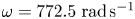$\omega =772.5\ \textrm {rad}\,\textrm {s}^{-1}$, meaning an excitation Strouhal number $St=\omega h/U_{Mean}=0.5$. The size of the vortex is $r_0=1\ \textrm {mm}$ in both cases. The exponential vortex is defined similarly. The missing two parameters are defined as $A_0=\varGamma /(2{\rm \pi} r_0^2)=1.591\ 1\,\textrm {s}^{-1}$ and $a_0=1$. The mesh dependence study was only done in the case of modified potential vortex formulation. The amplitude of the disturbance wave was $4.051\ \textrm {mm}\,\textrm {s}^{-1}$ in the case of coarse and $4.077\ \textrm {mm}\,\textrm {s}^{-1}$ in the case of fine grid. It means a difference of less than 1 %, which is acceptable. The amplitude of the disturbance wave along the centreline is displayed in figure 5 in both cases.

Figure 5.

The amplitude of the disturbance wave along the centreline of the jet in three different cases: modified potential vortex formulation and coarse grid; exponential vortex formulation and coarse grid; modified potential vortex and fine grid. The results cover each other in the case of modified potential vortex with different grid resolutions.

The result of the simulation for the modified potential vortex can be seen in figure 6. There a typical velocity field is plotted at $t = 0.4\ \textrm {s}$. The displacement of the jet is visible only far from the orifice, at the end of the domain, since the excitation is not very strong. The velocity components are monitored at 150 locations placed at the centreline of the jet. The transversal velocity signals are fast Fourier transformed using MATLAB 2017a. In each spectrum, a strong peak is obtained at the excitation frequency, as expected. This means that our model is able to excite the flow, and the jet responds with the same frequency as the excitation frequency.

Figure 6.

The velocity field of the simulation at $t = 0.4\ \textrm {s}$ in the case of the modified potential vortex.

The two vortex formulae were compared with each other with CFD simulations. The amplitude of the disturbance waves is plotted in figure 5.

The results show that the exponential vortex is very ineffective compared with the modified potential vortex. The transversal velocity amplitude of the generated disturbance wave is $0.003\ \textrm {m}\,\textrm {s}^{-1}$ at $x/h=15$, that is one order of magnitude smaller than that in the case of the modified potential vortex excitation. From this point, the modified potential vortex will be in the focus of the paper. Unless otherwise stated, all calculations will refer to that.

The full Navier–Stokes equations (CFD) simulation and the most unstable linear mode (at the excitation frequency) model are compared with each other. The Orr–Sommerfeld mode was calculated with the compound matrix method as described in Nagy & Paál (Reference Nagy and Paál2017). The $\alpha$ values were determined at every $x$ location for ${St}=0.5$. The response of the jet is modelled with Hill's method using the one mode with the highest growth rate. The strange mode found in our previous work (Nagy & Paál Reference Nagy and Paál2017) and experimentally (Zayko et al. Reference Zayko, Teplovodskii, Chicherina, Vedeneev and Reshmin2018) was excluded because it exists only near to the orifice. In the linear approach it has no effect downstream of the point of its disappearance. The real part of $\alpha$ (wavenumber) values was around 1.05–1.2, while their imaginary part (the opposite of the growth rate) was between $-0.7$ and $-0.12$. The amplitude of the mode ($C_0$) was calculated with the formula in (2.19). The integral was evaluated using the trapezoidal rule, where the grid was the same as in the CFD simulation. The amplitude of the transversal velocity fluctuations along the centreline is plotted in figure 7 for both cases. The nearly exponential growth of the disturbance wave can be seen in both cases. The difference between them is non-negligible, around 10 %. There are many reasons for this. First, the parallel-flow assumption is inaccurate close to the orifice. The more sophisticated methods of the parabolised stability equations (known as PSE) and its adjoint (known as APSE) could reduce this error (Dobrinsky & Collis Reference Dobrinsky and Collis2000). Furthermore, the amplitude of the disturbance wave is assumed to be zero at the orifice ($x/h=0$), while Blanc et al. (Reference Blanc, François, Fabre, de la Cuadra and Lagrée2014) showed that the excitation field has some effect already inside the nozzle. At the same time, the CFD simulation took around 10–12 h while the eigenvalues and modes can be determined in a few minutes. The direct and adjoint modes could be calculated in a reasonable time for a wide range of frequencies. Furthermore, the effect of acoustic excitation could be easily taken into account.

Figure 7.

The absolute value of the transversal velocity fluctuation (of the disturbance wave) along the centreline of the excited jet: continuous line, the CFD simulation; dashed line, the predicted value based on the technique developed by Hill (Reference Hill1995). OS stands for the Orr-Sommerfeld equation.

The last missing link to developing a new model of the edge tone is the prediction of the amplitude of excitation fields from the modes that will be discussed in the next section.

The velocity components of the adjoint mode were further investigated since they clearly show the most sensitive part of the disturbance waves (the locations where the wave can be excited more effectively). These fields are plotted in figures 8(a) and 8(b). It shows that the streamwise excitation can be effective along the two sides of the jet (two shear layers). (The flow enters into the domain at $x=0\ \textrm {mm}$ and between $y\in [-0.5, 0.5]\ \textrm {mm}$.) The strange thing is that the jet is less sensitive to transversal excitation compared with the streamwise one. At the same time, figure 8(b) shows that the transversal excitation is more effective close to the orifice than downstream. The importance of this is that the disturbance generated upstream will be amplified more than that generated downstream. The sensitivity to excitation in the upstream region is more relevant.

Figure 8.

The absolute value of the streamwise (a) and transversal (b) velocity component of the most unstable adjoint mode.

This effect is taken into account in figure 9(a) and 9(b), where the modes are multiplied by the exponential factor of (2.19). This clearly shows us that the flow is more sensitive very close to the orifice. The difference between the effectiveness of streamwise and transversal excitations is not so large as without the exponential factor. Similar results were found in our previous studies (Nagy & Paál Reference Nagy and Paál2016, Reference Nagy and Paál2017), where the growth rate was investigated and was found to be large close to the orifice.

Figure 9.

The absolute value of the streamwise (a) and transversal (b) velocity component of the most unstable adjoint mode multiplied by the exponential function of (2.19).

3.4. Incompressible dipole formulae

Our framework is able to handle any incompressible forcing field. Some models take into account the generated dipole at the edge in the feedback mechanism (Powell Reference Powell1961; Kwon Reference Kwon1998). An approximation of the compressible dipole for acoustically compact problems at low Mach numbers can be the incompressible, potential dipole. This dipole was also examined as a possible alternative for the vortex feedback model and as an agent of the excitation. The formulae of the velocity components of the modified potential dipole, so that the direction of the dipole is parallel with the $y$ axis, are

(3.11a)\begin{gather} u_{e, {dipole}} = \frac{2A_0 (x-x_0)\cdot(y-y_0) }{ ((x-x_0)^2+(y-y_0)^2+r_0^2 )^2 }, \end{gather}

(3.11b)\begin{gather}v_{e, {dipole}} ={-}\frac{A_0 ((x-x_0)^2 - (y-y_0)^2) }{ ((x-x_0)^2+(y-y_0)^2+r_0^2 )^2 }, \end{gather}

(3.11c)\begin{gather}w_{e, {dipole}} = 0, \end{gather}

where $A_0$ is the amplitude of the dipole and a parameter $r_0$, similar to the centre radius of the modified potential vortex, is also included to relax the singularity in the centre of the potential dipole.

4.1. Theory

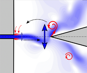
The schematics of the proposed feedback model is depicted in figure 10. Its main components are the convective disturbance amplification , the jet–edge interaction generating circulation , the circulation generating an excitation field and the excitation generating a disturbance wave . (In the case of the dipole and the exponential vortex feedback, the jet–edge interaction generates the excitation field. Components and are merged. The circulation does not play a role there. The amplitude is calculated in both cases from the velocity field at the edge, as discussed later.) Our model is constructed in Fourier space since the model is based on local linear stability theory of convectively unstable flows in which time-periodic disturbances are assumed. Because of this, the parts of the model will yield complex gains, which naturally incorporate the phase relation between the different processes.

Figure 10.

The schematics of the feedback loop model of the edge tone. The growth of the disturbance waves described by (2.17). The disturbance wave is ‘destroyed’ by the edge, which generates circulation. The circulation is calculated according to (4.5). The circulation generates an excitation velocity field (the vortex field) described by (3.8). The excitation velocity field generates a new disturbance wave, whose amplitude can be calculated with (2.19).

The edge-generated vortex field initiates instability waves. These waves travel downstream towards the edge and amplify due to the convective instability of the flow. This amplification is calculated with weakly non-parallel linear instability theory explained in § 2.2. This was realised by dividing the region between the nozzle and the edge into intervals, and at the left-hand end of each interval the stability equation was solved for several Strouhal numbers. The $n-1$ segments of the disturbance wave are defined as

(4.1)\begin{equation} \boldsymbol{u}_d=\sum_{i=1}^{n-1} \boldsymbol{u}_{i,d}, \end{equation}

where

(4.2)\begin{gather} \boldsymbol{u}_{i,d}=H(x-x_i)C_{0,i}\hat{\boldsymbol{u}}(y; x)\exp \left( \mathrm{i}\left(\int_{x_i}^{x}\alpha(\xi)\,\mathrm{d}\xi -\omega t\right)\right), \end{gather}

(4.3)\begin{gather} C_{0,i}= \int_{x_{i}}^{x_{i+1}}\int_{-\infty}^{\infty} \hat{\boldsymbol{s}}_{m, \hat{\varGamma}=1} \boldsymbol{\cdot} \hat{\boldsymbol{u}}^{{\dagger}}(y;\xi_1) \exp\left(\mathrm{i}\int_{0}^{\xi_1}-\alpha^{{\dagger}}(\xi_2)\,\mathrm{d}\xi_2\right) \,\mathrm{d}y\, \mathrm{d}\xi_1, \end{gather}

where $\hat {\boldsymbol {s}}_{m, \hat {\varGamma }=1}$ is the momentum source calculated with (3.7) using the vortex formula (3.8) for a unitary, periodic circulation ($\hat {\varGamma }_{in}=1$) and $H(x)$ is the Heaviside step function. The convective amplification (part of the feedback, see figure 10) of the instability waves originating in the $i$th interval (denoted by ${K_i}$) is independent of the amplitude of the original instability wave, and can be calculated only from the complex wavenumber,

(4.4)\begin{equation} {K_i}=\exp \left( \mathrm{i}\int_{x_i}^{x_{edge}}\alpha(\xi)\,\mathrm{d}\xi \right) . \end{equation}

The strength of the feedback (parts and , see figure 10) can be expressed with the amplitudes of the disturbance wave segments $C_{0,i}$. The disturbance wave arriving at the edge is considered to be the sum of all the disturbance waves emanating from each spatial interval and reaching the edge, so the total gain (defined later) is similarly the sum of all the gains for the subintervals. The disturbance wave at the edge induces a vortical field at the edge, which excites the jet upstream. This field is modelled as a modified potential vortex (see (3.8a)) located at the edge. One of the novelties is the estimation of the strength of the vortex field.

The effect of the edge is assumed to be such that it produces a vortex field with an opposite circulation compared with the incoming disturbance wave. The effect of the edge is assumed to be such that it tries to annihilate the incoming disturbance wave. The circulation and the core radius $r_0$ of the modified potential vortex was found by minimising the difference of the disturbance wave ($\boldsymbol {u}_d$) and the velocity field induced by the potential vortex ($\boldsymbol {u}_{e,{pot}}$) at the edge,

(4.5)\begin{equation} {\varGamma_{out}(t)}=\min_{\varGamma,r_0} \left( \int_{-\infty}^{\infty} \left| \boldsymbol{u}_{e,{pot}}(\varGamma,r_0) - \boldsymbol{u}_d \right|^{2} \,\mathrm{d}y \right)_{x=x_{edge}} , \end{equation}

which can be written in Fourier space in time

(4.6)\begin{equation} {\hat{\varGamma}_{out}(\omega)}=\min_{\hat{\varGamma},r_0} \left( \int_{-\infty}^{\infty} \left| \boldsymbol{\hat{u}}_{e,{pot}}(\hat{\varGamma},r_0) - \boldsymbol{\hat{u}}_d \right|^{2}\, \mathrm{d}y \right)_{x=x_{edge}}, \end{equation}

where

(4.7a,b)\begin{equation} \boldsymbol{u}_{e,{pot}}= \boldsymbol{\hat{u}}_{e,{pot}} \exp\left({-\mathrm{i}\omega t}\right) \quad \mathrm{and} \quad \boldsymbol{u}_d=\boldsymbol{\hat{u}}_d \exp\left({-\mathrm{i}\omega t}\right). \end{equation}

This calculation procedure can be easily applied to the exponential vortex or the incompressible dipole. There the amplitude ($A_0$) can be calculated instead of the circulation with a similar formula as (4.6).

The location of the vortex centre was also varied in the upstream and also the downstream direction from the tip of the edge. The method provided good results when the vortex was placed downstream of the edge, while it yielded erroneous results when the vortex was located upstream of the edge: the minimisation procedure found opposite circulations in these two cases. Therefore, we used another, more robust method for the estimation of the circulation. In this latter method, the circulation of the vortex field induced by the edge is assumed to be opposite to the circulation of the flow field upstream of the edge. This latter circulation is found by integrating along a contour which encloses the region upstream of the edge. Because in the far field ($y\to \pm \infty$), along the walls from which the jet issues and at the inlet the perturbation velocity is zero, the estimate for the circulation induced by the edge can be found by the following integral:

(4.8)\begin{equation} {\hat{\varGamma}_{out}(\omega) ={-}\left( \int_{-\infty}^{\infty} \hat{v}_{d}(x,y)\, \mathrm{d}y \right)_{x=x_{edge}}} \end{equation}

where $\hat {v}_{d}$ is defined as

(4.9)\begin{equation} v_d(x,y,t)=\hat{v}_{d}(x, y)\exp \left( -\mathrm{i}\omega t\right). \end{equation}

With the parameters of the modified potential vortex, the velocity field induced by it can be computed (part of the feedback). Here $\boldsymbol {\hat {u}}_d$ was calculated as the response field of the flow excited by a modified potential vortex ($\hat \varGamma _{in}=1$) of unitary circulation, and $\hat {\varGamma }_{out}$ expresses the open loop gain of the oscillation $G=\hat {\varGamma }_{out}/\hat {\varGamma }_{in}$. This expression can be calculated for all wave segments after substituting (4.1) and (4.3) into (4.5) and using that

(4.10)\begin{equation} {\hat{v}_{d}(x, y)=\hat{v}(y; x)\exp \left( \mathrm{i} \int_{0}^{x}\alpha(\xi)\,\mathrm{d}\xi\right),} \end{equation}

that finally leads

(4.11)\begin{equation} G(\omega)=\frac{\hat{\varGamma}_{out}}{\hat{\varGamma}_{in}}=\left(\sum_{i=1}^{n-1} C_{0,i} K_i\right) \hat{\varGamma}_{{eig}}. \end{equation}

Here, $\hat {\varGamma }_{{eig}}$ is the estimated circulation from the direct eigenvector and it can be calculated with the formula

(4.12)\begin{equation} \hat{\varGamma}_{{eig}}(\omega) =\min_{\hat{\varGamma},r_0} \left( \int_{-\infty}^{\infty} \left| \boldsymbol{\hat{u}}_{e,{pot}}(\hat{\varGamma},r_0) - \boldsymbol{\hat{u}} \right|^{2} \,\mathrm{d}y \right)_{x=x_{edge}} , \end{equation}

or with

(4.13)\begin{equation} {\hat{\varGamma}_{{eig}}(\omega)={-}\left( \int_{-\infty}^{\infty} \hat{v}(x,y) \,\mathrm{d}y \right)_{x=x_{edge}}} \end{equation}

and the local contribution of a wave segment can be defined as $G_i:=C_{0,i} K_i \hat {\varGamma }_{{eig}}$. This calculation will reveal the most important disturbance wave segments in the feedback mechanism.

An important parameter of these formulae is the vortex location. If the vortex centre is placed at the edge tip and the perturbation velocity is also evaluated there, in the minimisation procedure the transverse velocity component drops out (see (3.8b)). Since it was discussed before (4.8) that placing the vortex centre upstream of the edge tip leads to unphysical results, we placed the vortex centre downstream of the edge by $0.1$ non-dimensional units. The fact that the feedback originates downstream of the edge tip has been shown also by Kaykayoglu & Rockwell (Reference Kaykayoglu and Rockwell1986a) and Paál & Vaik (Reference Paál and Vaik2007). Our investigation showed that moving the vortex location farther downstream has only a small effect (moving the vortex by $1$ dimensionless unit downstream changed the frequency by less than $0.1\,\%$ using (4.13) and less than $1\,\%$ using (4.12)). In the case of the integral method (see (4.13)), the vortex core radius $r_0$ has to be prescribed. The effect of changing the core radius $r_0$ was also investigated. We found that in the interval $r_0\in [0.001, 3]$, the frequencies predicted by our model varied by less than $0.2\,\%$. Therefore the results presented in the following section were obtained by using $r_0=0.1$. As argued at the end of § 3.2 and also the good agreement with experiments indicate that the convection of the vortex from the edge tip does not play an important role in the feedback mechanism.

The two methods for estimating the circulation led to very similar results: the oscillation frequencies predicted by the models were the same (within 1 %) but the velocity difference minimisation usually estimated smaller open loop gains at most by a factor of $1/2$. The calculation of the model presented in this paper was obtained using the formula (4.13) because it proved to be more robust against sharp variations in the eigenfunctions in the case of the top-hat edge tone.

Similar investigations were carried out for the exponential vortex and the incompressible dipole forcing fields. In these cases, the amplitude ($A_0$) was estimated with a similar formula as (4.6) after substituting the proper velocity field. Since the exponential vortex is not singular, only the location of the centre was varied. It has minor effect on the frequency and significant influence on the gain. In the case of an incompressible dipole, the effect of $r_0$ and location of the the centre of the dipole were investigated. The parameter $r_0$ influenced the gain, but not significantly. Meanwhile, the location of the dipole has a remarkable effect on both the predicted frequencies and also on the gains. A good agreement of the frequencies was found with experiments if the dipole is placed farther than $0.3 h$ downstream of the edge tip.

The real part of the gain ($G$) expresses the amplification of the open loop, and with the imaginary part, the phase relationship can be determined. Since the amplification process repeats many times in the closed loop, the disturbance wave with the highest amplification will be favoured. The real part of the gain has several local maxima and they are very close to where the phase is zero (the real and the absolute value of gain is equal) and is usually cited as the phase criterion.

The feedback model takes into account the non-parallel nature of the flow, and also the variation of the phase speed and the growth rate of the disturbance waves, unlike previous models. The weakness of this model is its linearity, meaning that it has no nonlinear term which would limit the growth in the system. Therefore this model cannot predict the amplitude of the oscillations.

4.2. Validation of the complete feedback model

The feedback model is compared with the measurements of Vaik et al. (Reference Vaik, Varga and Paál2014a). The basis of comparison was the model with the modified potential vortex. The results are presented for this model unless otherwise stated. In their experimental configuration, the edge had a $30^\circ$ angle, and the nozzle–edge distance relative to the nozzle height was 9.72 in the case when the velocity profile at the nozzle exit was parabolic, and 10.26 when the exit velocity profile was top-hat. The nozzle–edge distance was divided into 200 intervals, and the investigated Strouhal number range ($St\in [0.008,{0.215}]$) was evaluated at 100 points.

Figure 11 displays the amplitude and phase curves of the loop gain at Reynolds number $Re=300$, in the case of the parabolic inlet velocity profile. For a nonlinear feedback loop, the condition $|G(St)|=1$ would correspond to the self-sustained oscillations. However, since this model is linear, it lacks nonlinear saturation; therefore, the gain can be significantly larger than unity. The gain curve as a function of $St$, after the initial increase, decreases monotonically. The phase curve is very similar to figure 16 in Holger et al. (Reference Holger, Wilson and Beavers1977), who deduced a phase criterion for the oscillation from their vortex model. Although the oscillation frequencies are identified as the local maxima of the real part of the gain, these Strouhal numbers are always close to the location of the zero phase, similarly to Holger et al. (Reference Holger, Wilson and Beavers1977).

Figure 11.

Gain absolute value and real part and phase plot from the feedback model as the function of the non-dimensional frequency. Parabolic inlet velocity profile, $Re = 300$.

Figure 12 displays the spatial variation of parts of the feedback loop as a function of the non-dimensional streamwise coordinate at $Re = 300$ and $St = 0.1145$, which corresponds to the maximum amplification. The convective amplification (${K}_i$) decreases exponentially because the disturbances triggered close to the nozzle have a larger distance to grow. The amplitude of the instability waves created by the forcing of the edge (${C}_{0,i}$) also decreases exponentially but it increases near the edge. The main reason for this is that although the velocity of the potential vortex scales with $1/D$ ($D$ is the distance upstream of the edge), the adjoint perturbation velocity, characterising the receptivity of the flow to external excitation, scales with $\exp (D)$, and the latter term dominates the product of the two quantities. The perturbations triggered close to the edge do not have a substantial contribution to the local gain ${G}_i$, since these instability waves do not have much room to grow. Consequently, the local gains (${G}_i$) also vary approximately exponentially. In the case of the top-hat velocity profile, the spatial variation of the above-mentioned quantities is qualitatively the same.

Figure 12.

Parts of the feedback loop as the function of the streamwise coordinate: ${K}_i$, downstream amplification; ${C}_{0,i}$, amplitude of the instability waves triggered by the forcing of the edge; ${G}_i$, local total gain. Parabolic inlet velocity profile, $St = 0.1145$, $Re = 300$.

The comparison between the predicted and measured oscillation frequencies for the parabolic inlet velocity profile are displayed in figure 13(a). The measured frequencies are represented with small black crosses, while the coloured circles represent the local maxima of the calculated amplification of the open loops. The colours show the logarithm with base 10 of the open-loop gain. The mode with the highest gain is connected with a continuous curve. Since the colours do not show unequivocally the strength of the modes, their open-loop gains were plotted in figure 13(b). At low Reynolds number, the model agrees well with the experiment. In both cases, mode 1 dominates, and the frequencies of the experiment and the model agree fairly well, although as the Reynolds number increases, the model tends to overpredict the oscillation frequency. Furthermore, the Reynolds number, where the frequency shift occurs, is also predicted well by our model. It occurred at Re = 180 in the experiment and $Re = 150$ in our model. Considering that in the 2-D CFD simulations of (Vaik et al. Reference Vaik, Paál, Kaltenbacher, Triebenbacher, Becker and Shevchenko2013) the first mode shift occurred at $Re = 150$, the prediction of the mode shift by the model is reasonable. The calculated frequency of the second stage (mode 2) agrees exceptionally well with the measurement. However, mode 1 and mode 3 coexist with mode 2 there. In the case of the first stage ($Re < 200$), at lower Reynolds numbers, the difference between the model and the measurement is not that significant, but the discrepancy takes substantial values as the frequency of the oscillation component drops at $Re\approx 200$. This is because, with the onset of the second stage, this frequency component is actually different from that of the first stage. In the second stage, this component is created by the nonlinear vortex–vortex interaction at the edge (Lucas & Rockwell Reference Lucas and Rockwell1984; Kaykayoglu & Rockwell Reference Kaykayoglu and Rockwell1986a), which cannot be captured by our linear model. In the experiments mode 2 disappeared at $Re\approx 650$, and the mode switching predicted by our model is also at $Re = 650$. The agreement between the model and the experiment in the prediction of the mode switching is remarkable. In the case of mode 2 and mode 3, the oscillation frequency predicted by the model also agrees exceptionally well with the experimental data. This suggests that at higher Reynolds numbers, the frequency selection is strongly dominated by linear amplification.

Figure 13.

(a) The comparison of the oscillation frequencies predicted by the model with the measurements of Vaik et al. (Reference Vaik, Varga and Paál2014a). The bluish circles indicate gains below one, i.e. no oscillation is generated there. (b) The absolute open loop gain of the calculated modes. Parabolic inlet velocity profile, nozzle–edge distance relative to the nozzle height is 9.72.

Figure 14 displays the oscillation frequency and the maximum amplification as functions of the Reynolds number with top-hat inlet velocity profile. The agreement with the experiments is similar to the previous comparison with the parabolic inlet velocity profile. Vaik et al. (Reference Vaik, Varga and Paál2014a) found that the first stage can be triggered by finite amplitude disturbances in the interval $Re\in [60,100]$: our calculations show that in this range the open loop gain of the first mode is close to unity, which indicates the onset of absolute instability. The model for mode 1 excellently predicts the oscillation frequency and the onset of the second stage is predicted with a better accuracy compared with the parabolic velocity profile. This occurs at $Re=200$ in our model and was observed at $Re\approx 200$ by Vaik et al. (Reference Vaik, Varga and Paál2014a). Considering that Brown (Reference Brown1937b) observed the mode switching at $Re=220$ for a wedge with an angle of $20^\circ$, the onset of mode 2 is predicted well by our model. In the experiments, with the appearance of mode 2, the frequency of mode 1 dropped similarly to the parabolic case, and following the previous discussion, the linear model is unable to predict the possibly nonlinear interaction. This approximately $25\,\%$ difference between simulations and experiments slightly increases at higher Reynolds numbers. With the arrival of mode 2, mode 3 could also be observed, although its amplitude was small. The predicted frequency differs by ${\approx }5\,\%$ for mode 2 but the discrepancy decreases as the Reynolds number increases. The frequency of mode 3 is predicted only crudely by the model. The less accurate prediction of higher modes is likely because in these modes since the wavenumber of the oscillations is small, a high degree of vortex roll-up occurs before the edge. This nonlinear effect is not considered in our model and, therefore, can cause this difference between simulation and measurement. In the first oscillation mode, this nonlinear vortex development is less significant; consequently, the frequency prediction is more accurate.

Figure 14.

(a) The comparison of the oscillation frequencies predicted by the model with the measurements of Vaik et al. (Reference Vaik, Varga and Paál2014a). The bluish circles indicate gains below one, i.e. no oscillation is generated there. (b) The absolute open loop gain of the calculated modes. Top-hat inlet velocity profile, nozzle–edge distance relative to the nozzle height is 10.26.

Finally, the modified potential vortex was replaced by the modified dipole and the exponential vortex. In the case of an exponential vortex, the frequency was in good agreement with the experiments. At the same time, the gain was extremely low. It was two orders of magnitude smaller than 1, which would be necessary for a sustained oscillation. This means that no oscillation can be sustained. In the case of an incompressible dipole, if the dipole is placed close to the edge, the predicted frequencies do not agree with experiments. If it is placed farther downstream ($L>0.3h$, $L$ is the distance from the edge tip) the frequencies are predicted accurately. At the same time, the gain was around one order of magnitude smaller than in the case of the modified potential vortex. For example, the gain of mode 1 is below 1 if $Re < 500$ in the case of parabolic profile and remains always below one in the case of top-hat profile ($r_0=0.1, L=0.5h$). The results are plotted here only for the parabolic profile in figure 15. This means that no oscillation can be sustained in a significant part of the investigated Reynolds number range, contradicting the experimental observations. If the dipole is placed farther downstream the gain increases. At the same time, this model still does not predict oscillation at Reynolds numbers below 200 for $L=1.1h$.

Figure 15.

The comparison of the oscillation frequencies predicted by the model with the measurements of Vaik et al. (Reference Vaik, Varga and Paál2014a). Modified incompressible dipole forcing field ($r_0=0.1$, $L=0.5h$), parabolic inlet velocity profile. The bluish circles indicate gains below one, i.e. no oscillation is generated there.