


1. Introduction
I welcome this opportunity to write a Perspectives article for JFM, and I thank the Editors for their invitation to do so. One dictionary definition of ‘perspective’ is ‘a particular attitude towards or way of regarding something; a point of view’. This gives me freedom to express my personal opinions throughout the article, and to adopt a more informal style than is perhaps usual for JFM.
Insofar as fluid dynamics is concerned with continuous deformation induced by flow, there is a natural symbiosis with topology which is largely concerned with properties of systems that remain invariant under continuous deformation. I propose to provide a necessarily superficial survey of a range of topics, all of which have some topological aspect, in which I have been personally involved at some stage over the last 60 years. Some of these topics involve flow at low Reynolds numbers, where viscous effects dominate; and some at high Reynolds numbers where viscous effects are negligible nearly everywhere. A particular concern in any topological approach is to identify the location and structure of singularities in a flow field, and the manner in which such singularities can be resolved (see § 3). A further concern is to identify flow properties that do indeed remain invariant, and to identify circumstances in which singularities can appear and topological jumps can occur; vortex reconnection is perhaps the best known circumstance of this kind, and my discussion will build up to a brief consideration of this problem and the implications for turbulence in § 11.
Magnetohydrodynamics plays an important part here in that, in an ideal conducting fluid, the magnetic field is ‘frozen in’, i.e. transported with the fluid (§ 5). Analogies with vortex dynamics and with steady Euler flows can be powerful in their implications, but must be treated with caution (§ 7). Topological properties are particularly relevant in both fast- and slow-dynamo theory (§ 6) and in the theory of magnetic relaxation (§ 8) which raises issues of stability (§ 9). This leads naturally to questions concerning the existence and structure of knotted flux tubes, and of field discontinuities that are inevitably encountered (§ 10).
My research in fluid dynamics started in 1958 under the supervision of George Batchelor FRS, whose centenary will be celebrated by a special IUTAM Symposium to be held in Cambridge, 15–18 March 2020.Footnote 1 In 1958, Batchelor was, at 38 years old, a world authority on turbulence, and he had founded this Journal just two years earlier (for details concerning this great achievement, see Moffatt (Reference Moffatt2017)). He was also at that time engaging with the authorities of Cambridge University in creating the Department of Applied Mathematics and Theoretical Physics (DAMTP), officially established in 1959. It was natural that I should undertake research in some aspect of turbulence, and I settled on Magnetohydrodynamic Turbulence (the title of my PhD thesis), magnetohydrodynamics being then at a very exciting stage of development following publication of the Interscience texts of Spitzer (Reference Spitzer1956) and Cowling (Reference Cowling1957). Batchelor was a superb research adviser, encouraging and critical at the same time, and unfailing in the good advice he gave at all stages of my early faltering attempts to grapple with ‘the problem of turbulence’.
I gladly dedicate this Perspective to George Batchelor, in memoriam.
2. Historical background
2.1. Helmholtz’ laws
My story starts with the seminal paper of Helmholtz (Reference Helmholtz1858), who stated his three laws of vortex motion for flow of an ‘ideal fluid’ in a bounded domain, laws which may be paraphrased as follows: (i) a vortex tube has constant circulation (i.e. flux of vorticity) along its length; (ii) a vortex tube must either be closed on itself or terminate on the fluid boundary; and (iii) vortex lines are transported with (or ‘frozen in’) the flow. This paper by Helmholtz was translated from German into English by Tait (Reference Tait1867), and came immediately to the attention of William Thomson (later Lord Kelvin) who recognised the particular significance of Helmholtz's law (iii), and immediately proposed his ‘vortex atom’ theory (Thomson Reference Thomson1867 – see below).
The first law (i) is merely a way of saying that  $\boldsymbol {\nabla }\boldsymbol {\cdot }\boldsymbol {\omega }=0$, which of course follows immediately from the definition of vorticity: $\boldsymbol {\omega }=\boldsymbol {\nabla }\wedge \boldsymbol {u}$, where ${\boldsymbol {u}}(\boldsymbol {x},t)$ is the velocity field. We shall use the symbol $\varGamma$ for the circulation of a vortex tube. The term ‘vortex filament’ may be used to describe a vortex tube of infinitesimal cross-section.
The statement of the second law (ii) is false, as now widely recognised, because in any flow that exhibits the (generic) phenomenon of chaos (see § 4 below), a vortex line in any chaotic sub-domain of the flow wanders indefinitely without ever closing on itself. Saffman (Reference Saffman1993) has maintained that the statement (ii) can be rescued by simply replacing ‘vortex lines’ by ‘vortex tubes’. In § 1.4 of his well-known book on Vortex Dynamics he wrote ‘If the vorticity field is compact, the tubes must be closed or begin and end on boundaries’. But this too is false; for in any chaotic sub-domain, any two neighbouring vortex lines diverge exponentially, and the cross-section of any vortex tube becomes increasingly flattened and distorted along its length; it will in general partially overlap itself, and does so repeatedly in these circumstances, but cannot surely be regarded as ‘closed’. (I made this point in my review of Saffman's book (Moffatt Reference Moffatt1994), and, following its publication, enjoyed an extensive correspondence with him about chaotic vector fields.)
2.2. Linked and knotted vortex tubes
The third law (iii) is most relevant to the theme of this Perspective, because it implies conservation of the topology of vortex lines, at least for so long as the velocity field remains ‘smooth’, i.e. at least  $\mathbb {C}^2$ (twice continuously differentiable). Linked vortex tubes remain linked, and knotted vortex tubes remain knotted. It was this property that in 1867 excited the attention of Kelvin, who two years later derived his famous ‘circulation theorem’ (Thomson Reference Thomson1869). James Clerk Maxwell was equally intrigued, as revealed by his correspondence with Tait; in a remarkable letter to Tait dated 13 November 1867 (reproduced from the original in figure 1a), Maxwell, with a degree of gentle scepticism, expresses his views concerning Thomson's ‘worbles’: he talks of ‘the interpretation Thomson has set himself to spin the chains of destiny out of a fluid plenum $\ldots$’ and adds ‘I saw you had put your calculus in it too. May you both prosper and disentangle your formulæ in proportion as you entangle your worbles’. (This was the beginning of an extended correspondence between Maxwell and Tait, who had been close friends ever since their schooldays at the Edinburgh Academy; Tait would frequently reply to Maxwell's letters by ha’penny postcards, whether to Cambridge or to Maxwell's estate in Glenlair, Dalbeattie (figure 1b), these postcards being densely packed on the other side with scientific comments and questions.) Amazingly, linked and knotted vortex tubes (Maxwell's ‘worbles’) have been realised experimentally only within the current decade (Kleckner & Irvine Reference Kleckner and Irvine2013). It is this fact, among others, that makes the topic of topological fluid dynamics (Moffatt & Tsinober Reference Moffatt and Tsinober1990) of such great current interest.
(a) First page of James Clerk Maxwell's letter to Peter Guthrie Tait, 13 November 1867; (b,c) Tait's frequent method of reply to Maxwell's letters. (Reproduced by kind permission of the Syndics of Cambridge University Library.)

2.3. Tait's classification of knots and the birth of topology
Tait's interest in vortex dynamics led him to initiate the classification of knots in a remarkable series of papers published during the 1870s, and now gathered together in his collected papers (Tait Reference Tait1898). These papers helped to open up the field of Topology as a distinct branch of mathematics. The word ‘topology’ made its first appearance in English in Tait's obituary of Johann Listing (Tait Reference Tait1883) who had introduced it in the German literature some decades earlier (Listing Reference Listing1848). As already remarked, topology and fluid mechanics have, or at least should have, a very natural symbiosis, in that both are concerned with continuous deformation, and with properties that in ideal circumstances remain invariant under such deformation. A marked divergence in theoretical developments in the century following Tait's seminal work – formal and rigorous in the case of topology, intuitive and exploratory in the case of fluid dynamics – led to a degree of schism between the two disciplines. Arnold's papers (Arnold Reference Arnold1965b, Reference Arnold1974) began a healing process, and the book of Arnold & Khesin (Reference Arnold and Khesin1998) has further highlighted the above symbiosis between the two fields.
2.4. Hicks vortex: a countable infinity of vortex knots
One further paper from the 1890s here deserves mention: Hicks (Reference Hicks1899) described what is now known as the ‘Hicks vortex’, an exact axisymmetric steady solution of the Euler equations, representing a family of vortex motions within a sphere. These vortices differ from the well-known ‘Hill's vortex’ in that they include a ‘swirl’ component of velocity around the axis of symmetry, so that the vortex lines lie on a family of nested tori within the sphere, and include a countable infinity of torus knots. The extent of the family of these torus knots, of interest from a topological point of view, has been recently clarified by Bogoyavlenskij (Reference Bogoyavlenskij2017) – see also Moffatt (Reference Moffatt1969).
3. Critical points and singularities
In topological fluid mechanics, the emphasis is on determining structural properties of a fluid flow. This generally starts with a need to locate critical points of the flow where the velocity or vorticity, or even some higher derivative, may be either zero or infinite; and then to analyse the structure of the flow in the neighbourhood of such points. As we shall see below, the streamline topology can change when zeros of velocity come into coincidence, and they can do so at infinite speed in a perfectly regular flow! We start by considering the relatively simple situation of two-dimensional incompressible flows. The situation when the velocity or vorticity may become infinite at a point is very much more difficult to analyse, and indeed it is not yet known whether such singularities can occur in incompressible flows of finite energy under Navier–Stokes, or even Euler, evolution. Consideration of this unsolved problem, necessarily speculative in character, is deferred to § 11 of this Perspective.
3.1. Two-dimensional flows
Consider an incompressible flow confined to a two-dimensional domain  $\mathcal {D}$ with boundary $\partial \mathcal {D}$. Such a flow is described by a streamfunction $\psi (x,y,t)$ and velocity components $u=\partial \psi /\partial y, v=-\partial \psi /\partial x.$ The instantaneous streamlines of the flow are given by curves $\psi = \textrm {const.}$, and must be distinguished from the particle paths, which are determined by the equations $\textrm {d}\kern0,05em x/\textrm {d}t=u(x,y,t), \textrm {d}y/\textrm {d}t=v(x,y,t)$, and initial conditions $\boldsymbol {x}(0)=\boldsymbol {a}$, say. If the flow is steady (i.e. $\partial \psi /\partial t =0$), then the particle paths coincide with the streamlines.
At ‘stagnation points’ where the fluid is instantaneously at rest,  $\partial \psi /\partial x=\partial \psi /\partial y=0$; these are ‘critical points’ of $\psi$, extrema (maxima or minima) if the local streamlines are elliptic, saddle points if they are hyperbolic. If $\mathcal {D}$ has the topology of a disc, and if the critical points of $\psi$ are all in the interior of $\mathcal {D}$, then the number of extrema $n_{e}$ and the number of saddle points $n_{s}$ are related by Euler's identity $n_{e} - n_{s}=1$. This is the simplest result of a topological character for such a flow, and it holds at all times during the evolution of the flow. If, for example a saddle point merges with an extremum, then both $n_{e}$ and
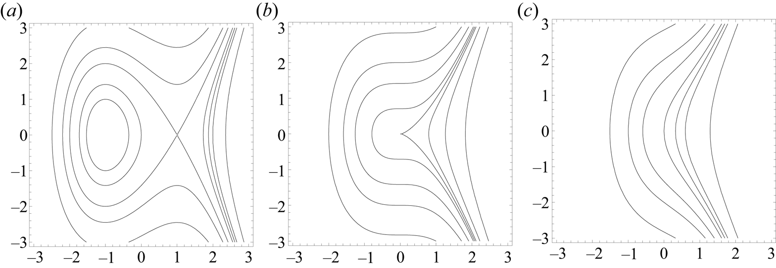
  $n_{s}$ decrease by one, and the difference is conserved. The situation is illustrated in figure 2 by the streamfunction $\psi =\psi _1 = y^2-x^3 -3xt$; here, $u=2y, v=3x^2+3t$ and for $t<0$, there are stagnation points at $x=-\sqrt {-t}$ (an extremum) and at $x=+\sqrt {-t}$ (a saddle). The separation of these points decreases at speed ${\sim }(-t)^{-1/2}$, and they merge (at infinite speed!) at $t=0$. Note the cusped structure of the critical streamline $\psi _1=0$ at $t=0$. This is an instantaneous topological transition, of a type that regularly occurs in the evolution of meteorological maps. We note further that $\psi _1$ trivially satisfies the unsteady non-dimensionalised Stokes equation $\partial \nabla ^2\psi _1/\partial t = \nabla ^4 \psi _1$, so that, since the nonlinear inertia force is negligible near the stagnation points, this transition is dynamically realisable under Navier–Stokes evolution.
Figure illustrating the merging of two stagnation points (an extremum and a saddle) as  $t$ increases through zero for the streamfunction $\psi (x,y,t)=y^2-x^3 -3xt$; (a) $t=-1$, (b) $t=0$, (c) $t=+1$; the cusped streamline exists only instantaneously at time $t=0$.
It may happen that a critical point lies on the boundary  $\partial \mathcal {D}$ of the domain. In this case, a streamline $\psi = \textrm {const.}$ intersects the boundary at the critical point. This is illustrated in figure 3 for the streamfunction $\psi =\psi _{2}= y^2(y-kx)$, for which $u=3y^2-2kxy, v=ky^2$. Since $\nabla ^{4}\psi _{2}=0$, this represents a Stokes flow with no slip on the boundary $y=0$, and what may (for $k>0$) be described as ‘Stokes separation’ at $x=0, y=0$ (or ‘Stokes reattachment’ if $k<0$). Each such boundary structure is like ‘half of a saddle point’ and contributes $1/2$ to $n_{s}$ in Euler's identity.
Stokes flow described by the streamfunction  $\psi = y^2(y-kx)$, with no slip on the boundary $y=0$.

3.2. Corner flow and Stokes separation
Consider first the classic problem of two-dimensional flow in a corner between two planes  $\theta ={\pm }\alpha$. It is supposed that the flow is driven by some unspecified mechanism (e.g. a rotating cylinder) far from the corner, and it is required to analyse the asymptotic behaviour near the corner. I was attracted to this problem in 1962 when required to set examination questions on a Masters’ level course on viscous flow theory; the fruitful interaction between teaching and research was never more evident! The natural approach, as had been suggested by Rayleigh (Reference Rayleigh1920, p. 18) and pursued by Dean & Montagnon (Reference Dean and Montagnon1949), was to assume a streamfunction of the form
 \begin{equation} \psi(r,\theta)=r^{\lambda}f(\theta), \end{equation}
in plane polar coordinates, to substitute this in the biharmonic equation  $\nabla ^4 \psi =0$ governing the Stokes flow near the corner, and then to seek to determine $\lambda$ by satisfying the no-slip conditions on the bounding planes. If it is supposed that $\psi$ is symmetric approximately $\theta =0$, this leads to the equation
 \begin{equation} \sin{2\mu\alpha}={-}\mu\sin{2\alpha}\quad \text{where}\ \mu=\lambda-1. \end{equation}
The novel property of this equation is that all non-zero solutions for  $\mu$ are complex if $2\alpha \lesssim 146.3^{\circ }$. This much had been discovered by Dean & Montagnon (Reference Dean and Montagnon1949), but the fact that this implies infinite oscillations as $r\rightarrow 0$ was not recognised by these authors. I found it difficult to believe this myself, and I took the prediction to George Batchelor, expecting him to say there must be a mistake somewhere. To my great relief, he said ‘Yes, I can believe that’, and gave me every encouragement to write my paper on this topic (Moffatt Reference Moffatt1964); he obviously approved of my efforts to extract physical meaning from such a curious mathematical result! The function $f(\theta )$ in (3.1) is also complex, but since the Stokes problem is linear, we may simply redefine $\psi$ as $\textrm {Re}\,[r^\lambda f(\theta )]$. The resulting streamfunction exhibits a geometric sequence of counter-rotating eddies, as illustrated for the case $\alpha ={\rm \pi} /18$ in figure 4(a). The important thing about this flow is that it exhibits the phenomenon of flow separation and reattachment where the dividing streamlines $\psi =0$ meet the boundaries $\theta ={\pm }\alpha$. Near these points, the flow is just as described in figure 3, with $k>0$ for separation and $k<0$ for reattachment. Separation had previously been thought of as a high-Reynolds-number phenomenon; but here it was also evident, and quite dramatically so, at low Reynolds number also. $(a)$ Eddies in a corner of half-angle $\alpha ={\rm \pi} /18$ described by the streamfunction $\psi =r^{\lambda }f(\theta )$, where $\lambda$ is determined by (3.2); $(b)$ corner eddies. (from Taneda Reference Taneda1979, with permission)

The flow shown in figure 4(a) was realised experimentally by Taneda (Reference Taneda1979), who observed the first two eddies in a sequence driven by rotation of a cylinder far from the corner (figure 4b). A third eddy could also be dimly discerned, although the velocity in it was extremely small. The theory does indeed imply a rapid decrease in flow intensity from one eddy to the next as the corner is approached – by a factor of approximately 400 when  $\alpha ={\rm \pi} /18$. If the first eddy has a circulation time of say 10 s, then the second will have a circulation time ${\sim }1\ \textrm {h}$, the third ${\sim }16$ days, and the fourth ${\sim }17$ years; to observe such eddies demands patience! Indeed, the fluid is virtually stagnant after the third eddy in the sequence, whatever the remote stirring mechanism may be; and yet, because $\lambda$ is not an integer, high derivatives of the velocity are infinite at $r=0$ for nearly all values of the angle $\alpha$!
3.2.1. The competition between forced and free solutions
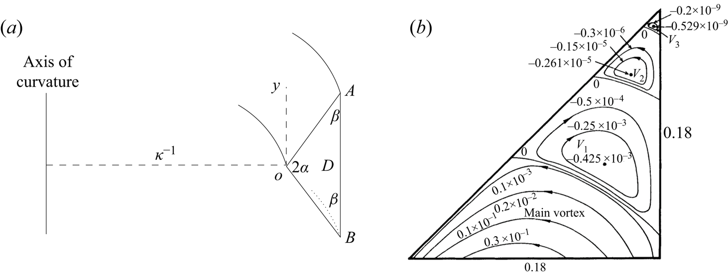
Corner eddies are present in a very wide variety of flows, and have gained some prominence through the current importance of micro- and nano-hydrodynamics (Squires & Quake Reference Squires and Quake2005), where the Reynolds number is undoubtedly small enough for application of the theory. An instructive example is provided by the pressure-driven flow in a curved triangular duct studied numerically by Collins & Dennis (Reference Collins and Dennis1976). The geometry is shown in figure 5(a): the triangular duct is supposed curved about the vertical axis, with radius of curvature  $L$ large compared with the scale of the duct cross-section. The resulting centrifugal force drives a secondary flow, which exhibits the corner eddies shown in figure 5(b).
The curved duct configuration of Collins & Dennis (Reference Collins and Dennis1976). When the flow is pressure driven, eddies form at A and B if  $\beta > 40.4^{\circ }$, and at O if $71.9^{\circ } < 2\alpha < 159.1^{\circ }$. When the flow is driven by rotation of the boundary AB about the axis of curvature, eddies do not form at A and B, but they do form at O if $35.0^{\circ } < 2\alpha < 159.1^{\circ }$ (after Collins & Dennis Reference Collins and Dennis1976).
The question of whether eddies do or do not form in such circumstances is determined by the dependence of the driving force on the distance  $r$ from the corner. The pressure-driven velocity $w$ is $O(r^2)$ near the point A, and the streamfunction $\psi$ of the secondary flow is determined by
 \begin{equation} \nu \nabla^4 \psi ={-}2\kappa w \,\partial w/\partial y \quad \text{in}\ \mathcal{D};\quad w =\partial w/\partial n=0 \quad \text{on}\ \mathcal{\partial D}. \end{equation}
Since  $w \partial w/\partial y\sim r^3$, it follows that the particular integral of (3.3a,b) as $r\rightarrow 0$ is $O(r^7)$. Eddies will form if, for the angle $\beta$ (here ${\rm \pi} /4$), $\textrm {Re}\,\lambda <7$, for then the (homogeneous) complementary function dominates as $r\rightarrow 0$. The dependence of $\lambda$ on $\beta$ being known, this condition translates to $\beta \gtrsim 40.4^{\circ }$, so that eddies do indeed form when $\beta ={\rm \pi} /4$. Collins & Dennis (Reference Collins and Dennis1976) computed the geometric sequence of these eddies by successive grid refinement as the corner is approached. Similar arguments determine whether eddies will form at the corner $O$, where the secondary flow is symmetric about the bisector. So far as I am aware, these predictions have not yet been subjected to experimental verification; it would be sufficient to bend the axis of such a duct gently through an angle, to drive flow through the duct by an applied pressure gradient, and to visualise the cross-sectional flow by a transverse sheet of light at the bend.
3.3. Universality
The beauty of the corner flow solution  $\psi \sim \textrm {Re} \, r^{\lambda }f(\theta )$ lies in what may be described as the ‘universality’ of the phenomenon that it describes. First, although this appears to be a low-Reynolds-number phenomenon, this form of $\psi$ actually provides an asymptotic solution of the Navier–Stokes equations for arbitrary ‘driving Reynolds number’ $Re$ (i.e. based on the driving mechanism far from the corner). This is because both the local length scale and the flow velocity tend to zero as $r\rightarrow 0$. Thus the Stokes separation phenomenon is universal for arbitrary $Re$ and arbitrary two-dimensional flow near a corner, provided that the angle of the corner is $\lesssim 146.3^{\circ }$. The location of the first separation point depends on the remote forcing mechanism; moreover, this location will be Reynolds-number dependent in a manner that still calls for detailed investigation.
Second, even if the corner is not sharp (and no corner is perfectly sharp in reality), the flow will still in general in the low- $Re$ regime exhibit a sequence of counter-rotating eddies, but the number of these will be finite; indeed if flow is driven by a rotating cylinder placed in a converging channel, it may be expected to exhibit a similar eddy sequence. If there is a weak superposed flow through the channel, then the eddies are attached alternately to the walls of the channel, allowing the flow to pass between them.
A similar phenomenon occurs at a cusped corner, e.g. in steady shear flow over a cylinder that sits on a plane boundary: the flow separates and a sequence of eddies appears in the cusp regions, both upstream and downstream because (at low  $Re$) the flow exhibits symmetry about the diameter of the cylinder through its point of contact with the plane. If there is a small gap between the cylinder and the plane, then there is a small leakage of fluid through the gap, and the eddies, again finite in number, are in this case attached alternately to the cylinder and the plane (Jeffrey & Sherwood Reference Jeffrey and Sherwood1980).
3.4. Free-surface singularities
A very different type of singularity can occur at the free surface of a liquid of viscosity  $\mu$ and surface tension $\gamma$ when some sub-surface forcing causes convergence of the flow at the free surface, as shown in figure 6(a). Here two cylinders of equal circular cross-sections, placed at the same level below a free surface, are counter-rotated to generate a converging flow at the free surface; at sufficient speed of rotation the surface is drawn down on the plane of symmetry and a cusp-type singularity is observed to form. Figure 6(b) shows an idealisation of this situation, in which the rotating cylinders are replaced by a vortex dipole of strength $\alpha$ at depth $d$ below the surface, thus inducing the same type of converging flow at the surface. The gain here is that this problem can be solved exactly assuming Stokes flow and neglecting the influence of gravity, a neglect that may be justified retrospectively (Jeong & Moffatt Reference Jeong and Moffatt1992). $(a)$ A cusp at the free surface of a viscous liquid induced by sub-surface counter-rotating cylinders (the cylinder on the left rotates clockwise, that on the right anti-clockwise); the black streak entering the fluid from the cusp marks a thin sheet of air that enters the bell-shaped bubble which is held stationary in the downward flow; $(b)$ flow modelled by a vortex dipole of strength $\alpha$ at depth $d$ below the position of the free surface when undisturbed; the cusp appears at depth $2d/3$; $(c)$ local situation near the stagnation point on the plane of symmetry (adapted from Jeong & Moffatt Reference Jeong and Moffatt1992).

Formation of the cusp involves a battle between viscosity and surface tension. The following simple argument (provided by J. Hinch, private communication) indicates why the apparent cusp forms despite the smoothing effect that is usually associated with surface tension. Flow near the stagnation point on the plane of symmetry (figure 6c) is in part due to a (virtual) point force  $2\gamma$ upwards located roughly at the centre of curvature of the free surface, and in part to a downward velocity $U$ due to the remote forcing. The upward velocity due to the point force is essentially that of a Stokeslet: $u=(\gamma /2{\rm \pi} \mu )\log {r_0/r}$ for some $r_0$, and this balances $U$ at $r=R$ (the radius of curvature at the ‘cusp’) where $R/r_0=\exp {[-2{\rm \pi} \mu U/\gamma ]}$. For the model problem of figure 6(b), on dimensional grounds $r_0=c_{1} d,\, U=c_{2}\alpha /d^2$ where $c_1$ and $c_2$ are dimensionless constants, so that
 \begin{equation} R/d = c_{1}\exp{[{-}2{\rm \pi} c_{2}C]}, \end{equation}
where  $C=\mu \alpha /\gamma d^2$, the capillary number.
This argument shows the power of dimensional argument combined with physical intuition; determination of the constants  $c_{1}$ and $c_{2}$, however, requires the full analytical solution of the problem, which yields $c_{1}=256/3, c_{2}=16$. Now, if we assume a ‘level playing field’ as between viscosity and surface tension (i.e. $C=1)$ then (3.4) gives the extraordinary result
 \begin{equation} R/d \approx 1.9 \times 10^{{-}42} \quad \text{or equivalently} \quad d/R \approx 5.3\times 10^{41}. \end{equation}
 From a mathematical point of view, it is remarkable that such numbers should emerge from a problem whose statement as a nonlinear boundary-value problem itself involves no small parameters. Here, allow me to draw attention to Richard Feynman's thought-provoking discussion (Feynman, Leighton & Sands Reference Feynman, Leighton and Sands1963) concerning the extremely large ratio of the electrical repulsion of two electrons to their gravitational attraction,  $4.17\times 10^{42}$. Feynman writes: ‘Where could such a tremendous number come from? Some say that we shall one day find the “universal equation”, and in it, one of the roots will be this number. It is very difficult to find an equation for which such a fantastic number is a natural root’. Well, I don't of course wish to suggest that cusp singularities have any implications for a unified field theory; but merely to point out that huge numbers (or their reciprocals) can indeed emerge from certain nonlinear boundary-value problems arising in very classical fluid-dynamical contexts.
3.4.1. High-Reynolds-number cusping, and air entrainment
Again, I would claim that the result (3.4) has a universality that transcends the particularity of the vortex-dipole prescription. The same cusping phenomenon is to be expected even if the Reynolds number based on the remote forcing is large; this is because as for the corner flow problem, irrespective of this ‘global’ Reynolds number, inertia forces are negligible near the stagnation point where the cusp forms. A good example of the high-Reynolds-number situation is provided by the problem of the impact of a steady stream of water from a tap onto a deep tank of water, an experiment that is easily performed at bath time! When the downward flux is small, the flow is quite steady; but as the flow rate is increased, a critical stage is reached at which bubbles appear in the bath near the region of impact, with audible effect. The reason is that a circular cusp forms where the stream impacts the free surface, and air is entrained into the bath through the cusp by the mechanism described by Eggers (Reference Eggers2001). This mechanism, which resolves the cusp singularity, is presumably fundamental whenever air is mixed into water, as through breaking waves, or indeed whenever any two immiscible fluids are vigorously stirred together to enhance interaction, a frequent objective in chemical-engineering processes. The process of air entrainment has been studied in computational detail by Kumar, Das & Mitra (Reference Kumar, Das and Mitra2017), who also provide an extensive list of the many contributions to this problem since 1990.
Air entrainment through the cusp is indicated by the black streak descending from the cusp in figure 6; this air enters the bell-shaped bubble (black), which remains stationary in the downward flow shedding much smaller bubbles into the stream. This phenomenon can be seen quite clearly if the cylinders of figure 6(a) are brought into close proximity, as in figure 7. Here again, air is drawn through the cusp in a thin sheet emerging into a bell-shaped bubble, with again ‘detrainment’ of small air bubbles from the two lower cusps. An investigation of this configuration by lubrication theory could be illuminating.
As in figure 6, but here the cylinders are close to each other, and only partially submerged; (a) the viscous fluid is drawn up in a layer on each cylinder and the layers interact as the fluid passes down through the gap, forming a cusp; the free surface can be seen on the right of the photo; (b) blow-up of the cusp region showing how air is drawn through the cusp in a very thin sheet forming a ‘tricuspidal’ bubble from which smaller bubbles of air are ejected into the fluid. (Photographs taken by author in 1992, but not previously published.)

The exact solution that leads to the result (3.4) also gives the velocity field; at distance  $r$ from the cusp just outside the parabolic region shown in figure 6(c), the downward velocity component has the asymptotic form $v \sim -U +O(r^{1/2})$, so that the local rate of strain is $O(r^{-1/2})$ (a singularity that is resolved as indicated above by air entrainment). The associated rate of dissipation of energy is $O(r^{-1})$ so area integrable at $r=0$. Care is of course needed in the double limiting process $C\rightarrow \infty , r\rightarrow 0$.
3.4.2. The Herculean paradox
A related situation is provided by the problem of a vertical flat plate pushed with velocity  $U$ through the free surface of a viscous fluid. On the (untenable) assumption that the free surface remains horizontal (figure 8a), the local streamfunction would have the form $\psi \sim U r f(\theta )$, as in the Taylor ‘paint-scraper’ problem (Taylor Reference Taylor1960). This would lead to a non-integrable stress ${\sim }r^{-1}$ on the plate, so that the force needed to impel it downwards would be infinite; hence the frequently quoted ‘Herculean paradox’ that not even Hercules could (as alleged in Greek mythology) have dipped his arrows in the envenomed blood of the Hydra without truly superhuman strength. $(a)$ Hypothetical (but unrealistic) flow near the contact line when a flat plate is drawn into a viscous fluid with velocity $U$;
$U$;  $(b)$ the ‘half-cusp’ between the free surface and the plate that must occur near the contact line due to the downward drag on the fluid.
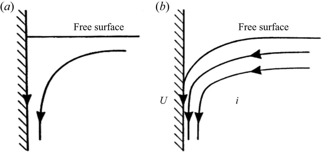
However, the fluid is in fact drawn down by the viscous force as indicated in figure 8(b), and the flow in the immediate neighbourhood of the contact line actually looks very similar to the cusp flow if we simply place a vertical plate on the plane of symmetry of that flow and move it downwards with the velocity  $U$ at the cusp as obtained from the exact cusp solution. All the conditions of the problem are then satisfied: the flow satisfies the biharmonic equation, and the required conditions on the free surface and on the vertical plate are locally satisfied. The cusp solution (Jeong & Moffatt Reference Jeong and Moffatt1992) gives a local stress of order $r^{-1/2}$, and so integrable on the plate. The force required to impel it downwards is therefore finite (and actually independent of capillary number provided this is of order unity or greater). We may thus dispose of the Herculean paradox.
4. Lagrangian chaos
4.1. ABC flow
The flows considered so far have been regular in the sense that the streamlines and/or particle paths are either closed curves or curves confined to a family of surfaces. The generic structure of steady flows in three dimensions does not satisfy either of these constraints; in general, there exist subdomains within the fluid in which the streamlines are space filling: they wander in such a way as to come arbitrarily near any point of the subdomain if followed far enough. Such flows exhibit what is described as ‘Lagrangian chaos’. The behaviour occurs also in unsteady two-dimensional flows, as exemplified by the ‘blinking vortex’ model of Aref (Reference Aref1984).
Chaos in fluid flows was a subject that sprang to life with the work of Arnold (Reference Arnold1965a) and Hénon (Reference Hénon1966), who studied what came to be known as the ABC flow,
 \begin{equation} {\boldsymbol{u}}(\boldsymbol{x})= (B \cos ky +C \sin kz, C\cos kz + A\sin kx, A\cos kx +B\sin ky), \end{equation}
which satisfies the Beltrami condition  $\boldsymbol {\omega }(\boldsymbol {x})=k{\boldsymbol {u}}(\boldsymbol {x})$. Any incompressible flow ${\boldsymbol {u}}_B$ satisfying this condition (with $k$ constant) also satisfies the condition $\nabla ^2 {\boldsymbol {u}}_B \equiv -\boldsymbol {\nabla }\times \boldsymbol {\omega }_B = -k^2 {\boldsymbol {u}}_B$, and therefore satisfies the Navier–Stokes equation (linear for such flows),
 \begin{equation} \partial {\boldsymbol{u}}_B/\partial t ={-}\boldsymbol{\nabla} \varPi -k^2 {\boldsymbol{u}}_B, \end{equation}
where  $\varPi =p/\rho +{\boldsymbol {u}}_B^2/2$. With $\varPi = \textrm {const.}$, this has the exponentially decaying solution ${\boldsymbol {u}}_B(\boldsymbol {x},t)={\boldsymbol {u}}_B(\boldsymbol {x},0){\text {e}}^{-k^2 t}$, a result recognised in an early paper by Trkal (Reference Trkal1919) (available in English translation since 1994). Thus the streamline structure remains constant under Navier–Stokes evolution in this very special situation.
The flow (4.1), being periodic in  $x,y$ and $z$, can be treated as a flow on the three-torus $\mathbb {T}^3$, a description that may be less than helpful for those who prefer to remain firmly in the Euclidean space $\mathbb {R}^3$, in which the flow can actually occur. Nevertheless, it is on $\mathbb {T}\,^3$ that the streamlines of the flow are chaotic. This chaos has been studied in some detail by Dombre et al. (Reference Dombre, Frisch, Greene, Hénon, Mehr and Soward1986) who summarise their results with the statement ‘In general, there is a set of closed (on the torus $\mathbb {T}^3)$ helical streamlines, each of which is surrounded by a finite region of Kolmogorov–Arnold–Moser invariant surfaces. For certain values of the parameters strong resonances occur which disrupt the surfaces. The remaining space is occupied by chaotic particle paths: here stagnation points may occur and, when they do, they are connected by a web of heteroclinic streamlines’. A typical Poincaré section is reproduced in figure 9(a) for the particular case $A^{2} =1, B^{2} =2/3, C^{2} =1/3$, showing ‘islands of regularity’ within a sea of chaos which extends over roughly half the fluid domain; a single streamline here provides the scatter of points in the chaotic region. Generally, it appears that the region of chaos decreases in extent as the parameters $A, B$ and $C$ approach equality, although a modest extent of chaos survives in the limiting situation, as shown in figure 9(b).
Sample Poincaré sections for the ABC flow;  $(a)$
$(a)$  $A^{2} =1, B^{2} =2/3, C^{2} =1/3$, showing islands of regularity in a sea of chaos; $(b)$ the contrasting situation when $A^{2} =1, B^{2} =1, C^{2} =1$; the region of chaos is very much reduced. (From Hénon Reference Hénon1966; Dombre et al. Reference Dombre, Frisch, Greene, Hénon, Mehr and Soward1986.)

4.2. Stokes flow with chaos
Stokes flows, for which inertia effects are completely negligible, have found an important field of application in microfluidic systems whose scale is such that  $Re \ll 1$ (Squires & Quake Reference Squires and Quake2005). A different type of Lagrangian chaos can exist in such systems. Figure 10(a) shows a typical streamline for a steady Stokes flow in a sphere, and figure 10(b) an associated Poincaré section for the same streamline when it is continued for a very long time. In figure 10(a), the streamline appears to lie on a surface; but the Poincaré section shows that this is not in fact the case: the ‘surface’ shifts by random small amounts when it nearly returns on itself – a phenomenon described as ‘transadiabatic drift’ (Bajer & Moffatt Reference Bajer and Moffatt1990). $(a)$ Typical streamline of a flow of the form ((4.3), (4.4a–c)) which indicates two strong vortices; $(b)$ Poincaré section for the same streamline by a plane perpendicular to the vortices, showing points where it has crossed the plane of section 40 000 times. (From Bajer & Moffatt Reference Bajer and Moffatt1990.)

The particular Stokes flow with streamlines as in figure 10 is one of a class of steady flows consisting of three ingredients, each of which is an incompressible Stokes flow confined to the sphere  $r<1$
$r<1$
 \begin{equation} {\boldsymbol{u}}(\boldsymbol{x}) =\boldsymbol{U}(\boldsymbol{x}) +\boldsymbol{V}(\boldsymbol{x}) +\boldsymbol{W}(\boldsymbol{x}), \end{equation}
where
 \begin{align} \boldsymbol{U}(\boldsymbol{x})=\boldsymbol{a}(1-2r^2) +(\boldsymbol{a}\boldsymbol{\cdot} \boldsymbol{x})\boldsymbol{x},\quad \boldsymbol{V}(\boldsymbol{x})={\boldsymbol{\varOmega}}\times\boldsymbol{x},\quad \boldsymbol{W}(\boldsymbol{x})=(\lambda yz,\mu zx,\nu xy), \end{align}
and where  $\lambda +\mu +\nu =0$ (so that $\boldsymbol {W}\boldsymbol {\cdot } \boldsymbol {n}=0$ on $r=1$). Here, $\boldsymbol {U}(\boldsymbol {x})$ is the same as the flow inside a Hill's spherical vortex, axisymmetric about the vector $\boldsymbol {a}$, $\boldsymbol {V}(\boldsymbol {x})$ is a rigid body rotation with angular velocity $\boldsymbol {\varOmega }$ and $\boldsymbol {W}(\boldsymbol {x})$ is a combination of ‘twist ingredients’; this type of flow was originally devised to represent the ‘stretch–twist–fold’ process, believed to be fundamental for dynamo theory (see § 6.3 below). Each such flow ${\boldsymbol {u}}(\boldsymbol {x})$ inside the sphere $r=1$ has to be driven by a non-zero tangential velocity on the surface $r=1$ and the associated tangential stress; thus energy is pumped into the sphere from the surface and dissipated internally by viscosity. If the amplitude of the flow is normalised (e.g. by setting $\lambda ^2 +\mu ^2 +\nu ^2=1$), there remains a seven-parameter family of flows of this kind, all quadratic functions of the space coordinates, all Stokes flows in a sphere, and all exhibiting some degree of chaos except in limiting situations, as described in Bajer & Moffatt (Reference Bajer and Moffatt1990). The flow shown in figure 10 looks as if the streamline lies on a surface around two vortices; but in fact when this streamline (or equivalently particle path) is continued for a long time, the Poincaré section by a plane perpendicular to the vortices shows a high degree of chaos in the flow.
A similar situation arises when a small drop, kept spherical by surface tension, is subjected to a general strain field in the surrounding fluid (Stone, Nadim & Strogatz Reference Stone, Nadim and Strogatz1991). The Stokes flow inside the drop in this situation is a cubic function of the cartesian coordinates, and again the particle paths in general exhibit Lagrangian chaos. An important, indeed defining, property of this type of Lagrangian chaos is that initially neighbouring particle paths diverge exponentially when averaged over a long time (i.e. the Lyapunov exponent is positive), at least until the separation is comparable with the scale of the drop. A small blob of dye in such a flow is stretched into a thin highly convoluted sheet as time progresses. The behaviour is conducive to strong mixing, important when homogeneity within the droplet is the objective.
5. Frozen-in fields
The topological aspect of fluid mechanics is most prominent in consideration of properties, whether scalar or vector or even higher-order tensor, that are transported with the flow. For example if a dye is used to colour a subdomain  $\mathcal {D}_L$ of the fluid, and if molecular diffusion is neglected, then this coloured region is obviously transported with the flow, i.e. $\mathcal {D}_L$ is a Lagrangian subdomain. We say that the dye is ‘frozen in the fluid’, or simply that it is a ‘frozen-in’ field. As recognised by Helmholtz, vorticity in an ideal fluid is a frozen-in vector field, the vortex lines being transported with the flow and the circulation round any material (Lagrangian) circuit being conserved. These are the two most familiar examples of frozen-in fields, which we now consider in more detail.
5.1. Frozen-in scalar fields
If a passive scalar ‘dye’ is injected into an incompressible flow field, it is in general convected and diffused according to the equation
 \begin{equation} \textrm{D}\theta/\textrm{D}t\equiv \partial\theta/\partial t +{\boldsymbol{u}}\boldsymbol{\cdot}\boldsymbol{\nabla} \theta =\kappa \nabla^2\theta, \end{equation}
where  $\theta (\boldsymbol {x}, t)$ is the dye-concentration field, and $\kappa$ its molecular diffusivity relative to the fluid. The relative importance of convection as compared with diffusion is quantified by the Péclet number $Pe=UL/\kappa$, where $U$ and $L$ are scales of velocity and length associated with the distortion of the dye field.
If molecular diffusion is negligible to the extent that we may assume  ${\textrm {D}}\theta /{\textrm {D}}t =0$, then the surfaces $\theta = \textrm {const.}$ are transported with the flow $\boldsymbol {u}$, i.e. these surfaces are ‘frozen in the fluid’. For a localised ‘blob’ of dye, the surfaces $\theta = \textrm {const.}$ are closed, and since they move with the fluid, the volume of fluid within each such surface is constant. In a chaotic or turbulent flow, the area of each surface element increases exponentially on average. The volume $\delta V$ between any two neighbouring surfaces labelled $\theta$ and $\theta +\delta \theta$ is conserved, so their separation decreases exponentially on average. This implies an exponential increase in $|\boldsymbol {\nabla } \theta |$ on average.
This phenomenon was first recognised, in the context of homogeneous turbulence, by Batchelor (Reference Batchelor1952). Batchelor supposed that  $\theta (\boldsymbol {x},t)$ was, like ${\boldsymbol {u}}(\boldsymbol {x},t)$, a stationary random function of $\boldsymbol {x}$, and that it is measured relative to its mean, so that $\langle \theta \rangle =0$. In these circumstances, (5.1) implies that
 \begin{equation} \frac{\text{d}\langle\theta^2\rangle}{\text{d}t}={-}2\kappa \langle\boldsymbol{G}^2\rangle, \end{equation}
where  $\boldsymbol {G}=\boldsymbol {\nabla }\theta$, so that $\langle \theta ^2\rangle$ decays to zero as a result of molecular diffusivity $\kappa$. (The angular brackets here may be interpreted as a space average.) At the same time, if $\kappa$ is sufficiently small, $\langle \boldsymbol {G}^2\rangle$ certainly increases exponentially for so long as diffusion is negligible, by the mechanism indicated above. This increase is associated with transfer of the spectrum of $\langle \theta ^2\rangle$ to progressively higher values of wavenumber $k$ until diffusion is no longer negligible, and statistical balance between convection and diffusion is attained. From this point on, $\langle \boldsymbol {G}^2\rangle$ must decay in tandem with the persistent decay of $\langle \theta ^2\rangle$ to zero. The conclusion that $\langle \boldsymbol {G}^2\rangle$ increases exponentially to a maximum before decaying to zero is one that still calls for numerical investigation, which should at the same time seek to determine the dependence of the maximum attained by $\langle \boldsymbol {G}^2\rangle$ on the turbulent Péclet number $Pe=u_{0}\ell _{0}/\kappa$, where now $u_{0}$ and $\ell _{0}$ are velocity and length scales characterising the energy-containing eddies of the turbulence. I am not aware of any such study, although there have been many numerical investigations of the corresponding even more challenging problem of a transported vector field, to which I now turn.
5.2. Frozen-in vector fields; helicity invariance
A frozen vector field is best exemplified by the magnetic field  $\boldsymbol {B}(\boldsymbol {x},t)$ (with $\boldsymbol {\nabla }\boldsymbol {\cdot } \boldsymbol {B}=0$) in a fluid of electrical diffusivity $\eta$, which, in the non-relativistic magnetohydrodynamic regime, satisfies the induction equation
 \begin{equation} \frac{\partial\boldsymbol{B}}{\partial t}=\boldsymbol{\nabla} \times ({\boldsymbol{u}} \times \boldsymbol{B}) +\eta \nabla^2 \boldsymbol{B}. \end{equation}
When  $\eta =0$, and in an incompressible fluid, this equation admits the ‘Cauchy solution’
 \begin{equation} B_{i}(\boldsymbol{x},t) = B_{j}(\boldsymbol{a},0)\partial X_{i}/\partial a_j, \end{equation}
where  $\boldsymbol {x}=\boldsymbol {X}({\boldsymbol {a}},t)$ is the path of the fluid particle that starts from the point $\boldsymbol {a}$ at $t=0$. The tensor $\partial X_{i}/\partial a_j$ incorporates both stretching and rotation of magnetic field-line elements, which are indeed transported, stretched and rotated by the flow.
The Lagrangian equivalent of (5.3) is
 \begin{equation} \frac{\textrm{D}\boldsymbol{B}}{\textrm{D} t}=\boldsymbol{B}\boldsymbol{\cdot}\boldsymbol{\nabla} {\boldsymbol{u}} +\eta \nabla^2 \boldsymbol{B}. \end{equation}
If  $\boldsymbol {A}$ is a vector potential of $\boldsymbol {B}$, i.e. $\boldsymbol {B}=\boldsymbol {\nabla }\times {\boldsymbol {A}}$, then the corresponding Lagrangian equation for ${\boldsymbol {A}}$ is
 \begin{equation} \frac{\textrm{D}{\boldsymbol{A}}}{\textrm{D} t}={\boldsymbol{u}}\boldsymbol{\cdot}\widetilde{\boldsymbol{\nabla} {\boldsymbol{A}}} +\eta \nabla^2 {\boldsymbol{A}}-\boldsymbol{\nabla}\varphi, \end{equation}
where the tilde  $\tilde {\cdot }$ indicates the transpose, and $\varphi$ is an arbitrary gauge field. When $\eta =0$, combining (5.5) and (5.6) leads without difficulty to the equation
 \begin{equation} \frac{\textrm{D}}{\textrm{D}t}({\boldsymbol{A}}\boldsymbol{\cdot}\boldsymbol{B}) = (\boldsymbol{B}\boldsymbol{\cdot}\boldsymbol{\nabla}) ({\boldsymbol{A}}\boldsymbol{\cdot}{\boldsymbol{u}}-\varphi). \end{equation}
Integrating this equation over any Lagrangian volume  $V_L$ bounded by a ‘magnetic surface’ on which $\boldsymbol {n}\boldsymbol {\cdot } \boldsymbol {B}=0$ yields the equation
 \begin{equation} \frac{\textrm{d}}{\textrm{d}t}\int_{V_L}{\boldsymbol{A}}\boldsymbol{\cdot}\boldsymbol{B}\,\text{d}V = 0, \end{equation}
with the consequence that the magnetic helicity  $\mathcal {H}_M=\int {\boldsymbol {A}}\boldsymbol {\cdot }\boldsymbol {B}\,\text {d}V$, when integrated over any volume bounded by a magnetic surface, is invariant. A more limited result of this kind was first obtained by Woltjer (Reference Woltjer1958). $\mathcal {H}_M$ may be positive or negative; it is a pseudo-scalar, changing sign under change from a right-handed to a left-handed frame of reference.
If  $\eta \ne 0$, this invariance is broken. For example, if we consider a localised $\boldsymbol {B}$-field in a fluid of infinite extent, then (5.8) is replaced by
 \begin{equation} \frac{\textrm{d}}{\textrm{d}t}\int{\boldsymbol{A}}\boldsymbol{\cdot}\boldsymbol{B}\,\text{d}V ={-}2\eta \int \boldsymbol{B} \boldsymbol{\cdot} \boldsymbol{\nabla} \times\boldsymbol{B}\,\text{d}V. \end{equation}
If  $\mathcal {H}_M=0$ at any instant, then it is evident from this that if $\int \boldsymbol {B} \boldsymbol {\cdot } \boldsymbol {\nabla } \times \boldsymbol {B}\,\text {d}V\ne 0$, $\mathcal {H}_M$ will not remain zero, but will be generated by the diffusive process.
5.3. Helicity an invariant of the Euler equations
If in (5.3)  $\boldsymbol {B}$ is replaced by $\boldsymbol {\omega }\ (= \boldsymbol {\nabla }\times {\boldsymbol {u}})$ and $\eta$ by kinematic viscosity $\nu$, we obtain the familiar vorticity equation for incompressible flow
 \begin{equation} \frac{\partial{\boldsymbol{\omega}}}{\partial t}=\boldsymbol{\nabla} \times ({\boldsymbol{u}} \times {\boldsymbol{\omega}}) +\nu \nabla^2 {\boldsymbol{\omega}}. \end{equation}
Vorticity of course satisfies the supplementary relationship  $\boldsymbol {\omega }=\boldsymbol {\nabla }\times \boldsymbol {u}$, so that (5.10) contains the nonlinearity that is such a troublesome feature of the native Navier–Stokes equation. Nevertheless, results obtained solely on the basis of (5.3) apply with equal force to the more special equation (5.10). The most familiar of these results is Helmholtz's third law that (when $\nu =0$) vortex lines are transported with the fluid, the precise analogue of the above frozen-field result for magnetic field (when $\eta =0$).
Equally, the analogue of magnetic helicity is the (kinetic) helicity
 \begin{equation} \mathcal{H}=\int {\boldsymbol{u}}\boldsymbol{\cdot} \boldsymbol{\omega} \,\text{d}V, \end{equation}
the integral now being over any Lagrangian volume bounded by a ‘vorticity surface’ on which  $\boldsymbol {\omega }\boldsymbol {\cdot }\boldsymbol {n}=0$. This helicity is invariant under precisely the same three conditions under which Kelvin's classic circulation theorem holds: (i) the fluid is inviscid; (ii) the flow, if compressible, is barotropic, i.e. pressure $p$ is a function of density $\rho$ alone, $p=p(\rho )$; and (iii), any body forces acting are irrotational and so represented by the gradient of a potential field, $\boldsymbol {F}=-\boldsymbol {\nabla }\phi$.
Inspired by the earlier magnetic invariance recognised by Woltjer (Reference Woltjer1958), I proved this result (Moffatt Reference Moffatt1969) in ignorance of the fact that it had been earlier proved by Moreau (Reference Moreau1961). J.-J. Moreau wrote to me in 1978 drawing my attention to his 1961 paper, published in French in the compact Comptes Rendus of the French Academy, which I thereupon cited at the next opportunity (Moffatt Reference Moffatt1981). I believe there were no citations of Moreau's paper before 1980; since then, it has been cited approximately 200 times, a more fitting recognition of its remarkable prescience!
The word ‘helicity’ had existed in the literature of elementary particle physics, meaning the scalar product of the linear momentum of a particle and its angular momentum. It also appeared in the fluid dynamical context in Betchov (Reference Betchov1961), but this made little impact because its invariance under Euler evolution was not recognised in that paper. I struggled for some time to find the right word for this new invariant of the Euler equations, and hit on the same word ‘helicity’. It was a good choice: if you google ‘helicity in fluid mechanics’ you will now find approximately 170 000 results!
5.3.1. The Lie derivative
We may note in passing that, in differential geometry, the expression  $\boldsymbol {\nabla } \times ({\boldsymbol {u}}\times \boldsymbol {B})$ is equivalent to the ‘Lie derivative’ of the field $\boldsymbol {B}$ following the flow $\boldsymbol {u}$
 \begin{equation} \boldsymbol{\nabla} \times ({\boldsymbol{u}} \times \boldsymbol{B})\equiv\mathcal{L}_{\boldsymbol{u}}(\boldsymbol{B}) \equiv [{\boldsymbol{u}}, \boldsymbol{B}], \end{equation}
(Arnold & Khesin Reference Arnold and Khesin1998). Here,  $[{\boldsymbol {u}}, \boldsymbol {B}]$ is a Poisson bracket, obviously satisfying $[\boldsymbol {B}, {\boldsymbol {u}}]=-[{\boldsymbol {u}}, \boldsymbol {B}]$. Moreover, with this notation, arbitrary solenoidal fields ${\boldsymbol {A}}, \boldsymbol {B}, \boldsymbol {C}$ satisfy the Jacobi identity
 \begin{equation} [{\boldsymbol{A},[\boldsymbol{B},\boldsymbol{C}]] +[\boldsymbol{B},[\boldsymbol{C},\boldsymbol{A}]] +[\boldsymbol{C},[\boldsymbol{A},\boldsymbol{B}]]} =0. \end{equation}
I have generally found it more natural to adhere to the fluid-dynamical notation of (5.3) and (5.10), more familiar to readers of this Journal.
6. Dynamo mechanisms
Dynamo theory is concerned with the generation and maintenance of magnetic fields such as those that are observed in planets, stars and galaxies. In planets such as the Earth, the field can be generated in the liquid conducting core; in stars like the Sun, in the ionised gas of the turbulent convecting zone; and in galaxies like the Milky Way, in the ionised gas of the interstellar medium. The fact that a magnetic field  $\boldsymbol {B}$ is frozen in (in the perfectly conducting limit $\eta =0$) implies intensification due to field-line stretching, a process that is particularly effective in turbulent flow as already recognised by Batchelor (Reference Batchelor1950). This intensification is, however, to some extent compensated by ohmic diffusion when $\eta \ne 0$, and the crucial question is then this: in the battle between the two processes, intensification vs diffusion, which will prevail over the long term? A signal achievement of turbulence theory over the past 60 years has been to provide a convincing answer to this key question; this is that in general intensification will prevail provided the mean helicity of the turbulent flow is non-zero over sufficiently large subdomains of the fluid region. Some aspects of this major field of research will be discussed in this section.
6.1. Turbulent line stretching
It may seem obvious that in a field of homogeneous isotropic turbulence, any material line element will increase in length, at least in some average sense. The following argument is due to Orszag (Reference Orszag1977). Let  $\boldsymbol {x}(\boldsymbol {a},t)$ be the (random) position of the fluid particle initially at position $\boldsymbol {a}$. Then $\delta x_{i}(t)=D_{ij}\delta a_{j}$, where $D_{ij}=\partial x_{i}/\partial a_{j}$ is the deformation tensor, satisfying det $D_{ij}=1$, by virtue of incompressibility. It follows that $\delta \boldsymbol {x}^2=W_{jk}\delta a_{j}\delta a_{k}$, where, in matrix notation, $W=D^{T}D$. Since $W$ is real and symmetric, its eigenvalues $w_{1}, w_{2}, w_{3}$ are real (and in general unequal), and $w_{1} w_{2} w_{3}=\text {det}\, W=(\text {det} D)^2 =1$.
Now, since  $\langle W_{jk}\rangle$ is a statistical property of the turbulence, here assumed homogeneous and isotropic, it must also be isotropic, i.e.
 \begin{align} \langle W_{jk}\rangle=\lambda(t)\delta_{jk},\quad\text{where}\ \lambda(t)={\tfrac{1}{3}} \langle W_{ii}\rangle ={\tfrac{1}{3}} \langle w_{1}+ w_{2}+ w_{3}\rangle > \langle (w_{1}w_{2} w_{3})^{1/3}\rangle =1, \end{align}
since the arithmetic mean of  $w_{1}, w_{2}, w_{3}$ (which are certainly not everywhere equal) is greater than the geometric mean. It follows that
 \begin{equation} \langle\delta \boldsymbol{x}^{2}\rangle=\langle W_{jk}\rangle\delta a_{j}\delta a_{k}=\lambda(t) \delta \boldsymbol{a}^{2} > \delta \boldsymbol{a}^{2}. \end{equation}
 This argument on its own is not sufficient to show that  $\langle \delta \boldsymbol {x}^{2}\rangle$ must systematically increase in time. After all, the same argument could be applied to random vibrations of an elastic medium, for which $\langle \delta \boldsymbol {x}^{2}\rangle$ is presumably time-periodic. A further property of fluid turbulence is needed to give systematic increase; this is finite time correlation, i.e. finite ‘memory time’. Thus for example, if we introduce a correlation time $t_{c}$ with the property that $\langle u_{i}(\boldsymbol {x},t) u_{j}(\boldsymbol {x},t+\tau )\rangle =0$ for $\tau > t_{c}$, then the above argument may be iterated in each time interval $n t_{c} < t < (n+1)t_{c}$, giving the systematic trend that is to be expected on physical grounds.
6.1.1. Cranking and helical distortion
Two simple distortions of a material line initially coincident with the  $x$-axis are shown in figure 11. The first, a ‘cranking distortion’, is caused by a velocity field of the form ${\boldsymbol {u}}=\varOmega (x)(0, -(z-z_{0}(x)), y)$, for which the particle paths starting from $(x,0,0)$ at time $t=0$ are given in terms of the parameter $t$ by
 \begin{equation} \boldsymbol{x}(t)=\large(x, z_{0}(x)(1-\cos [\varOmega(x)t)]),\quad z_{0}(x)\sin [\varOmega(x)t)]\large). \end{equation}
Here we have chosen  $\varOmega (x)=\exp {(-x^2)}$ and $z_{0}(x)=(1+2x^2)^{-1}$, and $t=10{\rm \pi}$, so that the central region of the line has been cranked round by five complete revolutions, as shown in blue in figure 11(a). Now if we imagine a magnetic flux tube to be centred on this blue material line, then it will be similarly deformed and will diffuse in the directions normal to the curve. Here there is no obvious decrease of scale associated with the stretching process, except for a decrease of the cross-sectional radius of the flux tube due to stretching.
Distortion of the line initially coincident with the  $x$-axis by two velocity fields; $(a)$ a cranking distortion shown at time $t=10{\rm \pi}$, at which stage the blue curve has been cranked through 5 complete turns about the line $y=1,z=0$; at all times, the curve lies on the surface (shaded) with parametric equations $(x, (1+2x^2)^{-1}(1-\cos t), (1+2x^2)^{-1}\sin t)$; $(b)$ distortion by a helical velocity field of the form ${\boldsymbol {u}}= (0, r\,\varOmega (r), w(r))$ in cylindrical polar coordinates $(r, \theta , z)$, and with $\varOmega (r)=\exp (- 0.3 r^2)$ and $w(r)=\exp (-r^2)$; the $z$-component of velocity raises the curve locally to the shape of a gaussian, and the $\theta$-component simultaneously rotates the central part of the loop of the gaussian about the $z$-axis; the curves shown are at times $t={\rm \pi} /2$ (blue), and $t=3{\rm \pi} /2$ (red).

Figure 11(b) shows a second type of distortion associated with the helical velocity field  ${\boldsymbol {u}}= (0, r\varOmega (r), w(r))$ in cylindrical polar coordinated $(r, \theta , z)$, and here we have chosen $\varOmega (r)=\exp (- 0.3 r^2)$ and $w(r)=\exp (-r^2)$. In this case, the particle paths starting from $(x,0,0)$ at time $t=0$ are given by
 \begin{equation} \boldsymbol{x}(t)= (x \cos [\exp{({-}0.3 x^2)}t], \quad x \sin [\exp{({-}0.3 x^2)}t],\quad \exp({-}x^2)t), \end{equation}
the curves shown are at  $t={\rm \pi} /2$ (blue), and $t=3{\rm \pi} /2$ (red). If (arbitrarily) we terminate the distortion at $t={\rm \pi} /2$, then we have a ‘cyclonic event’ in the terminology of Parker (Reference Parker1955). Here again, if we enclose the distorting curve in a magnetic flux tube, despite the continuous stretching there is no decrease of scale other than a decrease in the cross-sectional scale of the flux tube.
6.1.2. Flux-tube distortion by homogeneous turbulence
Consider now a tube of small cross-section centred on an arbitrary material closed curve  $C$, carrying magnetic flux $\varPhi$ and imbedded in a field of homogeneous turbulence. The curve $C$ will tend to increase in length, and will do so without limit as time progresses, the rate of increase being proportional to its current length, i.e. exponential on average. The flux tube is thus subject to stretching, at a rate of order $\alpha$, the typical strain rate in the turbulence. Diffusion due to finite resistivity $\eta$ will, however, ultimately maintain the radius of its cross-section at a scale of order $\delta =(\eta /\alpha )^{1/2}$, the flux $\varPhi$ being of course conserved. The total magnetic energy is then of order $M\sim (\varPhi ^{2}/\delta ^2)L(t)$, where $L(t)$ is the tube length, and so increases in proportion to $L$. However, the region explored by the tube expands as a result of its random stretching to a volume of order $L^{3/2}$, so that the mean magnetic energy per unit volume is of order $L(L^{-3/2}) = L^{-1/2}$, thus decreasing exponentially in time. This is not because of a decrease of scale, but rather because the volume is ever more sparsely filled by the flux tube.
The situation is more complex if the fluid is confined to a large domain, e.g. spherical, of finite volume  $V$, with a fixed perfectly conducting boundary across which the magnetic field cannot escape; the turbulence may still be assumed homogeneous except near this boundary. Now, the length $L$ of the tube will still increase, but this increase must saturate when $L\delta ^2\sim V$, because at this stage the tube effectively fills the available volume. It then seems likely that a statistically steady state must be attained in which the stretching effect is effectively balanced by diffusion, the field intensity being everywhere (on average) of order $\varPhi /\delta ^2$; this conclusion (as yet subject to computational investigation) must be distinguished from a dynamo, for which the field intensity grows until controlled in some way by the back-reaction of the Lorentz force distribution.
I must admit that the above paragraphs are speculative in character, and actually provide an alternative to the theory advanced by Batchelor (Reference Batchelor1950), who exploited the vorticity–magnetic field analogy in his discussion of the effect of homogeneous turbulence on a random homogeneous superposed magnetic field. Batchelor's discussion revealed the importance of the magnetic Prandtl number  $P_m=\nu /\eta$, predicting exponential growth of magnetic energy when $P_m\gtrsim 1$; in this situation, diffusion affects the magnetic field only on scales much smaller than the Kolmogorov scale $\ell _{v}=(\nu ^{3}/\epsilon )^{1/4}$, where $\epsilon =\nu \langle \boldsymbol {\omega }^{2}\rangle$ is the rate of dissipation of turbulent energy by viscosity. However, in Batchelor's scenario, although the magnetic field stretching is undoubtedly efficient, its scale will decrease until the stretching is compensated by ohmic diffusion, and then a statistically steady state, as envisaged above, seems a possible outcome.
The problem was taken up by Saffman (Reference Saffman1963), who, always the iconoclast, challenged the conclusion of Batchelor, and in fact came to the opposite conclusion that the increasing importance of diffusion as the scale of the field decreases would lead instead to ultimate decay to zero of the magnetic energy (just as for the decay of  $\langle \boldsymbol {G}^{2}\rangle$ as discussed in § 5.1 above). For the flux-tube model introduced above, this ultimate decay is indeed a possibility if the predominant action of the turbulence is to bring oppositely directed portions of the tube into close proximity, in which case swift local annihilation will occur. But there seems no good reason why this should occur everywhere for the flux-tube evolution as considered above; it does not occur, for example, for either of the distorting motions shown in figure 11.
6.2. The slow dynamo
The uncertainties evident in the contrasting conclusions of Batchelor & Saffman provides an indication of the general state of confusion that existed in the early 1960s concerning the long-term evolution of a magnetic field under the action of turbulence. A dramatic change occurred in the late 1960s, with the realisation (Steenbeck, Krause & Rädler Reference Steenbeck, Krause and Rädler1966) that magnetic field could grow on a much larger scale than the scale of the energy-containing eddies of the turbulence. This paper marked the birth of the ‘mean-field electrodynamics’ that has been so effective in describing dynamo action in large-scale systems in planetary physics and astrophysics. The paper was published in German in the former German Democratic Republic, and it was some time before its impact was recognised in the west, largely stimulated by the English translation of this, and other papers of the Potsdam group (Steenbeck, Krause & Rädler) by Roberts & Stix (Reference Roberts and Stix1971). I entered the field myself in 1970, with the unexpected realisation that the turbulent dynamo mechanism can function even if the magnetic Reynolds number based on the energy-containing scale of the turbulence is small, provided the space available for the growth of a large-scale field is sufficiently large (Moffatt Reference Moffatt1970a,Reference Moffattb).
It is in this dynamo context that helicity, or more generally, chirality (i.e. lack of mirror symmetry) plays a crucial role. The mean-field theory is reviewed in detail in Moffatt & Dormy (Reference Moffatt and Dormy2019), so I shall here just indicate some highlights and some of the related outstanding issues. The theory is essentially a two-length-scale theory in which one seeks to describe the evolution of the ‘mean field’  ${\boldsymbol {B}_{0}}$ on a scale $L$ large compared with the scale $\ell _{0}$ of the energy-containing eddies of the turbulence (which is itself orders of magnitude larger than the Kolmogorov dissipative scale $\ell _{v}$. In a kinematic dynamo theory, it is supposed that energy is supplied to the turbulence on the scale $\ell _{0}$, then cascades through successively smaller scales, and is ultimately dissipated by viscosity on scales O $(\ell _{v})$; and it is further supposed that the turbulent velocity field ${\boldsymbol {u}}(\boldsymbol {x},t)$ is statistically homogeneous and stationary in time, with zero mean $\langle {\boldsymbol {u}}\rangle =0$.
The magnetic field  $\boldsymbol {B}(\boldsymbol {x},t)$ is then split into its mean and fluctuating parts: $\boldsymbol {B}(\boldsymbol {x},t)=\boldsymbol {B}_{0}(\boldsymbol {x},t)+\boldsymbol {b}(\boldsymbol {x},t)$, where $\langle \boldsymbol {b}\rangle =0$, and the induction equation (5.3) is similarly decomposed:
 \begin{gather} \frac{\partial\boldsymbol{B}_{0}}{\partial t}=\boldsymbol{\nabla} \times \boldsymbol{\mathcal{E}} +\eta \nabla^2 \boldsymbol{B}_{0}, \end{gather}
 \begin{gather}\frac{\partial\boldsymbol{b}}{\partial t}=\boldsymbol{\nabla} \times ({\boldsymbol{u}} \times \boldsymbol{B}_{0}) +\boldsymbol{\nabla} \times \boldsymbol{\mathcal{F}}+\eta \nabla^2 \boldsymbol{b}, \end{gather}
where  $\boldsymbol{\mathcal{E}}=\langle {\boldsymbol {u}}\times \boldsymbol {b}\rangle$ is the ‘mean electromotive force’ induced by the turbulence, and $\boldsymbol{\mathcal{F}}= {\boldsymbol {u}}\times \boldsymbol {b}-\langle {\boldsymbol {u}}\times \boldsymbol {b}\rangle$ (so that $\langle \boldsymbol{\mathcal{F}}\rangle =0$). The essential thing now is to find an expression for $\boldsymbol{\mathcal{E}}$ in terms of ${\boldsymbol {B}_{0}}$, so that (6.5) may be integrated. In a way, this may be seen as a classic type of ‘closure problem’.
Now, for ‘given’  $\boldsymbol {u}$, it is evident that (6.6) establishes a linear relationship between $\boldsymbol {b}$ and ${\boldsymbol {B}_{0}}$, and so between $\boldsymbol{\mathcal{E}}=\langle {\boldsymbol {u}}\times \boldsymbol {b}\rangle$ and ${\boldsymbol {B}_{0}}$. This must take the form
 \begin{equation} \mathcal{E}_{i}=\alpha_{ij} B_{0j} + \beta_{ijk}\partial B_{0j}/\partial x_{k}+\cdots, \end{equation}
where the coefficients  $\alpha _{ij}, \beta _{ijk}$ are (pseudo-tensor) statistical properties of the turbulence, dependent indirectly on the parameter $\eta$. If the turbulence is assumed to be isotropic (i.e. statistically invariant under rotations) then these pseudo-tensors must also be isotropic, i.e. $\alpha _{ij}=\alpha \,\delta _{ij}$ and $\beta _{ijk}=\beta \,\epsilon _{ijk}$, so that then
 \begin{equation} \boldsymbol{\mathcal{E}}=\alpha {\boldsymbol{B}_{0}}-\beta \boldsymbol{\nabla}\times{\boldsymbol{B}_{0}} +\cdots, \end{equation}
where now  $\alpha$ is a pseudo-scalar and $\beta$ a pure scalar (since the ‘pseudo’ character is taken up by the pseudo-tensor factor $\epsilon _{ijk}$). Being a pseudo-scalar, $\alpha$ changes sign under parity transformation (change from a right-handed to a left-handed frame of reference), and can therefore be non-zero only if the turbulence lacks reflection symmetry, i.e. is chiral in character. This is not inconsistent with the assumed isotropy: turbulence, like a box of vigorously shaken right-handed screws, can be statistically invariant under rotations while being non-invariant under reflections. The possibility of a mean emf parallel to the mean field, as indicated by the first term of (6.8) is what is known as the ‘alpha effect’, and is what has transformed our whole understanding of the turbulent dynamo process.
6.2.1. The possible growth of small-scale modes
Here, an important caveat is needed. Quite apart from the forcing term  $\boldsymbol {\nabla } \times ({\boldsymbol {u}} \times \boldsymbol {B}_{0})$ in (6.6), there may also be transient solutions of the equation evolving from an initial condition $\boldsymbol {b}(\boldsymbol {x},0)=\boldsymbol {b}_{0}(\boldsymbol {x})$, say, which do not decay with time, and which may indeed grow without limit for so long as the level of turbulence is maintained. Such solutions are just governed by the parent induction equation
 \begin{equation} \frac{\partial\boldsymbol{b}}{\partial t}= \boldsymbol{\nabla} \times ({\boldsymbol{u}}\times \boldsymbol{b})+\eta \nabla^2 \boldsymbol{b}, \end{equation}
and, if they exhibit Batchelor-type dynamo behaviour, they grow on a scale at most  $\ell _{0}$, certainly not on the large scale $L$. The growth rate of such small-scale modes may be considerably greater than that of the large-scale modes governed by the alpha effect described above. Nevertheless, if these large-scale modes are unstable, even with a slow growth rate, they are surely the ones most relevant to the large-scale mean magnetic fields observed in planets, stars and galaxies.
6.2.2. Exponentially growing large-scale force-free modes
So let us focus on the dramatic consequences of (6.8). Substituting this expression for  $\boldsymbol{\mathcal{E}}$ in (6.5), we have immediately
 \begin{equation} \partial\boldsymbol{B}_{0}/\partial t=\alpha \boldsymbol{\nabla} \times\boldsymbol{B}_{0} +(\eta+\beta)\, \nabla ^{2} \boldsymbol{B}_{0}, \end{equation}
a relatively simple linear equation with constant coefficients. This equation admits exponentially growing modes of force-free (Beltrami) structure, satisfying  ${\boldsymbol {\nabla }\times \boldsymbol {B}_{0}=K\boldsymbol {B}_{0}}$; for then, (6.10) becomes
 \begin{equation} \partial\boldsymbol{B}_{0}/\partial t=\alpha K\boldsymbol{B}_{0} -(\eta+\beta) K^2 \boldsymbol{B}_{0}, \end{equation}
with exponential solutions of the form  $\boldsymbol {B}_{0}(\boldsymbol {x},t)=\boldsymbol {B}_{0}(\boldsymbol {x},0) \text {e}^{pt}$, where
 \begin{equation} p = \alpha K - (\eta+\beta) K^2. \end{equation}
Thus modes for which  $\alpha K > (\eta +\beta ) K^2$ will grow exponentially; this condition is satisfied if $K$ has the same sign as $\alpha$ and provided $|K|$ is small enough, i.e. provided the length scale $L=2{\rm \pi} /|K|$ of the growing mode is large enough, consistent with the two-scale assumption $L\gg \ell _0$. This is the simplest demonstration of the dynamo instability (Moffatt Reference Moffatt1970a), which will evidently always be present in a field of chiral turbulence extending throughout a conducting fluid of sufficiently large extent.
6.2.3. Weak turbulence and the link with helicity
There are two circumstances in which the awkward term  $\boldsymbol {\nabla } \times \boldsymbol{\mathcal{F}}$ in (6.6) may be neglected (the ‘first-order smoothing’ limit): (i) the magnetic Reynolds number $R_m=u_0 \ell _0/\eta$ may be small, ${\mathcal {R}_{m}}=u_0 \ell _0/\eta \ll 1$, so that in (6.6) the diffusion term $\eta \nabla ^2 \boldsymbol {b}$ dominates over $\boldsymbol {\nabla } \times \boldsymbol{\mathcal{F}}$; or (ii), the ‘turbulence’ may in fact consist of a field of weakly interacting random waves (typically inertial–gravity waves in a rotating system), in which case $\boldsymbol {\nabla } \times \boldsymbol{\mathcal{F}}$ is negligible compared with the term $\boldsymbol {\nabla } \times ({\boldsymbol {u}} \times \boldsymbol {B}_{0})$ in (6.6). In this case of ‘weak turbulence’, the now linear fluctuation equation (6.6) may be easily solved by Fourier transform for $\boldsymbol {b}$ in terms of $\boldsymbol {u}$, and $\boldsymbol{\mathcal{E}}=\langle {\boldsymbol {u}}\times \boldsymbol {b}\rangle$ can then be constructed. The result at leading order is $\boldsymbol{\mathcal{E}}=\alpha {\boldsymbol {B}_{0}}$, where
 \begin{equation} \alpha={-}{\frac{1}{3}}\eta\iint\frac{k^{2}\mathcal{H}(k,\omega)}{\omega^{2}+\eta^{2}k^{4}} {{\mathrm{d}}}k\,{{\mathrm{d}}}\omega \, , \end{equation}
and where  $\mathcal {H}(k,\omega )$ is the ‘helicity spectrum’ of the turbulence, with the property that $\langle {\boldsymbol {u}} \boldsymbol {\cdot } \boldsymbol {\omega } \rangle =\iint \mathcal {H}(k, \omega )\,{\mathrm {d}} k\, {\mathrm {d}} \omega$. Thus, $\alpha$ is simply a weighted integral of this helicity spectrum, which is indeed a pseudo-scalar property of the turbulence.
Two particular properties of the expression (6.13) are worth noting. First, if  $\eta =0$, and provided the integral then converges at $\omega =0$ (a sufficient condition for this is $\mathcal {H}(k,\omega )={O}(\omega ^{1+\gamma })$ with $\gamma >0$), then $\alpha =0$ also; i.e. the $\alpha$-effect, and so the above type of dynamo instability, requires non-zero diffusivity to be operative. This is quite surprising: after all, ohmic diffusion is responsible for the decay of a random magnetic field in the absence of fluid motion. Here it appears that diffusion is also responsible for the generation of magnetic field through turbulent dynamo action.
Second, the minus sign in (6.13) is to be noted. If the helicity spectrum is positive for all  $\{k,\omega \}$, then $\alpha$ is negative, and since $K$ in (6.12) must have the same sign as $\alpha$ for instability, the growing magnetic field must have negative magnetic helicity. More generally, the helicity of the growing field has the opposite sign from the weighted helicity spectrum of the turbulence given by the integral in (6.13).
The limiting situation when  $\eta$ is so small that ${\mathcal {R}_{m}}=u_{0}\ell _{0}/\eta \gg 1$ is relevant in astrophysical contexts, and deserves particular attention. It is usual in this situation to assume on a primitive ‘mixing-length’ basis that the turbulent diffusivity $\beta$ is of order $u_{0}\ell _{0}$. On the same basis, one might suppose that $\alpha$ should be of order $u_{0}$. But then, the length scale of maximum growth rate (from (6.12) is of order $\beta /\alpha ={O}(\ell _{0})$, and this is inconsistent with the two-scale assumption $L\gg \ell _{0}$. However, the assumption $\alpha ={O}(\ell _0)$ implicitly supposes that the turbulence is maximally helical, in the sense that $\langle {\boldsymbol {u}}\boldsymbol {\cdot }\boldsymbol {\omega }\rangle ={O}(u_{0}^2/\ell _{0})$, a state that is unlikely to be attained in practice. If the helicity is relatively weak (i.e. $\langle {\boldsymbol {u}}\boldsymbol {\cdot }\boldsymbol {\omega }\rangle \ll u_{0}^2/\ell _{0}$), then $\alpha \ll \beta /\ell _{0}$ also, and the condition $L\sim \beta /\alpha \gg \ell _{0}$ survives. As far as I am aware, this justification for mean-field theory in the limit ${\mathcal {R}_{m}}\gg 1$ (Moffatt & Dormy Reference Moffatt and Dormy2019, § 9.2.1) is relatively new, and deserves to be tested numerically.
6.2.4. The turbulent diffusivity
The parameter  $\beta$ in (6.10), which evidently has the dimensions of a diffusivity, also deserves comment here. In general, and particularly in the first-order smoothing limit, $\beta$ turns out to be positive, and serves in a natural way as a ‘turbulent diffusivity’, augmenting the molecular diffusivity $\eta$. It is possible, however, to construct space-periodic velocity fields which give rise to negative $\beta$, and even to values of $\beta$ for which $\beta +\eta <0$ (Rasskazov, Chertovskih & Zheligovsky Reference Rasskazov, Chertovskih and Zheligovsky2018; Gama, Chertovskih & Zheligovsky Reference Gama, Chertovskih and Zheligovsky2019). This ‘negative diffusivity’ situation is very curious, making the mean field (6.10) ill posed in a strict mathematical sense: catastrophic instability would result at the smallest scales ( $K\rightarrow \infty$), and this is totally inconsistent with the two-scale approach postulated at the outset. How such a situation is to be resolved remains quite obscure (to me!) at present.
6.3. The fast dynamo
The situation when  $\eta =0$ is also extremely curious. Vainshtein & Zel'dovich (Reference Vainshtein and Zel'dovich1972) introduced the idea of the ‘fast dynamo’, i.e. one for which a growing eigenmode of the form $\boldsymbol {B}(\boldsymbol {x},t)=\hat {\boldsymbol {B}}(\boldsymbol {x})\, \text {e}^{pt}$ has a growth-rate $p=p_r +\text {i}p_i$ satisfying $p={O}(u_{0}/\ell _{0})$ as $\eta \rightarrow 0$, where $u_{0}$ and $\ell _{0}$ are scales characterising the velocity field.
Now the magnetic helicity  $\mathcal {H}_M$ is a quadratic functional of $\boldsymbol {B}(\boldsymbol {x},t)$, and so behaves like $\text {e}^{2p_{r}t}$ for an eigenmode of the above type; this is obviously incompatible with its known invariance when $\eta =0$, unless $\mathcal {H}_M=0$. It has been shown that even in this situation no smooth (differentiable) ‘fast-dynamo’ mode can exist (Moffatt & Proctor Reference Moffatt and Proctor1985), a result that is supported by numerical investigations. A good example is shown in figure 12 (from Galloway Reference Galloway2012) at the relatively modest magnetic Reynolds number $R_m=2000$, at which the extremely sparse structure of the magnetic field is already evident. It is hypothesised that the width of the near-singular sheets apparent in this figure is $O({\mathcal {R}_{m}}^{-1/2})$ as ${\mathcal {R}_{m}}\rightarrow \infty$, consistent with the general conjecture of Moffatt & Proctor.
Structure of fastest growing mode of the Galloway–Proctor dynamo, for which the velocity field here is  ${\boldsymbol {u}}(\boldsymbol {x},t)=A[\sin (z+\sin {t}) +\cos (y+\cos {t}),\,\cos (z+\sin { t}), \sin (y+\cos { t})]$; contours of $B_x$ on the plane $x = 0$ are shown at a magnetic Reynolds number $R_{m} = 2000$. (From Galloway Reference Galloway2012, with permission.)

6.3.1. The stretch–twist–fold scenario
Vainshtein & Zel'dovich (Reference Vainshtein and Zel'dovich1972) introduced an iterated ‘stretch–twist–fold’ process (in illustration of their fast-dynamo concept) which would at each iteration double the strength of the magnetic field with only a minor change of structure (like doubling the tension in an elastic band subjected to the same operation). It is difficult to devise a smooth velocity field in  $\mathbb {R}^3$ that will affect this iterated operation, although the following argument suggests that this should be possible. First note that the stretch–twist–fold sequence can be represented by the family of curves $C(t)\ (0 < t < 1)$, given by the parametric equation
 \begin{gather} \left.\begin{gathered}\boldsymbol{x}(s,t)=\{t\cos 2 s-(1-t)\cos s,\ t\sin 2 s-(1-t)\sin s,\ -2t\,(1-t)\sin s\},\nonumber\\ (-{\rm \pi}\le s\le{\rm \pi}),\end{gathered}\right\} \end{gather}
(Maggioni & Ricca Reference Maggioni and Ricca2006). This evolution is represented by the blue curves in figure 13. We place an untwisted magnetic flux tube of small cross-section and invariant volume around these curves, as illustrated. A velocity field  ${\boldsymbol {u}}=\boldsymbol {U}(\boldsymbol {x},t)$ is then effectively known on the surface $S$ of this tube. We may then define a velocity field ${\boldsymbol {u}}(\boldsymbol {x},t)$ everywhere outside the tube as the unique quasi-static Stokes flow satisfying the boundary conditions ${\boldsymbol {u}}=\boldsymbol {U}(\boldsymbol {x},t)$ on $S$, and ${\boldsymbol {u}}\rightarrow 0$ at $\infty$. This then is a velocity field that can effect at least one iteration of the stretch–twist–fold process; and periodic repetition in each successive unit time interval might come near to the process envisaged by Vainshtein & Zel'dovich.
The stretch–twist–fold process, illustrated by the parametric equation (6.14); here stretching, twisting and folding occur simultaneously as  $t$ increases from 0 to 1. A shaded tube encloses the central curve; the cross-section of this tube decreases so that the volume of the tube remains constant. An inflexion point occurs at $s=0$ at time $t=0.2$. (a) $t=0$. (b) $t=0.2$. (c) $t=0.75$. (d) $t=0.95$.

6.3.2. Curvature, torsion, twist and writhe
The curvature  $c(s,t)=|\boldsymbol {x}'\times \boldsymbol {x}''|/|\boldsymbol {x}'|^{3}$ and torsion $\tau (s,t)=[(\boldsymbol {x}'\times \boldsymbol {x}'')\boldsymbol {\cdot } \boldsymbol {x}''']/|\boldsymbol {x}'\times \boldsymbol {x}''|^2$ of the curve (6.14) are shown in figure 14(a,b); here, the prime indicates differentiation with respect to $s$. The curvature has a zero at $s=0$ at the instant $t=0.2$, as evident in the figure. Torsion is undefined here, but the singularity is integrable with respect to $s$ even at $t=0.2$: the ‘total normalised torsion’ $\mathcal {T}(t)=(2{\rm \pi} )^{-1}\int \tau (s,t)|\boldsymbol {x}'|\,{\text {d}}s$ is shown in figure 15(a); this has a discontinuity of magnitude $-1$, as expected from the general theory of Moffatt & Ricca (Reference Moffatt and Ricca1992). This jump is compensated by a jump $+1$ in the internal twist $\mathcal {N}(t)$ of the tube, that is, the number of turns of any $\boldsymbol {B}$-line in the tube relative to the Frenet triad of the central curve; here, $\mathcal {N}(t)=0$ or 1 according as $t\lessgtr 0.2$. The twist $Tw(t)=\mathcal {T}(t)+\mathcal {N}(t)$ is continuous as shown in figure 15(b).


(a) The integral  $\mathcal {T}(t)=(2{\rm \pi} )^{-1}\int \tau (s,t)|\boldsymbol {x}'| {\text {d}}s$, showing a $[-1]$ discontinuity as $t$ passes through 0.2; (b) the twist $Tw(t)=\mathcal {T}(t)+\mathcal {N}(t)$ is continuous; (c) the writhe $Wr(t)$ defined by (6.15), here satisfying $Wr(t)+Tw(t)=0$.

The build-up of the internal twist on a finer and finer scale with each iteration of the stretch–twist–fold process implies that an eigenfunction  ${\hat {\boldsymbol {B}}}(\boldsymbol {x})$ with an invariant tube-like structure of the kind envisaged cannot exist, at least without the help of diffusion to eliminate this twist.
The ‘writhe’  $Wr(t)$ of the curve (6.14) can be computed as a function of $t$ from the formula
 \begin{equation} Wr(t)=\frac{1}{4{\rm \pi}}\oint_{C}\oint_{C}\frac{(\text{d}\kern0.05em\boldsymbol{x}\times \text{d}\kern0.05em\boldsymbol{x}')\boldsymbol{\cdot} (\boldsymbol{x}-\boldsymbol{x}')}{|\boldsymbol{x}-\boldsymbol{x}')|^3}. \end{equation}
The result is shown in figure 15(c). This writhe, as might be expected decreases from zero to  $-1$, the final value reflecting the single (negative) self-crossing of the curve in the limit. The twist $Tw(t)= \mathcal {T}(t)+\mathcal {N}(t)$ rises increases from zero to +1, the sum $Tw(t) +Wr(t)$ being constant (here zero), a result in differential geometry familiar to anyone who has sought to straighten a coiled garden hose!
6.4. Helicity generated by magnetostrophic turbulence
The importance of helicity (or at least of a degree of chirality) for magnetic field generation immediately raises the question as to how helicity itself is ‘generated’ in those astrophysical or planetary contexts where the existence of magnetic fields demands explanation. The simplest explanation is that a gravitational field  $\boldsymbol {g}$ in conjunction with a large-scale but local rotation $\boldsymbol {\varOmega }$ must generate chirality in any convection driven turbulence via the ‘input’ pseudo-scalar $\boldsymbol {g}\boldsymbol {\cdot }\boldsymbol {\varOmega }$.
Certainly this seems a plausible scenario in geodynamo theory, which asserts that inductive processes in the Earth's liquid metallic core are responsible for the generation and evolution of the geomagnetic field. Here convection, either thermal or compositional, is driven by the release of buoyant fluid from the ‘mushy zone’ at the boundary of the slowly solidifying inner core. The dynamics in the outer liquid core is dominated on the one hand by Coriolis forces due to the global rotation  $\boldsymbol {\varOmega }$, and on the other by the Lorentz force associated with the strong toroidal magnetic field $\boldsymbol {B}_0$ that is generated as part of the dynamo process by differential rotation acting on the poloidal field. Any buoyant parcel has to navigate upwards under the influence of these forces.
An attempt to understand such upward migration was initiated by Moffatt & Loper (Reference Moffatt and Loper1994); this attempt led to the numerical investigation of St. Pierre (Reference St. Pierre1996), who found that such a parcel is subject to a ‘slicing’ instability, the slices being in planes parallel to both  $\boldsymbol {\varOmega }$ and $\boldsymbol {B}_0$. This discovery in turn stimulated a reformulation of the problem without any prior assumption concerning the detailed structure of the buoyancy field $\theta (\boldsymbol {x},t)$, but merely supposing that this field is statistically homogeneous with ‘given’ spectral properties (Moffatt Reference Moffatt2008). (This can be considered as one step on from the ‘kinematic’ approach to turbulent dynamo theory, which assumes that it is the velocity field ${\boldsymbol {u}}(\boldsymbol {x},t)$ that is statistically prescribed.)
The dominant nonlinearity in this approach turns out to be the convective term  ${\boldsymbol {u}}\boldsymbol {\cdot }\boldsymbol {\nabla }\theta$ in the advection–diffusion equation
 \begin{equation} \partial\theta/\partial t +{\boldsymbol{u}}\boldsymbol{\cdot}\boldsymbol{\nabla}\theta=S({\boldsymbol{x}},t)+\kappa \nabla^{2}\theta, \end{equation}
where  $\kappa$ is the molecular diffusivity of the $\theta$-field, and where now a source term $S({\boldsymbol {x}},t)$ is included to maintain a statistically steady state; this forcing may be entirely from the lower (inner core) boundary. The relevant magnetohydrodynamic equations for the velocity $\boldsymbol {u}({\boldsymbol {x}},t)$ and the magnetic perturbation $\boldsymbol {b}({\boldsymbol {x}},t)$ reduce under the assumed conditions to
 \begin{gather} 2 \boldsymbol{\varOmega}\times {\boldsymbol{u}}={-}\boldsymbol{\nabla} P+(\mu_{0}\rho)^{{-}1}\boldsymbol{B}_0\boldsymbol{\cdot} \boldsymbol{\nabla}\boldsymbol{b}-\theta {\boldsymbol{g}}, \end{gather}
 \begin{gather}\partial\boldsymbol{b}/\partial t = \boldsymbol{B}_0\boldsymbol{\cdot} \boldsymbol{\nabla}{\boldsymbol{u}} +\eta \nabla^2 \boldsymbol{b}, \end{gather}
together with the solenoidal conditions  $\boldsymbol {\nabla }\boldsymbol {\cdot }{\boldsymbol {u}}=\boldsymbol {\nabla }\boldsymbol {\cdot }\boldsymbol {b}=0.$ With $\theta (\boldsymbol {x},t)$ regarded as known, these equations are linear in the fields $\boldsymbol {u}$ and $\boldsymbol {b}$, which respond to the forcing term $-\theta {\boldsymbol {g}}$. The solution is straightforward in terms of the Fourier transforms ${\hat {\boldsymbol {u}}}(\boldsymbol {k},\omega )$ and ${\hat {\boldsymbol {b}}}(\boldsymbol {k},\omega )$ which are linearly related to ${\hat {\theta }}(\boldsymbol {k},\omega )$. The helicity $\mathcal {H}=\langle {\boldsymbol {u}}\boldsymbol {\cdot }\boldsymbol {\omega }\rangle$ may then be expressed as a weighted integral of the spectrum $\varGamma (\boldsymbol {k},\omega )$ of $\theta$. The result is
 \begin{equation} \mathcal{H}=4\iint\frac{(\boldsymbol{k}\boldsymbol{\cdot}\boldsymbol{\varOmega})\omega}{|D|^2}\frac{(\boldsymbol{k}\boldsymbol{\cdot} {\boldsymbol{B}}_{0})^2} {\eta^{2}k^{4}+\omega^2}k^{2}(\boldsymbol{k}\times {\boldsymbol{g}})^{2} \varGamma(\boldsymbol{k},\omega)\,{\text{d}}\boldsymbol{k}\,{\text{d}}\omega, \end{equation}
where  $D=4(\boldsymbol {k}\boldsymbol {\cdot }\boldsymbol {\varOmega })^{2}+(\boldsymbol {k}\boldsymbol {\cdot }\boldsymbol {B}_0)^4(\eta k^2 -{\text {i}}\omega )^{-2}k^2$. Here, it may be noted that the condition $D=0$ provides the dispersion relation for magnetostrophic waves damped by the magnetic diffusivity $\eta$; if this damping is weak, a resonant response is to be expected.
6.4.1. Up–down symmetry breaking and the ‘ $\alpha \omega$-dynamo’

An obvious property of the result (6.19) is that  $\mathcal {H}$ vanishes if $\varGamma (\boldsymbol {k},-\omega )=\varGamma (\boldsymbol {k},\omega )$, which would imply statistical symmetry with respect to upward and downward convective motion. It is only if this ‘up–down symmetry’ is broken that helicity is generated. Thus for example, if upward moving packets of fluid are on average disconnected, while the compensating downward flow is topologically connected, then $\varGamma (\boldsymbol {k},-\omega )\ne \varGamma (\boldsymbol {k},\omega )$ so that $\mathcal {H}$ can be non-zero. (Such breaking of up–down symmetry is also responsible for the downward ‘topological pumping’ of magnetic field discovered by Drobyshevski & Yuferev (Reference Drobyshevski and Yuferev1974), important in the solar context.)
The favoured geomagnetic scenario is then this: differential rotation  $\boldsymbol {\omega } (\boldsymbol {x})$ in the liquid core acting on an initially weak poloidal field generates a much stronger toroidal field. Convection involving this up–down symmetry breaking generates helicity (actually antisymmetric about the equatorial plane); the dominant nonlinearity is that due to the convective term ${\boldsymbol {u}}\boldsymbol {\cdot }\boldsymbol {\nabla }\theta$ in (6.16), which forces a sea of random magnetostrophic waves – a state that is best described as ‘magnetostrophic turbulence’. An $\alpha$-effect is associated with the helicity, and is responsible for regenerating the poloidal field. This, in a nutshell, is the essence of the ‘ $\alpha \omega$-dynamo’, and is not inconsistent with the vision of Braginsky (Reference Braginsky1991).
Magnetostrophic turbulence, as governed by (6.16)–(6.18), is very different from conventional homogeneous turbulence, as conceived by Kolmogorov (Reference Kolmogorov1941) and Batchelor (Reference Batchelor1953). Nevertheless, the nonlinearity  ${\boldsymbol {u}}\boldsymbol {\cdot }\boldsymbol {\nabla }\theta$ is just such as to promote a cascade of $\theta$ to small scales; the slicing instability found by St. Pierre (Reference St. Pierre1996) may perhaps be considered as a stage in such a cascade; the ultimate state of the turbulence (no doubt severely anisotropic) governed by these equations is a matter that still calls for detailed numerical investigation.
7. Analogies
The analogy between  $\boldsymbol {\omega }(\boldsymbol {x},t)$ in an ideal fluid and $\boldsymbol {B}(\boldsymbol {x},t)$ in a perfectly conducting fluid is immediately evident from the fact that both are frozen-in fields. A second analogy is that between a magnetostatic field $\boldsymbol {B}(\boldsymbol {x})$ (again in a perfectly conducting fluid) and a steady solution ${\boldsymbol {u}}(\boldsymbol {x})$ of the Euler equations for incompressible flow, for which the topology of the ${\boldsymbol {u}}$-field is identical with that of the analogous $\boldsymbol {B}$-field. Yet a third analogy is that between the advection/diffusion of a scalar field $\theta (x,y,t)$ in a two-dimensional flow and the similar advection/diffusion of the vector potential $A(x,y,t)$ of a magnetic field by the same flow, where again the two-dimensional topological evolutions are identical if the initial conditions are compatible and the diffusion constants equal. We now consider some implications of these analogies.
7.1. The ${B}$-${\omega}$ analogy


Analogies can be powerful, but they have their limitations, and caution is needed in exploiting them. Consider again the  $\boldsymbol {B}$- $\boldsymbol {\omega }$ analogy, as exploited by Batchelor (Reference Batchelor1950). As mentioned in § 6.1.2, this was based on the obvious similarity between the induction equation
 \begin{equation} \frac{\partial\boldsymbol{B}}{\partial t}=\boldsymbol{\nabla} \times ({\boldsymbol{u}} \times \boldsymbol{B}) +\eta \nabla^2 \boldsymbol{B}, \end{equation}
and the vorticity equation
 \begin{equation} \frac{\partial{\boldsymbol{\omega}}}{\partial t}=\boldsymbol{\nabla} \times ({\boldsymbol{u}} \times {\boldsymbol{\omega}}) +\nu \nabla^2 {\boldsymbol{\omega}}. \end{equation}
When  $\eta$ and $\nu$ are both zero, the fields $\boldsymbol {B}$ and $\boldsymbol {\omega }$ are both frozen-in fields, ‘transported with the fluid’. Moreover, if $\eta =\nu$ and if $\boldsymbol {B}(\boldsymbol {x},0)={\boldsymbol {\omega }}(\boldsymbol {x},0)$, then both fields will evolve in identical manner under the same velocity field ${\boldsymbol {u}}(\boldsymbol {x},t)$. Up to this point, the argument cannot be faulted. But now, Batchelor moved into more uncertain territory in the context of homogeneous, isotropic turbulence. The issue of reflectional symmetry or lack of it was not recognised at that time (although interestingly Batchelor once told me that during his own PhD oral examination in 1948, Leslie Howarth had asked him whether he had considered what the effects of lack of reflectional symmetry might be); anyway, Batchelor argued that, if $P_m=\nu /\eta >1$, and if the flow is such that $\langle \boldsymbol {\omega }^{2}\rangle$ is steady, then $\langle \boldsymbol {B}^{2}\rangle$ will increase exponentially (bearing in mind the exponential stretching associated with the term $\boldsymbol {\nabla } \times ({\boldsymbol {u}} \times \boldsymbol {B}) )$. As Saffman (Reference Saffman1963) pointed out, this fails to recognise that field stretching may be associated with decrease of scale, and so of accelerated ohmic diffusion. Nevertheless, Batchelor's conclusion may be correct, and direct numerical simulation (DNS) studies do tend to support it. However, DNS studies also show dynamo growth of small-scale magnetic field even when $P_m \lesssim 1$, whereas in this range of $P_m$, Batchelor argued that the field would necessarily decay.
So there is a distinct uncertainty here, which calls for more extensive DNS studies. If  $P_m <1$, how exactly is it that (in reflectionally symmetric turbulence) the field energy can grow despite the relatively strong ohmic diffusion? And is there a critical value of $P_m$ below which the field energy does decay? Although 70 years have elapsed since Batchelor's seminal paper, as far as I know these questions still remain unanswered.
The analogy between (7.1) and (7.2) does have one legitimate consequence, namely that, just as magnetic helicity is conserved in a perfectly conducting fluid ( $\eta =0$), so kinetic helicity is conserved in an ideal inviscid fluid ( $\nu =0$), and indeed, as already mentioned, it was through exploitation of this analogy that I stumbled on the invariance of helicity in 1969. This is legitimate because the proof of invariance of helicity makes no appeal to the constraint $\boldsymbol {\omega }=\boldsymbol {\nabla }\times {\boldsymbol {u}}$; it requires only that the vorticity field $\boldsymbol {\omega }(\boldsymbol {x},t)$ satisfy the frozen field (7.2).
The constraint  $\boldsymbol {\omega }=\boldsymbol {\nabla }\times {\boldsymbol {u}}$ which does not apply to the field $\boldsymbol {B}(\boldsymbol {x},t)$ does nevertheless indicate a serious weakness in the analogy, which can lead to misleading conclusions. For one thing, there is a freedom in the choice of $\boldsymbol {B}(\boldsymbol {x},0)$ which is not available to ${\boldsymbol {\omega }}(\boldsymbol {x},0)$, and this means that there can exist modes of growth of $\langle \boldsymbol {B}^2\rangle$ that are not available to $\langle {\boldsymbol {\omega }}^2\rangle$. This becomes of crucial importance when we consider chiral turbulence (lacking reflection symmetry) as in § 6.2 above, and it was here that the most significant defect of the original Batchelor argument became most apparent. So we have to accept that even George Batchelor, the doyen of turbulence in the 1950s, could be seriously misled by a flawed analogy. Even Homer nods!
7.2. The ${B}$-${u}$ analogy


A more secure analogy is that between the equation governing magnetostatic equilibria,
 \begin{equation} \boldsymbol{j}\times \boldsymbol{B}=\boldsymbol{\nabla} p,\quad \boldsymbol{j}=\boldsymbol{\nabla}\times \boldsymbol{B}, \end{equation}
and the vorticity equation for steady Euler flow, which may be written in the form
 \begin{equation} {\boldsymbol{u}}\times {\boldsymbol{\omega}}=\boldsymbol{\nabla} h,\quad {\boldsymbol{\omega}}=\boldsymbol{\nabla} \times{\boldsymbol{u}},\quad h=p/\rho +{\tfrac{1}{2}} {\boldsymbol{u}}^2. \end{equation}
Here, the analogy relates the variables
 \begin{equation} \boldsymbol{B}\longleftrightarrow{\boldsymbol{u}},\quad\boldsymbol{j}\longleftrightarrow{\boldsymbol{\omega}},\quad h \longleftrightarrow p_{0}-p , \end{equation}
where  $p_{0}$ is an arbitrary constant pressure. It means that if, by any relaxation procedure, we can find a solution of (7.3a,b), then via the correspondences (7.5a–c) we have immediately a solution of (7.4a–c), provided the boundary conditions are compatible.
This analogy is exact. Nevertheless, caution is needed in the conclusions that may be drawn from it; for, although the magnetostatic solution may be stable, there is no guarantee that the analogous Euler flow is stable. This is because stability of a magnetostatic equilibrium requires consideration of ‘isomagnetic perturbations’ for which the field  $\boldsymbol {B}$ is frozen in the fluid, whereas stability of a steady Euler flow requires consideration of ‘isovortical perturbations’ for which $\boldsymbol {\omega }$ (and not the analogous field $\boldsymbol {u}$) is frozen in the fluid (see § 9 below).
7.3. Flux expulsion and analogous homogenisation
We may note here a third analogy between the advection–diffusion equation
 \begin{equation} \partial\theta/\partial t +{\boldsymbol{u}}\boldsymbol{\cdot}\boldsymbol{\nabla}\theta=\kappa \nabla^{2}\theta, \end{equation}
and the equation for the vector potential  ${\boldsymbol {A}}=(0,0,A(x,y,t))$ of a two-dimensional magnetic field $\boldsymbol {B}=\boldsymbol {\nabla }\times {\boldsymbol {A}}$,
 \begin{equation} \partial A/\partial t +{\boldsymbol{u}}\boldsymbol{\cdot}\boldsymbol{\nabla} A=\eta \nabla^{2} A, \end{equation}
when the velocity field  ${\boldsymbol {u}}=(u(x,y,t), v(x,y,t),0)$ is also two-dimensional. The analogy is at its most evident in comparing the problem of mixing of a scalar field and the problem of flux expulsion in magnetohydrodynamics. In the latter context, it was shown through simple example (Moffatt & Kamkar Reference Moffatt and Kamkar1983) that, when the magnetic Reynolds number $R_m = VL/\eta$ is sufficiently large, the relevant time scale for flux expulsion is $O({\mathcal {R}_{m}}^{1/3}L/V)$, much less than the natural ohmic diffusion time scale $O({\mathcal {R}_{m}} L/V)$. The corresponding time scale for ‘homogenisation’ of a scalar field within the shearing region is then $T_{1}=$ O $(Pe^{1/3}L/V)$ where $Pe$ is the Péclet number $Pe=VL/\kappa$. Rhines & Young (Reference Rhines and Young1983) showed that the situation can be much more complicated when the flow has regions of closed streamlines, in that, although the initial process of homogenisation does occur on the short time scale $T_{1}$, significant scalar field variations can survive on the much longer time scale $T_{2}=$ O $(Pe L/V)$, in regions where lines of constant $\theta$ coincide with the closed streamlines of the flow.
The complexity of the situation is illustrated in figure 16 which shows  $\boldsymbol {B}$-lines (i.e. contours $A= \textrm {const.}$, equivalently $\theta = \textrm {const.}$) for field evolution under the imposed shearing flow ${\boldsymbol {u}}=(\tanh {y},0,0)$ (in dimensionless form). The initial condition is $A(x,y,0)= \sin x$, so the field is initially in the $y$-direction, and sinusoidal in $x$. In this computation, ${\mathcal {R}_{m}}=2000$. Reconnection of field lines $A= \textrm {const.}$ involving obvious change of topology is evident at early times in the shear region $|y|\lesssim 2$ in the neighbourhood of the ‘zero field line’ $A=1$. As time advances, the complexity of the field in the shear region increases as reconnection continues, flux being continuously expelled, as indicated in figure 17; by the time $t=500$, the field is very weak in this region, and by $t=750$ it is almost totally expelled, the field continuing to decay on the ohmic time scale in the external region $|y| \gtrsim 2$. Since here ${\mathcal {R}_{m}}^{1/3}\sim 12$, it would seem that ${\mathcal {R}_{m}}$ is not nearly large enough at 2000 for the asymptotic flux expulsion time scale ${\mathcal {R}_{m}}^{1/3}$ to be realised.
Contours  $A= \textrm {const.}$ (i.e. $\boldsymbol {B}$-lines), when the field $A(x,y,t)$ is distorted by the shear flow ${\boldsymbol {u}}=(\tanh {y},0,0)$ with initial condition $A(x,y,0)=\sin {x}$; ${\mathcal {R}_{m}} =2000$; (a) $t=10$; reconnection (change of topology) is evidenced by the field lines that do not cross the plane $y=0$; (b) $t=150$; the closed field loops provide further evidence of reconnection; (c) $t=500$; most of the $\boldsymbol {B}$-lines have now reconnected and the field in the region $|y|\lesssim 2$ is weak; (d) $t=750$; flux expulsion is now at an advanced stage; the field continues to decay on the ohmic time scale $O({\mathcal {R}_{m}})$ in the region $|y|\gtrsim 2$.
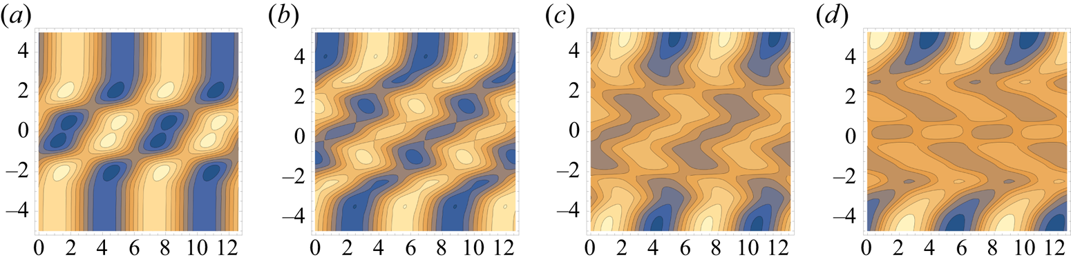
Profiles of (a)  $B_{y}^2\equiv (\partial A/\partial x)^{2}$ and (b) $B_{x}^2\equiv (\partial A/\partial y)^{2}$ for $t=10$ (green), 150 (blue), 500 (red) and 750 (purple).

For the corresponding problem for the scalar field  $\theta$ at Péclet number $Pe=2000$, the field is effectively homogenised in the shearing region by the same time $t\sim 750$.
8. Magnetic relaxation
Magnetic relaxation is a means by which magnetostatic equilibria of arbitrarily prescribed field topology may be determined. Through the  $\boldsymbol {B}$- $\boldsymbol {u}$ analogy (§ 7.2), this is also a means of determining steady Euler flows of arbitrary streamline topology. The idea is to construct a process in which the magnetic energy decreases monotonically, while the field topology is conserved. Obviously the frozen-field equation,
 \begin{equation} \frac{\partial\boldsymbol{B}}{\partial t}=\boldsymbol{\nabla} \times ({\boldsymbol{u}} \times \boldsymbol{B}), \end{equation}
must be part of this process; we can then be sure that the topology of  $\boldsymbol {B}$ is conserved, at least for so long as the field remains smooth. We need to couple this with an equation for $\boldsymbol {u}$, that will guarantee decrease of energy. The process will lead to a non-trivial result only if there is a lower bound for magnetic energy $M(t)=\int \boldsymbol {B}^{2}\,\text {d}V/2$, the integral being through the fluid domain. This lower bound is provided by an inequality first stated by Arnold (Reference Arnold1974).
8.1. The Arnold inequality
The Arnold inequality applies to any magnetic field of non-zero helicity  $\mathcal {H}_{M}$, confined to a finite domain $\mathcal {D}$, with $\boldsymbol {B}\boldsymbol {\cdot } \boldsymbol {n}=0$ on the boundary $\delta \mathcal {D}$. With $\boldsymbol {B}=\boldsymbol {\nabla }\times {\boldsymbol {A}}$, we have first the Schwarz inequality
 \begin{equation} \left[\int \boldsymbol{B}\boldsymbol{\cdot} {\boldsymbol{A}}\right]^{2}\,\text{d}V \le \int \boldsymbol{B}^{2}\,\text{d}V \int {\boldsymbol{A}}^{2}\,\text{d}V, \end{equation}
all integrals being over the domain  $\mathcal {D}$. Second, we have a Poincaré inequality obtained by minimising the Rayleigh quotient $\int \boldsymbol {B}^{2}\,\text {d}V/\int {\boldsymbol {A}}^{2}\,\text {d}V$ by calculus-of-variation techniques; this gives
 \begin{equation} \int {\boldsymbol{A}}^{2}\,\text{d}V\le L_\mathcal{D}^2\int \boldsymbol{B}^{2}\,\text{d}V, \end{equation}
where  $L_\mathcal {D}$ is the maximum span of the domain $\mathcal {D}$. Combining (8.2) and (8.3) leads immediately to the inequality
 \begin{equation} 2 M(t) \ge L_\mathcal{D}^{{-}1}|\mathcal{H}_{M}|, \end{equation}
so that, provided  $\mathcal {H}_{M}\ne 0$, this provides the require lower bound on $M(t)$. Moreover equality occurs here only if $\boldsymbol {B}$ is everywhere parallel to $\boldsymbol {A}$, i.e. only if $\boldsymbol {A}$ is a Beltrami field throughout $\mathcal {D}$.
The physical reason for the Arnold inequality (8.4) is clear: the condition  $\mathcal {H}_{M}\ne 0$ implies a non-trivial topology of the $\boldsymbol {B}$-field, in that there must exist some field lines in $\mathcal {D}$ that cannot be shrunk to a point without crossing other field lines, and this is why the magnetic energy cannot be reduced to zero by any kinematically possible volume-preserving flow.
8.1.1. Energy bound for non-trivial linkage; minimum crossing number
The same consideration applies to fields for which the helicity is zero, but the topology is nevertheless non-trivial. Standard examples, the Whitehead link and the Borromean rings, are shown in figure 18. For the Whitehead link, as already recognised by Maxwell (Reference Maxwell1873), the Gauss linking number is zero, despite the obvious non-trivial linkage. Correspondingly, the link helicity (i.e. the helicity ignoring any internal twist in the individual components of the link) is zero. This is because the invariant magnetic flux  $\int _{S}\boldsymbol {B}\boldsymbol {\cdot }\boldsymbol {n}\,{\text {d}}S$ across any orientable surface $S$ spanning either component of the link is zero.
Links for which the link helicity is zero. (a) The Whitehead link; (b) the Borromean rings.

However,  $\int _{S}|\boldsymbol {B}\boldsymbol {\cdot }\boldsymbol {n}|\,{\text {d}}S$ is not zero, and cannot be reduced to zero by any smooth flow. This integral is not invariant because its value may be increased by pulling additional loops across $S$; however, it has a minimum value when any such superfluous loops are withdrawn as in figure 18(a), and this minimum is a topological invariant, which has been formalised by the concept of ‘minimum crossing number’ by Freedman & He (Reference Freedman and He1991). It is this invariant that provides indirectly a minimum energy for the Whitehead-link configuration. Similar considerations of course apply equally to the Borromean configuration of figure 18(b), and indeed to any other configuration consisting of linked flux tubes.
8.1.2. Arnold inequality for unbounded domain
The Arnold inequality requires modification if the domain  $\mathcal {D}$ is unbounded, for then the scale $L_\mathcal {D}$ is undefined. We may suppose, however, that the $\boldsymbol {B}$-field is itself initially of bounded extent (zero outside some sphere $S_R$ of radius $R$, say) and ‘connected’ in the sense that it cannot be separated into disjoint subfields which could in principle be swept far apart from each other. If the support of such a connected field is deformed by fluid flow (e.g. by uniform irrotational strain) to an extent far greater than $2R$, then, although there may be an initial decrease of energy, this will ultimately increase due to field-line stretching. At any rate, we can define a radius $R_1$, say, $(\ge R)$, such that the field energy increases if the support of the field is stretched to a span greater than $2R_1$. Energy reduction can then only be achieved by contraction. It is then reasonable to assert that Arnold's inequality still holds with $L_\mathcal {D}$ replaced by $R_{1}$; a formal proof of this assertion should not be difficult.
8.2. The basic relaxation process
We suppose then that at time  $t=0$, the field $\boldsymbol {B}(\boldsymbol {x}, 0)=\boldsymbol {B}_{0}(\boldsymbol {x})$ has non-trivial topology, but is otherwise arbitrary, and that it evolves according to the frozen-field equation (8.1). We must couple this with a dynamical process which will guarantee reduction of energy. The most obvious such process is given by the Navier–Stokes equation including the Lorentz force $\boldsymbol {j}\times \boldsymbol {B}$, with $\boldsymbol {j}=\boldsymbol {\nabla }\times \boldsymbol {B}$, and including viscosity as the mechanism of energy dissipation. The model may be criticised as being somewhat artificial, through its inclusion of viscosity ( $\nu \ne 0$) but exclusion of resistivity ( $\eta =0$); but, as I have previously observed (Moffatt Reference Moffatt1985), this is a situation in which the end justifies the means!
In this same Machiavellian spirit, we may adopt an even simpler dynamical prescription. Note first that from (8.1) we may derive an equation for  $M(t)=\int \boldsymbol {B}^{2}\,\text {d}V/2$ in the form
 \begin{equation} \frac{{\text{d}}M}{{\text{d}}t}=\int_\mathcal{D}\boldsymbol{j}\boldsymbol{\cdot} ({\boldsymbol{u}}\times\boldsymbol{B})\,{\text{d}}V={-}\int_\mathcal{D}{\boldsymbol{u}}\boldsymbol{\cdot} (\,\boldsymbol{j}\times\boldsymbol{B})\,{\text{d}}V. \end{equation}
Hence, if we simply choose  $\boldsymbol {u}$ to be on average parallel to $\boldsymbol {j}\times \boldsymbol {B}$, then $M(t)$ will be monotonic decreasing. We achieve this by setting
 \begin{equation} {\boldsymbol{u}}=k^{{-}1}(\,\boldsymbol{j}\times\boldsymbol{B}-\boldsymbol{\nabla} p), \end{equation}
with  $k$ a positive constant; the pressure term $-\boldsymbol {\nabla } p$ is necessary to ensure that $\boldsymbol {\nabla }\boldsymbol {\cdot } {\boldsymbol {u}}=0$; the pressure $p$ is then determined by the Poisson equation $\nabla ^{2}p=\boldsymbol {\nabla }\boldsymbol {\cdot }(\,\boldsymbol {j}\times \boldsymbol {B})$. Substituting in (8.5), and using the fact that $\int _\mathcal {D}{\boldsymbol {u}}\boldsymbol {\cdot } \boldsymbol {\nabla } p\,{\text {d}}V=\int _{\partial \mathcal {D}}(\boldsymbol {n}\boldsymbol {\cdot }{\boldsymbol {u}}) p\,{\text {d}}S=0$, we have immediately
 \begin{equation} \frac{{\text{d}}M}{{\text{d}}t}={-}k\int_\mathcal{D}{\boldsymbol{u}}^{2}\,{\text{d}}V ={-}\varPhi(t), \quad \text{say}, \end{equation}
thus exhibiting the desired monotonic decrease of  $M(t)$. This decrease will persist until ${\boldsymbol {u}}\equiv 0$, and then, with $\boldsymbol {B}_{E}(\boldsymbol {x})=\lim \boldsymbol {B}(\boldsymbol {x},t)$ and similarly for $\boldsymbol {j}$ and $p$, (8.6) gives
 \begin{equation} \boldsymbol{j}_{E}\times\boldsymbol{B}_{E}=\boldsymbol{\nabla} p_{E}, \end{equation}
the required equation of magnetostatic equilibrium, for which  $M(t)$ is minimised.
Throughout this relaxation process, which will generally run to  $t=\infty$, the field $\boldsymbol {B}(\boldsymbol {x},t)$ is a frozen-in field, so that all links and knots of flux tubes are conserved. For finite $t$, the flow defines an ‘isotopy’, i.e. a continuous time-dependent mapping of the field of fluid particles via the Lagrangian displacement field $\boldsymbol {a}\rightarrow \boldsymbol {X}(\boldsymbol {a}, t)$, where $\boldsymbol {a}=\boldsymbol {X}(\boldsymbol {a}, 0)$. But here, care is needed, because in the limit $t\rightarrow \infty$ (and only then is the equilibrium (8.8) attained) there is no guarantee that the mapping remains continuous, and indeed tangential field discontinuities are to be expected, as illustrated by the prototypical case of the Hopf link (§ 8.2.2 below).
8.2.1. Topological accessibility
To describe this situation, I introduced the concept of ‘topological accessibility’ (Moffatt Reference Moffatt1985) with the following sense: for the dynamical model (8.6) a field  $\boldsymbol {B}_{E}(\boldsymbol {x})$ is topologically accessible from the field $\boldsymbol {B}_{0}(\boldsymbol {x})$ if it is obtained by distortion of $\boldsymbol {B}_{0}(\boldsymbol {x})$ by a smooth solenoidal velocity field $\boldsymbol {v}(\boldsymbol {x},t)$, $(0 < t < \infty )$, for which the dissipation function $\varPhi (t)$ satisfies $\int _{0}^{\infty }\varPhi (t)\,{\text {d}}t <\infty$ (different dynamical processes will give rise to different forms for $\varPhi (t)$). Topological accessibility is weaker than topological equivalence, because it allows for the appearance of discontinuities in the field $\boldsymbol {B}_{E}(\boldsymbol {x})$ as $t\rightarrow \infty$.
8.2.2. Relaxation of the Hopf link
The prototypical relaxation scenario is illustrated in figure 19 which illustrates the relaxation of two untwisted but linked flux tubes (the ‘Hopf link’) of volumes  $V_1, V_2$ and fluxes $\varPhi _1,\varPhi _2$ say. During relaxation the linkage and these volumes and fluxes are conserved. The Maxwell tension in the $\boldsymbol {B}$-lines (deriving from the $\boldsymbol {j}\times \boldsymbol {B}$-force) leads to contraction of each tube, with increase of cross-section, until in effect they make contact as in figure 19(b), with a tangential discontinuity in the area of contact. This is where the topological constraint begins to ‘bite’. But relaxation does not stop here; for field lines may still be shortened if either flux tube spreads itself round the other as in figure 19(c), there being then two distinct asymptotic states, both axisymmetric. The discontinuity is then a current sheet on the torus of contact.
Relaxation of the Hopf link: (a) two untwisted but linked flux tubes; (b) contracted state when the tubes make contact; (c) fully relaxed axisymmetric state.
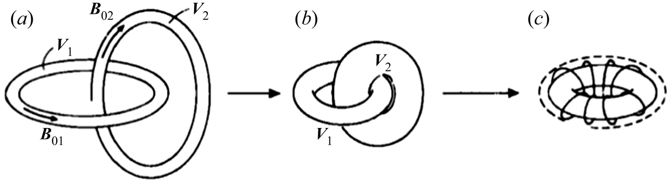
8.2.3. Magnetic relaxation in a compressible medium
The same magnetic relaxation problem can be posed in a compressible fluid, with a barotropic relation  $p=k\rho ^{\gamma }$ between pressure and density (Moffatt Reference Moffatt1987). Magnetostatic equilibrium in such a medium is still governed by (7.3a,b), so the analogy (7.5a–c) is still applicable (the analogous Euler flow still has to be in an incompressible fluid). The limit $k\rightarrow 0$ corresponds to an incompressible fluid for the relaxation process, as considered above, while the limit $k\rightarrow \infty$ corresponds to a pressureless plasma.
The only change is that internal energy has to be taken into account in constructing the relaxation process, but the conclusion is the same: for each  $k> 0$, the field relaxes to a minimum energy magnetostatic equilibrium, and to each such equilibrium there corresponds a steady Euler flow. As I stated in my 1987 paper ‘It is an extraordinary fact that new insights concerning steady flows of a fluid that is (i) inviscid, (ii) incompressible, and (iii) non-conducting, can be obtained through consideration of an unsteady relaxation process in a fluid that is (i) viscous, (ii) compressible, and (iii) perfectly conducting, together with argument by analogy’. Well, perhaps not so extraordinary, but bizarre at the least!
8.2.4. Structure of relaxed state
A relaxed state described by (7.3a,b) is in general severely constrained by the consequence that  $\boldsymbol {B}_{E}\boldsymbol {\cdot }\boldsymbol {\nabla } p_{E}=\boldsymbol {j}_{E}\boldsymbol {\cdot }\boldsymbol {\nabla } p_{E}=0$, so that $\boldsymbol {B}_{E}$-lines and $\boldsymbol {j}_{E}$-lines lie on surfaces $p_{E}= \textrm {const.}$ But what if the $\boldsymbol {B}$-lines are chaotic at the start of the relaxation process (as for the example described in § 4.2 above), and so do not lie on surfaces? Since the $\boldsymbol {B}$-topology is conserved during relaxation, the $\boldsymbol {B}_{E}$-field should also be chaotic, apparently contradicting the requirement that the $\boldsymbol {B}_{E}$-lines should lie on surfaces. We can escape from this constraint in any subdomain $\mathcal {D}_1$ of $\mathcal {D}$ only if $p_{E}\equiv \textrm {const.}$ throughout $\mathcal {D}_1$. But then $\boldsymbol {j}_{E}\times \boldsymbol {B}_{E}=0$ and so $\boldsymbol {j}_{E}=\alpha (\boldsymbol {x})\boldsymbol {B}_{E}$ in $\mathcal {D}_1$, for some scalar function $\alpha (\boldsymbol {x})$. But now, since $\boldsymbol {\nabla }\boldsymbol {\cdot } \boldsymbol {j}_{E}=\boldsymbol {B}_{E}\boldsymbol {\cdot } \boldsymbol {\nabla }\alpha =0$, the $\boldsymbol {B}_{E}$-lines are still constrained to lie on surfaces (now the surfaces $\alpha = \textrm {const.}$). Again, we escape this constraint in any subdomain $\mathcal {D}_2$ of $\mathcal {D}_1$ only if $\alpha = \textrm {const.}$ in $\mathcal {D}_2$. Hence we arrive at the conclusion that if $\boldsymbol {B}_{E}$ is chaotic in any subdomain of $\mathcal {D}$, it must be a Beltrami field, i.e.
 \begin{equation} \boldsymbol{\nabla}\times \boldsymbol{B}_{E}=\alpha \boldsymbol{B}_{E},\quad\alpha=\text{const.} \end{equation}
 Such chaotic Beltrami fields are not unknown; we have seen one example in the ABC flow described in § 4.1. But here we face an extremely challenging problem: as pointed out by Arnold (Reference Arnold1974), there are not nearly enough Beltrami fields, analytic in  $\boldsymbol {x}$ in a given domain $\mathcal {D}$, to cover every conceivable topology that may be adopted for the initial field $\boldsymbol {B}_{0}(\boldsymbol {x})$ of the relaxation process. Of course, as we have seen, discontinuities may develop; but for chaotic fields, it is likely that such discontinuities may become densely stacked throughout the fluid. Bajer (Reference Bajer2005) predicts a ‘devil's staircase’ of such discontinuities, an intriguing idea that calls for further investigation. The problem is as challenging numerically as it is analytically.
8.3. Formation of discontinuities; Parker's model
The formation of discontinuities (current sheets in the magnetostatic situation, vortex sheets in the analogous Euler flow) is of the greatest importance in astrophysical contexts, as discussed by Parker (Reference Parker1994) in his book ‘Spontaneous Current Sheets in Magnetic Fields’ devoted to this topic. Figure 20 shows Parker's basic model: an initially uniform field in a perfectly conducting fluid is distorted by movement of the end points ‘tied’ to the bounding planes  $z=0,L$. The resulting braided structure is supposed relaxed at each instant to a minimum-energy magnetostatic equilibrium, and it is argued that such equilibria must in general exhibit current sheets wherever the distorted flux tubes come in contact. The magnetic relaxation process described above may obviously be adapted to this situation.
Model for the formation of current sheets: movement of the end points of an initially uniform field produces braids of arbitrary complexity (after Parker Reference Parker1994).
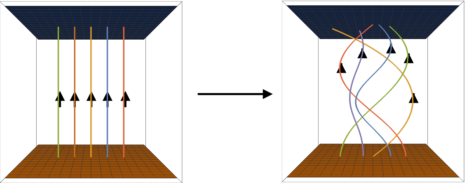
The process is illustrated by just two flux tubes arranged as in figure 21(a). The red tube is part of a helix wound round the straight blue tube. Relaxation causes shortening of the red tube, the end points being fixed, until contact between the tubes, i.e. a tangential discontinuity, occurs, as shown in figure 21(b). The blue tube is also deformed during this relaxation process, due to the motion of the ambient fluid, the amount of this deformation depending on the relative strengths of the two tubes. Relaxation will presumably continue after contact is established; ultimately both tubes will be nearly V-shaped, but still with the same linkage.
Simplified model of the Parker mechanism: two flux tubes, blue and red, span the space between parallel planes; the planes and the fluid are assumed perfectly conducting. Relaxation causes shortening of the red tube, and deformation of the blue tube, the end points being fixed, so that contact between the tubes is inevitable; a current sheet forms on the area of contact.

One may well ask how the configuration of figure 21(a) could arise in the first place, starting from two straight parallel tubes. If the top point of the red tube is wound round the blue tube through an angle  $2 {\rm \pi}$, then, provided the twist is uniformly distributed between the two planes, the configuration of figure 21(a) will result. This uniform distribution, however, requires a linear (Couette) velocity distribution between the planes, which in turn requires viscosity. But even if the distribution of twist is non-uniform, relaxation will still always lead to contact, provided the angle of twist at the upper boundary is greater than ${\rm \pi}$. In practice, winding and relaxation will occur simultaneously; if the relaxation occurs on a much shorter time scale than the winding, then the field will be permanently in a nearly minimum-energy state (with or without tangential discontinuities), as in effect assumed by Parker.
Current sheets are the source of strong plasma heating due to ohmic dissipation, a favoured mechanism for the heating of the solar corona to temperatures of order  $10^{6}\ \textrm {K}$; here, the magnetic field is ‘anchored’ at the photospheric surface, and the footpoints move in response to sub-surface turbulence. Current sheets in the relaxed coronal field are an inevitable consequence. Kinematic viscosity $\nu =\mu /\rho$ is many orders of magnitude greater than $\eta$ in the corona because of the extremely high temperature and the low particle number density $n=10^{15}\ \textrm {m}^{-3}$; Craig & Litvinenko (Reference Craig and Litvinenko2009) estimate $\nu /\eta \sim 10^{10}$, although they also warn that the viscous stress tensor is strongly anisotropic in this very diffuse magnetised medium. Much work on braided magnetic fields has been stimulated by the Parker model (see particularly Wilmot-Smith, Pontin & Hornig Reference Wilmot-Smith, Pontin and Hornig2010; Pontin et al. Reference Pontin, Wilmot-Smith, Hornig and Galsgaard2011).
8.4. Relaxation to magnetodynamic states
The method of magnetic relaxation to magnetostatic equilibria can be extended to the problem of determining steady solutions of the full magnetohydrodynamic equations in an ideal fluid  $(\nu =\eta =0)$, having prescribed magnetic field topology and prescribed interlinkage of vorticity and magnetic fields. This requires conservation of all magnetic helicity integrals and also all ‘cross-helicity’ integrals
 \begin{equation} \mathcal{H}_{C}({\mathcal{D}_{L}})=\int_{\mathcal{D}_{L}} {\boldsymbol{u}}\boldsymbol{\cdot} \boldsymbol{B}\,{\text{d}}V, \end{equation}
where  $\mathcal {D}_{L}$ is any Lagrangian subdomain on whose surface $\boldsymbol {n}\boldsymbol {\cdot }\boldsymbol {B}=0$. We assume that $|\mathcal {H}_{C}(\mathcal {D})|\ne 0$; then a lower bound on energy is provided by the Schwarz inequality
 \begin{equation} \int_\mathcal{D} {\tfrac{1}{2}}({\boldsymbol{u}}^2 +\boldsymbol{B}^2)\,{\text{d}}V \ge \left|\int_\mathcal{D} {\boldsymbol{u}}\boldsymbol{\cdot} \boldsymbol{B}\,{\text{d}}V\right|= |\mathcal{H}_{C}(\mathcal{D})|. \end{equation}
A relaxation process has been constructed by Vladimirov, Moffatt & Ilin (Reference Vladimirov, Moffatt and Ilin1999) satisfying these topological constraints. The end result of this relaxation process is a velocity field  $\boldsymbol {U}(\boldsymbol {x})$ and magnetic field $\boldsymbol {B}(\boldsymbol {x})$ that satisfy the steady equations of ideal magnetohydrodynamics, which may be expressed in the form
 \begin{equation} \boldsymbol{U}\times \boldsymbol{B}=\boldsymbol{\nabla}\varPhi,\quad \boldsymbol{U}\times \boldsymbol{\varOmega} + \boldsymbol{J}\times \boldsymbol{B}=\boldsymbol{\nabla} h, \end{equation}
where  $h=p +\boldsymbol {U}^2/2, \boldsymbol {\varOmega }=\boldsymbol {\nabla }\times \boldsymbol {U}, \boldsymbol {J}=\boldsymbol {\nabla }\times \boldsymbol {B}$. It is not difficult to show that, if the initial fields are chaotic in this situation then the relaxed fields must satisfy
 \begin{equation} \boldsymbol{\varOmega}=\beta \boldsymbol{U}=\alpha \boldsymbol{J}=\alpha\beta\,\boldsymbol{B}, \end{equation}
where  $\alpha$ and $\beta$ are constants. Again, these relaxed chaotic Beltrami fields must presumably incorporate an incalculable profusion of discontinuities.
9. Stability
As already indicated, the analogy (7.5a–c) is limited to steady states, but does not extend to unsteady perturbations about these states. For the magnetostatic equilibria, such perturbations involve frozen-field deformation of the  $\boldsymbol {B}$-field, or so-called ‘isomagnetic’ perturbations. We must imagine an ‘isomagnetic foliation’ of the function space of $\boldsymbol {B}$-fields, as in figure 22, a $\boldsymbol {B}$-field being constrained to evolve on a single folium.
Conceptual representation of the foliations of the (infinite-dimensional) function space of the  $\boldsymbol {B}$- or $\boldsymbol {U}$-fields; pink represents the isomagnetic foliation; blue the isovortical foliation. Stability criteria are different for isomagnetic or isovortical perturbations.
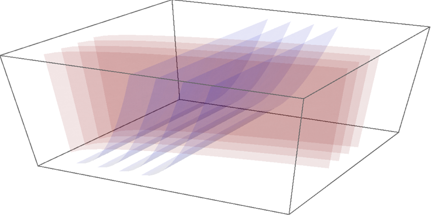
For the analogous Euler flow, it is the vorticity field that is frozen under perturbations governed by the Euler equations; so we must similarly imagine an ‘isovortical foliation’ of the same functions space, which is distinct from the isomagnetic foliation. Perturbations on the two foliations can behave quite differently.
9.1. Stability of magnetostatic equilibria
A magnetostatic equilibrium in a perfectly conducting fluid is stable if its magnetic energy  $M_{E}=\int \boldsymbol {B}_{E}^2\,{\text {d}}V/2$ is minimal with respect to isomagnetic perturbations. We may think of a ‘virtual displacement’ $\boldsymbol {\xi } (\boldsymbol {x},\tau )$ as the Lagrangian displacement associated with a virtual steady velocity field $\boldsymbol {v}(\boldsymbol {x})$, as sketched in figure 23. When this displacement is small, as evident from the sketch, the associated Eulerian displacement $\boldsymbol {\eta }(\boldsymbol {x})$, satisfying $\boldsymbol {\nabla }\boldsymbol {\cdot }\boldsymbol {\eta }=0$, is given by
 \begin{equation} \boldsymbol{\eta}(\boldsymbol{x})=\boldsymbol{\xi} -{\tfrac{1}{2}} \boldsymbol{\xi} \boldsymbol{\cdot}\boldsymbol{\nabla} \boldsymbol{\xi} +{O}(\boldsymbol{\xi})^2. \end{equation}
With this displacement, the field  $\boldsymbol {B}_{E}(\boldsymbol {x})$ is distorted to $\boldsymbol {B}(\boldsymbol {x}) = \boldsymbol {B}_{E}(\boldsymbol {x}) +\delta ^{1}\boldsymbol {B} +\delta ^{2}\boldsymbol {B}+{O}(|\boldsymbol {\eta }|^3)$, where
 \begin{equation} \delta^{1}\boldsymbol{B}=\boldsymbol{\nabla}\times(\boldsymbol{\eta}\times\boldsymbol{B}_{E}),\quad \delta^{2}\boldsymbol{B}={\tfrac{1}{2}}\boldsymbol{\nabla}\times(\boldsymbol{\eta}\times\delta^{1}\boldsymbol{B}), \end{equation}
and the perturbed magnetic energy is then  $M=M_{E}+\delta ^{1}M+\delta ^{2}M+{O}(|\boldsymbol {\eta }|^3)$, where
 \begin{equation} \delta^{1}M=\int [\boldsymbol{B}_{E}\boldsymbol{\cdot}\delta^{1}\boldsymbol{B}]\,\text {d}V,\quad \delta^{2}M={\tfrac{1}{2}}\int[(\delta^{1}\boldsymbol{B})^2+2\boldsymbol{B}_{E}\boldsymbol{\cdot}\delta^{2}\boldsymbol{B}]\,\text{d}V. \end{equation}
It is not difficult to show that, by virtue of (7.3a,b), the first variation  $\delta ^{1}M$ is zero, as might be expected for an equilibrium state. The expression for $\delta ^{2}M$ may then be manipulated to the form
 \begin{equation} \delta^{2}M={\tfrac{1}{2}}\int[(\boldsymbol{\nabla}\times(\boldsymbol{\eta}\times\boldsymbol{B}_{E}))^2-(\boldsymbol{\eta}\times\boldsymbol{j}_{E}\boldsymbol{\cdot}(\boldsymbol{\nabla}\times(\boldsymbol{\eta}\times\boldsymbol{B}_{E}))]\,\text{d}V. \end{equation}
Stability is then assured if  $\delta ^{2}M\ge$ for all ‘admissible displacements’ $\boldsymbol {\eta }(\boldsymbol {x})$, i.e. those satisfying $\boldsymbol {\nabla }\boldsymbol {\cdot }\boldsymbol {\eta }=0$ in the relevant domain $\mathcal {D}$, and $\boldsymbol {n}\boldsymbol {\cdot } \boldsymbol {\eta }=0$ on $\partial \mathcal {D}$.
Sketch indicating the relation between the Lagrangian displacement  $\boldsymbol {\xi } (\boldsymbol {x},\tau )$ induced by a virtual velocity field $\boldsymbol {v}(\boldsymbol {x})$ and the associated Eulerian displacement $\boldsymbol {\eta }$ after a short time $\tau$; these displacement functions are related as in (9.1).

For this result to be useful, it is necessary to put a bound on the term  $\int \boldsymbol {B}_{E}\boldsymbol {\cdot }\delta ^{2}\boldsymbol {B}\,\text {d}V$ in (9.3a,b). This involves identifying the lowest positive eigenvalue $\lambda$ of a rather complicated eigenvalue problem, and leads to the result
 \begin{equation} \delta^{2}M\ge {\tfrac{1}{2}}\left(1-\lambda^{{-}1/2}\right)\int\left[\left(\delta^{1}\boldsymbol{B}\right)^2\right]\,\text{d}V, \end{equation}
so that the condition  $\delta ^{2}M\ge 0$ simply requires that $\lambda \ge 1$. A result of this kind was first found by Bernstein et al. (Reference Bernstein, Frieman, Kruskal and Kulsrud1958); details of the above derivation may be found in Moffatt (Reference Moffatt1986). Of course, as already observed, magnetostatic equilibria obtained by the method of magnetic relaxation are stable, and must then automatically satisfy the condition $\delta ^{2}M\ge 0$.
9.2. Instability of analogous Euler flows
Consider now a steady Euler flow  ${\boldsymbol {u}}_{E}(\boldsymbol {x})$ in $\mathcal {D}$, with kinetic energy $K_{E}=\int {\boldsymbol {u}}_{E}^2\,{\text {d}}V/2$. Just as for the magnetostatic equilibrium, we may (following Arnold Reference Arnold1965b) investigate the stability of this flow by considering the second variation of ${\boldsymbol {u}}_{E}(\boldsymbol {x})$, but now with respect to the isovortical perturbations permitted by the Euler equations. It is now therefore the vorticity $\boldsymbol {\omega }=\boldsymbol {\nabla }\times {\boldsymbol {u}}$ that is given by ${\boldsymbol {\omega }}(\boldsymbol {x}) = {\boldsymbol {\omega }}_{E}(\boldsymbol {x}) +\delta ^{1}{\boldsymbol {\omega }} +\delta ^{2}{\boldsymbol {\omega }}+{O}(|\boldsymbol {\eta }|^3)$, where
 \begin{equation} \delta^{1}{\boldsymbol{\omega}}=\boldsymbol{\nabla}\times(\boldsymbol{\eta}\times{\boldsymbol{\omega}}_{E}),\quad \delta^{2}{\boldsymbol{\omega}}={\tfrac{1}{2}}\boldsymbol{\nabla}\times(\boldsymbol{\eta}\times\delta^{1}{\boldsymbol{\omega}}), \end{equation}
or, by ‘uncurling’,  ${\boldsymbol {u}}(\boldsymbol {x})= {\boldsymbol {u}}_{E}(\boldsymbol {x}) +\delta ^{1}{\boldsymbol {u}} +\delta ^{2}{\boldsymbol {u}}+{O}(|\boldsymbol {\eta }|^3)$, where
 \begin{equation} \delta^{1}{\boldsymbol{u}}=(\boldsymbol{\eta}\times{\boldsymbol{\omega}}_{E})_{s},\quad \delta^{2}{\boldsymbol{u}}={\tfrac{1}{2}}(\boldsymbol{\eta}\times\delta^{1}{\boldsymbol{\omega}})_{s}, \end{equation}
and where the suffix  $s$ denotes the ‘solenoidal projection’, required to ensure that $\boldsymbol {\nabla }\boldsymbol {\cdot } \delta ^{1}{\boldsymbol {u}}=\boldsymbol {\nabla }\boldsymbol {\cdot } \delta ^{2}{\boldsymbol {u}}=0$.
Again it may be shown that the first variation  $\delta ^{1}K$ of kinetic energy is zero by virtue of the equilibrium condition (7.4a–c); and for admissible $\boldsymbol {\eta }$ the second variation $\delta ^{2}K$ may be expressed in the form
 \begin{align} \delta^{2}K& ={\tfrac{1}{2}}\int[(\delta^{1}{\boldsymbol{u}})^{2}+2{\boldsymbol{u}}_{E}\boldsymbol{\cdot}\delta^{2}{\boldsymbol{u}}]\,{\text{d}}V\nonumber\\&={\tfrac{1}{2}}\int[(\boldsymbol{\eta}\times\boldsymbol{\omega}_{E})_{s}^{2}-(\boldsymbol{\eta}\times\boldsymbol{\omega}_{E})_{s}\boldsymbol{\cdot}\boldsymbol{\nabla}\times(\boldsymbol{\eta}\times{\boldsymbol{u}}_{E})]\,{\text{d}}V. \end{align}
There is an obvious difference between this expression for  $\delta ^{2}K$ and $\delta ^{2}M$ as given by (9.4); it is this difference that accounts for the different stability properties of magnetostatic equilibria and their analogous Euler flows. This is most easily illustrated by the following simple example.
9.3. Two-dimensional cylindrical equilibria
Consider the magnetostatic equilibrium and the analogous Euler flow
 \begin{equation} \boldsymbol{B}^{E}=(0,b(r),0),\quad \boldsymbol{v} ^{E}=(0,v(r),0), \end{equation}
in cylindrical polar coordinates  $(r,\theta , z)$. We may take $\mathcal {D}$ to be the domain $a_1 < r < a_2, 0 < z < z_{1}$, the boundary $\partial \mathcal {D}$ being perfectly conducting. We may consider the stability of these states to admissible axisymmetric disturbances of the form $\boldsymbol {\eta }=(\eta _r,0,\eta _z)=r^{-1}(\partial \psi /\partial z, 0, -\partial \psi /\partial r)$, with $\psi =0$ on $\partial \mathcal {D}$. The expressions (9.4) for $\delta ^{2}M$ and (9.8) for $\delta ^{2}K$ may in this case be reduced and manipulated to the form
 \begin{equation} \delta^{2}M={-}{\rm \pi}\iint\eta_{r}^{2}\frac{\text{d}}{{\text{d}}r}\left(\frac{b}{r}\right)^{2}r^{2}\,{\text{d}}r\,{\text{d}}z,\quad \delta^{2}K=2{\rm \pi}\iint\eta_{r}^{2}\frac{\text{d}}{{\text{d}}r}({r v})^{2}r^{{-}2}\,{\text{d}}r\,{\text{d}}z. \end{equation}
Thus, if  $(b/r)^2$ is a monotonic decreasing function of $r$ throughout the range $a_1 < r < a_{2}$, then $M$ is minimal at $M=M_E$, and so the magnetostatic equilibrium $\boldsymbol {B}^{E}$ is stable. We may note that this result may be most simply obtained by considering the energy needed to interchange two flux tubes of the same volume at different radii $r_{1} < r_{2}$, say, the flux in each tube being constant: the energy needed for the interchange is then proportional to $[b(r_{1})/r_{1}]^2-[b(r_{2})/r_{2}]^2$, and if this is positive, the equilibrium is stable, at least to axisymmetric perturbations of the kind considered.
Similarly,  $K$ is minimal at $K=K_{E}$ if $(rv)^2$ is an increasing function of $r$, i.e. if the circulation $2{\rm \pi} |rv (r)|$ increases outwards; this is just the sufficient condition for stability known as Rayleigh's criterion (Rayleigh Reference Rayleigh1917). Equally, a necessary condition for instability of the analogous Euler flow is that the circulation should decrease outwards. Thus for example, if both $b(r)$ and $v(r)$ are proportional to $r^{-3/2}$, then $(b(r)/r)^2$ and $(rv(r))^2$ are both monotonic decreasing functions of $r$, so that the magnetostatic equilibrium is stable, whereas the analogous Euler flow satisfies the necessary condition for instability.
9.3.1. Arnold's assertion and its refutation
We pause here to comment on the assertion of Arnold (Reference Arnold1965b) that an Euler flow  ${\boldsymbol {u}}_{E}(\boldsymbol {x})$ should be stable if its kinetic energy $K_{E}$ is extremal (i.e. either minimal or maximal) with respect to isovortical perturbations. The assertion was based on the idea that under unsteady Euler evolution, the kinetic energy $K$ is a conserved quantity, and if $K$ is extremal at $K=K_{E}$, then $K$ must always remain close to $K_{E}$ when the Euler flow is slightly disturbed. This statement holds whether $K$ is minimal or maximal at $K_{E}$; but the simple example described above indicates that the flow is stable if $K$ is minimal, but potentially unstable if $K$ is maximal at $K_{E}$. So where is the fallacy in Arnold's argument?
The answer is this: when  $K$ is minimal at $K_{E}$, it requires a small instantaneous injection of energy to perturb the flow away from the equilibrium. It then does indeed remain close to $K_{E}$, and the perturbation cannot grow (without further injection of energy). When $K$ is maximal at $K_{E}$, the situation is very different: a perturbation can grow at the expense of energy extracted from the ‘base’ flow. The total energy (i.e. the energy of the base flow plus the energy of the perturbation) does indeed remain constant, but the base flow can continue to lose energy to the disturbance, so that instability can progress unhindered, until some kind of equilibrium between the base flow and the growing (finite-amplitude) perturbation can be established.
9.3.2. Rayleigh's criterion, as anticipated by Maxwell
Rayleigh's criterion for instability (that ‘the circulation must decrease outwards’) was actually anticipated by James Clerk Maxwell in a problem that he posed as an External Examiner for the Mathematical Tripos at Cambridge University in 1866. This may be found in Volume II of the Scientific Papers and Letters of James Clerk Maxwell (Harman Reference Harman1995) as a ‘Draft question on the stability of vortex motion’:
A mass  $M$ of fluid is running round a circular groove or channel of radius $a$ with velocity $u$. An equal mass is running round another channel of radius $b$ with velocity $v$. The one channel is made to expand and the other to contract till their radii are exchanged. Show that the work expended in effecting the change is
 \[ -\frac{1}{2}\left(\frac{u^2} {b^2} - \frac{v^2} {a^2}\right)( a^2- b^2)M.\]
Hence show that the motion of a fluid in a circular whirlpool will be stable or unstable according as the areas described by particles in equal times increase or diminish from centre to circumference.
The final sentence of this question (the sting in the tail!) is particularly noteworthy, as being essentially equivalent to Rayleigh's criterion, evidently known to Maxwell some 50 years earlier! The word ‘circulation’ had not entered the literature of hydrodynamics in 1866, but Maxwell's ‘area described by a particle’ in time  $\delta t$ is just $(r^{2}(v/r) \delta t)/2=rv \delta t/2$, so proportional to circulation. Interesting that Maxwell should start here from a simple thought experiment, and then broaden to a general principle!
9.3.3. Three-dimensional instability of Euler flows
Returning to the general expression (9.8) for  $\delta ^{2}K$, it was shown by Rouchon (Reference Rouchon1991) that if attention is focused on three-dimensional perturbation displacements $\boldsymbol {\eta }(\boldsymbol {x})$ of sufficiently small scale, it is the second term in the integral that dominates (because, unlike the first term, this involves the derivative of $\boldsymbol {\eta }$), and that if $\boldsymbol {\eta }^{+}(\boldsymbol {x})$ is a (small-scale) choice for which $\delta ^{2}K>0$, then there always exists an alternative choice $\boldsymbol {\eta }^{-}(\boldsymbol {x})$ for which $\delta ^{2}K<0$. The implication is that Arnold's condition for the stability of Euler flows is never satisfied if the full range of three-dimensional admissible displacement functions is considered. The Euler flows must thus be considered as saddle points (rather than extrema) in the function space available to them.
Rouchon assumed these flows to be at least  $\mathbb {C}^{2}$, i.e. twice continuously differentiable; but there seems little doubt that his result extends to Euler flows that admit tangential discontinuities, and as we have seen, this is likely to be typical for non-trivial three-dimensional flows. Instabilities of Kelvin–Helmholtz type are indeed to be expected in the neighbourhood of such discontinuities.
9.4. Kelvin modes and transient growth
Even when a flow of a viscous fluid, such as plane Couette flow, is stable to infinitesimal disturbances, it may nevertheless exhibit significant growth of disturbances before these are ultimately eliminated by viscosity. This type of behaviour, known as ‘transient growth’ (or sometimes ‘transient instability’) is most simply illustrated by the following model (Moffatt Reference Moffatt1967).
We suppose that a weak disturbance of the form  ${\boldsymbol {u}}(\boldsymbol {x},0)={\boldsymbol {A}}_{0}\exp {[\text i}\boldsymbol {k}_{0}\boldsymbol {\cdot } \boldsymbol {x}]$ with $\boldsymbol {k}_{0}\boldsymbol {\cdot } {\boldsymbol {A}}_{0}=0$ is superposed at time $t=0$ on a uniform shear flow $\boldsymbol {U}=(\alpha y, 0,0)$. The linearised Navier–Stokes equation
 \begin{equation} \frac{\partial{\boldsymbol{u}}}{\partial t}+{\boldsymbol{u}}\boldsymbol{\cdot} \boldsymbol{\nabla} \boldsymbol{U}+\boldsymbol{U}\boldsymbol{\cdot} \boldsymbol{\nabla} {\boldsymbol{u}}={-}\frac{1}{\rho}\boldsymbol{\nabla} p +\nu \nabla^{2}{\boldsymbol{u}}, \end{equation}
where  $p(\boldsymbol {x}, t)$ is the pressure field and $\rho$ is the (constant) fluid density, admits ‘Kelvin wave’ solutions of the form $[{\boldsymbol {u}}, p/\rho ] ={[\boldsymbol {A}}(t), P(t)] \exp {[\text i}\boldsymbol {k}(t)\boldsymbol {\cdot }\boldsymbol {x}]$, where $\boldsymbol {k}(t)=(k_{01},k_{02}-\alpha t \,k_{01}, k_{03})$. The effect of the shear is to tilt the wave fronts progressively in a clockwise sense until the normal to these wavefronts is nearly parallel to the $y$-axis.
The effect of viscosity is to provide a damping factor  $D(t)$ for the wave amplitude, where
 \begin{equation} D(t)=\exp\left[-\nu\int\boldsymbol{k}^{2}(t)\,{\text{d}}t\right]= \exp\left[-\nu\left(k_{0}^{2}t-k_{01}k_{02}\alpha t^2 +{\tfrac{1}{3}} k_{01}^{2}\alpha^2 t^3\right)\right]. \end{equation}
This damping is ultimately responsible for the decay of the wave disturbance; if  $k_{01}\ne 0$, then for large $\alpha t$, $D(t)\sim \exp [-(\nu k_{01}^{2}\alpha ^2 t^3/3)]$, so that the wave decays on a time scale $t_{\nu }=(\nu k_{01}^{2}\alpha ^2)^{-1/3}$ (cf. the Rhines & Young time scale encountered in § 7.2). We assume here that $\nu$ is small, and focus on the development for $t \ll t_{\nu }$; during this stage, we may simply set $\nu =0$.
Elimination of the pressure term leads to a dynamical system for the amplitude components
 \begin{align} \frac{{\text{d}}{A_{1}}}{{\text{d}}t}+\alpha A_{2}=\frac{2\alpha A_{2}k_{01}^{2}}{{|\boldsymbol{k}}(t)|^{2}},\quad\frac{{\text{d}}{A_{2}}}{{\text{d}}t}=\frac{2\alpha A_{2}k_{01}(k_{02}-\alpha t k_{01})}{{|\boldsymbol{k}}(t)|^{2}},\quad \frac{{\text{d}}{A_{3}}}{{\text{d}}t}=\frac{2\alpha A_{2}k_{01}k_{03}}{{|\boldsymbol{k}}(t)|^{2}}, \end{align}
which may be solved explicitly for the components  $A_{1}(t), A_{2}(t), A_{3}(t)$. Typical behaviour is shown in figure 24(a) for initial conditions $\boldsymbol {k}(0)=(0.3, 1,0.5), {\boldsymbol {A}}(0)=(0.1, 0.5, -0.53)$ (red) and $\boldsymbol {k}(0)=(0.1, 1,0.5), {\boldsymbol {A}}(0)=(0.1, 0.5, -0.51)$ (blue). It is evident that $A_{1}(t)$ exhibits a relatively long period of linear growth when $k_{10}$ is small; this is the key characteristic of transient growth.
Transient instability;  $k_{20}=1,k_{30}=0.5$; $A_{1}(0)=0.11,A_{2}(0)=0.5$ (a) $\varepsilon =0$; $k_{10}=0.3,$ (red), $0.1$ (blue); $A_{1}(t)$ (solid), $A_{2}(t)$ (dashed), $A_{3}(t)$ (dotted); the transient instability shows in $A_{1}(t)$ and becomes more marked as $k_{10}$ decreases. (b) Effect of viscosity; $k_{10}=0.1$; $\varepsilon = Re^{-1} =10^{-2}$ (red), $10^{-3}$ (green), $10^{-4}$ (purple), $0$ (blue); as $\varepsilon$ decreases, the curves shadow the inviscid limit (blue) for an increasing period of time, but ultimately diverge from it and asymptote to zero.

Figure 24(b) shows the effect of viscosity on the component  $A_{1}(t)$ for the case $k_{10}=0.1$ through the dimensionless parameter $\varepsilon =\nu k_{02}^{2}/\alpha$ (an inverse Reynolds number) when the decay factor $D(t)$ is restored. As $\varepsilon$ decreases, the solution shadows the inviscid solution (shown again in blue) more and more closely, but ultimately diverges from this solution and decays to zero through the effect of viscosity.
If the perturbation vorticity is random it can be Fourier analysed, and it is then the ingredients with  $k_{1}$ small that are subject to this type of transient growth, the associated streamwise component $v_1$ being then amplified linearly in time. This is believed to be the cause of the ‘streamwise rolls’ that are frequently observed in shear-flow turbulence. It is probably also the cause of the ‘streaks’ observed in the laminar sublayer of a turbulent boundary layer (Kline et al. Reference Kline, Reynolds, Schraub and Runstadler1967). In both cases, these strong streamwise motions are unstable to three-dimensional instabilities that provide a powerful trigger for the generation and maintenance of turbulence.
10. Knotted flux tubes
The magnetic relaxation procedure described in § 8 can be applied to the particular case of knotted flux tubes, with results that have some relevance for the general problem of ‘knot energy’ and associated knot invariants. Thus, let  $K$ be an arbitrary knot of length $L$ in some arbitrary geometrical configuration defined by the closed curve $C$. We imagine this to be imbedded in a viscous, perfectly conducting, incompressible fluid, and that a magnetic flux tube $\textit {T}$ of flux $\varPhi$ and of cross-sectional radius $\delta$ is placed in a ‘tubular neighbourhood’ of $C$, where $\delta$ is small compared with the minimum curvature of $C$. For simplicity, we may assume that the axial magnetic field has a simple ‘top-hat’ profile over the cross-section of $\textit {T}$. The volume of the flux tube is $V\sim LA$, where $A={\rm \pi} \delta ^2$, and the magnetic energy associated with the axial field component is $M_0 \sim (\varPhi /A)^2 V/2$.
10.1. Knot helicity, writhe and twist
The helicity  $\mathcal {H}$ of the field distribution must, for dimensional reasons, have the form $\mathcal {H} = h \varPhi ^2$ where $h$ is dimensionless and (like $\mathcal {H}$ and ${\varPhi }$) invariant under continuous deformation of the tube $\textit {T}$. This helicity arises in part from the knot topology, but also in part from the amount of internal twist of the magnetic field within the flux tube. In fact $h$ can be changed by a ‘cut, twist, reconnect’ process: cut the tube, twist one end through an angle $2{\rm \pi} \Delta h$ and reconnect the tube; the helicity of the field will then be changed by $\pm \Delta h \varPhi ^2$, the sign depending on the sense (right- or left-handed) of the twist. In particular, we may always choose $\Delta h$ to make $h=0$; this is what is known as ‘zero framing’ of the knot.
It was shown by Moffatt & Ricca (Reference Moffatt and Ricca1992) that  $h=Wr+Tw$, where $Wr$ and $Tw$ are the writhe and twist of $\textit {T}$. We have already encountered writhe and twist in § 6.3.2; these vary continuously under continuous deformation, their sum being constant. The writhe is given by (6.15), and can be interpreted as the sum of the signed crossings of the knot, averaged over all projections. The twist $Tw$ consists of two parts: $Tw=\mathcal {T}+\mathcal {N}$. Here, $\mathcal {T}=(2{\rm \pi} )^{-1}\oint _{C} \tau (s,t)\, {\text {d}}s$, where $\tau (s,t)$ is the torsion on the curve at arc-length position $s$; and $\mathcal {N}$ is the ‘internal twist’ within the tube $\textit {T}$, i.e. the number of turns of the normal on a ribbon bounded by any two field line in the tube relative to the Frenet triad $\{{\boldsymbol {t}, \boldsymbol {n}, \boldsymbol {b}}\}$ on $C$. As evident from the example described in § 6.3.2, $\mathcal {T}$ and $\mathcal {N}$ have equal and opposite unit jumps if the curve $C$ is deformed through an inflexional configuration, but the sum $Tw=\mathcal {T}+\mathcal {N}$ varies continuously. The relevance of writhe and twist in biophysical contexts was well described by Crick (Reference Crick1976), who discussed in particular the writhe and twist of closed, circular, supercoiled DNA molecules.
10.2. The energy spectrum of knots and links
We now let the knot magnetic field relax to a minimum-energy state following the procedure of § 8. The Lorentz force manifests itself as Maxwell tension in the field lines, which causes the flux tube to shrink in length. During this process,  $\varPhi$ is conserved by virtue of the assumed perfect conductivity; and $V$ is conserved by incompressibility, so that $A\sim V/L$ must increase as $L$ decreases. Hence, if the knot $K$ is non-trivial, it must eventually come into contact with itself. It is at this stage that the knot topology ‘bites’ leading ultimately to a magnetostatic equilibrium in which $L\sim V^{1/3}$ and $A\sim V^{2/3}$. In this equilibrium, the magnetic energy is minimal and proportional to $\varPhi ^2 V^{-1/3}$. This minimum energy $M_{{min}}$ can (and does) depend also on $h$; hence we must have
 \begin{equation} M_{{min}} = m(h)\varPhi^2 V^{{-}1/3}, \end{equation}
where the dimensionless function  $m(h)$ is determined solely by the knot $K$ (Moffatt Reference Moffatt1990).
The situation is illustrated in figure 25(a), which shows a schematic of the relaxation of the trefoil knot  $T_{2,3}$ to its minimum-energy state, in which it makes contact with itself presumably over a ‘surface of contact’ $S_{c}$. The notation $T_{n, m}$ is used here to indicate a torus knot that embraces the small circuit of the torus $m$ times, and the large circuit $n$ times. The knot $T_{n, m}$ is topologically equivalent to $T_{m, n}$ (i.e. can be continuously deformed to this configuration). Figure 25(b) shows relaxation of $T_{3, 2}$ to its minimum-energy state, with obviously different symmetry from that of $T_{2,3}$. It is thus clear that the minimum-energy state is not unique. In general, we must anticipate that, for any given knot $K$, there may exist a sequence of minimum-energy states, with energy functions
 \begin{equation} \{m_{0}(h), m_{1}(h), m_{2}(h), \ldots\}, \end{equation}
which may be ordered so that  $m_{0}(0) \le m_{1}(0) \le m_{2}(0) \le \cdots$; it seems natural to describe the sequence (10.2) as the ‘energy spectrum’ of the knot $K$. The whole approach is equally applicable to links, with minor modifications.
(a) Schematic of the relaxation of the trefoil knot  $T_{2,3}$ to its minimum energy state; and (b) of the same knot in the configuration $T_{3,2}$ to a different minimum-energy state.

The energy function  $m(h)$ was obtained by a minimisation procedure by Chui & Moffatt (Reference Chui and Moffatt1995) for four torus knots $T_{m, n}$ with $m=2,\, n=3,5,7,9$, as shown in figure 26. In this derivation, it was assumed that the tube cross-section was constrained to remain circular, that the tubes were in their simplest configurations (with $n$-fold symmetry), and that the helicity density was uniform throughout the tube volume. The minima of these curves occur for $h > 0$, reflecting the chirality of the torus knots considered. (For the trefoil $T_{2, 3}$, the minimum is at $h\approx 6$, where $m_{min}\approx 32$.) Moreover, as might be expected, for modest values of $h (\lesssim 10)$, $m(h)$ increases with increasing $n$, i.e. with increasing knot complexity. More surprisingly, this ordering changes for larger values of $h$; however, for $|h|\gg 1$ the tubes are subject to ‘kink-mode’ instabilities which break the $n$-fold symmetries, thus lowering the minimum-energy curves by an as yet undetermined amount.
Minimum-energy curves for four torus knots; the minima occur for  $h>0$, reflecting knot chirality; for small $h$,
$h$,  $m(h)$ increases with increasing knot complexity. (From Chui & Moffatt Reference Chui and Moffatt1995.)

10.3. The analogue Euler knots
The relaxed magnetic-flux-tube knots described above are stable insofar as the fluid can be considered perfectly conducting, being minimum-energy magnetostatic equilibria. The analogous steady Euler flows derived via the substitutions (7.5a–c) involve helical flow along the knotted tube, with a tangential discontinuity of velocity (i.e. a vortex sheet) on the surface of contact  $S_{c}$. This vortex sheet, although curved and of limited extent, is presumably unstable to Kelvin–Helmholtz modes of short wavelength. Kelvin, in proposing his ‘vortex atom’ theory in 1867, had hoped to find solutions of the Euler equations representing stable knotted vortices, but was thwarted in this search, in part because of the all-pervasive influence of such instabilities.
Magnetic vortex knots do not suffer such instabilities, and would have provided a better candidate for Kelvin's speculations, had he but known of the frozen-in character of the magnetic field in a perfectly conducting fluid. Although the fundamental ingredients (the Euler and Maxwell equations) were already available by 1870, the implications for magnetohydrodynamics were not recognised till the much later work of Alfvén (Reference Alfvén1946); but by then Kelvin's concept of microscopic vortical disturbances in a hypothetical ethereal medium had been consigned to oblivion.
10.4. Tight knots
The relaxed states shown in figure 25 have the appearance of ‘tight knots’, imagined as trefoil knots in a rope, pulled tight and with the ends fused together. An entirely different approach to the determination of such structures was developed in the 1990s, initiated mainly within the biophysics community (Katritch et al. Reference Katritch, Bednar, Michoud, Scharein, Dubochet and Stasiak1996). Imagine again a knot  $K$ of length $L$ in an arbitrary geometrical configuration $C$, and construct a tube $\textit {T}$ around it as before, with small circular cross-section $\delta$. Now slowly increase $\delta$ until either the tube makes contact with itself or $\delta$ equals the minimum radius of curvature of $C$. Let $V$ be the volume of the tube at this stage. We now continuously vary the geometry of the initial curve $C$, keeping $L$ constant, and continue the process in such a way as to maximise $V$. The term ‘ideal knot’ was initially proposed to describe the configuration when this maximum is attained (Stasiak, Katritch & Kauffman Reference Stasiak, Katritch and Kauffman1998), but it has been superseded by the more expressive term ‘tight knot’. Obviously maximising $\delta$ for fixed $L$ is equivalent to minimising $L$ for fixed $\delta$ (apart from scaling), hence the ‘knot-tightening’ depiction of the process. Indeed it is the normalised minimised rope length $L_{R}=L_{min}/\delta$ that is the counterpart of the minimum magnetic energy arising from the magnetic relaxation procedure.
There are, however, two important differences here in that (i) the tube cross-section is assumed circular, whereas in magnetic relaxation, the cross-section can deform particularly when the tube comes into contact with itself; and (ii) there is no counterpart of twist and associated helicity in the simple knot-tightening process, which perhaps best resembles the magnetic tube with the particular value of  $h$ for which $m(h)$ is minimised. Computation of $L_{R}$ is somewhat easier for these reasons, and great progress has been made in determining $L_{R}$ and the corresponding tight-knot configurations for more than 350 distinct knots and links by the method of ‘constrained gradient descent’ (Ashton et al. Reference Ashton, Cantarella, Piatek and Rawdon2011).
Figure 27 from Cantarella et al. (Reference Cantarella, Fu, Mastin and Royal2014) shows three tight configurations of the torus knot  $T_{2,5}$; the first has fivefold symmetry; the second (in the alternative configuration $T_{5,2}$) has twofold symmetry, and considerably greater normalised rope length. The third is a perturbation of the first, breaking the fivefold symmetry in a way that allows the knot to occupy a smaller volume, thus slightly reducing $L_R$. This is entirely consistent with the presumed existence of an ‘energy spectrum’, if energy is here identified with normalised rope length. It is perhaps no more than coincidental that the value $L_{R}=48.23$ is quite close to the value $m_{min}\approx 48$ for the magnetic torus knot $T_{2,5}$, as shown by figure 26.
Three tight configurations of the torus knot  $T_{2,5}$; the normalised rope lengths are as indicated, and it is notable that the least of these is for the configuration on the right that breaks both symmetries. (a) Fivefold symmetry, $L_{R}=48.23$; (b) twofold symmetry, $L_{R}=62.56$; (c) both symmetries broken, $L_{R}=47.21$. (From Cantarella et al. Reference Cantarella, Fu, Mastin and Royal2014, with permission.)

10.5. Experimental realisation of vortex knots
Vortex knots have been realised experimentally by Kleckner & Irvine (Reference Kleckner and Irvine2013), who created vortices in water by impulsive motion of an airfoil with a sharp trailing edge in the form of the desired knotted vortex. Such knotted airfoils were created by 3D printer. In principle any knot or link can be created by this technique. Although the possible existence of knotted vortices had been hypothesised since the time of Kelvin (Thomson Reference Thomson1869) and although linkage of vortex rings had been computationally achieved in recent decades (e.g. Aref & Zawadzki Reference Aref and Zawadzki1991), this was the first time that such vortices had been realised experimentally, thus giving tremendous impetus to research in this area.
Figure 28 shows a schematic diagram of the trefoil vortex in the configuration created by Kleckner & Irvine (Reference Kleckner and Irvine2013). The inner loop of the vortex propagates more rapidly that the outer loop, leading in the experiment to the stretching of three anti-parallel vortex pairs. The vortex is, as anticipated, highly unstable, the threefold symmetry being broken, so that one of these vortex pairs extends more rapidly than the other two, and in a quite irregular manner. Just as for the stretched Burgers vortex, the stretching here involves a compensating inflow which decreases the minimum separation  $2s$ of the two oppositely directed strands. When $s$ is decreased to the vortex cross-sectional scale $\delta$, reconnection takes place in an apparently explosive manner, effectively eliminating this ‘strand pair’, and changing the topology of the trefoil to that of the unknot. A subsequent reconnection of one of the other strand pairs changes the topology again to that of two disjoint unknots.
Schematic diagram of the trefoil vortex just before reconnection; arrows indicate the direction of the vorticity; plan view on the left, side view on the right, showing the three stretched, antiparallel, skewed vortex pairs. The upper ring propagates upwards more rapidly than the lower, providing the ‘forced’ stretching of the vortex pairs.

This reconnection process was analysed by Kimura & Moffatt (Reference Kimura and Moffatt2014), taking account only of the strain field associated with the stretching, but neglecting the mutual interaction of the two linear vortex filaments (a neglect similar to that adopted in ‘rapid distortion theory’). The resulting linear treatment captured some, though by no means all, of the nature of the vortex reconnection process. In particular, it was found that the helicity associated with the initial writhe of the skewed vortices is destroyed and is not replaced by twist; thus, helicity can apparently be destroyed on the reconnection time scale.
In a subsequent experiment, Scheeler et al. (Reference Scheeler, van Rees, Kedia, Kleckner and Irvine2017) have succeeded in measuring the helicity in a helical vortex produced in water by the above technique. The vortex was visualised by coloured dye released from a sharp helical trailing edge, with additional dye blobs distributed periodically along the axis of the helix. The blobs are shed into the vortex and are trapped in its core. Measurement of the velocity of these blobs gives a direct measure of the component of velocity parallel to the vorticity, and hence of the helicity of the flow. By this technique, it was found that the helicity does decay (although there is here no question of reconnection), whereas the writhe of the vortex remains nearly constant on a much longer time scale. The inference is that viscosity dissipates the twist, and only the writhe contribution to helicity survives. Whether this is a general tendency for a random vorticity distribution, as in turbulent flow, is as yet unclear.
11. Vortex reconnection and the finite-time singularity problem
11.1. Self-induced vortex reconnection
Consider the configuration sketched in figure 29(a): two ring vortices are oriented so as to propagate towards each other at an angle  $2\alpha$, say. At time $t=0$, the vortices are assumed to have Gaussian core cross-sections of scale $\delta _{0}$, the minimum separation is $2s_{0}$, and it is assumed that $\delta _{0}\ll s_{0}\ll R$. Although the vortices on the whole propagate downwards, the tipping points (i.e. the points of nearest approach) move upwards and towards the plane $x=0$, due to the very localised mutual interaction (figure 29b). Again, the separation parameter $s(t)$ decreases; $\delta (t)$ also decreases due to local stretching, but much more slowly, so that inevitably, when $s/\delta ={O}(1)$, vortex reconnection occurs. We may describe this as ‘self-induced vortex reconnection’, since the velocity field is entirely due to the two vortices, and it is plausible to suppose that the behaviour near the tipping points is determined by $s(t)$, the local vortex curvature $\kappa (t)$ and the cross-sectional scale $\delta (t)$, at least for so long as the inequalities $\delta \ll s\ll \kappa ^{-1}$ are satisfied. At any rate, it is on this basis that Moffatt & Kimura (Reference Moffatt and Kimura2019a) have analysed the interaction problem.
(a) Two counter-rotating circular vortices of radius  $R=\kappa _{0}^{-1}$ propagate towards each other at angle $2\alpha$; (b) early deformation of the upper part of the vortices, the dashed curves indicating the positions at $t=0$. (After Moffatt & Kimura (Reference Moffatt and Kimura2019a).)

When reconnection starts, the situation very near the vertex of the pyramid is as sketched in figure 30. Here, a proportion of the incident (blue) vorticity has been reconnected, giving rise to the downward-propagating (red) vortices (a ‘bridging’ process, since the red vortices bridge the gap between the incident vortices). During reconnection, the incident vortices retain a proportion  $\gamma (t)$ of their initial circulation, where $\gamma (t)$ must decrease from 1 to very near zero. We return to this ‘pyramid reconnection’ process in § 11.3 below.
Pyramid reconnection: the incident (blue) vortices reconnect in the immediate neighbourhood of the vertex of the pyramid, an increasing proportion of their circulations emerging as the downward-propagating (red) ‘ejected’ vortices. Note the compatibility of the vorticity directions, indicated by the arrows in the incident and ejected vortices.

11.2. Turbulent dissipation in the limit $\nu \rightarrow 0$

The original Kolmogorov theory of homogeneous turbulence (Kolmogorov Reference Kolmogorov1941) pictures kinetic energy as cascading from large scales to smaller and smaller scales, until ultimately dissipated on the very smallest scale where viscosity takes effect. The mean rate of dissipation of energy per unit volume by kinematic viscosity  $\nu$ is given by the space average
 \begin{equation} \epsilon = \nu \langle \boldsymbol{\omega} ^{2}\rangle, \end{equation}
where  $\boldsymbol {\omega } (\boldsymbol {x}, t)$ is the random vorticity field, whose evolution is governed by the Navier–Stokes equations. In a statistically steady state, one must regard $\epsilon$ as the rate of supply of energy to the turbulence on the ‘energy-containing scale’ $\ell _0$ , as well as its subsequent cascade to smaller scales. It is then a given parameter of the turbulence, independent of $\nu$. The (Kolmogorov) scale at which energy is dissipated depends only on $\epsilon$ and $\nu$, and is determined on dimensional grounds as $\ell _{\nu }\sim (\nu ^{3}/\epsilon )^{1/4}\ll \ell _0$. Thus, as $\nu \rightarrow 0$, $\ell _{\nu }\rightarrow 0$ also, and the turbulence develops ever finer structure in this limit.
This at any rate is the traditional picture. However, an inconsistency in the theory was recognised by Kolmogorov (Reference Kolmogorov1962) himself, in that the unaveraged quantity  ${\varOmega }(\boldsymbol {x}, t)=\boldsymbol {\omega } ^{2}$ is by no means uniform throughout the flow field; and in regions where $\varOmega$ is greater than its average, the energy cascade (and the associated vortex stretching) will progress more vigorously, a process that can rapidly lead to intermittency, i.e. extreme ‘spottiness’ in the distribution of $\varOmega$.
This raises a question of central and acute importance in the theory of turbulence: given that  $\epsilon$ in (11.1) remains prescribed and constant in the limit $\nu \rightarrow 0$, what is the nature of the typical singularity of $\boldsymbol {\omega } ^{2}$ in this limit, required to satisfy this equation? This question is closely related to the fundamental question of regularity of the Navier–Stokes equation first raised by Leray (Reference Leray1934), a question that can be most simply phrased as follows: given at some initial instant a smooth localised velocity field ${\boldsymbol {u}}_{0}({\boldsymbol {x})}$ of finite kinetic energy in an incompressible fluid of arbitrarily small $\nu$ filling all space, can a singularity of the field appear within a finite time under evolution governed by the Navier–Stokes equations? The widely held belief is that the Navier–Stokes equations are regular, in the sense that such finite-time singularities cannot occur. But is this not then in conflict with (11.1), which requires some kind of singularity at least in the limit $\nu \rightarrow 0$? We now address this troublesome issue.
11.3. The finite-time singularity problem
The interesting situation is that of a fluid of very weak viscosity  $\nu$, for which the Reynolds number of the initial velocity field is very large. There are then two approaches to the regularity problem. The first approach is to seek, by techniques of functional analysis, to prove that, starting from smooth initial conditions, solutions of the Navier–Stokes equations remain smooth for all times $t>0$. Failing that, one may seek to obtain particular constraints under which such regularity may be assured, and then gradually weaken these constraints. One would like to prove regularity no matter how small $\nu$ may be. Huge efforts have been devoted to this problem within the mathematical community, as yet with limited success, in that proof of regularity following from a smooth initial velocity field of finite energy in a fluid of arbitrarily small viscosity has not yet been achieved.
The alternative (and complementary) approach is to attempt to prove the possible existence of a finite-time singularity by adopting a smooth initial velocity field of finite energy that seems at the outset to have the potential to lead to such a singularity. Here, DNS can and does play an important role; however, if a singularity does seem to emerge, then the associated length scale shrinks to zero around the singularity, and DNS must fail in this neighbourhood, which is precisely where attention must be focussed. There is therefore no avoiding the fact that analytical and asymptotic techniques are essential if the existence of a finite-time singularity is to be proved, as opposed to merely suspected.
It is widely believed that it is self-induced vortex interactions of the type considered in § 11.1 above that are most likely to lead to singular behaviour within a finite time. Certainly, for the configuration of figure 29, reconnection must occur within a finite time, and the question of singularity formation hinges on the precise nature of this reconnection process. We have recently analysed this situation (Moffatt & Kimura Reference Moffatt and Kimura2019a,Reference Moffatt and Kimurab), and it would be inappropriate to reproduce the details here. Enough to say that, under certain admittedly optimistic simplifications (neglect of core deformation of the incident blue vortices in figure 30 during the reconnection process, and neglect of the effect of the receding red vortices on the continuing progress of the incident blue vortices towards the pyramid apex), the behaviour is found to be described by a nonlinear dynamical system involving four functions of the dimensionless time  $\tau =(\varGamma / R^{2})t$, namely the separation parameter $s(\tau )$, the vortex curvature $\kappa (\tau )$ and scale of cross-section $\delta (\tau )$ at the points of nearest approach (the ‘tipping points’), and the fraction $\gamma (\tau )$ of unreconnected (blue) vorticity at time $\tau$. In dimensionless form, this dynamical system is
 \begin{align} \frac{\text{d} s}{\text{d}{ \tau}}={-}\gamma\frac{\kappa\cos\alpha}{4{\rm \pi}}\left[\log\left(\frac{s}{\delta}\right)+\beta_{1}\right] ,\quad \frac{\text{d} \kappa}{\text{d}{\tau}}=\gamma\frac{\kappa\cos\alpha\sin\alpha}{4{\rm \pi} {s}^2},\quad \frac{\text{d} \,\delta^2}{\text{d}{\tau}}=\varepsilon -\gamma\frac{\kappa\cos\alpha}{4{\rm \pi} {s}} \delta^{2}, \end{align}
and
 \begin{equation} \frac{\text{d}\gamma}{\text{d}\tau}={-}\varepsilon \frac{s\gamma}{2\sqrt{\rm \pi}\delta^3}\exp{[{-}s^{2}/4\delta^2]}, \end{equation}
where  $\alpha ={\rm \pi} /4$, $\beta _1=0.4417$ and $\varepsilon =\nu /\varGamma \ll 1$, an inverse vortex Reynolds number.
The interpretation of these equations is as follows. The first represents the rate of decrease of  $s$ due to the self-induced velocity of each vortex together with an additional contribution of opposite sign due to mutual repulsion of the vortices. The second equation represents the rate of increase of tip curvature $\kappa$, largely due to the decrease in $s$ and the resulting accelerating upward movement of the tipping points. The third equation represent the evolution of $\delta ^2$, partly an increase due to simple viscous diffusion, and partly a decrease due to stretching which dominates when $\gamma \approx 1$ (i.e. before reconnection) and $\kappa \delta ^2/s\gg \varepsilon$. The fourth equation (11.3) represents the decrease in $\gamma$, which kicks in only when $s/\delta$ has decreased to $O(1)$, i.e. when the viscous reconnection process gets underway. It is important to note that the small parameter $\varepsilon$ appears in two places in this dynamical system, which makes asymptotic analysis for the limit $\varepsilon \rightarrow 0$ particularly challenging.
Direct numerical simulation of the reconnection process starting from the same initial conditions as represented in figure 29(a) (Yao & Hussain Reference Yao and Hussain2020) has shown that (11.3) seriously underestimates the rate of transfer of circulation from the incident to the reconnected vortices. Nevertheless, numerical computation of the evolution governed by (11.2a–c) and (11.3) from appropriate initial conditions is in principle straightforward, and is illuminating as regards possible behaviour at very high Reynolds numbers beyond the reach of DNS. Figure 31 shows the sort of results that can be obtained by such integration. Here, I have chosen the vortex Reynolds number  $R_{\varGamma }=\varGamma /\nu =10^5$, so $\epsilon =10^{-5}$. The initial conditions were as shown in the caption. The Mathematica programme used here stalls at an apparent singularity at $\tau =\tau _{c}\approx 0.243777\ldots$, where $\delta (\tau )$ appears to go to zero and the vorticity function $\omega (\tau )=\gamma (\tau )/\delta (\tau )^{2}$ appears to go to infinity. It is tempting to claim a finite-time singularity at $\tau =\tau _{c}$, and it is indeed very nearly a singularity. But numerical resolution of the behaviour in the immediate vicinity of $\tau =\tau _{c}$ is inadequate to resolve this apparent singularity, whose very existence must for the time being remain a matter of speculation.
Evolution determined by (11.2a–c) and (11.3) with initial conditions  $s(0)=0.1$, $\delta (0)=0.01$, $\kappa (0)=\gamma (0)=1$; $\varepsilon =10^{-5}$; computed by Mathematica with 56-point precision; (a) the vortex-core scale $\delta$ which appears to fall to zero at a critical time $\tau =\tau _{c}\approx 0.243777\ldots$, at which stage $\gamma \approx 0.9992\ldots$; (b) corresponding late-stage evolution of $\omega (\tau )=\gamma (\tau )/\delta (\tau )^{2}$ which appears to go to infinity at $\tau \approx \tau _c$.

What, it may be asked, has this to do with topology? Well, it is only the reconnection process that can and does change vortex topology. Thus for example, reconnection of the two circular vortices of figure 29 replaces these by a single contorted loop. In turbulent flow, it is not unreasonable to suppose that this type of vortex reconnection is a frequent occurrence. Each such ‘reconnection event’ is extremely localised and of extremely short duration. The rate of dissipation of energy during the event is extremely high, but the total energy dissipated is just the decrease in the local energy resulting from the reconnection, and is obviously finite. The reconnection events are random in both space and time, and the mean number per unit volume per unit time must be just sufficient to dissipate the energy at the rate  $\epsilon$ at which it cascades from larger scales. This provides a possible scenario for an approach to the problem of intermittency (see § 11.2 above). An approach developing similar ideas has been recently proposed by Pomeau, Le Berre & Lehner (Reference Pomeau, Le Berre and Lehner2019).
12. Summary and open questions
I have roamed over a range of fluid-dynamical topics in this Perspective, topics which all in my opinion have a flavour that is topological in the old-fashioned sense of being concerned primarily with the global structure of a flow field and with properties of such fields that remain invariant under continuous deformation, and whose invariance can be broken only through the agency of diffusion processes. I have deliberately avoided the formal terminology of topology, as well developed in the text of Arnold & Khesin (Reference Arnold and Khesin1998). My aim has rather been to present these topics in a more pedagogical manner, in a way that will be accessible to students with no more than a basic grounding in fluid mechanics. Many of the issues discussed are, however, quite open-ended, raising problems as yet unsolved. Here are some of the problems for which I would very much like to see convincing solutions:
(i) For the corner flow problem treated in § 3.2, how does the behaviour depend on the Reynolds number based on the remote driving mechanism? In particular how do the positions of the first points of separation and reattachment depend on this Reynolds number; and what then is the Reynolds number based on the scale and maximum velocity in the second eddy of the sequence? Are we already at this stage into the ‘low-Reynolds-number’ regime?
(ii) For the free-surface-singularity problem of § 3.4, again what is the modification in behaviour as the Reynolds number based on flow velocity and scale at the free surface increases? For the problem of a steady laminar stream of water from a tap into a deep bath of water, what is the critical Reynolds number and/or capillary number at which bubbles are first entrained through the circular cusp around the point of impact (with evident change of free-surface topology)?
(iii) For the flows of § 4 exhibiting ‘Lagrangian chaos’, what is the dependence of the Lyapunov exponent (a measure of mixing efficiency) on the parameters determining these flows? Are the flows (4.4a–c) capable of dynamo action, if the fluid is conducting?
(iv) For the scalar field problem discussed in § 5.1, how does the maximum attained by
$\langle \boldsymbol {G}^2\rangle$ depend on the Péclet number?(v) For the corresponding magnetic field problem (i.e. the small-scale dynamo problem in reflectionally symmetric turbulence), if the magnetic energy grows (or decays) exponentially how exactly does the growth rate depend on the magnetic Prandtl number
$P_m=\nu /\eta$?(vi) For the flux expulsion problem (§ 7.3), how large does
${\mathcal {R}_{m}}$ really have to be before the asymptotic high ${\mathcal {R}_{m}}$ behaviour is attained? And similarly of course for the analogous vorticity homogenisation problem.(vii) For the magnetic relaxation problem of § 8, when the initial field is chaotic, what is the asymptotic structure of the relaxed field? Equivalently, what is the function space within which this relaxed field must reside?
(viii) And finally, there is of course the ever-challenging finite-time singularity problem. What is the true nature of the (near)-singularities that must appear in turbulence in order to dissipate energy at a given mean rate
$\epsilon$ in the limit $\nu \rightarrow 0$?


Declaration of interests
The author reports no conflict of interest.


 Open access