


1. Introduction
Let
 $\mathbf {Q}_{G}^{\mathrm {rat}}$
be the semi-infinite flag manifold. This is a reduced ind-scheme whose set of
$\mathbf {Q}_{G}^{\mathrm {rat}}$
be the semi-infinite flag manifold. This is a reduced ind-scheme whose set of
 $\mathbb {C}$
-valued points is
$\mathbb {C}$
-valued points is
 $G(\mathbb {C}\left (\!\left (z\right )\!\right ))/(H(\mathbb {C}) \cdot N(\mathbb {C}\left (\!\left (z\right )\!\right )))$
(see [Reference Kato11] for details), where G is a simply connected simple algebraic group over
$G(\mathbb {C}\left (\!\left (z\right )\!\right ))/(H(\mathbb {C}) \cdot N(\mathbb {C}\left (\!\left (z\right )\!\right )))$
(see [Reference Kato11] for details), where G is a simply connected simple algebraic group over
 $\mathbb {C}$
,
$\mathbb {C}$
,
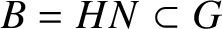 $B=HN\subset G$
is a Borel subgroup, H is a maximal torus and N is the unipotent radical of B. For each affine Weyl group element
$B=HN\subset G$
is a Borel subgroup, H is a maximal torus and N is the unipotent radical of B. For each affine Weyl group element
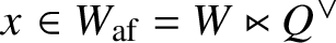 $x\in W_{\mathrm {af}} = W \ltimes Q^{\vee }$
, with
$x\in W_{\mathrm {af}} = W \ltimes Q^{\vee }$
, with
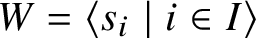 $W = \langle s_i \mid i \in I \rangle $
the (finite) Weyl group and
$W = \langle s_i \mid i \in I \rangle $
the (finite) Weyl group and
 $Q^{\vee } = \bigoplus _{i \in I} \mathbb {Z} \alpha _i^{\vee }$
the coroot lattice of G, one has a semi-infinite Schubert variety
$Q^{\vee } = \bigoplus _{i \in I} \mathbb {Z} \alpha _i^{\vee }$
the coroot lattice of G, one has a semi-infinite Schubert variety
 $\mathbf {Q}_{G}(x)\subset \mathbf {Q}_{G}^{\mathrm {rat}}$
, which is infinite-dimensional and is given as an orbit closure for the Iwahori subgroup
$\mathbf {Q}_{G}(x)\subset \mathbf {Q}_{G}^{\mathrm {rat}}$
, which is infinite-dimensional and is given as an orbit closure for the Iwahori subgroup
 $\mathbf {I}\subset G(\mathbb {C}[\![z]\!])$
. We distinguish the semi-infinite Schubert variety
$\mathbf {I}\subset G(\mathbb {C}[\![z]\!])$
. We distinguish the semi-infinite Schubert variety
 $\mathbf {Q}_{G} := \mathbf {Q}_{G}(e) \subset \mathbf {Q}_{G}^{\mathrm {rat}}$
associated to the identity element e of the affine Weyl group, and also call it the semi-infinite flag manifold.
$\mathbf {Q}_{G} := \mathbf {Q}_{G}(e) \subset \mathbf {Q}_{G}^{\mathrm {rat}}$
associated to the identity element e of the affine Weyl group, and also call it the semi-infinite flag manifold.
Our main object of study is the equivariant K-group
 $K_{H \times \mathbb {C}^{\ast }}(\mathbf {Q}_{G})$
–and that of
$K_{H \times \mathbb {C}^{\ast }}(\mathbf {Q}_{G})$
–and that of
 $\mathbf {Q}_{G}^{\mathrm {rat}}$
, denoted by
$\mathbf {Q}_{G}^{\mathrm {rat}}$
, denoted by
 $K_{H \times \mathbb {C}^{\ast }}\big(\mathbf {Q}_{G}^{\mathrm {rat}}\big )$
–which is a variant of the K-group
$K_{H \times \mathbb {C}^{\ast }}\big(\mathbf {Q}_{G}^{\mathrm {rat}}\big )$
–which is a variant of the K-group
 $K_{\tilde {\mathbf {I}}}^{\prime }(\mathbf {Q}_{G})$
introduced recently in [Reference Kato, Naito and Sagaki13]. Our K-group is a module over the equivariant scalar ring
$K_{\tilde {\mathbf {I}}}^{\prime }(\mathbf {Q}_{G})$
introduced recently in [Reference Kato, Naito and Sagaki13]. Our K-group is a module over the equivariant scalar ring
 $\mathbb {Z}\left [q^{\pm 1}\right ][P]$
, where P is the weight lattice of G,
$\mathbb {Z}\left [q^{\pm 1}\right ][P]$
, where P is the weight lattice of G,
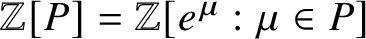 $\mathbb {Z}[P]=\mathbb {Z}[e^{\mu } : \mu \in P]$
is the character ring of H and
$\mathbb {Z}[P]=\mathbb {Z}[e^{\mu } : \mu \in P]$
is the character ring of H and
 $q\in R(\mathbb {C}^*)$
is the character of loop rotation. Therefore, the K-group
$q\in R(\mathbb {C}^*)$
is the character of loop rotation. Therefore, the K-group
 $K_{H \times \mathbb {C}^{\ast }}(\mathbf {Q}_{G})$
is a
$K_{H \times \mathbb {C}^{\ast }}(\mathbf {Q}_{G})$
is a
 $\mathbb {Z}\left [q^{\pm 1}\right ][P]$
-submodule of an extension of scalars of the equivariant K-group
$\mathbb {Z}\left [q^{\pm 1}\right ][P]$
-submodule of an extension of scalars of the equivariant K-group
 $K_{\tilde {\mathbf {I}}}^{\prime }(\mathbf {Q}_{G})$
of [Reference Kato, Naito and Sagaki13] with respect to the Iwahori subgroup
$K_{\tilde {\mathbf {I}}}^{\prime }(\mathbf {Q}_{G})$
of [Reference Kato, Naito and Sagaki13] with respect to the Iwahori subgroup
 $\mathbf {I}$
and loop rotation.
$\mathbf {I}$
and loop rotation.
A fundamental result of [Reference Kato, Naito and Sagaki13] is the combinatorial Chevalley formula for dominant weights in the K-group
 $K_{\tilde {\mathbf {I}}}^{\prime }(\mathbf {Q}_{G})$
(and hence in
$K_{\tilde {\mathbf {I}}}^{\prime }(\mathbf {Q}_{G})$
(and hence in
 $K_{H \times \mathbb {C}^{\ast }}(\mathbf {Q}_{G})$
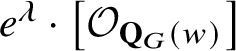
). This formula describes, in terms of semi-infinite Lakshmibai–Seshadri paths, the tensor product of the class of the line bundle
$K_{H \times \mathbb {C}^{\ast }}(\mathbf {Q}_{G})$
). This formula describes, in terms of semi-infinite Lakshmibai–Seshadri paths, the tensor product of the class of the line bundle
 $\left [\mathcal {O}_{\mathbf {Q}_{G}}(\lambda )\right ]$
associated to a dominant weight
$\left [\mathcal {O}_{\mathbf {Q}_{G}}(\lambda )\right ]$
associated to a dominant weight
 $\lambda \in P^+$
with the class of the structure sheaf
$\lambda \in P^+$
with the class of the structure sheaf
 $\left [\mathcal {O}_{\mathbf {Q}_{G}(x)}\right ]$
of a semi-infinite Schubert variety
$\left [\mathcal {O}_{\mathbf {Q}_{G}(x)}\right ]$
of a semi-infinite Schubert variety
 $\mathbf {Q}_{G}(x) \subset \mathbf {Q}_{G}$
for
$\mathbf {Q}_{G}(x) \subset \mathbf {Q}_{G}$
for
 $x = w t_{\xi } \in W_{\mathrm {af}}^{\geq 0} := W \times Q^{\vee ,+} \subset W_{\mathrm {af}}$
, where
$x = w t_{\xi } \in W_{\mathrm {af}}^{\geq 0} := W \times Q^{\vee ,+} \subset W_{\mathrm {af}}$
, where
 $Q^{\vee ,+} := \sum _{i \in I} \mathbb {Z}_{\geq 0} \alpha _{i}^{\vee } \subset Q^{\vee }$
. This was followed up in [Reference Naito, Orr and Sagaki24] by another combinatorial Chevalley formula in
$Q^{\vee ,+} := \sum _{i \in I} \mathbb {Z}_{\geq 0} \alpha _{i}^{\vee } \subset Q^{\vee }$
. This was followed up in [Reference Naito, Orr and Sagaki24] by another combinatorial Chevalley formula in
 $K_{H\times \mathbb {C}^*}(\mathbf {Q}_{G})$
, giving the tensor product of a Schubert class with an antidominant line bundle. The two Chevalley formulas–dominant [Reference Kato, Naito and Sagaki13] and antidominant [Reference Naito, Orr and Sagaki24]–were unified in [Reference Lenart, Naito and Sagaki19], giving the general Chevalley formula in
$K_{H\times \mathbb {C}^*}(\mathbf {Q}_{G})$
, giving the tensor product of a Schubert class with an antidominant line bundle. The two Chevalley formulas–dominant [Reference Kato, Naito and Sagaki13] and antidominant [Reference Naito, Orr and Sagaki24]–were unified in [Reference Lenart, Naito and Sagaki19], giving the general Chevalley formula in
 $K_{H\times \mathbb {C}^*}(\mathbf {Q}_{G})$
for arbitrary weights
$K_{H\times \mathbb {C}^*}(\mathbf {Q}_{G})$
for arbitrary weights
 $\lambda \in P$
.
$\lambda \in P$
.
The Chevalley formulas of [Reference Kato, Naito and Sagaki13, Reference Naito, Orr and Sagaki24, Reference Lenart, Naito and Sagaki19] thus provide the complete analogue for semi-infinite flag manifolds of their previously well-understood K-theory counterparts for the standard Kac–Moody flag varieties [Reference Pittie and Ram26, Reference Littelmann and Seshadri22, Reference Griffeth and Ram7, Reference Lenart and Postnikov20, Reference Lenart and Shimozono21]. In all such formulas, the objective is to expand the tensor product of a Schubert class with an equivariant line bundle, as a linear combination of Schubert classes with equivariant scalar coefficients. In the case of
 $\mathbf {Q}_{G}$
, by [Reference Lenart, Naito and Sagaki19], this takes the form
$\mathbf {Q}_{G}$
, by [Reference Lenart, Naito and Sagaki19], this takes the form
 $$ \begin{align} \left[\mathcal{O}_{\mathbf{Q}_{G}(x)}(\lambda)\right] = \sum_{\substack{y\in W_{\mathrm{af}}^{\ge 0}\\\mu\in P}} c_{x,y}^{\lambda,\mu} \cdot e^\mu \cdot \left[\mathcal{O}_{\mathbf{Q}_{G}(y)}\right], \end{align} $$
with
 $x,y\in W_{\mathrm {af}}^{\ge 0}$
,
$x,y\in W_{\mathrm {af}}^{\ge 0}$
,
 $\lambda ,\mu \in P$
and
$\lambda ,\mu \in P$
and
 $c_{x,y}^{\lambda ,\mu }\in \mathbb {Z}\left [q^{\pm 1}\right ]$
. We note that the sum on the right-hand side of equation (1.1), while generally infinite, satisfies a notion of convergence introduced in [Reference Kato, Naito and Sagaki13].
$c_{x,y}^{\lambda ,\mu }\in \mathbb {Z}\left [q^{\pm 1}\right ]$
. We note that the sum on the right-hand side of equation (1.1), while generally infinite, satisfies a notion of convergence introduced in [Reference Kato, Naito and Sagaki13].
In this paper, we shall study the inverseFootnote
1
expansion in
 $K_{H\times \mathbb {C}^*}(\mathbf {Q}_{G})$
:
$K_{H\times \mathbb {C}^*}(\mathbf {Q}_{G})$
:
 $$ \begin{align} e^\lambda\cdot \left[\mathcal{O}_{\mathbf{Q}_{G}(x)}\right] &= \sum_{\substack{y\in W_{\mathrm{af}}^{\ge 0}\\\mu\in P}} d_{x,y}^{\lambda,\mu}\cdot \left[\mathcal{O}_{\mathbf{Q}_{G}(y)}(\mu)\right] \end{align} $$
for
 $x\in W_{\mathrm {af}}^{\ge 0}$
and
$x\in W_{\mathrm {af}}^{\ge 0}$
and
 $\lambda \in P$
. In contrast to equation (1.1), the expansion in equation (1.2) is finite, as established in [Reference Orr25] for simply laced G–namely,
$\lambda \in P$
. In contrast to equation (1.1), the expansion in equation (1.2) is finite, as established in [Reference Orr25] for simply laced G–namely,
 $d_{x,y}^{\lambda ,\mu }\in \mathbb {Z}\left [q^{\pm 1}\right ]$
for any
$d_{x,y}^{\lambda ,\mu }\in \mathbb {Z}\left [q^{\pm 1}\right ]$
for any
 $\lambda ,\mu \in P$
and
$\lambda ,\mu \in P$
and
 $x,y\in W_{\mathrm {af}}^{\ge 0}$
, and the right-hand side of equation (1.2) is always a finite sum. (These properties are expected to hold for arbitrary G.)
$x,y\in W_{\mathrm {af}}^{\ge 0}$
, and the right-hand side of equation (1.2) is always a finite sum. (These properties are expected to hold for arbitrary G.)
We call any formula for the right-hand side of equation (1.2) an inverse Chevalley formula for
 $\lambda \in P$
in
$\lambda \in P$
in
 $K_{H\times \mathbb {C}^*}(\mathbf {Q}_{G})$
. The analogous expansion for finite-dimensional flag manifolds
$K_{H\times \mathbb {C}^*}(\mathbf {Q}_{G})$
. The analogous expansion for finite-dimensional flag manifolds
 $G/B$
was studied by Mathieu [Reference Mathieu23] in the context of filtrations of B-modules (compare [Reference Mathieu23, p. 239]). In fact, by [Reference Kato10, Proof of Proposition 1.15], one has a surjective map of
$G/B$
was studied by Mathieu [Reference Mathieu23] in the context of filtrations of B-modules (compare [Reference Mathieu23, p. 239]). In fact, by [Reference Kato10, Proof of Proposition 1.15], one has a surjective map of
 $\mathbb {Z}[P]$
-modules given by
$\mathbb {Z}[P]$
-modules given by
 $$ \begin{align} K_{H\times\mathbb{C}^*}(\mathbf{Q}_{G}) &\overset{\mathrm{trunc}}{\longrightarrow} K_H(G/B)\notag\\ q &\longmapsto 1\notag\\ \left[\mathcal{O}_{\mathbf{Q}_{G}(y)}\right] &\longmapsto \begin{cases}\left[\mathcal{O}_{X(y)}\right] &\text{if}\ y\in W,\\0 &\text{otherwise,}\end{cases} \end{align} $$
where
 $\left [\mathcal {O}_{X(y)}\right ]$
for
$\left [\mathcal {O}_{X(y)}\right ]$
for
 $y\in W$
denotes the structure sheaf of the Schubert variety
$y\in W$
denotes the structure sheaf of the Schubert variety
 $$ \begin{align} X(y)=\overline{Byw_{\circ} B/B}\subset G/B \end{align} $$
and
 $w_{\circ }$
is the longest element of W. The map
$w_{\circ }$
is the longest element of W. The map
 $\mathrm {trunc}$
also respects the tensor product by equivariant line bundles. Thus, for
$\mathrm {trunc}$
also respects the tensor product by equivariant line bundles. Thus, for
 $x\in W$
, the image of equation (1.2) under
$x\in W$
, the image of equation (1.2) under
 $\mathrm {trunc}$
produces the analogous inverse Chevalley expansion in
$\mathrm {trunc}$
produces the analogous inverse Chevalley expansion in
 $K_H(G/B)$
(see also Remark 3.13). In this sense, any inverse Chevalley formula (1.2) must incorporate the necessary ‘corrections’ in
$K_H(G/B)$
(see also Remark 3.13). In this sense, any inverse Chevalley formula (1.2) must incorporate the necessary ‘corrections’ in
 $K_{H\times \mathbb {C}^*}(\mathbf {Q}_{G})$
to the classical inverse Chevalley formulas in
$K_{H\times \mathbb {C}^*}(\mathbf {Q}_{G})$
to the classical inverse Chevalley formulas in
 $K_H(G/B)$
.
$K_H(G/B)$
.
We note that in the case of
 $K_H(G/B)$
, there is a simple transformation to pass between ordinary and inverse Chevalley formulas (as explained in, e.g., [Reference Mathieu23, p. 239]). The lack of such a transformation for
$K_H(G/B)$
, there is a simple transformation to pass between ordinary and inverse Chevalley formulas (as explained in, e.g., [Reference Mathieu23, p. 239]). The lack of such a transformation for
 $K_{H\times \mathbb {C}^*}(\mathbf {Q}_{G})$
justifies the independent study of inverse Chevalley formulas in the semi-infinite setting. Moreover, the finiteness of equation (1.2) offers an advantage over equation (1.1).
$K_{H\times \mathbb {C}^*}(\mathbf {Q}_{G})$
justifies the independent study of inverse Chevalley formulas in the semi-infinite setting. Moreover, the finiteness of equation (1.2) offers an advantage over equation (1.1).
The purpose of this paper is to prove a completely explicit, combinatorial inverse Chevalley formula in the equivariant K-group
 $K_{H \times \mathbb {C}^*}(\mathbf {Q}_{G})$
in the case of a simply laced group G and a minuscule weight
$K_{H \times \mathbb {C}^*}(\mathbf {Q}_{G})$
in the case of a simply laced group G and a minuscule weight
 $\lambda \in P$
. Before stating our results more precisely, let us discuss further motivations for this work.
$\lambda \in P$
. Before stating our results more precisely, let us discuss further motivations for this work.
1.1. Nil-DAHA and q-Heisenberg actions on
 $K_{H \times \mathbb {C}^*}\big(\mathbf {Q}_{G}^{\mathrm {rat}}\big )$

One approach to understanding equations (1.1) and (1.2) is that they relate two actions of the group algebra
 $\mathbb {Z}[P]$
on
$\mathbb {Z}[P]$
on
 $K_{H \times \mathbb {C}^*}\big(\mathbf {Q}_{G}^{\mathrm {rat}}\big )$
, one given by equivariant scalar multiplication (the left-hand side of equation (1.2)) and the other by the tensor product with equivariant line bundles (the left-hand side of equation (1.1)). These actions of
$K_{H \times \mathbb {C}^*}\big(\mathbf {Q}_{G}^{\mathrm {rat}}\big )$
, one given by equivariant scalar multiplication (the left-hand side of equation (1.2)) and the other by the tensor product with equivariant line bundles (the left-hand side of equation (1.1)). These actions of
 $\mathbb {Z}[P]$
extend to that of two distinct algebras on
$\mathbb {Z}[P]$
extend to that of two distinct algebras on
 $K_{H \times \mathbb {C}^*}\big(\mathbf {Q}_{G}^{\mathrm {rat}}\big )$
: the nil double affine Hecke algebra (nil-DAHA) and a q-Heisenberg algebra.
$K_{H \times \mathbb {C}^*}\big(\mathbf {Q}_{G}^{\mathrm {rat}}\big )$
: the nil double affine Hecke algebra (nil-DAHA) and a q-Heisenberg algebra.
Multiplication by equivariant scalars extends to a left action of the nil-DAHA
 $\mathbb {H}_0$
on
$\mathbb {H}_0$
on
 $K_{H \times \mathbb {C}^*}\big(\mathbf {Q}_{G}^{\mathrm {rat}}\big )$
, in a way that is conceptually similar to the action of nil-Hecke algebras on the equivariant K-theory of Kac–Moody flag varieties [Reference Kostant and Kumar8]. On the right, however, instead of a nil-Hecke algebra, one has an action of a q-Heisenberg algebra
$K_{H \times \mathbb {C}^*}\big(\mathbf {Q}_{G}^{\mathrm {rat}}\big )$
, in a way that is conceptually similar to the action of nil-Hecke algebras on the equivariant K-theory of Kac–Moody flag varieties [Reference Kostant and Kumar8]. On the right, however, instead of a nil-Hecke algebra, one has an action of a q-Heisenberg algebra
 $\mathfrak {H}$
. This is generated by tensor products with equivariant line bundles
$\mathfrak {H}$
. This is generated by tensor products with equivariant line bundles
 $[\mathcal {O}(\lambda )]$
(
$[\mathcal {O}(\lambda )]$
(
 $\lambda \in P$
) and translations
$\lambda \in P$
) and translations
 $Q^\vee \cong H(\mathbb {C}\left (\!\left (z\right )\!\right ))/H(\mathbb {C}[\![z]\!])$
. The two actions commute, making
$Q^\vee \cong H(\mathbb {C}\left (\!\left (z\right )\!\right ))/H(\mathbb {C}[\![z]\!])$
. The two actions commute, making
 $K_{H \times \mathbb {C}^*}\big(\mathbf {Q}_{G}^{\mathrm {rat}}\big )$
an
$K_{H \times \mathbb {C}^*}\big(\mathbf {Q}_{G}^{\mathrm {rat}}\big )$
an
 $(\mathbb {H}_0,\mathfrak {H})$
-bimodule.
$(\mathbb {H}_0,\mathfrak {H})$
-bimodule.
This bimodule structure is a fundamental tool in the study of
 $K_{H \times \mathbb {C}^*}\big(\mathbf {Q}_{G}^{\mathrm {rat}}\big )$
, as standard methods such as localisation are not available. Furthermore, as explained in [Reference Orr25], it gives a geometric realisation of the nonsymmetric q-Toda system introduced in [Reference Cherednik and Orr4] (see [Reference Braverman and Finkelberg1, Reference Braverman and Finkelberg2, Reference Givental and Lee5] for related results on the usual q-Toda system and [Reference Koroteev14, Reference Koroteev and Zeitlin15] for its
$K_{H \times \mathbb {C}^*}\big(\mathbf {Q}_{G}^{\mathrm {rat}}\big )$
, as standard methods such as localisation are not available. Furthermore, as explained in [Reference Orr25], it gives a geometric realisation of the nonsymmetric q-Toda system introduced in [Reference Cherednik and Orr4] (see [Reference Braverman and Finkelberg1, Reference Braverman and Finkelberg2, Reference Givental and Lee5] for related results on the usual q-Toda system and [Reference Koroteev14, Reference Koroteev and Zeitlin15] for its
 $(\mathsf {q},\mathsf {t})$
-extension given by Macdonald difference operators in type A). For us, the fact that the
$(\mathsf {q},\mathsf {t})$
-extension given by Macdonald difference operators in type A). For us, the fact that the
 $\mathbb {H}_0$
-action on
$\mathbb {H}_0$
-action on
 $K_{H \times \mathbb {C}^*}\big(\mathbf {Q}_{G}^{\mathrm {rat}}\big )$
includes the operators of multiplication by equivariant scalars is key. We use the limit construction [Reference Orr25] of the
$K_{H \times \mathbb {C}^*}\big(\mathbf {Q}_{G}^{\mathrm {rat}}\big )$
includes the operators of multiplication by equivariant scalars is key. We use the limit construction [Reference Orr25] of the
 $\mathbb {H}_0$
-action on
$\mathbb {H}_0$
-action on
 $K_{H \times \mathbb {C}^*}\big(\mathbf {Q}_{G}^{\mathrm {rat}}\big )$
to find and prove our inverse Chevalley formula in
$K_{H \times \mathbb {C}^*}\big(\mathbf {Q}_{G}^{\mathrm {rat}}\big )$
to find and prove our inverse Chevalley formula in
 $K_{H\times \mathbb {C}^*}(\mathbf {Q}_{G})$
, which is given by Theorem 1.
$K_{H\times \mathbb {C}^*}(\mathbf {Q}_{G})$
, which is given by Theorem 1.
1.2. Quantum K-theory of
$G/B$

In [Reference Kato10, Reference Kato12], Kato established a
 $\mathbb {Z}[P]$
-module isomorphism – with
$\mathbb {Z}[P]$
-module isomorphism – with
 $\mathbb {Z}[P]$
acting by equivariant scalars – from the (completed) H-equivariant quantum K-group
$\mathbb {Z}[P]$
acting by equivariant scalars – from the (completed) H-equivariant quantum K-group
 $QK_{H}(G/B) := K_{H}(G/B) \otimes \mathbb {Z}\left [\!\left [Q^{\vee ,+}\right ]\!\right ]$
of the finite-dimensional flag manifold
$QK_{H}(G/B) := K_{H}(G/B) \otimes \mathbb {Z}\left [\!\left [Q^{\vee ,+}\right ]\!\right ]$
of the finite-dimensional flag manifold
 $G/B$
onto the H-equivariant K-group
$G/B$
onto the H-equivariant K-group
 $K_{H}(\mathbf {Q}_{G})$
obtained by specialising
$K_{H}(\mathbf {Q}_{G})$
obtained by specialising
 $q=1$
in
$q=1$
in
 $K_{H\times \mathbb {C}^*}(\mathbf {Q}_{G})$
. (Here
$K_{H\times \mathbb {C}^*}(\mathbf {Q}_{G})$
. (Here
 $\mathbb {Z}\left [\!\left [Q^{\vee ,+}\right ]\!\right ]$
is the ring of formal power series in the (Novikov) variables
$\mathbb {Z}\left [\!\left [Q^{\vee ,+}\right ]\!\right ]$
is the ring of formal power series in the (Novikov) variables
 $Q_{i}$
,
$Q_{i}$
,
 $i \in I$
.) Kato’s isomorphism respects Schubert classes and intertwines the quantum multiplication in
$i \in I$
.) Kato’s isomorphism respects Schubert classes and intertwines the quantum multiplication in
 $QK_{H}(G/B)$
with the tensor product by line bundles in
$QK_{H}(G/B)$
with the tensor product by line bundles in
 $K_H(\mathbf {Q}_{G})$
. Thus it provides a means to transport formulas from
$K_H(\mathbf {Q}_{G})$
. Thus it provides a means to transport formulas from
 $K_H(\mathbf {Q}_{G})$
to
$K_H(\mathbf {Q}_{G})$
to
 $QK_H(G/B)$
. In the sequel [Reference Kouno, Naito, Orr and Sagaki16] to this paper, we will use Kato’s isomorphism to derive a corresponding inverse Chevalley formula in
$QK_H(G/B)$
. In the sequel [Reference Kouno, Naito, Orr and Sagaki16] to this paper, we will use Kato’s isomorphism to derive a corresponding inverse Chevalley formula in
 $QK_{H}(G/B)$
.
$QK_{H}(G/B)$
.
1.3. Our results
Let us now explain our results in more detail. Recall that a weight
 $\lambda \in P$
is called minuscule if
$\lambda \in P$
is called minuscule if
 $\left \langle \lambda ,\alpha ^\vee \right \rangle \in \{0,\pm 1\}$
for all
$\left \langle \lambda ,\alpha ^\vee \right \rangle \in \{0,\pm 1\}$
for all
 $\alpha \in \Delta $
. Nonzero minuscule weights exist in all types except
$\alpha \in \Delta $
. Nonzero minuscule weights exist in all types except
 $E_8$
,
$E_8$
,
 $F_4$
and
$F_4$
and
 $G_2$
.
$G_2$
.
Our results explicitly describe the inverse Chevalley formula in
 $K_{H\times \mathbb {C}^*}(\mathbf {Q}_{G})$
for arbitrary minuscule weights
$K_{H\times \mathbb {C}^*}(\mathbf {Q}_{G})$
for arbitrary minuscule weights
 $\lambda \in P$
in the case when G is simply laced. By iteration, our formulas completely determine the inverse Chevalley rule for arbitrary weights in ADE type (except in type
$\lambda \in P$
in the case when G is simply laced. By iteration, our formulas completely determine the inverse Chevalley rule for arbitrary weights in ADE type (except in type
 $E_8$
). Indeed, a result of Stembridge [Reference Stembridge27] (as stated in [Reference Lenart18, Theorem 2.1]) asserts that in all types except
$E_8$
). Indeed, a result of Stembridge [Reference Stembridge27] (as stated in [Reference Lenart18, Theorem 2.1]) asserts that in all types except
 $E_8$
,
$E_8$
,
 $F_4$
and
$F_4$
and
 $G_2$
, the minuscule weights form a set of generators for the weight lattice. (The full version of Stembridge’s result, which holds in arbitrary type, requires quasi-minuscule weights. We plan to take up the study of our constructions in the case of quasi-minuscule weights elsewhere.)
$G_2$
, the minuscule weights form a set of generators for the weight lattice. (The full version of Stembridge’s result, which holds in arbitrary type, requires quasi-minuscule weights. We plan to take up the study of our constructions in the case of quasi-minuscule weights elsewhere.)
Any minuscule weight belongs to the Weyl group orbit of a dominant minuscule weight – that is, a minuscule fundamental weight. Suppose
 $\varpi _k\in P^+$
is a minuscule fundamental weight. Set
$\varpi _k\in P^+$
is a minuscule fundamental weight. Set
 $J=I\setminus \{k\}$
, and consider the parabolic subgroup
$J=I\setminus \{k\}$
, and consider the parabolic subgroup
 $W_J=\left \langle s_j \mid j\in J\right \rangle $
, which is the stabiliser of
$W_J=\left \langle s_j \mid j\in J\right \rangle $
, which is the stabiliser of
 $\varpi _k$
. Let
$\varpi _k$
. Let
 $W^J$
be the set of minimal coset representatives for
$W^J$
be the set of minimal coset representatives for
 $W/W_J$
. Finally, let
$W/W_J$
. Finally, let
 $\lambda =x\varpi _k\in P$
be an arbitrary minuscule weight, where
$\lambda =x\varpi _k\in P$
be an arbitrary minuscule weight, where
 $x\in W^J$
.
$x\in W^J$
.
1.3.1. Algebraic formula
For G simply laced,
 $\lambda $
as before and any
$\lambda $
as before and any
 $w\in W$
, our first main result gives an algebraic expression for the product
$w\in W$
, our first main result gives an algebraic expression for the product
 $e^\lambda \cdot \left [\mathcal {O}_{\mathbf {Q}_{G}(w)}\right ]\in K_{H\times \mathbb {C}^*}(\mathbf {Q}_{G})$
in terms of the right q-Heisenberg action on
$e^\lambda \cdot \left [\mathcal {O}_{\mathbf {Q}_{G}(w)}\right ]\in K_{H\times \mathbb {C}^*}(\mathbf {Q}_{G})$
in terms of the right q-Heisenberg action on
 $K_{H\times \mathbb {C}^*}\big(\mathbf {Q}_{G}^{\mathrm {rat}}\big )$
. This is given explicitly as a sum over a set
$K_{H\times \mathbb {C}^*}\big(\mathbf {Q}_{G}^{\mathrm {rat}}\big )$
. This is given explicitly as a sum over a set
 $\mathbf {QW}_{\lambda ,w}$
of walks
$\mathbf {QW}_{\lambda ,w}$
of walks
 $(w_1,\dotsc ,w_n)$
in the quantum Bruhat graph
$(w_1,\dotsc ,w_n)$
in the quantum Bruhat graph
 $\mathrm {QBG}(W)$
[Reference Brenti, Fomin and Postnikov3], beginning at
$\mathrm {QBG}(W)$
[Reference Brenti, Fomin and Postnikov3], beginning at
 $w_0=w$
and with steps prescribed by a set of positive roots determined by
$w_0=w$
and with steps prescribed by a set of positive roots determined by
 $\lambda $
. (Here n is the length of the minimal representative of the coset
$\lambda $
. (Here n is the length of the minimal representative of the coset
 $w_{\circ } W_J$
.)
$w_{\circ } W_J$
.)
Theorem 1 (= Theorem 3.11)
Assume that G is of
 $ADE$
type but not of type
$ADE$
type but not of type
 $E_8$
. For any minuscule weight
$E_8$
. For any minuscule weight
 $\lambda =x\varpi _k\in P$
, where
$\lambda =x\varpi _k\in P$
, where
 $x\in W^J$
, and any
$x\in W^J$
, and any
 $w\in W$
, we have
$w\in W$
, we have
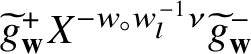
 $$ \begin{align} e^\lambda\cdot\left[\mathcal{O}_{\mathbf{Q}_{G}(w)}\right] = \sum_{\mathbf{w}=(w_1,\dotsc,w_n)\in\mathbf{QW}_{\lambda,w}}\left[\mathcal{O}_{\mathbf{Q}_{G}(w_n)}\right]\cdot \widetilde{g}^+_{\mathbf{w}} X^{-w_{\circ} w_l^{-1}\lambda} \widetilde{g}^-_{\mathbf{w}}, \end{align} $$
where
 $l=\ell (x)$
and
$l=\ell (x)$
and
 $\widetilde {g}^+_{\mathbf {w}} X^{-w_{\circ } w_l^{-1}\nu } \widetilde {g}^-_{\mathbf {w}}$
is an element of the q-Heisenberg algebra
$\widetilde {g}^+_{\mathbf {w}} X^{-w_{\circ } w_l^{-1}\nu } \widetilde {g}^-_{\mathbf {w}}$
is an element of the q-Heisenberg algebra
 $\mathfrak {H}$
given explicitly by equations (3.63) and (3.64).
$\mathfrak {H}$
given explicitly by equations (3.63) and (3.64).
Acting by translations from the q-Heisenberg algebra, one immediately obtains a corresponding formula for
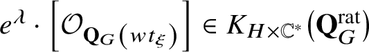 $e^\lambda \cdot \left [\mathcal {O}_{\mathbf {Q}_{G}\left (wt_\xi \right )}\right ]\in K_{H\times \mathbb {C}^*}\big(\mathbf {Q}_{G}^{\mathrm {rat}}\big )$
, for any
$e^\lambda \cdot \left [\mathcal {O}_{\mathbf {Q}_{G}\left (wt_\xi \right )}\right ]\in K_{H\times \mathbb {C}^*}\big(\mathbf {Q}_{G}^{\mathrm {rat}}\big )$
, for any
 $\xi \in Q^\vee $
.
$\xi \in Q^\vee $
.
In order to prove Theorem 1, we apply the main result of [Reference Orr25]. The main step in our proof (see Theorem 3.7) is the intricate computation of a limit, as
 $\mathsf {t}\to 0$
, from the polynomial representation of the double affine Hecke algebra (DAHA). Thus one should also regard Theorem 1 as an explicit determination of all nonsymmetric q-Toda operators, in the sense of [Reference Cherednik and Orr4, Reference Orr25], for minuscule weights in ADE type.
$\mathsf {t}\to 0$
, from the polynomial representation of the double affine Hecke algebra (DAHA). Thus one should also regard Theorem 1 as an explicit determination of all nonsymmetric q-Toda operators, in the sense of [Reference Cherednik and Orr4, Reference Orr25], for minuscule weights in ADE type.
1.3.2. Combinatorial formula
Our second main result expresses the same product
 $e^\lambda \cdot \left [\mathcal {O}_{\mathbf {Q}_{G}(w)}\right ]$
combinatorially. To achieve this, we enhance the set of quantum walks
$e^\lambda \cdot \left [\mathcal {O}_{\mathbf {Q}_{G}(w)}\right ]$
combinatorially. To achieve this, we enhance the set of quantum walks
 $\mathbf {QW}_{\lambda ,w}$
to a set
$\mathbf {QW}_{\lambda ,w}$
to a set
 $\widetilde {\mathbf {QW}}_{\lambda ,w}$
of decorated quantum walks. Roughly speaking, a decorated quantum walk
$\widetilde {\mathbf {QW}}_{\lambda ,w}$
of decorated quantum walks. Roughly speaking, a decorated quantum walk
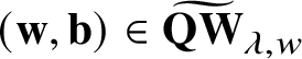 $(\mathbf {w},\mathbf {b})\in \widetilde {\mathbf {QW}}_{\lambda ,w}$
consists of a quantum walk
$(\mathbf {w},\mathbf {b})\in \widetilde {\mathbf {QW}}_{\lambda ,w}$
consists of a quantum walk
 $\mathbf {w}=(w_1,\dotsc ,w_n)\in \mathbf {QW}_{\lambda ,w}$
together with a decoration
$\mathbf {w}=(w_1,\dotsc ,w_n)\in \mathbf {QW}_{\lambda ,w}$
together with a decoration
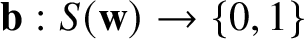 $\mathbf {b}: S(\mathbf {w})\to \{0,1\}$
. The latter is a
$\mathbf {b}: S(\mathbf {w})\to \{0,1\}$
. The latter is a
 $\{0,1\}$
-valued function on an explicit subset
$\{0,1\}$
-valued function on an explicit subset
 $S(\mathbf {w})\subset \{t : w_t=w_{t-1}\}$
of the stationary steps in the walk
$S(\mathbf {w})\subset \{t : w_t=w_{t-1}\}$
of the stationary steps in the walk
 $\mathbf {w}$
. Each
$\mathbf {w}$
. Each
 $(\mathbf {w},\mathbf {b})\in \widetilde {\mathbf {QW}}_{\lambda ,w}$
carries a sign
$(\mathbf {w},\mathbf {b})\in \widetilde {\mathbf {QW}}_{\lambda ,w}$
carries a sign
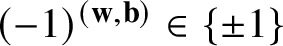 $(-1)^{(\mathbf {w},\mathbf {b})}\in \{\pm 1\}$
, a weight
$(-1)^{(\mathbf {w},\mathbf {b})}\in \{\pm 1\}$
, a weight
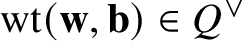 $\mathrm {wt}(\mathbf {w},\mathbf {b})\in Q^\vee $
and a degree
$\mathrm {wt}(\mathbf {w},\mathbf {b})\in Q^\vee $
and a degree
 $\deg (\mathbf {w},\mathbf {b})\in \mathbb {Z}$
. For details, see Section 3.4.1.
$\deg (\mathbf {w},\mathbf {b})\in \mathbb {Z}$
. For details, see Section 3.4.1.
Our combinatorial inverse Chevalley formula reads as follows:
Theorem 2 (= Theorem 3.14)
Assume that G is of
 $ADE$
type but not of type
$ADE$
type but not of type
 $E_8$
. For any minuscule weight
$E_8$
. For any minuscule weight
 $\lambda =x\varpi _k\in P$
, where
$\lambda =x\varpi _k\in P$
, where
 $x\in W^J$
, and any
$x\in W^J$
, and any
 $w\in W$
, we have
$w\in W$
, we have
 $$ \begin{align} &e^{\lambda}\cdot \left[\mathcal{O}_{\mathbf{Q}_{G}(w)}\right]\nonumber\\ &= \sum_{(\mathbf{w},\mathbf{b})\in\widetilde{\mathbf{QW}}_{\lambda,w}}(-1)^{(\mathbf{w},\mathbf{b})}q^{\deg(\mathbf{w},\mathbf{b})}\cdot[\mathcal{O}_{\mathbf{Q}_{G}(w_nt_{-w_\circ(\mathrm{wt}(\mathbf{w},\mathbf{b}))})}(-w_\circ w_l^{-1}\lambda+\mathrm{wt}(\mathbf{w},\mathbf{b}))]. \end{align} $$
Theorem 2 is obtained as an immediate consequence of Theorem 1, by fully expanding the right-hand side of equation (1.5) in the q-Heisenberg algebra. Our combinatorial framework is designed to record the terms in this expansion. We find it satisfying that the DAHA-based limit used to prove equation (1.5) automatically manufactures the combinatorics of decorated quantum walks necessary for both formulas. We mention that equation (1.5) gives the extension to
 $K_{H\times \mathbb {C}^*}(\mathbf {Q}_{G})$
of Lenart’s rule [Reference Lenart17, Theorem 3.1], which holds in
$K_{H\times \mathbb {C}^*}(\mathbf {Q}_{G})$
of Lenart’s rule [Reference Lenart17, Theorem 3.1], which holds in
 $K(SL(n+1)/B)$
, for multiplying a Grothendieck polynomial by a variable.
$K(SL(n+1)/B)$
, for multiplying a Grothendieck polynomial by a variable.
In Appendix A we work out some further details in the type A case, including concrete examples of equation (1.5) in equations (A.1) and (A.2) and the important special case
 $w=w_\circ $
,
$w=w_\circ $
,
 $k=1$
in equation (A.7). We also explain, following [Reference Orr25, §5.1], how to obtain the usual q-Toda difference operator by symmetrising Theorem 1.
$k=1$
in equation (A.7). We also explain, following [Reference Orr25, §5.1], how to obtain the usual q-Toda difference operator by symmetrising Theorem 1.
1.4. The sequel
In [Reference Kouno, Naito, Orr and Sagaki16] we will establish a different, equivalent version of our inverse Chevalley formula (1.6) in terms of paths (instead of walks) in the quantum Bruhat graph. By means of this alternate formula, we will give a separate and logically independent proof of Theorem 2 in type A, based on the Chevalley formulas of [Reference Kato, Naito and Sagaki13, Reference Naito, Orr and Sagaki24] and an equivalent set of character identities for Demazure submodules of level
 $0$
extremal weight modules. Finally, we will use Theorem 2 to derive a corresponding inverse Chevalley formula in the quantum K-ring
$0$
extremal weight modules. Finally, we will use Theorem 2 to derive a corresponding inverse Chevalley formula in the quantum K-ring
 $QK_H(G/B)$
, by means of Kato’s isomorphism.
$QK_H(G/B)$
, by means of Kato’s isomorphism.
2. Basic notation
2.1. Root system
Let G be a simply connected simple algebraic group over
 $\mathbb {C}$
. As in the introduction, we fix a maximal torus and Borel subgroup
$\mathbb {C}$
. As in the introduction, we fix a maximal torus and Borel subgroup
 $H\subset B\subset G$
. Set
$H\subset B\subset G$
. Set
 $\mathfrak {g} := \mathrm {Lie}(G)$
and
$\mathfrak {g} := \mathrm {Lie}(G)$
and
 $\mathfrak {h} := \mathrm {Lie}(H)$
. We denote by
$\mathfrak {h} := \mathrm {Lie}(H)$
. We denote by
 $\left \langle \cdot , \cdot \right \rangle : \mathfrak {h}^{\ast } \times \mathfrak {h} \rightarrow \mathbb {C}$
the canonical pairing, where
$\left \langle \cdot , \cdot \right \rangle : \mathfrak {h}^{\ast } \times \mathfrak {h} \rightarrow \mathbb {C}$
the canonical pairing, where
 $\mathfrak {h}^{\ast } = \mathrm {Hom}_{\mathbb {C}}(\mathfrak {h}, \mathbb {C})$
.
$\mathfrak {h}^{\ast } = \mathrm {Hom}_{\mathbb {C}}(\mathfrak {h}, \mathbb {C})$
.
Let
 $\Delta \subset \mathfrak {h}^{\ast }$
be the root system of
$\Delta \subset \mathfrak {h}^{\ast }$
be the root system of
 $\mathfrak {g}$
,
$\mathfrak {g}$
,
 $\Delta ^{+} \subset \Delta $
the positive roots (with respect to B) and
$\Delta ^{+} \subset \Delta $
the positive roots (with respect to B) and
 $\{ \alpha _{i} \}_{i \in I} \subset \Delta ^{+}$
the set of simple roots. We denote by
$\{ \alpha _{i} \}_{i \in I} \subset \Delta ^{+}$
the set of simple roots. We denote by
 $\alpha ^{\vee } \in \mathfrak {h}$
the coroot corresponding to
$\alpha ^{\vee } \in \mathfrak {h}$
the coroot corresponding to
 $\alpha \in \Delta $
. Also, we denote by
$\alpha \in \Delta $
. Also, we denote by
 $\theta \in \Delta ^+$
the highest root of
$\theta \in \Delta ^+$
the highest root of
 $\Delta $
, and we set
$\Delta $
, and we set
 $\rho := (1/2) \sum _{\alpha \in \Delta ^{+}} \alpha $
. The root lattice Q and the coroot lattice
$\rho := (1/2) \sum _{\alpha \in \Delta ^{+}} \alpha $
. The root lattice Q and the coroot lattice
 $Q^{\vee }$
of
$Q^{\vee }$
of
 $\mathfrak {g}$
are
$\mathfrak {g}$
are
 $Q := \sum _{i \in I} \mathbb {Z} \alpha _{i}$
and
$Q := \sum _{i \in I} \mathbb {Z} \alpha _{i}$
and
 $Q^{\vee } := \sum _{i \in I} \mathbb {Z} \alpha _{i}^{\vee }$
.
$Q^{\vee } := \sum _{i \in I} \mathbb {Z} \alpha _{i}^{\vee }$
.
For
 $i \in I$
, let
$i \in I$
, let
 $\varpi _{i} \in \mathfrak {h}^{\ast }$
be the fundamental weight determined by
$\varpi _{i} \in \mathfrak {h}^{\ast }$
be the fundamental weight determined by
 $\left \langle \varpi _{i}, \alpha _{j}^{\vee } \right \rangle = \delta _{i, j}$
for all
$\left \langle \varpi _{i}, \alpha _{j}^{\vee } \right \rangle = \delta _{i, j}$
for all
 $j \in I$
, where
$j \in I$
, where
 $\delta _{i, j}$
denotes the Kronecker delta. The weight lattice P of
$\delta _{i, j}$
denotes the Kronecker delta. The weight lattice P of
 $\mathfrak {g}$
is defined by
$\mathfrak {g}$
is defined by
 $P := \sum _{i \in I} \mathbb {Z} \varpi _{i}$
. We denote by
$P := \sum _{i \in I} \mathbb {Z} \varpi _{i}$
. We denote by
 $\mathbb {Z}[P]$
the group algebra of P – that is, the associative algebra generated by formal elements
$\mathbb {Z}[P]$
the group algebra of P – that is, the associative algebra generated by formal elements
 $\left \{ e^{\lambda } \mid \lambda \in P\right \}$
, where the product is defined by
$\left \{ e^{\lambda } \mid \lambda \in P\right \}$
, where the product is defined by
 $e^{\lambda } e^{\mu } := e^{\lambda + \mu }$
for
$e^{\lambda } e^{\mu } := e^{\lambda + \mu }$
for
 $\lambda , \mu \in P$
.
$\lambda , \mu \in P$
.
A reflection
 $s_{\alpha } \in GL(\mathfrak {h}^{\ast })$
,
$s_{\alpha } \in GL(\mathfrak {h}^{\ast })$
,
 $\alpha \in \Delta $
, is defined by
$\alpha \in \Delta $
, is defined by
 $s_{\alpha }(\lambda ) := \lambda - \left \langle \lambda , \alpha ^{\vee } \right \rangle \alpha $
for
$s_{\alpha }(\lambda ) := \lambda - \left \langle \lambda , \alpha ^{\vee } \right \rangle \alpha $
for
 $\lambda \in \mathfrak {h}^{\ast }$
. We write
$\lambda \in \mathfrak {h}^{\ast }$
. We write
 $s_{i} := s_{\alpha _{i}}$
for
$s_{i} := s_{\alpha _{i}}$
for
 $i \in I$
. Then the Weyl group
$i \in I$
. Then the Weyl group
 $W := \langle s_{i} \mid i \in I \rangle $
of
$W := \langle s_{i} \mid i \in I \rangle $
of
 $\mathfrak {g}$
is the subgroup of
$\mathfrak {g}$
is the subgroup of
 $GL(\mathfrak {h}^{\ast })$
generated by
$GL(\mathfrak {h}^{\ast })$
generated by
 $\{ s_{i} \}_{i \in I}$
. We denote by
$\{ s_{i} \}_{i \in I}$
. We denote by
 $\ell (w)$
the length of
$\ell (w)$
the length of
 $w\in W$
with respect to
$w\in W$
with respect to
 $\{ s_{i} \}_{i \in I}$
.
$\{ s_{i} \}_{i \in I}$
.
2.2. Quantum Bruhat graph
The quantum Bruhat graph
 $\mathrm {QBG}(W)$
(compare [Reference Brenti, Fomin and Postnikov3, Definition 6.1]) is the
$\mathrm {QBG}(W)$
(compare [Reference Brenti, Fomin and Postnikov3, Definition 6.1]) is the
 $\Delta ^+$
-labelled directed graph whose vertices are the elements of W and whose edges are of the form
$\Delta ^+$
-labelled directed graph whose vertices are the elements of W and whose edges are of the form
 $x \xrightarrow {\alpha } y$
, with
$x \xrightarrow {\alpha } y$
, with
 $x, y \in W$
and
$x, y \in W$
and
 $\alpha \in \Delta ^+$
, such that
$\alpha \in \Delta ^+$
, such that
 $y = x s_{\alpha }$
and either of the following holds: (B)
$y = x s_{\alpha }$
and either of the following holds: (B)
 $\ell (y) = \ell (x) + 1$
or (Q)
$\ell (y) = \ell (x) + 1$
or (Q)
 $\ell (y) = \ell (x) - 2\left \langle \rho , \alpha ^\vee \right \rangle + 1$
. An edge satisfying (B) (resp., (Q)) is called a Bruhat edge (resp., a quantum edge).
$\ell (y) = \ell (x) - 2\left \langle \rho , \alpha ^\vee \right \rangle + 1$
. An edge satisfying (B) (resp., (Q)) is called a Bruhat edge (resp., a quantum edge).
2.3. Affine root system
Let
 $\mathfrak {g}_{\mathrm {af}} := \left (\mathfrak {g} \otimes \mathbb {C}\left [z, z^{-1}\right ]\right ) \oplus \mathbb {C} c \oplus \mathbb {C} d$
be the (untwisted) affine Lie algebra over
$\mathfrak {g}_{\mathrm {af}} := \left (\mathfrak {g} \otimes \mathbb {C}\left [z, z^{-1}\right ]\right ) \oplus \mathbb {C} c \oplus \mathbb {C} d$
be the (untwisted) affine Lie algebra over
 $\mathbb {C}$
associated to
$\mathbb {C}$
associated to
 $\mathfrak {g}$
, where c is the canonical central element and d is the degree operator. Then
$\mathfrak {g}$
, where c is the canonical central element and d is the degree operator. Then
 $\mathfrak {h}_{\mathrm {af}} := \mathfrak {h} \oplus \mathbb {C} c \oplus \mathbb {C} d$
is the Cartan subalgebra of
$\mathfrak {h}_{\mathrm {af}} := \mathfrak {h} \oplus \mathbb {C} c \oplus \mathbb {C} d$
is the Cartan subalgebra of
 $\mathfrak {g}_{\mathrm {af}}$
. We denote by
$\mathfrak {g}_{\mathrm {af}}$
. We denote by
 $\left \langle \cdot , \cdot \right \rangle : \mathfrak {h}_{\mathrm {af}}^{\ast } \times \mathfrak {h}_{\mathrm {af}} \rightarrow \mathbb {C}$
the canonical pairing. Regarding
$\left \langle \cdot , \cdot \right \rangle : \mathfrak {h}_{\mathrm {af}}^{\ast } \times \mathfrak {h}_{\mathrm {af}} \rightarrow \mathbb {C}$
the canonical pairing. Regarding
 $\lambda \in \mathfrak {h}^{\ast }$
as
$\lambda \in \mathfrak {h}^{\ast }$
as
 $\lambda \in \mathfrak {h}_{\mathrm {af}}^{\ast } = \mathrm {Hom}_{\mathbb {C}}(\mathfrak {h}_{\mathrm {af}}, \mathbb {C})$
by setting
$\lambda \in \mathfrak {h}_{\mathrm {af}}^{\ast } = \mathrm {Hom}_{\mathbb {C}}(\mathfrak {h}_{\mathrm {af}}, \mathbb {C})$
by setting
 $\left \langle \lambda , c \right \rangle = \left \langle \lambda , d \right \rangle = 0$
, we have
$\left \langle \lambda , c \right \rangle = \left \langle \lambda , d \right \rangle = 0$
, we have
 $\mathfrak {h}^{\ast } \subset \mathfrak {h}_{\mathrm {af}}^{\ast }$
. In this identification, we see that the canonical pairing
$\mathfrak {h}^{\ast } \subset \mathfrak {h}_{\mathrm {af}}^{\ast }$
. In this identification, we see that the canonical pairing
 $\left \langle \cdot , \cdot \right \rangle $
on
$\left \langle \cdot , \cdot \right \rangle $
on
 $\mathfrak {h}_{\mathrm {af}}^{\ast } \times \mathfrak {h}_{\mathrm {af}}$
extends that on
$\mathfrak {h}_{\mathrm {af}}^{\ast } \times \mathfrak {h}_{\mathrm {af}}$
extends that on
 $\mathfrak {h}^{\ast } \times \mathfrak {h}$
.
$\mathfrak {h}^{\ast } \times \mathfrak {h}$
.
Let us consider the root system of
 $\mathfrak {g}_{\mathrm {af}}$
. We define
$\mathfrak {g}_{\mathrm {af}}$
. We define
 $\delta $
to be the unique element of
$\delta $
to be the unique element of
 $\mathfrak {h}_{\mathrm {af}}^{\ast }$
which satisfies
$\mathfrak {h}_{\mathrm {af}}^{\ast }$
which satisfies
 $\left \langle \delta , h \right \rangle = 0$
for all
$\left \langle \delta , h \right \rangle = 0$
for all
 $h \in \mathfrak {h}$
,
$h \in \mathfrak {h}$
,
 $\left \langle \delta , c \right \rangle = 0$
and
$\left \langle \delta , c \right \rangle = 0$
and
 $\left \langle \delta , d \right \rangle = 1$
. We set
$\left \langle \delta , d \right \rangle = 1$
. We set
 $\alpha _{0} := -\theta + \delta \in \mathfrak {h}_{\mathrm {af}}^{\ast }$
. Then the root system
$\alpha _{0} := -\theta + \delta \in \mathfrak {h}_{\mathrm {af}}^{\ast }$
. Then the root system
 $\Delta _{\mathrm {af}}$
of
$\Delta _{\mathrm {af}}$
of
 $\mathfrak {g}_{\mathrm {af}}$
has simple roots
$\mathfrak {g}_{\mathrm {af}}$
has simple roots
 $\{ \alpha _{i} \}_{i \in I_{\mathrm {af}}}$
, where
$\{ \alpha _{i} \}_{i \in I_{\mathrm {af}}}$
, where
 $I_{\mathrm {af}} := I \sqcup \{ 0 \}$
.
$I_{\mathrm {af}} := I \sqcup \{ 0 \}$
.
For each
 $\alpha \in \Delta _{\mathrm {af}}$
, we have a reflection
$\alpha \in \Delta _{\mathrm {af}}$
, we have a reflection
 $s_{\alpha } \in GL(\mathfrak {h}_{\mathrm {af}})$
, defined as for
$s_{\alpha } \in GL(\mathfrak {h}_{\mathrm {af}})$
, defined as for
 $\mathfrak {g}$
. Note that for
$\mathfrak {g}$
. Note that for
 $\alpha \in \Delta \subset \Delta _{\mathrm {af}}$
, the restriction of a reflection
$\alpha \in \Delta \subset \Delta _{\mathrm {af}}$
, the restriction of a reflection
 $s_{\alpha }$
defined on
$s_{\alpha }$
defined on
 $\mathfrak {h}_{\mathrm {af}}$
to
$\mathfrak {h}_{\mathrm {af}}$
to
 $\mathfrak {h}$
coincides with a reflection
$\mathfrak {h}$
coincides with a reflection
 $s_{\alpha }$
defined on
$s_{\alpha }$
defined on
 $\mathfrak {h}$
. Set
$\mathfrak {h}$
. Set
 $s_{i} := s_{\alpha _{i}}$
for
$s_{i} := s_{\alpha _{i}}$
for
 $i \in I_{\mathrm {af}}$
. Then the Weyl group
$i \in I_{\mathrm {af}}$
. Then the Weyl group
 $W_{\mathrm {af}}$
of
$W_{\mathrm {af}}$
of
 $\mathfrak {g}_{\mathrm {af}}$
(called the affine Weyl group) is defined to be the subgroup of
$\mathfrak {g}_{\mathrm {af}}$
(called the affine Weyl group) is defined to be the subgroup of
 $GL(\mathfrak {h}_{\mathrm {af}})$
generated by
$GL(\mathfrak {h}_{\mathrm {af}})$
generated by
 $\{ s_{i} \}_{i \in I_{\mathrm {af}}}$
, namely
$\{ s_{i} \}_{i \in I_{\mathrm {af}}}$
, namely
 $W_{\mathrm {af}} = \langle s_{i} \mid i \in I_{\mathrm {af}} \rangle $
. In [Reference Kac9, §6.5], it is shown that
$W_{\mathrm {af}} = \langle s_{i} \mid i \in I_{\mathrm {af}} \rangle $
. In [Reference Kac9, §6.5], it is shown that
 $W_{\mathrm {af}} \simeq W \ltimes \left \{ t_{\alpha ^{\vee }} \mid \alpha ^{\vee } \in Q^{\vee } \right \} \simeq W \ltimes Q^{\vee }$
, where
$W_{\mathrm {af}} \simeq W \ltimes \left \{ t_{\alpha ^{\vee }} \mid \alpha ^{\vee } \in Q^{\vee } \right \} \simeq W \ltimes Q^{\vee }$
, where
 $t_{\alpha ^{\vee }}$
is the translation element corresponding to
$t_{\alpha ^{\vee }}$
is the translation element corresponding to
 $\alpha ^{\vee } \in Q^{\vee }$
.
$\alpha ^{\vee } \in Q^{\vee }$
.
2.4. Simply laced assumption
While the definitions we have given are completely general, we will in fact assume throughout that G is simply laced. As a result, we almost always identify
 $\mathfrak {h}^\ast $
with
$\mathfrak {h}^\ast $
with
 $\mathfrak {h}$
, roots with coroots and so on. We do this by means of the nondegenerate W-invariant symmetric bilinear form
$\mathfrak {h}$
, roots with coroots and so on. We do this by means of the nondegenerate W-invariant symmetric bilinear form
 $(\cdot ,\cdot ) : \mathfrak {h}^* \times \mathfrak {h}^* \to \mathbb {C}$
, normalised so that
$(\cdot ,\cdot ) : \mathfrak {h}^* \times \mathfrak {h}^* \to \mathbb {C}$
, normalised so that
 $(\alpha ,\alpha )=2$
for all
$(\alpha ,\alpha )=2$
for all
 $\alpha \in \Delta $
. We write
$\alpha \in \Delta $
. We write
 $\lvert \lambda \rvert ^2=(\lambda ,\lambda )$
for
$\lvert \lambda \rvert ^2=(\lambda ,\lambda )$
for
 $\lambda \in \mathfrak {h}^*$
.
$\lambda \in \mathfrak {h}^*$
.
2.5. Extended affine Weyl group
Let
 $W_{\mathrm {ex}}=W\ltimes P$
be the extended affine Weyl group, which we let act on
$W_{\mathrm {ex}}=W\ltimes P$
be the extended affine Weyl group, which we let act on
 $P\oplus \mathbb {Z}\frac {\delta }{e}$
by the level
$P\oplus \mathbb {Z}\frac {\delta }{e}$
by the level
 $0$
action
$0$
action
 $$ \begin{align} wt_\mu (\lambda)=w(\lambda)-(\mu,\lambda)\delta,\qquad wt_\mu(\delta)=\delta. \end{align} $$
Here we choose e to be the smallest positive integer such that
 $e\cdot (P,P)\subset \mathbb {Z}$
.
$e\cdot (P,P)\subset \mathbb {Z}$
.
We also define the group
 $\Pi =P/Q$
, which we realise as the subgroup of length
$\Pi =P/Q$
, which we realise as the subgroup of length
 $0$
elements in
$0$
elements in
 $W_{\mathrm {ex}}$
.
$W_{\mathrm {ex}}$
.
2.6. Parameters
Let us introduce a parameter
 $q^{1/e}$
such that
$q^{1/e}$
such that
 $\left (q^{1/e}\right )^e=q$
, where
$\left (q^{1/e}\right )^e=q$
, where
 $q\in R(\mathbb {C}^*)$
is the equivariant parameter corresponding to loop rotation on
$q\in R(\mathbb {C}^*)$
is the equivariant parameter corresponding to loop rotation on
 $\mathbf {Q}_{G}^{\mathrm {rat}}$
. We will also use a related, but distinct parameter
$\mathbf {Q}_{G}^{\mathrm {rat}}$
. We will also use a related, but distinct parameter
 $\mathsf {q}^{1/e}$
, as well as parameters
$\mathsf {q}^{1/e}$
, as well as parameters
 $\mathsf {t},\mathsf {v}$
such that
$\mathsf {t},\mathsf {v}$
such that
 $\mathsf {t}=\mathsf {v}^2$
. Our base field for DAHA constructions will be
$\mathsf {t}=\mathsf {v}^2$
. Our base field for DAHA constructions will be
 $\mathsf {K}=\mathbb {Q}\left (\mathsf {q}^{1/e},\mathsf {v}\right )$
.
$\mathsf {K}=\mathbb {Q}\left (\mathsf {q}^{1/e},\mathsf {v}\right )$
.
2.7. Matrices
For any ring R with
 $1$
, let
$1$
, let
 $\mathrm {Mat}_W(R)$
denote the R-algebra of
$\mathrm {Mat}_W(R)$
denote the R-algebra of
 $W\times W$
matrices with entries in R. Let
$W\times W$
matrices with entries in R. Let
 $\{e_w\}_{w\in W}$
be the standard basis of the free R-module
$\{e_w\}_{w\in W}$
be the standard basis of the free R-module
 $R^{\lvert W\rvert }$
. For
$R^{\lvert W\rvert }$
. For
 $A\in \mathrm {Mat}_W(R)$
, we denote by
$A\in \mathrm {Mat}_W(R)$
, we denote by
 $A_{w,\bullet }=\sum _{v\in W}A_{w,v}e_v$
the row of the matrix A indexed by
$A_{w,\bullet }=\sum _{v\in W}A_{w,v}e_v$
the row of the matrix A indexed by
 $w\in W$
.
$w\in W$
.
3. Inverse Chevalley formula via DAHA
In this section we use the methods of [Reference Orr25], based on the
 $(\mathbb {H}_0,\mathfrak {H})$
-bimodule structure of
$(\mathbb {H}_0,\mathfrak {H})$
-bimodule structure of
 $K_{H \times \mathbb {C}^*}\big(\mathbf {Q}_{G}^{\mathrm {rat}}\big )$
, to prove the inverse Chevalley formulas (1.5) and (1.6).
$K_{H \times \mathbb {C}^*}\big(\mathbf {Q}_{G}^{\mathrm {rat}}\big )$
, to prove the inverse Chevalley formulas (1.5) and (1.6).
3.1. K-groups
Let
 $K_{\tilde {\mathbf {I}}}\big(\mathbf {Q}_{G}^{\mathrm {rat}}\big )$
be the equivariant K-group of
$K_{\tilde {\mathbf {I}}}\big(\mathbf {Q}_{G}^{\mathrm {rat}}\big )$
be the equivariant K-group of
 $\mathbf {Q}_{G}^{\mathrm {rat}}$
introduced in [Reference Kato, Naito and Sagaki13, §6], where
$\mathbf {Q}_{G}^{\mathrm {rat}}$
introduced in [Reference Kato, Naito and Sagaki13, §6], where
 $\tilde {\mathbf {I}}=\mathbf {I}\rtimes \mathbb {C}^*$
is a semidirect product of the Iwahori subgroup
$\tilde {\mathbf {I}}=\mathbf {I}\rtimes \mathbb {C}^*$
is a semidirect product of the Iwahori subgroup
 $\mathbf {I}\subset G(\mathbb {C}[\![z]\!])$
and loop rotation
$\mathbf {I}\subset G(\mathbb {C}[\![z]\!])$
and loop rotation
 $\mathbb {C}^*$
. Correspondingly,
$\mathbb {C}^*$
. Correspondingly,
 $K_{\tilde {\mathbf {I}}}\big(\mathbf {Q}_{G}^{\mathrm {rat}}\big )$
is a module over
$K_{\tilde {\mathbf {I}}}\big(\mathbf {Q}_{G}^{\mathrm {rat}}\big )$
is a module over
 $\mathbb {Z}[P]\left (\!\left (q^{-1}\right )\!\right )$
, which acts by equivariant scalar multiplication.
$\mathbb {Z}[P]\left (\!\left (q^{-1}\right )\!\right )$
, which acts by equivariant scalar multiplication.
One has the following classes in
 $K_{\tilde {\mathbf {I}}}\big(\mathbf {Q}_{G}^{\mathrm {rat}}\big )$
, for each
$K_{\tilde {\mathbf {I}}}\big(\mathbf {Q}_{G}^{\mathrm {rat}}\big )$
, for each
 $x\in W_{\mathrm {af}}$
and
$x\in W_{\mathrm {af}}$
and
 $\lambda \in P$
:
$\lambda \in P$
:
-
• Schubert classes
$\left [\mathcal {O}_{\mathbf {Q}_{G}(x)}\right ]$
-
• Equivariant line bundle classes
$[\mathcal {O}(\lambda )]$
-
• Classes
$\left [\mathcal {O}_{\mathbf {Q}_{G}(x)}(\lambda )\right ]$
corresponding to the tensor product sheaves
$\mathcal {O}_{\mathbf {Q}_{G}(x)}\otimes \mathcal {O}(\lambda )$
.

We follow the conventions of [Reference Kato, Naito and Sagaki13] for indexing equivariant line bundles and Schubert varieties in
 $\mathbf {Q}_{G}^{\mathrm {rat}}$
.
$\mathbf {Q}_{G}^{\mathrm {rat}}$
.
Definition 3.1 (
$(H\times \mathbb {C}^*)$
-equivariant K-groups of
$\mathbf {Q}_{G}^{\mathrm {rat}}$
and
$\mathbf {Q}_{G}$
)


Let
 $K_{H\times \mathbb {C}^*}\big(\mathbf {Q}_{G}^{\mathrm {rat}}\big )$
be the
$K_{H\times \mathbb {C}^*}\big(\mathbf {Q}_{G}^{\mathrm {rat}}\big )$
be the
 $\mathbb {Z}\left [q^{\pm 1}\right ][P]$
-submodule of
$\mathbb {Z}\left [q^{\pm 1}\right ][P]$
-submodule of
 $K_{\tilde {\mathbf {I}}}\big(\mathbf {Q}_{G}^{\mathrm {rat}}\big )$
consisting of all convergent infinite
$K_{\tilde {\mathbf {I}}}\big(\mathbf {Q}_{G}^{\mathrm {rat}}\big )$
consisting of all convergent infinite
 $\mathbb {Z}\left [q^{\pm 1}\right ][P]$
-linear combinations of Schubert classes
$\mathbb {Z}\left [q^{\pm 1}\right ][P]$
-linear combinations of Schubert classes
 $\left [\mathcal {O}_{\mathbf {Q}_{G}(x)}\right ]$
for
$\left [\mathcal {O}_{\mathbf {Q}_{G}(x)}\right ]$
for
 $x\in W_{\mathrm {af}}$
, where convergence holds in the sense of [Reference Kato, Naito and Sagaki13, Proposition 5.11].
$x\in W_{\mathrm {af}}$
, where convergence holds in the sense of [Reference Kato, Naito and Sagaki13, Proposition 5.11].
Similarly, we define
 $K_{H\times \mathbb {C}^*}(\mathbf {Q}_{G})$
to be the
$K_{H\times \mathbb {C}^*}(\mathbf {Q}_{G})$
to be the
 $\mathbb {Z}\left [q^{\pm 1}\right ][P]$
-submodule of
$\mathbb {Z}\left [q^{\pm 1}\right ][P]$
-submodule of
 $K_{\tilde {\mathbf {I}}}\big(\mathbf {Q}_{G}^{\mathrm {rat}}\big )$
consisting of all convergent infinite
$K_{\tilde {\mathbf {I}}}\big(\mathbf {Q}_{G}^{\mathrm {rat}}\big )$
consisting of all convergent infinite
 $\mathbb {Z}\left [q^{\pm 1}\right ][P]$
-linear combinations of Schubert classes
$\mathbb {Z}\left [q^{\pm 1}\right ][P]$
-linear combinations of Schubert classes
 $\left [\mathcal {O}_{\mathbf {Q}_{G}(x)}\right ]$
for
$\left [\mathcal {O}_{\mathbf {Q}_{G}(x)}\right ]$
for
 $x\in W_{\mathrm {af}}^{\ge 0}$
.
$x\in W_{\mathrm {af}}^{\ge 0}$
.
The classes
 $\left \{\left [\mathcal {O}_{\mathbf {Q}_{G}(x)}\right ]\right \}_{x\in W_{\mathrm {af}}}$
satisfy a notion of topological linear independence in
$\left \{\left [\mathcal {O}_{\mathbf {Q}_{G}(x)}\right ]\right \}_{x\in W_{\mathrm {af}}}$
satisfy a notion of topological linear independence in
 $K_{\tilde {\mathbf {I}}}\big(\mathbf {Q}_{G}^{\mathrm {rat}}\big )$
given by [Reference Kato, Naito and Sagaki13, Proposition 5.11]; thus they form a topological
$K_{\tilde {\mathbf {I}}}\big(\mathbf {Q}_{G}^{\mathrm {rat}}\big )$
given by [Reference Kato, Naito and Sagaki13, Proposition 5.11]; thus they form a topological
 $\mathbb {Z}\left [q^{\pm 1}\right ][P]$
-basis of
$\mathbb {Z}\left [q^{\pm 1}\right ][P]$
-basis of
 $K_{H\times \mathbb {C}^*}\big(\mathbf {Q}_{G}^{\mathrm {rat}}\big )$
. Also, one has
$K_{H\times \mathbb {C}^*}\big(\mathbf {Q}_{G}^{\mathrm {rat}}\big )$
. Also, one has
 $\left [\mathcal {O}_{\mathbf {Q}_{G}(x)}(\lambda )\right ]\in K_{H\times \mathbb {C}^*}\big(\mathbf {Q}_{G}^{\mathrm {rat}}\big )$
for any
$\left [\mathcal {O}_{\mathbf {Q}_{G}(x)}(\lambda )\right ]\in K_{H\times \mathbb {C}^*}\big(\mathbf {Q}_{G}^{\mathrm {rat}}\big )$
for any
 $x\in W_{\mathrm {af}}$
and
$x\in W_{\mathrm {af}}$
and
 $\lambda \in P$
, thanks to the two Chevalley formulas for dominant weights [Reference Kato, Naito and Sagaki13] and antidominant weights [Reference Naito, Orr and Sagaki24]. Similar (in fact, equivalent) assertions hold for
$\lambda \in P$
, thanks to the two Chevalley formulas for dominant weights [Reference Kato, Naito and Sagaki13] and antidominant weights [Reference Naito, Orr and Sagaki24]. Similar (in fact, equivalent) assertions hold for
 $K_{H\times \mathbb {C}^*}(\mathbf {Q}_{G})$
.
$K_{H\times \mathbb {C}^*}(\mathbf {Q}_{G})$
.
Definition 3.2. Define
 $\mathbb {K}\subset K_{H \times \mathbb {C}^*}\big(\mathbf {Q}_{G}^{\mathrm {rat}}\big )$
to be the
$\mathbb {K}\subset K_{H \times \mathbb {C}^*}\big(\mathbf {Q}_{G}^{\mathrm {rat}}\big )$
to be the
 $\mathbb {Z}\left [q^{\pm 1}\right ]$
-submodule consisting of all finite
$\mathbb {Z}\left [q^{\pm 1}\right ]$
-submodule consisting of all finite
 $\mathbb {Z}\left [q^{\pm 1}\right ]$
-linear combinations of the classes
$\mathbb {Z}\left [q^{\pm 1}\right ]$
-linear combinations of the classes
 $\left \{\left [\mathcal {O}_{\mathbf {Q}_{G}(x)}(\lambda )\right ]\right \}_{x\in W_{\mathrm {af}},\lambda \in P}$
.
$\left \{\left [\mathcal {O}_{\mathbf {Q}_{G}(x)}(\lambda )\right ]\right \}_{x\in W_{\mathrm {af}},\lambda \in P}$
.
By definition,
 $\mathbb {K}$
is only a
$\mathbb {K}$
is only a
 $\mathbb {Z}\left [q^{\pm 1}\right ]$
-submodule of
$\mathbb {Z}\left [q^{\pm 1}\right ]$
-submodule of
 $K_{H \times \mathbb {C}^*}\big(\mathbf {Q}_{G}^{\mathrm {rat}}\big )$
. But, as shown in [Reference Orr25, Theorem 5.1], it is indeed a
$K_{H \times \mathbb {C}^*}\big(\mathbf {Q}_{G}^{\mathrm {rat}}\big )$
. But, as shown in [Reference Orr25, Theorem 5.1], it is indeed a
 $\mathbb {Z}\left [q^{\pm 1}\right ][P]$
-submodule of
$\mathbb {Z}\left [q^{\pm 1}\right ][P]$
-submodule of
 $K_{H \times \mathbb {C}^*}\big(\mathbf {Q}_{G}^{\mathrm {rat}}\big )$
. We note that the classes
$K_{H \times \mathbb {C}^*}\big(\mathbf {Q}_{G}^{\mathrm {rat}}\big )$
. We note that the classes
 $\left \{\left [\mathcal {O}_{\mathbf {Q}_{G}(x)}(\lambda )\right ]\right \}_{x\in W_{\mathrm {af}},\lambda \in P}$
are linearly independent over
$\left \{\left [\mathcal {O}_{\mathbf {Q}_{G}(x)}(\lambda )\right ]\right \}_{x\in W_{\mathrm {af}},\lambda \in P}$
are linearly independent over
 $\mathbb {Z}\left [q^{\pm 1}\right ]$
, by the Chevalley formula of [Reference Kato, Naito and Sagaki13].
$\mathbb {Z}\left [q^{\pm 1}\right ]$
, by the Chevalley formula of [Reference Kato, Naito and Sagaki13].
To summarise, we have the following chain of
 $\mathbb {Z}\left [q^{\pm 1}\right ][P]$
-modules, and
$\mathbb {Z}\left [q^{\pm 1}\right ][P]$
-modules, and
 $K_{\tilde {\mathbf {I}}}\big(\mathbf {Q}_{G}^{\mathrm {rat}}\big )$
is in fact a
$K_{\tilde {\mathbf {I}}}\big(\mathbf {Q}_{G}^{\mathrm {rat}}\big )$
is in fact a
 $\mathbb {Z}[P]\left (\!\left (q^{-1}\right )\!\right )$
-module:
$\mathbb {Z}[P]\left (\!\left (q^{-1}\right )\!\right )$
-module:
 $$ \begin{align*}\mathbb{K}\subset K_{H \times \mathbb{C}^*}\left(\mathbf{Q}_{G}^{\mathrm{rat}}\right)\subset K_{\tilde{\mathbf{I}}}\left(\mathbf{Q}_{G}^{\mathrm{rat}}\right),\end{align*} $$
where
 $\mathbb {K}$
is equipped with the
$\mathbb {K}$
is equipped with the
 $\mathbb {Z}\left [q^{\pm 1}\right ]$
-basis
$\mathbb {Z}\left [q^{\pm 1}\right ]$
-basis
 $\left \{\left [\mathcal {O}_{\mathbf {Q}_{G}(x)}(\lambda )\right ]\right \}_{x\in W_{\mathrm {af}},\lambda \in P}$
, and
$\left \{\left [\mathcal {O}_{\mathbf {Q}_{G}(x)}(\lambda )\right ]\right \}_{x\in W_{\mathrm {af}},\lambda \in P}$
, and
 $K_{H \times \mathbb {C}^*}\big(\mathbf {Q}_{G}^{\mathrm {rat}}\big )$
with the topological
$K_{H \times \mathbb {C}^*}\big(\mathbf {Q}_{G}^{\mathrm {rat}}\big )$
with the topological
 $\mathbb {Z}\left [q^{\pm 1}\right ][P]$
-basis
$\mathbb {Z}\left [q^{\pm 1}\right ][P]$
-basis
 $\left \{\left [\mathcal {O}_{\mathbf {Q}_{G}(x)}\right ]\right \}_{x\in W_{\mathrm {af}}}$
. Next we discuss additional structures on these modules.
$\left \{\left [\mathcal {O}_{\mathbf {Q}_{G}(x)}\right ]\right \}_{x\in W_{\mathrm {af}}}$
. Next we discuss additional structures on these modules.
3.1.1. q-Heisenberg algebra
Let
 $\widehat {\mathfrak {H}}$
be the q-Heisenberg algebra defined as a
$\widehat {\mathfrak {H}}$
be the q-Heisenberg algebra defined as a
 $\mathbb {Z}\left [q^{\pm 1/e}\right ]$
-algebra by generators
$\mathbb {Z}\left [q^{\pm 1/e}\right ]$
-algebra by generators
 $$ \begin{align} X^\nu\ (\nu\in P),\quad t_\mu\ (\mu\in P), \end{align} $$
and relations
 $$ \begin{align} &X^\lambda X^\nu = X^{\lambda+\nu} \end{align} $$
 $$ \begin{align} &t_\mu t_\xi = t_{\mu+\xi} \end{align} $$
 $$ \begin{align} &X^0 = t_0 = 1 \end{align} $$
 $$ \begin{align} &X^\nu t_\mu = q^{\left(\mu,\nu\right)}t_\mu X^\nu \end{align} $$
for all
 $\lambda ,\mu ,\nu ,\xi \in P$
.
$\lambda ,\mu ,\nu ,\xi \in P$
.
Let
 $\mathfrak {H}\subset \widehat {\mathfrak {H}}$
be the
$\mathfrak {H}\subset \widehat {\mathfrak {H}}$
be the
 $\mathbb {Z}\left [q^{\pm 1}\right ]$
-subalgebra generated by
$\mathbb {Z}\left [q^{\pm 1}\right ]$
-subalgebra generated by
 $X^\nu $
(
$X^\nu $
(
 $\nu \in P$
) and
$\nu \in P$
) and
 $t_\beta $
(
$t_\beta $
(
 $\beta \in Q$
).
$\beta \in Q$
).
Proposition 3.3. There exists a unique right
 $\mathfrak {H}$
-module structure on
$\mathfrak {H}$
-module structure on
 $\mathbb {K}$
and
$\mathbb {K}$
and
 $K_{H \times \mathbb {C}^*}\big(\mathbf {Q}_{G}^{\mathrm {rat}}\big )$
such that
$K_{H \times \mathbb {C}^*}\big(\mathbf {Q}_{G}^{\mathrm {rat}}\big )$
such that
 $$ \begin{align} \left[\mathcal{O}_{\mathbf{Q}_{G}(x)}(\lambda)\right]\cdot X^\nu &= \left[\mathcal{O}_{\mathbf{Q}_{G}(x)}(\lambda+\nu)\right] \end{align} $$
 $$ \begin{align} \left[\mathcal{O}_{\mathbf{Q}_{G}(x)}(\lambda)\right]\cdot t_\beta &= q^{\left(\beta,\lambda\right)}\cdot\left[\mathcal{O}_{\mathbf{Q}_{G}\left(xt_{-w_\circ\beta}\right)}(\lambda)\right] \end{align} $$
for all
 $x\in W_{\mathrm {af}}$
,
$x\in W_{\mathrm {af}}$
,
 $\lambda ,\nu \in P$
and
$\lambda ,\nu \in P$
and
 $\beta \in Q$
. Moreover,
$\beta \in Q$
. Moreover,
 $\mathbb {K}$
is free as an
$\mathbb {K}$
is free as an
 $\mathfrak {H}$
-module, with
$\mathfrak {H}$
-module, with
 $\mathfrak {H}$
-basis given by
$\mathfrak {H}$
-basis given by
 $\left \{\left [\mathcal {O}_{\mathbf {Q}_{G}(w)}\right ]\right \}_{w\in W}$
.
$\left \{\left [\mathcal {O}_{\mathbf {Q}_{G}(w)}\right ]\right \}_{w\in W}$
.
Proof. See [Reference Kato10] and [Reference Orr25, Proposition 2.3]. We note that our conventions here differ slightly from those of [Reference Orr25], where the class
 $\left [\mathcal {O}_{\mathbf {Q}_{G}(x)}\right ]$
is denoted by
$\left [\mathcal {O}_{\mathbf {Q}_{G}(x)}\right ]$
is denoted by
 $\left [\overline {\mathcal {O}}_{x}\right ]$
. This accounts for the twist by
$\left [\overline {\mathcal {O}}_{x}\right ]$
. This accounts for the twist by
 $-w_\circ $
in the action of
$-w_\circ $
in the action of
 $t_\beta $
.
$t_\beta $
.
3.1.2. Nil-DAHA
Next we turn to the nil-DAHA
 $\mathbb {H}_0$
, which is the
$\mathbb {H}_0$
, which is the
 $\mathbb {Z}\left [\mathsf {q}^{\pm 1}\right ]$
-algebra (note the notational distinction between
$\mathbb {Z}\left [\mathsf {q}^{\pm 1}\right ]$
-algebra (note the notational distinction between
 $\mathsf {q}$
and q) defined by generators
$\mathsf {q}$
and q) defined by generators
 $$ \begin{align} T_i \ (i\in I_{\mathrm{af}}),\quad X^{\nu} \ (\nu\in P), \end{align} $$
and relations
 $$ \begin{align} &T_i T_j\dotsm = T_j T_i\dotsm \qquad\left(m_{ij}=\left\lvert s_is_j\right\rvert \text{factors on both sides}\right) \end{align} $$
 $$ \begin{align} &T_i(T_i+1) = 0 \end{align} $$
 $$ \begin{align} &X^0=1 \end{align} $$
 $$ \begin{align} &X^{\nu}X^{\mu}=X^{\nu+\mu} \end{align} $$
 $$ \begin{align} &T_i X^{\nu} = X^{s_i(\nu)}T_i-\frac{X^{\nu}-X^{s_i(\nu)}}{1-X^{\alpha_i}}, \end{align} $$
where it is understood that
 $X^\delta =\mathsf {q}$
. We also use
$X^\delta =\mathsf {q}$
. We also use
 $D_i=1+T_i$
(
$D_i=1+T_i$
(
 $i\in I_{\mathrm {af}}$
). These elements satisfy the braid relations as before and quadratic relations
$i\in I_{\mathrm {af}}$
). These elements satisfy the braid relations as before and quadratic relations
 $D_i^2=D_i$
.
$D_i^2=D_i$
.
Proposition 3.4
[Reference Kato, Naito and Sagaki13, Theorem 6.5]. There is a left
 $\mathbb {H}_0$
-action on
$\mathbb {H}_0$
-action on
 $K_{H \times \mathbb {C}^*}\big(\mathbf {Q}_{G}^{\mathrm {rat}}\big )$
uniquely determined by
$K_{H \times \mathbb {C}^*}\big(\mathbf {Q}_{G}^{\mathrm {rat}}\big )$
uniquely determined by
 $$ \begin{align} \mathsf{q}\cdot \left[\mathcal{O}_{\mathbf{Q}_{G}\left(t_\alpha\right)}(\lambda)\right] &= q^{-1}\left[\mathcal{O}_{\mathbf{Q}_{G}\left(t_\alpha\right)}(\lambda)\right] \end{align} $$
 $$ \begin{align} X^{\nu}\cdot\left[\mathcal{O}_{\mathbf{Q}_{G}\left(t_\alpha\right)}(\lambda)\right] &= e^{-\nu}\left[\mathcal{O}_{\mathbf{Q}_{G}\left(t_\alpha\right)}(\lambda)\right] \end{align} $$
 $$ \begin{align} D_i\cdot \left[\mathcal{O}_{\mathbf{Q}_{G}\left(t_\alpha\right)}(\lambda)\right] &= \left[\mathcal{O}_{\mathbf{Q}_{G}\left(t_\alpha\right)}(\lambda)\right] \end{align} $$
 $$ \begin{align} D_0\cdot \left[\mathcal{O}_{\mathbf{Q}_{G}\left(t_\alpha\right)}(\lambda)\right] &= \left[\mathcal{O}_{\mathbf{Q}_{G}\left(s_0t_\alpha\right)}(\lambda)\right] \end{align} $$
for all
 $i\in I$
,
$i\in I$
,
 $\alpha \in Q$
and
$\alpha \in Q$
and
 $\nu ,\lambda \in P$
.
$\nu ,\lambda \in P$
.
We warn the reader that
 $X^\nu $
(
$X^\nu $
(
 $\nu \in P$
) can be viewed both as an element of
$\nu \in P$
) can be viewed both as an element of
 $\mathbb {H}_0$
and as an element of
$\mathbb {H}_0$
and as an element of
 $\mathfrak {H}$
. Its left and right actions on
$\mathfrak {H}$
. Its left and right actions on
 $K_{H \times \mathbb {C}^*}\big(\mathbf {Q}_{G}^{\mathrm {rat}}\big )$
differ drastically. From the left,
$K_{H \times \mathbb {C}^*}\big(\mathbf {Q}_{G}^{\mathrm {rat}}\big )$
differ drastically. From the left,
 $X^\nu \in \mathbb {H}_0$
acts as equivariant scalar multiplication by
$X^\nu \in \mathbb {H}_0$
acts as equivariant scalar multiplication by
 $e^{-\nu }$
, whereas from the right,
$e^{-\nu }$
, whereas from the right,
 $X^\nu \in \mathfrak {H}$
acts as the line bundle twist by
$X^\nu \in \mathfrak {H}$
acts as the line bundle twist by
 $\mathcal {O}(\nu )$
.
$\mathcal {O}(\nu )$
.
3.1.3.
$\mathbb {K}$
as a bimodule

By [Reference Orr25, Theorem 5.1], the
 $\mathbb {H}_0$
-action on
$\mathbb {H}_0$
-action on
 $K_{H \times \mathbb {C}^*}\big(\mathbf {Q}_{G}^{\mathrm {rat}}\big )$
leaves
$K_{H \times \mathbb {C}^*}\big(\mathbf {Q}_{G}^{\mathrm {rat}}\big )$
leaves
 $\mathbb {K}$
stable. Thus
$\mathbb {K}$
stable. Thus
 $\mathbb {K}$
is an
$\mathbb {K}$
is an
 $(\mathbb {H}_0,\mathfrak {H})$
-bimodule. Since
$(\mathbb {H}_0,\mathfrak {H})$
-bimodule. Since
 $\mathbb {K}$
is free as a right
$\mathbb {K}$
is free as a right
 $\mathfrak {H}$
-module, the nil-DAHA action on
$\mathfrak {H}$
-module, the nil-DAHA action on
 $\mathbb {K}$
and hence on
$\mathbb {K}$
and hence on
 $K_{H \times \mathbb {C}^*}\big(\mathbf {Q}_{G}^{\mathrm {rat}}\big )$
is therefore characterised by the unique ring homomorphism
$K_{H \times \mathbb {C}^*}\big(\mathbf {Q}_{G}^{\mathrm {rat}}\big )$
is therefore characterised by the unique ring homomorphism
 $\varrho _0 : \mathbb {H}_0 \to \mathrm {Mat}_W(\mathfrak {H})$
satisfying
$\varrho _0 : \mathbb {H}_0 \to \mathrm {Mat}_W(\mathfrak {H})$
satisfying
 $$ \begin{align} H\cdot \left[\mathcal{O}_{\mathbf{Q}_{G}(w)}\right] = \sum_{v\in W}\left[\mathcal{O}_{\mathbf{Q}_{G}(v)}\right]\cdot \varrho_0(H)_{vw} \end{align} $$
for all
 $H\in \mathbb {H}_0$
and
$H\in \mathbb {H}_0$
and
 $w\in W$
.
$w\in W$
.
For us, the key point is that the matrices encoding the inverse Chevalley formula (1.2) are exactly
 $\varrho _0\left (X^{-\lambda }\right )$
for
$\varrho _0\left (X^{-\lambda }\right )$
for
 $\lambda \in P$
.
$\lambda \in P$
.
3.1.4. Further observations
For any
 $i\in I_{\mathrm {af}}$
and
$i\in I_{\mathrm {af}}$
and
 $x\in W_{\mathrm {af}}$
, we have
$x\in W_{\mathrm {af}}$
, we have
 $$ \begin{align} D_i\cdot \left[\mathcal{O}_{\mathbf{Q}_{G}(x)}\right] = \begin{cases} \left[\mathcal{O}_{\mathbf{Q}_{G}\left(s_ix\right)}\right] &\text{if}\ s_ix\prec x,\\ \left[\mathcal{O}_{\mathbf{Q}_{G}(x)}\right] &\text{if}\ s_ix\succ x,\\ \end{cases} \end{align} $$
where
 $\prec $
is the semi-infinite Bruhat order on
$\prec $
is the semi-infinite Bruhat order on
 $W_{\mathrm {af}}$
(see [Reference Kato, Naito and Sagaki13] or [Reference Orr25]). In the special case where
$W_{\mathrm {af}}$
(see [Reference Kato, Naito and Sagaki13] or [Reference Orr25]). In the special case where
 $i\in I$
and
$i\in I$
and
 $x=w\in W$
, we have
$x=w\in W$
, we have
 $$ \begin{align} D_i\cdot\left[\mathcal{O}_{\mathbf{Q}_{G}(w)}\right]= \begin{cases} \left[\mathcal{O}_{\mathbf{Q}_{G}\left(s_iw\right)}\right] &\text{if}\ s_iw<w,\\ \left[\mathcal{O}_{\mathbf{Q}_{G}(w)}\right] &\text{if}\ s_iw>w, \end{cases} \end{align} $$
where
 $<$
is the (usual) Bruhat order on W.
$<$
is the (usual) Bruhat order on W.
It follows from equation (3.20) and Proposition 3.4 (see also [Reference Kato, Naito and Sagaki13, Proposition 6.3]) that the nil affine Hecke
 $\mathbb {Z}\left [\mathsf {q}^{\pm 1}\right ]$
-subalgebra
$\mathbb {Z}\left [\mathsf {q}^{\pm 1}\right ]$
-subalgebra
 $\mathcal {H}_0\subset \mathbb {H}_0$
generated by
$\mathcal {H}_0\subset \mathbb {H}_0$
generated by
 $$ \begin{align*} D_i \ (i\in I),\quad X^{\nu} \ (\nu\in P), \end{align*} $$
leaves
 $K_{H\times \mathbb {C}^*}(\mathbf {Q}_{G})\subset K_{H \times \mathbb {C}^*}\big(\mathbf {Q}_{G}^{\mathrm {rat}}\big )$
stable. (Our inverse Chevalley formulas make this explicit.)
$K_{H\times \mathbb {C}^*}(\mathbf {Q}_{G})\subset K_{H \times \mathbb {C}^*}\big(\mathbf {Q}_{G}^{\mathrm {rat}}\big )$
stable. (Our inverse Chevalley formulas make this explicit.)
We also deduce from equation (3.20) that
 $\left [\mathcal {O}_{\mathbf {Q}_{G}\left (w_\circ \right )}\right ]$
generates
$\left [\mathcal {O}_{\mathbf {Q}_{G}\left (w_\circ \right )}\right ]$
generates
 $\mathbb {K}$
as an
$\mathbb {K}$
as an
 $(\mathcal {H}_0,\mathfrak {H})$
-bimodule (in fact, the action of
$(\mathcal {H}_0,\mathfrak {H})$
-bimodule (in fact, the action of
 $\mathfrak {H}$
and the
$\mathfrak {H}$
and the
 $D_i$
for
$D_i$
for
 $i\in I$
on
$i\in I$
on
 $\left [\mathcal {O}_{\mathbf {Q}_{G}\left (w_\circ \right )}\right ]$
are sufficient to generate all of
$\left [\mathcal {O}_{\mathbf {Q}_{G}\left (w_\circ \right )}\right ]$
are sufficient to generate all of
 $\mathbb {K}$
).
$\mathbb {K}$
).
3.2. DAHA
The main result of [Reference Orr25] gives an algebraic construction of the homomorphism
 $\varrho _0 : \mathbb {H}_0\to \mathrm {Mat}_W(\mathfrak {H})$
of equation (3.18), as a limit as
$\varrho _0 : \mathbb {H}_0\to \mathrm {Mat}_W(\mathfrak {H})$
of equation (3.18), as a limit as
 $\mathsf {t}\to 0$
from the polynomial representation of DAHA. Let us recall the necessary details of this construction.
$\mathsf {t}\to 0$
from the polynomial representation of DAHA. Let us recall the necessary details of this construction.
3.2.1. Definition of DAHA
Recall that
 $\mathsf {K}=\mathbb {Q}\left (\mathsf {q}^{1/e},\mathsf {v}\right )$
, where
$\mathsf {K}=\mathbb {Q}\left (\mathsf {q}^{1/e},\mathsf {v}\right )$
, where
 $\mathsf {t}=\mathsf {v}^2$
. The (extended) DAHA
$\mathsf {t}=\mathsf {v}^2$
. The (extended) DAHA
 $\widehat {\mathbb {H}}$
is the
$\widehat {\mathbb {H}}$
is the
 $\mathsf {K}$
-algebra defined by generators
$\mathsf {K}$
-algebra defined by generators
 $$ \begin{align} T_i\ (i\in I_{\mathrm{af}}),\quad X^\nu\ (\nu\in P),\quad \pi\ (\pi\in \Pi), \end{align} $$
and relations
 $$ \begin{align} &T_i T_j\dotsm = T_j T_i \dotsm \qquad \left(m_{ij}=\left\lvert s_is_j\right\rvert \text{factors on both sides}\right) \end{align} $$
 $$ \begin{align} &(T_i-\mathsf{t})(T_i+1) = 0 \end{align} $$
 $$ \begin{align} &X^\nu X^\mu=X^{\nu+\mu} \end{align} $$
 $$ \begin{align} &X^0=1 \end{align} $$
 $$ \begin{align} &T_i X^\nu = X^{s_i(\nu)} T_i + (\mathsf{t}-1)\left(1-X^{\alpha_i}\right)^{-1}\left(X^\nu-X^{s_i(\nu)}\right) \end{align} $$
 $$ \begin{align} &\pi T_i \pi^{-1} = T_j \qquad \left(\pi(\alpha_i)=\alpha_j\right) \end{align} $$
 $$ \begin{align} &\pi X^\nu \pi^{-1} = X^{\pi(\nu)} \end{align} $$
for all
 $i,j\in I_{\mathrm {af}}$
,
$i,j\in I_{\mathrm {af}}$
,
 $\nu ,\mu \in P$
and
$\nu ,\mu \in P$
and
 $\pi \in \Pi $
. Here it is understood that
$\pi \in \Pi $
. Here it is understood that
 $X^{\delta /e}=\mathsf {q}^{1/e}$
.
$X^{\delta /e}=\mathsf {q}^{1/e}$
.
One has well-defined elements
 $Y^\nu \in \widehat {\mathbb {H}}$
(
$Y^\nu \in \widehat {\mathbb {H}}$
(
 $\nu \in P$
) given by
$\nu \in P$
) given by
 $$ \begin{align} Y^\nu = \mathsf{v}^{-\sum_{k=1}^\ell \epsilon_k}\pi T_{i_1}^{\epsilon_1}\dotsm T_{i_\ell}^{\epsilon_\ell} \end{align} $$
for any reduced expression
 $t_\nu = \pi s_{i_1}\dotsm s_{i_\ell }\in P\rtimes W=W_{\mathrm {ex}}$
, where
$t_\nu = \pi s_{i_1}\dotsm s_{i_\ell }\in P\rtimes W=W_{\mathrm {ex}}$
, where
 $i_k\in I_{\mathrm {af}}$
and
$i_k\in I_{\mathrm {af}}$
and
 $\pi \in \Pi $
, and where
$\pi \in \Pi $
, and where
 $\epsilon _k\in \{\pm 1\}$
are determined by
$\epsilon _k\in \{\pm 1\}$
are determined by
 $$ \begin{align} \epsilon_k = \begin{cases} +1 &\text{if}\ \pi s_{i_1}\dotsm s_{i_{k-1}}\left(\alpha_{i_k}\right)\in-\Delta^++\mathbb{Z}\delta,\\-1 &\text{if}\ \pi s_{i_1}\dotsm s_{i_{k-1}}\left(\alpha_{i_k}\right)\in\Delta^++\mathbb{Z}\delta.\end{cases} \end{align} $$
These elements satisfy
 $$ \begin{align} &Y^\nu Y^\mu=Y^{\nu+\mu} \end{align} $$
 $$ \begin{align} &Y^0=1 \end{align} $$
 $$ \begin{align} &T_i Y^\nu - Y^{s_i(\nu)} T_i = (\mathsf{t}-1)\left(1-Y^{-\alpha_i}\right)^{-1}\left(Y^\nu-Y^{s_i(\nu)}\right) \end{align} $$
for any
 $i\in I$
and
$i\in I$
and
 $\nu ,\mu \in P$
. (To extend the latter relation to
$\nu ,\mu \in P$
. (To extend the latter relation to
 $i\in I_{\mathrm {af}}$
, see, e.g., [Reference Orr25, §3.2].)
$i\in I_{\mathrm {af}}$
, see, e.g., [Reference Orr25, §3.2].)
3.2.2. Polynomial representation
Let
 $\mathsf {K}(P)$
be the field of fractions of
$\mathsf {K}(P)$
be the field of fractions of
 $\mathsf {K}[P]=\mathsf {K}[X^\nu : \nu \in P]$
. The extended affine Weyl group
$\mathsf {K}[P]=\mathsf {K}[X^\nu : \nu \in P]$
. The extended affine Weyl group
 $W_{\mathrm {ex}}$
acts on
$W_{\mathrm {ex}}$
acts on
 $\mathsf {K}[P]$
by automorphisms as follows:
$\mathsf {K}[P]$
by automorphisms as follows:
 $t_\mu w(X^\nu )=q^{-\left (\mu ,w\nu \right )}X^{w\nu }$
. By a ‘difference-reflection operator’ we mean an element of the smash product
$t_\mu w(X^\nu )=q^{-\left (\mu ,w\nu \right )}X^{w\nu }$
. By a ‘difference-reflection operator’ we mean an element of the smash product
 $$ \begin{align*} \mathsf{K}(P)\rtimes W_{\mathrm{ex}}\cong\mathsf{K}(P)\otimes_{\mathsf{K}} \mathsf{K}[W_{\mathrm{ex}}] \quad \text{(}\mathsf{K}\text{-linear isomorphism)} \end{align*} $$
acting from the left on
 $\mathsf {K}(P)$
by multiplication operators (first tensor factor) and the induced action of
$\mathsf {K}(P)$
by multiplication operators (first tensor factor) and the induced action of
 $W_{\mathrm {ex}}$
(second tensor factor). We note that
$W_{\mathrm {ex}}$
(second tensor factor). We note that
 $\mathsf {K}[P]\rtimes P$
, where
$\mathsf {K}[P]\rtimes P$
, where
 $P\cong \left \{t_\mu : \mu \in P\right \}\subset W_{\mathrm {ex}}$
, is nothing but the q-Heisenberg algebra
$P\cong \left \{t_\mu : \mu \in P\right \}\subset W_{\mathrm {ex}}$
, is nothing but the q-Heisenberg algebra
 $\widehat {\mathfrak {H}}$
with scalars extended to
$\widehat {\mathfrak {H}}$
with scalars extended to
 $\mathsf {K}$
.
$\mathsf {K}$
.
The polynomial representation
 $\varrho : \widehat {\mathbb {H}}\to \mathrm {End}(\mathsf {K}[P])$
is a faithful representation of
$\varrho : \widehat {\mathbb {H}}\to \mathrm {End}(\mathsf {K}[P])$
is a faithful representation of
 $\widehat {\mathbb {H}}$
given as follows:
$\widehat {\mathbb {H}}$
given as follows:
 $\varrho (X^\nu )$
is multiplication by
$\varrho (X^\nu )$
is multiplication by
 $X^\nu $
, the elements
$X^\nu $
, the elements
 $\pi \in \Pi \subset W_{\mathrm {ex}}$
act by the automorphisms already discussed and
$\pi \in \Pi \subset W_{\mathrm {ex}}$
act by the automorphisms already discussed and
 $T_i$
(
$T_i$
(
 $i\in I_{\mathrm {af}}$
) act by Demazure–Lusztig operators:
$i\in I_{\mathrm {af}}$
) act by Demazure–Lusztig operators:
 $$ \begin{align} \varrho(T_i) &= \frac{\mathsf{t}X^{\alpha_i}-1}{X^{\alpha_i}-1}s_i+\frac{1-\mathsf{t}}{X^{\alpha_i}-1}. \end{align} $$
In general, elements of
 $\widehat {\mathbb {H}}$
act on
$\widehat {\mathbb {H}}$
act on
 $\mathsf {K}[P]$
by difference-reflection operators from
$\mathsf {K}[P]$
by difference-reflection operators from
 $\mathsf {K}(P)\rtimes W_{\mathrm {ex}}$
; therefore, they are represented uniquely as sums of
$\mathsf {K}(P)\rtimes W_{\mathrm {ex}}$
; therefore, they are represented uniquely as sums of
 $ft_\mu u = f\otimes t_\mu u$
, where
$ft_\mu u = f\otimes t_\mu u$
, where
 $f\in \mathsf {K}(P)$
and
$f\in \mathsf {K}(P)$
and
 $t_\mu u\in W_{\mathrm {ex}}$
. Obviously, not all elements of
$t_\mu u\in W_{\mathrm {ex}}$
. Obviously, not all elements of
 $\mathsf {K}(P)\rtimes W_{\mathrm {ex}}$
leave
$\mathsf {K}(P)\rtimes W_{\mathrm {ex}}$
leave
 $\mathsf {K}[P]$
stable, but those from
$\mathsf {K}[P]$
stable, but those from
 $\widehat {\mathbb {H}}$
do. As in equation (3.34), we will simultaneously regard
$\widehat {\mathbb {H}}$
do. As in equation (3.34), we will simultaneously regard
 $\varrho (H)$
for
$\varrho (H)$
for
 $H\in \widehat {\mathbb {H}}$
as an element of
$H\in \widehat {\mathbb {H}}$
as an element of
 $\mathrm {End}(\mathsf {K}[P])$
and as a difference-reflection operator – that is, an element of
$\mathrm {End}(\mathsf {K}[P])$
and as a difference-reflection operator – that is, an element of
 $\mathsf {K}(P)\rtimes W_{\mathrm {ex}}$
.
$\mathsf {K}(P)\rtimes W_{\mathrm {ex}}$
.
3.2.3. Limiting procedure
Consider the homomorphism
 $$ \begin{align*} \varkappa : \mathsf{K}(P)\rtimes W_{\mathrm{ex}} \to \mathrm{Mat}_W(\mathsf{K}(P)\rtimes P), \end{align*} $$
which for
 $ft_\mu u\in \mathsf {K}(P)\rtimes W_{\mathrm {ex}}$
and
$ft_\mu u\in \mathsf {K}(P)\rtimes W_{\mathrm {ex}}$
and
 $v,w\in W$
is given by
$v,w\in W$
is given by
 $$ \begin{align} \varkappa\left(f t_\mu u\right)_{vw}= \begin{cases} \left.\left(v^{-1}\cdot f\right)\right\rvert_{X^\nu\mapsto \mathsf{t}^{-\left(\rho,\nu\right)}X^\nu}\mathsf{t}^{\left(\rho,v^{-1}\mu\right)}t_{v^{-1}(\mu)} &\text{if}\ v=uw,\\ 0 &\text{otherwise.} \end{cases} \end{align} $$
By [Reference Orr25, Theorem 5.1], the sought-after matrices
 $\varrho _0\left (X^{-\lambda }\right )$
from equation (3.18) can be obtained by applying a simple automorphism to the result of the entry-wise limit
$\varrho _0\left (X^{-\lambda }\right )$
from equation (3.18) can be obtained by applying a simple automorphism to the result of the entry-wise limit
 $$ \begin{align} \varrho^{\prime}_0\left(Y^\lambda\right):=\lim_{\mathsf{v}\to 0} \varkappa\left(\varrho\left(Y^{\lambda}\right)\right)\in\mathrm{Mat}_W(\mathfrak{H}). \end{align} $$
The existence of this limit for any
 $\lambda \in P$
is ensured by [Reference Cherednik and Orr4, Theorem 4.4]. The significance of
$\lambda \in P$
is ensured by [Reference Cherednik and Orr4, Theorem 4.4]. The significance of
 $Y^{\lambda }$
here is that it is the image of
$Y^{\lambda }$
here is that it is the image of
 $X^{-\lambda }$
under the DAHA duality anti-involution; see [Reference Orr25, §3.2] for further details.
$X^{-\lambda }$
under the DAHA duality anti-involution; see [Reference Orr25, §3.2] for further details.
3.3. Computing limits
Our goal is thus to compute certain
 $\varrho ^{\prime }_0\left (Y^\lambda \right )$
given by formula (3.36). To do so, we will work with compositions of the auxiliary difference-reflection operators
$\varrho ^{\prime }_0\left (Y^\lambda \right )$
given by formula (3.36). To do so, we will work with compositions of the auxiliary difference-reflection operators
 $$ \begin{align} \mathsf{G}_\eta^\pm &= \frac{\mathsf{t}^{\pm 1}-X^{\eta}}{1-X^{\eta}}+\frac{\mathsf{t}^{\pm 1}-1}{1-X^{-\eta}} s_\eta \end{align} $$
for
 $\eta \in \Delta ^+_{\mathrm {af}}$
. These are cousins of the Demazure–Lusztig operators
$\eta \in \Delta ^+_{\mathrm {af}}$
. These are cousins of the Demazure–Lusztig operators
 $\varrho (T_i)$
:
$\varrho (T_i)$
:
 $$ \begin{align*} \mathsf{G}^+_{\alpha_i} &= s_i\varrho(T_i), \qquad \mathsf{G}^-_{\alpha_i} = \left(\mathsf{G}^+_{\alpha_i}\right)^{-1}= \varrho\left(T_i^{-1}\right)s_i. \end{align*} $$
As we wish to take
 $\mathsf {v}\to 0$
, all rational functions in such operators will be expanded in
$\mathsf {v}\to 0$
, all rational functions in such operators will be expanded in
 $\mathbb {Z}\left [\mathsf {q}^{\pm 1/e}\right ][P]\left (\!\left (\mathsf {v}\right )\!\right )$
. In this context, we shall write
$\mathbb {Z}\left [\mathsf {q}^{\pm 1/e}\right ][P]\left (\!\left (\mathsf {v}\right )\!\right )$
. In this context, we shall write
 $A\approx B$
to mean that A and B have the same lowest term – that is, that A and B have the same order with respect to
$A\approx B$
to mean that A and B have the same lowest term – that is, that A and B have the same order with respect to
 $\mathsf {v}$
and that
$\mathsf {v}$
and that
 $A-B$
has strictly greater order than that of A and B.
$A-B$
has strictly greater order than that of A and B.
Set
 $\eta \in \Delta ^+$
. By equation (3.35), we see that a matrix entry of
$\eta \in \Delta ^+$
. By equation (3.35), we see that a matrix entry of
 $\varkappa \left (\mathsf {G}_\eta ^\pm \right )$
vanishes unless it is indexed by
$\varkappa \left (\mathsf {G}_\eta ^\pm \right )$
vanishes unless it is indexed by
 $(w,w)$
or
$(w,w)$
or
 $\left (w,s_\eta w\right )$
for some
$\left (w,s_\eta w\right )$
for some
 $w\in W$
. The nonvanishing entries are given as follows:
$w\in W$
. The nonvanishing entries are given as follows:
 $$ \begin{align} \varkappa\left(\mathsf{G}_\eta^+\right)_{w,w} &= \frac{\mathsf{t}-\mathsf{t}^{-\left(\rho,w^{-1}\eta\right)}X^{w^{-1}(\eta)}}{1-\mathsf{t}^{-\left(\rho,w^{-1}\eta\right)}X^{w^{-1}(\eta)}} \approx \begin{cases} 1 & \text{if}\ w^{-1}\eta>0,\\ \mathsf{t}\left(1-X^{w^{-1}\eta}\right) & \text{if}\ \left(\rho,w^{-1}\eta\right)=-1,\\ \mathsf{t} & \text{if}\ \left(\rho,w^{-1}\eta\right)<-1 \end{cases} \end{align} $$
 $$ \begin{align} \varkappa\left(\mathsf{G}_\eta^+\right)_{w,s_\eta w} &= \frac{\mathsf{t}-1}{1-\mathsf{t}^{\left(\rho,w^{-1}\eta\right)}X^{-w^{-1}\eta}} \approx \begin{cases} -1 &\text{if}\ w^{-1}\eta>0,\\ \mathsf{t}^{-\left(\rho,w^{-1}\eta\right)}X^{w^{-1}\eta} & \text{if}\ w^{-1}\eta<0 \end{cases} \end{align} $$
 $$ \begin{align} \varkappa\left(\mathsf{G}_\eta^-\right)_{w,w} &= \frac{\mathsf{t}^{-1}-\mathsf{t}^{-\left(\rho,w^{-1}\eta\right)}X^{w^{-1}(\eta)}}{1-\mathsf{t}^{-\left(\rho,w^{-1}\eta\right)}X^{w^{-1}(\eta)}} \approx \begin{cases} 1-X^{-w^{-1}\eta} & \text{if}\ \left(\rho,w^{-1}\eta\right)=1,\\ 1 & \text{if}\ \left(\rho,w^{-1}\eta\right)>1,\\ \mathsf{t}^{-1} & \text{if}\ w^{-1}\eta<0 \end{cases} \end{align} $$
 $$ \begin{align} \varkappa\left(\mathsf{G}_\eta^-\right)_{w,s_\eta w} &= \frac{\mathsf{t}^{-1}-1}{1-\mathsf{t}^{\left(\rho,w^{-1}\eta\right)}X^{-w^{-1}\eta}}\approx \begin{cases} \mathsf{t}^{-1} &\text{if}\ w^{-1}\eta>0,\\ -\mathsf{t}^{-\left(\rho,w^{-1}\eta\right)-1}X^{w^{-1}\eta} & \text{if}\ w^{-1}\eta<0. \end{cases} \end{align} $$
Remark 3.5. These computations are closely related to those of [Reference Brenti, Fomin and Postnikov3, §4] involving quantum Bruhat operators. The precise connection to the quantum Bruhat graph will be made later.
3.3.1. Expanding products as sums over walks
Using the vanishing of the matrix coefficients, we obtain the following row expansion (see Section 2.7) for any
 $w\in W$
and any sequence
$w\in W$
and any sequence
 $\vec {\eta }=(\eta _1,\dotsc ,\eta _n)\in \left (\Delta ^+\right )^n$
:
$\vec {\eta }=(\eta _1,\dotsc ,\eta _n)\in \left (\Delta ^+\right )^n$
:
 $$ \begin{align} \varkappa\left(\mathsf{G}_{\eta_1}^\pm\mathsf{G}_{\eta_2}^\pm\dotsm \mathsf{G}_{\eta_n}^\pm\right)_{w,\bullet} &=\sum_{\mathbf{w}\in\mathbf{W}_{w}^{\vec{\eta}}}\varkappa\left(\mathsf{G}_{\eta_1}^\pm\right)_{w_0,w_1}\varkappa\left(\mathsf{G}_{\eta_2}^\pm\right)_{w_1,w_2}\dotsm\varkappa\left(\mathsf{G}_{\eta_n}^\pm\right)_{w_{n-1},w_n}e_{w_n}, \end{align} $$
where
 $w_0=w$
and
$w_0=w$
and
 $\mathbf {W}_{w}^{\vec {\eta }}$
is the set of sequences
$\mathbf {W}_{w}^{\vec {\eta }}$
is the set of sequences
 $\mathbf {w}=(w_1,\dotsc ,w_n)$
of elements of W such that
$\mathbf {w}=(w_1,\dotsc ,w_n)$
of elements of W such that
 $$ \begin{align} w_t\in\left\{w_{t-1},s_{\eta_t}w_{t-1}\right\} \text{ for each } t=1,\dotsc,n. \end{align} $$
We call elements of
 $\mathbf {W}_{w}^{\vec {\eta }}$
walks in W.
$\mathbf {W}_{w}^{\vec {\eta }}$
walks in W.
3.3.2. Quantum walks
We will see that the matrices describing our inverse Chevalley formula are given by sums over subsets of walks given as follows:
Definition 3.6. We call
 $\mathbf {w}=(w_1,\dotsc ,w_n)\in \mathbf {W}_{w}^{\vec {\eta }}$
a quantum walk if it defines a directed walk in the quantum Bruhat graph
$\mathbf {w}=(w_1,\dotsc ,w_n)\in \mathbf {W}_{w}^{\vec {\eta }}$
a quantum walk if it defines a directed walk in the quantum Bruhat graph
 $\mathrm {QBG}(W)$
– that is, for each
$\mathrm {QBG}(W)$
– that is, for each
 $1\le t\le n$
, either
$1\le t\le n$
, either
 $w_t=w_{t-1}$
or
$w_t=w_{t-1}$
or
 $w_{t-1}\to w_t=s_{\eta _t}w_{t-1}$
is an edge in
$w_{t-1}\to w_t=s_{\eta _t}w_{t-1}$
is an edge in
 $\mathrm {QBG}(W)$
.
$\mathrm {QBG}(W)$
.
We note that such an edge
 $w_{t-1}\to w_t$
in
$w_{t-1}\to w_t$
in
 $\mathrm {QBG}(W)$
is labelled by
$\mathrm {QBG}(W)$
is labelled by
 $\pm w_{t-1}^{-1}\eta _t$
. In the case when
$\pm w_{t-1}^{-1}\eta _t$
. In the case when
 $w_{t-1}>w_t$
, the requirement for an edge is that
$w_{t-1}>w_t$
, the requirement for an edge is that
 $\ell (w_{t-1})-\ell (w_t)=\left (2\rho ,-w_{t-1}^{-1}\eta _t\right )-1$
.
$\ell (w_{t-1})-\ell (w_t)=\left (2\rho ,-w_{t-1}^{-1}\eta _t\right )-1$
.
3.3.3. Main limit
Now we proceed to the limit computation which will give our first main result. Let
 $\varpi _k\in P_+$
be a minuscule fundamental weight. (Thus we implicitly assume that our simply laced group G is not of type
$\varpi _k\in P_+$
be a minuscule fundamental weight. (Thus we implicitly assume that our simply laced group G is not of type
 $E_8$
.) As in the introduction, let
$E_8$
.) As in the introduction, let
 $J=I\setminus \{k\}$
, let
$J=I\setminus \{k\}$
, let
 $W_J=\left \langle s_j \mid j\in J\right \rangle \subset W$
be the corresponding parabolic subgroup, which is the stabiliser of
$W_J=\left \langle s_j \mid j\in J\right \rangle \subset W$
be the corresponding parabolic subgroup, which is the stabiliser of
 $\varpi _k$
, and let
$\varpi _k$
, and let
 $W^J$
denote the set of minimal coset representatives for
$W^J$
denote the set of minimal coset representatives for
 $W/W_J$
. For
$W/W_J$
. For
 $w\in W$
, let
$w\in W$
, let
 $\left \lfloor w \right \rfloor \in W^J$
be the minimal representative of its coset
$\left \lfloor w \right \rfloor \in W^J$
be the minimal representative of its coset
 $wW_J$
.
$wW_J$
.
Fix
 $x\in W^J$
and let
$x\in W^J$
and let
 $\lambda =x\varpi _k\in P$
, which is an arbitrary minuscule weight. Let
$\lambda =x\varpi _k\in P$
, which is an arbitrary minuscule weight. Let
 $y \in W$
be the unique element such that
$y \in W$
be the unique element such that
 $\left \lfloor w_{\circ } \right \rfloor = yx$
. Since
$\left \lfloor w_{\circ } \right \rfloor = yx$
. Since
 $\varpi _{k}$
is minuscule, we have
$\varpi _{k}$
is minuscule, we have
 $\ell (\left \lfloor w_{\circ } \right \rfloor ) = \ell (y) + \ell (x)$
; indeed, on
$\ell (\left \lfloor w_{\circ } \right \rfloor ) = \ell (y) + \ell (x)$
; indeed, on
 $W^J$
, the Bruhat order coincides with the left weak Bruhat order [Reference Green6, Lemma 11.1.16].
$W^J$
, the Bruhat order coincides with the left weak Bruhat order [Reference Green6, Lemma 11.1.16].
We fix reduced expressions
 $x=s_{j_l}\dotsm s_{j_1}$
and
$x=s_{j_l}\dotsm s_{j_1}$
and
 $y = s_{i_{1}} \cdots s_{i_{m}}$
, and we define
$y = s_{i_{1}} \cdots s_{i_{m}}$
, and we define
 $$ \begin{align} \beta_r &= s_{j_{l}}s_{j_{l-1}} \cdots s_{j_{r+1}}\left(\alpha_{j_{r}}\right)\kern-2pt, \quad 1 \le r \le l, \end{align} $$
 $$ \begin{align} \gamma_s &=s_{i_{m}}s_{i_{m-1}} \cdots s_{i_{s+1}}\left(\alpha_{i_{s}}\right)\kern-2.5pt, \quad 1 \le s \le m. \end{align} $$
Hence, if we set
 $$ \begin{align} \mathrm{Inv}(w)=\Delta^+\cap w\left(-\Delta^+\right)\kern-2pt, \end{align} $$
then
 $\mathrm {Inv}(x)=\{\beta _1,\dots ,\beta _l\}$
and
$\mathrm {Inv}(x)=\{\beta _1,\dots ,\beta _l\}$
and
 $\mathrm {Inv}\left (y^{-1}\right )=\{\gamma _{1},\dots ,\gamma _{m}\}$
.
$\mathrm {Inv}\left (y^{-1}\right )=\{\gamma _{1},\dots ,\gamma _{m}\}$
.
Now, for any
 $w\in W$
, define the set of walks
$w\in W$
, define the set of walks
 $\mathbf {W}_{\lambda ,w}=\mathbf {W}_{w}^{\vec {\eta }}$
, where
$\mathbf {W}_{\lambda ,w}=\mathbf {W}_{w}^{\vec {\eta }}$
, where
 $\vec {\eta }$
is given by
$\vec {\eta }$
is given by
 $$ \begin{align} \vec{\eta}=(\eta_1,\dotsc,\eta_n)=(\beta_l,\dotsc,\beta_1,\gamma_1,\dotsc,\gamma_m) \end{align} $$
and
 $n=l+m$
. Let
$n=l+m$
. Let
 $\mathbf {QW}_{\lambda ,w}$
denote the subset of quantum walks in
$\mathbf {QW}_{\lambda ,w}$
denote the subset of quantum walks in
 $\mathbf {W}_{w}^{\vec {\eta }}$
. (These sets depend on the choice of reduced expressions for x and y, even though our notation does not indicate this.)
$\mathbf {W}_{w}^{\vec {\eta }}$
. (These sets depend on the choice of reduced expressions for x and y, even though our notation does not indicate this.)
The inverse Chevalley formula for minuscule weights is an immediate consequence of the following, which is the main technical achievement of this paper:
Theorem 3.7. For any minuscule
 $\lambda \in P$
and
$\lambda \in P$
and
 $w\in W$
, we have
$w\in W$
, we have
 $$ \begin{align} \varrho_0'\left(Y^{\lambda}\right)_{w,\bullet}=\sum_{\mathbf{w}=(w_1,\dotsc,w_n)\in\mathbf{QW}_{\lambda,w}}g^-_{\mathbf{w}} t_{w_{l}^{-1}\lambda} g^+_{\mathbf{w}} e_{w_n}, \end{align} $$
with
 $$ \begin{align} g^-_{\mathbf{w}} &= \prod_{1\le t\le l} \begin{cases} 1-X^{-w_{t-1}^{-1}\eta_t} & \text{if}\ w_t=w_{t-1}\ \text{and}\ \left(\rho,w_{t-1}^{-1}\eta_t\right)=1,\\ -X^{w_{t-1}^{-1}\eta_t} & \text{if}\ w_t<w_{t-1},\\ 1 & \text{otherwise} \end{cases} \end{align} $$
 $$ \begin{align} g^+_{\mathbf{w}} &= \prod_{l<t\le n} \begin{cases} 1-X^{w_{t-1}^{-1}\eta_t} & \text{if}\ w_t=w_{t-1}\ \text{and}\ \left(\rho,w_{t-1}^{-1}\eta_t\right)=-1,\\ X^{w_{t-1}^{-1}\eta_t} & \text{if}\ w_t<w_{t-1},\\ -1 & \text{if}\ w_t>w_{t-1},\\ 1 & \text{otherwise}. \end{cases} \end{align} $$
For the proof of Theorem 3.7, we will need the following notions, which rely heavily on
 $\lambda \in P$
being minuscule. For
$\lambda \in P$
being minuscule. For
 $w \in W$
, and with all other notation as before, let us define
$w \in W$
, and with all other notation as before, let us define
 $$ \begin{align} & \mathrm{Inv}(w)_{\lambda}^{+}=\{ \gamma \in \mathrm{Inv}(w) \mid (\gamma,\lambda)=1\}, \qquad \ell_{\lambda}^{+}(w)=\# \mathrm{Inv}(w)_{\lambda}^{+}, \end{align} $$
 $$ \begin{align} & \mathrm{Inv}(w)_{\lambda}^{-}=\{ \gamma \in \mathrm{Inv}(w) \mid (\gamma,\lambda)=-1\}, \qquad \ell_{\lambda}^{-}(w)=\# \mathrm{Inv}(w)_{\lambda}^{-}, \end{align} $$
and
 $$ \begin{align} \mathrm{Inv}(w)_{\lambda,r}^{-}&=\mathrm{Inv}(w) \cap \{\beta_{r},\beta_{r+1},\dots,\beta_{l}\}, \qquad \ell_{\lambda,r}^{-}(w)=\#\mathrm{Inv}(w)_{\lambda,r}^{-}, \end{align} $$
 $$ \begin{align} \mathrm{Inv}(w)_{\lambda,s}^{+}&=\mathrm{Inv}(w) \cap \{\gamma_{s},\gamma_{s+1},\dots,\gamma_{m}\}, \qquad \ell_{\lambda,s}^{+}(w)=\#\mathrm{Inv}(w)_{\lambda,s}^{+}, \end{align} $$
where
 $1 \le r \le l$
and
$1 \le r \le l$
and
 $1 \le s \le m$
.
$1 \le s \le m$
.
The following lemma seems to be well known, but we give a simple proof in Appendix B for the convenience of the reader:
Lemma 3.8. With all notation as before, the following are true:
-
1. We have
(3.55)
$$ \begin{align} 2\ell(x) - \ell(\left\lfloor w_{\circ} \right\rfloor) &= - 2(\rho,\lambda). \end{align} $$
-
2. For any
$w\in W$
,(3.56)
$$ \begin{align} (\rho-w\rho,\lambda) &= \ell_{\lambda}^{+}(w) - \ell_{\lambda}^{-}(w) \end{align} $$
and
(3.57)
$$ \begin{align} \mathrm{Inv}(w)_{\lambda}^{-} &= \mathrm{Inv}(w) \cap \mathrm{Inv}(x), \end{align} $$
(3.58)
$$ \begin{align} \mathrm{Inv}(w)_{\lambda}^{+} &= \mathrm{Inv}(w) \cap \mathrm{Inv}\left(y^{-1}\right). \end{align} $$


The proof of the following proposition will be given in Appendix B:
Proposition 3.9. With all notation as before, the following are true:
-
1. If
$s_{\beta _{r}}w < w$
for
$1 \le r \le l$
, then(3.59)
$$ \begin{align} \ell(w)-\ell\left(s_{\beta_{r}}w\right) = 2 \left(\ell_{\lambda,r}^{-}(w)-\ell_{\lambda,r}^{-}\left(s_{\beta_{r}}w\right)\right) - 1. \end{align} $$
-
2. If
$s_{\gamma _{s}}w < w$
for
$1 \le s \le m$
, then(3.60)
$$ \begin{align} \ell(w)-\ell\left(s_{\gamma_{s}}w\right) = 2 \left(\ell_{\lambda,s}^{+}(w)-\ell_{\lambda,s}^{+}\left(s_{\gamma_{s}}w\right)\right)- 1. \end{align} $$


Remark 3.10. Equations (3.59) and (3.60) generalise the following well-known formula for length differences in the symmetric group
 $S_n$
:
$S_n$
:
 $$ \begin{align*} \ell(w)-\ell((ij)w) &= 1+2\cdot\left\lvert\left\{k: i<k<j \text{ and } w^{-1}(i)>w^{-1}(k)>w^{-1}(j)\right\}\right\rvert, \end{align*} $$
where
 $1\le i < j\le n$
,
$1\le i < j\le n$
,
 $w\in S_n$
is a permutation such that
$w\in S_n$
is a permutation such that
 $w^{-1}(i)>w^{-1}(j)$
, and
$w^{-1}(i)>w^{-1}(j)$
, and
 $(ij)$
denotes the transposition swapping i and j.
$(ij)$
denotes the transposition swapping i and j.
Proof of Theorem 3.7. Let
 $\pi \in \Pi $
be the length
$\pi \in \Pi $
be the length
 $0$
element of
$0$
element of
 $W_{\mathrm {ex}}$
corresponding to coset
$W_{\mathrm {ex}}$
corresponding to coset
 $\varpi _k+Q$
in
$\varpi _k+Q$
in
 $P/Q$
. We have the formula
$P/Q$
. We have the formula
 $t_{\varpi _k} = \pi \left \lfloor w_{\circ } \right \rfloor =\pi yx$
(which may be taken as the definition of
$t_{\varpi _k} = \pi \left \lfloor w_{\circ } \right \rfloor =\pi yx$
(which may be taken as the definition of
 $\pi $
), and hence
$\pi $
), and hence
 $t_{\lambda } = x\pi y.$
Using equations (3.33) and (3.55), we find
 $$ \begin{align*} Y^{\lambda} &= \mathsf{v}^{2\ell(x)-\ell\left(\left\lfloor w_{\circ} \right\rfloor\right)} T_{x^{-1}}^{-1} \pi T_y\\ &= \mathsf{t}^{-\left(\rho,\lambda\right)}T_{x^{-1}}^{-1} \pi T_y \end{align*} $$
in
 $\widehat {\mathbb {H}}$
, and
$\widehat {\mathbb {H}}$
, and
 $$ \begin{align*} \varrho\left(Y^{\lambda}\right) &= \mathsf{t}^{-\left(\rho,\lambda\right)} \varrho\left(T_{x^{-1}}^{-1}\right)x^{-1} t_{\lambda}y^{-1} \varrho\left(T_y\right)\\ &= \mathsf{t}^{-\left(\rho,\lambda\right)}\mathsf{G}^-_{\beta_l}\dotsm \mathsf{G}^-_{\beta_1}t_{\lambda}\mathsf{G}^+_{\gamma_1}\dotsm \mathsf{G}^+_{\gamma_m} \end{align*} $$
in the polynomial representation. Thus we need to compute the limit
 $$ \begin{align*} \varrho_0'\left(Y^{\lambda}\right)=\lim_{\mathsf{v}\to 0} \varkappa\left(\mathsf{G}^-_{\beta_l}\dotsm \mathsf{G}^-_{\beta_1}\right)\mathsf{t}^{-\left(\rho,\lambda\right)}\varkappa(t_{\lambda})\varkappa\left(\mathsf{G}^+_{\gamma_1}\dotsm \mathsf{G}^+_{\gamma_m}\right). \end{align*} $$
The matrix
 $\mathsf {t}^{-\left (\rho ,\lambda \right )}\varkappa (t_{\lambda })$
is diagonal with entries
$\mathsf {t}^{-\left (\rho ,\lambda \right )}\varkappa (t_{\lambda })$
is diagonal with entries
 $$ \begin{align*} \mathsf{t}^{-\left(\rho,\lambda\right)}\varkappa(t_{\lambda})_{w,w} = \mathsf{t}^{\left(\rho,w^{-1}\lambda\right)-\left(\rho,\lambda\right)}t_{w^{-1}\lambda}. \end{align*} $$
Using equation (3.56), we can write
 $\mathsf {t}^{-\left (\rho ,\lambda \right )}\varkappa (t_{\lambda })=\varkappa _\lambda ^-\tau _\lambda \varkappa _\lambda ^+$
, where
$\mathsf {t}^{-\left (\rho ,\lambda \right )}\varkappa (t_{\lambda })=\varkappa _\lambda ^-\tau _\lambda \varkappa _\lambda ^+$
, where
 $\varkappa _\lambda ^\pm $
and
$\varkappa _\lambda ^\pm $
and
 $\tau _\lambda $
are the diagonal matrices given by
$\tau _\lambda $
are the diagonal matrices given by
 $$ \begin{align} \left(\varkappa_\lambda^-\right)_{w,w}&=\mathsf{t}^{\ell_\lambda^-(w)},\qquad (\tau_\lambda)_{w,w} = t_{w^{-1}\lambda},\qquad \left(\varkappa_\lambda^+\right)_{w,w}=\mathsf{t}^{-\ell_\lambda^+(w)}. \end{align} $$
Our strategy is to commute
 $\varkappa _\lambda ^-$
to the left past
$\varkappa _\lambda ^-$
to the left past
 $\varkappa \left (\mathsf {G}^-_{\beta _l}\dotsm \mathsf {G}^-_{\beta _1}\right )$
, and
$\varkappa \left (\mathsf {G}^-_{\beta _l}\dotsm \mathsf {G}^-_{\beta _1}\right )$
, and
 $\varkappa _\lambda ^+$
to the right past
$\varkappa _\lambda ^+$
to the right past
 $\varkappa \left (\mathsf {G}^+_{\gamma _1}\dotsm \mathsf {G}^+_{\gamma _m}\right )$
. After we have done so, all negative powers of
$\varkappa \left (\mathsf {G}^+_{\gamma _1}\dotsm \mathsf {G}^+_{\gamma _m}\right )$
. After we have done so, all negative powers of
 $\mathsf {v}$
will disappear.
$\mathsf {v}$
will disappear.
For
 $r=1,\dotsc ,l$
, we have
$r=1,\dotsc ,l$
, we have
 $$ \begin{align*} \varkappa\left(\mathsf{G}_{\beta_r}^-\right)_{w,w} \cdot \mathsf{t}^{\ell_{\lambda,r}^-(w)} &\approx \mathsf{t}^{\ell_{\lambda,r+1}^-(w)}\times \begin{cases} 1-X^{-w^{-1}\beta_r} & \text{if}\ \left(\rho,w^{-1}\beta_r\right)=1,\\ 1 & \text{if}\ \left(\rho,w^{-1}\beta_r\right)>1,\\ 1 & \text{if}\ w^{-1}\beta_r<0, \end{cases} \end{align*} $$
and
 $$ \begin{align*} &\varkappa\left(\mathsf{G}_{\beta_r}^-\right)_{w,s_{\beta_r}w} \cdot \mathsf{t}^{\ell_{\lambda,r}^-\left(s_{\beta_r}w\right)}\\ &\approx \mathsf{t}^{\ell_{\lambda,r+1}^-(w)} \times \begin{cases} \mathsf{t}^{-1+\ell_{\lambda,r}^-\left(s_{\beta_r}w\right)-\ell_{\lambda,r}^-(w)} &\text{if}\ w^{-1}\beta_r>0,\\ -\mathsf{t}^{-\left(\rho,w^{-1}\beta_r\right)+\ell_{\lambda,r}^-\left(s_{\beta_r}w\right)-\ell_{\lambda,r}^-(w)}X^{w^{-1}\beta_r} & \text{if}\ w^{-1}\beta_r<0 \end{cases}\\ &= \mathsf{t}^{\ell_{\lambda,r+1}^-(w)} \times \begin{cases} \mathsf{v}^{-1+\ell\left(s_{\beta_r}w\right)-\ell(w)} &\text{if}\ w^{-1}\beta_r>0,\\ -\mathsf{v}^{-\left(2\rho,w^{-1}\beta_r\right)-1+\ell\left(s_{\beta_r}w\right)-\ell(w)}X^{w^{-1}\beta_r} & \text{if}\ w^{-1}\beta_r<0, \end{cases} \end{align*} $$
where we use equations (3.59) to obtain the last equality. Notice that in all cases, each factor after the bracket involves no negative powers of
 $\mathsf {v}$
. Moreover, after commuting
$\mathsf {v}$
. Moreover, after commuting
 $\varkappa _\lambda ^-$
all the way to the left, we arrive at
$\varkappa _\lambda ^-$
all the way to the left, we arrive at
 $\mathsf {t}^{\ell _{\lambda ,l+1}^-(w)}=1$
, for any
$\mathsf {t}^{\ell _{\lambda ,l+1}^-(w)}=1$
, for any
 $w\in W$
.
$w\in W$
.
Similarly, for
 $s=1,\dotsc ,m$
, we have
$s=1,\dotsc ,m$
, we have
 $$ \begin{align*} \mathsf{t}^{-\ell_{\lambda,s}^+(w)}\cdot \varkappa\left(\mathsf{G}_{\gamma_s}^+\right)_{w,w} & \approx \mathsf{t}^{-\ell_{\lambda,s+1}^+(w)}\times \begin{cases} 1 & \text{if}\ w^{-1}\gamma_s>0,\\ 1-X^{w^{-1}\gamma_s} & \text{if}\ \left(\rho,w^{-1}\gamma_s\right)=-1,\\ 1 & \text{if}\ \left(\rho,w^{-1}\gamma_s\right)<-1, \end{cases} \end{align*} $$
and
 $$ \begin{align*} &\mathsf{t}^{-\ell_{\lambda,s}^+(w)}\cdot \varkappa\left(\mathsf{G}_{\gamma_s}^+\right)_{w,s_{\gamma_s} w}\\ &\approx \mathsf{t}^{-\ell_{\lambda,s+1}^+(s_{\gamma_s}w)} \times \begin{cases} -\mathsf{t}^{-1+\ell_{\lambda,s}^+\left(s_{\gamma_s}w\right)-\ell_{\lambda,s}^+(w)}&\text{if}\ w^{-1}\gamma_s>0,\\ \mathsf{t}^{-\left(\rho,w^{-1}\gamma_s\right)+\ell_{\lambda,s}^+\left(s_{\gamma_s}w\right)-\ell_{\lambda,s}^+(w)}X^{w^{-1}\gamma_s} & \text{if}\ w^{-1}\gamma_s<0 \end{cases}\\ &= \mathsf{t}^{-\ell_{\lambda,s+1}^+\left(s_{\gamma_s}w\right)} \times \begin{cases} -\mathsf{v}^{-1+\ell\left(s_{\gamma_s}w\right)-\ell(w)} & \text{if}\ w^{-1}\gamma_s>0,\\ \mathsf{v}^{-\left(2\rho,w^{-1}\gamma_s\right)-1+\ell\left(s_{\gamma_s}w\right)-\ell(w)}X^{w^{-1}\gamma_s} & \text{if}\ w^{-1}\gamma_s<0. \end{cases} \end{align*} $$
As before, each factor after the bracket involves no negative powers of
 $\mathsf {v}$
, and after commuting
$\mathsf {v}$
, and after commuting
 $\varkappa _\lambda ^+$
all the way to the right, we arrive at
$\varkappa _\lambda ^+$
all the way to the right, we arrive at
 $\mathsf {t}^{\ell _{\lambda ,m+1}^+(w)}=1$
, for any
$\mathsf {t}^{\ell _{\lambda ,m+1}^+(w)}=1$
, for any
 $w\in W$
.
$w\in W$
.
To complete the proof, we expand the product of resulting matrices (including
 $\tau _\lambda $
) and take
$\tau _\lambda $
) and take
 $\mathsf {v}\to 0$
. Taking into account the exponents of
$\mathsf {v}\to 0$
. Taking into account the exponents of
 $\mathsf {v}$
, one sees that the surviving terms are exactly those indexed by quantum walks
$\mathsf {v}$
, one sees that the surviving terms are exactly those indexed by quantum walks
 $\mathbf {QW}_{\lambda ,w}$
.□
$\mathbf {QW}_{\lambda ,w}$
.□
3.4. Inverse Chevalley formula
By means of [Reference Orr25, Theorem 5.1], Theorem 3.7 immediately gives the following algebraic form of the inverse Chevalley formula in
 $K_{H\times \mathbb {C}^*}(\mathbf {Q}_{G})$
, which is our first main result:
$K_{H\times \mathbb {C}^*}(\mathbf {Q}_{G})$
, which is our first main result:
Theorem 3.11. For any minuscule
 $\lambda \in P$
and
$\lambda \in P$
and
 $w\in W$
, we have
$w\in W$
, we have
 $$ \begin{align} e^\lambda\cdot\left[\mathcal{O}_{\mathbf{Q}_{G}(w)}\right] = \sum_{\mathbf{w}=(w_1,\dotsc,w_n)\in\mathbf{QW}_{\lambda,w}}\left[\mathcal{O}_{\mathbf{Q}_{G}(w_n)}\right]\cdot \widetilde{g}^+_{\mathbf{w}} X^{-w_{\circ} w_l^{-1}\lambda} \widetilde{g}^-_{\mathbf{w}} \end{align} $$
in terms of the q-Heisenberg action of Proposition 3.3, with
 $$ \begin{align} \widetilde{g}^-_{\mathbf{w}} &= \prod_{1\le t\le l} \begin{cases} 1-\widetilde{X}^{-w_{\circ} w_{t-1}^{-1}\eta_t} & \text{if}\ w_t=w_{t-1}\ \text{and}\ \left(\rho,w_{t-1}^{-1}\eta_t\right)=1,\\ -\widetilde{X}^{w_{\circ} w_{t-1}^{-1}\eta_t} & \text{if}\ w_t<w_{t-1},\\ 1 & \text{otherwise} \end{cases} \end{align} $$
 $$ \begin{align} \widetilde{g}^+_{\mathbf{w}} &= \prod_{l< t\le n} \begin{cases} 1-\widetilde{X}^{w_{\circ} w_{t-1}^{-1}\eta_t} & \text{if}\ w_t=w_{t-1}\ \text{and}\ \left(\rho,w_{t-1}^{-1}\eta_t\right)=-1,\\ \widetilde{X}^{w_{\circ} w_{t-1}^{-1}\eta_t} & \text{if}\ w_t<w_{t-1},\\ -1 & \text{if}\ w_t>w_{t-1},\\ 1 & \text{otherwise}, \end{cases} \end{align} $$
and
 $\widetilde {X}^\beta =q\cdot t_\beta X^\beta $
for
$\widetilde {X}^\beta =q\cdot t_\beta X^\beta $
for
 $\beta \in \Delta $
.
$\beta \in \Delta $
.
Remark 3.12. The elements
 $\widetilde {X}^\beta $
commute, as one easily checks.
$\widetilde {X}^\beta $
commute, as one easily checks.
Remark 3.13. The image of equation (3.62) under the map
 $\mathrm {trunc}$
of formula (1.3) recovers the corresponding inverse Chevalley formula in
$\mathrm {trunc}$
of formula (1.3) recovers the corresponding inverse Chevalley formula in
 $K_H(G/B)$
given by [Reference Mathieu23, p. 239]; note that under the map
$K_H(G/B)$
given by [Reference Mathieu23, p. 239]; note that under the map
 $\mathrm {trunc}$
, the class
$\mathrm {trunc}$
, the class
 $\left [\mathcal {O}_{\mathbf {Q}_{G}}(\mu )\right ]$
for
$\left [\mathcal {O}_{\mathbf {Q}_{G}}(\mu )\right ]$
for
 $\mu \in P$
corresponds to the class
$\mu \in P$
corresponds to the class
 $\left [\mathcal {O}_{G/B}(\mu )\right ]$
, which is denoted by
$\left [\mathcal {O}_{G/B}(\mu )\right ]$
, which is denoted by
 $[\mathcal {L}(-\mu )]$
in [Reference Mathieu23]. We note also that the image of equation (3.62) under
$[\mathcal {L}(-\mu )]$
in [Reference Mathieu23]. We note also that the image of equation (3.62) under
 $\mathrm {trunc}$
has positive coefficients for
$\mathrm {trunc}$
has positive coefficients for
 $\lambda \in -P_+$
(i.e., when
$\lambda \in -P_+$
(i.e., when
 $l=n$
), and alternating coefficients for
$l=n$
), and alternating coefficients for
 $\lambda \in P_+$
(i.e., when
$\lambda \in P_+$
(i.e., when
 $l=0$
). Informally, the effect of the map
$l=0$
). Informally, the effect of the map
 $\mathrm {trunc}$
is achieved by setting
$\mathrm {trunc}$
is achieved by setting
 $\widetilde {X}^\beta =0$
in equations (3.63) and (3.64), where
$\widetilde {X}^\beta =0$
in equations (3.63) and (3.64), where
 $\beta \in \Delta ^+$
always.
$\beta \in \Delta ^+$
always.
3.4.1. Decorated quantum walks
We now proceed to further combinatorialise equation (3.62). First we enlarge the summation set, so that each term on the right-hand side of equation (3.62) is a product of monomials in the q-Heisenberg algebra.
Given
 $\mathbf {w}=(w_1,\dotsc ,w_n)\in \mathbf {QW}_{\lambda ,w}$
, let
$\mathbf {w}=(w_1,\dotsc ,w_n)\in \mathbf {QW}_{\lambda ,w}$
, let
 $S^-(\mathbf {w})$
denote the set of steps t, for
$S^-(\mathbf {w})$
denote the set of steps t, for
 $1\le t\le l$
, such that
$1\le t\le l$
, such that
 $w_t=w_{t-1}$
and
$w_t=w_{t-1}$
and
 $\left (\rho ,w_{t-1}^{-1}\eta _t\right )=1$
. Similarly, let
$\left (\rho ,w_{t-1}^{-1}\eta _t\right )=1$
. Similarly, let
 $S^+(\mathbf {w})$
denote the set of steps t, for
$S^+(\mathbf {w})$
denote the set of steps t, for
 $l<t\le n$
such that
$l<t\le n$
such that
 $w_t=w_{t-1}$
and
$w_t=w_{t-1}$
and
 $\left (\rho ,w_{t-1}^{-1}\eta _t\right )=-1$
.
$\left (\rho ,w_{t-1}^{-1}\eta _t\right )=-1$
.
Let
 $S(\mathbf {w})=S^-(\mathbf {w})\cup S^+(\mathbf {w})$
, and define the set of decorated quantum walks
$S(\mathbf {w})=S^-(\mathbf {w})\cup S^+(\mathbf {w})$
, and define the set of decorated quantum walks
 $\widetilde {\mathbf {QW}}_{\lambda ,w}$
to consist of all pairs
$\widetilde {\mathbf {QW}}_{\lambda ,w}$
to consist of all pairs
 $(\mathbf {w},\mathbf {b})$
where
$(\mathbf {w},\mathbf {b})$
where
 $\mathbf {w}\in \mathbf {QW}_{\lambda ,w}$
and
$\mathbf {w}\in \mathbf {QW}_{\lambda ,w}$
and
 $\mathbf {b}$
is a
$\mathbf {b}$
is a
 $\{0,1\}$
-valued function on
$\{0,1\}$
-valued function on
 $S(\mathbf {w})$
. Then equation (3.62) can be written as
$S(\mathbf {w})$
. Then equation (3.62) can be written as
 $$ \begin{align} e^{\lambda}\cdot\left[\mathcal{O}_{\mathbf{Q}_{G}(w)}\right] = \sum_{\left(\mathbf{w},\mathbf{b}\right)\in\widetilde{\mathbf{QW}}_{\lambda,w}}\left[\mathcal{O}_{\mathbf{Q}_{G}(w_n)}\right]\cdot \widetilde{g}^+_{\left(\mathbf{w},\mathbf{b}\right)} X^{-w_{\circ} w_l^{-1}\lambda} \widetilde{g}^-_{\left(\mathbf{w},\mathbf{b}\right)}, \end{align} $$
with
 $$ \begin{align} \widetilde{g}^-_{\left(\mathbf{w},\mathbf{b}\right)} &= \prod_{1\le t\le l} \begin{cases} \left(-\widetilde{X}^{-w_{\circ} w_{t-1}^{-1}\eta_t}\right)^{\mathbf{b}(t)} & \text{if}\ t\in S^-(\mathbf{w}),\\ -\widetilde{X}^{w_{\circ} w_{t-1}^{-1}\eta_t} & \text{if}\ w_t<w_{t-1},\\ 1 & \text{otherwise} \end{cases} \end{align} $$
 $$ \begin{align} \widetilde{g}^+_{\left(\mathbf{w},\mathbf{b}\right)} &= \prod_{l< t\le n} \begin{cases} \left(-\widetilde{X}^{w_{\circ} w_{t-1}^{-1}\eta_t}\right)^{\mathbf{b}(t)} & \text{if}\ t\in S^+(\mathbf{w}),\\ \widetilde{X}^{w_{\circ} w_{t-1}^{-1}\eta_t} & \text{if}\ w_t<w_{t-1},\\ -1 & \text{if}\ w_t>w_{t-1},\\ 1 & \text{otherwise}. \end{cases} \end{align} $$
Next, to expand equation (3.65) further, let us introduce some more notation. For
 $(\mathbf {w},\mathbf {b})\in \widetilde {\mathbf {QW}}_{\lambda ,w}$
, define the sign
$(\mathbf {w},\mathbf {b})\in \widetilde {\mathbf {QW}}_{\lambda ,w}$
, define the sign
 $$ \begin{align*} (-1)^{\left(\mathbf{w},\mathbf{b}\right)} = \prod_{\substack{1\le t\le l\\w_t<w_{t-1}}}(-1)\prod_{\substack{l< t\le n \\ w_t>w_{t-1}}}(-1)\prod_{t\in S(\mathbf{w})}(-1)^{\mathbf{b}(t)} \end{align*} $$
and partial weights (in Q)
 $$ \begin{align*} \mathrm{wt}_0(\mathbf{w},\mathbf{b})&=0\\ \mathrm{wt}_t(\mathbf{w},\mathbf{b})&=\mathrm{wt}_{t-1}(\mathbf{w},\mathbf{b})+ \begin{cases} -\mathbf{b}(t)w_{\circ} w_{t-1}^{-1}\eta_t & \text{if}\ t\in S^-(\mathbf{w}),\\ w_{\circ} w_{t-1}^{-1}\eta_t & \text{if}\ w_t<w_{t-1},\\ 0 & \text{otherwise} \end{cases} \quad \text{for}\ 1\le t\le l\\ \mathrm{wt}_t(\mathbf{w},\mathbf{b})&=\mathrm{wt}_{t-1}(\mathbf{w},\mathbf{b})+ \begin{cases} \mathbf{b}(t)w_{\circ} w_{t-1}^{-1}\eta_t & \text{if}\ t\in S^+(\mathbf{w}),\\ w_{\circ} w_{t-1}^{-1}\eta_t & \text{if}\ w_t<w_{t-1},\\ 0 & \text{otherwise} \end{cases} \quad \text{for}\ l<t\le n. \end{align*} $$
Define the weight of
 $(\mathbf {w},\mathbf {b})$
to be
$(\mathbf {w},\mathbf {b})$
to be
 $\mathrm {wt}(\mathbf {w},\mathbf {b})=\mathrm {wt}_n(\mathbf {w},\mathbf {b})\in Q$
, and set
$\mathrm {wt}(\mathbf {w},\mathbf {b})=\mathrm {wt}_n(\mathbf {w},\mathbf {b})\in Q$
, and set
 $d_t(\mathbf {w},\mathbf {b})=\mathrm {wt}_t(\mathbf {w},\mathbf {b})-\mathrm {wt}_{t-1}(\mathbf {w},\mathbf {b})$
for
$d_t(\mathbf {w},\mathbf {b})=\mathrm {wt}_t(\mathbf {w},\mathbf {b})-\mathrm {wt}_{t-1}(\mathbf {w},\mathbf {b})$
for
 $1\le t\le n$
.
$1\le t\le n$
.
Define the partial degrees (in
 $\mathbb {Z}$
):
$\mathbb {Z}$
):
 $$ \begin{align*} \deg_0^-(\mathbf{w},\mathbf{b}) &= 0\\ \deg_t^-(\mathbf{w},\mathbf{b}) &= \deg_{t-1}^-(\mathbf{w},\mathbf{b})+\frac{\left\lvert d_t(\mathbf{w},\mathbf{b})\right\rvert^2}{2}+(d_t(\mathbf{w},\mathbf{b}),\mathrm{wt}_{t-1}(\mathbf{w},\mathbf{b})),\quad \text{for}\ 1\le t\le l\\ \deg_{l}^+(\mathbf{w},\mathbf{b}) &= \deg_{l}^-(\mathbf{w},\mathbf{b})+\left(-w_{\circ} w_{l}^{-1}\lambda,\mathrm{wt}_{l}(\mathbf{w},\mathbf{b})\right)\\ \deg_t^+(\mathbf{w},\mathbf{b}) &= \deg_{t-1}^+(\mathbf{w},\mathbf{b})+\frac{\left\lvert d_t(\mathbf{w},\mathbf{b})\right\rvert^2}{2}+(d_t(\mathbf{w},\mathbf{b}),\mathrm{wt}_{t-1}(\mathbf{w},\mathbf{b})), \quad \text{for}\ l<t\le n. \end{align*} $$
Define
 $\deg (\mathbf {w},\mathbf {b})=\deg _n^+(\mathbf {w},\mathbf {b})\in \mathbb {Z}$
.
$\deg (\mathbf {w},\mathbf {b})=\deg _n^+(\mathbf {w},\mathbf {b})\in \mathbb {Z}$
.
Then, from equation (3.65), we obtain our second main result, the combinatorial form of our inverse Chevalley formula:
Theorem 3.14. For any minuscule
 $\lambda \in P$
and
$\lambda \in P$
and
 $w\in W$
, we have
$w\in W$
, we have
 $$ \begin{align} &e^\lambda\cdot\left[\mathcal{O}_{\mathbf{Q}_{G}(w)}\right]\nonumber\\ &\quad= \sum_{\left(\mathbf{w},\mathbf{b}\right)\in\widetilde{\mathbf{QW}}_{\lambda,w}}(-1)^{\left(\mathbf{w},\mathbf{b}\right)}q^{\deg\left(\mathbf{w},\mathbf{b}\right)}\cdot\left[\mathcal{O}_{\mathbf{Q}_{G}\left(w_nt_{-w_{\circ}\left(\mathrm{wt}\left(\mathbf{w},\mathbf{b}\right)\right)}\right)}\left(-w_{\circ} w_l^{-1}\lambda+\mathrm{wt}(\mathbf{w},\mathbf{b})\right)\right]. \end{align} $$
Proof. Proceed from right to left in equation (3.65), commuting all translations to the left of line bundle twists, and then act on
 $\left [\mathcal {O}_{\mathbf {Q}_{G}(w_n)}\right ]$
.□
$\left [\mathcal {O}_{\mathbf {Q}_{G}(w_n)}\right ]$
.□
Appendix A The type A case
We briefly consider the type A case. For this appendix, let
 $G=SL(n+1,\mathbb {C})$
.
$G=SL(n+1,\mathbb {C})$
.
A.1. The root system of type A
Let
 $\{\varepsilon _i : 1\le i\le n+1\}$
be the standard basis of
$\{\varepsilon _i : 1\le i\le n+1\}$
be the standard basis of
 $\mathbb {Z}^{n+1}$
. We realise the weight lattice as
$\mathbb {Z}^{n+1}$
. We realise the weight lattice as
 $P=\mathbb {Z}^{n+1}/\mathbb {Z}(\varepsilon _1+\dotsm +\varepsilon _{n+1})$
, and by abuse of notation, we continue to denote the image of
$P=\mathbb {Z}^{n+1}/\mathbb {Z}(\varepsilon _1+\dotsm +\varepsilon _{n+1})$
, and by abuse of notation, we continue to denote the image of
 $\varepsilon _i$
in P by the same symbol. Thus
$\varepsilon _i$
in P by the same symbol. Thus
 $\varpi _k := \varepsilon _1+\dotsm +\varepsilon _k$
, for
$\varpi _k := \varepsilon _1+\dotsm +\varepsilon _k$
, for
 $k \in \{1, \ldots , n\}$
, are the fundamental weights of G.
$k \in \{1, \ldots , n\}$
, are the fundamental weights of G.
We set
 $\alpha _{i} := \varepsilon _{i} - \varepsilon _{i+1}$
for
$\alpha _{i} := \varepsilon _{i} - \varepsilon _{i+1}$
for
 $i \in \{ 1, \ldots , n \}$
and
$i \in \{ 1, \ldots , n \}$
and
 $\alpha _{i, j} := \alpha _{i} + \alpha _{i+1} + \cdots + \alpha _{j}$
for
$\alpha _{i, j} := \alpha _{i} + \alpha _{i+1} + \cdots + \alpha _{j}$
for
 $i, j \in \{1, \ldots , n\}$
with
$i, j \in \{1, \ldots , n\}$
with
 $i \le j$
. Then the root system is
$i \le j$
. Then the root system is
 $\Delta := \left \{ \pm \alpha _{i, j} \mid 1 \le i \le j \le n \right \}$
, with the set of positive roots
$\Delta := \left \{ \pm \alpha _{i, j} \mid 1 \le i \le j \le n \right \}$
, with the set of positive roots
 $\Delta ^+ := \left \{ \alpha _{i, j} \mid 1 \le i \le j \le n \right \}$
and the set of simple roots
$\Delta ^+ := \left \{ \alpha _{i, j} \mid 1 \le i \le j \le n \right \}$
and the set of simple roots
 $\{ \alpha _{1}, \ldots , \alpha _{n} \}$
.
$\{ \alpha _{1}, \ldots , \alpha _{n} \}$
.
We identify the Weyl group W with the symmetric group
 $\mathfrak {S}_{n+1}$
in the usual way. Regarding
$\mathfrak {S}_{n+1}$
in the usual way. Regarding
 $w\in W$
as a permutation, we have
$w\in W$
as a permutation, we have
 $w \varepsilon _{i} = \varepsilon _{w(i)}$
for
$w \varepsilon _{i} = \varepsilon _{w(i)}$
for
 $i \in \{ 1, \ldots , n+1 \}$
. Thus, for
$i \in \{ 1, \ldots , n+1 \}$
. Thus, for
 $i, j \in \{ 1, \ldots , n \}$
with
$i, j \in \{ 1, \ldots , n \}$
with
 $i \leq j$
, the reflection
$i \leq j$
, the reflection
 $s_{\alpha _{i,j}}$
corresponds to the transposition
$s_{\alpha _{i,j}}$
corresponds to the transposition
 $(i, j+1)\in \mathfrak {S}_{n+1}$
. The longest element of W is given by
$(i, j+1)\in \mathfrak {S}_{n+1}$
. The longest element of W is given by
 $w_{\circ }(i) = n+2-i$
for
$w_{\circ }(i) = n+2-i$
for
 $i \in \{ 1, \ldots , n+1 \}$
.
$i \in \{ 1, \ldots , n+1 \}$
.
A.2. Generators
Each fundamental weight
 $\varpi _k$
(
$\varpi _k$
(
 $k=1,\dotsc ,n$
) is minuscule. Moreover, we have
$k=1,\dotsc ,n$
) is minuscule. Moreover, we have
 $w_{\circ } \varpi _k=-\varpi _{n+1-k}$
. Since the
$w_{\circ } \varpi _k=-\varpi _{n+1-k}$
. Since the
 $\varepsilon _i$
generate P, the inverse Chevalley rule in
$\varepsilon _i$
generate P, the inverse Chevalley rule in
 $K_{H\times \mathbb {C}^*}\big(\mathbf {Q}_{G}^{\mathrm {rat}}\big )$
is completely determined by Theorem 3.14 in the case of
$K_{H\times \mathbb {C}^*}\big(\mathbf {Q}_{G}^{\mathrm {rat}}\big )$
is completely determined by Theorem 3.14 in the case of
 $\lambda =\pm \varepsilon _i$
, where
$\lambda =\pm \varepsilon _i$
, where
 $1\le i\le n+1$
. (That is,
$1\le i\le n+1$
. (That is,
 $\lambda $
belongs to the W-orbit of either
$\lambda $
belongs to the W-orbit of either
 $\varpi _1$
or
$\varpi _1$
or
 $\varpi _n=-\varepsilon _{n+1}$
.)
$\varpi _n=-\varepsilon _{n+1}$
.)
A.3. Examples
We give two concrete examples of our inverse Chevalley formula (3.62) in type A.
First, for
 $G=SL(3,\mathbb {C})$
and
$G=SL(3,\mathbb {C})$
and
 $\lambda =\varpi _1$
, we have
$\lambda =\varpi _1$
, we have
 $$ \begin{align} &e^{\varpi_1}\cdot\left[\mathcal{O}_{\mathbf{Q}_{G}\left(s_1\right)}\right] = \left[\mathcal{O}_{\mathbf{Q}_{G}\left(s_1\right)}(-w_{\circ} s_1\varpi_1)\right] -q\left[\mathcal{O}_{\mathbf{Q}_{G}\left(s_1t_{\alpha_1}\right)}(-w_{\circ}\varpi_1)\right]\nonumber\\ &\qquad\qquad\qquad\qquad-\left[\mathcal{O}_{\mathbf{Q}_{G}\left(s_1s_2\right)}(-w_{\circ} s_1\varpi_1)\right] +q\left[\mathcal{O}_{\mathbf{Q}_{G}\left(t_{\alpha_1}\right)}(-w_{\circ}\varpi_1)\right]. \end{align} $$
Indeed,
 $\left \lfloor w_{\circ } \right \rfloor =s_2s_1$
,
$\left \lfloor w_{\circ } \right \rfloor =s_2s_1$
,
 $l=0$
,
$l=0$
,
 $\vec {\eta }=(\gamma _1,\gamma _2)=(\alpha _1+\alpha _2,\alpha _1)$
and three of the four possible walks are quantum walks, namely
$\vec {\eta }=(\gamma _1,\gamma _2)=(\alpha _1+\alpha _2,\alpha _1)$
and three of the four possible walks are quantum walks, namely
 $$ \begin{align*}\mathbf{QW}_{\varpi_1,s_1}=\{(s_1,s_1),(s_1 s_2,s_1 s_2),(s_1,e)\}.\end{align*} $$
(The reason the remaining walk
 $(s_1s_2,s_2)\in \mathbf {W}_{\varpi _1,s_1}$
is not a quantum walk is that
$(s_1s_2,s_2)\in \mathbf {W}_{\varpi _1,s_1}$
is not a quantum walk is that
 $s_1s_2\to s_2$
is not an edge in
$s_1s_2\to s_2$
is not an edge in
 $\mathrm {QBG}(W)$
.) The right-hand side of equation (3.62) produces the following expression for
$\mathrm {QBG}(W)$
.) The right-hand side of equation (3.62) produces the following expression for
 $e^{\varpi _1}\cdot \left [\mathcal {O}_{\mathbf {Q}_{G}\left (s_1\right )}\right ]$
:
$e^{\varpi _1}\cdot \left [\mathcal {O}_{\mathbf {Q}_{G}\left (s_1\right )}\right ]$
:
 $$ \begin{align*} \left(\left[\mathcal{O}_{\mathbf{Q}_{G}\left(s_1\right)}\right]\cdot \widetilde{g}^+_{\left(s_1,s_1\right)}+\left[\mathcal{O}_{\mathbf{Q}_{G}\left(s_1s_2\right)}\right]\cdot \widetilde{g}^+_{\left(s_1s_2,s_1s_2\right)}+\left[\mathcal{O}_{\mathbf{Q}_{G}(e)}\right]\cdot \widetilde{g}^+_{\left(s_1,e\right)}\right)\cdot X^{-w_\circ s_1\varpi_1}, \end{align*} $$
where the q-Heisenberg elements are
 $$ \begin{align*} \widetilde{g}^+_{\left(s_1,s_1\right)} &= 1-\widetilde{X}^{w_\circ s_1\alpha_1}=1-qt_{-w_\circ\alpha_1}X^{-w_\circ\alpha_1},\\ \widetilde{g}^+_{\left(s_1s_2,s_1s_2\right)} &= -1,\\ \widetilde{g}^+_{\left(s_1,e\right)} &=\widetilde{X}^{w_\circ s_1\alpha_1}=qt_{-w_\circ\alpha_1}X^{-w_\circ\alpha_1}. \end{align*} $$
Finally, we use the formulas in Proposition 3.3 to obtain equation (A.1).
For our second example, we consider
 $G=SL(4,\mathbb {C})$
and
$G=SL(4,\mathbb {C})$
and
 $\lambda =s_2\varpi _2=\varepsilon _1+\varepsilon _3$
. One has
$\lambda =s_2\varpi _2=\varepsilon _1+\varepsilon _3$
. One has
 $\left \lfloor w_{\circ } \right \rfloor =s_2s_1s_3s_2$
,
$\left \lfloor w_{\circ } \right \rfloor =s_2s_1s_3s_2$
,
 $l=1$
and
$l=1$
and
 $\vec {\eta }=(\beta _1,\gamma _1,\gamma _2,\gamma _3)=(\alpha _2,\alpha _1+\alpha _2+\alpha _3, \alpha _1,\alpha _3)$
. Using one-line notation for permutations in
$\vec {\eta }=(\beta _1,\gamma _1,\gamma _2,\gamma _3)=(\alpha _2,\alpha _1+\alpha _2+\alpha _3, \alpha _1,\alpha _3)$
. Using one-line notation for permutations in
 $W=S_4$
, equation (3.62) gives
$W=S_4$
, equation (3.62) gives
 $$ \begin{align*} e^{\varepsilon_1+\varepsilon_3}\cdot\left[\mathcal{O}_{\mathbf{Q}_{G}(4312)}\right] ={} & \left[\mathcal{O}_{\mathbf{Q}_{G}(4312)}\right]\cdot \left(1-\widetilde{X}^{-w_{\circ}\alpha_1}\right)X^{-w_{\circ} w^{-1}\lambda}\\ & + \left[\mathcal{O}_{\mathbf{Q}_{G}(3412)}\right]\cdot \widetilde{X}^{-w_{\circ}\alpha_1} X^{-w_{\circ} w^{-1}\lambda}\\ & - \left[\mathcal{O}_{\mathbf{Q}_{G}(4321)}\right]\cdot \left(1-\widetilde{X}^{-w_{\circ}\alpha_1}\right)X^{-w_{\circ} w^{-1}\lambda}\\ & - \left[\mathcal{O}_{\mathbf{Q}_{G}(3421)}\right]\cdot \widetilde{X}^{-w_{\circ}\alpha_1} X^{-w_{\circ} w^{-1}\lambda}\\ & + \left[\mathcal{O}_{\mathbf{Q}_{G}(1342)}\right]\cdot \widetilde{X}^{-w_{\circ}\left(\alpha_1+\alpha_2\right)} X^{-w_{\circ} w^{-1}\lambda}\\ & - \left[\mathcal{O}_{\mathbf{Q}_{G}(1432)}\right]\cdot \widetilde{X}^{-w_{\circ}\left(\alpha_1+\alpha_2\right)} X^{-w_{\circ} w^{-1}\lambda}\\ & - \left[\mathcal{O}_{\mathbf{Q}_{G}(2341)}\right]\cdot \widetilde{X}^{-w_{\circ}\left(\alpha_1+\alpha_2\right)} X^{-w_{\circ} w^{-1}\lambda}\\ & + \left[\mathcal{O}_{\mathbf{Q}_{G}(2431)}\right]\cdot \widetilde{X}^{-w_{\circ}\left(\alpha_1+\alpha_2\right)} X^{-w_{\circ} w^{-1}\lambda}, \end{align*} $$
where
 $w=4312$
. We note that
$w=4312$
. We note that
 $\widetilde {g}^-_{\mathbf {w}}=1$
and
$\widetilde {g}^-_{\mathbf {w}}=1$
and
 $w_l=w$
for all quantum walks in
$w_l=w$
for all quantum walks in
 $\mathbf {QW}_{\varepsilon _1+\varepsilon _2,4312}$
. Using Proposition 3.3, we obtain
$\mathbf {QW}_{\varepsilon _1+\varepsilon _2,4312}$
. Using Proposition 3.3, we obtain
 $$ \begin{align} e^{\varepsilon_1+\varepsilon_3}\cdot\left[\mathcal{O}_{\mathbf{Q}_{G}(4312)}\right] ={} & \left[\mathcal{O}_{\mathbf{Q}_{G}(4312)}\left(-w_{\circ} w^{-1}\lambda\right)\right]-q\left[\mathcal{O}_{\mathbf{Q}_{G}\left(4312\cdot t_{\alpha_1}\right)}\left(-w_{\circ}\left(w^{-1}\lambda+\alpha_1\right)\right)\right]\notag\\ & + q\left[\mathcal{O}_{\mathbf{Q}_{G}\left(3412\cdot t_{\alpha_1}\right)}\left(-w_{\circ}\left(w^{-1}\lambda+\alpha_1\right)\right)\right]\notag\\ & - \left[\mathcal{O}_{\mathbf{Q}_{G}(4321)}\left(-w_{\circ} w^{-1}\lambda\right)\right]+q\left[\mathcal{O}_{\mathbf{Q}_{G}\left(4321\cdot t_{\alpha_1}\right)}\left(-w_{\circ}\left(w^{-1}\lambda+\alpha_1\right)\right)\right] \notag\\ & - q\left[\mathcal{O}_{\mathbf{Q}_{G}\left(3421\cdot t_{\alpha_1}\right)}\left(-w_{\circ}\left(w^{-1}\lambda+\alpha_1\right)\right)\right]\notag\\ & + q\left[\mathcal{O}_{\mathbf{Q}_{G}\left(1342\cdot t_{\alpha_1+\alpha_2}\right)}\left(-w_{\circ}\left(w^{-1}\lambda+\alpha_1+\alpha_2\right)\right)\right]\notag\\ & - q\left[\mathcal{O}_{\mathbf{Q}_{G}\left(1432\cdot t_{\alpha_1+\alpha_2}\right)}\left(-w_{\circ}\left(w^{-1}\lambda+\alpha_1+\alpha_2\right)\right)\right]\notag\\ & - q\left[\mathcal{O}_{\mathbf{Q}_{G}\left(2341\cdot t_{\alpha_1+\alpha_2}\right)}\left(-w_{\circ}\left(w^{-1}\lambda+\alpha_1+\alpha_2\right)\right)\right]\notag\\ & + q\left[\mathcal{O}_{\mathbf{Q}_{G}\left(2431\cdot t_{\alpha_1+\alpha_2}\right)}\left(-w_{\circ}\left(w^{-1}\lambda+\alpha_1+\alpha_2\right)\right)\right], \end{align} $$
where
 $w^{-1}\lambda = \varepsilon _2+\varepsilon _3$
,
$w^{-1}\lambda = \varepsilon _2+\varepsilon _3$
,
 $w^{-1}\lambda +\alpha _1 = \varepsilon _1+\varepsilon _3$
and
$w^{-1}\lambda +\alpha _1 = \varepsilon _1+\varepsilon _3$
and
 $w^{-1}\lambda +\alpha _1+\alpha _2 = \varepsilon _1+\varepsilon _2$
.
$w^{-1}\lambda +\alpha _1+\alpha _2 = \varepsilon _1+\varepsilon _2$
.
A.4. Special case:
$w=w_{\circ }$
and
$k=1$

For
 $G=SL(n+1,\mathbb {C})$
, we consider the special case
$G=SL(n+1,\mathbb {C})$
, we consider the special case
 $w=w_{\circ }$
and
$w=w_{\circ }$
and
 $k=1$
; the latter means that
$k=1$
; the latter means that
 $\lambda =\varepsilon _{l+1}$
for some
$\lambda =\varepsilon _{l+1}$
for some
 $0\leq l\leq n$
. In the setting of Section 3.3.3, we have
$0\leq l\leq n$
. In the setting of Section 3.3.3, we have
 $$ \begin{align} \left\lfloor w_{\circ} \right\rfloor&=s_n \dotsm s_1 \end{align} $$
 $$ \begin{align} &\qquad\qquad\qquad =\underbrace{s_{n}\dotsm s_{l+1}}_{=y}\underbrace{s_l\dotsm s_1}_{=x} \end{align} $$
and
 $\vec {\eta }=(\eta _1,\dotsc ,\eta _n)=(\beta _l,\dotsc ,\beta _1,\gamma _1,\dotsc ,\gamma _m)$
, where
$\vec {\eta }=(\eta _1,\dotsc ,\eta _n)=(\beta _l,\dotsc ,\beta _1,\gamma _1,\dotsc ,\gamma _m)$
, where
 $m=\ell (y)=n-l$
and
$m=\ell (y)=n-l$
and
 $$ \begin{align} \beta_r &=\varepsilon_r-\varepsilon_{l+1},\quad 1\le r\le l, \end{align} $$
 $$ \begin{align} \qquad \gamma_s &=\varepsilon_{l+1} - \varepsilon_{n+2-s},\quad 1\le s\le m. \end{align} $$
Let us abbreviate our notation as follows:
 $\mathbf {W}_w^{(l)}=\mathbf {W}_{\varepsilon _{l+1},w}$
and
$\mathbf {W}_w^{(l)}=\mathbf {W}_{\varepsilon _{l+1},w}$
and
 $\mathbf {QW}_w^{(l)}=\mathbf {QW}_{\varepsilon _{l+1},w}$
.
$\mathbf {QW}_w^{(l)}=\mathbf {QW}_{\varepsilon _{l+1},w}$
.
The following lemma describes the set
 $\mathbf {QW}^{(l)}_{w_\circ }$
. Its proof is straightforward and is left to the reader.
$\mathbf {QW}^{(l)}_{w_\circ }$
. Its proof is straightforward and is left to the reader.
Lemma A.1. A walk
 $\mathbf {w}\in \mathbf {W}_{w_\circ }^{(l)}$
belongs to
$\mathbf {w}\in \mathbf {W}_{w_\circ }^{(l)}$
belongs to
 $\mathbf {QW}^{(l)}_{w_\circ }$
if and only if one of the following holds:
$\mathbf {QW}^{(l)}_{w_\circ }$
if and only if one of the following holds:
-
(a)
$\mathbf {w}=(w_1,\dotsc ,w_l,w_{l},\dotsc ,w_{l})$
, where
$(w_1,\dotsc ,w_{l})\in \mathbf {W}_{w_\circ }^{\left (\alpha _{l,l},\dotsc ,\alpha _{1,l}\right )}$
. -
(b)
$\mathbf {w}=(w_\circ ,\dotsc ,w_\circ ,w_{l+1},\dotsc ,w_n)$
, where
$(w_{l+1},\dotsc ,w_n)\in \mathbf {W}_{w_\circ }^{\left (\alpha _{l+1,n},\dotsc ,\alpha _{l+1,l+1}\right )}$
.


We have
 $S^-(\mathbf {w})=\varnothing $
in all cases, and
$S^-(\mathbf {w})=\varnothing $
in all cases, and
 $S^+(\mathbf {w})=\varnothing $
unless
$S^+(\mathbf {w})=\varnothing $
unless
 $l<n$
and
$l<n$
and
 $\mathbf {w}=(w_\circ ,\dotsc ,w_\circ )$
, in which case
$\mathbf {w}=(w_\circ ,\dotsc ,w_\circ )$
, in which case
 $S^+(\mathbf {w})=\{n\}$
. (Note that the two cases in the lemma share the walk
$S^+(\mathbf {w})=\{n\}$
. (Note that the two cases in the lemma share the walk
 $\mathbf {w}=(w_\circ ,\dotsc ,w_\circ )$
.)
$\mathbf {w}=(w_\circ ,\dotsc ,w_\circ )$
.)
Combining Lemma A.1 with Theorem 3.11, one obtains the following (where we set
 $i=l+1$
):
$i=l+1$
):
Proposition A.2. In
 $K_{H\times \mathbb {C}^*}(\mathbf {Q}_{G})$
for
$K_{H\times \mathbb {C}^*}(\mathbf {Q}_{G})$
for
 $G=SL(n+1,\mathbb {C})$
, one has
$G=SL(n+1,\mathbb {C})$
, one has
 $$ \begin{align} e^{\varepsilon_{i}}\cdot\left[\mathcal{O}_{\mathbf{Q}_{G}\left(w_\circ\right)}\right] ={}& \left[\mathcal{O}_{\mathbf{Q}_{G}\left(w_\circ\right)}(-\varepsilon_{i})\right]-\mathbf{1}_{\{i<n+1\}}\cdot q\cdot \left[\mathcal{O}_{\mathbf{Q}_{G}\left(w_\circ t_{-w_\circ\left(\alpha_i\right)}\right)}(-\varepsilon_{i+1})\right]\\ & +\sum_{\varnothing\neq\left\{i_1<\dotsm<i_a\right\}\subset\left\{1,\dotsc,i-1\right\}}\left(-1\right)^a \left[\mathcal{O}_{\mathbf{Q}_{G}\left(\left(i_1\dotsm i_ai\right)^{-1}w_\circ t_{-w_\circ\left(\alpha_{i_1,i-1}\right)}\right)}(-\varepsilon_{i})\right]\notag\\ & +\sum_{\varnothing\neq\left\{j_1<\dotsm<j_{b}\right\}\subset \left\{i+1,n+1\right\}} \left(-1\right)^{b-1}q\cdot\left[\mathcal{O}_{\mathbf{Q}_{G}\left(\left(i j_1\dotsm j_b\right)^{-1}w_\circ t_{-w_\circ\left(\alpha_{i,j_b-1}\right)}\right)}\left(-\varepsilon_{j_b}\right)\right],\notag \end{align} $$
where
 $1\le i\le n+1$
and
$1\le i\le n+1$
and
 $$ \begin{align} \mathbf{1}_{\{i<n+1\}}=\begin{cases} 1 &\text{if}\ i<n+1,\\ 0 &\text{otherwise.}\end{cases} \end{align} $$
Remark A.3. The leading term
 $\left [\mathcal {O}_{\mathbf {Q}_{G}\left (w_\circ \right )}(-\varepsilon _i)\right ]$
in equation (A.7) recovers the ‘classical’ analogue of this formula in
$\left [\mathcal {O}_{\mathbf {Q}_{G}\left (w_\circ \right )}(-\varepsilon _i)\right ]$
in equation (A.7) recovers the ‘classical’ analogue of this formula in
 $K_H(G/B)$
, via the map
$K_H(G/B)$
, via the map
 $\mathrm {trunc}$
of formula (1.3), while the remaining terms give the explicit corrections in
$\mathrm {trunc}$
of formula (1.3), while the remaining terms give the explicit corrections in
 $K_{H\times \mathbb {C}^*}(\mathbf {Q}_{G})$
.
$K_{H\times \mathbb {C}^*}(\mathbf {Q}_{G})$
.
Remark A.4. Applying the diagram automorphism ‘
 $-w_\circ $
,’ which sends
$-w_\circ $
,’ which sends
 $$ \begin{align*}\left[\mathcal{O}_{\mathbf{Q}_{G}\left(wt_\beta\right)}(\mu)\right]\mapsto\left[\mathcal{O}_{\mathbf{Q}_{G}\left(w_\circ ww_\circ t_{-w_\circ\left(\beta\right)}\right)}(-w_\circ\mu)\right],\end{align*} $$
and an equivariant scalar
 $e^\lambda \mapsto e^{-w_\circ \lambda }$
, one obtains a similar formula for
$e^\lambda \mapsto e^{-w_\circ \lambda }$
, one obtains a similar formula for
 $e^{-\varepsilon _{n+2-i}}\cdot \left [\mathcal {O}_{\mathbf {Q}_{G}\left (w_{\circ }\right )}\right ]$
in
$e^{-\varepsilon _{n+2-i}}\cdot \left [\mathcal {O}_{\mathbf {Q}_{G}\left (w_{\circ }\right )}\right ]$
in
 $K_{H\times \mathbb {C}^*}(\mathbf {Q}_{G})$
. By the observations in Section 3.1.4, the action of
$K_{H\times \mathbb {C}^*}(\mathbf {Q}_{G})$
. By the observations in Section 3.1.4, the action of
 $e^\lambda $
on
$e^\lambda $
on
 $K_{H\times \mathbb {C}^*}(\mathbf {Q}_{G})$
for any
$K_{H\times \mathbb {C}^*}(\mathbf {Q}_{G})$
for any
 $\lambda \in P$
is then completely determined by iteration of these two formulas together with the
$\lambda \in P$
is then completely determined by iteration of these two formulas together with the
 $D_i$
for
$D_i$
for
 $i\in I$
.
$i\in I$
.
A.5. Symmetrisation
The usual q-Toda difference operators are realised geometrically by the ‘spherical part’ of
 $\mathbb {K}$
, which is the free
$\mathbb {K}$
, which is the free
 $\mathfrak {H}$
-submodule generated by
$\mathfrak {H}$
-submodule generated by
 $\left [\mathcal {O}_{\mathbf {Q}_{G}}\right ]$
. By [Reference Orr25, Corollary 5.3], the action (of a spherical nil-affine Hecke subalgebra of
$\left [\mathcal {O}_{\mathbf {Q}_{G}}\right ]$
. By [Reference Orr25, Corollary 5.3], the action (of a spherical nil-affine Hecke subalgebra of
 $\mathbb {H}_0$
) on the spherical part is obtained by taking the
$\mathbb {H}_0$
) on the spherical part is obtained by taking the
 $(e,e)$
-entry of the corresponding matrix in
$(e,e)$
-entry of the corresponding matrix in
 $\mathrm {Mat}_W(\mathfrak {H})$
, namely
$\mathrm {Mat}_W(\mathfrak {H})$
, namely
 $$ \begin{align} f(X)\cdot\left[\mathcal{O}_{\mathbf{Q}_{G}}\right]=\left[\mathcal{O}_{\mathbf{Q}_{G}}\right]\cdot\varrho_0(f)_{e,e}, \end{align} $$
for any symmetric Laurent polynomial
 $f=f(X)\in \mathbb {Z}\left [q^{\pm 1}\right ][X]^W\subset \mathbb {H}_0$
.
$f=f(X)\in \mathbb {Z}\left [q^{\pm 1}\right ][X]^W\subset \mathbb {H}_0$
.
Applying equation (A.9) for
 $G=SL(n+1,\mathbb {C})$
to the symmetrisation of
$G=SL(n+1,\mathbb {C})$
to the symmetrisation of
 $e^{\varpi _1}$
, one obtains
$e^{\varpi _1}$
, one obtains
 $$ \begin{align} \sum_{i=1}^{n+1}e^{\varepsilon_i}\cdot\left[\mathcal{O}_{\mathbf{Q}_{G}}\right]=\left[\mathcal{O}_{\mathbf{Q}_{G}}\right]\cdot\varrho_0\left(\sum_{i=1}^{n+1}X^{-\varepsilon_i}\right)_{e,e}, \end{align} $$
and we can use equation (3.62) to compute the right-hand side. One can easily show that just a single term contributes to the
 $(e,e)$
-entry for each
$(e,e)$
-entry for each
 $i=1,\dotsc ,n+1$
. The contributing terms are those given by the stationary walk
$i=1,\dotsc ,n+1$
. The contributing terms are those given by the stationary walk
 $(e,\dotsc ,e)\in \mathbf {QW}^{(i-1)}_e$
. Thus equation (3.62) immediately results in the following:
$(e,\dotsc ,e)\in \mathbf {QW}^{(i-1)}_e$
. Thus equation (3.62) immediately results in the following:
 $$ \begin{align} \sum_{i=1}^{n+1}e^{\varepsilon_i}\cdot\left[\mathcal{O}_{\mathbf{Q}_{G}}\right]=\left[\mathcal{O}_{\mathbf{Q}_{G}}\right]\cdot\left(X^{-w_\circ\varepsilon_1}+\sum_{i=2}^{n+1}X^{-w_\circ\varepsilon_i}\left(1-q\cdot t_{-w_\circ\alpha_{i-1}} X^{-w_\circ\alpha_{i-1}}\right)\right). \end{align} $$
The element of
 $\mathfrak {H}$
acting on the right-hand side of equation (A.11) is an equivalent form of the usual first-order q-Toda difference operator (compare [Reference Givental and Lee5, equation (2)]).
$\mathfrak {H}$
acting on the right-hand side of equation (A.11) is an equivalent form of the usual first-order q-Toda difference operator (compare [Reference Givental and Lee5, equation (2)]).
Appendix B Proofs of Lemma 3.8 and Proposition 3.9
Recall the setting of Section 3.3.3. Equation (3.55) follows from the formula
 $$ \begin{align} \rho-w^{-1}\rho = \sum_{\alpha \in \mathrm{Inv} \left(w^{-1}\right)} \alpha \quad \text{for}\ w \in W, \end{align} $$
applied to the cases
 $w = x$
and
$w = x$
and
 $w=\left \lfloor w_{\circ } \right \rfloor $
, by using the fact that
$w=\left \lfloor w_{\circ } \right \rfloor $
, by using the fact that
 $(\alpha ,\varpi _{k})=1$
for all
$(\alpha ,\varpi _{k})=1$
for all
 $\alpha \in \mathrm {Inv} \left (w^{-1}\right ) \subset \Delta ^{+} \setminus \Delta _{J}^{+}$
with
$\alpha \in \mathrm {Inv} \left (w^{-1}\right ) \subset \Delta ^{+} \setminus \Delta _{J}^{+}$
with
 $w \in W^{J}$
. Equation (3.56) follows from equation (B.1), using the fact that
$w \in W^{J}$
. Equation (3.56) follows from equation (B.1), using the fact that
 $(\lambda ,\gamma ) \in \{0,\pm 1\}$
for all
$(\lambda ,\gamma ) \in \{0,\pm 1\}$
for all
 $\gamma \in \Delta $
.
$\gamma \in \Delta $
.
The following lemma is well known; indeed, it follows from the Cauchy – Schwarz inequality:
Lemma B.1. For
 $\alpha ,\beta \in \Delta $
, we have
$\alpha ,\beta \in \Delta $
, we have
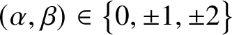 $(\alpha ,\beta ) \in \bigl \{ 0, \pm 1, \pm 2\bigr \}$
. In addition,
$(\alpha ,\beta ) \in \bigl \{ 0, \pm 1, \pm 2\bigr \}$
. In addition,
 $(\alpha ,\beta ) = \pm 2$
if and only if
$(\alpha ,\beta ) = \pm 2$
if and only if
 $\alpha =\pm \beta $
.
$\alpha =\pm \beta $
.
Lemma B.2.
-
1.
$(\lambda ,\beta _{r}) = -1$
for all
$1 \le r \le l$
. -
2.
$(\beta _{r},\beta _{t}) \in \bigl \{0,1\bigr \}$
for all
$1 \le r$
,
$t \le l$
with
$r \ne t$
.


Proof. (1) We see that
 $$ \begin{align*} (\lambda,\beta_{r}) & = \left(s_{j_{l}}s_{j_{l-1}} \cdots s_{j_{2}}s_{j_{1}}\varpi_{k}, s_{j_{l}}s_{j_{l-1}} \cdots s_{j_{r+1}}\left(\alpha_{j_{r}}\right) \right) \\ & = \Big(\underbrace{ s_{j_{r}}s_{j_{r-1}} \cdots s_{j_{2}}s_{j_{1}} }_{=:v} \varpi_{k},\,\alpha_{j_{r}}\Big) = \left(\varpi_{k},v^{-1}\alpha_{j_{r}}\right). \end{align*} $$
Since
 $v=s_{j_{r}}s_{j_{r-1}} \cdots s_{j_{2}}s_{j_{1}} \in W^{J}$
with
$v=s_{j_{r}}s_{j_{r-1}} \cdots s_{j_{2}}s_{j_{1}} \in W^{J}$
with
 $s_{j_{r}}v < v$
, it follows that
$s_{j_{r}}v < v$
, it follows that
 $v^{-1}\alpha _{j_{r}} \in -\left (\Delta ^{+} \setminus \Delta _{J}^{+}\right )$
. Therefore, we have
$v^{-1}\alpha _{j_{r}} \in -\left (\Delta ^{+} \setminus \Delta _{J}^{+}\right )$
. Therefore, we have
 $\left (\varpi _{k},v^{-1}\alpha _{j_{r}}\right ) < 0$
; since
$\left (\varpi _{k},v^{-1}\alpha _{j_{r}}\right ) < 0$
; since
 $\varpi _{k}$
is minuscule, we obtain
$\varpi _{k}$
is minuscule, we obtain
 $\left (\varpi _{k},v^{-1}\alpha _{j_{r}}\right ) = -1$
, as desired.
$\left (\varpi _{k},v^{-1}\alpha _{j_{r}}\right ) = -1$
, as desired.
(2) By Lemma B.1, we have
 $(\beta _{r},\beta _{t}) \in \bigl \{0,\pm 1\bigr \}$
. Suppose, for a contradiction, that
$(\beta _{r},\beta _{t}) \in \bigl \{0,\pm 1\bigr \}$
. Suppose, for a contradiction, that
 $(\beta _{r},\beta _{t}) = -1$
. Then
$(\beta _{r},\beta _{t}) = -1$
. Then
 $s_{\beta _{r}}(\beta _{t}) = \beta _{r}+\beta _{t} \in \Delta $
. By (1), we have
$s_{\beta _{r}}(\beta _{t}) = \beta _{r}+\beta _{t} \in \Delta $
. By (1), we have
 $(\lambda ,\beta _{r}+\beta _{t}) = -2$
, which contradicts the assumption that
$(\lambda ,\beta _{r}+\beta _{t}) = -2$
, which contradicts the assumption that
 $\varpi _{k}$
is minuscule. This proves the lemma.
$\varpi _{k}$
is minuscule. This proves the lemma.
□
Equation (3.57) follows from Lemma B.2(1). Equation (3.58) follows from equation (3.57) using the Dynkin diagram automorphism
 $\omega :I \rightarrow I$
induced by
$\omega :I \rightarrow I$
induced by
 $w_{\circ }$
(see Appendix B.2).
$w_{\circ }$
(see Appendix B.2).
In Appendices B.1 and B.2, we provide a complete proof of Proposition 3.9, since we do not know of a suitable reference for these assertions.
B.1. Proof of equation (3.59)
For
 $\alpha = \sum _{i \in I}c_{i}\alpha _{i} \in Q$
, we set
$\alpha = \sum _{i \in I}c_{i}\alpha _{i} \in Q$
, we set
 $\mathrm {ht}(\alpha ):=\sum _{i \in I} c_{i} \in \mathbb {Z}$
.
$\mathrm {ht}(\alpha ):=\sum _{i \in I} c_{i} \in \mathbb {Z}$
.
Lemma B.3. Set
 $1 \le r < t \le l$
. If
$1 \le r < t \le l$
. If
 $(\beta _{r},\beta _{t})=1$
, then
$(\beta _{r},\beta _{t})=1$
, then
 $\mathrm {ht}(\beta _{r})> \mathrm {ht}(\beta _{t})$
.
$\mathrm {ht}(\beta _{r})> \mathrm {ht}(\beta _{t})$
.
Proof. We prove the assertion by induction on
 $l=\ell (x)$
. If
$l=\ell (x)$
. If
 $l=0$
or
$l=0$
or
 $l=1$
, then the assertion is obvious. Assume that
$l=1$
, then the assertion is obvious. Assume that
 $l> 1$
. If
$l> 1$
. If
 $t = l$
, then
$t = l$
, then
 $\beta _{t} = \beta _{l} = \alpha _{j_{l}}$
, and
$\beta _{t} = \beta _{l} = \alpha _{j_{l}}$
, and
 $$ \begin{align*} s_{j_{l-1}} \cdots s_{j_{r+1}}\left(\alpha_{j_{r}}\right) = s_{j_{l}} \beta_{r} = s_{\beta_{t}} \beta_{r} = \beta_{r}-\beta_{t}. \end{align*} $$
Hence
 $\beta _{r} = \beta _{t} + s_{j_{l-1}} \cdots s_{j_{r+1}}\left (\alpha _{j_{r}}\right )$
; note that
$\beta _{r} = \beta _{t} + s_{j_{l-1}} \cdots s_{j_{r+1}}\left (\alpha _{j_{r}}\right )$
; note that
 $s_{j_{l-1}} \cdots s_{j_{r+1}}\left (\alpha _{j_{r}}\right ) \in \Delta ^{+}$
, since
$s_{j_{l-1}} \cdots s_{j_{r+1}}\left (\alpha _{j_{r}}\right ) \in \Delta ^{+}$
, since
 $s_{j_{l-1}} \cdots s_{j_{r+1}}s_{j_{r}}$
is reduced. Therefore, we obtain
$s_{j_{l-1}} \cdots s_{j_{r+1}}s_{j_{r}}$
is reduced. Therefore, we obtain
 $\mathrm {ht}(\beta _{r})> \mathrm {ht}(\beta _{t})$
.
$\mathrm {ht}(\beta _{r})> \mathrm {ht}(\beta _{t})$
.
Assume that
 $t \le l-1$
. Note that
$t \le l-1$
. Note that
 $x':=s_{j_{l}}x \in W^{J}$
with
$x':=s_{j_{l}}x \in W^{J}$
with
 $\ell (x') = \ell (x)-1$
, and that
$\ell (x') = \ell (x)-1$
, and that
 $x'=s_{j_{p-1}} \cdots s_{j_{2}}s_{j_{1}}$
is a reduced expression for
$x'=s_{j_{p-1}} \cdots s_{j_{2}}s_{j_{1}}$
is a reduced expression for
 $x'$
. We set
$x'$
. We set
 $$ \begin{align*} \beta_{u}':=s_{j_{l-1}} \cdots s_{j_{u+1}}\left(\alpha_{j_{u}}\right) = s_{j_{l}}\beta_{u} \quad \text{for}\ 1 \le u \le l-1. \end{align*} $$
Since
 $1 \le r < t \le l-1$
satisfy the condition that
$1 \le r < t \le l-1$
satisfy the condition that
 $\left (\beta _{r}',\beta _{t}'\right ) = (\beta _{r},\beta _{t})=1$
, it follows by our induction hypothesis that
$\left (\beta _{r}',\beta _{t}'\right ) = (\beta _{r},\beta _{t})=1$
, it follows by our induction hypothesis that
 $\mathrm {ht}\left (\beta _{r}'\right )> \mathrm {ht}\left (\beta _{t}'\right )$
. Here we remark that
$\mathrm {ht}\left (\beta _{r}'\right )> \mathrm {ht}\left (\beta _{t}'\right )$
. Here we remark that
 $$ \begin{align*} \beta_{r} = \beta_{r}' - \underbrace{\left(\beta_{r}',\alpha_{j_{l}}\right)}_{=:a} \alpha_{j_{l}}, \qquad \beta_{t} = \beta_{t}' - \underbrace{\left(\beta_{t}',\alpha_{j_{l}}\right)}_{=:b} \alpha_{j_{l}}, \end{align*} $$
where
 $a,b \in \{0,-1\}$
by Lemma B.2(2). If
$a,b \in \{0,-1\}$
by Lemma B.2(2). If
 $a=-1$
or if
$a=-1$
or if
 $a=b=0$
, then it is obvious that
$a=b=0$
, then it is obvious that
 $\mathrm {ht}(\beta _{r})> \mathrm {ht}(\beta _{t})$
, since
$\mathrm {ht}(\beta _{r})> \mathrm {ht}(\beta _{t})$
, since
 $\mathrm {ht}\left (\beta ^{\prime }_{r}\right )> \mathrm {ht}\left (\beta ^{\prime }_{t}\right )$
by our induction hypothesis. Assume that
$\mathrm {ht}\left (\beta ^{\prime }_{r}\right )> \mathrm {ht}\left (\beta ^{\prime }_{t}\right )$
by our induction hypothesis. Assume that
 $a=0$
and
$a=0$
and
 $b=-1$
. Suppose, for a contradiction, that
$b=-1$
. Suppose, for a contradiction, that
 $\mathrm {ht}(\beta _{r}) \le \mathrm {ht}(\beta _{t})$
. Since
$\mathrm {ht}(\beta _{r}) \le \mathrm {ht}(\beta _{t})$
. Since
 $\mathrm {ht}(\beta _{t}) = \mathrm {ht}\left (\beta ^{\prime }_{t}\right ) + 1$
and
$\mathrm {ht}(\beta _{t}) = \mathrm {ht}\left (\beta ^{\prime }_{t}\right ) + 1$
and
 $\mathrm {ht}(\beta _{r}) = \mathrm {ht}\left (\beta ^{\prime }_{r}\right )$
, and since
$\mathrm {ht}(\beta _{r}) = \mathrm {ht}\left (\beta ^{\prime }_{r}\right )$
, and since
 $\mathrm {ht}\left (\beta ^{\prime }_{r}\right )> \mathrm {ht}\left (\beta ^{\prime }_{t}\right )$
by our induction hypothesis, we have
$\mathrm {ht}\left (\beta ^{\prime }_{r}\right )> \mathrm {ht}\left (\beta ^{\prime }_{t}\right )$
by our induction hypothesis, we have
 $\mathrm {ht}(\beta _{r}) = \mathrm {ht}(\beta _{t})$
. Since
$\mathrm {ht}(\beta _{r}) = \mathrm {ht}(\beta _{t})$
. Since
 $(\beta _{r},\beta _{t})=1$
by the assumption, we see that
$(\beta _{r},\beta _{t})=1$
by the assumption, we see that
 $\beta _{r}-\beta _{t} \in \Delta $
. However,
$\beta _{r}-\beta _{t} \in \Delta $
. However,
 $\mathrm {ht}(\beta _{r}-\beta _{t}) =\mathrm {ht}(\beta _{r})-\mathrm {ht}(\beta _{t})=0$
, which is a contradiction. Hence we conclude that
$\mathrm {ht}(\beta _{r}-\beta _{t}) =\mathrm {ht}(\beta _{r})-\mathrm {ht}(\beta _{t})=0$
, which is a contradiction. Hence we conclude that
 $\mathrm {ht}(\beta _{r})> \mathrm {ht}(\beta _{t})$
, as desired. This proves the lemma.□
$\mathrm {ht}(\beta _{r})> \mathrm {ht}(\beta _{t})$
, as desired. This proves the lemma.□
Lemma B.4. Set
 $1 \le r \le l$
, and set
$1 \le r \le l$
, and set
 $h:=\mathrm {ht}(\beta _{r})$
. Then
$h:=\mathrm {ht}(\beta _{r})$
. Then
 $$ \begin{align} & \# \{ r < t \le l \mid (\beta_{t},\beta_{r})=1\}=h-1, \end{align} $$
 $$ \begin{align} & \# \left\{ \alpha \in \Delta^{+} \mid \mathrm{ht}(\alpha) < \mathrm{ht}(\beta_{r}), (\alpha,\beta_{r})=1 \right\} = 2(h-1). \end{align} $$
Proof. We prove the assertion by induction on
 $l=\ell (x)$
. If
$l=\ell (x)$
. If
 $l=0$
or
$l=0$
or
 $l=1$
, then the assertion is obvious. Assume that
$l=1$
, then the assertion is obvious. Assume that
 $l> 1$
. If
$l> 1$
. If
 $r = l$
, then the assertion is obvious. Assume now that
$r = l$
, then the assertion is obvious. Assume now that
 $1 \le r \le l-1$
. Note that
$1 \le r \le l-1$
. Note that
 $x':=s_{j_{l}}x \in W^{J}$
with
$x':=s_{j_{l}}x \in W^{J}$
with
 $\ell (x') = \ell (x)-1$
, and that
$\ell (x') = \ell (x)-1$
, and that
 $x'=s_{j_{l-1}} \cdots s_{j_{2}}s_{j_{1}}$
is a reduced expression for
$x'=s_{j_{l-1}} \cdots s_{j_{2}}s_{j_{1}}$
is a reduced expression for
 $x'$
. We set
$x'$
. We set
 $$ \begin{align*} \beta_{u}':=s_{j_{l-1}} \cdots s_{j_{u+1}}\left(\alpha_{j_{u}}\right) = s_{j_{l}}\beta_{u} \quad \text{for}\ 1 \le u \le l-1. \end{align*} $$
Since
 $\beta _{l}=\alpha _{j_{l}}$
, we see by Lemma B.2(2) that
$\beta _{l}=\alpha _{j_{l}}$
, we see by Lemma B.2(2) that
 $\left (\beta _{r}', \alpha _{j_{l}}\right ) = - \left (\beta _{r},\alpha _{j_{l}}\right ) = - (\beta _{r},\beta _{l}) \in \{0,-1\}$
.
$\left (\beta _{r}', \alpha _{j_{l}}\right ) = - \left (\beta _{r},\alpha _{j_{l}}\right ) = - (\beta _{r},\beta _{l}) \in \{0,-1\}$
.
Case 1. Assume first that
 $\left (\beta _{r}', \alpha _{j_{l}}\right ) = 0$
, or equivalently,
$\left (\beta _{r}', \alpha _{j_{l}}\right ) = 0$
, or equivalently,
 $\left (\beta _{r}, \alpha _{j_{l}}\right ) = 0$
; in this case,
$\left (\beta _{r}, \alpha _{j_{l}}\right ) = 0$
; in this case,
 $\beta _{r}=\beta _{r}'$
, and hence
$\beta _{r}=\beta _{r}'$
, and hence
 $\mathrm {ht}\left (\beta _{r}'\right )=\mathrm {ht}(\beta _{r})=h$
. In addition, since
$\mathrm {ht}\left (\beta _{r}'\right )=\mathrm {ht}(\beta _{r})=h$
. In addition, since
 $\beta _{l}=\alpha _{j_{l}}$
, it follows that
$\beta _{l}=\alpha _{j_{l}}$
, it follows that
 $$ \begin{align*} \{ r < t \le l \mid (\beta_{t},\beta_{r})=1\} & = \{ r < t \le l-1 \mid (\beta_{t},\beta_{r})=1\} \\ & = \left\{ r < t \le l-1 \mid \left(s_{j_{l}}\beta_{t},s_{j_{l}}\beta_{r}\right)=1\right\} \\ & = \left\{ r < t \le l-1 \mid \left(\beta_{t}',\beta_{r}'\right)=1\right\}\!. \end{align*} $$
By our induction hypothesis, we have
 $\# \left \{ r < t \le l-1 \mid \left (\beta _{t}',\beta _{r}'\right )=1\right \} = h-1$
, and hence
$\# \left \{ r < t \le l-1 \mid \left (\beta _{t}',\beta _{r}'\right )=1\right \} = h-1$
, and hence
 $\# \{ r < t \le l \mid (\beta _{t},\beta _{r})=1\} =h-1$
, as desired. Also, since
$\# \{ r < t \le l \mid (\beta _{t},\beta _{r})=1\} =h-1$
, as desired. Also, since
 $\beta _{r}=\beta _{r}'$
in this case, it is obvious that
$\beta _{r}=\beta _{r}'$
in this case, it is obvious that
 $$ \begin{align*} & \left\{ \alpha \in \Delta^{+} \mid \mathrm{ht}(\alpha) < \mathrm{ht}(\beta_{r}), (\alpha,\beta_{r})=1\right\} = \left\{ \alpha \in \Delta^{+} \mid \mathrm{ht}(\alpha) < \mathrm{ht}\left(\beta^{\prime}_{r}\right), \left(\alpha,\beta^{\prime}_{r}\right)=1\right\}\!. \end{align*} $$
Since
 $\# \left \{ \alpha \in \Delta ^{+} \mid \mathrm {ht}(\alpha ) < \mathrm {ht}\left (\beta ^{\prime }_{r}\right ), \left (\alpha ,\beta ^{\prime }_{r}\right )=1\right \}= 2(h-1)$
by our induction hypothesis, we obtain equation (B.3), as desired.
$\# \left \{ \alpha \in \Delta ^{+} \mid \mathrm {ht}(\alpha ) < \mathrm {ht}\left (\beta ^{\prime }_{r}\right ), \left (\alpha ,\beta ^{\prime }_{r}\right )=1\right \}= 2(h-1)$
by our induction hypothesis, we obtain equation (B.3), as desired.
Case 2. Assume next that
 $\left (\beta ^{\prime }_{r}, \alpha _{j_{l}}\right ) = -1$
, or equivalently,
$\left (\beta ^{\prime }_{r}, \alpha _{j_{l}}\right ) = -1$
, or equivalently,
 $\left (\beta _{r}, \alpha _{j_{l}}\right ) = 1$
; in this case,
$\left (\beta _{r}, \alpha _{j_{l}}\right ) = 1$
; in this case,
 $\beta _{r}=\beta ^{\prime }_{r}+\alpha _{j_{l}}$
, and hence
$\beta _{r}=\beta ^{\prime }_{r}+\alpha _{j_{l}}$
, and hence
 $\mathrm {ht}\left (\beta ^{\prime }_{r}\right )=\mathrm {ht}(\beta _{r})-1=h-1$
. In addition, since
$\mathrm {ht}\left (\beta ^{\prime }_{r}\right )=\mathrm {ht}(\beta _{r})-1=h-1$
. In addition, since
 $\beta _{l}=\alpha _{j_{l}}$
, it follows that
$\beta _{l}=\alpha _{j_{l}}$
, it follows that
 $$ \begin{align*} \{ r < t \le l \mid (\beta_{t},\beta_{r})=1\} & = \{ r < t \le l-1 \mid (\beta_{t},\beta_{r})=1\} \cup \{l\} \\ & = \left\{ r < t \le l-1 \mid \left(s_{j_{l}}\beta_{t},s_{j_{l}}\beta_{r}\right)=1\right\} \cup \{l\} \\ & = \left\{ r < t \le l-1 \mid \left(\beta_{t}',\beta_{r}'\right)=1\right\} \cup \{l\}. \end{align*} $$
By our induction hypothesis, we have
 $\# \left \{ r < t \le l-1 \mid \left (\beta _{t}',\beta _{r}'\right )=1\right \} = h-2$
, and hence
$\# \left \{ r < t \le l-1 \mid \left (\beta _{t}',\beta _{r}'\right )=1\right \} = h-2$
, and hence
 $\# \{ r < t \le l \mid (\beta _{t},\beta _{r})=1\} = h-1$
, as desired.
$\# \{ r < t \le l \mid (\beta _{t},\beta _{r})=1\} = h-1$
, as desired.
Let us prove equation (B.3) in this case. For simplicity of notation, we set
 $$ \begin{align} & R=R_{r}:= \left\{ \alpha \in \Delta^{+} \mid \mathrm{ht}(\alpha) < \mathrm{ht}(\beta_{r}), (\alpha,\beta_{r})=1\right\}\kern-2pt, \nonumber\\ & S=S_{r}:= \left\{ \alpha \in \Delta^{+} \mid \mathrm{ht}(\alpha) < \mathrm{ht}\left(\beta^{\prime}_{r}\right), \left(\alpha,\beta^{\prime}_{r}\right)=1\right\}\kern-2pt. \end{align} $$
Since
 $\left (\beta _{r}, \alpha _{j_{l}}\right ) = 1$
and
$\left (\beta _{r}, \alpha _{j_{l}}\right ) = 1$
and
 $\beta _{r}-\alpha _{j_{l}} = s_{j_{l}}\beta _{r} = \beta ^{\prime }_{r} \in \Delta ^{+}$
, we deduce that
$\beta _{r}-\alpha _{j_{l}} = s_{j_{l}}\beta _{r} = \beta ^{\prime }_{r} \in \Delta ^{+}$
, we deduce that
 $\alpha _{j_{l}},\,\beta _{r}-\alpha _{j_{l}} \in R$
. We claim that
$\alpha _{j_{l}},\,\beta _{r}-\alpha _{j_{l}} \in R$
. We claim that
 $$ \begin{align} s_{j_{l}}\alpha \in S \quad \text{for all}\ \alpha \in R \setminus \left\{ \alpha_{j_{l}}, \beta_{r}-\alpha_{j_{l}} \right\}\kern-2pt. \end{align} $$
It is easily verified that
 $s_{j_{l}}\alpha \in \Delta ^{+}$
and
$s_{j_{l}}\alpha \in \Delta ^{+}$
and
 $\left (s_{j_{l}}\alpha ,\beta ^{\prime }_{r}\right ) = 1$
. We show that
$\left (s_{j_{l}}\alpha ,\beta ^{\prime }_{r}\right ) = 1$
. We show that
 $\mathrm {ht}\left (s_{j_{l}} \alpha \right ) < \mathrm {ht}\left (\beta ^{\prime }_{r}\right )$
. By Lemma B.1,
$\mathrm {ht}\left (s_{j_{l}} \alpha \right ) < \mathrm {ht}\left (\beta ^{\prime }_{r}\right )$
. By Lemma B.1,
 $\left (\alpha ,\alpha _{j_{l}}\right ) \in \{0,\pm 1\}$
. If
$\left (\alpha ,\alpha _{j_{l}}\right ) \in \{0,\pm 1\}$
. If
 $\left (\alpha ,\alpha _{j_{l}}\right ) = 1$
, then it is obvious that
$\left (\alpha ,\alpha _{j_{l}}\right ) = 1$
, then it is obvious that
 $\mathrm {ht}\left (s_{j_{l}} \alpha \right ) < \mathrm {ht}\left (\beta ^{\prime }_{r}\right )$
. Assume that
$\mathrm {ht}\left (s_{j_{l}} \alpha \right ) < \mathrm {ht}\left (\beta ^{\prime }_{r}\right )$
. Assume that
 $\left (\alpha ,\alpha _{j_{l}}\right ) = 0$
. Suppose, for a contradiction, that
$\left (\alpha ,\alpha _{j_{l}}\right ) = 0$
. Suppose, for a contradiction, that
 $\mathrm {ht}\left (s_{j_{l}} \alpha \right ) \ge \mathrm {ht}\left (\beta ^{\prime }_{r}\right )$
. Since
$\mathrm {ht}\left (s_{j_{l}} \alpha \right ) \ge \mathrm {ht}\left (\beta ^{\prime }_{r}\right )$
. Since
 $\mathrm {ht}(\alpha ) < \mathrm {ht}(\beta _{r})$
and
$\mathrm {ht}(\alpha ) < \mathrm {ht}(\beta _{r})$
and
 $\mathrm {ht}\left (\beta ^{\prime }_{r}\right ) = \mathrm {ht}(\beta _{r}) -1$
, we have
$\mathrm {ht}\left (\beta ^{\prime }_{r}\right ) = \mathrm {ht}(\beta _{r}) -1$
, we have
 $\mathrm {ht}\left (s_{j_{l}} \alpha \right ) = \mathrm {ht}\left (\beta ^{\prime }_{r}\right )$
. Since
$\mathrm {ht}\left (s_{j_{l}} \alpha \right ) = \mathrm {ht}\left (\beta ^{\prime }_{r}\right )$
. Since
 $\left (s_{j_{l}} \alpha ,\beta ^{\prime }_{r}\right )=1$
, we see that
$\left (s_{j_{l}} \alpha ,\beta ^{\prime }_{r}\right )=1$
, we see that
 $\beta ^{\prime }_{r} - s_{j_{l}} \alpha \in \Delta $
. However,
$\beta ^{\prime }_{r} - s_{j_{l}} \alpha \in \Delta $
. However,
 $\mathrm {ht}\left (\beta ^{\prime }_{r} - s_{j_{l}} \alpha \right ) =0$
, which is a contradiction. Assume that
$\mathrm {ht}\left (\beta ^{\prime }_{r} - s_{j_{l}} \alpha \right ) =0$
, which is a contradiction. Assume that
 $\left (\alpha ,\alpha _{j_{l}}\right ) = -1$
; in this case,
$\left (\alpha ,\alpha _{j_{l}}\right ) = -1$
; in this case,
 $s_{j_{l}}\alpha = \alpha +\alpha _{j_{l}}$
. Suppose, for a contradiction, that
$s_{j_{l}}\alpha = \alpha +\alpha _{j_{l}}$
. Suppose, for a contradiction, that
 $\mathrm {ht}\left (s_{j_{l}}\alpha \right ) \ge \mathrm {ht}\left (\beta ^{\prime }_{r}\right )$
; since
$\mathrm {ht}\left (s_{j_{l}}\alpha \right ) \ge \mathrm {ht}\left (\beta ^{\prime }_{r}\right )$
; since
 $\mathrm {ht}\left (s_{j_{l}}\alpha \right ) = \mathrm {ht}(\alpha )+1$
and
$\mathrm {ht}\left (s_{j_{l}}\alpha \right ) = \mathrm {ht}(\alpha )+1$
and
 $\mathrm {ht}\left (\beta ^{\prime }_{r}\right ) = \mathrm {ht}(\beta _{r})-1$
, and since
$\mathrm {ht}\left (\beta ^{\prime }_{r}\right ) = \mathrm {ht}(\beta _{r})-1$
, and since
 $\mathrm {ht}(\alpha ) < \mathrm {ht}(\beta _{r})$
,
$\mathrm {ht}(\alpha ) < \mathrm {ht}(\beta _{r})$
,
 $\mathrm {ht}\left (s_{j_{l}}\alpha \right )$
is equal to
$\mathrm {ht}\left (s_{j_{l}}\alpha \right )$
is equal to
 $\mathrm {ht}\left (\beta ^{\prime }_{r}\right )$
or
$\mathrm {ht}\left (\beta ^{\prime }_{r}\right )$
or
 $\mathrm {ht}\left (\beta ^{\prime }_{r}\right )+1$
. By the same reasoning as before, we see that
$\mathrm {ht}\left (\beta ^{\prime }_{r}\right )+1$
. By the same reasoning as before, we see that
 $\mathrm {ht}\left (s_{j_{l}}\alpha \right ) \ne \mathrm {ht}\left (\beta ^{\prime }_{r}\right )$
. Therefore,
$\mathrm {ht}\left (s_{j_{l}}\alpha \right ) \ne \mathrm {ht}\left (\beta ^{\prime }_{r}\right )$
. Therefore,
 $\mathrm {ht}\left (s_{j_{l}}\alpha \right ) = \mathrm {ht}\left (\beta ^{\prime }_{r}\right )+1$
, and hence
$\mathrm {ht}\left (s_{j_{l}}\alpha \right ) = \mathrm {ht}\left (\beta ^{\prime }_{r}\right )+1$
, and hence
 $\mathrm {ht}(\alpha )=\mathrm {ht}(\beta _{r})-1$
. Also, we see that
$\mathrm {ht}(\alpha )=\mathrm {ht}(\beta _{r})-1$
. Also, we see that
 $s_{\alpha }\beta _{r} = \beta _{r}-\alpha \in \Delta ^{+}$
. From these, we deduce that
$s_{\alpha }\beta _{r} = \beta _{r}-\alpha \in \Delta ^{+}$
. From these, we deduce that
 $\alpha = \beta _{r}-\alpha _{j}$
for some
$\alpha = \beta _{r}-\alpha _{j}$
for some
 $j \in I$
. It follows that
$j \in I$
. It follows that
 $$ \begin{align*} -1 = \left(\alpha,\alpha_{j_{l}}\right) = \left(\beta_{r},\alpha_{j_{l}}\right)- \left(\alpha_{j},\alpha_{j_{l}}\right) = 1 - \left(\alpha_{j},\alpha_{j_{l}}\right)\kern-2pt, \end{align*} $$
and hence
 $\left (\alpha _{j},\alpha _{j_{l}}\right ) = 2$
. This implies that
$\left (\alpha _{j},\alpha _{j_{l}}\right ) = 2$
. This implies that
 $j = j_{l}$
, and hence
$j = j_{l}$
, and hence
 $\alpha = \beta _{r}-\alpha _{j_{l}}$
, which is a contradiction. Thus, we have shown that
$\alpha = \beta _{r}-\alpha _{j_{l}}$
, which is a contradiction. Thus, we have shown that
 $\mathrm {ht}\left (s_{j_{l}} \alpha \right ) < \mathrm {ht}\left (\beta ^{\prime }_{r}\right )$
in all cases. Therefore, we obtain a map
$\mathrm {ht}\left (s_{j_{l}} \alpha \right ) < \mathrm {ht}\left (\beta ^{\prime }_{r}\right )$
in all cases. Therefore, we obtain a map
 $$ \begin{align*} s_{j_{l}} : R \setminus \left\{ \alpha_{j_{l}}, \beta_{r}-\alpha_{j_{l}} \right\} \rightarrow S, \qquad \alpha \mapsto s_{j_{l}}\alpha. \end{align*} $$
Similarly, we obtain its inverse
 $$ \begin{align*} s_{j_{l}} : S \rightarrow R \setminus \left\{ \alpha_{j_{l}}, \beta_{r}-\alpha_{j_{l}} \right\}, \qquad \alpha \mapsto s_{j_{l}}\alpha. \end{align*} $$
Recall that
 $\mathrm {ht}\left (\beta ^{\prime }_{r}\right )=\mathrm {ht}(\beta _{r})-1=h-1$
. We conclude that
$\mathrm {ht}\left (\beta ^{\prime }_{r}\right )=\mathrm {ht}(\beta _{r})-1=h-1$
. We conclude that
 $$ \begin{align*} \# R & = \# \left(R \setminus \left\{ \alpha_{j_{l}}, \beta_{r}-\alpha_{j_{l}} \right\}\right) + 2 \\ & = \# S + 2 = 2(h-2) + 2 = 2(h-1), \end{align*} $$
as desired. This proves the lemma.□
Remark B.5. Keep the notation and setting as before. Set
 $1 \le r \le l$
. We set
$1 \le r \le l$
. We set
 $$ \begin{align} R_{r}:= \left\{ \alpha \in \Delta^{+} \mid \mathrm{ht}(\alpha) < \mathrm{ht}(\beta_{r}), (\alpha,\beta_{r})=1\right\}\kern-2pt. \end{align} $$
If
 $\alpha \in R_{r}$
, then
$\alpha \in R_{r}$
, then
 $s_{\alpha }\beta _{r} = \beta _{r}-\alpha \in \Delta ^{+}$
; it is easily verified that
$s_{\alpha }\beta _{r} = \beta _{r}-\alpha \in \Delta ^{+}$
; it is easily verified that
 $\beta _{r}-\alpha \in R_{r}$
. Hence
$\beta _{r}-\alpha \in R_{r}$
. Hence
 $\sigma :\alpha \mapsto \beta _{r}-\alpha $
is an involution on
$\sigma :\alpha \mapsto \beta _{r}-\alpha $
is an involution on
 $R_{r}$
; notice that
$R_{r}$
; notice that
 $\sigma $
is fixed-point-free (otherwise,
$\sigma $
is fixed-point-free (otherwise,
 $\beta _{r}=2\alpha $
for some
$\beta _{r}=2\alpha $
for some
 $\alpha \in R_{r}$
). By Lemma B.3,
$\alpha \in R_{r}$
). By Lemma B.3,
 $$ \begin{align*} B_{r}:= \{ \beta_{t} \mid r < t \le l,\,(\beta_{t},\beta_{r})=1\} \end{align*} $$
is a subset of
 $R_{r}$
; recall from Lemma B.4 that
$R_{r}$
; recall from Lemma B.4 that
 $\#B_{r}=h-1$
and
$\#B_{r}=h-1$
and
 $\#R_{r}=2(h-1)$
, where
$\#R_{r}=2(h-1)$
, where
 $h:=\mathrm {ht}(\beta _{r})$
. We claim that
$h:=\mathrm {ht}(\beta _{r})$
. We claim that
 $\sigma (B_{r}) \sqcup B_{r} = R_{r}$
. Suppose, for a contradiction, that
$\sigma (B_{r}) \sqcup B_{r} = R_{r}$
. Suppose, for a contradiction, that
 $\sigma (\beta _{t}) = \beta _{r}-\beta _{t} \in B_{r}$
for some
$\sigma (\beta _{t}) = \beta _{r}-\beta _{t} \in B_{r}$
for some
 $\beta _{t} \in B_{r}$
. Let
$\beta _{t} \in B_{r}$
. Let
 $r < s \le l$
be such that
$r < s \le l$
be such that
 $\sigma (\beta _{t}) = \beta _{s}$
. Then
$\sigma (\beta _{t}) = \beta _{s}$
. Then
 $\beta _{r} = \beta _{s}+\beta _{t}$
, and hence
$\beta _{r} = \beta _{s}+\beta _{t}$
, and hence
 $(\lambda ,\beta _{r}) = (\lambda , \beta _{s})+(\lambda ,\beta _{t}) = -2$
by Lemma B.2(1). However, this contradicts the assumption that
$(\lambda ,\beta _{r}) = (\lambda , \beta _{s})+(\lambda ,\beta _{t}) = -2$
by Lemma B.2(1). However, this contradicts the assumption that
 $\lambda $
is minuscule. It follows that
$\lambda $
is minuscule. It follows that
 $\sigma (B_{r}) \cap B_{r} = \emptyset $
, and hence
$\sigma (B_{r}) \cap B_{r} = \emptyset $
, and hence
 $\# ( \sigma (B_{r}) \cup B_{r} ) = 2(h-1) = \# R_{r}$
. Thus, we conclude that
$\# ( \sigma (B_{r}) \cup B_{r} ) = 2(h-1) = \# R_{r}$
. Thus, we conclude that
 $\sigma (B_{r}) \sqcup B_{r} = R_{r}$
.
$\sigma (B_{r}) \sqcup B_{r} = R_{r}$
.
We will prove equation (3.59). For
 $v \in \left \{w,\,s_{\beta _{r}}w\right \}$
, we set
$v \in \left \{w,\,s_{\beta _{r}}w\right \}$
, we set
 $$ \begin{align*} X(v) & := \left\{ \gamma \in \mathrm{Inv}(v) \mid s_{\beta_{r}}\gamma \in \Delta^{+} \right\}\kern-2pt, \\ Y(v) & := \left\{ \gamma \in \mathrm{Inv}(v) \mid s_{\beta_{r}}\gamma \in \Delta^{-} \right\}\kern-2pt. \end{align*} $$
Note that
 $\mathrm {Inv} (v) = X(v) \sqcup Y(v)$
for
$\mathrm {Inv} (v) = X(v) \sqcup Y(v)$
for
 $v \in \left \{w,s_{\beta _{r}}w\right \}$
. We see that the map
$v \in \left \{w,s_{\beta _{r}}w\right \}$
. We see that the map
 $X(w) \rightarrow X\left (s_{\beta _{r}}w\right )$
,
$X(w) \rightarrow X\left (s_{\beta _{r}}w\right )$
,
 $\gamma \mapsto s_{\beta _{r}}\gamma $
, is bijective. Therefore,
$\gamma \mapsto s_{\beta _{r}}\gamma $
, is bijective. Therefore,
 $$ \begin{align*} \ell(w)-\ell\left(s_{\beta_{r}}w\right) = \# Y(w) - \# Y\left(s_{\beta_{r}}w\right). \end{align*} $$
Also, by Lemma B.1 and the assumption that
 $s_{\beta _{r}}w < w$
, it follows that
$s_{\beta _{r}}w < w$
, it follows that
 $$ \begin{align*} Y(w) = \{ \beta_{r} \} \sqcup (\mathrm{Inv} (w) \cap R_{r}), \qquad Y\left(s_{\beta_{r}} w\right) = \mathrm{Inv}\left(s_{\beta_{r}}w\right) \cap R_{r} \end{align*} $$
(for the definition of
 $R_{r}$
, see Remark B.5). Recall from Remark B.5 that for
$R_{r}$
, see Remark B.5). Recall from Remark B.5 that for
 $\beta _{t} \in B_{r}$
,
$\beta _{t} \in B_{r}$
,
 $\sigma (\beta _{t}) = \beta _{r}-\beta _{t} \in R_{r} \setminus B_{r}$
, and that
$\sigma (\beta _{t}) = \beta _{r}-\beta _{t} \in R_{r} \setminus B_{r}$
, and that
 $R_{r}=B_{r} \sqcup \sigma (B_{r})$
. Since
$R_{r}=B_{r} \sqcup \sigma (B_{r})$
. Since
 $\beta _{r} \in \mathrm {Inv}(w)$
, for each
$\beta _{r} \in \mathrm {Inv}(w)$
, for each
 $\beta _{t} \in B_{r}$
, one of the following holds:
$\beta _{t} \in B_{r}$
, one of the following holds:
-
(i)
$\beta _{t},\sigma (\beta _{t}) \in \mathrm {Inv}(w)$
. -
(ii)
$\beta _{t} \in \mathrm {Inv}(w)$
and
$\sigma (\beta _{t}) \not \in \mathrm {Inv}(w)$
. -
(iii)
$\beta _{t} \not \in \mathrm {Inv}(w)$
and
$\sigma (\beta _{t}) \in \mathrm {Inv}(w)$
.
We see that these are equivalent, respectively, to the following:
-
(i)’
$\beta _{t},\sigma (\beta _{t}) \not \in \mathrm {Inv}\left (s_{\beta _{r}}w\right )$
. -
(ii)’
$\beta _{t} \in \mathrm {Inv}\left (s_{\beta _{r}}w\right )$
and
$\sigma (\beta _{t}) \not \in \mathrm {Inv}\left (s_{\beta _{r}}w\right )$
. -
(iii)’
$\beta _{t} \not \in \mathrm {Inv}\left (s_{\beta _{r}}w\right )$
and
$\sigma (\beta _{t}) \in \mathrm {Inv}\left (s_{\beta _{r}}w\right )$
.

Therefore, if we set
 $$ \begin{align*} & a:=\# \{ \beta_{t} \in B_{r} \mid \beta_{t},\sigma(\beta_{t}) \in \mathrm{Inv}(w) \}, \\ & b:=\# \{ \beta_{t} \in B_{r} \mid \beta_{t} \in \mathrm{Inv}(w), \sigma(\beta_{t}) \not\in \mathrm{Inv}(w) \}, \\ & c:=\# \{ \beta_{t} \in B_{r} \mid \beta_{t} \notin \mathrm{Inv}(w), \sigma(\beta_{t}) \in \mathrm{Inv}(w) \}, \end{align*} $$
we have
 $$ \begin{align*} \# Y(w) & = 1 + \#(\mathrm{Inv} (w) \cap R_{r}) = 1 + 2a + b + c, \\ \# Y\left(s_{\beta_{r}}w\right) & = \#\left(\mathrm{Inv} \left(s_{\beta_{r}}w\right) \cap R_{r}\right) = b + c, \end{align*} $$
and hence
 $$ \begin{align} \ell(w)-\ell\left(s_{\beta_{r}}w\right) = \# Y(w) - \# Y\left(s_{\beta_{r}}w\right) = 1+2a. \end{align} $$
Now we see that
 $$ \begin{align*} & \ell_{\lambda,r}^{-}(w)-\ell_{\lambda,r}^{-}\left(s_{\beta_{r}}w\right) \\ & \quad = \# ( \mathrm{Inv}(w) \cap \{\beta_{r},\beta_{r+1},\dots,\beta_{l}\} ) - \# \left( \mathrm{Inv}\left(s_{\beta_{r}}w\right) \cap \{\beta_{r},\beta_{r+1},\dots,\beta_{l}\} \right) \\ & \quad = \# (\{ \beta_{r} \} \sqcup (\mathrm{Inv}(w) \cap \{\beta_{r+1},\dots,\beta_{l}\} )) - \# \left( \mathrm{Inv}\left(s_{\beta_{r}}w\right) \cap \{\beta_{r+1},\dots,\beta_{l}\} \right)=:(\ast), \end{align*} $$
where the last equality follows from the assumption that
 $s_{\beta _{r}}w < w$
. Also, we deduce that for
$s_{\beta _{r}}w < w$
. Also, we deduce that for
 $r < s \le l$
with
$r < s \le l$
with
 $(\beta _{s}, \beta _{r})=0$
,
$(\beta _{s}, \beta _{r})=0$
,
 $\beta _{s} \in \mathrm {Inv}(w)$
if and only if
$\beta _{s} \in \mathrm {Inv}(w)$
if and only if
 $\beta _{s} \in \mathrm {Inv}\left (s_{\beta _{r}}w\right )$
. Therefore,
$\beta _{s} \in \mathrm {Inv}\left (s_{\beta _{r}}w\right )$
. Therefore,
 $$ \begin{align*} (\ast) & = 1 + \# (\mathrm{Inv}(w) \cap B_{r}) - \# \left(\mathrm{Inv}\left(s_{\beta_{r}}w\right) \cap B_{r}\right) \\ & = 1 + (a+b) - b = 1+a. \end{align*} $$
Thus we conclude that
 $$ \begin{align*} 2 \left( \ell_{\lambda,r}^{-}(w)-\ell_{\lambda,r}^{-}\left(s_{\beta_{r}}w\right) \right) - 1 =2 ( 1+a ) - 1 = 2a+1 \stackrel{(B.7)}{=} \ell(w)-\ell\left(s_{\beta_{r}}w\right), \end{align*} $$
as desired. This proves equation (3.59).
B.2. Proofs of equations (3.58) and (3.60)
Let
 $\omega :I \rightarrow I$
be the Dynkin diagram automorphism induced by the longest element
$\omega :I \rightarrow I$
be the Dynkin diagram automorphism induced by the longest element
 $w_{\circ }$
– that is,
$w_{\circ }$
– that is,
 $w_{\circ } \alpha _{i}= -\alpha _{\omega (i)}$
for
$w_{\circ } \alpha _{i}= -\alpha _{\omega (i)}$
for
 $i \in I$
; note that
$i \in I$
; note that
 $\left \lfloor w_{\circ } \right \rfloor \varpi _{k} = w_{\circ } \varpi _{k} = - \varpi _{\omega (k)}$
. We see that
$\left \lfloor w_{\circ } \right \rfloor \varpi _{k} = w_{\circ } \varpi _{k} = - \varpi _{\omega (k)}$
. We see that
 $\varpi _{\omega (k)}$
is also minuscule. In addition,
$\varpi _{\omega (k)}$
is also minuscule. In addition,
 $y^{-1}=s_{i_{m}} \cdots s_{i_{1}} \in W^{\omega (J)} = W^{I \setminus \{\omega (k)\}}$
. We set
$y^{-1}=s_{i_{m}} \cdots s_{i_{1}} \in W^{\omega (J)} = W^{I \setminus \{\omega (k)\}}$
. We set
 $\nu :=y^{-1}\varpi _{\omega (k)}$
; for
$\nu :=y^{-1}\varpi _{\omega (k)}$
; for
 $\gamma \in \Delta ^{+}$
,
$\gamma \in \Delta ^{+}$
,
 $$ \begin{align*} (\gamma,\lambda)=1 \iff \left(\gamma,y^{-1}\left\lfloor w_{\circ} \right\rfloor\varpi_{k}\right)=1 \iff \left(\gamma,y^{-1}\left(-\varpi_{\omega(k)}\right)\right)=1 \iff (\gamma,\nu) = -1. \end{align*} $$
Hence it follows that
 $\mathrm {Inv}(w)_{\lambda }^{+} = \mathrm {Inv}(w)_{\nu }^{-}$
for
$\mathrm {Inv}(w)_{\lambda }^{+} = \mathrm {Inv}(w)_{\nu }^{-}$
for
 $w \in W$
. Also, it is easily verified that
$w \in W$
. Also, it is easily verified that
 $\ell _{\lambda ,s}^{+}(w) = \ell _{\nu ,s}^{-}(w)$
for all
$\ell _{\lambda ,s}^{+}(w) = \ell _{\nu ,s}^{-}(w)$
for all
 $w \in W$
. Thus equations (3.58) and (3.60) follow from equations (3.57) and (3.59) (applied to
$w \in W$
. Thus equations (3.58) and (3.60) follow from equations (3.57) and (3.59) (applied to
 $\nu $
), respectively.
$\nu $
), respectively.
This completes the proof of Proposition 3.9.
Acknowledgements
The authors would like to thank Cristian Lenart, Leonardo Mihalcea and Mark Shimozono for helpful discussions. We also thank an anonymous referee for useful suggestions which improved our exposition. The first author was supported in part by Grant-in-Aid for JSPS Fellows 20J12058. The second author was supported in part by JSPS Grant-in-Aid for Scientific Research (B) 16H03920. The third author was supported in part by a Collaboration Grant for Mathematicians from the Simons Foundation (Award ID: 638577). The fourth author was supported in part by JSPS Grant-in-Aid for Scientific Research (C) 19K03415.
Conflict of Interest
None.


 Open access