Book contents
- Statistical Inference as Severe Testing
- Reviews
- Statistical Inference as Severe Testing
- Copyright page
- Dedication
- Itinerary
- Preface
- Acknowledgments
- Excursion 1 How to Tell What’s True about Statistical Inference
- Excursion 2 Taboos of Induction and Falsification
- Excursion 3 Statistical Tests and Scientific Inference
- Excursion 4 Objectivity and Auditing
- Excursion 5 Power and Severity
- Book part
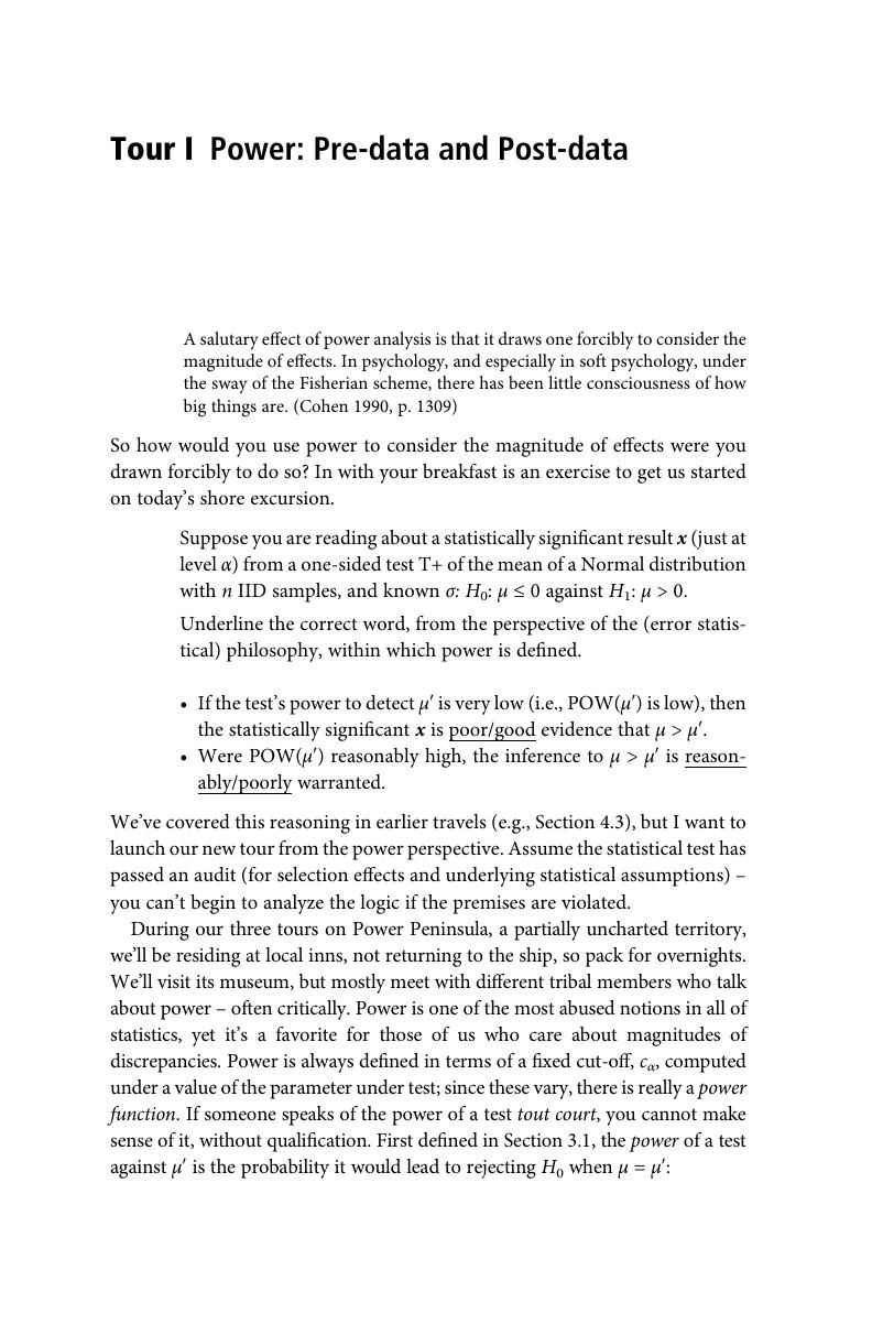
- Tour I Power: Pre-data and Post-data
- Tour II How Not to Corrupt Power
- Tour III Deconstructing the N-P versus Fisher Debates
- Excursion 6 (Probabilist) Foundations Lost, (Probative) Foundations Found
- Souvenirs
- References
- Index
Tour I - Power: Pre-data and Post-data
from Excursion 5 - Power and Severity
Published online by Cambridge University Press: 14 September 2018

Book contents
- Statistical Inference as Severe Testing
- Reviews
- Statistical Inference as Severe Testing
- Copyright page
- Dedication
- Itinerary
- Preface
- Acknowledgments
- Excursion 1 How to Tell What’s True about Statistical Inference
- Excursion 2 Taboos of Induction and Falsification
- Excursion 3 Statistical Tests and Scientific Inference
- Excursion 4 Objectivity and Auditing
- Excursion 5 Power and Severity
- Book part
- Tour I Power: Pre-data and Post-data
- Tour II How Not to Corrupt Power
- Tour III Deconstructing the N-P versus Fisher Debates
- Excursion 6 (Probabilist) Foundations Lost, (Probative) Foundations Found
- Souvenirs
- References
- Index
Summary
A summary is not available for this content so a preview has been provided. Please use the Get access link above for information on how to access this content.
Information
- Type
- Chapter
- Information
- Statistical Inference as Severe TestingHow to Get Beyond the Statistics Wars, pp. 323 - 352Publisher: Cambridge University PressPrint publication year: 2018
Accessibility standard: Unknown
Why this information is here
This section outlines the accessibility features of this content - including support for screen readers, full keyboard navigation and high-contrast display options. This may not be relevant for you.Accessibility Information
Accessibility compliance for the HTML of this chapter is currently unknown
and may be updated in the future.