1 Introduction
Spatial analysis has long been a cornerstone of archaeological research, providing essential insights into how previous populations interacted with and shaped their environments. By examining the spatial relationships between archaeological sites and their surrounding landscapes, researchers can reconstruct patterns of human settlement, economic organization, and environmental adaptation. Traditionally, such analyses have either focused exclusively on the archaeological site itself, through direct excavations and localized surface surveys, or have adopted a broad regional perspective that emphasizes large-scale patterns. However, both approaches have inherent limitations: Site-specific studies tend to overlook the influence of the surrounding landscape, while regional analyses frequently ignore the nuanced, micro-scale interactions that occur in the immediate vicinity of a settlement.
Recent advances in Geographic Information Systems (GIS) have enabled archaeologists to bridge this gap by integrating spatial and geographic data across multiple scales (Bevan and Connolly, Reference Bevan and Connolly2013). Despite these technological improvements, a critical challenge remains: The integration of diverse data types, such as raster layers representing environmental variables (e.g., soil types, topography, and hydrology) with vector data that denote the precise location of archaeological sites. For example, when combining a raster layer of soil types with site data, one might extract information on the soil underlying an archaeological building. Yet, such an analysis provides only a limited perspective; what is truly informative is the understanding of the soil distribution around the site, including potential fields, vineyards, olive groves, and other land uses that would have impacted the ancient inhabitants’ economic strategies and conditioning its own distribution in the territory.
In response to these challenges, this study introduces a methodological approach known as RBASE (Relationship Between an Archaeological Site and its Environments). The model integrates GIS, cost-surface analysis, and statistical methodologies to explore these intricate interactions at a medium-local scale. By emphasizing a micro-region perspective, it fills a critical gap in traditional spatial analyses. It not only assesses the environmental factors directly beneath a site but also systematically examines how the broader landscape influences land use, resource allocation, and settlement organization. Also, this model represents a significant advance over previous spatial analysis approaches. Earlier studies, such as those conducted by Llobera (Reference Llobera2001), primarily focused on regional patterns and broad-scale settlement distributions. These investigations, while foundational, often overlooked the complex, localized relationships that are vital for a comprehensive understanding of ancient landscapes. RBASE shifts the focus to the immediate vicinity of a site, thereby capturing subtle variations in environmental parameters such as topography, soil composition, and proximity to water resources. In fact, any resource that we consider important and can be geographically measurable.
This Element pursues two parallel aims: First, it presents a practical and reproducible GIS workflow for analysing near-site territories; second, it offers a critical reflection on how we conceptualize the relation between archaeological sites and surrounding space. Rather than introducing a new algorithm, RBASE is framed as an operational approach that reorganizes established tools, buffers, cost distance, isochrones, and cost allocation, into a coherent, shareable ModelBuilder pipeline. Building on the classical insights of Site Catchment Analysis (SCA) (Vita-Finzi and Higgs, Reference Vita-Finzi and Higgs1970) and incorporating historically grounded parameters of mobility, labor, and land use, RBASE delineates functionally accessible spaces from a given center and re-reads these anisotropic neighborhoods of von Thünen (Chisholm, Reference Chisholm1962), locational logics to propose a renewed understanding of how places engaged their environments. The emphasis is on transparency and transferability: The steps are designed so that practitioners with basic GIS literacy, typical in archaeology and history, where users need not be tool specialists. My aim is that anyone can reproduce, inspect, and adapt the procedure. In this sense RBASE is an approach rather than a prescriptive method, comparable to the way the MADO (Fábrega and Parcero, Reference Fábrega Álvarez and Parcero Oubiña2007) framework treats hydrographic flow as an organizing principle for mobility analysis without committing to a single, proprietary algorithm.
In this Element I applicate the model to one specific case study, Colonia Hasta Regia in the southern Iberian Peninsula (Lagostena, Reference Lagóstena Barrios2016; Martín-Arroyo, Reference Martín-Arroyo Sánchez2018; Trapero, Reference Trapero Fernández2021a). This region is of considerable historical significance, renowned for its agricultural productivity and export capacity during the Roman period. Despite its importance, establishing clear patterns of settlement and territoriality in this area has proven challenging. Traditional analyses, which often rely solely on the spatial distribution of sites, have struggled to capture the complexity of the landscape and its influence on human activity. By applying the RBASE model, this study demonstrates that a nuanced, multi-scalar approach can yield valuable insights into the spatial organization of ancient production centers. Roman villas, for example, were not merely residential structures; they functioned as integrated centers of agricultural and livestock production. Understanding the interactions between these sites and their immediate surroundings is essential for reconstructing ancient economic strategies and assessing the sustainability of land-use practices over time.
This model is built upon the foundational work of Trapero Fernández (Reference Trapero Fernández2024), which itself draws on earlier studies in ancient viticulture from 2021 and prior research on spatial analysis in archaeology. These earlier studies highlighted the necessity of employing spatial tools to recognize heritage sites and analyze the spatial correlations between archaeological features and natural resources. However, while these investigations made significant strides in understanding the macro-scale patterns of settlement, they often failed to capture the critical local-scale interactions that define the nuanced relationship between a site and its immediate environment. Also, addresses this limitation by providing a methodological framework that integrates both large-scale and micro-scale analyses, thereby offering a more holistic perspective on ancient land use.
The RBASE model functions as an analytical framework that integrates environmental variables such as soil composition, topography, and proximity measures to explain how ancient communities organized productive landscapes and managed resources for maximum efficiency. Its relevance extends beyond the reconstruction of past economies, as it provides a quantitative basis for assessing the long-term sustainability of land-use practices by estimating energetic and temporal costs associated with territorial access and exploitation, thereby revealing adaptive strategies under environmental constraints. Furthermore, its methodological versatility allows application across a wide range of historical and cultural contexts, addressing a critical gap in spatial analysis by focusing on the intermediate scale where interactions between settlements and their surrounding environments most directly shaped decisions regarding location, resource allocation, and agricultural organization.
Furthermore, the model is not merely a theoretical construct but a practical tool with applications beyond academic research. By offering a detailed and integrated analysis of ancient landscapes, it can inform modern heritage conservation efforts and contribute to sustainable resource management strategies. By modeling actual accessibility with isochrones and integrating slope, soil, and networks into GIS, RBASE allows users to define protection perimeters and functional buffer zones, detect pressures and risks (traffic, construction, erosion), prioritize interventions, and organize uses and access for preventive and efficient conservation of the heritage landscape. In an era when contemporary societies face increasing environmental challenges, the insights gleaned from past human–environment interactions, through sophisticated spatial analyses, can provide valuable lessons on how communities historically adapted to and shaped their environments.
This study investigates how archaeological spatial analysis can be refined by integrating localized environmental variables with archaeological datasets to reconstruct ancient land-use systems more accurately. Central to this approach is the RBASE method, which serves as a conceptual and methodological bridge between site-specific studies and broader regional analyses. The study introduces the notion of historical modeling as a means of reconstructing past land-use practices through spatial proxies derived from archaeological and environmental data. This modeling is carried out using nondestructive methods, particularly GIS-based tools such as cost-surface analysis, which allow researchers to analyze landscape dynamics without resorting to invasive excavation. The RBASE model offers a structured and reproducible framework for analyzing the influence of local environmental features, such as slope, soil quality, and orientation, on human activity. By incorporating metrics of mobility and accessibility, it allows for a dynamic understanding of how settlement decisions and resource management strategies were shaped by the physical landscape. As a flexible and scalable model, RBASE opens new avenues for applying integrated spatial methodologies across different archaeological contexts.
The work is structured into six main sections and includes appendices and references. The first section introduces the research question and defines the geographical and historical context of the study area. Section 2 establishes the theoretical and historiographical foundations, while Section 3 details the methodology, beginning with a description of the archaeological and environmental datasets and their integration through GIS. It then elaborates the structure of the RBASE model itself, including specific modules (buffer analysis, topographic modeling), the technique for comparing multiple spatial layers, and a critical reflection on methodological assumptions and limitations. Section 4 applies the RBASE model to the case of Hasta Regia, presenting detailed results based on slope, aspect, and soil data, and concluding with an integrated model that synthesizes these variables. Section 5 discusses the broader implications of the findings, compares the RBASE model with other spatial methodologies, and proposes applications in other archaeological contexts. It concludes with a forward-looking discussion on how the model could evolve with the inclusion of new data types. The appendices and reference section provide supporting material and documentation to ensure methodological transparency and reproducibility.
1.1 Study Area and Historical Archaeological Context
For apply the model I use a case study in the south west of Iberian Peninsula, the roman colony of Hasta Regia, today buried beneath the wheat fields of Mesas de Asta, is located 11 km north of the urban core of Jerez de la Frontera, in the province of Cádiz, Andalusia (Martín-Arroyo, Reference Martín-Arroyo Sánchez2018) The site occupies a gently rising terrace above the modern marshes that once formed the broad estuary of the Guadalquivir (the ancient Lacus Ligustinus), providing natural protection and easy access to inland waterways (Lagóstena, Reference Lagóstena Barrios2014). Archaeological and historical evidence attest to a continuous sequence of occupation from the Neolithic through Tartessian-Turdetan phases, Phoenician‐Punic influence, Iberian settlement, Roman colonia, and even medieval Islamic (Esteve Guerrero, Reference Esteve Guerrero1979; Schulten, Reference Schulten1979).
Hasta Regia was near this ancient paleo coast or estuary that enabled Hasta Regia to function as a port and redistribution center for goods shipped to Gades and Hispalis and beyond. Internally, its fertile alluvial plains supported extensive viticulture and mixed farming; recent GIS-based studies correlate ancient vineyard locations with continuing modern excellence in Jerez’s sherry production (Lagostena and Trapero, Reference Lágostena Barrios, Trapero Fernández, Rodríguez, Calvo, Martín-Arroyo Sánchez and Martín2019). It is near Gades and Hispalis (Pomponius Mela, De Chorographia 3.4; Pliny, HN 3.11). It also served as the third station on the military and commercial road linking Gades to Corduba (Córdoba) via Hispalis (Seville), integrating it firmly into Baetica’s transport network (Trapero et al., Reference Trapero Fernández, Argüelles Álvarez and Ménanteau2025). Its elevation to Colonia Asta Regia (with the tribal affiliation Sergia, likely under Caesar’s reforms and later reaffirmed by Augustus) marked its formal integration as a self-governing Roman municipality, though the precise date and founder remain subjects of scholarly debate (Martín-Arroyo, Reference Martín-Arroyo2017; Trapero Fernández, Reference Trapero Fernández2021c).
Since 2000, the Mesas de Asta site has been protected as a “Bien de Interés Cultural” archaeological zone, and noninvasive geophysical surveys (ground-penetrating radar, magnetometry) are now revealing its urban grid, public buildings, and necropolis without extensive excavation. These efforts aim to reconstruct Hasta Regia’s street plan and monumental core, shedding light on its administrative, religious, and residential quarters within the broader landscape of Roman Baetica (Ruiz, Reference Ruiz Barroso2023).
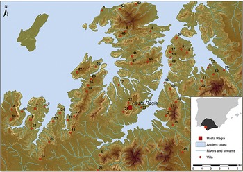
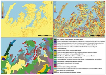
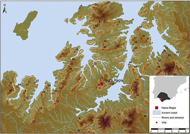
The present study builds upon prior field surveys and spatial analyses that have archaeologically documented the distribution of settlement across the study area. These foundational investigations have confirmed the presence and localization of various sites, forming the empirical basis for the current research. While the methodological details are further elaborated in the dedicated section of this work, it is important to note that the study area comprises a total of fifty-four Roman villas, which have been systematically selected for the application of the RBASE mid-range spatial model. These sites represent the core dataset for exploring patterns of land-use and spatial interaction, and their distribution is illustrated in Figure 1 and Table 1.
Area of study with Roman villa, and other geographical elements. A larger version of this figure is available to view at www.cambridge.org/spatial-analysis
1 Alventus
2 Berango I
3 Camino Monasterejos II
4 Carranza
5 Casa de Águila
6 Casa de la Gallarda
7 Caserón de Evorilla
8 Casita Palomares
9 Cerro Capita
10 Cerro Gibraltar
11 Corchitos 2
12 Corchitos 3
13 Cortijo de Alijar
14 Cortijo de Cestelo
15 Cortijo de Ébora 5
16 Cortijo de Monteagudo
17 El Pastor
18 Espartina
19 Finca el Olivillo
20 Haza de la Torre 2
21 La Galguera
22 Loma de Cartuja 3
23 Loma de Maina
24 Loma de Ventosilla
25 Loma del Alijar
26 Mojón Blanco II
27 Molino de Monteagudo 1
28 Monjas
29 Painobo
30 Portugalejo I
31 Portugalejo II
32 Pozos del Rosario
33 Regajo 1
34 Regajo 3
35 Viña Cabeza Alcaide
36 Viña de Arcade
37 Viña Rosario
38 Zarpa 2
39 Alamedinilla III
40 Casa del Hornillo
41 Casarejo 3
42 Cerro de las Vacas
43 Cerro de los Castillejos
44 Cortijo de la Fuente 1
45 Crespellina
46 El Cementerio
47 El Olivar Casarejo
48 El Peñón
49 El Pino 1
50 Loma de Espartina VIII
51 Mojón Blanco
52 Montegil de Buenavista1A/1B
53 Olivillo alto
54 Redondón
2 Theory and Research State
RBASE reinterprets classical spatial-economic models and replaces the isotropic logic of Euclidean buffers with functional accessibility. It models travel‐time/effort over friction surfaces to generate isochrones/isoergs, then sets these against fixed‐radius buffers to make the topographic deformation of space visible and measurable in each landscape. This tandem use clarifies what each approach captures and where it misleads.
Also, it is an update of SCA in the way of relating the sites with their surroundings. It was first defined by Vita-Finzi and Higgs (Reference Vita-Finzi and Higgs1970) as the analysis of archaeological sites in relation to their immediate environmental surroundings, with the aim of generating and testing hypotheses about past economies independently of excavated ecofacts; the classic operationalization used maximum daily exploitation radii of c. 10 km for hunting–gathering and 5 km for agriculture, expressed as two and one hours of walking to acknowledge topographic friction. The approach became especially influential in prehistoric studies (like early farming), and in 1972 the authors distinguished Site Territorial Analysis (STA), theoretical exploitation territories, from SCA in the strict sense, catchments of materials present in the deposit. RBASE differs by centering accessibility and mobility rather than only geometric distance: It couples concentric buffers with cost-surface‐based isochrones/isoergs (e.g., via Tobler’s walking function, Reference Tobler1993) and compares fixed-distance and fixed-time “near areas” at multiple scales within a documented, reproducible GIS workflow.
In the methodology section, further on, the changes and procedures are explained in detail. It is worth stating here, however, that Rbase is both new and distinct, as it introduces a straightforward approach that enables anyone to carry out this type of analysis. It employs multimodal distances incorporating rings and mechanisms to address overlaps, while also considering the intermediate space through nontheoretical ranges that aim to capture the practical distance of mobility, whether for undertaking specific tasks or for moving within a given society. This section critically assesses the limitations of traditional regional analyses and presents the conceptual framework of these spatial methodologies. It also situates the study within broader historiographical debates and explores the adaptation of Von Thünen’s model to archaeological analysis, other GIS applications, and the importance of the historical question that should always underlie our research.
2.1 The Limitations of Large-Scale Regional Analyses
A primary motivation underpinning this study stems from the critical observation that large-scale regional analyses frequently fail to capture the intricate complexities of local-scale interactions. This limitation becomes particularly apparent when examining production centers whose viability intrinsically depended upon the immediate environment for resource procurement. While traditional archaeological surveys and historical analyses have certainly succeeded in identifying broad distributional patterns of sites across the landscape, they often inadvertently overlook the significance of the micro-environment. Consequently, the crucial role played by localized geographic and ecological factors in shaping settlement patterns, resource management strategies, and agricultural practices frequently remains underexplored in macro-level investigations (Butzer, Reference Butzer1982).
A central methodological debate in archaeology lies in the dichotomy between on-site and off-site approaches: The former prioritizes excavation within clearly bounded locales such as settlements or cemeteries, focusing on stratigraphic depth, while the latter emphasizes surface survey techniques to capture dispersed material traces across broader landscapes, privileging spatial breadth. Although this distinction has shaped archaeological practice since the late twentieth century, it proves limited when confronted with contemporary landscape-based paradigms that move beyond predictive site identification to explore the interrelations of archaeological loci within political, economic, and social systems. These newer perspectives advocate abandoning rigid spatial binaries in favor of integrative frameworks that highlight continuity, interaction, and complexity in patterns of human occupation.
The critique of the on-site/off-site dichotomy was first articulated by Foley (Reference Foley1981a), who argued that the archaeological record should be understood as a continuous distribution of material remains across the landscape, with “sites” representing only peaks of artifact density within this continuum. Building on this reconceptualization, Bintliff in his influential paper The concepts of ‘site’ and ‘off-site’ archaeology in surface artefact survey (Reference Bintliff, Pasquinucci and Trement2000) emphasized that only through comprehensive mapping of all surface finds can archaeologists properly interpret the processes that generated them, rejecting the search for a fixed definition of settlement sites and highlighting that off-site zones are integral to the same continuum of human activity. His approach, exemplified in the Boeotia Survey, used intensive pedestrian survey and density mapping to analyze both site cores and surrounding low-density scatters, producing insights into land use, agricultural practices, and settlement intensity. In Off-Site Pottery Distributions (Bintliff and Snodgrass, Reference Bintliff and Snodgrass1988), the presence of extensive low-density ceramic carpets, linked to practices like waste disposal and manuring, further challenged rigid boundaries. Later surveys (Bintliff, Reference Bintliff2013, Reference Bintliff2023) confirmed that dispersed pottery fields are common, demonstrating that strict site/off-site distinctions obscure the multi-causal cultural, environmental, and taphonomic processes that structure archaeological landscapes.
Bintliff’s work aligns with a wider theoretical current in archaeology that questions the validity of the site concept, echoing early critiques by Schiffer (Reference Schiffer1972) and Dunnell (Reference Dunnell1971, Reference Dunnell1972), the latter together with Dunnell and Dancey (Reference Dunnell, Dancey and Schiffer1983) proposing the “siteless survey” as a method to document entire landscapes without assuming bounded sites. Rossignol (Reference Rossignol, Rossignol and Wandsnider1992) reinforced this position by showing how the fixation on sites neglects off-site materials, distorts data categorization, and oversimplifies human spatial practices, whereas artifact distributions, when freed from site-based assumptions, often appear as continuous gradients of land use. This reconceptualization shaped later work, such as Cherry et al. (Reference Cherry, Davis, Mantzourani, Cherry, Davis and Mantzourani1991), who pragmatically distinguished on-site and off-site data while recognizing them as parts of unified settlement systems, and Ebert (Reference Ebert1992), who argued for the outright abandonment of the site concept. Contemporary surveys often adopt hybrid approaches, recording dense concentrations (“feature clusters” or “site cores”) while also sampling the surrounding matrix, but all converge on the principle that fixed site boundaries must emerge from empirical artifact patterns rather than being imposed a priori.
Critics of the binary framework have emphasized its artificiality. David Pettegrew (Reference Pettegrew2001), for instance, criticized the tendency to classify dense artifact loci as farmsteads and all else as off-site, arguing that such distinctions obscure the full extent of habitation evidence. Drawing on ethnographic parallels, Pettegrew demonstrated that everyday discard practices generate low-density material scatters that are frequently indicative of habitation but are often misclassified due to their diffuse nature. Thus, archaeologists risk missing large portions of the occupation record by privileging only high-density clusters. Recent methodological guidelines have also reflected this critical stance. Attema et al. (Reference Attema, Bintliff and van Leusen2020), while still using the site/off-site terminology, emphasized the importance of careful, context-specific definitions. They introduced the concept of “site haloes” and “non-sites” to account for the broader spatial signatures of human activity, thereby moving toward a more integrated approach. Their work underscores that even projects that retain the language of “sites” increasingly acknowledge the complexity and continuity of artifact distributions beyond any core.
Current archaeology tends to treat sites as a heuristic, scale-dependent construct embedded in broader landscapes, distributions, and networks, with fuzzy boundaries that often reflect research design as much as past behavior. “Siteless” or distributional archaeology demonstrated that many artifact scatters form continuous surfaces punctuated by local density peaks; bounded sites are therefore one way, useful but partial, of slicing a spatial gradient (Foley, Reference Foley, Hodder, Isaac and Hammond1981b; Dunnell and Dancey, Reference Dunnell, Dancey and Schiffer1983; Ebert, Reference Ebert1992). Landscape archaeology reframed places as nodes within relational fields of movement, practice, and meaning, bringing attention to paths, vistas, affordances, and the historical co-production of people and environments (Tilley, Reference Tilley1994; Ingold, Reference Ingold1993; Ashmore and Knapp, Reference Ashmore and Knapp1999; David and Thomas, Reference David and Thomas2008). Methodologically, GIS-based approaches and spatial statistics operationalize this shift by mapping intensity surfaces, viewsheds, cost surfaces, and multi-scalar neighborhoods, thereby decentering rigid site perimeters in favor of gradients, connectivity, and accessibility (Conolly and Lake, Reference Conolly and Lake2006). In parallel, network analysis models interplace ties (movement, visibility, exchange), treating sites as vertices within multiscalar graphs and complementing distributional and landscape perspectives (Brughmans, Reference Brughmans2010; Knappett, Reference Knappett2011). Theoretical syntheses further argue that “site” is not a naturally given unit but a product of formation processes and analytical practice, which should be made explicit when defining study units and comparing cases (Lucas, Reference Lucas2012). Together these developments do not abolish the site concept; they contextualize and qualify it, encouraging analysts to choose units appropriate to questions and scales, to report boundary decisions transparently, and to integrate site-based evidence within distributional, landscape, and network frameworks.
Our main base for RBASE, SCA, designates a family of methods that relate archaeological sites to the environmental resources structuring subsistence by delimiting time–distance exploitation areas and, in the strict sense, by tracing the likely source areas of materials found in deposits; its classical formulation defined one-hour agricultural and two-hour hunting–gathering radii expressed as walking time, distinguished SCA from outward-looking STA, and used these tools to test claims about early agriculture (Vita-Finzi and Higgs, Reference Vita-Finzi and Higgs1970; Jarman, Vita-Finzi and Higgs, Reference Jarman, Vita-Finzi, Higgs, Ucko, Tringham and Dimbleby1972; Bailey, Reference Bailey, Renfrew and Bahn2005). Building on antecedents in economic geography and central-place reasoning, the approach sought independent hypotheses about economy and land use beyond artefact typology, while subsequent critiques clarified assumptions about site function, mobility, and environmental reconstruction (Chisholm, Reference Chisholm1962; Roper, Reference Roper1979; Bailey, Reference Bailey, Renfrew and Bahn2005). From the 1990s, GIS implementations replaced circular buffers with friction-aware catchments and made procedures more explicit and reproducible, while case-driven surveys continued to link catchment structure to agricultural resources, upland exploitation, and craft/material procurement, and later syntheses recapitulated SCA’s scope and limits and proposed geoarchaeological updates (Hillman, Reference Hillman1973; Simmons, Reference Simmons1975; Findlow and Ericson, Reference Findlow and Ericson1980; Hunt, Reference Hunt1992; Ducke et al., Reference Ducke, Kroefges, Rassmann, Posluschny, Lambers and Herzog2008; Dasgupta Ghosh, Reference Dasgupta Ghosh, Shinde, Raczek and Possehl2014; Volkmann, Reference Volkmann, Siart, Forbriger and Bubenzer2018).
On the other hand of the picture, we have the scholarly investigation of spatial relationships within historical and archaeological contexts, which has undergone significant methodological evolution over recent decades. This has led to the development of various models and analytical methods designed to better comprehend how human settlements interacted dynamically with their surrounding environments. As perceptively discussed by Conolly and Lake (Reference Conolly and Lake2006), earlier approaches predominantly relied upon relatively simple proximity analyses or expansive regional surveys. Complementing this, Fábrega Álvarez and Parcero Oubiña (Reference Fábrega Álvarez and Parcero Oubiña2007) propose a robust theoretical and methodological framework for the archaeological analysis of pathways and movement. While these methods proved effective in discerning general trends and patterns at a broad scale, they often lacked the resolution necessary to capture the localized interactions and site-specific dynamics that are fundamental to understanding the unique operational logic and historical trajectory of individual settlements or activity areas (Kvamme, Reference Kvamme1999).
In more recent years, substantial advancements in Geographic Information Systems (GIS) technology have fundamentally revolutionized archaeological spatial analysis, mainly with new tools or multi-scaler analysis (Howey, Reference Howey2007; Viitanen, Reference Viitanen2010; Mayoral et al., Reference Mayoral Herrera, Parcero-Oubiña and Fábrega-Álvarez2017). This technological shift has enabled the execution of far more sophisticated studies capable of integrating and interrogating multiple layers of geographic variables simultaneously. The work of M. Llobera (Reference Llobera2001), for instance, was instrumental in advocating for the adoption and application of GIS within archaeology, particularly highlighting its power in analysing visibility networks (viewsheds) and modeling potential movement pathways across landscapes. Indeed, the systematic consideration of factors such as visual prominence and the influence of topography on shaping human behavior, perception, and settlement location choices continues to be a cornerstone of contemporary spatial archaeology (Ashmore and Knapp, Reference Ashmore and Knapp1999).
Mobility analyses in archaeology and history investigate how sites relate to their environmental settings by converting terrain and infrastructural affordances into traversability, time–distance, and network models that articulate access, connectivity, and territorial maintenance (Conolly and Lake, Reference Conolly and Lake2006). Early practice coalesced around slope‐informed walking functions, above all Tobler’s hiking function, which grounded time budgets and cost surfaces for pedestrian movement (Tobler, Reference Tobler1993). The field has been theorized into coherent least-cost frameworks linking methodological choices to inferential claims and case design, consolidating both procedures and interpretive scope (White and Surface-Evans, Reference White and Surface-Evans2012). Authoritative reviews have systematized debates over anisotropy, friction parameters, and reproducibility, establishing cautions and good practice for comparative work (Herzog, Reference Herzog2014; Verhagen et al., Reference Verhagen, Nuninger, Groenhuijzen, Verhagen, Joyce and Groenhuijzen2019). A widely cited empirical application along the later prehistoric Ridgeway demonstrates how topography and cultural constraints interact with modeled paths and ground observations (Bell and Lock, Reference Bell, Lock and Lock2000b). Technically, approaches divide between isotropic cost surfaces that assume direction-independent frictions and anisotropic models that penalize ascent–descent and direction of travel, enabling more realistic pedestrian networks (White and Barber, Reference White and Barber2012). Beyond single “optimal” lines, circuit theory yields corridor-like solutions that represent multiple plausible routes under heterogeneous conditions (Howey, Reference Howey2011). Historical itinerary reconstruction further serves to validate and calibrate friction choices against documentary movement evidence (Seifried and Gardner, Reference Seifried and Gardner2019). Recent work introduces direction-independent travel budgets and ensemble modeling to express uncertainty and alternative behaviors in combined maritime–terrestrial contexts (Carroll et al., Reference Carroll2022).
Cost Surface Analysis, a powerful GIS technique, has emerged as a standard tool within the archaeological research toolkit. This methodology calculates the accumulated “cost,” often conceptualized as energy expenditure, time, or perceived difficulty, of traversing a digital representation of a landscape. This cost is typically determined by factors such as slope gradient, terrain type, or land cover. By modeling these costs, the method allows researchers to generate more nuanced and plausible reconstructions of past movement patterns, explicitly accounting for the physical challenges and constraints imposed by the terrain itself (Grau, Reference Grau2006). The versatility and utility of those cost analyses are demonstrated by their numerous relevant applications across diverse geographical and chronological contexts, ranging from prehistoric periods to modern historical landscapes (David and Thomas, Reference David and Thomas2008).
Cost surface analysis in GIS simulates effort-based travel across landscapes, incorporating variables such as slope, elevation, and hydrological constraints to identify routes of least resistance, routes that often align with what Roman engineers may have considered optimal (Fonte, Parcero-Oubiña, and Costa-García, Reference Fonte, Parcero-Oubiña and Costa-García2017; Carreras and Morer, Reference Carreras and Morer2014). This type of analysis allows researchers to infer how practical considerations of topography influenced infrastructure. For example, Verhagen et al. (Reference Verhagen, Nuninger, Groenhuijzen, Verhagen, Joyce and Groenhuijzen2019) explore the limitations of least-cost modeling and stress the importance of calibrating models using archaeological validation, highlighting how these tools can both illuminate and mislead if not critically assessed.
In contrast, network-based approaches model movement by treating mansiones or key settlements as nodes, and the routes connecting them as edges. These methods, inspired by graph theory and complexity science, emphasize accessibility, centrality, and redundancy within imperial logistics systems (Graham, Reference Graham2006; Isaksen, Reference Isaksen2008). By abstracting from the terrain, such models reveal patterns of communication and control that may not be visible in terrain-dependent reconstructions. Graham’s application of agent-based models to the Antonine Itineraries, for example, suggests Roman infrastructure was not only shaped by geography but also by political and administrative agendas.
Recent scholarship has sought to bridge these perspectives, advocating for hybrid models that integrate environmental data with network structures (Wheatley and Gillings, Reference Wheatley and Gillings2002; Herzog, Reference Herzog, Contreras, Farjas and Melero2013). Moreover, Llobera (Reference Llobera2000) and Bell and Lock (Reference Bell, Lock, Lock and Brown2000a) emphasize the experiential aspect of movement in ancient landscapes, arguing that path choices were not always about efficiency but were influenced by visibility, symbolism, and social practices. These considerations challenge the assumption that least-cost paths always reflect historical reality, reinforcing the value of interpretative pluralism in archaeological GIS. Argüelles-Álvarez and Trapero-Fernández (Reference Argüelles-Álvarez and Trapero-Fernández2025) exemplify this approach in their study of Roman road XIX in northwestern Iberia, combining GIS terrain modeling with itinerary data to refine our understanding of the rationality behind Roman route placement. This integrated method respects both the physical constraints of movement and the historical realities of Roman administration.
Ultimately, cost-path models and network analyses are not opposing strategies but complementary tools. While the former helps ground reconstructions in empirical, terrain-based evidence, the latter highlights the abstract logic of spatial governance and control. Together, they provide a multidimensional lens for understanding how Roman roads operated both as physical conduits and as instruments of imperial cohesion.
We can not forget visibility analyses that evaluate how sites relate to their surrounding landscapes by modeling fields of view, intervisibility, and horizon structure as historically consequential affordances rather than purely geometric properties (Wheatley, Reference Wheatley, Lock and Stancic1995). Foundational theoretical work integrated GIS line-of-sight with questions of perception, monumentality, and social practice, establishing a programmatic agenda for visibility studies (Wheatley and Gillings, Reference Wheatley, Gillings and Lock2000). A consolidated methodological synthesis then codified core procedures, parameters, and interpretive cautions for archaeological visibility (Wheatley and Gillings, Reference Wheatley and Gillings2002). The conceptual toolkit expanded from point-based viewsheds to “visualscapes” and “total viewshed” approaches that describe the inherent visual structure of landscapes (Llobera, Reference Llobera2003). Comprehensive reviews clarified debates over observer/target heights, DEM error, refraction, vegetation, and reproducibility, and recommended good practice for comparative research (Lake and Woodman, Reference Lake and Woodman2003). Technically, multi-viewshed workflows and horizon-aware calculations demonstrated how cumulative visibility patterns and skyline constraints reshape interpretations of signaling, surveillance, and monument placement (Ruggles, Medyckyj-Scott, and Gruffydd, Reference Ruggles, Medyckyj-Scott, Gruffydd, Andresen, Madsen and Scollar1993). Uncertainty has been formalized through fuzzy viewsheds to represent gradations in visibility and data error (Fisher, Reference Fisher1992). Subsequent extensions broadened applicability in planning and archaeology by generalizing viewshed computations and accounting for additional sources of variance (Fisher, Reference Fisher1996). Empirical tests within and beyond socio-political cores have linked visibility metrics to settlement hierarchies and territorial dynamics (Supernant and Prentiss, Reference Supernant and Prentiss2014). Route-based visibility further shifted attention from static vantage points to how visibility accumulates along movement corridors, improving inferences about wayfinding and experiential aspects of travel (Chamberlain and Meitner, Reference Chamberlain and Meitner2013).
We did not consider the use of visibility tools in this analysis with RBASE, primarily because, although they are indeed valuable for understanding the relationship between space and site, in the Roman-period context they do not constitute the decisive factor. Visibility is often associated with visual control and defensibility; however, in this case, the former may be applicable only insofar as it does not hinder or reduce the suitability of a location for the exploitation of resources, while the latter has only minimal influence.
The application of these GIS-based spatial analyses is currently expanding to encompass a broader range of research questions, extending beyond simple mobility to explore phenomena from economic perspectives (e.g., assessing land suitability for specific activities like viticulture (Trapero, Reference Trapero Fernández2021a) as well as investigating social dynamics and interaction spheres (White and Surface-Evans, Reference White and Surface-Evans2012). It is crucial to acknowledge, however, that these tools possess well-documented limitations. Principal among these are the common reliance on slope as the primary determinant of cost, the potential impact of choosing different cost-calculation algorithms, and the inherent requirement of defining discrete start and end points for pathfinding analyses, among other factors (Herzog, Reference Herzog2014). Despite these caveats, such tools are often employed with greater confidence and precision when the objective is to understand and reconstruct communication routes themselves, with a particularly strong and productive focus on Roman road networks in recent scholarship (Verhagen et al., Reference Verhagen, Nuninger, Groenhuijzen, Verhagen, Joyce and Groenhuijzen2019).
It is important to recognize, however, that the aforementioned approaches, particularly standard cost analyses, typically focus on modeling connectivity between different spaces or sites, rather than concentrating the analysis on the characteristics of a specific site and its immediate operational territory. The methodological development within this domain of GIS-based mobility studies has been considerable. It has progressed from foundational algorithms designed to transform movement potential into quantifiable data, often expressed in units of energy or time (Tobler, Reference Tobler1993), through critical engagement with the inherent methodological challenges and assumptions (Llobera, Reference Llobera and Sluckin2007), toward more integrated approaches capable of understanding mobility from multiple origins or incorporating varied behavioral logic (Llobera et al., Reference Llobera, Fábrega Álvarez and Parcero Oubiña2011). The current trajectory reflects a broadening scope, encompassing visions that analyze not only human mobility but also the movement potential or spatial logic of other elements or processes within the landscape (Verhagen et al., Reference Verhagen, Brughmans, Nuninger, Bertoncello, Romanowska, Flores, Papadopoulos and Chrysanthi2013; Verhagen, Reference Verhagen2018).
Despite important advances in modeling inter-site connectivity and large-scale landscape movement, there remains a methodological need to design analytical frameworks capable of integrating such techniques with detailed local-scale investigations that explicitly consider the immediate environs of archaeological sites. Much GIS-based research continues to privilege macro-spatial perspectives, thereby neglecting proximate geographical factors such as terrain, soil, or hydrological variations within a site’s catchment that were likely decisive in ancient resource exploitation, land use, and daily practices. The RBASE model responds to this need by systematically combining established Cost Surface Analysis methodologies with fine-grained examinations of areas directly surrounding sites, incorporating environmental parameters such as soil type, geological substrate, and detailed topography. Through this integration, the model provides a refined understanding of how ancient communities perceived and utilized their immediate landscapes for activities like agriculture and resource management, emphasizing the importance of rigorously incorporating local-scale data into spatial analysis. The deliberate use of detailed topographic data in tandem with mobility analysis allows for a more realistic, contextually grounded reconstruction of how landscape features structured settlement and behavior.
In addition, the RBASE framework directly confronts the limitations of earlier spatial models, which often relied on simple Euclidean distance-based analyses and abstract isotropic assumptions. By embedding calculations of energy expenditure and time costs, RBASE shifts the focus toward embodied, anisotropic considerations of accessibility and effort, reflecting more closely the practical realities of ancient mobility and resource use. This orientation is consistent with recent theoretical directions in archaeology that stress human agency, situated decision-making, and the active role of landscapes in shaping practices (Wheatley and Gillings, Reference Wheatley and Gillings2002; Renfrew and Bahn, Reference Renfrew and Bahn2012). Traditional tools such as Least Cost Path (LCP), SCA, and basic viewshed mapping frequently oversimplify human-landscape interactions, assuming uniform behavior while overlooking micro-environmental variability and the inconsistencies of legacy survey data. By contrast, RBASE integrates multi-layered environmental data at fine scales, exposing subtle gradients of land suitability and accessibility, challenging slope-based or linear travel cost models, and offering an effort-sensitive framework that better reflects the complexity of ancient spatial strategies.
2.2 Historiographical Position and Study From the Historical Question
From a historiographical perspective, scholarship on the relationship between archaeological sites, landscape, and territory has long been guided primarily by archaeological optics. Over the discipline’s history, especially from the nineteenth century onward, attention frequently centered on the material vestige, from portable artifacts to monumental discoveries ranging from Pompeii to present-day excavations. While foundational, this emphasis often sidelined broader questions of spatial context and human–environment interaction beyond the immediate site envelope.
A persistent challenge, despite major methodological and technological advances, is the tendency to prioritize archaeological contexts without anchoring analysis to a clearly articulated historical research problem (Hodder and Orton, Reference Hodder and Orton1976). The interpretative power of an archaeological investigation diminishes when it is not framed within a delimited historical period, a specific social formation, or a concrete problematic. If a historically grounded question does not direct spatial analysis, even rich archaeological evidence will struggle to yield robust historical insight.
In this section, a “historically grounded question” is defined as one that (a) is tied to a clearly delimited time slice and social formation; (b) specifies the actors and practices of interest (e.g., villa-based viticulture, mixed farming, livestock management); (c) derives explicit expectations from period sources and prior scholarship; and (d) translates those expectations into measurable spatial proxies. Practically, such a question is implemented as testable statements about how a given community structured daily mobility and land use within its immediately surrounding operational territory. RBASE gives this form by delimiting the chronological horizon; identifying relevant practices (e.g., cultivation, pasturage, resource collection); selecting proxies for those practices (e.g., soils, slope, aspect/orientation, hydrology, road/water access); and evaluating them through cost-distance analysis, isochrones, and multi-layer comparison at the local scale. Spatial analysis is thus driven by the historical problem rather than by technique alone, and the physical, technological, and cultural dimensions are specified before modeling begins.
A second clarification concerns the use of “mentalités” (prevailing mentalities, worldviews, cultural logics). Here, mentalité is not a blanket temporal essence; it functions as evidentiary shorthand for historically specific cultural and technical preferences hypothesized from textual, epigraphic, and archaeological sources and then treated as variables within the model. For example, agronomic authors furnish directional and microclimatic preferences for vine orientation in Baetica; these are not asserted as timeless or universal, but used to weight orientation and wind-exposure parameters where attested, and only for the period and region to which they plausibly apply. In this sense, “mentalité” is a bounded hypothesis about practice, rendered explicit and testable via spatial proxies (e.g., aspect classes, exposure to prevailing winds), not an essentializing claim about epochs.
A further challenge relates to the excessive technification of tools such as GIS. In numerous instances, GIS cartography has been used as a sophisticated visualization rather than as a vehicle for spatial inference and hypothesis testing. Even when deployed analytically, GIS can mislead if not disciplined by a well-formulated historical question that sets the relevant variables, scales, and procedures. Within this study, the role of historical analysis is therefore fundamental. The study of landscape and territory acquires explanatory force only when it proceeds from a clearly delineated context and recognizes the considerable variability of historical processes across time and space. Complementary evidence, literary or epigraphic, where available, can sharpen that context and improve the precision of spatial analysis, while acknowledging that reconstructions remain, by the nature of the evidence, bounded approximations.
Within this framework, three categories of factors structure the analysis. Physical factors provide the relatively constant environmental baseline conditions of any territory, geology, topography, hydrography (shaping water availability), soil composition (conditioning agricultural potential), and climatic parameters (affecting faunal and floral ranges). Technological factors encompass the repertoire of a given period, labor power (human or animal), implements, and knowledge (e.g., plough types, irrigation techniques, construction methods), that condition how resources are accessed, extracted, transformed, and at what scale landscapes are modified. Cultural factors, traditions, customs, social structures, and belief systems filter which resources are valued or permissible to exploit and how they are managed; past strategies often prioritized resilience, adaptation, and pragmatic exploitation within specific cultural and environmental contexts. These dimensions interact dynamically: Physical factors set the stage (bearing in mind that present conditions may differ from past ones); technological capabilities define what could be done; cultural logics clarify why certain practices were adopted, preferred, or avoided, thereby giving deeper meaning to settlement and land-use patterns.
The methodology centers on correlating modeled human mobility with the potential for exploiting natural resources, explicitly considering pedestrian movement and, where historically appropriate, transport aids such as pack animals (e.g., horses or mules) or wheeled carts. The primary focus is on resources pertinent to subsistence and economic activity, agriculture, pastoralism (livestock rearing), and other uses such as hunting (cynegetic resources) or forestry (timber and woodland products). The guiding questions are therefore multifaceted: Which specific resources were potentially available within a defined territory on the basis of its physical characteristics? How might those resources have been used across different periods, given technological and cultural conditions? What was their potential economic significance? And conversely, how was the landscape itself modified by cumulative human activity over time? Rather than confining inquiry to a purely archaeological question, this approach evaluates interacting factors and assesses how exploitation of the surrounding environment evolved through distinct historical periods.
Within this design, the archaeological context remains indispensable for ground-truthing and contextualizing model outputs. The presence of specific ceramic forms (e.g., amphorae) may indicate consumption and distribution of wine within a region; yet such evidence does not automatically imply local production, as products may have been imported. The comparative juxtaposition of spatial potentials and archaeological signals thus answers targeted questions and generates new hypotheses.
Several recurrent failure modes have been identified when GIS-based tools are deployed without adequate historical and contextual control. A first pattern is the inference of causal explanations from mere covariation between palaeoenvironmental proxies and cultural variables, often treating environmental thresholds as quasi-natural laws while under-specifying social mechanisms, alternative hypotheses, and scale compatibilities (Contreras, Reference Contreras2016; Arponen et al., Reference Arponen, Dörfler and Feeser2019). A second pattern is discursive: Broad narratives reduce complex social change to climate or environment, occluding institutional, economic, and cultural mediations through which stressors are experienced and acted upon (Hulme, Reference Hulme2011; Middleton, Reference Middleton2012). In both patterns, the model risks standing in for historical reasoning instead of being embedded within it. With respect to SCA-style approaches, failures typically arise when isotropic perimeters (e.g., circular buffers at fixed radii) are used as proxies for functional territories without testing anisotropy, seasonality, or return costs, and without aligning environmental maps to the chronological and technological conditions of the period under study. This invites circular, distance-driven reconstructions that neglect how mobility, labor, and land-use are shaped by topography and social practice (Conolly and Lake, Reference Conolly and Lake2006). Historiographical critiques likewise show that deterministic readings of environmental contexts, such as peatland settings or Holocene proxy sequences, can conflate coincidence and causality, underplay equifinality, and neglect uncertainty in temporal alignment (Coombes and Barber, Reference Coombes and Barber2005; Plunkett, Reference Plunkett2013). In LCP modeling, contextual failures stem from underspecified friction surfaces (e.g., slope-only cost with uniform walking speeds), omission of two-way travel and load effects, and neglect of seasonal hydrology or historically attested corridors; LCP paths are then taken as evidence of past movement rather than as hypotheses to be confronted with texts, surface archaeology, or logistics (Conolly and Lake, Reference Conolly and Lake2006). Comparable issues arise with viewshed analysis when bare-earth line-of-sight rasters are interpreted as social “visibility” without accounting for vegetation, atmospheric conditions, or the cultural meaning of seeing/being seen, again allowing tool output to substitute for contextual argument (Conolly and Lake, Reference Conolly and Lake2006).
Against this background, RBASE is designed to resist any collapse of spatial variability into abstract epochs. It does so in three complementary ways. First, it implements regional parameterization and local proxies: The model is calibrated with fine-grained environmental layers (soils, slope, hydrology, aspect) and historically grounded mobility ranges, and weights can be varied across micro-regions so that the same chronological horizon can yield different modeled operational territories in different places. Second, it employs a multi-scalar design: Analyses are run at multiple, nested scales (e.g., near-site rings at 100 m and 1,000 m alongside a 15-minute mobility neighborhood), and results are compared across those scales, capturing spatial heterogeneity within a single period rather than forcing a single epochal pattern. Third, it treats historically contingent cultural and technological factors as testable inputs rather than axioms: Labor regimes, transport aids, and cultivation choices are introduced where independently attested and evaluated against spatial evidence (distributional statistics, sensitivity tests); when such evidence is weak or absent, the model defaults to physical constraints rather than to cultural assumptions. More broadly, RBASE replaces distance-as-proxy with functional accessibility by generating anisotropic isochrones on friction surfaces and systematically juxtaposing them with fixed-distance buffers; the deformation of space by topography thus becomes explicit and measurable rather than assumed. It requires data curation and temporal/spatial alignment, Coordinate Reference System (CRS) harmonization, quality checks, explicit site-selection criteria, and frames results as hypotheses to be triangulated with archaeological and historical evidence, thereby operationalizing the consilience long urged in climate, society and environment, and culture research (Contreras, Reference Contreras2016; Haldon et al., Reference Haldon, Mordechai and Newfield2018). By foregrounding agency, heterogeneity, and landscape co-production, the approach is positioned to avoid environmental reductionism, aligning with case-based critiques that show how infrastructure, knowledge, and practice mediate environmental constraints (Erickson, Reference Erickson1999; Middleton, Reference Middleton2012).
Situated within the broader trajectory of spatial archaeology, from early SCA and cultural ecology to landscape approaches influenced by processual and post-processual currents, this project repositions GIS as a hypothesis-driven instrument of historical inquiry. Unlike traditional models emphasizing site distributions or territorial hierarchies, the focus here is the operational territory immediately surrounding a site: a micro-territory conceived not merely as physical space but as an interface shaped by daily practice, resource management, and ecological adaptation. By grounding the analysis in the concrete question of how ancient communities exploited their immediate environment for agricultural and economic activity, the model links environmental data to historically framed interpretation and remains attentive to the mentalities and logistical capacities of the societies under study.
One element not yet discussed, but important to consider, is the role of noninvasive technologies, which compel us to approach these studies from perspectives that extend beyond the simple determination of archaeological sites or the assessment of resource exploitation. Today, a wide array of techniques allows us to investigate and document sites without excavation, operating at scales that can range from the highly localized to very broad regional surveys. Nondestructive methods permit the acquisition of high-resolution data without physical intervention (Sarris, Reference Sarris2015). Remote sensing, classically aerial photography and, more recently, high-resolution drone and satellite imagery, documents features such as cropmarks, soil marks, and subtle topographic variations, enabling the detection of unknown sites and the delineation of boundaries, including seasonal and environmental dynamics (Gaffney and Gater, Reference Gaffney and Gater2003; Mayoral et al., Reference Mayoral Herrera, Parcero-Oubiña and Fábrega-Álvarez2017). Light Detection and Ranging (LiDAR) and 3D modeling produce highly accurate terrain representations and reconstructions that reveal terraces, ditches, hydraulic works, and road networks otherwise obscured by vegetation or modern overprints (Campana and Piro, Reference Campana and Piro2009; Doneus, Reference Doneus2013; Kokalj, Ž. and Hesse, Reference Kokalj and Hesse2017). Wide-area LiDAR in the tropics has shown that past human activity often appears as continuous or near-continuous terrain modification radiating from settlement nuclei, hydraulic systems, and causeways rather than as neatly bounded “sites,” with landmark syntheses at Caracol (Belize), northern Guatemala (>2,000 km²), Angkor (Cambodia), and the Llanos de Mojos (Bolivian Amazon) (Chase et al., Reference Chase, Chase and Weishampel2011; Evans et al., Reference Evans, Fletcher and Pottier2013; Canuto et al., Reference Canuto, Estrada-Belli and Garrison2018; Prümers et al., Reference Prümers, Jaimes Betancourt and Iriarte2022). Parallel theoretical and methodological critiques since the 1980s have urged archaeologists to treat the record as continuous distributions in which “sites” are density peaks, while intensive pedestrian survey and best-practice syntheses emphasize region-wide, artefact-level recording and transparent sampling (Foley, Reference Foley1981a; Dunnell and Dancey, Reference Dunnell, Dancey and Schiffer1983; Bintliff and Snodgrass, Reference Bintliff and Snodgrass1988; Pettegrew, Reference Pettegrew2001; Attema et al., Reference Attema, Bintliff and van Leusen2020). Practice, however, remains uneven: Where LiDAR or full-coverage survey exists, research design and interpretation routinely reflect multi-scalar processes beyond site boundaries, whereas elsewhere publication formats and inventories still default to site-first categories. Geophysical prospection (magnetometry, resistivity, ground-penetrating radar, conductivity) complements these approaches by detecting subsurface features without excavation (Conyers, Reference Conyers2013), but it typically operates at intra-site scales and requires integration with regional analyses. Within this landscape, RBASE bridges detection and environmental interpretation by embedding site-level signals within broader environmental frameworks (terrain, soils, hydrology) while relying on systematic surface survey to supply off-site distributions; intensive fieldwalking remains crucial for capturing diffuse artefact scatters and land-use indicators that geophysical tools often miss. A multiscalar synthesis, combining intra-site precision with catchment-scale modeling, underpins the reconstruction of human–environment interaction.
Beyond individual case studies, the project also presents a reproducible methodology: a clear workflow and set of analytical procedures adaptable to other regions, periods, or questions. One advantage is the capacity to analyze multiple sites simultaneously within a territorial framework, facilitating the identification of broader spatial patterns, functional relationships, and potential site hierarchies. The method is flexible and broadly applicable, provided it remains consistently guided by a robust and well-articulated historical question. The systematic integration of physical, technological, and cultural analyses yields a more holistic and historically contingent account of how human societies have interacted with, adapted to, and transformed their environments over time.
2.3 Spatial-Economic Foundations and the Adaptation of Von Thünen’s Model in Archaeological Analysis
One of the key theoretical contributions to the spatial understanding of land use and economic organization is Johann Heinrich von Thünen’s Location Theory, formulated in the early nineteenth century (Chisholm, Reference Chisholm1962). Although primarily conceived within the field of agricultural economics, this model has since permeated diverse domains, including geography, urban studies, and, more recently, archaeology. While its historical assumptions are theoretical, von Thünen’s model presents a compelling starting point for analyzing spatial relationships between productive activities and geographic distance. Its legacy informs not only our understanding of spatial logic but also provides a foundation that, when critically adapted, can enrich archaeological models such as RBASE.
At the heart of von Thünen’s theory lies the notion of an “isolated state,” a hypothetical, uniform plain with a single central market and consistent environmental conditions. Farmers within this state are assumed to act rationally, seeking to maximize profits. Given the transportation cost of moving goods from rural production zones to the central market, von Thünen posited that land-use intensity would diminish with distance. This dynamic would generate concentric zones of agricultural activity: From high-cost, perishable goods like dairy or vegetables near the center, to extensive, low-maintenance land uses like grain or livestock at the periphery (Peet, Reference Peet1998).
This spatial logic is formalized in von Thünen’s rent equation:
R = Y(P − C) − TD
Where:
R = Land rent
Y = Yield per unit
P = Market price
C = Production cost
T = Transportation cost per unit of distance
D = Distance from market
Despite its abstraction, this equation highlights the fundamental interplay between distance, productivity, and economic value, a relationship that remains analytically powerful. It established a clear conceptual framework for understanding how spatial variables affect decision-making in land exploitation.
However, the model has some limitations. Its assumptions about homogeneity (in terrain, soil fertility, market structure, and behavior) make it ill-suited to real-world conditions, let alone historical ones. The fixed central market, uniform environmental context, and neglect of political, technological, and cultural factors render the model overly static and economistic. These criticisms are particularly relevant for archaeological applications, where subsistence strategies are embedded in complex socio-environmental systems, and where markets, if present at all, functioned under different logics than those of modern capitalism.
Nonetheless, von Thünen’s core insight, that spatial distance and environmental constraints significantly shape economic behaviors, remains profoundly relevant. Modern variants have emerged to expand or modify his ideas:
Weber’s Industrial Location Theory introduces labor costs and agglomeration economies, offering a more flexible framework for understanding the geography of production (Weber, Reference Weber1929).
Christaller’s Central Place Theory, although primarily concerned with service distribution and settlement hierarchies, borrows von Thünen’s spatial logic to model optimal locations for goods and services (Christaller, Reference Christaller1933).
Building on Christaller, Lösch’s Economics of Location (Reference Lösch1940) sought to develop a more flexible and realistic model that accounted for both supply and demand dynamics. His theory incorporated production and consumption zones and permitted greater complexity in spatial arrangements. It imagines a landscape shaped by overlapping market areas, resulting in an adaptable but still geometrically informed network (Lösch, Reference Lösch1954)
Alonso’s Bid-Rent Theory adapts the rent gradient concept to urban contexts, where different land users compete for central locations based on their needs for accessibility (Alonso, Reference Alonso1964).
Spatial Computable General Equilibrium models are new and more reliable models for land use and transportation that simulate interregional economic interactions and include spatial frictions and transportation costs that echo von Thünen’s principle (Anas and Liu, Reference Anas and Liu2007).
These developments illustrate the enduring power of the spatial-economic paradigm initiated by von Thünen. However, in history these principles require reinterpretation. Rather than adopting von Thünen’s assumptions wholesale, RBASE uses them as a conceptual scaffold, modified to reflect the historical and environmental specificity of past landscapes.
Unlike von Thünen’s economic model, which assumes a central market and profit-maximizing behavior, the RBASE framework prioritizes accessibility, mobility, and effort as the primary variables in land-use organization, generating isochrones and isoergs based on real topographic data rather than concentric rent zones. By modeling functional accessibility instead of monetary value, RBASE incorporates terrain, soil, and orientation into buffer zones around sites to determine plausible activities such as farming, grazing, or resource collection. It also replaces abstract distance units with historically grounded proxies, such as the Roman centuria system and realistic round-trip mobility rings of 15–30 minutes, thus capturing human-landscape interaction with greater precision than Euclidean measures. Finally, RBASE recognizes that land-use decisions were informed not only by economics but also by cultural, technological, and social factors, such as labor supply, agricultural traditions, and environmental perception, reflecting embedded, context-specific strategies of precapitalist societies (Forbes, Reference Forbes1993).
They share key assumptions that RBASE reinterprets, as with SCA analysis, so we compare the main dimensions in Table 2:
| Dimension | Classical SCA | RBASE (historically informed mode of application) | Spatial-economic models (von Thünen, Christaller, Alonso, Weber, Lösch, SCGE) |
|---|---|---|---|
| Ontological status | Method with a toolkit (buffers, catchments, cost surfaces) often applied generically | Mode of application: a procedural framework that governs how SCA tools are configured and interpreted in light of period evidence; not an algorithm | Abstract economic theories with formalized assumptions and equations |
| Positioning (vision) | Site-centered analysis of near environments | Intermediate: Site-centered but explicitly tied to historically delimited communities, practices, and periods; bridges SCA and spatial-economic logics | Market- and hierarchy-centered views (rings, bid-rent gradients, central places) |
| Historical grounding | Often limited periodization; weak linkage to sources | Strong: Defines a historically grounded question; derives expectations from texts/epigraphy/archaeology; encodes them as spatial proxies and parameters | Stylized epochs; history enters mainly via parameter tweaks or comparative statics |
| Market assumption | None required, sometimes implicit | None required; works without central markets; models access/effort rather than prices/rents | Central market or service hierarchies typically assumed; monetary rent central |
| Dimension | Classical SCA | RBASE (historically informed mode of application) | Spatial-economic models (von Thünen, Christaller, Alonso, Weber, Lösch, SCGE) |
|---|---|---|---|
| Mobility and cost | Euclidean buffers or generic cost surfaces | Anisotropic friction (slope, hydrology, aspect), isochrones/isoergs (time/effort); comparison with fixed buffers to expose spatial deformation | Transport cost typically abstracted; homogeneous planes common |
| Environmental heterogeneity | Physical layers used but often uniformly weighted | Region-specific weighting and micro-regional parameterization (soils, slope, orientation, water, route access) | Frequently homogeneous space or simplified gradients |
| Cultural and technological factors | Sometimes noted qualitatively | Operationalized as adjustable parameters when attested (labor regimes, transport aids, cultivation choices); defaults to physical constraints when evidence is weak | Usually exogenous to the model’s core mechanics |
| Temporal design | Single snapshot or broad phase | Time-sliced runs by period; historically grounded mobility ranges; explicit comparison across periods | Often atemporal or equilibrium-focused |
| Noninvasive data integration | Used ad hoc (e.g., LiDAR as terrain) | Bridges detection and interpretation: Integrates LiDAR/RS/geophysics with environmental modeling; complemented by systematic surface survey for off-site signal | Not specified in original formulations |
| Dimension | Classical SCA | RBASE (historically informed mode of application) | Spatial-economic models (von Thünen, Christaller, Alonso, Weber, Lösch, SCGE) |
|---|---|---|---|
| Scale strategy | One or few catchment radii | Multiscalar: Near-site rings (e.g., 100−1,000 m) tested against 15−30 minutes mobility neighborhoods; cross-site synthesis | Scale implied by theory (rings, hexagons, bid-rent curves) |
| Validation and inference | Map-led interpretation; limited testing | Hypothesis-driven: Outputs treated as testable; triangulation with ceramics, survey, texts; sensitivity and distributional statistics | Theoretical fit/intuition; empirical validation external |
| Data curation and reproducibility | Varies; often under-specified | Enforced: CRS harmonization, quality checks, explicit site selection; documented, reusable workflow | Not addressed (theory-level) |
| Typical outputs | Catchments, least-cost paths, suitability maps | Operational territories (anisotropic isochrones), deformation diagnostics (buffers vs. isochrones), period-specific accessibility maps, scenario comparisons | Rings, gradients, hexagonal market areas, rent curves |
The theoretical legacy of von Thünen remains vital for spatial thinking in archaeology, but its full potential is realized only through critical adaptation. RBASE exemplifies such an adaptation, using distance, effort, and landscape logic not to explain profit-maximizing behavior, but to reconstruct how ancient people navigated and organized their environment in ways that were materially constrained, historically contingent, and culturally meaningful.
From a methodological standpoint, modern tools like GIS allow researchers to operationalize many of those spatial concepts in far more complex and geographically accurate ways. For example, GIS-based friction maps replace abstract transport costs with real landscape resistances; land suitability models substitute generalized soil fertility with classified, data-driven indicators of agricultural viability. This level of detail transforms the model from a theoretical abstraction to a spatial hypothesis testing tool, like emphasize visual and experimental factors in spatial analysis (Llobera, Reference Llobera2001), explore cost surfaces, catchment analysis and probabilistic models (Verhagen et al. 2012, Reference Verhagen, Nuninger, Groenhuijzen, Verhagen, Joyce and Groenhuijzen2019), interpretate emptiness of the landscape (Wheatley and Gillings, Reference Wheatley and Gillings2002) o calculating movement reflecting both economic and non economic constrains (Lake and Woodman, Reference Lake and Woodman2003), among other relevante methods and case studied.
RBASE sits within this growing tradition, combining economic geography’s analytical rigor with archaeology’s contextual depth. By adapting von Thünen’s foundational concepts to model spatial effort, not market proximity, and by integrating environmental data rather than assuming homogeneity, it transforms a classical model into a flexible archaeological methodology. It does not reject spatial-economic theory but reconfigures it to better reflect the physical and social realities of past human landscapes. In sum, RBASE should be understood as both a descendant and a critical reconfiguration of classic spatial-economic theories. It preserves the analytic clarity of these models, especially in emphasizing spatial logic and structural patterning, while also correcting for their ahistoricism, environmental abstraction, and market-centric assumptions. It demonstrates how a refined archaeological methodology can draw on economic geography while advancing its own theoretical and empirical contributions to the study of past landscapes.
3 Methodology
RBASE adopts a systematic multiscalar design in which the definition of candidate spatial ranges, both distance-based and time/effort-based mobility neighborhoods, is itself a core step of the methodology. Thresholds are justified empirically through data density and overlap behavior, and the choice of scale is evaluated with statistics on environmental variables to determine whether distance or time stabilizes patterns more effectively (e.g., soils). The framework integrates multiple environmental layers (slope, aspect, soils) within a single analytical apparatus and, where appropriate, combined suitability models, replacing single-factor proximity with a multidimensional view of near-site land-use potential. A standardized, reproducible pipeline, data curation, CRS harmonization, quality checks, and explicit site-selection criteria preceding cost modeling and zonal analyses ensure interoperability and interpretability across platforms (ArcGIS/QGIS/GRASS) (see Appendix, Table 7). It is transparent about algorithmic sensitivity in cost analyses (e.g., under Tobler-type walking functions) and therefore recommends combining travel-cost and cost-allocation outputs and intersecting their polygons to delimit influence areas that respect both time thresholds and topographic partitions. By bridging buffer analysis with topographic mobility, the model recentres inquiry on local decision spaces while remaining scalable, and operationalizes a nondestructive, GIS-based approach that links historical questions to transparent spatial proxies and documented workflows; appendices and tool notes secure methodological clarity and replicability.
This orientation is consistent with prominent trajectories in archaeological and historical research that emphasize human agency, situated decision-making, and landscapes as actively perceived and shaped by practice (Wheatley and Gillings, Reference Wheatley and Gillings2002). Conceived as a methodological framework to analyze the spatial relationship between a site and its immediate operational surroundings through an integrated multiscalar approach, it systematically combines GIS capabilities, targeted statistical analyses, and cost-surface modeling to quantify key environmental parameters in the proximate landscape. The section is organized around four axes: (a) foundational materials for model construction (data curation, acquisition of geographic information, and GIS implementation) articulated in accessible terms; (b) core operational components, distinguishing variants that apply linear versus topographic relationships; (c) strategies for integrating diverse spatial information to support specific analytical objectives; and (d) a self-critical appraisal of spatial and temporal handling, setting out assumptions and limitations together with practical avenues to mitigate or transcend them.
3.1 Materials: Data Foundations for Spatial Analysis
The successful execution of this study necessitates a diverse and rigorously curated corpus of materials, enabling both the precise geospatial localization of archaeological sites and their subsequent in-depth spatial analysis. This section does not introduce novel concepts, but is dedicated to defining the necessary materials and outlining the basic procedures required to ensure reproducibility. This corpus encompasses primary archaeological data alongside a suite of geographic information layers processed and managed within a GIS environment. Paramount importance has been placed on ensuring the quality, consistency, and methodological transparency of all datasets employed. This involved critical assessment of data provenance, the criteria underlying any existing classifications, and the original data acquisition methodologies, consciously seeking to mitigate potential biases and errors that could propagate into the final interpretations.
The core dataset of archaeological site locations was built through targeted field surveys and a historiographically informed review of published and archival sources, including only sites with verifiable geographic coordinates confirmed by direct observation or consistent prior documentation. Given the inconsistencies of legacy data and shifting classification conventions, a rigorous re-evaluation was conducted to correct errors, such as the frequent mislabeling of rural structures as “villas,” which risks distorting interpretations of settlement hierarchies and territorial organization.
To address these intrinsic inconsistencies and ensure a robust analytical foundation, a systematic data validation and refinement protocol was implemented, comprising several key stages:
Verification of Classification Criteria: A thorough assessment was conducted to determine whether sites recorded in previous literature were categorized according to standardized, explicit criteria, or if significant variations existed between different authors or survey projects. Where necessary and feasible, re-classification based on consistent criteria was performed.
Elimination of Redundancies and Duplicates: Careful cross-referencing was employed to identify and resolve instances where previous studies might have recorded spatially proximate find concentrations or structural remains as distinct sites, when archaeological evidence suggests they likely formed part of a single, larger functional unit (Grau, Reference Grau2017).
Critical Review of Legacy Data Provenance: Particular attention was paid to understanding the original survey methodologies employed in generating legacy datasets. Recognizing that different researchers may apply disparate criteria regarding survey intensity, collection strategies, and minimum thresholds for site definition, contrasting the validity and comparability of data derived from varying methodological origins was essential prior to integration.
One of the most pervasive challenges in landscape archaeology remains the lack of uniformity in defining the spatial extent or boundary of archaeological sites. Some surveys conceptualize a site as a singular point representing a primary concentration of materials, while others adopt a more granular approach, subdividing larger scatters or complexes into multiple closely spaced loci. For the present study, a methodological decision was made to maintain sites as distinct entities whenever the available archaeological evidence permitted differentiation based on spatial separation or functional interpretation. This approach, while demanding careful justification on a case-by-case basis, was deemed analytically advantageous. It facilitates a more nuanced examination of peripheral spaces and allows for the evaluation of whether specific material concentrations represent outliers of a central nucleus or potentially constitute distinct satellite activity areas possessing their own localized dynamics and catchment interactions.
The geographical datasets integrated into this study need to be meticulously selected based on their direct relevance to the core objectives of spatial modeling, particularly concerning the interplay between archaeological sites and their embedding environmental matrix. The primary datasets utilized include Digital Elevation Models (DEMs), various vector layers representing discrete landscape features, and raster datasets characterizing environmental variables.
Digital Elevation Model (DEM): The DEM serves as the fundamental topographic substrate for virtually all subsequent spatial analyses, providing detailed quantitative information regarding terrain morphology (elevation, slope, aspect, curvature) and enabling the application of sophisticated mobility, accessibility, and visibility models. The resolution of the DEM was strategically adjusted contingent upon the analytical scale:
◦ For broad regional analyses encompassing areas of several tens of square kilometers, a DEM with a grid resolution of 25 m was employed. This resolution was determined to offer an optimal balance between capturing significant topographic variation relevant at this scale and maintaining computational feasibility for complex geoprocessing tasks like cost surface generation.
◦ In specific sub-regional sectors or site-proximate zones demanding finer-grained analysis (e.g., detailed catchment modeling), higher-resolution DEMs (e.g., 5 m or derived from LiDAR where available) were utilized, provided data availability and quality permitted.
◦ Crucially, the quality of the source DEMs was rigorously assessed to ensure accurate representation of the terrain’s characteristics, actively identifying and mitigating potential distortions arising from excessive interpolation artifacts or the use of resolutions inappropriate for the scale of inquiry.
Complementary Geographic Vector Layers: A suite of vector layers was incorporated to effectively contextualize the archaeological sites within their broader natural and anthropogenic landscape framework. These layers included:
◦ Hydrography: Digitized representations of principal river courses, associated floodplain extents where reconstructable, and known or inferred intermittent streams (arroyos), critical for understanding water access, potential flood risks, and constraints on movement (Trapero, Reference Trapero Fernández2021b).
◦ Topography and Relief: Vector representations of significant geomorphological features (e.g., ridgelines, distinct geological formations) complement the DEM data.
◦ Historical Infrastructure: Documented or archaeologically attested ancient road networks, paths, or other communication routes relevant to the study period, providing known connectivity vectors.
◦ Settlements and Strategic Locations: Geospatial locations of known contemporary urban centers, ports, potential resource extraction sites, or other key nodes of human occupation influencing regional dynamics. The selection of these layers prioritized features exhibiting considerable temporal stability or whose historical modification over time could be reasonably traced or modeled, thus minimizing anachronistic projections onto the past landscape.
Environmental and Land Use Raster Data: Beyond the structural geographic data, raster layers conveying information about environmental characteristics were integrated, including:
◦ Soil Types and Edaphology: Data derived from soil surveys, crucial for evaluating the agricultural potential and constraints of terrains surrounding archaeological sites.
◦ Geology: Information on underlying geological formations, relevant for understanding potential raw material sources (e.g., clay, stone) and potential influences on hydrology and soil formation.
◦ Modern Land Use/Land Cover: Datasets derived from contemporary remote sensing or environmental databases (e.g., CORINE Land Cover), used cautiously primarily to identify areas of significant recent landscape transformation (e.g., modern urbanization, large-scale agriculture, reforestation) that might obscure or bias the interpretation of past land use potentials. It must be explicitly acknowledged that many readily available environmental datasets (particularly soil and geological maps) often possess inherent resolution limitations or generalizations that may not be ideally suited for highly detailed, micro-regional studies. Consequently, a preliminary critical evaluation was conducted for each dataset to ascertain whether its scale and accuracy permitted meaningful interpretation within the specific context and analytical requirements of the study area.
Following the precise delineation of the study area, the subsequent phase involves the meticulous acquisition of geospatial data essential for comprehensive analysis. This process encompasses the procurement of data pertaining to soil types, geological formations, topographic attributes, and other relevant environmental parameters. In the context of Colonia Hasta Regia, these data sets have been derived from a diverse array of sources, including geological surveys, historical soil maps, and high-resolution topographic models generated from LiDAR data. These disparate data are then integrated and processed using advanced GIS software to generate detailed spatial layers.
For instance, pedological data, extracted from studies that classify soils according to their agricultural potential during the Roman period, enable us to assess the suitability of various areas for cultivation. This evaluation is predicated on the soil’s capacity for moisture and nutrient retention, factors that were paramount for ancient agricultural practices. Furthermore, the generation of slope maps from topographic information is indispensable for identifying areas with significant traversal difficulties. These areas, which would have presented natural barriers, are critical for cost surface analysis and the reconstruction of mobility patterns (Carreras and de Soto, Reference Carreras and de Soto Cañamares2009).
In creating these models, archaeological data must be combined with environmental variables such as orientation, slope, and soil type, requiring a structured methodology of classification aligned with research objectives. Some data, like orientation values from DEMs, may not need reclassification for general analysis, but others, such as slope, demand it from the outset. Since slope values range continuously from 0° to 90°, often with decimals, the raw dataset can become overly complex; thus, grouping them into broader intervals (e.g., 1° or 2° Categories) provides a more manageable and analytically meaningful structure.
Similarly, in other spatial datasets, such as soil classifications or analogous environmental attributes, it is crucial to consider the symbology and classification system to be used as a reference. Since spatial analyses typically generate numerical outputs, maintaining a clear correlation between these numerical values and their corresponding textual classifications is essential. This ensures that the results remain interpretable and meaningful within the broader archaeological and environmental context.
Within the analytical framework focusing on spatial cost modeling and the delineation of site catchments or influence areas, GIS tools function as fundamental materials for the reconstruction, simulation, and interrogation of archaeological landscape scenarios. The following provides a technical overview of the principal geoprocessing tools and algorithms employed, referencing their implementation within common GIS software environments (QGIS, ArcGIS Desktop/ArcPro), tailored for a specialist audience familiar with these platforms.
Vector Entity Modification and Analysis:
◦ Buffers: Standard isotropic buffer generation was utilized for preliminary definitions of proximity zones around sites, useful for initial area-based queries or defining search radii. Advanced options for dissolving overlapping buffers or segmenting by attributes were employed as needed via tools available in QGIS (native or via plugins) and ArcGIS Spatial Analyst.
◦ Thiessen Polygons (Voronoi Diagrams): These were generated to partition space based on nearest-neighbor principles, providing theoretical territories of influence around point locations (sites). Implementations in QGIS (native or via Processing toolbox algorithms like GRASS v.voronoi) and ArcGIS (“Create Thiessen Polygons” tool) were used for exploratory spatial distribution analysis and potential hierarchy assessment.
Vector-Raster Format Conversion: The essential interoperability between vector (discrete object) and raster (continuous field) data formats is critical for integrating categorical landscape features with continuous environmental models, particularly for cost surface analysis.
◦ Vector to Raster Conversion: Polygon features (e.g., land use patches, specific soil types) were rasterized to align with the DEM grid structure, enabling their incorporation into friction surface calculations. Standard tools in QGIS (e.g., r.rasterize in GRASS, native algorithms) and ArcGIS (“Polygon to Raster”) were used, carefully controlling cell assignment rules and output resolution.
◦ Raster to Vector Conversion: The inverse process was employed to convert raster outputs (e.g., classified cost surfaces, delineated catchments) into vector polygons, facilitating area calculations, overlay analyses, and clearer cartographic representation of modeled zones.
Cost Distance Analysis and Associated Tools: This suite of tools forms the core of the accessibility modeling, simulating landscape “friction” or impedance to movement by integrating diverse physical, environmental, and potentially technological or cultural variables (Haisman and Goldman, Reference Haisman and Goldman1974):
◦ Core Cost Algorithms (Cost Distance, Cost Allocation, Cost Backlink): These foundational tools calculate the cumulative cost of movement from source locations across a friction surface, assign each grid cell to its least-cost source, and determine the direction of least-cost paths back to sources, respectively. Implementations within ArcGIS Spatial Analyst (“Cost Distance,” “Cost Allocation,” “Cost Back Link”) are standard. Equivalent functionalities were achieved in QGIS primarily through the integration of GRASS GIS modules (e.g., r.cost, r.walk for anisotropic costing) and SAGA GIS tools available via the Processing toolbox.
◦ Friction Surface Creation: The generation of a meaningful friction raster is a critical preparatory step. This involved reclassifying input rasters (e.g., slope derived from DEM, land cover types) into impedance values and often combining multiple reclassified layers using weighted overlays (via “Raster Calculator” in ArcGIS/QGIS or r.mapcalc in GRASS) to create a composite surface reflecting the combined difficulty of traversing different landscape conditions. Sensitivity analysis regarding friction value assignments is recognized as an important, though often complex, aspect of robust modeling.
◦ Complementary Cost Modeling Tools: Where appropriate, more advanced tools were considered:
◾ Path Distance (ArcGIS): Allows for the incorporation of additional cost factors beyond simple surface friction, such as horizontal or vertical movement constraints (e.g., simulating fatigue or slope-dependent effort), offering potentially more realistic movement simulations.
◾ Network Analyst (ArcGIS): Employed specifically when analysing movement constrained to predefined linear networks (e.g., reconstructing travel times along known Roman roads).
◾ Surface Hydrology Tools: Standard tools for deriving flow direction, flow accumulation, and watershed delineation were used to understand the influence of drainage patterns on landscape structure and potential movement corridors or barriers.
3.2 General RBASE Method
Within the broader field of archaeological spatial analysis, formally defining the site’s immediate sphere of influence or “near area,” the zone most intimately linked to its daily operations and resource procurement, “near area,” is a fundamental requirement. Methodologically, RBASE considers two principal, complementary approaches to delineating this critical proximal zone, as can be seen in Figure 2:
1. Defining Proximal Zones via Geometric Constructs: This approach relies on predefined shapes to establish the initial analytical boundaries.
◦ Polygons Based on Documented Territorial Divisions: In exceptional circumstances where detailed historical or archaeological evidence reveals specific, known land divisions directly associated with a site (e.g., clearly identifiable boundaries of a centuriated plot linked to a specific villa), these historically attested polygons can serve directly as high-fidelity analytical units. This method offers the distinct advantage of potentially reflecting actual administrative, economic, or property limits with considerable accuracy, though such detailed evidence is rarely available.
◦ Concentric Circular Buffers: In the more common absence of clearly defined ancient territorial boundaries, the generation of circular zones based on fixed radii from the site’s center provides a pragmatic and standardized alternative. As employed in the initial RBASE step described previously, this method is computationally straightforward and facilitates direct comparison between different sites based on simple proximity to resources or features. However, its inherent limitation lies in its isotropic assumption; it inherently ignores the profound influence of terrain relief and landscape friction on actual accessibility and movement patterns.
2. Defining Proximal Zones via Topographic and Cost-Distance Analysis: To overcome the significant limitations of purely geometric methods, RBASE heavily incorporates accessibility modeling based on cost-distance principles. This approach evaluates the effective effort required to traverse the landscape, thereby generating a more realistic model of functional proximity. The methodology centers on generating isochrones (contours connecting points reachable within equal travel time) or isoergs (contours of equal energy expenditure) emanating from the archaeological site. This is achieved by:
◦ Creating a friction surface (as described previously) that assigns impedance values to each grid cell based on variables significantly affecting movement effort, primarily slope steepness, but potentially also incorporating factors like dense vegetation cover or the presence of water bodies acting as barriers or corridors.
◦ Applying specific GIS algorithms, notably Cost Distance Analysis suites (e.g., ArcGIS Spatial Analyst’s Cost Distance/Cost Allocation or GRASS GIS’s r.cost/r.walk) and potentially LCP computations. These algorithms calculate the cumulative cost (in time or energy units) to reach every location in the surrounding landscape from the source site, effectively warping geographic space according to traversal difficulty. The resulting output is typically a spatially irregular, anisotropic zone representing the area realistically accessible from the site within a given effort threshold. This provides a functionally more meaningful representation of the territory likely most influential in shaping land-use decisions and resource exploitation strategies tied to the site.
Graphical explanation about the difference of both models.
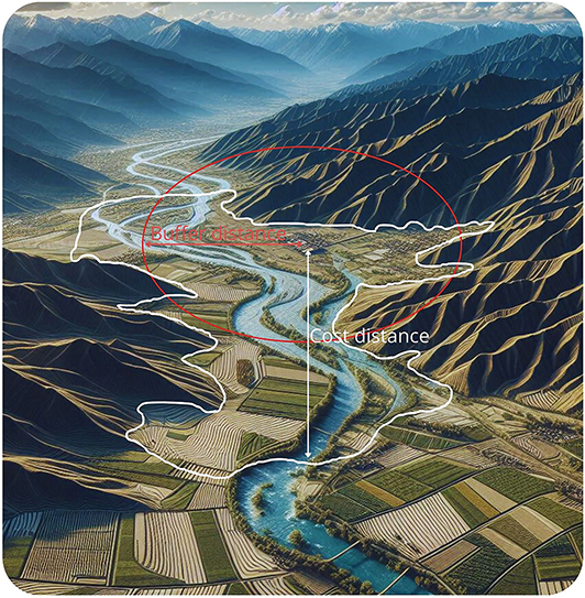
Crucially, the RBASE framework advocates for the synergistic use, rather than mutually exclusive selection, of these approaches. By generating both geometric buffer zones (grounded in historical scale proxies where possible) and effort-based accessibility zones (isochrones/isoergs), a more comprehensive and critically informed understanding of the site’s territorial context can be achieved. Comparing the spatial configuration and extent of fixed-radius buffers against the often highly irregular shapes of cost-derived zones allows researchers to explicitly visualize the impact of topography on accessibility, evaluate the validity and limitations of each method within the specific landscape context, and ultimately develop more nuanced interpretations of past spatial behavior and land management practices.
Table 3 outlines the conceptual and technical distinctions between buffer-based and cost surface models. While buffer models rely on uniform Euclidean distances for spatial analysis, cost surface models incorporate heterogeneous travel resistance, offering greater realism in complex terrains. Their respective tool requirements and performance implications reflect these methodological differences.
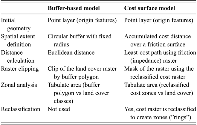
Table 3 Long description
Table 3 presents a structured comparison between buffer-based models and cost surface models, emphasizing their conceptual foundations and technical implementation. Both approaches begin with point geometries serving as origin features, yet they diverge in how spatial extent and distance are defined. Buffer-based models generate a circular area using a fixed Euclidean radius, applying uniform distance assumptions across the landscape. In contrast, cost surface models determine spatial reach through accumulated cost values derived from a friction raster, which accounts for heterogeneous travel resistance. This distinction extends to their analytical procedures: buffer models clip the land-cover raster using the buffer polygon, whereas cost surface models apply a raster mask based on reclassified cost values. Zonal analysis in the buffer approach evaluates land-cover classes within the circular polygon, while the cost surface model conducts the same operation on zones created from reclassified cost intervals. Reclassification is therefore a necessary step only in cost surface modelling, where it defines discrete cost “rings” for subsequent analysis. These methodological differences encapsulate the contrasting assumptions and analytical capacities of the two model types.
Each model is explained in detail in Table 3. For the correct reproducibility of the same, I add in appendix, six data sets with python, three for each model, to be applied in Arcpro, Arcgis, and Qgis.
RBASE contrasts two methods for defining a site’s territory: Isotropic geometric buffers (fixed or historically informed radii) and anisotropic isochrones from cost-distance surfaces. Buffers provide fast, transparent baselines, while isochrones account for real movement constraints, distorting rings around slopes, marshes, roads, or corridors. To make method choice explicit and reproducible, the study matches buffers and isochrones by area or time, then compares them through indices of overlap (intersection-over-union), environmental divergence (soil, slope, aspect differences), suitability capture (top-quartile cells), and land-use allocation shifts (Groups 1–3). Scale is empirically tested, with spatial ranges evaluated statistically to identify stable neighborhoods. The workflow integrates slope, aspect, soils, and combined suitability models within a reproducible pipeline (data curation, CRS harmonization, cost modeling, zonal analysis), while accounting for algorithmic sensitivities by reporting both travel-cost and allocation outputs and intersecting polygons to delimit realistic catchments. This bridges simple buffers with topographic mobility, grounding analysis in local decision spaces but retaining scalability and transparency.
Results show method and scale strongly affect interpretations: In heterogeneous or constrained terrain, isochrones warped by topography or hydrology can invert soil profiles implied by buffers, alter dominant land-use groups, shift suitability rankings, or bias sites near thresholds like marshes or palaeochannels. In open, homogeneous areas, buffers and isochrones converge, with high overlap and minimal divergence. At the regional level (e.g., fifty-four villas at Hasta Regia), differences matter when they change land-use dominance or suitability order. Accordingly, isochrones are adopted as the default catchment, with buffers as baseline comparators, and results reported through paired comparisons (buffer/isochrone parameters, overlap, composition divergence, suitability capture, land-use allocation, and direction of change), summarized at both site and sample levels with medians and interquartile ranges.
3.2.1 Buffer Model
As previously argued, in developing a buffer model, there are two primary approaches that can be employed. The first, and most straightforward, involves using a simple buffer technique. This method begins with the computation of mean distances via point distance calculation tools. The purpose of calculating the mean distance is to reduce the impact of outlier values and to establish a representative average distance, which then informs the selection of an appropriate buffer range. Ideally, buffers are generated using a fixed distance, for example, a standardized centuria distance, to maintain consistency across the analysis. However, when dealing with extensive areas, a fixed-distance approach may lead to overlapping buffers, thereby obscuring the true spatial boundaries (Partovi and Davison, Reference Partovi Nia and Davison2012).
The practical application of the RBASE framework begins with a crucial first step: The systematic delimitation of the analytical study area immediately surrounding the archaeological site(s) of interest. This is initially achieved through the generation of a series of nested, concentric buffer zones established at distinct, theoretically informed distances from the site’s defined center or extent. These buffer zones serve not merely as geometric constructs but function as primary spatial containers, facilitating the extraction, quantification, and comparative analysis of underlying geospatial data layers pertinent to environmental characterization, specifically including soil types, geological substrates, and detailed topographic metrics derived from the DEM.
Furthermore, this geometric buffering approach is immediately nuanced by incorporating topographic considerations within each buffer zone. A key distinction is drawn between relatively flat terrain, typically favored for intensive agricultural practices in antiquity, and steeper, more rugged slopes, which were often relegated to marginal uses such as grazing, forestry, or were left unexploited. The strategic implementation of multiple, nested buffer zones allows the methodology to capture a potential gradient of land-use intensity and type, ranging from the immediate residential core and associated intensive cultivation areas (hortus, ager) through progressively more extensive zones potentially used for pasturage (saltus) or resource extraction, ultimately encompassing peripheral or largely unused areas at greater distances.
To address this limitation, a combined approach is proposed. In this alternative method, two distinct spatial elements are generated, as can be seen in Figure 3. The first element is a buffer created with a fixed distance, as in the conventional method. The second element involves the creation of a thinned polygon, where the buffer distance is determined based on the computed average distance, while deliberately disregarding topographic constraints during its initial formation. Once both elements have been generated, the fixed-distance buffer is used to trim the thinned polygon. This process yields buffer areas that are not only reflective of the average distance calculated from the point data but also accurately limited by the inherent topographic boundaries. This combined approach thus offers a more refined and context-sensitive method for delineating buffer zones, which is particularly advantageous in studies where topographic variability significantly influences spatial patterns.
Buffer and Thyessen analysis in left and combined buffer without overlap in right.
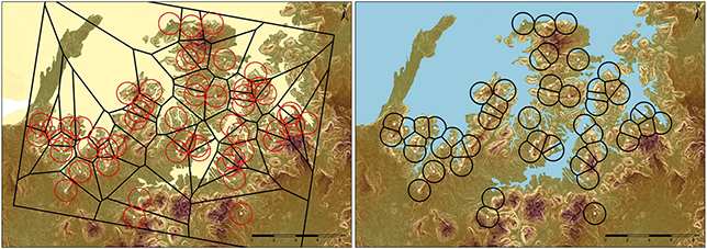
Figure 4 diagram presents a Model Builder workflow that is specifically designed to generate concentric buffer rings around a set of initial points while systematically analyzing the spatial characteristics of the surrounding environment. This workflow automates the process of extracting, processing, and quantifying spatial data within a defined polygonal area. It is structured to handle various stages of spatial analysis, encompassing data input, feature selection, buffer creation, spatial extraction, data processing, and aggregation. The first stage of the model involves two primary input layers: One containing the initial points, which represent the sites or features of interest, and another specifying the polygonal area that is to be analyzed. The process begins with the “Iterate Feature Selection” step, which iterates through the point features, processing each one independently.
Workflow of different tools for the buffer model
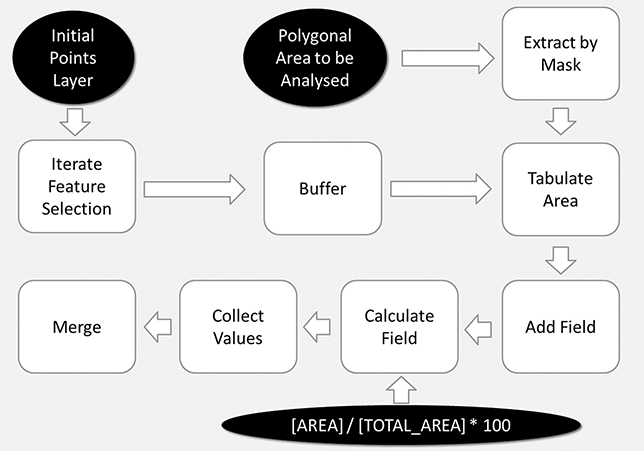
In the next stage, the model generates a buffer around the selected point, creating a zone with a defined distance. This buffer represents a concentric analysis ring, which forms the basis for further spatial analysis. The subsequent step utilizes the “Extract by Mask” tool, which clips the spatial data within the polygonal analysis area, thereby restricting the analysis to the predefined study region. Following this, the “Tabulate Area” function is employed to calculate the area of different categorical spatial elements, such as land cover, soil types, or elevation classes, within the buffer zone. This spatial categorization aids in understanding the distribution of different environmental factors within the region of interest.
Data processing is then carried out by adding a new field to store the calculated values, which is done using the “Add Field” step. The “Calculate Field” tool is then applied to compute a percentage value that normalizes the extracted area relative to the total area. This is achieved by using the formula:
(AREATOTAL_AREA) × 100\left(\frac{AREA}{TOTAL\_AREA} \right) \times 100(TOTAL_AREA\AREA) × 100
This calculation ensures that the proportion of each spatial category within the buffer is standardized in relation to the total analysis area, enabling a consistent and comparable measurement of spatial features.
Finally, the model aggregates the processed data through the “Collect Values” step, which gathers the relevant spatial data for each buffer. The “Merge” function is subsequently applied to combine the individual buffer outputs into a single, consolidated dataset. This final dataset is then ready for further interpretation and visualization, providing a comprehensive view of the spatial relationships and environmental conditions within progressively larger areas surrounding the initial points.
This Model Builder application methodically processes spatial data by constructing concentric buffers around point features, extracting pertinent environmental information from within these zones, and calculating the proportional representation of various spatial factors. The outcome is a structured dataset that enables the interpretation of environmental conditions and spatial relationships across expanding areas surrounding the original points of interest.
3.2.2 Topographic Model
Regarding the study of distances incorporating topography, or equivalently, the calculation of average travel times, two principal approaches emerge. The first approach involves conducting an LCP analysis to derive isochrones that represent coherent travel times in terms of energy expenditure. In the given example, the Tobler algorithm is employed due to its simplicity and practicality, although several other algorithms exist that operate on similar principles. For the mobility component, we implement Tobler’s hiking function, an empirical relationship that converts terrain slope into walking speed and thus into travel time. The function peaks at a slight downhill grade (about −5%) and penalizes both steeper ascent and descent. Applied via raster algebra, this yields time surfaces and isochrones that respect topographic friction rather than distance alone. Because direction matters, outbound and inbound costs can be computed with the forward and inverse forms and then averaged to approximate round-trip times, which is the relevant unit for daily mobility to and from fields.
We choose Tobler because it is the classic and simplest option: Transparent, easy to reproduce, and widely understood, qualities that facilitate comparison across sites and studies. Other functions discussed later in the text (e.g., Llobera and Sluckin, Reference Llobera and Sluckin2007; Baek and Choi, Reference Baek and Choi2017) adjust the slope–speed relationship and can be preferable in particular terrains (e.g., very rugged, high-relief settings) or when one needs stronger uphill/downhill asymmetries. Whether the choice of function materially affects results depends on terrain and conditions. For evaluating how long a person would take to walk to a field, work, and return the same day, Tobler is often a strong choice: Daily agrarian commutes typically involve short to moderate distances on mixed but not extreme gradients; the function captures the dominant constraint (slope) with a realistic downhill advantage and an uphill penalty; averaging forward and return legs provides a pragmatic round-trip estimate; and the model’s simplicity avoids over-tuning to local idiosyncrasies while remaining sensitive to topographic variation.
This methodology generates isochrones that define travel ranges from or to a location, estimating the time needed to reach destinations and, by doubling, approximating round-trip durations. The choice of time threshold depends on context: For example, a 30-minute radius may suit daily mobility better than a one-hour trip. These analyses incorporate topographic constraints but usually calculate only outbound costs; a more realistic solution is to model both outbound and return trips separately and then average the results through raster calculations. While useful where property boundaries are undefined, the method considers only displacement distance, and accuracy could be improved by correlating results with cadastral data.
To refine estimates, an iterative approach can be applied: Computing isochrones from each analysis point, extracting values from a reclassified friction map for a given time threshold, converting cost surfaces into polygons, and compiling tabulated datasets with percentage areas. This provides highly precise reconstructions of mobility rings and agricultural potential, though it is computationally demanding and risks overlap when buffers exceed average point spacing, introducing comparative data from different areas. It is important to stress that this approach does not aim to delineate exact property limits but rather to model functional mobility zones, within which individuals could feasibly access multiple nearby properties.
An alternative, more straightforward method for delineating more clearly defined property areas, as opposed to buffer rings, is the incorporation of a cost allocation tool. This type of analysis is used to define areas of influence based on various distance or cost metrics. In such cases, a model can be created using a friction map combined with an approximate calculation of the areas of influence. Although this approach may be less realistic in terms of absolute distances, since the limit is determined by adjacent properties, it is particularly useful in areas where there is high confidence in the underlying data, whether due to well-understood geological deposits or reliable cadastral records. The outcome of the analysis will vary depending on the base map employed. For example, the analysis can be executed directly using terrain slopes in a path distance allocation, yielding influence areas for each point relative to others, thereby offering a topographically realistic perspective.
Alternatively, a cost allocation analysis utilizing a mobility algorithm similar to the Tobler (Reference Tobler1993) approach can be performed, which produces markedly different results and provides insights into the influence of each method. It is important to be cautious when performing cost allocation, as the results can vary significantly depending on whether a standard friction map is used or if an algorithm is incorporated into the process. The following image illustrates this substantial difference: On the left, a standard cost raster is shown (where slopes are simply constrained by rivers and coastlines), whereas on the right, the same raster incorporates Tobler’s algorithm. It is always recommended to employ analyses that take this variance into account, even if the specific algorithm is not used, in order to achieve a more realistic representation of the landscape (Figure 5).
Cost allocation with standard friction map in left and the same analysis but using a Tobler function in right. A larger version of this figure is available to view at www.cambridge.org/spatial-analysis
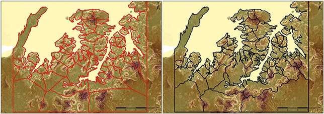
The most coherent strategy, however, is to combine both approaches. This entails integrating a travel cost analysis with a cost allocation analysis to achieve boundaries that respect topographical constraints while simultaneously considering travel time. As discussed, the travel cost analysis can be refined by employing an algorithm such as Tobler’s, which estimates the walking time required to reach a destination. Mobility rings can be classified using a threshold, for example, 0.25, which corresponds to 15 minutes. Consequently, a round trip would require 30 minutes, a duration that is deemed reasonable for various activities. In cases where properties are closely spaced, and a 15-minute threshold may encompass several centers, the method can be refined by incorporating cost allocation to precisely delineate the area. The simplest procedure involves calculating both cost surfaces, converting them to polygons (with the travel cost layer pre-classified to the desired value, such as 0.25), and finally using an intersect tool to derive the overlapping area between the two polygon sets. This overlapping area, as in Figure 6, is then analyzed to determine the respective areas of influence. It is important to note that during these transformations, two grid codes are produced: One corresponding to the travel cost, which may not be directly meaningful, and another corresponding to the cost allocation, which accurately identifies the central point of origin. It is critical to select the appropriate field of reference to ensure the statistical analyses are conducted correctly.
Isochrones made by path analysis in left and cropped areas with a 15 minutes walking in right using combination of cost allocation and path distance.
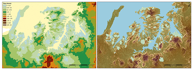
Figure 7 diagram illustrates a Model Builder workflow designed to analyze the path distance from a set of origin points, using a friction raster to compute the distance calculations, and subsequently generating influence areas in time based on spatial analysis. Unlike the previous model, which focused on creating concentric buffers, this workflow begins with the calculation of path distances, utilizing a friction raster to determine the resistance or difficulty of movement through various terrain types. The process begins with the input of two primary layers: A raster of friction and the origin points layer, which represents the starting locations for the analysis.
Workflow of cost distance model.
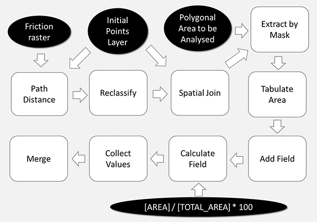
In the first step of the model, the path distance is calculated using the friction raster and the origin points. The friction raster provides the necessary data on movement resistance, while the origin points serve as the starting locations for the path distance calculations. This process determines the travel cost from each point, creating a path distance raster that represents the minimum cost to travel from each cell to the nearest origin point, factoring in the friction values of the raster. The resulting path distance raster is then reclassified to generate an area of influence, where each pixel represents the distance (or time) required to reach the origin point, considering the terrain’s characteristics. To further refine the analysis, algorithms such as Tobler’s Hiking Function (Tobler, Reference Tobler1993), which is commonly used for modeling movement in terrain, can be applied to adjust the path distance values, transforming them into an influence area in terms of time rather than just distance. This allows for a more nuanced understanding of how terrain affects movement over time, and it helps to model real-world conditions more accurately. We could use, for instance, other formulas, like LLobera and Sluckin function (Reference Llobera and Sluckin2007), more accurate for mountainous landscapes, or others like Baek and Choi (Reference Baek and Choi2017).
Once the area of influence is defined, the next step in the process uses the “Spatial Join” tool to combine the resulting polygons, effectively uniting the individual areas of influence into a single polygonal region for further analysis. This spatial join step is crucial because it aggregates the distinct influence zones into a unified area that can then be analyzed in greater detail. Unlike the buffer-based model, where the buffer distance remains the same for each point, the path distance-based approach results in polygons of varying sizes and shapes, as the influence area will differ for each point depending on the terrain and the friction raster values. After the spatial join, the model proceeds with the same procedures as in the previous workflow.
3.3 Method to Compare Multiple Layers
At this point, I describe the methodology for implementing the analysis, whether it is buffer-based or topographic, using multiple parameters simultaneously. In the previous examples, the fundamental task was to extract spatial information around a specific location, relying on a single dataset as the reference. However, the method proposed here differs by combining multiple different parameters into a single dataset. To make this approach comparable, it is necessary to classify the information based on the specific requirements and the number of parameters involved, as outlined in the following. For practical purposes, I will directly illustrate the classification of soils, which will be developed in the following examples. Specifically, this will focus on soil types, terrain orientation, and slopes.
The soil classification data presented is based on the system described in Trapero (Reference Trapero Fernández2024) by Bloomsbury. Each record is identified by a unique ID and corresponding UNID_EDAF designation, with a numerical classification value and a justification for that classification (Table 4). For example, ID 0 corresponds to Arenosols (Arenosoles álbicos), Humic Cambisols (Cambisoles húmicos), and Dystric Gleysols (Gleysoles dístricos), which are assigned a value of 300. Although Arenosols are generally poor, the presence of Cambisols and Gleysols can enhance soil fertility. In contrast, ID 1, comprising Calcareous Cambisols and Calcic Regosols associated with Litosols, Calcareous Fluvisols, and Vertic Cambisols, is assigned a value of 400, reflecting soils that are generally good for agriculture yet may present drainage issues. Other entries detail soils with saline characteristics (e.g., ID 2: Takiric and Gleyic Solonchaks with a classification of 200) and soils of variable fertility and structural quality, such as those with moderate fertility but potential depth limitations (ID 3) or fertile soils prone to waterlogging (ID 4). The classifications continue in a similar manner, with values ranging from 100 for very poor, stony soils (ID 20) to 500 for deep and fertile soils ideal for intensive agriculture (e.g., IDs 11, 13, 14, 15, and 21).
| ID | UNID_EDAF | Value | Justification |
|---|---|---|---|
| 0 | Albic Arenosols, Humic Cambisols, and Dystric Gleysols | 300 | Arenosols are poor, but Cambisols and Gleysols can improve fertility. |
| 1 | Calcareous Cambisols and Calcareous Regosols with Litosols, Calcareous Fluvisols, and Vertic Cambisols | 400 | Good agricultural soils, but they may have drainage issues. |
| 2 | Takiric Solonchaks and Gleyic Solonchaks | 200 | Saline soils, limited for agriculture. |
| 3 | Calcareous Regosols and Calcareous Cambisols with Litosols, Calcareous Fluvisols, and Rendzinas | 400 | Moderately fertile soils, with some depth limitations. |
| 4 | Pelic Vertisols and Chromic Vertisols | 400 | Fertile but prone to waterlogging in winter. |
| 5 | Dystric Regosols and Arenosols (Dunes and Beaches) | 300 | Sandy soils, poor for intensive agriculture. |
| 6 | Chromic Vertisols and Vertic Cambisols with Calcareous Cambisols, Calcareous Regosols, and Pelic Vertisols | 400 | Medium-high fertility, but at risk of waterlogging. |
| 7 | Litosols, Chromic Luvisols, and Rendzinas with Calcareous Cambisols | 300 | Litosols limit their use, but Cambisols and Luvisols improve quality. |
| 8 | Eutric Cambisols, Chromic Luvisols, and Litosols with Dystric Cambisols and Rankers | 300 | Medium fertility, but the presence of Litosols and Rankers reduces productivity. |
| 9 | No data | – | – |
| 10 | Eutric Planosols, Gleyic Luvisols, and Plinthic Luvisols | 400 | Good soils, but may have drainage issues. |
| 11 | Calcareous Fluvisols | 500 | Fertile soils in alluvial plains, ideal for intensive agriculture. |
| ID | UNID_EDAF | Value | Justification |
|---|---|---|---|
| 12 | Eutric Regosols, Dystric Regosols, and Albic Arenosols | 300 | Poorly developed soils, with limited fertility. |
| 13 | Eutric Fluvisols and Eutric Cambisols | 500 | Highly fertile, optimal for wheat and similar crops. |
| 14 | Calcareous Luvisols, Calcareous Cambisols, and Chromic Luvisols with Calcareous Regosols | 500 | Well-structured and fertile soils. |
| 15 | Calcareous Cambisols, Calcareous Luvisols, and Chromic Luvisols with Litosols and Calcareous Fluvisols | 500 | Deep and fertile soils, ideal for rainfed crops. |
| 16 | Pelic Vertisols, Rendzinas, and Calcareous Regosols | 400 | Fertile soils, but prone to waterlogging. |
| 17 | Mollic Planosols, Pelic Vertisols, Calcareous Phaeozems with Sandy Rankers | 300 | Soils with drainage limitations and sandy texture. |
| 18 | Vertic Cambisols, Chromic Vertisols, and Calcareous Cambisols with Calcareous Regosols | 400 | Medium fertility, but at risk of waterlogging. |
| 19 | Calcareous Cambisols, Calcareous Regosols, and Litosols with Rendzinas | 300 | Soils with limitations due to the presence of Litosols. |
| 20 | Eutric Regosols, Haplic Xerosols, and Litosols | 100 | Very poor and rocky soils. |
| 21 | Calcareous Luvisols, Chromic Luvisols, and Gleyic Luvisols | 500 | Deep and fertile soils. |
| 22 | Vertic Cambisols, Calcareous Regosols, and Chromic Vertisols with Calcareous Cambisols | 400 | Medium fertility, but at risk of waterlogging. |
| 23 | Chromic Luvisols, Calcareous Cambisols, and Litosols | 400 | Fertile, but the presence of Litosols reduces productivity. |
| ID | UNID_EDAF | Value | Justification |
|---|---|---|---|
| 24 | Chromic Luvisols and Regosols | 400 | Fertile but poorly developed soils. |
| 25 | Chromic Luvisols, Eutric Cambisols, and Litosols | 400 | Fertile soils, but with the presence of Litosols. |
| 26 | Eutric Cambisols, Rankers, and Orthic Luvisols | 300 | Soils with medium fertility, but the presence of Rankers limits their agricultural use. |
In addition to the soil classification, the study delineates three primary thresholds based on terrain slope, derived from a weighted mean of overall slopes in the territory. The first threshold identifies low-lying, nearly flat zones that are considered optimal for extensive cereal cultivation. The second threshold comprises areas with moderate slopes, typically between 5° and 10°, which correspond to small hills or inclined zones; slopes of less than 5° are treated as relatively flat. The computed weighted mean slope for the area is approximately 5°, providing an indication of the general steepness of the terrain.
The slope analysis is fundamentally important, not only for understanding the physical characteristics of the terrain but also for evaluating the impact of shading and wind protection. Historical evidence suggests that during the Roman era, strong easterly and southerly winds were prevalent in the region. Contemporary observations indicate that eastern winds remain frequent, with gusts exceeding 50 km/h for extended periods, a phenomenon that poses a risk during critical phenological phases such as flowering. Similarly, the summer season is characterized by the strong winds originating from Africa, which persist over long durations and can adversely affect plant health (Columella, Rust. 3.12.6).
These meteorological and topographical considerations necessitate a careful analysis of aspect, as the orientation of the land directly influences both insolation and wind exposure. Although a southern orientation is generally preferred to maximize insolation and avoid the shading effects associated with northern exposures, the prevalent wind conditions may preclude such an orientation. In this context, an orientation toward the west may be optimal. Consequently, the study proposes a classification of aspects into four major groups, each with relevant subcategories based on orientation:
1. Group One: Areas with an orientation that is favorable for both wind conditions and solar insolation, primarily in the west and southwest.
2. Group Two: Areas that are well-situated with respect to wind but less optimal in terms of insolation, typically corresponding to the northwest and north.
3. Group Three: Areas that receive favorable solar insolation but are more vulnerable to adverse wind conditions, generally found in the south and southeast.
4. Group Four: Areas considered less favorable for both wind exposure and insolation, usually oriented toward the east and northeast.
This classification provides a framework for understanding the interaction between topography, soil properties, and climatic influences, thereby enabling more informed decisions in land management and agricultural planning. By integrating these factors, GIS-based analyses can better predict areas of high productivity and areas where additional management interventions may be necessary to mitigate the impacts of adverse terrain and meteorological conditions. Based on these criteria, we can clearly define the areas to be studied. Essentially, this involves integrating the three selected criteria into a single raster. The reclassification process follows the methodology outlined in the annexed tables, which serve as a reference for data processing.
A simple technique is used to achieve this classification: Each raster value is multiplied by units, tens, and hundreds. This means that a classification value of 111, for example, would represent poor-quality soil, oriented toward the sun, and situated on flat terrain. Once the values are extracted, they can be reclassified into more comprehensible and practical categories, as shown in Tables 5 and 6:
| Slope (P) | Wind (V) | Comment and Group |
|---|---|---|
| 1 (flat) | 40 | Group 1: Ideal for cereal cultivation (flat land with excellent orientation). |
| 1 (flat) | 30 | Group 1: Although V = 30 indicates slightly reduced orientation, the high soil quality and flatness make it viable for cereals. |
| 1 (flat) | 20 | Group 2: Poor orientation for agriculture but benefits from high-quality soil. |
| 1 (flat) | 10 | Group 3: Despite optimal soil, very unfavorable orientation (strong winds/poor solar exposure) downgrades it to livestock use. |
| 2 (moderate slope) | 40 | Group 2: Excellent for vineyards/olive groves (optimal soil, moderate slope, and perfect orientation). |
| 2 (moderate slope) | 30 | Group 2 |
| 2 (moderate slope) | 20 | Group 3 |
| 2 (moderate slope) | 10 | Group 3: Moderate slope combined with poor orientation makes it less suitable; livestock use is recommended. |
| 3 (steep slope) | Any V | Group 3: Even with optimal soil, steep slopes hinder mechanization, making it more suitable for livestock. |
| Slope (P) | Wind (V) | Comment and group |
|---|---|---|
| 1 (flat) | 40 | Group 1: Suitable for cultivation, but only if the orientation is excellent. |
| 1 (flat) | 30 | Group 1: Good soil with reduced orientation is downgraded; livestock is suggested. |
| 1 (flat) | 20 | Group 2 |
| 1 (flat) | 10 | Group 3 |
| 2 (moderate) | 40 | Group 2: Favorable for vineyards/olive groves but requires optimal orientation; otherwise, it is assigned to livestock. |
| 2 (moderate) | 30 | Group 2 |
| 2 (moderate) | 20 | Group 3 |
| 2 (moderate) | 10 | Group 3 |
| 3 (steep) | Any V | Group 3: Steep slopes make intensive farming less viable. |
For cultivable but poor soil (S = 300): All combinations (with any P and V) result in values ranging from 311 to 343 and are classified as Group 3 (suitable for extensive livestock farming) due to low fertility, which limits their use for intensive crops.
For saline soil (S = 200): Regardless of slope and wind conditions, values 211 to 243 are assigned to Group 3 – these soils are typically used for livestock farming.
For very poor/rocky soil (S = 100): Any combination (values ranging from 111 to 143) is assigned to Group 4, meaning these lands are unsuitable for cultivation or livestock. Instead, they may be designated for forestry, conservation, or other nonagricultural uses.
As can be seen in this data classification, the number of elements integrated is scalable, depending on the parameters we wish to include. It also allows for the establishment of ranges with up to nine or ten different values for each assignment, which implies that no further numerical classifications can be considered beyond this. In any case, this is a straightforward approach to address this issue and establish common ranges for a unified analysis, such as the zones defined based on land use. In the following sections, the results of this classification will be applied in various models and compared with each other.
3.4 Assumptions, Limitations, and Analytical Potential
This section is dedicated to addressing the potential methodological limitations of the RBASE model and proposing strategies to mitigate them. Two key aspects are considered. First, the definition of the mobility range or buffer zone used in the analysis is critical, as variations in its extent significantly affect the resulting values and spatial interpretations. Second, attention is given to the comparative analysis of these concentric zones, as their statistical examination becomes a data source in its own right. By conducting multi-scalar analyses, it becomes possible to generate diverse datasets that can be systematically compared, thereby offering a valuable tool for understanding spatial behavior and settlement dynamics at varying levels of resolution.
The selection of appropriate buffer radii is a methodologically critical decision, as it fundamentally dictates the spatial scales at which site-catchment relationships are initially interrogated. Arbitrary distances risk analytical detachment from historical realities. The criteria can be different, depending on the scope. We can deliberately calibrate using historically relevant proxies derived from Roman agrarian practices and land management principles (Carandini, Reference Carandini1994; Witcher, Reference Witcher2006). Primary reference was made to the characteristic dimensions associated with Roman centuriation (land division) systems and the standard units of land measurement, such as the actus (approx. 35.5 m). The centuria itself, a widespread module in Roman agricultural landscapes, typically presented dimensions approximating 20 × 20 actus (roughly 710 × 710 m), although variations existed. Deriving plausible radii from such units (e.g., considering the radius of a circle inscribed within a half-centuria, ~283 m, or related fractions/multiples) provides a nonarbitrary, historically grounded basis for establishing analytical zones directly relevant to the likely scale of Roman agricultural exploitation, property demarcation, and routine short-range mobility within the immediate farmstead environment.
However, this is a complex problem to analyze, and even more so to define precisely, considering that the ranges are different and their utility is highly intricate. In this Element, I have dedicated a section to understanding which mobility ranges are ideal for their application, as well as the significant differences between them. This also represents an improvement in the information obtained, as calculating different mobility ranges and comparing them allows us to understand how an archaeological site relates to its immediate surroundings or more distant areas.
These analyses have been carried out using several ranges of 100, 200, 500, and 1,000 m. In addition, the range corresponding to a Roman century of 283 m has also been considered, which had already been published in a previous work (Trapero, Reference Trapero Fernández2021b). In this case, the ranges finally applied were selected on the basis of specific logical criteria rather than probabilistic ones. The first criterion was the use of different ranges, since in the various tests performed it became evident that the results displayed a certain degree of similarity depending on the ranges employed. In other words, short buffer ranges tend to resemble each other considerably, even when compared with short ranges of distance-cost times. This similarity is primarily due to issues related to data quality. For example, in fields such as geology or soil studies, the resolution is not sufficiently precise, and the available data are not entirely accurate but rather generalized, which reduces their reliability at very small scales. A similar problem arises with larger ranges, where the main issue lies in the overlap and mixing of one area with another.
The methodology generates isochrones to estimate travel times from or to a location, doubling values to approximate round trips, with thresholds adapted to context (e.g., 30 minutes for daily mobility). While it accounts for topographic constraints, it often models only outbound costs; more realistic results come from averaging separate outbound and return analyses. Accuracy can improve by correlating results with cadastral data, though where boundaries are absent, an iterative approach is applied: Computing isochrones from each point, reclassifying friction maps, converting cost surfaces into polygons, and tabulating percentage areas. This yields precise reconstructions of mobility rings and agricultural potential, though computationally demanding and prone to overlap if buffers extend beyond average spacing. Rather than defining property limits, the method models functional mobility zones, recognizing that individuals could access multiple nearby properties.
As has been observed, the determination of areas of influence relies on the calculation of an average between sites, so that soils, slopes, or any other variables the researcher wishes to include are not erroneously recorded. A second criterion was the selection of two specific distance ranges, 100 and 1,000 m, since it is preferable to carry out two complementary analyses instead of a single one. One of these serves to understand the immediate surroundings of the villa, while the other provides insight into the more distant context. These are compared, in this particular case, with the 15-minute cost-distance range, which represents an intermediate scale that is considered to reflect reality more effectively. Other ranges, such as 60 minutes or 10 minutes, could also have been compared along with the rest. However, it was deemed unnecessarily complex to introduce so many different comparative scenarios.
It must therefore be emphasized that no single range is intrinsically superior to another; the appropriateness of a range depends entirely on the specific historical question posed by the researcher. The comparative analysis between 100 m, 1,000 m, and 15 minutes is designed to ensure that any user wishing to reproduce the study is capable of choosing one range or another, understanding not so much the absolute value of “100 m” itself, but rather the meaning behind the number. That is to say, when analyzing multiple sites, the difference between 90, 100, or 110 m will not be statistically significant, whereas the distinction between analyses at 100 m or at 1,000 m becomes highly relevant.
In order to determine which spatial scale (distance-based buffers (100 m, 1,000 m) or a travel-time-based buffer (15-minute ring)) is better for different historical questions, a systematic comparative analysis is required. This evaluation involves applying a series of statistical and spatial analyses to assess how soil type distributions vary across different buffer zones and to identify which scale provides the most relevant insights.
The first step is to conduct a direct comparison of soil type percentages at each site across the three buffer zones. By examining whether the proportion of each soil type remains stable, increases, or decreases as the buffer expands, I can assess the degree to which each scale captures meaningful spatial patterns. For example, if a particular soil type constitutes 40% of the area within a 100-m buffer, I analyze whether this percentage remains similar in the 1,000-m buffer or shifts significantly in the 15-minute travel ring. Calculating the average percentage difference between buffers allows us to quantify these changes and determine whether certain buffer sizes are more sensitive to soil variations.
The analysis of each data across different buffers and travel-time rings involves calculating statistics to evaluate variability, detect trends, and identify anomalies that influence interpretations of spatial scale. By comparing values such as mean, median, standard deviation, and range across 100-m, 1,000-m, and 15-minute rings, it becomes possible to assess whether soil types are evenly distributed or concentrated at specific scales. Observing systematic increases or decreases in soil percentages with distance highlights localized versus widespread features, while detecting outliers, such as unusually high concentrations at certain sites, helps refine interpretations of geomorphological influences. Finally, examining changes in variability across scales indicates whether soil distributions become more homogeneous at broader extents or remain heterogeneous due to localized conditions, thereby clarifying whether distance-based or time-based methods better capture relevant spatial patterns. Here are some statistics that can be calculated depending on the base data (e.g., orientation is 360º data is different as class type of soils):
Mean
Median
Standard deviation
Range
Percentage change across scales
Trend analysis (increase/decrease with distance or time)
Outlier detection (comparison with overall averages)
Homogeneity/heterogeneity assessment (changes in variability with scale)
By combining fixed-distance (100 m, 1,000 m) and travel-time (15 minutes) analyses, the model does not seek a universal standard but instead highlights how each spatial scale generates distinct datasets that reveal different aspects of ancient spatial behavior. Proximate zones are generally associated with stronger site influence, daily activities, and localized land use, while more distant areas tend to reflect broader regional dynamics. This multi-scalar perspective underscores the importance of mobility in resource acquisition strategies and shows that different scales correspond to varied economic, social, and functional relationships with the landscape, making their integration essential for archaeological spatial analysis.
4 Model Application to Hasta Regia and Results
A dedicated section presents the results of the method applied to a practical case study of my choice, based on both the reliability of the available data and their effective integration (Trapero, Reference Trapero Fernández2021a). For each case, the results are evaluated not only in general terms but also with respect to the differences that arise from the use of various distances and analytical approaches. The objective is not to provide specific historical data, since this constitutes a theoretical application using datasets whose reliability allows me to demonstrate the implications of applying one range or another to potential outcomes. For this reason, this section combines the application of the method across three different ranges. This does not imply that an interested researcher must necessarily perform these three analyses; rather, it is intended to illustrate the errors and advantages that each range and method (buffer analysis or cost-distance analysis) may present depending on the historical question posed. Consequently, the discussion is of a more interpretative nature, though it is grounded in the use of real data.
The following image illustrates these parameters for the study area, using the criteria applied in the previous sections:
To facilitate the comparison of results obtained from the three models applied at distances of 100 m, 1,000 m, and a 15-minute travel time, a series of stacked bar charts is presented in Figure 8. These charts quantitatively summarize all computed values, enabling the reader to assess the outcomes across the different spatial scales and to establish meaningful correlations between data points. It is important to note that the legend indicating the number of sites represented is provided in Table 1, located in Section 1.1, which outlines the contextual background of the case study.
Slope gradient in degrees up left, orientation of the terrain up right, and soils classification down.
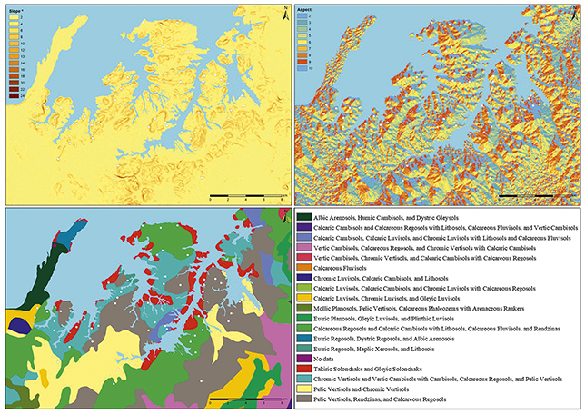
4.1 Slope
As can be seen in the previous Figures 9, 10, and 11, the results are quite different. The first parameter under consideration is the terrain’s slope, which I quantify as the gradient in degrees relative to a vertical plane (90°). For each location, I record two values within the [0°, 90°] interval, although most slopes cluster around moderate inclines due to the inherent topography of the study area. I compare three distinct analytical scales, buffers of 100 m, 1,000 m, and a 15-minute topographic mobility radius, and observe substantial variation among them.
Analysis of slope gradient with a buffer ring of 100 m
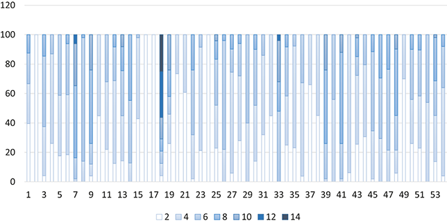
Analysis of slope gradient with a buffer ring of 1,000 m
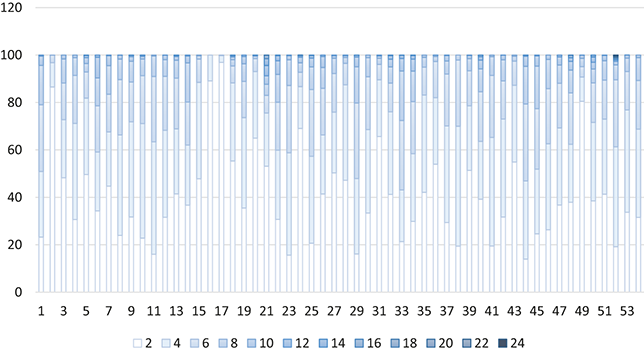
Analysis of slope gradient with an isochrone of 15 minutes
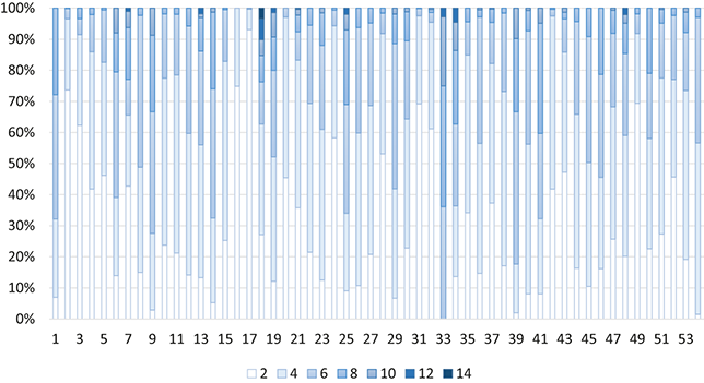
At the 100 m scale, representing a much localized context, only a small fraction of the ground exhibits gradients exceeding 7°, and gradients above 29° are exceedingly rare. In fact, approximately 80% of the area in these 100 m buffers lies above 7° of slope, indicating that steep inclines dominate the immediate surroundings of the surveyed villas. Conversely, the broader buffers (1,000 m) display an average incline closer to 2%, with just 44% of their area surpassing this low threshold. This inversion of slope distribution between scales reveals that, while individual villas sit atop relatively steep hills, the surrounding landscape at larger extents is comparatively gentler.
Such a pattern is coherent with the spatial organization of these settlements: The villas themselves are typically situated on mid-slope positions, elevated enough to provide strategic vantage points but not on the steepest escarpments, whereas adjacent terrain flattens into more manageable agricultural plots. Bearing in mind that a hectare (10,000 m²) is often regarded as the minimum unit for viable cultivation, the predominance of moderate slopes in the wider buffers implies sufficient area for farming activities, despite the immediate vicinity of each villa being rugged.
Turning to measures of central tendency and dispersion, both the mean and median slope values increase with buffer size, whereas variability, expressed as standard deviation, decreases. Steeper slopes (6°–10°) thus diminish in proportion as one moves from the 100 m to the 1,000 m scale: Areas above 10° drop from 6.2% at 100 m to just 2.1% at 1,000 m.
The 15-minute mobility radius, which incorporates the effort required to traverse the landscape, further accentuates these differences. Within this temporal buffer, certain points exhibit extreme gradients that would significantly alter travel dynamics; heterogeneity here is captured by higher standard deviations compared to more homogeneous slope fields. Yet even at this intermediate scale, the overall consistency of slope values across most locations remains evident, reinforcing the idea that larger observational extents smooth out local idiosyncrasies.
Collectively, the visual and statistical analyses underscore a clear settlement pattern: The villa occupy positions of moderate incline, whereas their broader environs are characteristically flatter. This configuration likely reflects a balance between defensive or visibility advantages afforded by elevation and the pragmatic demands of agriculture and transport. Moreover, the scale-dependent behavior of slope distributions suggests that very small buffers (100 m) are insufficient to capture the full spatial context of each villa, whereas extremely large extents (on the order of 1 km or more) may obscure locally significant terrain features. Consequently, intermediate ranges, such as the hectare-scale or the 15-minute mobility zone, appear most informative for understanding both the functional and locational aspects of these settlements.
In fact, slope proves to be a qualitatively valuable metric for assessing territorial variance and identifying potential settlement patterns. While the majority of the study area resides on lower inclines, mean slopes intensify in the immediate vicinity of occupation sites, indicating deliberate placement on mid-slope terrain rather than on flat plains or steep ridges. This insight will guide further modeling efforts aimed at elucidating the interplay between topography, land use, and settlement distribution.
The analysis of slope in the territory of Hasta Regia proves to be highly valuable for understanding settlement patterns, particularly in relation to the location of villas. It becomes evident that the majority of these establishments were positioned in areas that can be considered favorable for their development and sustainability. This observation is consistent with what has previously been demonstrated in connection with the relationship between villas and agronomic precepts (Trapero, Reference Trapero Fernández2021a).
From a critical perspective, the usefulness of slope analysis does not merely lie in confirming that villas occupy advantageous terrain; rather, it highlights the deliberate choices made in the siting of these complexes. The preference for areas with manageable gradients reflects an understanding of both agricultural potential and practical accessibility, reinforcing the idea that these decisions were guided by coherent, pragmatic criteria rather than by chance. At the same time, the finding invites further discussion on the degree to which agronomic prescriptions shaped settlement strategies, raising the question of whether the villas conformed strictly to theoretical models or whether local conditions prompted nuanced adaptations. In this sense, slope functions not only as a geographical parameter but also as an interpretative lens through which social, economic, and cultural dimensions of Roman rural organization can be reconsidered.
4.2 Aspect
The second parameter I examine is terrain aspect, categorized into eight directional sectors: North, north-east, east, south-east, south, south-west, west, and north-west, each quantified as the percentage of surface area falling within that sector. When I juxtapose the three analytical scopes (100 m buffer, 1,000 m buffer, and 15-minute mobility radius in Figures 12, 13, and 14), no unambiguous bias toward any single aspect emerges, in contrast to the clear patterns observed for slope. This absence of a dominant orientation is not surprising: a hilltop typically presents exposures in all compass directions, and a villa perched on such relief must contend with facets on every side. Only where a particular flank of the hill is markedly more gradual or more precipitous would I expect an overrepresentation or underrepresentation of that orientation in the aspect histogram.
Cardinal points orientation of the land in 100 m buffer.
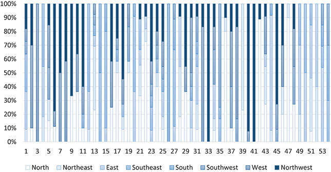
Cardinal points orientation of the land in 1,000 m buffer.
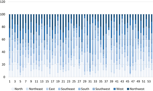
Cardinal points orientation of the land in 15 minutes isochrone.
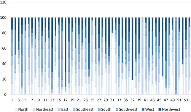
Quantitatively, the percentage of area corresponding to each aspect changes with buffer size. For instance, the easterly sector exhibits higher coverage at the 100 m scale than at broader extents, whereas northerly and north-easterly exposures increase in prominence as the buffer expands. Such shifts reflect the fact that, while immediate vicinities may feature gentle slopes on certain faces, the aggregated landscape at larger scales incorporates additional hillocks and valleys, altering the aspect distribution. Curiously, Site 5 illustrates this phenomenon vividly: Within its 100 m radius, southerly exposures are nearly absent, yet when the buffer is extended, southerly facets account for almost half of the sampled surface. This idiosyncrasy testifies to local topographic complexity.
Across all buffers, the range of aspect percentages typically fluctuates by around 15% indicating moderate sensitivity to analytical scale but without overturning the general pattern of multidirectional exposures. Statistically, I observe that north and north-east aspects tend to gain ground with increasing buffer radius, whereas east and south-west aspects decrease slightly; other sectors remain relatively stable. From a practical perspective, the local (100 m) buffers feature a marginally higher proportion of north-western and north-eastern exposures, a noteworthy point given that prevailing winds in the study region blow predominantly from the south and east. The minimal representation of the south-east sector across most analyses (except the smallest buffer) further underscores the villas’ avoidance of leeward slopes that would be more exposed to desiccating gusts and thus less favorable for habitation and cultivation.
Taken together, these observations imply that very local analyses (100 m) may misrepresent the broader aspect context of a villa, while excessively large buffers obscure fine-grained exposure patterns that could influence microclimatic or defensive considerations. The 1,000 m buffer and the 15-minute mobility radius thus strike a balance: They encompass enough landscape heterogeneity to reveal meaningful aspect distributions without diluting the villa’s immediate topographic setting. In this way, aspect analysis complements slope analysis by demonstrating that, although no single orientation dominates, the villas systematically avoid the most exposed sectors (notably south-east) and instead occupy sites where multiple facets afford a compromise between shelter from winds and access to sunlight. I have in the next paragraph a translation of this Columella reference that helps us to understand the distribution of winds. This data, which in total terms is not noticeable, but in the numerical correlation of the statistics is very significant to understand a pattern that in this case we already knew. This shows at the level of result that the Roman mentality in the distribution of its properties fits with the special logic of the territory, as has already been proposed in previous studies in relation to viticulture in this and other regions (Trapero, Reference Trapero Fernández2016; Stubert et al., Reference Stubert, Oliveras, Märker, Schernthanner and Vogel2020).
Democritus and Mago both extol the excellence of north-facing fields, as they believe that vines oriented in this direction will become highly productive, even if this orientation results in wine of slightly lesser quality. In our view, however, it is preferable to recommend, as a general rule, that in cold regions the vines should face south, and in milder climates, east, provided they are not harmed by the Auster (southern wind) and the Eurus (southeastern wind), as is the case along the coasts of Baetica. If these regions are indeed affected by such winds, it is more advisable to orient the vineyards towards the Aquilo (north wind) and the Favonius
4.3 Soils
The third parameter concerns soil typology, which I classify across three analytical extents as before, yielding markedly different portraits of substrate diversity. At the smallest scale, 100 m (Figure 15), each villa typically overlies a single dominant soil type; for instance, Site 7’s immediate environs are composed almost exclusively of Pelic Vertisol. However, when the buffer expands to 1,000 m (Figure 16), this homogeneity dissolves into a mosaic of additional soil classes. Consequently, the 100 m analysis proves of limited utility for characterizing the broader pedological setting of a settlement. There is no initial difference for 15 minutes isochrones (Figure 17).
Soil analysis using 100 m radius buffer.
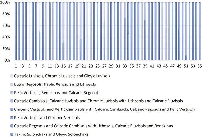
Soil analysis using 1,000 m radius buffer.
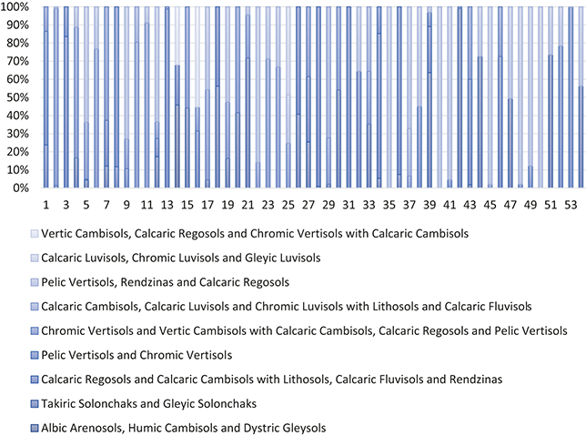
Soil analysis using 15 minutes isochrone.
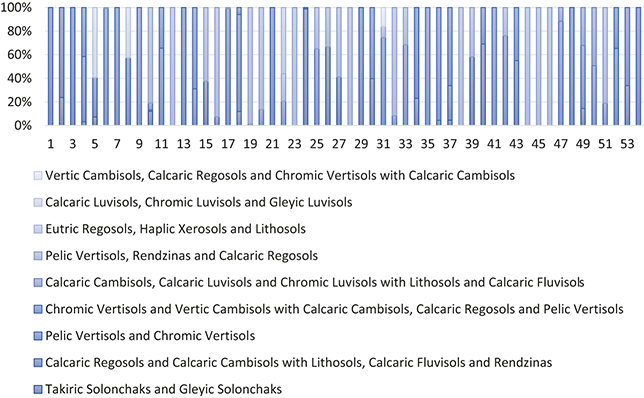
Quantitatively, the proportional variation of each soil class across scales is substantial: Standard deviations on the order of 30% attest to the high heterogeneity induced by buffer expansion. Across the study area, Vertisols emerge as the most ubiquitous group, reflecting both their natural prevalence and perhaps an implicit preference on the part of villa‐site planners. In contrast, calcareous regosols soils appear only in highly localized pockets, likely owing to their fertility and historical association with viniculture, while Solonchaks are distributed more evenly, suggesting less selective placement.
Statistical correlations (Pearson’s R) between soil‐type proportions at small versus large scales are strongest for Vertisols, indicating consistent dominance of this substrate class from the villa’s doorstep out to several hundred meters. Other soil classes, especially those I deliberately omitted beyond the ancient shoreline limit, manifest erratically or are entirely absent, underscoring how our paleo‐coastal cutoff functions as a (human) analytical constraint. Notable outliers occur at Sites 2, 24, and 54, where soil‐type percentages defy regional trends. In Site 24, for example, the apparent overrepresentation of Solonchaks is an artefact of the 15-minute buffer being truncated by topographic barriers, thereby excluding adjacent tracts of arable ground. Such artifacts compel us to question whether certain loci genuinely functioned as self-sustaining agrarian villas or rather as peri-urban estates dependent on external resources.
Broader-scale buffers (1,000 m and 15 minutes) consistently reveal richer soil diversity than the 100 m analysis, yet even these can mask fine‐grained anomalies. At the finest pedometric resolution (c. 25 m grid), calcareous egosols and Cambical Vertisols again dominate, aligning with my observations at the hectare scale. By contrast, intermediate extents (100 m) often present only a singular soil type, occasionally including poorly drained or shallow substrates unsuited to cultivation. Extending the buffer invariably reincorporates these marginal soils, highlighting that small‐scale analyses may inadvertently exclude critical farmland.
Overall, soil‐typology mapping demonstrates that larger analytical extents yield a more representative account of the pedosphere around each villa, while small buffers risk oversimplifying or misrepresenting substrate variability. Crucially, the prevalence of Vertisols and the localized occurrence of calcareous soils suggest deliberate site selection based on agronomic potential, tempered by natural constraints (e.g., paleo-coastal limits and mobility boundaries). Further investigation is needed to disentangle genuine selection preferences from analytical artifacts in those anomalous settlements.
The correlation of soils analyzed in the case study is of considerable relevance when seeking to understand which areas offered the most favorable agricultural conditions. Previous examinations of soil typology have demonstrated a clear relationship in the territory of Hasta Regia between those soils most suitable for vine cultivation and those explicitly referenced by agronomists such as Columella (Trapero, Reference Trapero Fernández2021d). In the present analysis, the results underscore that this relationship is particularly significant in the immediate proximity of the villas.
This outcome is logical if one considers that viticulture required not only specific environmental conditions but also a more specialized labor force, thus exerting a direct influence on the productivity of the estate. The evidence suggests that the economic viability and agricultural success of these rural complexes were closely tied to the immediate landscape, where soil quality played a decisive role. From a critical standpoint, this reinforces the idea that villa placement was neither random nor purely aesthetic, but a deliberate choice shaped by the practical demands of agricultural exploitation. Furthermore, it highlights the extent to which local agronomic knowledge and classical prescriptions overlapped, suggesting that Roman landowners were both responsive to inherited traditions and attentive to the tangible qualities of their immediate environment. Such an interpretation invites further discussion about the balance between theoretical models and pragmatic adaptation in the rural economy of the region.
4.4 Combined Model
The final parameter under scrutiny is land‐use type, categorized into four classes: cereal cultivation, vineyards (and similar crops as olive trees), pastoral activity, and miscellaneous uses, examined at two comparative extents, 1,000 m buffers (Figure 18) and 15 minutes isochrone (Figure 19). I omit the 100 m buffer here, since it merely reflects the footprint of each villa rather than the variability of its broader hinterland, so in this case, it makes no sense to understand something that I already know is broader than the site itself.
Classification of agropastoral areas using 1,000 m buffer.
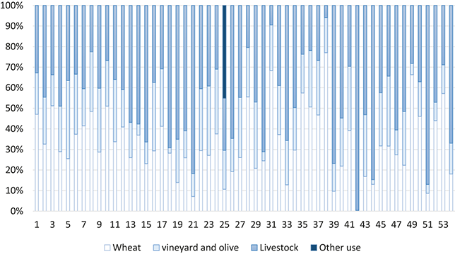
Classification of agropastoral areas using 15 minutes isochrone.
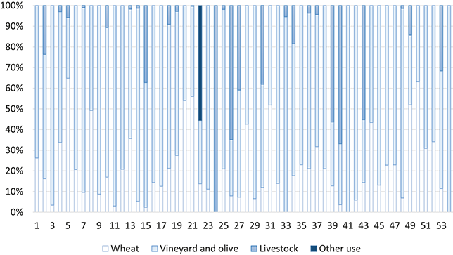
When I compare the 1,000 m against the 15-minute mobility zone, a striking divergence appears in the balance between cereals and vineyards. Specifically, the proportion of cereal lands falls by approximately 15.2% from the 1,000 m buffer to the 15-minute zone, whereas vineyard cover rises by about 21.8% over the same transition. At first glance, one might expect that removing steep slopes (by shifting from a buffer to a topographically sensitive model) would exclude marginal hillside plots and thus favor cereals on gentler terrain; however, the data reveal that vineyards actually become more prevalent when slope constraints are imposed.
Qualitatively, cereals exhibit the most homogeneous distribution across the landscape, whereas vineyards form tightly localized clusters that respond sensitively to topographic constraints. Pastoral areas appear erratic and dispersed, often occupying marginal niches unsuitable for arable production. At larger scales, a correlation between cereal fields and grazing emerges, reflecting a typical Roman biennial cycle: After grain harvest, fields lay fallow and accommodated livestock. Such interleaving of uses underscores the multifunctional character of rural estates.
Finally, the predominance of arable and viticultural land, alongside olive groves, though not explicitly classified here, attests to an overwhelmingly agricultural land‐use regime, with mountainous or forested patches appearing only at a few upland outliers. These anomalies warrant closer scrutiny to distinguish genuine settlement‐related uses from analytical artifacts. In terms of methodological insight, the 25 m topographic model most faithfully captures these nuanced patterns by integrating slope and accessibility constraints, whereas purely radial buffers, despite their simplicity, risk misrepresenting both the extent and suitability of different land‐use categories. Such findings highlight that scale selection is not merely a technicality but fundamentally shapes our understanding of ancient rural economies.
5 Where We Go Next?
The implementation of the RBASE model in the analysis of Colonia Hasta Regia has yielded profound insights into the complex interrelations between ancient societies and their landscapes. By integrating spatial analysis with archaeological data, this model allows for a more nuanced exploration of how past human populations interacted with their immediate environment. This section examines the broader implications of these findings, comparing this approach with previous research and evaluating its potential applicability to other archaeological contexts.
5.1 Comparative Examples of Spatial Models
First, I want to analyze and discuss the data from the results. Building upon the previous analysis, a more comprehensive evaluation of the four analytical dimensions, slope, aspect, soil typology, and land-use categories, provides further insight into the interplay between spatial scales and interpretative limits of each metric. A coherent pattern emerges when these dimensions are considered in conjunction. Specifically, the larger spatial buffers (1,000 m and the 15-minute mobility radius) appear to yield more reliable results in relation to a villa’s siting preferences. The use of very local rings, such as the 100 m scale, captures only idiosyncratic microtopography around the structure itself, without accounting for broader environmental influences. This observation underscores the importance of considering terrain gradient at a larger spatial grain. A villa tends to be located on moderately elevated crests or mid-slope positions (Columella, Rust. 3.1.8), a pattern that could be leveraged as a significant variable in predictive settlement models. However, this would only be valid if the gradient is sampled over a helicoidal band encircling the site, such as 100 m, rather than relying on data derived from a single point datum. Could this nuanced approach to sampling gradients improve the predictive accuracy of historical settlement location models? We must apply the model in several case studies.
The analysis of aspect distributions reveals that larger extents, such as 1,000 m and 15-minute mobility radii, are more effective in capturing systematic avoidance of wind-exposed quadrants (e.g., the southeast), while small buffers merely reproduce the multi-exposures typical of hilltops. This contrast raises a critical question: Do microtopographic features like hilltop exposure dominate settlement choices at small scales, while broader environmental concerns, such as wind protection, only emerge when larger extents are considered? If so, then the scale of analysis becomes a determining factor in the visibility of environmental drivers of human behavior.
Soil-type analysis complicates this picture further. The predominance of Vertisols across scales indicates both natural abundance and possible preferential selection for cultivable loams. Yet, the coarse resolution of published pedological maps, typically designed at national or regional scales, undermines interpretive accuracy at the 100 m level, where localized mosaics are easily misrepresented. Larger buffers, however, capture more edaphic diversity, including fertile calcareous regosols associated with viticulture, suggesting that expanding spatial scales may be essential for identifying land-use strategies tied to complex agricultural practices. This raises a further methodological issue: Could incorporating additional variables, such as lithofacies, hydrography, or road networks, refine land-use models and increase predictive precision?
When physical parameters (slope, aspect, soils) are compared with land-use classes (cereal, vineyards, grazing, miscellaneous), the results highlight a critical interpretive nuance. Slope-based constraints and mobility zones do not simply exclude marginal steep parcels; instead, they underscore the prominence of vineyards within accessible areas. This suggests that land-use cannot be reduced to agronomic logic alone, as socio-economic factors, such as the cultural and economic value of viticulture, may have outweighed environmental constraints. Conversely, pastoral areas tend to retreat into peripheral buffers or truncated zones near impassable relief, where raw percentages exaggerate their actual extent. These points to a methodological need for more refined spatial models capable of integrating terrain, mobility, and social priorities, avoiding simplistic assumptions about the relationship between environment and land use.
These comparative analyses underscore several key points: First, scale selection is crucial for detecting settlement patterns, as different scales reveal different aspects of the environment. Second, point-based metrics, such as those based on 100 m or even 1,000 m buffers, risk overlooking the broader environmental context that frames a villa’s viability. Lastly, the reliability of different data layers, such as topographic versus edaphological data, must be factored into any spatial-statistical model. The question then arises: How can we improve the precision of our predictive models by integrating multiple scales and data layers, especially when considering complex land-use decisions? By incorporating additional environmental covariates, such as detailed geological surveys, hydrographic networks, or paleoenvironmental reconstructions, our understanding of how natural resources and terrain factors jointly shaped the siting of rural elite complexes could be significantly enhanced.
In addition to this comparative analysis, it is necessary to take into account that previous studies, as reviewed in the sections dedicated to the state of the question, have not addressed the specific problem that we are attempting to resolve. The proposal of the RBASE model is, therefore, nothing more than a means of constructing a framework that is more coherent and better adapted to a specific historical question. In other words, it provides a way for a researcher to translate their assumptions and interpretative perspectives into a spatial digital environment, in which many of the issues under consideration are not strictly quantitative but instead qualitative and, in some cases, particularly difficult to measure.
The major challenge with these types of models lies precisely in their limited measurability. Nevertheless, examples such as the Von Thünen model, which has already been analyzed, constitute a useful foundation for our work, since they aim, as we do, to incorporate and reflect historical perspectives within a structured analytical framework. This approach, therefore, seeks not to reduce complex questions to overly rigid numerical parameters but to provide a flexible model that acknowledges the qualitative and interpretative dimensions inherent in historical research.
Site Catchment Analysis has long been valued for its ability to capture fine-grained environmental variability, generate testable economic hypotheses, and link on-site with off-site records, making it foundational in studies of subsistence and early agriculture. Yet, its limits have also been acknowledged: Uncertainties in time–distance parameters (e.g., extended ranges via satellite camps or foraging trade-offs), the central-place assumption when many sites were not residential bases, and difficulties in extrapolating modern environments to the past, especially under technological change.
RBASE addresses these issues by explicitly modeling anisotropy through travel-time and effort over friction surfaces, combining cost-distance and cost-allocation outputs to refine influence areas constrained by topography. In the Hasta Regia sample (fifty-four villas), it reveals scale effects by comparing slope distributions in 100 m buffers, 1,000 m buffers, and 15-minute isochrones, showing mid-slope placements surrounded by gentler terrain at broader scales with implications for agriculture and mobility. By integrating slope, aspect, and soils into transparent classification schemes, RBASE infers land-use suitability (e.g., cereals, vineyards/olive groves, pastoral) through a reproducible pipeline across GIS platforms. Its limitations include sensitivity to algorithm choice, outbound/return asymmetries, potential overlap in iterative isochrones, and computational intensity. Nonetheless, by shifting analysis from Euclidean distance to functional accessibility and contrasting isotropic with anisotropic models, RBASE extends the inferential power of classic SCA while maintaining methodological transparency.
5.2 Broader Implications for Archaeological Research
Archaeological research has long sought to understand the complex interplay between human settlements and the physical environment. Early studies primarily relied on macro-scale analyses to detect regional settlement patterns. Traditional spatial models typically examined distance-based measures and simple proximity to resources, often neglecting the finer details of localized interactions between a site and its immediate landscape. The model represents a significant evolution in this field. It integrates a multidimensional approach that considers various environmental parameters and the inherent costs associated with movement across a landscape. In doing so, it provides a more nuanced interpretation of how ancient populations navigated and utilized their surroundings.
The RBASE model’s development stems from the need to address the limitations of earlier approaches, such as those employed by Llobera (Reference Llobera1996) and Fábrega and Parcero (2009). These studies focused predominantly on large-scale, regional patterns, often overlooking the subtle interactions that occur at the local level. In contrast, my model not only emphasizes local dynamics but also incorporates a variety of geographic parameters into a unified analytical framework. This integration is further enhanced by its cost-surface analysis, which considers both physical distance and the energetic or temporal costs of movement, thereby offering a more realistic assessment of ancient land use. I provide a detailed comparative analysis of the RBASE model with several earlier and contemporary spatial analysis methodologies. I explore both the theoretical underpinnings and the practical implications of these models. Moreover, I will present examples from various studies to illustrate how these different approaches have contributed to our understanding of ancient societies and their landscapes (Cassarotto et al., Reference Casarotto, Pelgrom and Stek2017).
As already explained in Section 2, early spatial analysis in archaeology relied on large-scale models that often oversimplified human–environment interactions. The key ideas are:
Site Catchment Analysis (SCA): Assessed settlement viability based on surrounding resources like water, arable land, and raw materials (Clarke, Reference Clarke1977).
Thiessen Polygons (Voronoi diagrams): Divided landscapes into zones of influence but assumed homogeneity and purely geometric distance.
Gravity Models: Estimated settlement interactions using size and distance but overlooked environmental variability.
GIS-based Approaches: Especially cost-distance analysis, introduced environmental data integration but often retained assumptions of linearity and uniformity (Herzog, Reference Herzog2014).
At the heart of the model developed in this element is its focus on analyzing the spatial correlation between an archaeological site and its surrounding environment at multiple scales. This is achieved by experimenting with a range of variables, including distance, slope gradients, soil types, and the integration of these parameters, to assess how they influence land use patterns. Here, I detail some of the key innovations introduced by RBASE:
1. Local-Scale Dynamics: Unlike traditional models that primarily addressed regional patterns, RBASE emphasizes the dynamics at a local scale. By analyzing the immediate vicinity of a site, the model captures the nuances of land use decisions that are influenced by factors such as accessibility, micro-topography, and localized resource availability. This shift toward a local focus enables researchers to identify patterns that would otherwise be obscured in a regional analysis.
2. Multidimensional Environmental Parameters: RBASE integrates multiple geographic variables – including soil characteristics, geological formations, and topographic features – into a single analytical framework. This multidimensional approach allows for the simultaneous evaluation of various environmental influences on land use. For instance, by correlating soil fertility with slope gradient and distance to water sources, the model can provide insights into the optimal locations for agricultural activities in ancient societies.
3. Cost-Surface Analysis: One of the most significant contributions of the RBASE model is its incorporation of cost-surface analysis. Traditional proximity models typically assume that distance is the sole determinant of accessibility. However, it accounts for the fact that the cost of movement is influenced by terrain difficulty, energy expenditure, and time. By computing cost surfaces, the model estimates the “real” distance in terms of effort, thereby offering a more realistic perspective on how ancient populations might have navigated their landscapes.
4. Integration of Combined Experiments: RBASE has been tested through experiments that combine multiple environmental parameters. By analyzing the spatial correlation between a site and its surroundings using combined datasets of distance, slope, and soil, the model provides results that are relevant at various levels of analysis. These experiments reveal that different parameters may dominate at different spatial scales, highlighting the importance of a flexible, integrated approach in archaeological landscape analysis.
The study of human movement across ancient landscapes has become a central theme in archaeology, particularly with the adoption of Geographic Information Systems (GIS) for modeling patterns of mobility and spatial interaction. Runz (Reference de Runz2008) provides a key methodological foundation through his doctoral dissertation, which addressed the challenges of data imperfection and uncertainty in archaeological spatial representations, laying out strategies for integrating incomplete datasets into meaningful analyses. Building on such foundations, the RBASE model represents a methodological shift that moves beyond traditional, distance-based frameworks to incorporate multiple environmental parameters, soil types, slope, hydrology, and accessibility into cost-surface analyses. Unlike earlier models, it explicitly quantifies effort, time, and energy expenditure, allowing archaeologists to evaluate not just the geometric distance between places but the real constraints that shaped mobility, production, and exchange. This enhances our ability to reconstruct how ancient communities organized their landscapes, prioritized land use, and distributed labor in relation to environmental and logistical constraints (Carreras, Reference Carreras1994; Tilley, Reference Tilley1994).
One of RBASE’s main contributions lies in its capacity to analyze the allocation of agricultural and resource zones around centers of production. Fertile and accessible areas may be identified as preferred for high-yield crops, while marginal lands at greater cost distances are more likely associated with pastoralism or resource extraction. Such modeling supports hypotheses about economic specialization, productivity optimization, and the division of labor within ancient societies, providing empirical backing for theoretical claims that economic strategies were embedded in landscape configuration. By considering terrain costs, the model also sheds light on the logistical challenges of transport and supply systems, revealing how energy investments and mobility thresholds influenced settlement clustering, agricultural strategies, and trade networks.
Beyond economic implications, RBASE expands our understanding of the reciprocal relationship between societies and their environments. The model allows archaeologists to detect landscape modifications such as terracing, irrigation systems, or deforestation, pointing to deliberate interventions designed to increase productivity. These findings highlight the dual dynamics of adaptation and transformation, showing how communities not only responded to environmental variability but also actively reshaped ecosystems to meet their needs. Importantly, this capacity makes it possible to assess sustainability: Some practices may reflect long-term environmental stewardship, while others reveal processes of degradation and resource depletion. In this sense, RBASE transcends the limitations of earlier spatial models by offering a multidimensional, reproducible framework that integrates economic, social, and ecological perspectives, reframing land use as a dynamic negotiation between environmental opportunities, logistical constraints, and cultural decision-making.
Furthermore, the model offers a means to explore the impacts of demographic pressures on land use. High population densities often necessitate more intensive exploitation of available resources, which can lead to significant alterations in the landscape. Through detailed spatial analysis, RBASE can help identify areas where environmental stress may have contributed to social and economic transformations, such as migration, conflict, or changes in subsistence strategies. By linking spatial patterns to broader socio-economic trends, the model enhances our understanding of the dynamic interplay between human populations and their environments (Zorn, Reference Zorn1994).
Overall, the broader implications of the model for archaeological research lie in its capacity to provide a holistic view of how ancient societies managed and adapted to their landscapes. By linking economic strategies, resource management, and environmental sustainability within a single analytical framework, the model offers a powerful tool for reconstructing the complexities of past human–environment interactions.
5.3 Applications in Different Areas and Chronologies
One of the most compelling features of the RBASE model is its versatility. Although originally applied to the study of Roman times, the model is inherently adaptable to a wide range of archaeological contexts. This section explores potential applications of it in various historical and cultural settings, highlighting its capacity to address diverse research questions across time and space.
The earliest agricultural societies represent a critical phase in human history, marked by the transition from foraging to settled farming. Prehistoric settlements offer a unique window into the origins of land use organization and the development of agricultural practices. The RBASE model can be applied to these contexts to analyze how early communities structured their landscapes in relation to their homesteads and agricultural fields. In this context, the model can be used to map the spatial distribution of crop fields, grazing areas, and resource zones such as water sources and forest patches. By incorporating parameters such as soil fertility, slope, and proximity to water, it can help reconstruct the spatial logic behind early farming strategies. For example, it may reveal that certain areas were preferentially selected for cultivation due to their accessibility and favorable environmental conditions, while more marginal lands were reserved for pastoral activities or left fallow to maintain soil health (Hermon, Reference Hermon2010).
Furthermore, applying the model to prehistoric contexts allows researchers to investigate the evolution of land-use patterns over time. As early societies expanded and developed more sophisticated agricultural techniques, the spatial organization of their settlements likely underwent significant changes. The model’s ability to integrate cost-surface analysis provides a means to assess how technological innovations, such as improved plowing techniques or irrigation systems, affected the distribution of agricultural activities. Such insights contribute to a more nuanced understanding of the agricultural revolution and the subsequent development of complex societies.
In medieval contexts, the model can be applied to examine how manorial centers organized their agricultural zones by integrating soil, topography, and accessibility data. This makes it possible to reconstruct decisions about land allocation, where areas close to the manor were often reserved for intensive, high-value crops, while peripheral zones supported grazing or extensive cultivation. Such patterns also reflect feudal hierarchies, as elite-controlled areas differed from peasant holdings. By correlating environmental conditions with social stratification, RBASE helps reveal the dynamics of power, resource management, and sustainability within medieval economies.
The model is equally applicable to urban archaeology, where it illuminates the logistical systems that sustained ancient cities. By mapping agricultural hinterlands, extraction areas, and transport routes, and incorporating the cost of movement, distance, and environmental suitability, RBASE reconstructs how efficiently cities accessed essential resources. The resulting spatial patterns show whether cities relied on local self-sufficiency or broader trade networks: Compact urban centers might reflect localized supply, while those with extended logistics indicate regional integration. These insights clarify how ancient urban systems functioned and how resilient they were to environmental or political stress.
As computational methods and remote sensing technologies continue to advance, the RBASE model stands to benefit from the integration of high-resolution spatial data and sophisticated analytical techniques. For instance, incorporating real-time environmental data or paleoclimatic reconstructions could further enhance the model’s ability to simulate past landscapes with unprecedented detail. Additionally, the use of machine learning algorithms to refine cost-surface calculations and to predict land-use patterns based on complex environmental variables represents a promising avenue for future research.
5.4 Final Reflections and Future Directions
The model introduced here represents a transformative approach to spatial archaeological analysis, offering a more nuanced and detailed understanding of how ancient populations organized their landscapes. By incorporating a variety of environmental factors, such as topography, soil composition, and proximity elements, alongside cost-surface analysis, this method goes beyond the limitations of traditional models. Its application to Colonia Hasta Regia has highlighted the crucial roles that both topography and proximity play in determining land-use decisions, establishing a comprehensive framework for analyzing similar patterns in other archaeological contexts.
The key innovation of this approach lies in its focus on local-scale dynamics, providing a level of detail previously unattainable. Traditional archaeological models, like SCA and LCP, have typically concentrated on large-scale regional patterns. While these models have contributed significantly to understanding resource distribution and inter-site relationships, they have often failed to capture the complexities of local-scale interactions between settlements and their immediate environments. This new method improves upon these approaches by considering a multitude of environmental variables simultaneously, allowing for a more precise reconstruction of land-use decision-making processes. In particular, it goes beyond simple distance calculations to include terrain difficulty, energy expenditure, and time, offering a much more detailed picture of ancient societies’ movements and land-use strategies.
One of the significant contributions of this new model is its ability to analyze how topography and proximity to resources influenced land-use patterns, as seen in its application. The findings suggest that areas with favorable topographic features and lower movement costs were more likely to support intensive agricultural practices, while less accessible regions, often characterized by challenging terrain, saw a diversification in land use. These insights suggest that ancient landscapes were organized with a higher degree of sophistication than previously assumed, providing new perspectives on the ways ancient populations interacted with their environments.
The implications of this model stretch far beyond its initial application. Its comprehensive approach opens new avenues for understanding how ancient societies managed resources and interacted with their surroundings. Specifically, it offers valuable insights in two key areas: Resource management and human–environment interactions. Resource management in ancient societies was a multifaceted process, influenced by a range of environmental and social factors. This model allows for a detailed examination of how ancient communities allocated labor, optimized land use, and maximized productivity based on the spatial distribution of resources. By mapping variables such as soil fertility, water access, and topographic variation, it provides a robust framework for reconstructing ancient agricultural strategies.
For example, this model can identify specific zones within a settlement’s catchment area that were ideally suited for intensive cultivation, based on favorable environmental conditions. These zones would likely have been prioritized for the production of high-value crops, while more marginal lands might have been left fallow or used for less intensive practices. This type of spatial differentiation directly influenced the economic structures of ancient communities, affecting agricultural productivity and social organization. In this way, the model helps to clarify how environmental constraints shaped economic decisions, further enhancing our understanding of the organization of ancient economies. The cost-surface component of the model also adds valuable insights into the energetic and temporal investments required to access different parts of the landscape. By calculating the movement costs across various environmental settings, it enables researchers to assess the efficiency of ancient production systems and identify bottlenecks in resource acquisition. These analyses provide empirical support for theories that connect landscape configuration with economic behavior, offering a clearer picture of labor division, trade networks, and resource distribution in ancient societies.
Beyond resource management, the model offers profound insights into human–environment interactions, emphasizing the dynamic relationship between human agency and environmental constraints. Ancient societies did not simply adapt passively to their surroundings; instead, they actively modified their landscapes to better meet their needs. This interaction between humans and the environment is a central theme in archaeological research, and the model provides a powerful tool for studying it. By integrating data on climate, vegetation, and hydrology, researchers can explore how changes in environmental conditions, such as climatic shifts or variations in vegetation, affected land-use decisions. For instance, during periods of climatic stress, societies might have been forced to adjust their agricultural practices, reallocate labor, or even abandon certain areas. This capacity to account for environmental variability and human adaptation offers new insights into how ancient populations responded to changing conditions.
One of the most compelling aspects of the new model is its versatility. Although originally applied to Colonia Hasta Regia as an example, the principles behind it are applicable to a wide range of archaeological contexts. This flexibility allows the model to contribute significantly to studies of ancient agricultural systems, economic strategies, and human–environment interactions across different historical periods and geographical regions. For instance, in prehistoric contexts, where early agricultural societies transitioned from foraging to farming, this model can help explore how early farmers selected locations for their fields and grazing areas. By integrating data on soil types, water sources, and topographic features, it can reconstruct the criteria early societies used to choose optimal agricultural lands, offering insights into the origins of agriculture and how early farmers adapted to varying environmental conditions.
This approach can also be applied to nomadic or semi-nomadic societies, where mobility presents unique challenges. By adjusting the model to account for the seasonal nature of these societies, researchers can explore how nomadic groups organized their migratory routes and seasonal encampments. Factors such as water availability, pasture quality, and terrain accessibility become crucial in determining movement patterns, offering new insights into how these societies interacted with their environments and adapted to changing conditions.
The model also has significant potential for heritage conservation and landscape archaeology. Its ability to integrate high-resolution environmental data with historical land-use patterns makes it a powerful tool for assessing the vulnerability of archaeological sites to modern threats, such as urbanization and climate change. By identifying areas of historical significance and quantifying the environmental pressures they face, the model can guide conservation strategies and help allocate resources for site preservation.
The model, while already robust, offers clear avenues for refinement and expansion. Incorporating paleoenvironmental reconstructions of past climates and vegetation, together with high-resolution remote sensing data such as LiDAR, would allow for more accurate simulations of ancient landscapes and the detection of subtle features like terraces or micro-relief. Integrating sociopolitical variables such as land tenure and political control would further illuminate how social structures intersected with environmental constraints in shaping land-use patterns. Its application across wider historical periods and regions would test its adaptability, while the use of machine learning could enhance predictive capacity by processing larger, more complex datasets. Realizing these improvements depends on interdisciplinary collaboration between archaeologists, geographers, environmental scientists, and data analysts. By combining environmental and cultural factors with advanced movement analysis, the model provides a flexible framework to study how past societies organized resources and landscapes, offering valuable insights into sustainability and resilience while reinforcing its role as a major advancement in spatial archaeological analysis.
6 Appendix
| Model | Platform | Language/Format | Input parameters | Main outputs | Considerations | Potential issues |
|---|---|---|---|---|---|---|
| Buffer | ArcMap 10.x | arcpy (.py) | Point layer, Analysis polygon, Land cover raster, Buffer distance, Output folder | Final CSV, buffer zone, raster clip, zonal table | Requires Spatial Analyst for Tabulate Area; accuracy may be limited with large raster cells | Requires license; long paths; field name truncation in .dbf |
| Buffer | ArcGIS Pro | arcpy (.pyt) | Point layer, Polygon, Land cover raster, Buffer distance, Output folder | CSV, geodatabase intermediate results | Modern environment; supports long field names | Errors if raster and feature classes have misaligned extents or projections |
| Buffer | QGIS | PyQGIS (.py) | Points, Polygon, Land cover raster, Buffer distance, Output folder | CSV, vector buffer, spatial join, raster clip | Requires GRASS/GDAL; all layers must use the same CRS | GRASS plugin or dependencies may not be installed; CRS misalignment |
| Cost | ArcMap 10.x | arcpy (.py) | Points, Friction raster, Land cover raster, Polygon, Max cost distance, Output | CSV, Path Distance, reclassified raster, zonal data | Uses SA tools: PathDistance, Reclassify, ExtractByMask | Requires Spatial Analyst license; low performance with large rasters |
| Model | Platform | Language/Format | Input parameters | Main outputs | Considerations | Potential issues |
|---|---|---|---|---|---|---|
| Cost | ArcGIS Pro | arcpy (.pyt) | Points, Friction raster, Land cover raster, Polygon, Cost distance, Output | CSV, geodatabase with reclassified zones | Requires Pro 2.6+ for PathDistance; Spatial Analyst required | Null values in raster may cause errors; requires parameter tuning |
| Cost | QGIS | PyQGIS (.py) | Points, Friction raster, Land cover raster, Polygon, Cost distance, Output | CSV, reclassified zones, histograms (GRASS tools) | Uses GRASS: r.cost, r.reclass; coordinate system consistency required | GRASS availability; raster/vector alignment; clip operations may fail |
Hans Barnard
Cotsen Institute of Archaeology
Hans Barnard was associate adjunct professor in the Department of Near Eastern Languages and Cultures as well as associate researcher at the Cotsen Institute of Archaeology, both at the University of California, Los Angeles. He currently works at the Roman site of Industria in northern Italy and previously participated in archaeological projects in Armenia, Chile, Egypt, Ethiopia, Italy, Iceland, Panama, Peru, Sudan, Syria, Tunisia, and Yemen. This is reflected in the seven books and more than 100 articles and chapters to which he contributed.
Willeke Wendrich
Polytechnic University of Turin
Willeke Wendrich is Professor of Cultural Heritage and Digital Humanities at the Politecnico di Torino (Turin, Italy). Until 2023 she was Professor of Egyptian Archaeology and Digital Humanities at the University of California, Los Angeles, and the first holder of the Joan Silsbee Chair in African Cultural Archaeology. Between 2015 and 2023 she was Director of the Cotsen Institute of Archaeology, with which she remains affiliated. She managed archaeological projects in Egypt, Ethiopia, Italy, and Yemen, and is on the board of the International Association of Egyptologists, Museo Egizio (Turin, Italy), the Institute for Field Research, and the online UCLA Encyclopedia of Egyptology.
About the Series
Cambridge University Press and the Cotsen Institute of Archaeology at UCLA collaborate on this series of Elements, which aims to facilitate deployment of specific techniques by archaeologists in the field and in the laboratory. It provides readers with a basic understanding of selected techniques, followed by clear instructions how to implement them, or how to collect samples to be analyzed by a third party, and how to approach interpretation of the results.