

1 Political and Fiscal Development in the American South
1.1 Introduction
The story of the American South as an unequal, politically repressive, violent, exploitative, and backward society has been widely told.Footnote 1 Yet the fiscal history of this region over the long run has never been thoroughly examined. This Element fills this void. We study the evolution of political institutions and public finances across Southern states from 1820 to the eve of the adoption of the federal income tax in 1913 and the onset of World War I. The beginning of this period saw the rising use of enslaved labor to grow the cash crops demanded by rapidly industrializing Western economies, which led to the enrichment of a relatively small planter elite. The second half of this period witnessed the destruction of chattel slavery with the Confederacy’s defeat in the American Civil War, the federal government’s attempt to “reconstruct” the political systems of these states with the extension of suffrage to the newly emancipated, and the ultimate removal of these rights through the use of extensive violence. The period ends with the creation of the “One-Party South,” which resulted in the continued political domination by a small elite well into the mid-twentieth century. As we will show, these momentous political and economic developments altered the power and preferences of the South’s rural elites, setting in motion major changes in fiscal systems across and within states.
In seeking to explain and document the within- and cross-state fiscal patterns over this ninety-year period, we focus primarily on property taxes. Not only did property taxes comprise the vast majority of tax revenues in each of the fourteen states over this period, but they were borne most heavily by the same landed elites who dominated Southern politics. We have a secondary focus on alternative forms of tax revenue and on key investment-related expenditures, notably education and railroads. Taken together, these variables capture the most important elements of state-level finances in the American South during this period.
This Element has several key distinguishing features. First, we adopt a theoretically driven approach, building on a growing literature in political economy that seeks to explain variation across the world in taxation and state capacity (Reference Meltzer and RichardMeltzer and Richard 1981; Reference BoixBoix 2003; Reference Sokoloff and ZoltSokoloff and Zolt 2006; Reference Scheve and StasavageScheve and Stasavage 2010; Reference Besley and PerssonBesley and Persson 2011; Reference Ansell and SamuelsAnsell and Samuels 2014; Reference Scheve and StasavageScheve and Stasavage 2016; Reference DinceccoDincecco 2017; Reference Beramendi, Dincecco and RogersBeramendi, Dincecco, and Rogers 2019; Reference Suryanarayan and WhiteSuryanarayan and White 2021). While providing a parsimonious account of state-level finances is challenging due to the substantial heterogeneity across and within states throughout this period, we contend that a fiscal-exchange lens, focusing on the preferences and power of the landed elite, can help illuminate the historical record. The fiscal-exchange tradition posits that the most efficient, sustainable means of raising revenue is for states to trade services and goods for taxes, as long as three assumptions hold. First, collecting taxes purely through force is costly. Second, citizens are willing to accept taxes commensurate with coveted services – that is, they engage in what Reference LeviLevi (1988) called quasi-voluntary compliance. Third, commitment mechanisms – e.g., political representation via assemblies or political parties – ensure taxpayers that their money will be spent appropriately. The fiscal-exchange tradition thus links quasi-voluntary tax compliance to spending through formal representation, and argues that deviations from such an arrangement are likely to generate significant resistance and attempts to change the institutions that govern representation and fiscal policy.
We extend this framework to outline the conditions under which rural elites in an agricultural setting characterized by high levels of inequality and labor coercion would support or reject progressive taxation, and explain why they could not impose onerous taxes on other groups in society, notably low-income Whites. Given the agrarian structure of the Southern state economies and the concentration of assets and income in the hands of the plantation class, rural elites constituted the most obvious potential source of government revenue during the nineteenth century. As such, their willingness to comply with tax demands would determine in substantial part the amount of taxes raised, the costs of enforcement, and the sustainability of the fiscal pathway. Specifically, we argue that rural elites will support taxation on themselves and build fiscal capacity under three conditions. The first key driver is exclusive political control. If rural elites control politics in the present period and this control is likely to persist into the future, their willingness to increase taxation on themselves rises. Political control in the present period is necessary, as this determines how state fiscal resources are spent. Future control is also critical, as tax capacity, once established, can have a long half-life (Reference D’arcy and NistotskayaD’arcy and Nistotskaya 2018). Without the expectation of future control, elites fear increasing the state’s ability to extract, as power over taxation and spending could shift toward social groups with different preferences (e.g., urban residents or lower-income voters). Yet these two conditions are not sufficient on their own. We argue that in addition to political control, both in the present and into the future, rural elites must have demand for collective goods that will benefit their economic interests and are difficult to provision privately. By contrast, agricultural elites will seek to stymie progressive taxation under most other circumstances—i.e., when they are out of power or their dominance is contested, when there is uncertainty over future political control, or when demand for collective goods is weak or fragmented.
Explaining when and why rural elites accept self-taxation (and refrain from coercive taxation of others) adds fresh insights to the rich literature about the rise and fall of progressive taxes and the role of various elites in driving changes in fiscal systems. The existing literature has shown that rural elites may actively undermine the capacity for progressive taxation when power is uncertain or contested (Reference Suryanarayan and WhiteSuryanarayan and White 2021); that rural elites may support progressive taxation when they can pass the burden onto emerging competitors, notably the manufacturing sector (Reference Mares and QueraltMares and Queralt 2015; Reference Mares and Queralt2020); and that urban elites may accept progressive taxes on themselves when they desire spending on human capital that will facilitate industrialization (Reference Beramendi, Dincecco and RogersBeramendi et al. 2019; Reference HollenbachHollenbach 2021). The prevailing view, however, is that rural elites generally oppose fiscal extraction, especially when the burden could fall on them, and that polities controlled by rural elites eschew investments in fiscal capacity and adopt regressive tax systems (e.g., Reference Lizzeri and PersicoLizzeri and Persico 2004; Reference Galor and MoavGalor and Moav 2006; Reference Galor, Moav and VollrathGalor, Moav, and Vollrath 2009; Reference Baten and HippeBaten and Hippe 2018; Reference Beramendi, Dincecco and RogersBeramendi et al. 2019; Reference HollenbachHollenbach 2021).Footnote 2
Our analysis thus offers a nuanced challenge to existing accounts using an unlikely case, and also contributes several ideas to the fiscal-exchange literature – notably that quasi-voluntary compliance by rural elites rests on exclusive political control in the present and into the future. Specifically, we argue that merely having political representation in the present period, the standard minimal threshold for fiscal bargains, is insufficient, suggesting that high rural elite taxation is incompatible with shared state control. Second, instead of an exchange between rulers and economic elites over taxation and representation, we consider the consequences for taxation when the rulers and the primary target for taxation – due to their control of society’s resources/assets – are the same. Although coercive taxation of non-elite groups by elites remains an option in these settings, collecting taxes from low-income groups in agrarian economies tends to be costly and conflictual and to produce a low “tax take” (Reference Moore, Deborah Braütigam, Fjeldstad and MooreMoore 2008). Thus, rural elites interested in the provision of capital-intensive public goods have incentives to refrain from imposing excessive tax burdens on other social groups if doing so has the potential to stimulate rebellion, exit, or demands for representation that could upend their exclusive control – especially if the tax yield would be low.
Critically, the South’s rural elites were neither benevolent, nor did their actions trigger widely shared long-run development. They increased taxation on themselves to fund public spending that would benefit them disproportionately, rather than to provide public goods that would improve broader welfare or generate long-term development. The coexistence in the American South of greater investments in state capacity in the absence of broad-based development is consistent with claims found elsewhere (e.g., Reference QueraltQueralt 2017).
The second key distinguishing feature of this Element is the abundance of original, archival data upon which it rests. We collected a nearly complete data set of annual state tax revenues, including specifically the amount of property taxes, for each state between 1820 and 1910. We complement these data with several additional measures, including the amount of regressive poll taxes levied for each state and ad valorem property tax rates over the same period. For a subset of states, we are also able to test whether rural elites “passed on” taxation by decomposing the share of property taxes levied on each sector (e.g., rural vs. urban). We also have the amount of substate (county, municipal, etc.) property taxes levied once every ten years between 1860 and 1910. This allows us to test whether there was substitution between state and substate taxes that could weaken our argument. Finally, we have data for key expenditure items, notably education and railroads. The comprehensive nature of our data not only allows us to test our argument vis-à-vis other arguments, but presents for the first time a relatively complete picture of Southern fiscal history at the state level over this period.Footnote 3
Using these data and three distinct temporal shocks to the political institutions of Southern states, we find substantial support for our argument. In the prewar period between roughly 1820 and the early 1840s, we observe relatively low progressive taxation across all of these states. Yet the onset of a boom in international demand for Southern cash crops such as cotton, which increased the demand for land to be cultivated, combined with technological improvements in railroads that could unlock millions of acres of land that was far from navigable water, substantially increased the demand from Southern slaveholders for the construction of railroads – collective goods. We show that the shock had differential effects depending on the extent of planter control: only in states in which contemporary and future slaveholder political control was higher – due to legislative malapportionment that persistently overrepresented highly enslaved counties – did property taxes, which fell overwhelmingly on slaveholders, rise substantially. We show that these states also allocated significantly more state financing toward railroads and as a result constructed substantially more miles of railroad track. Importantly, rural elites in malapportioned states did not impose higher taxes on poorer Whites to finance state expansion.
The second period, Reconstruction (1867–77), was marked by emancipation from slavery, the extension of the franchise to all adult male former slaves, and its enforcement by Congress in the aftermath of the Civil War: the victorious federal government used the US Army to register Black voters and uphold their newly granted political rights. The presence of the Army, particularly in plantation areas, allowed for the imposition of higher property taxes, triggering a significant backlash against the fiscal policies and political institutions that facilitated such extraction (Reference FonerFoner 2014; Reference LoganLogan 2020; Reference Suryanarayan and WhiteSuryanarayan and White 2021). However, the short-run fiscal effects of the federal intervention were substantial, especially in places where rural elites’ formal political representation was disproportionately small. Progressive taxes rose the most in places where rural elites had the least political recourse for resisting taxation due to federal protection of Black voters and officeholders – that is, where the US military limited Southern elites’ ability to use their disproportionate de facto power to prevent the expanded electorate from levying and collecting large amounts of progressive taxation. Property taxes rose the least in the four Southern states that were not occupied by federal troops.
The Reconstruction Southern tax boom lasted only as long as the federal intervention, which eroded across these states until finally ending with the Compromise of 1877. Once the federal government stopped subsidizing the costs of enforcing these policy changes, taxes across all of the previously occupied states converged to a lower level. In the absence of a powerful external enforcer, and facing intense political contestation, rural elites began to effectively curtail progressive taxation.
The third and final burst of property taxes occurred at the beginning of the “Jim Crow” period (circa 1890), during which eleven of the fourteen states adopted suffrage restrictions that disenfranchised their Black populations and some low-income Whites. With the decline in political contestation and rural elites once more gaining a firm control over state politics, the prospects of present and future cross-class and cross-race redistribution declined, and elite taxes increased – as did spending on selective public goods, such as universities. In the states without voting restrictions, by contrast, property taxes and higher education spending lagged. Once again, rural elites in more protected political positions did not impose higher taxes on poorer Whites to finance state expansion.
In short, we contend, Southern fiscal development during this period largely reflects the power and preferences of the plantation class, whose members embraced progressive taxation when and where they wanted collective goods and had a secure grip on power but behaved contrastingly toward property taxes in circumstances where their dominance was contested.
This Element makes several contributions to at least two literatures. First, it contributes to the political economy of taxation literature by identifying precise and simple conditions that facilitate taxation of the rural rich, by the rural rich, and for the rural rich. Our framework not only establishes a higher minimal threshold for a bargain to emerge between rural elites and rulers than one commonly finds in the fiscal-exchange literature; it also suggests that some bargains may preclude others, making control of the state zero-sum. Second, it makes an important contribution to the historical American political economy literature. For one, our framework provides important analytical insights that distinguish our work from other explanations of Southern taxation, even those focusing on smaller, specific periods of time (Reference SeligmanSeligman 1969; Reference WallisWallis 2000; Reference EinhornEinhorn 2006). More broadly – and while much is known about individual Southern states, time periods, and particular dimensions of fiscal development – to our knowledge no work has tried to explain Southern fiscal developments across these fourteen states for this length of time, nor has any study drawn upon a nearly as complete annual data set of state taxation, or tried to put together both the revenue and spending sides of government accounts for each Southern state over these three different eras. Furthermore, the fact that our long-run analysis leverages exogenous shocks and considerable variation in both the input and output variables should lend confidence to the inferences.
This Element proceeds as follows. We begin with a brief historical overview of this period. In Section 2, we outline a theoretical framework for understanding Southern taxation and situate this within the existing literature on the political economy of taxation. In Section 3, we describe our data collection efforts and resulting data set in detail. In Section 4, we examine the prewar period (1820–60). We follow this in Section 5 by examining the postwar period (1868–1910).
1.2 Historical Context
The fourteen states that comprise our study are not called Southern states due simply to their geographic position relative to other states that made up the United States. Rather, their primary defining feature between the seventeenth and mid-twentieth centuries was the reliance on and exploitation of enslaved and later politically repressed agricultural laborers who descended from Africans brought against their will to the British North American colonies by a relatively small White rural elite.Footnote 4 While slavery was legal in each of the thirteen British colonies on the eve of the American Revolution (1775–83), only in the Southern coastal colonies from Maryland to Georgia was a quarter to half of the population enslaved (1790 Census).Footnote 5 As the US territory expanded westward and new states were admitted to the Union, slavery thrived in the Southern states, especially with the invention of the cotton gin in 1793 and the massive increase in international demand for cotton from industrializing Europe. At the same time, each Northern state successively abolished or severely restricted slavery.Footnote 6 By 1850, 99 percent of the approximately 3.2 million enslaved people lived in the fourteen states we study. Table 1 reports key variables of interest for each state and period of our study between 1820 and 1910. Column 1 reports the share of the total population who were enslaved in 1820, the first year of our study, and column 2 shows the same in 1860, the year before the American Civil War began.
Table 1 The fourteen Southern states, 1820–1910
| Enslaved pop. share 1820 (%) (1) | Enslaved pop. share 1860 (%) (2) | Black share 1868 (%) (3) | Black share pop. reg. voters 1900 (%) (4) | Prewarmalappor-tioned state (5) | Recon-struction state (6) | Type of suffrage restriction (7) | Year enacted (8) | |
|---|---|---|---|---|---|---|---|---|
| Alabama | 33 | 45 | 63 | 45 | 0 | 1 | LT, PT | 1901 |
| Arkansas | 26 | 35 | 28 | 0 | 1 | PT | 1892 | |
| Florida | 44 | 58 | 44 | 1 | 1 | PT | 1889 | |
| Georgia | 44 | 44 | 50 | 47 | 1 | 1 | LT, PT | 1906* |
| Kentucky | 23 | 19 | 13 | 0 | 0 | None | ||
| Louisiana | 45 | 47 | 65 | 47 | 1 | 1 | LT, PT | 1898 |
| Maryland | 26 | 13 | 20 | 1 | 0 | None | ||
| Mississippi | 44 | 55 | 56 | 59 | 0 | 1 | LT, PT | 1890 |
| Missouri | 15 | 10 | 5 | 0 | 0 | None | ||
| N. Carolina | 32 | 33 | 41 | 33 | 1 | 1 | LT, PT | 1900 |
| S. Carolina | 51 | 57 | 63 | 58.4 | 1 | 1 | LT, PT | 1895 |
| Tennessee | 19 | 25 | 40 | 24 | 0 | 0 | PT | 1889 |
| Texas | 30 | 46 | 22 | 0 | 1 | PT | 1902 | |
| Virginia | 40 | 31 | 47 | 36 | 1 | 1 | LT, PT | 1901 |
Note: Arkansas (1836), Florida (1845), and Texas (1845) were admitted as states after 1820. LT = Literacy Test. PT = Poll Tax. *Georgia enacted the literacy test in 1906 and the poll tax in 1877.
Whereas slavery was the main defining feature of the Southern economy and society, two other crucial features need highlighting.Footnote 7 First, the South, especially the more heavily enslaved states that later formed the Confederacy, was overwhelmingly rural and agrarian. Figure 1 provides a comparative perspective, showing the urbanization rate every ten years between 1820 and 1910 for the US South, the first fifteen Northern US states, England and Wales, and the German Empire over the same period.Footnote 8 The Southern urbanization rate in 1910 is roughly half the value of England’s in 1820, and just barely above the US North’s figure for 1850. Figure 2 shows the agricultural share of output (comprising agricultural and manufacturing activities). The share of manufacturing output in the average Northern state in 1850 exceeds the same share in the average Southern state in 1910.

Figure 1 Urbanization rate across regions, 1820–1910

Figure 2 Agriculture share of output (agriculture and manufacturing), 1840–1910
Second, Southern states were characterized by extreme levels of economic inequality, as the ownership of the enslaved was heavily concentrated in a small minority. The average enslaver in 1860, for example, had approximately fourteen times the wealth of the average non-slaveholder (Reference WrightWright 1978, p. 36), and the Southern wealth Gini coefficient was estimated to be 0.71 (Reference RansomRansom 2001, pp. 63–64).Footnote 9 Furthermore, due to the low levels of economic integration between the high-enslaved (“lowland”) and low-enslaved (“highland/upland”) areas across the South (Reference WrightWright 1978, p. 39), the economic spillovers of Southern slavery were fairly low to most of the majority nonslaveowner White population.
Not only was economic inequality between enslaver and non-enslaver Whites high, poor Whites also experienced substantial political inequality as a result of slavery. While enslavers were unlikely to have ever comprised a majority of the adult White male population in any Southern colony or state, the historical record leaves little doubt that slaveholders dominated colonial and later state politics (Reference GreenGreen 1966; Reference WoosterWooster 1969, 1975; Reference JohnsonJohnson 1999; Reference McCurryMcCurry 2012; Reference ThorntonThornton 2014; Reference MerrittMerritt 2017; Reference Chacón and JensenChacón and Jensen 2020c). Their dominance stemmed from substantial advantages in not only de facto but de jure powerFootnote 10 – for example, during colonial times they used their dominance to structure political institutions, including the malapportionment of state legislatures to systematically overrepresent districts with greater enslaved density (Reference GreenGreen 1966; Reference Chacón and JensenChacón and Jensen 2020a).
Enslaver dominance of Southern state governments was critical because states played the primary role in the promotion of economic development and the provision of public goods in the prewar period (Reference WallisWallis 2000; Reference Wallis and WeingastWallis and Weingast 2018). Thus the promotion of economic development, including publicly supported systems of education and infrastructure, as well as the choice on the system of taxation to finance these public expenditures, was substantially influenced by a small rural elite.
The 1860 election of the Republican candidate, Abraham Lincoln, to the presidency led to the rapid secession of eleven Southern states and the formation of the Confederate States of America in February 1861.Footnote 11 The Confederacy’s defeat in the American Civil War (1861–5) and the passage of the Thirteenth Amendment to the US Constitution, abolishing slavery, resulted in the permanent emancipation of nearly 4 million enslaved Southerners (out of a total population of roughly 12 million).
Congressional Republicans sought to use the South’s defeat as an opportunity to transform each state’s political system with the goal of diminishing the power of the small planter elite (Reference FonerFoner 2014).Footnote 12 With the passage of several Military Reconstruction Acts in 1867 and 1868, “radical Reconstruction” would entail the use of the military to register all adult Black males to vote and then protect their access to the ballot box in the ten Reconstruction states.Footnote 13 Furthermore, the passage of the Fourteenth and Fifteenth Amendments would, in principle, offer the recently enfranchised equal protection under the law, guaranteed citizenship, and the prohibition of racial disenfranchisement.
For a brief period, Southern politics was completely upended. Table 1, column 3 shows the share of each state’s registered voters who were Black in 1867–8.Footnote 14 This led to the election for the first time in American history of thousands of Blacks to local, state, and federal office across the ten Reconstruction states (Reference FonerFoner 1993). There was a fundamental expansion in the role of the Southern state, especially with respect to public education. This fiscal expansion was financed primarily by raising property taxes that fell most heavily on the small, landed elite.Footnote 15
The rising tax burden quickly emerged as a focal point for Reconstruction’s opponents. In several states, Democratic leaders organized taxpayers’ conventions, whose supporters demanded a reduction in spending and called for a return to rule by men of property – which entailed denying Blacks, as well as some Whites, any role in Southern public affairs (Reference FonerFoner 2014). From the outset, this largely elite-driven backlash against Radical Republican rule used highly organized terrorist groups, such as the Ku Klux Klan, to restore Democratic Party rule and limit Black political power. Despite the promise to use the federal military to enforce these newly granted civil and political rights, the occupation was never extensive enough to protect a largely rural Black population, thinly distributed across the vast South.Footnote 16 Furthermore, with western expansion making greater demands on federal resources, the size of the occupation decreased throughout the period of Congressional Reconstruction (1867–77). The extensive use of violence eventually resulted in the return to power of the Democratic Party, termed “Redemption” by the conservative elites who had been restored to office.Footnote 17 Federal military enforcement of Black political rights ended with the so-called Compromise of 1877.Footnote 18
While the end of Reconstruction saw Black political power fall substantially, the political control of the planter class was by no means uncontested. For one, Blacks formally retained the right to vote and therefore remained a threat to the political dominance of Southern Democratic elites (Reference KousserKousser 1974; Reference PermanPerman 2003; Reference ValellyValelly 2009). In terms of future power, the possibility remained that the federal government would intervene on behalf of Black voters. Moreover, elections continued to be highly contested affairs: the period between 1880 and 1900 saw opposition parties routinely win more than a third of the state legislative seats, and non-Democratic Party candidates often won more than 40 percent of the popular vote for governor (Reference DubinDubin Reference Dubin2007, Reference Dubin2010).
These working-class electoral threats to Democratic Party rule largely ceased between 1889 and 1907 with the adoption of suffrage restrictions, such as poll taxes and literacy tests, in eleven Southern states, which had the consequence of formally disenfranchising most Black voters. At the same time, the threat of federal intervention on behalf of Black rights receded substantially after 1890. The defeat of the Lodge Federal Elections Bill of 1890, which would have provided for the federal regulation of congressional elections, ended Congress’ efforts to protect Southern Black voters until the 1960s. That states would be largely left to their own devices was largely confirmed in May 1896 and April 1898, when the Supreme Court handed down two decisions that ratified developments in the South. Plessy v. Ferguson (1896) confirmed the federal government’s inability to protect individual rights within the states, and Williams v. Mississippi (1898) removed any remaining uncertainty that the methods of disfranchisement employed in the South would be declared unconstitutional (Reference PermanPerman 2003). These factors contributed to the creation of the “One-Party South,” which would reign through much of the twentieth century.
Table 1 shows some key demographic and political features of this final period of our study – the onset of “Jim Crow” (1889–1910). Column 4 reports the share of each state’s population who were Black in 1900,Footnote 19 and columns 7 and 8 show the date and type of suffrage restrictions adopted.
2 Theoretical Framework
2.1 The Existing Literature
We know that some polities are better at raising revenue than others and that the incidence of taxation varies significantly across space and time. The existing scholarship on this topic is sufficiently broad and multifaceted that our coverage of the literature will necessarily be limited. Generally speaking, extant theories emphasize the role of four broad factors to explain tax patterns, particularly the emergence of progressive taxation: temporary contextual factors, especially war (e.g., Reference Tilly and Charles TillyTilly 1975; Reference Scheve and StasavageScheve and Stasavage 2010), structural conditions that determine actor incentives as well as the technical feasibility of particular fiscal arrangements, such as geography or the structure of the economy (Reference Moore, Deborah Braütigam, Fjeldstad and MooreMoore 2008; Reference RossRoss 2015; Reference Mayshar, Moav and NeemanMayshar, Moav, and Neeman 2017), the specific constellation of social and political groups, such as ethnic or class solidarity or the nature of political coalitions (e.g., Reference LiebermanLieberman 2003; Reference Ansell and SamuelsAnsell and Samuels 2014; Reference SaylorSaylor 2014; Reference Mares and QueraltMares and Queralt 2015, 2020; Reference Beramendi, Dincecco and RogersBeramendi et al. 2019; Reference Suryanarayan and WhiteSuryanarayan and White 2021), and the institutions that govern the relationship between citizens and the state (e.g., Reference LeviLevi 1988; Reference North and WeingastNorth and Weingast 1989; Reference StasavageStasavage 2007; Reference TimmonsTimmons 2010). Additionally, within each of these categories, there are two basic approaches for explaining variation in the form of taxation: the coercive approach, which underscores the extractive power of governments to impose taxes regardless of the preferences of taxpayers, and the fiscal contract perspective, which emphasizes mutually agreed-upon bargains between state leaders and resource holders.
Coercion-based models of taxation are predicated on the absence of a negotiated exchange between state leaders and social actors: taxpayers lack representation, and there is no guarantee that policy decisions will reflect their preferences. Coercive extraction explicitly allows for a disjuncture between the incidence of taxes and spending – that is, for relatively unfettered redistribution.Footnote 20 Much of the recent work focusing on elite taxation follows a coercion-based logic.Footnote 21 The canonical median-voter model (Reference Meltzer and RichardMeltzer and Richard 1981) and its myriad offshoots (e.g., Reference BoixBoix 2003; Reference Acemoglu, Naidu, Restrepo and RobinsonAcemoglu et al. 2015), for example, contend that elites will be taxed more heavily in democratic societies, particularly when inequality is high. More recent scholarship has instead stressed various forms of intra-elite conflict as a potential trigger for progressive direct taxation, in which one elite group successfully shifts the tax burden onto another elite group in an effort to restrict the latter’s de facto political or economic power (Reference Mares and QueraltMares and Queralt Reference Mares and Queralt2015, Reference Mares and Queralt2020).
By contrast, contractual models of taxation posit the existence of a negotiated exchange based on mutual interests of governments and social actors in which taxes are traded for goods and services. According to these models, people will engage in what Reference LeviLevi (1988) called quasi-voluntary compliance when public spending reflects their preferences. Spending that deviates from taxpayer desires, by contrast, engenders resistance to taxes and the political arrangement that generated them.Footnote 22 Mechanisms of voice and accountability solve commitment problems between rulers and taxpayers, facilitating tax increases and investments in fiscal capacity (Reference Bates and LienBates and Lien 1985; Reference North and WeingastNorth and Weingast 1989).Footnote 23 Because tax collection costs are endogenous to how governments raise revenue and how they spend it, high levels of cross-group redistribution (e.g., from rich to poor and vice versa) is difficult to sustain, barring some type of compensation along the lines identified by Reference LiebermanLieberman (2003) and Reference Scheve and StasavageScheve and Stasavage (2016). These authors show that redistribution can emerge in equilibrium as a side payment for ethnic solidarity (e.g., in Lieberman, a cross-class alliance among Whites to repress Blacks in South Africa), or for the differential costs of war (e.g., in Scheve and Stasavage, the wealthy disproportionately fund warfare while the masses bear the brunt of the fighting). In both cases, taxes on the rich represent a form of compensatory redistribution tied together by shared identities and/or sacrifices.
Even though trading services for revenue is a more efficient and sustainable means of raising revenue than coercive extraction, a fiscal contract between elites and rulers may not always emerge. Negotiated exchanges are more attractive in the presence of specific conditions: namely, when members of (potential) taxpaying groups have similar material interests and policy preferences;Footnote 24 the public sector has a comparative advantage in the production of the desired collective good or service (Reference LeviLevi 1988); and there are commitment mechanisms ensuring taxpayers that their money will be well spent (Reference Bates and LienBates and Lien 1985; Reference LeviLevi 1988; Reference DinceccoDincecco 2011; Reference GarfiasGarfias 2019; Reference Flores-MacíasFlores-Macías 2022). Commitment mechanisms include assemblies (Reference North and WeingastNorth and Weingast 1989; Reference Hoffman and NorbergHoffman and Norberg 1994) that guarantee at least a voice, if not an explicit veto, over fiscal decisions, and political parties (Reference StasavageStasavage 2007; Reference TimmonsTimmons 2010), who act as agents for groups of taxpayers. Beyond the factors affecting the likelihood of emergence of fiscal contracts, there are also contextual elements that can influence the parameters of these bargains, some of which we develop in what follows.
Changes in the economy, notably industrialization, have been associated with increased prospects for progressive taxation. One reoccurring claim is that urban elites benefit more from public expenditures than rural elites (e.g., Reference Lizzeri and PersicoLizzeri and Persico 2004; Reference Beramendi, Dincecco and RogersBeramendi et al. 2019; Reference HollenbachHollenbach 2021): spending on education, sanitation, and infrastructure raises returns to industrial capital and draws labor to cities, potentially harming agrarian interests (e.g., Reference Baten and HippeBaten and Hippe 2018; Reference Galor, Moav and VollrathGalor et al. 2009). Hence, rising urban elites may be willing to shoulder a higher tax burden through progressive direct taxation in order to fund public goods that increase industrial output (Reference Ansell and SamuelsAnsell and Samuels 2014; Reference Beramendi, Dincecco and RogersBeramendi et al. 2019; Reference HollenbachHollenbach 2021). However, the spending pressures caused by industrialization do not always result in the expansion of taxation. Rather, an increase in tax revenue is possible only where new capitalist elites can translate their economic power into political influence (e.g., Reference Emmenegger, Leemann and WalterEmmenegger, Leemann, and Walter 2021).Footnote 25
Likewise, the nature of the tax base may influence the incentives for both rulers and taxpayers to bargain around exchanging representation for resources. Actors with more mobile assets, for example, are more likely to be granted government benefits and a voice in government decisions in exchange for revenue (Reference Bates and LienBates and Lien 1985), while actors with less mobile assets, notably agriculture and mining, may find themselves held hostage: the fixed nature of their assets means they cannot withdraw if the exchange with the state becomes unfavorable (Reference ZolbergZolberg 1980). Historically, in fact, rural elites have been rather successful at blocking unilateral extraction on the part of the state – a capability attributed to both de jure political institutions that overweight their preferences and de facto forms of power that impede meaningful political change (Reference Acemoglu and RobinsonAcemoglu and Robinson 2006; Reference Alston and FerrieAlston and Ferrie 2007; Reference ZiblattZiblatt 2009; Reference Albertus and MenaldoAlbertus and Menaldo 2014).
The emergence of fiscal bargains also depends, in part, on the availability of alternative sources of revenue. Rulers enjoying large nontax incomes from natural resource rents, access to loans, large inflows of aid, or the exploitation of state property – such as railways, post offices, or mines – may be less compelled to exchange representation for resources (as summarized in Reference RossRoss [Reference Ross2015]).
Finally, another relevant strand in the literature explains the rise and fall of progressive taxation as a function of ethnic solidarity in a context of salient class and racial cleavages – conditions that clearly characterized the American South. Reference LiebermanLieberman (2003), for example, argues that the political exclusion of Blacks in apartheid South Africa prompted the emergence of a cross-class coalition among Whites in which progressive taxes and spending went hand in hand. Reference Suryanarayan and WhiteSuryanarayan and White (2021), by contrast, set forth the conditions that generate intra-ethnic solidarity with the aim of undermining taxation and bureaucratic capacity. Specifically, they contend that the expansion of the franchise to African Americans in the United States threatened the prevailing vertical racial order and gave rise to a cross-class coalition among Whites that weakened taxation and state capacity where the legacy of slavery was strongest. In particular, the authors claim that intra-White inequality was a key determinant of tax patterns following the Civil War. Our empirical analysis will engage with Lieberman’s alternative explanation and address the threat to inference posed by the potential omitted variable highlighted by Reference Suryanarayan and WhiteSuryanarayan and White.
Missing in this rich literature, however, is an explanation for (and examples of) rural elites’ support for (self-)taxation in contexts where they already have representation, and indeed may be the uncontested incumbent power holders with no challengers on the horizon, something our analysis provides.
2.2 The Argument
We argue that three conditions are pivotal to determining rural elites’ preferences over public finance and, in particular, their willingness to tax themselves when they are in power. First, rural elites must value some “public good” that the state can produce at a lower cost than they can provide privately.Footnote 26 While obtaining benefits from spending is a necessary condition for self-taxation, as others have highlighted (e.g., Reference TimmonsTimmons 2005; Reference Beramendi, Dincecco and RogersBeramendi et al. 2019; Reference HollenbachHollenbach 2021), we claim it is not sufficient.
Second, unlike other groups, rural elites must have relatively exclusive control over, if not an outright monopoly on, political power, rather than just representation. Their reluctance to accept taxes amidst shared governance stems from several factors. Their assets are highly specific, visible, not particularly mobile, and disproportionately valuable. They thus have fewer exit options and are more exposed to taxation and expropriation. Furthermore, their preferences over spending are often vastly different from that of other groups in society. Specific goods, such as public education, sanitation, or urban infrastructure, could undermine the economic system that undergirds their rent generation. Finally, because they are a numerically small group, many sets of voting rights can prove unfavorable. Given these characteristics, governing coalitions may find it challenging to credibly commit to not expropriating rural elites, especially in the event of an exogenous shift in power.
Third, besides exclusive political control in the present, elites must believe that their power will remain unchallenged: assured future political dominance minimizes the chances that the enhanced extractive tools of the state will be used to expropriate their wealth later. Our logic is similar to that of Reference Besley and PerssonBesley and Persson (2011), in that political stability lengthens rulers’ time horizon. However, where their model predicts that stability leads to investments via taxation on non-ruling groups (“redistributive state”), our argument posits that when political elites are asset owners with strong demands for public goods, stability eliminates the commitment problem, paving the way to increase self-taxation.
In other words, rural elites may be less likely to rely on the state for collective goods and, as economic actors that derive power from the control of valuable economic resources that are especially vulnerable to taxation, they may be more attuned to time-consistency problems. However, if they desire public goods in which the state has a comparative advantage, and they feel secure about their monopoly on power, they have incentives to tax themselves.Footnote 27 These empirical conditions mean that rural elites’ threshold for agreeing to voluntary taxation will be relatively high.
A corollary of our argument is that elites have self-enforcing incentives to refrain from imposing hefty taxes on other social groups, so long as such taxes could generate counter-reactions that might threaten their monopoly on power.Footnote 28 We contend that Southern elites did, in fact, face formidable technical and political barriers to shifting an increased burden onto other groups. First, the urban/manufacturing sector was small, even by the end of the period. At the same time, netting tax revenue from yeoman farmers and peasants is notoriously daunting (Reference Moore, Deborah Braütigam, Fjeldstad and MooreMoore 2008): the lack of formal records of economic transactions, the seasonality and instability of farm production, the generally low levels of cash income, and the paucity of wealth outside of the plantation economy meant, in all likelihood, that a considerable amount of revenue would have been absorbed by the collection costs.
Second, coercive taxation, especially if arbitrary and capricious, should stimulate tax resistance, migration toward less extortionate jurisdictions, demands for representation, and pressure to change the institutions that determine fiscal policies. Thanks to the work of historians (e.g., Reference FonerFoner 2014), and social scientists (e.g., Reference Chacón and JensenChacón and Jensen 2020b; Reference LoganLogan 2020; Reference Suryanarayan and WhiteSuryanarayan and White 2021), we know that redistributive taxes and spending during Reconstruction generated a violent elite-led backlash that undermined the tax system by targeting the electoral and bureaucratic institutions from which it emerged.
Coercive taxation on non-elite groups in the South presented its own complications. First, non-elite Southern Whites were sufficiently mobile and numerous to pose problems if angered. Indeed, the threat of migration was not just hypothetical. According to the 1860 Census, approximately 25 percent of the Whites born in the original Southern states, as well as those born in later-admitted slave states, such as Alabama, Kentucky, and Tennessee, had migrated out of these states. Furthermore, outside of large cities, such as Baltimore, New Orleans, and St. Louis, Southern states received few European immigrants during the various waves of immigration. Out-migration of both Blacks and Whites accelerated after the Civil War, with White migration especially intense in the first two decades following the conflict. Second, anti-elite political movements were a recurring phenomenon (Reference KousserKousser 1974; Reference HymanHyman 1989; Reference HahnHahn 2006; Reference Gailmard and JenkinsGailmard and Jenkins 2018), which culminated in the 1880s and 1890s when populists threatened Democratic Party rule in many Southern states (e.g., Alabama, Arkansas, Georgia). Excessive taxes on lower-income Whites or urban areas could have enhanced prospects of a class-based Black-White alliance after the Civil War, which would have eroded uncontested planter political control. In fact, these are not mere conjectures: working-class Black-White coalitions did win control of state governments in Virginia (early 1880s) and North Carolina (mid-1890s) and fell just short in several other states (Reference PermanPerman 2003). In sum, in certain places and time periods, Southern rural elites had the capacity and motivation to embrace self-taxation; in other places and time periods, they had the incentive and power to fight redistributive taxes.
3 Data and Empirical Strategy
We created an original annual data set of state-level taxation between 1820 and 1910 across fourteen Southern states to assess our hypothesis about the relationship between rural elite power and fiscal outcomes.Footnote 29 We located auditor, comptroller, and US Treasury reports for as many years as possible from each state. We intentionally excluded the Civil War and pre-Congressional Reconstruction years from 1861 to 1867.Footnote 30 With these years omitted and accounting for the three states that entered after 1820, our sample comprises 1,146 possible state-years. From these reports, we extracted the total tax revenues collected into the state treasury, as well as tax revenues by type. These include property taxes, poll taxes, occupation and licensing fees, business taxes (e.g., on banks and insurance companies), and miscellaneous taxes, such as those on the sale of liquor and fertilizer.
3.1 Property Taxes between 1820 and 1910
Our primary variable of interest is the annual amount of property taxes levied and collected. We focus on this particular tax for two reasons. First, property taxes accounted for the majority of tax revenues for most state-years in our data set, especially after 1840. In a sample of approximately 800 state-years in which we have both property taxes and total tax revenues, property taxes accounted for roughly 74 percent of total state tax revenues.Footnote 31 Second, unlike regressive taxation such as liquor taxes, poll (capitation) taxes, and occupational licenses, these taxes fell most heavily on the same small, rural, planter elite that dominated Southern politics (Reference WrightWright 1978; Reference Thornton, J. Morgan Kousser and JamesThornton 1982; Reference Ransom and SutchRansom and Sutch 2001). We provide additional support for this claim, as well as a short overview of property tax liabilities, assessment, and collection.
Property tax systems evolved considerably during the period under study. The systems that emerged during the colonial and early postindependence periods were rudimentary (Reference EinhornEinhorn 2006; Reference RabushkaRabushka 2010). While property taxes were a sizeable portion of tax revenues, they rarely entailed an attempt to assess systematically each individual household’s value of real estate and personal property. Instead, certain taxable property (e.g., farm animals and equipment, slaves, etc.) was assessed on a fixed per-item basis, meaning that items with very different economic values could face similar liabilities. Land was typically assigned to a few categories based primarily on its geographic location (i.e., soil, access to navigable water, etc.) and then charged a differential per-acre rate.
Following developments that began in Missouri in the 1820s, Southern states began adopting property tax systems in which the same ad valorem rate (uniformity) was applied to all private property (universality). This entailed the creation of a much more sophisticated tax collection infrastructure that could assess the value of all taxable property. As Reference EinhornEinhorn (2006): p. 242 details, the transition to uniform property tax systems was politically contested, as rural elites (successfully) fought “to limit the taxes that majorities could impose on them.”Footnote 32 By 1860, all fourteen states had adopted an ad valorem property tax system for land and other non-enslaved personal property and only five continued to use capitation taxes for slaves. The new state governments created by the Reconstruction Acts each adopted a uniform property tax system for all taxable property, and this system remained in place throughout the remainder of the period of our study.
As property tax systems became more sophisticated, and the structure of the economy developed, more classes of assets were included in assessed wealth. By the 1840s, most states included the value of money (deposits in banks), bonds (and to a lesser extent stocks), the value of commercial merchandise, and household items, such as jewelry, gold and silver watches, and furniture. In the postwar period, the property tax system enlarged to include the value of capital in banks, the assessed value of railroads, and manufacturing; there were even attempts to include intangible assets, such as patents and copyrights. Small exemptions (e.g., church property, the first $200–500, or 100 head of cattle) were common throughout the period.
The assessment of the value of taxable property was in the hands of local officials, and these valuations were used for property taxes at all levels (state, county, municipality, and special-purpose, such as school and levee districts). While local officials had the incentive to undervalue the assessments compared to true market values, the strategic under-assessment of property values was not a South-specific problem; it was endemic across the entire United States (e.g., Reference SeligmanSeligman 1969; Reference VollrathVollrath 2013).
3.1.1 Empirical Measures of Property Taxes
Our main measure of property taxes uses a combination of property taxes levied and collected. For the prewar period, the reports were much less detailed and few provided the amount of property taxes levied. Given the paucity of data on prewar property taxes levied (not to mention assessments of the value of taxable property), our prewar property taxes are primarily those collected into the treasury each year. For the postwar years, we generally use the amount of property taxes levied. This information is commonly provided in each report, and tables of annual property taxes levied for long periods (which increase our coverage) are often included. More importantly, it became typical that some state property taxes, especially those levied specifically for common schools (as pre-high school public schools were then called), were not received by the state treasury and therefore not recorded in our measure of property taxes collected. We think it is important to include all property taxes levied by the state government. We believe our measure of property taxes is comparable across states and periods, since we know of no instances in the prewar period in which state-levied property taxes did not go into the state treasury.
In general, we have excellent coverage across states and time in annual property taxes. For the 1,146 possible state-years in our sample, we have collected property taxes for 919 of them. For the eleven states that existed in 1820, there are 87 possible state-years each. We have at least 54 observations for each of them.Footnote 33 Unsurprisingly, the completeness of data improves over time. In the 1820s, we have property taxes for 45 of 110 possible state-years.Footnote 34 We have 64 of the possible 114 state-years in the 1830s. For the 1850s, we have 117 of 140 possible data points. We have 133 of 140 possible state-years in the last decade of our sample.
The period of our study, especially after the Panic of 1873, was characterized by substantial deflation. As a result, our measure of property taxes (as well as all variables collected in nominal dollars) is reported in deflated values.Footnote 35 Figure 3 shows the total property taxes in each state between 1820 and 1910. We smooth it using a three-year rolling average.

Figure 3 Total property taxes by state (million, real $), 1820–1910 three-year moving average
We normalize this measure of property taxes in two ways. First, we divide it by each state’s White population. We use White population rather than total population because even in the post-emancipation period, Whites owned almost all of the taxable property in Southern states.Footnote 36 The denominator is created using census data for each decade from 1820 to 1910 and performing linear interpolation for the intervening years.
Figure 4 shows the average across these fourteen states for property taxes per White capita (PWC) from 1820 to 1910. Initially, property taxes PWC were low, especially in the 1830s. They rose rapidly between the early 1840s and the onset of the Civil War in 1861. We see that they continued to rise during Reconstruction only to decline significantly once Reconstruction ends. The post–Black disenfranchisement or Jim Crow period saw the resumption of rapidly rising property taxes PWC. Figure 5 shows the amount of property taxes PWC by state from 1820 and 1910.

Figure 4 Property taxes per White capita (real $), 1820–1910 three-year moving average

Figure 5 Property taxes per White capita by state (real $), 1820–1910
Our second measure normalizes property taxes by the value of total agricultural and manufacturing output, as collected by each census between 1840 and 1910.Footnote 37 This attempts to measure taxes as a share of economic output.Footnote 38 As with the White population, we perform linear interpolation for the values between each census observation.
Figure 6 shows the average across these fourteen states for this measure. The primary difference is that rising taxation at the end of our period only keeps pace with rising economic output. Figure 7 shows property taxes as a share of output in each state.

Figure 6 Property taxes/agricultural and manufacturing output, 1840–1910 three-year moving average

Figure 7 Property taxes/agricultural and manufacturing output by state, 1840–1910
3.1.2 Ad Valorem Property Tax Rates
We complement our main measure of property taxes levied or collected with the ad valorem rates applied each year to taxable property. In the postwar period, this measure is straightforward. The Reconstruction conventions of 1867/8 established equal and uniform property tax systems in each Southern state. The ad valorem rate, therefore, is just the annual ad valorem rate as determined by the state government.Footnote 39 We use this annual rate for each year in the postwar period.
It is more difficult to report a consistent measure of property tax rates across each Southern state between 1820 and 1860. As mentioned, most states began the period setting fixed amounts to taxable property (e.g., land taxed by category, capitation taxes on slaves based on gender and age, fixed amounts for farm animals). By 1860, nine of the fourteen states had adopted systems that closely resembled the uniform property tax systems implemented during Reconstruction. We exclude states prior to their establishing uniform and universal property tax systems, so some states are not included in this measure during the prewar period. Furthermore, some changes over time in the average property tax rate during this period reflect composition effects, as states enter the data set only when they established a uniform property tax system.
Figure 8 shows the average ad valorem property tax rates across states between 1840 and 1910.Footnote 40 The pattern is strongly consistent with property taxes PWC and as a share of output as shown in Figures 4 and 6, respectively. It suggests that the increases in property taxes observed in the immediate prewar, Reconstruction, and Jim Crow periods, respectively, were due to the choice to increase property taxes; this is similarly true for the periods of declining property taxes.

Figure 8 Ad valorem property rate, 1840–1910 three-year moving average
3.1.3 Property Tax Incidence
The extreme wealth inequality of the South, combined with exemptions and the fact that most wealth was tied to slaves (pre-1860) and land meant that property taxes were probably mildly to extremely progressive, with much of the burden falling on planters (Reference WrightWright 1978; Reference Thornton, J. Morgan Kousser and JamesThornton 1982; Reference RansomRansom 2001). Although we lack the individual-level data necessary to confirm this supposition, we were able to decompose the property tax burden by economic sectors and by geographic regions within states to get a sense of whether the tax burden was shifted to urban areas or to rural areas disproportionately inhabited by poor Whites.
Figure 9 shows the proportion of total property taxes paid by the rural sector between the mid-1840s and 1910 for the eight states (Alabama, Arkansas, Florida, Georgia, Louisiana, North Carolina, South Carolina, and Tennessee) where we can decompose tax burdens by sector – urban, rural, or undefined – across time.Footnote 41 The figure includes the rural tax share and a second line for the agricultural share of total output (comprising agricultural and manufacturing activities). Several things are worth noting. First, taxes on rural land and slaves alone exceeded 75 percent of the prewar property tax take on average across the eight states. Second, while the average share of agricultural output in these eight states falls from almost 90 percent in 1850 to less than 50 percent by 1910, the share of property taxes paid by the rural sector in these states closely mirrors its share of output throughout the entire period. Third, the rural share of property taxes diverges the most from the output share line when the planters are at their least powerful politically (during Reconstruction).

Figure 9 Agricultural output and exclusively rural share of property taxes (%) eight-state average 1846–1910
Figure 10 shows the share of total property taxes falling explicitly on urban/industrialist assets together with the manufacturing share of total output. While the share of property taxes borne by this emerging sector rises over time, it clearly does not keep pace with the industrial share of output, particularly after rural elites regain uncontested control in the late nineteenth century. Furthermore, the urban sector pays its highest share (and the rural sector its lowest share) relative to the trends in output shares during Reconstruction, precisely the period in which rural elites’ control was weakest. Combined, these two figures give no indication that changes in the levels of property taxes can be attributed to the ability of rural elites to disproportionately pass the burden onto the emerging industrial sector.

Figure 10 Manufacturing output and exclusively urban share of property taxes (%) eight-state average, 1846–1910
In a separate test, we examine the distribution of state property taxes levied in each county. We find that the association between Black population share and these taxes is not only consistently positive and statistically significant in each decade between 1860 and 1910, but also remarkably stable over time. The fact that the coefficients are strongly positive (and not negative or indistinguishable from zero) indicates that the spatial distribution of the tax burden remained skewed toward areas with a higher Black population share, which were also the areas inhabited by relatively wealthier rural Whites.
Finally, one concern may be that enslavers used the adoption of a uniform tax system to pass the incidence of taxation onto the assets of non-rural elites. We have the property tax by sector for three states before and after they switched to a full ad valorem uniform/universal property tax system (Florida, Georgia, and Louisiana). The rural sector’s share of property taxes increased from 82 percent to 92 percent in Florida, and from 69 percent to 77 percent in Georgia; in Louisiana, the share remained unchanged at exactly 79 percent.Footnote 42
3.2 Other Measures of Taxation
As mentioned, we also collected several other measures of taxation. Specifically, we include the total amount of tax revenues collected annually into the state treasury (1820–1910), poll tax rates levied (1820–1910), and total state and local property taxes levied between 1860 and 1910. These data show us the importance of focusing on property taxes to understand the incidence of taxation in the South between 1820 and 1910. We describe each of these measures in this section.
3.2.1 Total State Tax Revenues Collected
The first measure is the total amount of tax revenues collected each year into each state treasury. In addition to property taxes, this measure often includes poll taxes, occupation and licensing taxes (i.e., a license to operate a billiards hall or sell pianos), liquor taxes, and bank, insurance, and business taxes, among others. As stated, we prefer to focus on property taxes for two interdependent reasons. For one, we are interested in the incidence of direct taxation borne primarily by the rich, which included the relatively small planter elite that dominated Southern politics. Focusing on property taxes is also appropriate because they comprised most of total state taxes in this period (roughly 74 percent of total tax revenues).Footnote 43
3.2.2 Total State and Local Property Taxes Levied
We are, however, interested in the amount of property taxes levied by substate governments as well (i.e., counties, municipalities, and school districts). Unlike Northern states, where local taxation was much higher than state taxes (and was rising throughout the period of our study), taxation was much more centralized in Southern states, presumably reflecting the influence the small planter elite had not only over Southern politics but also over state constitutional design (Reference MargoMargo 2007; Reference Sun and LindertGo and Lindert 2010; Reference Chacón and JensenChacón and Jensen 2020a). The amount of local taxation was strictly limited, and in many cases prohibited (e.g., for school purposes).
Nonetheless, the levying of local property taxes occurred in each state. Unfortunately, no Southern state provided the amount of local taxation levied, especially not in a consistent, complete, or systematic way. We therefore rely on US Census Wealth, Debt, and Taxation reports from 1860 to 1912 for the amount of property taxes levied at the substate level approximately once every ten years. While much less complete than our state-level data, these data can tell us whether substitution effects contribute to the observed patterns in our state-level property tax data, rather than the factors emphasized by our argument. In general, during this period, local taxes rose rapidly in the rest of the United States while state taxation either stagnated or even declined (Reference WallisWallis 2000). Thus, it is plausible that our argument for why state-level property taxes declined in some periods may be capturing national trends.
As before, we normalize this measure of total property taxes levied by the White population and by agricultural and manufacturing output. The figures for each measure between 1860 and 1910 are shown in Figures 11 and 12, respectively. While we are unable to assess the prewar trends, postwar total state and local property taxes levied PWC and as a share of output, strongly resemble the patterns witnessed in state property taxes. Thus, despite growing urbanization and industrialization – especially in a few states with rapidly growing urban areas, such as Louisiana (New Orleans), Maryland (Baltimore), and Missouri (St. Louis, Kansas City) – it appears that the factors influencing state taxation were likely similar to those determining local property taxation.

Figure 11 Local and state taxes/White population (real $, fourteen-state average), 1860–1910

Figure 12 Local and state taxes as a share of agricultural and manufacturing output (fourteen-state average), 1860–1910
3.2.3 Poll Tax Rates
Last, we collected the poll tax rate levied on eligible adult males in each state between 1820 and 1910, which we use as a generic proxy for taxes on lower-income groups. Poll or capitation taxes are highly regressive (as an equal tax is levied on each eligible resident regardless of means), and a few states (e.g., Maryland) constitutionally forbid them.Footnote 44 During the period under consideration, most states constitutionally required that poll tax revenues be used only on common schools in the county in which they were collected (except Texas, which allowed one-third of poll tax revenues to be used for general revenue). In most states, state treasurers did not collect the tax, and in no case did we include them with property or state tax totals. In the 1890s (Jim Crow), Southern states began instituting specific links between poll tax payments and voting rights, disenfranchising thousands of potential voters, notably Blacks.Footnote 45
Importantly, the types of tax-vote links that emerged in the South during Jim Crow are fundamentally different from those observed in other settings, such as the Prussian case studied by Reference Mares and QueraltMares and Queralt (2015), as are their implications for elite incentives. During the period of our study (1820–1910), most Southern states did not have electoral rules that conditioned voting rights on tax payments and, when they did, the right to vote was tied to the payment of the poll tax – which is not a property tax, and therefore not part of our dependent variable.Footnote 46 According to Mares and Queralt, the presence of a vote-tax link increases the incentives of elites to raise those taxes that condition political participation in order to disenfranchise the poor. In the US South, rural elites restricted political participation of low-income groups, targeting Blacks in particular, through a variety of mechanisms unrelated to the property tax. Furthermore, the poll tax was a trivial source of revenue.Footnote 47 In other words, our argument and evidence elucidate why agrarian elites increased taxation on themselves even when these taxes could not be used as barriers to political participation.
This measure of poll tax rates attempts to capture whether rises or declines in property taxes, which are borne primarily by a small elite, accompany changes in poll taxes, which fall most heavily on the electorate more broadly. Since the rate reflects a monetary value, we deflate this measure. States that did not levy a poll tax are coded as zero.
Figure 13 shows the average poll tax across these states from 1820 to 1910. Poll taxes on Whites are significantly lower in the prewar period. In the postwar period, when these taxes were primarily allocated to common schools, they are higher but unchanging.Footnote 48 It is evident that changes in poll tax rates do not follow the patterns exhibited by property taxes, ad valorem property tax rates, or total tax revenues.

Figure 13 Poll tax rate (fourteen-state average), 1820–1910 three-year moving average
3.3 Other Data
We briefly describe other data used to assess our argument.
3.3.1 Public Spending and Collective Goods
Our argument states that elites will support increasing property taxation if they have political control and valuable collective goods exist that can further their economic interests. Thus, any test of our argument must include evidence on the types of spending in which the state was engaged. While not as complete as our taxation data, we include two measures of collective goods that elites clearly valued in particular periods of our study. For the prewar period, we examine public spending on railroads. In the post-Reconstruction period, we use an original data set of state public spending on colleges and universities between 1880 and 1910. We contrast this with public spending on a redistributive good that should be more coveted by poorer residents: state spending on common schools. We describe each of these measures in more detail in what follows.
3.3.2 Demographic, Economic, and Political Variables
We use several additional demographic, economic, and political variables primarily as controls. Most controls come from the various decennial censuses between 1820 and 1910. These include once-a-decade values for population (White, Black, and enslaved until 1860), the urbanization rate (share of a state’s residents living in cities of 2,500 or more people), and economic output (agriculture and manufacturing). For each measure, we use linear interpolation for the non-decennial years. From Reference DubinDubin (2007), we created several measures of partisan competition and composition of each state’s legislature over time. Appendix B details each variable (i.e., sources and operationalization).
4 Property Taxes before the Civil War
We first test our argument about the importance of political control for elites and their demand for collective goods in the prewar period. We exploit the presence of a lasting international commodity price shock, which increased the value of production and therefore the demand for capital-intensive infrastructure by slaveholding elites. The key to increasing production was constructing a railroad network that would allow for the cultivation of lands that were too far from navigable water to profitably use enslaved labor. This would require extensive increases in public revenues to finance such a network in the vast and sparsely populated South. We contend that elites will support increasing taxation only if they control spending and this control of political power is likely to persist. We argue that variation across states in state legislative apportionment rules – which gave disproportionate influence to large slaveholders in the legislatures of some states but not others – meant that elites in the malapportioned states enjoyed greater political control and would therefore have stronger incentives to support increasing taxation.
Indeed, we show that: 1) the rise in property tax revenues PWC and as a share of output, respectively, were substantially higher in states where legislative malapportionment provided the plantation class with a firmer grip on enduring political power; 2) property tax rates in the malapportioned states (MS) rose faster than those in the non-malapportioned states (NMS); 3) regressive poll taxes, which were levied more broadly across the White population, did not increase faster in the MS; and 4) increased revenue was allocated toward collective goods that furthered the economic interests of slaveholders (railroads) and not toward goods (public education) that would benefit the White population more generally.Footnote 49
4.1 Property Taxes between 1820 and 1860
Our period begins in the 1820s, at which point there were eleven Southern states. As chattel slavery moved westward into the Southwest Territory (area won in the 1783 Treaty of Paris from the UK) and the newly acquired Louisiana Purchase (area acquired from France in 1803), the original five coastal British colonies were joined as states by Kentucky (1792), Tennessee (1796), Louisiana (1812), Mississippi (1816), Alabama (1819), and Missouri (1821). As shown in Figure 4, property taxes PWC collected in the 1820s were low compared to any time after 1845. Beyond some critical functions, such as courts and the enforcement of enslaved property rights (i.e., regulation of slave patrols and the state militia), the infrastructural capacity of these states was minimal and the governments did relatively little. There was very little systematic funding for public education or infrastructure such as canals and turnpikes.Footnote 50
Yet, even at this low level of public spending, property taxes on average would decline even further in the 1830s. In an economic boom spurred on by substantial land speculation and a commodity bubble, state governments found alternative nontax sources of revenue. In particular, states successfully used their monopoly power on the incorporation of banks to generate rent profits that poured into the state treasury as dividends (Reference WallisWallis 2005). In addition to revenues gained from taxes on and dividends from state banks, substantial additional revenues came from land sales, loans, and even briefly the surplus revenue paid out by the federal government in 1836. These temporary windfalls even led some states, such as Alabama, Georgia, and Maryland, to eliminate property taxes altogether. The loans taken on by Southern states in particular financed so-called land banks, used primarily by enslavers to finance the speculative boom in land and slaves of this period (Reference WallisWallis 2005).
The Panic of 1837 ushered in roughly seven years of deflationary and economically depressed conditions. The long-lasting downturn caused debt defaults across the economy, including on the state debt of four Southern states (Arkansas, Louisiana, Maryland, and Mississippi), as well as the territory of Florida. Sources of nontax revenue evaporated and states needed to raise tax revenues to finance their debts and fund government operations.
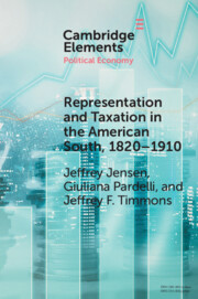
While the increase in property taxes between the mid-1840s and the onset of the Civil War that is apparent in Figures 4 and 6 may capture some of the need to finance debts, this period also coincided with a substantial increase across Southern states in public spending on railroads (Reference HeathHeath 1950; Reference FishlowFishlow 1965; Reference GoodrichGoodrich 1974). In turn, this period witnessed a sustained boom in the international demand for Southern cash crops that relied on enslaved labor, notably cotton. In both New Orleans and Liverpool, the primary international market for cotton, the price of “Middling American cotton” and sugar more than doubled between the mid-1840s and late 1850s. Tobacco prices in Liverpool rose more than threefold between 1843 and 1857 (Reference Gray and ThompsonGray and Thompson 1933, p. 492, 1026, 1033–1038). Figure 14 shows how the rising demand for Southern export crops affected commodity prices between 1840 and 1860. Specifically, Figure 14 (a) shows the five-year moving average of cotton prices in New Orleans from 1840 and 1860; Figure 14 (b) shows the five-year moving average of a commodity index reflecting variation in cotton, sugar, and tobacco prices over the same period.

Figure 14 Cotton prices ($) and Commodity Price Index, 1840–1860 (five-year moving average)
These price increases coincided with a production boom in these crops. Southern cotton production exceeded 2.2 billion pounds in 1860, up from less than 800 million in 1840. Sugar production also nearly tripled over this period (Reference Gray and ThompsonGray and Thompson 1933, p. 1033), while tobacco exports rose almost fivefold (Reference Gray and ThompsonGray and Thompson 1933, pp. 1033–1036).
Surging international prices and rapidly rising production enriched the relatively small group of Southern enslavers. For instance, the value of cotton exports rose from approximately $50,000,000 in 1846 to nearly $200,000,000 by 1860 (Reference NorthNorth 1960, p. 233).Footnote 51 As stated by Reference RansomRansom (2001), “There could be little doubt that the prosperity of the slave economy rested on its ability to produce cotton more efficiently than any other region of the world.” In turn, international demand for cash crops and the increased ability of Southern enslavers to meet this demand strongly influenced the value of their enslaved property. To wit, the late 1830s and 1840s depression in cotton prices was followed by declines in the average value of slaves, as captured by prices of major Southern slave auctions. As shown in Figure 15, the surge in international prices for cash crops was similarly followed by rapid increases in the value of slaves.

Figure 15 Average prices of enslaved persons
While the desire to meet rising international demand for these cash crops was clearly in enslavers’ economic interest, the limitations of the existing infrastructure network severely constrained their ability to do so. Millions of acres of otherwise fertile land went uncultivated due to their distance from navigable waters, rendering the use of expensive enslaved labor unprofitable. As was the case for non-slaveholders across the United States, substantial investments in infrastructure, such as canals and railroads, were necessary to connect vast amounts of potential farmland to markets. Furthermore, the lack of investment in infrastructure was an important source for Southern underdevelopment compared to the North (Reference WrightWright 2022).
One option for enslavers would be to finance the construction of railroads privately, as was the case in the UK and many of the Northern states. As we argued earlier, increasing the fiscal capacity of the states, as would be required to finance large-scale railroad construction, would be risky if the state government came to be controlled by the non-slaveholding majority. Yet privately financing the construction of railroad network on the scale required to unlock millions of remote and uncultivated potential farmland was completely infeasible: the costs and risks to private capital were far too high, and expectations of satisfactory returns were unlikely to be fulfilled in the sparsely populated and capital-poor South (Reference HeathHeath 1950; Reference FishlowFishlow 1965; Reference GoodrichGoodrich 1974; Reference LarsonLarson 2002).Footnote 52 According to Reference ReedReed (1962, p. 184), for example, “seventy-five per cent of the railroads chartered in the 1830s [in Louisiana] failed to materialize [due to constraints on capital].” More broadly, Reference LarsonLarson (2002, p. 239) claimed that the South was too “underdeveloped and incapable of supporting large-scale internal improvements on the strength of private fortunes alone.” The federal government was also not a viable solution; instead, public financing of infrastructure would need to come from Southern state and local governments (Reference Wallis and WeingastWallis and Weingast 2018). Unlike in the North, the South’s lack of large urban areas also meant that Southern state governments would need to be the primary source for public funding (Reference FishlowFishlow 1965, p. 397). As Reference MarrsMarrs (2009, p. 24) argues: “States proved to be a critical solution to the problem of railroad financing in the South.” Changes in infrastructure technology and international commodity markets meant that the economic interests of enslavers would be furthered by raising taxation on themselves to finance railroad construction. These large investments in public infrastructure financed by self-taxation would not only open up more land for cultivation but would also increase the demand for and the value of slaves, the primary asset of enslavers.
4.2 Variation in De Jure Political Control
We argue that Southern states in which enslavers had greater political control were more likely to respond to this rising demand for these crops by increasing property taxes on themselves in order to fund railroad construction that would further their economic interests. We exploit the fact that in seven of the fourteen states, representation in both chambers of the state legislature was systematically malapportioned in favor of higher slave-share districts (e.g., counties); representation in both chambers of the other seven Southern states was based on the principle of “one [adult White] man, one vote.” In the seven MS, the bias was due to: 1) representation based on total population including the enslaved, or capped representation that limited urban areas (e.g., Baltimore, New Orleans), 2) using the amount of taxes paid as the basis (which favored highly enslaved areas), or 3) the use of a fixed basis of representation, regardless of differences and changes in population. In the NMS, legislative representation was determined by each county’s White or eligible voter population, and required frequent reapportionment to capture spatial shifts in population.Footnote 53 The states that comprise the MS and the NMS are reported in Table 2. For each state, the table also shows the basis of representation in the legislature.
Table 2 Slave states and state legislative representation
| Basis of representation | ||
|---|---|---|
| Upper house (Senate) (1) | Lower house (H. of Rep.) (2) | |
| Malapportioned States (MS) | ||
| Florida | federal pop. | federal pop. |
| Georgia | fixed (1) | federal pop.* |
| Louisiana | total pop.* | total pop.* |
| Maryland | fixed (1) | total pop.* |
| North Carolina | taxation | federal pop. |
| South Carolina | fixed (1) | taxation |
| Virginia | fixed | fixed |
| Non-malapportioned States (NMS) | ||
| Alabama | White pop. | White pop. |
| Arkansas | White males | White males |
| Kentucky | qualified voters | qualified voters |
| Mississippi | White pop. | White pop. |
| Missouri | White pop. | White pop. |
| Tennessee | qualified voters | qualified voters |
| Texas | free pop. | free pop. |
Note: Federal population refers to the formula by which enslaved persons were counted as three-fifths of a person for the purposes of apportionment (as was the case with the US Constitution until the Fourteenth Amendment [1868]). An asterisk indicates states in which a maximum number of representatives/senators could be apportioned to any individual district. The number in parentheses denotes states in which each administrative district received an equal number of representatives/senators.
Legislative malapportionment provided a source of political power to enslavers. The economic geography of slavery meant that enslavers were typically spatially concentrated within each state.Footnote 54 Thus, systems of apportionment that overrepresented highly slave-dependent areas – whether by including slaves in the population count, basing representation on taxes paid, or using a fixed basis that overrepresented less populated rural areasFootnote 55 – could, despite their minority status, manufacture majorities for enslavers in the state legislatures.
The political power malapportionment provided was also enduring. This de jure electoral rule was “self-enforcing.” Because apportionment rules were enshrined in each state’s constitutions, the slaveholding elite need not expend resources to maintain them.Footnote 56 Furthermore, legislative majorities conferred by malapportionment allowed enslavers to block any equalizing reforms they opposed. Given this effective veto, it is unsurprising that none of the seven MS reformed their apportionment rules to a White-population basis. Legislative dominance was also critical in this period, as the other branches (the executive, the judiciary) were weak. Simply put, control of the state legislature meant control of the state government (Reference GreenGreen 1966; Reference ThorntonThornton 2014). In sum, malapportionment increased both the current power of enslavers and their expectation of future control.
Using malapportionment status to test our argument may lead to omitted variable bias if its adoption is not exogenous to the factors influencing taxation and spending on railroads. In each of the seven MS, this bias to legislative representation can be traced to the colonial era. Higher enslaved-share areas were overrepresented in colonial legislatures (Reference Pablo and JensenBeramendi and Jensen 2019), which was carried over into the initial postindependence constitutions (Reference GreenGreen 1966, pp. 97–98).Footnote 57 Simply put, disproportionate enslaver power was locked in long before the advent of railroads, as well as before the invention of the cotton gin and commercialization of cotton – Florida (1846) being the one exception. In the seven NMS, a population basis of apportionment was adopted in their initial constitutions and persisted throughout the antebellum period. The critical factor determining whether a new state adopted a biased basis of apportionment was whether the slaveholding elite was well established before statehood and able to implement this bias in the pre-statehood legislature (whether colonial or territorial).
This is not to say that enslavers in the NMS did not also possess disproportionate political power (e.g., Reference WoosterWooster 1969; Reference ThorntonThornton 2014). Rather, the consequence for enslavers in the NMS was that power was always more contestable. These elites had to consider whether the upside of more collective goods in the present period was worth the potential costs of political power in their now fiscally enhanced state being in the hands of the non-slaveholding majority.
Figure 16 shows the fourteen states by their malapportionment status and the share of their total population who were enslaved in 1860. While the average enslaved share in the MS (38 percent) exceeded that of the NMS (30 percent), there was great variation across both institutional groupings. Of the six states in which the enslaved share was greater than 40 percent – the so-called cotton states – two, Alabama and Mississippi, were non-malapportioned. In the five states whose enslaved share ranged between 20 percent and 40 percent of the total population, three were non-malapportioned. Of the three remaining “border” states – those with less than 20 percent enslaved share and who did not secede during the Civil War – one was malapportioned. Thus, the states are mostly balanced across this institutional feature at three very different levels of slave dependency.

Figure 16 Apportionment status and enslaved share (% of pop.), 1860
To further mitigate concerns about malapportionment status being correlated with other factors that could influence the association between commodity prices and taxation outcomes, in Figure 17 we conduct a balance test over a number of state-level characteristics that could predict the divergent fiscal trajectories we observe. The variables included in the balance test are: total population, enslaved population share, urban population share, state output, number of state officials PWC, and density of navigable rivers, as well as measures of agricultural suitability and production of cotton, sugar, and tobacco.Footnote 58 A statistically significant correlation between apportionment status and one of these covariates would suggest the presence of a potential alternative explanation for the decision of states to increase taxation. Different levels of cotton suitability between the MS and NMS, for example, would indicate that one group had more to gain from increasing taxation and investing in railroads than the other. Similarly, divergent cotton production levels in 1840 would suggest that some states benefited from greater productive capabilities when commodity prices began to rise. Differences in the initial stock of bureaucratic capacity may have allowed some states to raise taxes more rapidly than others, or created uneven incentives to invest in fiscal capacity (Reference Lee and PaineLee and Paine 2022). Finally, the density of navigable rivers also matters in that it may have made the need for railroads more pressing in some areas than in others. We find no statistically significant differences in any of these covariates across MS and NMS.

Figure 17 Balance test for pretreatment covariates, 1840
Note: Differences between (MS) and (NMS). Cotton, sugar, and tobacco suitability indices reflect the maximum potential yield based on climate, soil, and growing conditions as estimated by the UN Food and Agriculture Organization (FAO). Shares of urban and enslaved population; cotton, sugar, and tobacco production; and state output are measured in 1840. Density of navigable rivers (representing the total length of rivers over the surface area of each state) is obtained from Reference AtackAtack (2015); and the share of public officials PWC is measured in 1850 (no prior census provides this information). See Table B4 for more details on sources.
In short, circa 1840, our comparison states had roughly similar endowments. They differed primarily on the supply side: in half of the states, the slaveholding elite’s power to control taxes and public spending was substantially less contested in both the present period and for the foreseeable future; in the other half, their control was less certain. Whereas the commodity boom increased the value of land and slaves, and infrastructure bottlenecks constrained those assets from reaching their full potential across both the MS and NMS, only the elite in the MS had the power and incentive to use their secure hold on power to tax themselves to finance collective goods that would leverage the boom for their benefit. We thus expect tax and spending differentials to emerge across the two types of states, with the MS increasing the incidence of taxation on their elites and public spending on railroads at a faster clip than their NMS counterparts.
4.3 Results
We begin with visual evidence that rising commodity prices translated into a greater rise in property taxes in the MS compared to the NMS. Figures 18 and 19 show the trend in the average property taxes PWC (1820–60) and as a share of output (1840–60), respectively. Although both follow largely similar trajectories until the early 1840s, they quickly and noticeably diverge when commodity prices begin to increase, as predicted. Since these differences could, in theory, be driven by distinct levels of state capacity or uneven patterns of economic growth, in Figure 20 we examine the trends in ad valorem property tax rates over the same period.Footnote 59

Figure 18 Property taxes/White population (real $), 1820–1860 Malapportioned versus non-malapportioned states

Figure 19 Property taxes/agricultural and manufacturing output, 1840–1860 Malapportioned versus non-malapportioned states

Figure 20 Property tax rates, 1840–1860 Malapportioned versus non-malapportioned states
To evaluate whether changes in commodity prices disproportionately affect property taxes in the MS during this period, our empirical strategy adopts the following difference-in-differences approach:Footnote 60
 (1)
(1)where
 is a state-level measure of property tax revenues or ad valorem rates, for state
 at time
 .
.
 is an indicator variable that takes the value 1 if the state legislature of state
 is malapportioned in year
 , and 0 otherwise. Our main variable of interest
 reflects cotton prices (logged) in year
 . The parameter
 captures the differential effect of commodity prices on property taxes in the MS. Both dependent and independent variables are measured as three-year moving averages to reduce small fluctuations.
 represents a vector of time-varying covariates;
 and
and
 are respectively state and year fixed effects, and
 is an error term.
Table 3 shows our benchmark models investigating the effect of apportionment status and commodity prices on total state property taxation PWC without any additional covariates. The second column includes time-varying controls, namely total population (log), urban population (log), and total output (log). The third column includes the same covariates, but measured in 1840, to minimize potential concerns about posttreatment bias, and interacted with year indicators. The estimates are substantively similar across specifications. The positive and significant interaction term between apportionment status and cotton prices captures the predicted moderation effect. As expected, an increase in international commodity prices differentially affects tax revenues in the MS, where elites have full control of the state apparatus.Footnote 61 To address the concern that cotton prices might be endogenous, in Appendix Table A1, we adopt an alternative measure for our independent variable, a commodity price index weighted by the relative suitability of each state to the cultivation of three main crops: cotton, sugar, and tobacco. This measure reflects the exposure of states to fluctuations in international commodity prices at any given point in time based on their suitability to the cultivation of each crop relative to the Southern average. We also evaluate the possibility that coastal status and access to the Mississippi River might correlate with malapportionment and explain our results (see Table A2). Our substantive results remain unchanged.
Table 3 Antebellum period: Property taxes, cotton prices, and malapportionment status
| Dependent variable | |||
|---|---|---|---|
| Property taxes per White capita (real $) | |||
| (1) | (2) | (3) | |
Cotton prices

| 2.057 *** | 1.959 *** | 2.087 *** |
| Malapportionment | (0.631) | (0.565) | (0.605) |
| State fixed effects | Yes | Yes | Yes |
| Year fixed effects | Yes | Yes | Yes |
| Geographic controls | Yes | Yes | Yes |
| Time-varying covariates | No | Yes | No |
| Time-invariant covariates | No | No | Yes |
| Observations | 268 | 268 | 259 |
R

| 0.429 | 0.476 | 0.623 |
Note: Main variables measured as three-year moving averages. Geographic controls are: state area, cotton suitability, and river density. These covariates are interacted with year indicators. Time-varying covariates are: state population (log), urban population share, and log of total output (agriculture and manufacturing). Column 1 includes geographic controls only; column 2 includes geographic controls and time-varying covariates. Column 3 includes the same covariates measured in 1840 (pretreatment) interacted with year indicators. * p
 0.1; ** p
 0.05; *** p
 0.01.
0.01.
Figure 21 shows that poll tax rates do not follow the same pattern: there is no difference in either levels or trends across the two groups of states. In fact, this figure indicates that unlike property taxes, regressive poll taxes did not rise in the MS. Consistent with Reference Thornton, J. Morgan Kousser and JamesThornton’s (Reference Thornton, J. Morgan Kousser and James1982) assessment that the wealthiest third of the citizenry paid at least two-thirds of all taxes during the antebellum period, these results suggest that elites in the MS financed state-level fiscal expansion by taxing themselves, eschewing taxes that fell more heavily on the non-slaveholding White majority.

Figure 21 Poll tax rates, 1840–1860 Malapportioned versus non-malapportioned states
4.4 Collective Goods for Elites: Railroads versus Education
A critical aspect of our argument is that economic elites will support increasing taxation on themselves if this revenue funds collective goods that enhance their interests. We now turn to railroad construction and trends in public education; the former disproportionately favored elites, while the latter, presumably, disproportionately benefited the average White citizen.Footnote 62
To measure public support for railroads, we rely on data presented by Reference HeathHeath (1950), who collected all public (federal, state, and local) spending on railroads in the South prior to 1861. In total, at least $144 million of public funds were spent constructing railroads in these states prior to 1861 (out of $252 million total [public and private] spending on railroads in the South [Reference FishlowFishlow Reference Fishlow1965, p. 397]).Footnote 63 Of the public total, 57 percent of this came from state governments.Footnote 64
We create three measures of state public spending on railroads, presented in Table 4. Column 1 shows total spending on railroads by state governments in this period as a proportion of each state’s White population in 1860. On average, state government spending on railroads is approximately six times higher PWC in the MS. Column 2 normalizes state spending on railroads by state income in 1860. Even when normalized by income, MS governments spent three times more. Column 3 reports the share of public spending on railroads that comes from state sources. In the states in which enslavers had much greater control of state governments we see a much higher proportion of public spending occurring at the state level. Columns 4 and 5 provide railroad mileage data from Reference AtackAtack (Reference Atack2015), allowing us to assess the possibility that public spending on railroads merely cloaks rent-seeking corruption by elites in the MS. Whether normalizing total railroad mileage by White population (column 4) or state income (column 5), the MS created significantly more railway mileage on average, indicating that public funds translated into output and did not solely line the pockets of governing elites.
Table 4 Collective goods: State support for railroads, 1860
| State Government Railroad Spending Railway Mileage | |||||
|---|---|---|---|---|---|
| Railroad spending PWC ($) (1) | Railroad spending sh. income (%) (2) | State sh. public RR spending (%) (3) | Railway mileage PWC (4) | Railway mileage sh. income (%) (5) | |
| Malapportioned | |||||
| Florida | 62.7 | 39.0 | 89.4 | 0.52 | 0.003 |
| Georgia | 11.7 | 7.8 | 53.9 | 0.24 | 0.002 |
| Louisiana | 9.5 | 3.7 | 38.7 | 0.09 | 0.004 |
| Maryland | 0.07 | 0.006 | |||
| North Carolina | 16.9 | 13.6 | 89.3 | 0.14 | 0.001 |
| South Carolina | 33.2 | 17.2 | 70.6 | 0.34 | 0.002 |
| Virginia | 22.7 | 18.6 | 75.0 | 0.17 | 0.002 |
| AVERAGE | 30.6 | 16.7 | 72.0 | 0.22 | 0.003 |
| Non-malapportioned | |||||
| Alabama | 4.1 | 3.0 | 36.6 | 0.14 | 0.001 |
| Arkansas | 0.6 | 0.4 | 47.4 | 0.02 | 0.000 |
| Kentucky | 0.8 | 0.8 | 4.5 | 0.06 | 0.001 |
| Mississippi | 6.0 | 2.1 | 50.8 | 0.25 | 0.001 |
| Missouri | 6.6 | 6.6 | 0.08 | 0.001 | |
| Tennessee | 20.9 | 20.7 | 66.9 | 0.14 | 0.001 |
| Texas | 0.0 | 0.0 | 0.0 | 0.07 | 0.001 |
| AVERAGE | 5.9 | 5.0 | 34.3 | 0.11 | 0.001 |
Note: Railroad spending comes from Reference HeathHeath (1950). Railway mileage was obtained from Reference AtackAtack (2015). PWC indicates per White capita.
One concern is that we might be simply capturing demand side variation (e.g., Reference Lee and PaineLee and Paine 2022) – rather than, as we argue, political supply. Our evidence suggests this is unlikely. First, as our balance and robustness tests illustrate, we fail to confirm that the geography of the NMS meant they needed fewer railroads. Second, a large historical literature has shown that strong demand for railroads existed across the South (e.g., Reference HeathHeath 1950; Reference GoodrichGoodrich 1974; Reference LarsonLarson 2002). The problem of political supply rather than demand is demonstrated, for example, by Reference ThorntonThornton (2014, p. 107), who notes the difficulty of receiving public financing in highly enslaved, but not malapportioned, Alabama: “Time and again, when a small loan or expenditure could have added millions of dollars to the commerce of the state by facilitating trade, the legislature refused to act.” Third, we look at railroad miles by state in 1880, roughly ten years after Congress completely altered the political system of Southern states with Reconstruction. As evidence that state-specific demand-side factors cannot explain the large differences in prewar railroad supply, we observe no meaningful difference on average across MS and NMS in railroad mileage as a share of income (0.0029 vs. 0.0025,
 ) and mileage PWC (0.23 vs 0.19,
 ) in 1880.
Public Education Spending
We now turn to public education, a redistributive good that would have been much more favored by the wider electorate. The 1860 Census provides several measures of state-level support for public education, such as the sources of public financing for public and private schools, and White school attendance in public and private schools. We normalize this information with the White school-aged population (ages five to fourteen) and state income to create measures of enrollment rates and expenditures. Table 5 reports average spending and enrollment figures for MS (column 1) and NMS (column 2).
Table 5 State support for redistribution: Public education, 1860
| Malapportioned States (average) (1) | Non-malapportioned States (average) (2) | |
|---|---|---|
| Panel A: School Attendance | ||
| Whites attending school / | 56.4 | 63.4 |
| Whites, 5–14 (%) | ||
| White public school pupils / | 32.4 | 43.6 |
| Whites, 5–14 (%) | ||
| White public school pupils / | 74.8 | 85.8 |
| Total pupils (%) | ||
| Panel B: State Government Spending | ||
| State public school spending / | 0.72 | 0.89 |
| Whites, 5–14 ($) | ||
| State public school spending / | 2.12 | 2.06 |
| public school pupils ($) | ||
| State total educ. spending / | 3.39 | 2.4 |
| public school and private pupils ($) | ||
Note: All variables were constructed from the 1860 US Census. Each value is the average across the states in the MS (column 1) and NMS (column 2).
Panel A focuses on white school attendance, especially in public schools. As is evident, a greater share of White school-aged children attended school in the NMS (63 percent) than in the MS (56 percent). The census also asked state superintendents to report the number of pupils in public and private schools, respectively.Footnote 65 We thus construct two measures of state reliance on public schools: White public school pupils as a share of each state’s White school-aged population and the share of total pupils (private and public school) in public schools. With both measures, the average is higher in the NMS.
Panel B focuses on state government education spending for both public and private schools. First, we compare state government spending on public schools as a share of the state’s White population, ages five to fourteen. On average, it is slightly higher in the NMS (eighty-nine cents per school-aged White person versus seventy-two cents). Next, we calculate state government support as a proportion of public school pupils. Although the MS had a greater share of students in private schools, state government spending per public school pupil was almost identical ($2.12 in the average MS versus $2.06 in NMS). The census data also allow us to construct measures of total public spending per public and private school pupil. Despite private school enrollment comprising only roughly 25 percent of total pupils in the MS, private schools received on average roughly 40 percent of state education funding. In other words, despite significantly higher taxes, the average MS did not provide more support for public education; instead, they funneled more public money toward private education. In sum, none of these measures show differences across the MS and NMS in public education supply that are remotely comparable to the gaps observed in public support for railroads.
4.5 Robustness
In the Appendix, we evaluate the robustness of our results. To minimize concerns that property taxes may be rising mechanically due to differential changes in the intensity of slavery across states, Appendix Table A3 includes the size of the enslaved population as an additional covariate in our baseline specifications. Our coefficients of interest remain largely unchanged while the size of the enslaved population has a negative (albeit not always significant) association with property taxes.Footnote 66 In Appendix C, we discuss endogeneity concerns with malapportionment, and we consider whether omitted factors may explain both malapportionment and the observed increase in property taxes in the late antebellum period. Similarly, in Appendix D, we address concerns that initial differences in state capacity may have been responsible for the uneven increase in taxation across states. We also use county-level collection of state taxes to demonstrate that greater taxes did indeed fall on the counties with higher shares of enslaved population.
5 Postwar Taxation
5.1 Reconstruction and Its Aftermath
5.1.1 Context
In the aftermath of the North’s victory in the American Civil War and the Thirteenth Amendment’s emancipation of nearly 4 million enslaved Americans, congressional Republicans sought to permanently weaken Southern rural elites’ stranglehold on political power with the passage of the Military Reconstruction Acts of 1867 and 1868 (Reference FonerFoner 2014).Footnote 67 These acts, as a condition for regaining their seats in Congress, required ten former Confederate states to create new state constitutions granting universal adult male suffrage and to ratify the Fourteenth Amendment, which enshrined the principle of civil rights and equal protection under the law for all citizens.Footnote 68 Perhaps just as important, these acts also required the army to register adult Black males to vote and to protect their ability to exercise the franchise and run for office.
These reforms resulted in a temporary transformation of the party system, and the distribution of political power more broadly, in these ten Southern states. Immediately following the adoption of new state constitutions, which extended the franchise to all adult males, the Republican Party, which was nonexistent in the prewar South, won nine gubernatorial elections and majorities in seventeen legislative chambers (Reference DubinDubin Reference Dubin2007, Reference Dubin2010). The Republican Party’s initial success was driven by Black voters, who formed the backbone of the party in the South. The effectiveness of these reforms was demonstrated by the election of thousands of Black politicians and officials to local, state, and federal office throughout the South in the decade following passage of the Military Reconstruction Acts (Reference FonerFoner 1993).
This political revolution resulted in a substantially expanded role for the Southern states in providing redistributive public goods. According to Reference FonerFoner (2014, p. 364), “Serving an expanded citizenry and embracing a new definition of public responsibility, Republican government affected virtually every facet of Southern life … Public schools, hospitals, penitentiaries, and asylums for orphans and the insane were established for the first time or received increased funding.” Most dramatically, Republicans fundamentally altered the role of the state with regards to providing a public education for all children (Reference FonerFoner 2014, p. 366). This new redistributive spending was financed primarily by increasing property taxes on the landed elite (see Figures 4 and 6).Footnote 69
Rising property taxes thus became an effective rallying cry for opponents of Reconstruction. Democratic leaders in many states soon organized taxpayers’ conventions, where participants expressed their objection not only to the claimed profligacy of Reconstruction government but to the new purposes of public spending, such as the financing of common schools. Convinced that the increasing tax burden resulted from the fact that “nine-tenths of the members of the Legislature own no property and pay no taxes” (Reference FonerFoner 2014, p. 416), Democrats called for a return to rule by property holders, which entailed denying Blacks, as well as many Whites, any role in government.
The powerful backlash in response to radical changes in government was not confined to taxpayers’ conventions. It also took the form of political violence, the intensity of which can scarcely be dissociated from fiscal policy: as shown by Reference LoganLogan (2019), Black officeholders in locations with higher taxes were more likely to be victims of attacks. In addition to the use of the US Army to suppress this violent counterrevolutionary reaction, Congress responded by passing the three Enforcement Acts empowering the newly created Department of Justice to regulate state and local elections, enforce political and civil rights, and prosecute those who impeded political participation. Through its expanded authority, the federal government was able to successfully prosecute more than 1,000 violations between 1871 and 1874, and to temporarily constrain non-state violent groups such as the Ku Klux Klan (Reference Walton, Puckett and DeskinsWalton et al. 2012).
While Radical Reconstruction was briefly successful at overturning the existing political structure in these states, little was done to remedy the vastly unequal ownership of economic assets, in particular land. Despite much debate, no program of land redistribution was adopted. As a result, landownership remained highly concentrated, especially in the former plantation counties where most of the Black population lived. We argue that the persistence of this massive inequality in economic resources meant that the ability of Blacks to successfully use their newly granted political rights to influence social and economic policies required constant federal intervention on their behalf. But the federal intervention, especially in terms of the military occupation, was spatially uneven and declining in scope over time.Footnote 70
There was also significant spatial and temporal variation in the extent to which Reconstruction was successful, as measured by the victories of the Republican Party. This variation leads to our main prediction regarding the incidence of property taxes during Reconstruction and its immediate aftermath. In five Reconstruction states – Arkansas, Florida, Louisiana, Mississippi, and South Carolina – the Republican Party was able to win unified control of the state government (legislature and governor’s office) for multiple electoral cycles in a row. South Carolina, for instance, even had a majority-Black state legislature from 1868 until 1876. We call these five Reconstruction states Republican Control states. We argue that this control demonstrates that federal intervention, even if only briefly, limited the ability of Southern elites to use their de facto power to overcome majoritarian preferences when de jure political rights are effectively enforced. Despite considerable resistance, with the federal government subsidizing the cost of enforcement, we expect property taxes on elites to rise and remain high as long as this “democracy by the gun” persists.
The federal government’s ability to protect Black voters across the entire South was never fully realized. In the other five Reconstruction states – Alabama, Georgia, North Carolina, Texas, and Virginia – the Republican Party never gained a stronghold. Following the first set of Reconstruction elections, the Democratic Party always held at least one chamber of the legislature or the governor’s office until the Democratic Party regained complete control. We call these five states the Mixed Control Reconstruction states. In these states, where the Democratic Party always retained enough power to protect planters, we do not expect taxation to rise much at all, and certainly to be significantly lower than in the five Republican Control Reconstruction states.
Last, we call the four Southern states that were not subject to the Reconstruction Acts (i.e., were not placed under military rule, were not required to write new state constitutions, retained federal representation) the non-Reconstruction states. As with the Mixed Control states, we do not expect property taxes to increase in non-Reconstruction states during the Reconstruction period.
The federal government’s ability to enforce Black political rights in the South fell precipitously following the congressional elections of 1874, as Democrats won a majority in the federal House of Representatives for the first time since the onset of the Civil War. Democrats used this majority to block further military appropriations for Reconstruction.Footnote 71 The Compromise of 1877, which gave the Republicans the presidency in exchange for, among other promises, a commitment to remove troops engaged in enforcing Reconstruction, ended the remaining federal efforts to protect Black voters (Reference FonerFoner 2014). The end of any federal commitment to enforce Black political rights coincided with the loss of political control by Republicans in the last few Reconstruction states (e.g., Florida, South Carolina) and with the slow convergence of property taxation across all three sets of states.
Our argument predicts that under the conditions observed in the post-Reconstruction period, we should no longer see increases in property taxes. While Southern elites, through the Democratic Party, regained power, especially relative to Reconstruction, their hold on power remained contested and future political control was uncertain. Although substantially weakened by the increasingly unfettered ability of Southern Democrats to use violence and electoral fraud, Blacks formally retained the franchise and in practice remained politically active (Reference KousserKousser 1974; Reference Tolnay and BeckTolnay and Beck 1995). Non-Democratic candidates and parties still contested and occasionally even won elections in some states in the immediate post-Reconstruction period (1877–90). Furthermore, federal politics could shift in a way that supported interventions to enforce Black political rights. In this setting of contested and uncertain control on power, we expect that elites will not have incentives to support increases in property taxation.
At the same time, the coercive taxation framework predicts that in the absence of external enforcement, not only are tax increases unlikely, but we should actually see a collapse in the ability of the state to extract. This is precisely what we observe with the end of federal intervention, when property tax rates in occupied states reverted to pre-Reconstruction levels.Footnote 72
5.1.2 Analysis
We again start with graphical evidence of our claim that on average the military occupation of the ten Reconstruction states (RS) led to higher progressive property taxation than what was observed in the four non-Reconstruction states (NRS). We then distinguish between states where the Republican Party gained unified political control and those where party control was mixed, in order to evaluate whether these groups displayed differential trajectories.
We first examine whether the presence of federal troops affected property tax trends. Figures 22 and 23 respectively present property taxes PWC and as a share of output, and Figure 24 presents ad valorem rates across the ten RS and four NRS. The vertical lines show the year in which the Democratic Party regained unified control in each state (i.e., “Redemption” in the language of Southern Democrats). As these figures illustrate, although both groups started off with similar levels of taxation in the immediate aftermath of the war, property taxes rose substantially more among the Reconstruction states, while trends remained relatively stable over time in comparison states.

Figure 22 Property taxes per White capita (real $), 1868–1880 Reconstruction versus non-Reconstruction states (three-year moving average)

Figure 23 Property taxes/total output (agriculture and manufacturing), 1868–1880 Reconstruction versus non-Reconstruction states (three-year moving average)

Figure 24 Property tax rate, 1868–1880 Reconstruction versus non-Reconstruction states (three-year moving average)
We now separate states into three groups: the five Republican Control Reconstruction states, five Mixed Control Reconstruction states, and four non-Reconstruction states. Their trajectories are shown in Figures 25, 26, and 27. In accordance with our theoretical expectations, almost all of the increase in property taxes observed among Reconstruction states in the previous figures can be attributed to the five states in which Republicans were able to achieve unified political control for multiple consecutive electoral cycles.

Figure 25 Property taxes per White capita (real $), 1868–1880 by Reconstruction status and party control (three-year moving average)

Figure 26 Property taxes/total output (agricultural and manufacturing), 1868–1880 by Reconstruction status and party control (three-year moving average)

Figure 27 Property tax rate, 1868–1880 by Reconstruction status and party control (three-year moving average)
To further investigate the association between Reconstruction status and property taxation between 1868 and 1880, we adopt the following two-way fixed-effects model:
 (2)
(2)where
 is a state-level measure of property tax revenues or ad valorem rates, for state
 at time
 .
.
 is an indicator variable that takes the value 1 if state
 is occupied by federal military forces in year
 , and 0 otherwise. Both dependent and independent variables are measured as three-year moving averages.
 represents a vector of time-varying covariates, while
 and
and
 represent state and year fixed effects.
Table 6 presents our baseline results for this period. As our theory predicts, federal intervention is associated with a significant increase in property taxes PWC. Table 7 further breaks down this result by differentiating between the five Republican Control states (i.e, where Republicans had unified control [governor plus both chambers of the legislature] for several consecutive electoral cycles), and the five Mixed Control Reconstruction states (i.e., those where the Republican Party lacked unified control for consecutive cycles).Footnote 73 To assuage concerns that the Reconstruction variable may simply be picking up variation in the proportion of the newly enfranchised electorate across states, all specifications account for the share of the enslaved population in 1860. As the results show, the effect of Reconstruction on property taxes is much greater in states where the elite-dominated Democratic Party was fully removed from power than in those states where Democrats were still able to formally influence policymaking.
Table 6 Postwar period: Property taxes and Reconstruction status
| Dependent variable | |||
|---|---|---|---|
| Property taxes per White capita (real $) | |||
| (1) | (2) | (3) | |
| Reconstruction Status | 0.385 * | 0.407 *** | 0.421 ** |
| (0.204) | (0.155) | (0.209) | |
| State fixed effects | Yes | Yes | Yes |
| Year fixed effects | Yes | Yes | Yes |
| Geographic covariate | Yes | Yes | Yes |
| Time-varying covariates | No | Yes | No |
| Time-invariant covariates | No | No | Yes |
| Observations | 306 | 306 | 306 |
R

| 0.332 | 0.474 | 0.521 |
Note: Dependent variable measured as three-year moving average. All specifications account for share of enslaved population, state area, and population size (log) in 1860. Time-varying covariates included in column 2 are: state population (log), urban population (log), and agricultural and manufacturing output (log). Column 3 includes the same covariates measured in 1860 (pretreatment) interacted with year indicators. We test for the potential influence of negative weights, as proposed by Reference de Chaisemartin and D’Haultfoeuillede Chaisemartin and D’Haultfoeuille (2020), and find that all of our ATT receive a positive weight. * p
 0.1; ** p
 0.05; *** p
 0.01.
0.01.
Table 7 Post Civil War period: Property taxes, Reconstruction status, and party control
| Dependent variable | |||
|---|---|---|---|
| Property taxes per White capita (real $) | |||
| (1) | (2) | (3) | |
| Reconstruction and |
 0.164
0.164 | 0.111 |
 0.027
0.027 |
| Mixed Party Control | (0.265) | (0.139) | (0.171) |
| Reconstruction and | 1.054 *** | 0.802 *** | 1.236 *** |
| Full Republican Control | (0.359) | (0.296) | (0.291) |
| State fixed effects | Yes | Yes | Yes |
| Year fixed effects | Yes | Yes | Yes |
| Geographic covariate | Yes | Yes | Yes |
| Time-varying covariates | No | Yes | No |
| Time-invariant covariates | No | No | Yes |
| Observations | 306 | 306 | 306 |
R

| 0.422 | 0.495 | 0.596 |
Note: Dependent variable measured as three-year moving average. All specifications account for share of enslaved population, state area, and population size (log) in 1860. Time-varying covariates included in column 2 are: state population (log), urban population (log), and agricultural and manufacturing output (log). Column 3 includes the same covariates measured in 1860 (pretreatment) interacted with year indicators. The omitted category is Non-Reconstruction. Wald tests reveal that we can reject the null hypothesis that the coefficients for Mixed and Full Republican control are equal. * p
 0.1; ** p
 0.05; *** p
 0.01.
0.01.
One obvious question regards what drove Republican control across states. Reference Chacón, Jensen and YntisoChacón et al. (2021) show, using a county-level panel, that for a given set of structural characteristics that shaped demands for redistribution (including the size of the formerly enslaved population), the local proximity of federal troops increased the electoral success of Republican state legislators. In Appendix Table A4, we show that this pattern also holds at the state level.
A related concern is that our analysis may suffer from omitted variable bias. Reference Suryanarayan and WhiteSuryanarayan and White (2021), for example, have shown that within Confederate states, the hollowing out of the state’s administrative apparatus in the post-Reconstruction period was stronger in formerly high-slavery counties where intra-White inequality was higher. To account for the possibility that these two factors varied systematically with Republican Party control within the Confederate sample, we include both the share of the enslaved population in 1860 and intra-White inequality in 1850 as covariates, which we interact with year indicators to capture differences in trajectories across states (Table A5). Our results remain unchanged, suggesting that slavery, intra-white inequality, and Republican control influenced taxation outcomes through independent channels.
A final concern might be that the observed patterns reflect different trends in overall revenues across states, rather than an expansion in elite taxation. Using the same approach we used to investigate this possibility during the antebellum period, we look at the trajectories of poll taxes across RS and NRS. As Figure 28 shows, there is no evidence of significant changes in non-property taxation across both groups of states during this period.

Figure 28 Poll tax rate, 1868–1880 Reconstruction versus non-reconstruction states
5.1.3 State Spending on Common Schools
Last, we provide evidence that RS and, in particular, states with full Republican control, not only levied significantly higher property taxes during the occupation period, but they also spent significantly more on redistributive public goods preferred by Blacks and poorer Whites. As with property taxes, we expect spending in these states to decline with the end of Reconstruction. Given the absence of significant political changes in the NRS, and the contested nature of political power in the Mixed Control states, we should observe less variation in education spending during or after the end of Reconstruction across these two groups.
To test this argument, we collect the amount of either state taxes devoted to common schools or state spending from general revenues allocated toward public schools annually between 1870 and 1910, taken from state reports of the superintendent of public education (see Appendix B for sources).
Figure 29 illustrates the trends in state taxes allocated to common schools across RS and NRS. State revenues devoted to common schools as a share of output expanded markedly throughout the first half of the 1870s among the states that underwent Reconstruction, only to fall abruptly following removal of federal troops.Footnote 74

Figure 29 State taxation for common schools/total output, 1870–1880 Reconstruction versus non-Reconstruction states (three-year moving average)
In Figure 30, we distinguish between states where the Republican Party had unified control of state government for consecutive terms and those where the Democratic Party retained some representation. The evidence is consistent with the theoretical expectation that fiscal resources devoted to common schools as a share of output saw a substantial increase in states dominated by the Republican Party, while remaining largely unchanged in the other two groups of states. With the end of federal Reconstruction, however, this exceptional bout of growth was replaced by a period of steep decline in state school revenues among RS, which again contrasts with the trends observed in the NRS and Mixed Control states, where school taxes as a share of output remained generally stable during the same period.

Figure 30 State taxation for common schools/total output, 1870–1880 by Reconstruction status and party control (three-year moving average)
5.2 Jim Crow: Formal Black Disenfranchisement (1880–1910)
5.2.1 Context
While the redistributive threat posed by the Republican Reconstruction governments had been eliminated by 1877, adult Black males formally retained the right to vote. In the years after Reconstruction, non-Democratic Party candidates for governor and the state legislature continued to receive substantial shares of the vote in many Southern states.Footnote 75 Of particular concern to Southern elites, cross-racial class-based (“fusion”) coalitions had successfully formed to win control of state governments in Virginia (early 1880s) and North Carolina (mid-1890s), and had nearly won in several other states (Reference PermanPerman 2003).
While the durability of such coalitions was never demonstrated during this period, the mere possibility posed a particular threat to Southern elites. Like many rural societies based on coerced labor, the US South during the 1880s was characterized by high land inequality, fiscal retrenchment, and low spending on broad public goods, especially public education (Reference Alston and FerrieAlston and Ferrie 2007; Reference MargoMargo 2007; Reference Galor, Moav and VollrathGalor et al. 2009; Reference VollrathVollrath 2013; Reference Suryanarayan and WhiteSuryanarayan and White 2021). The increase in regressive taxation and retrenchment in public spending that emerged in the post-Reconstruction period engendered significant resentment among poorer Whites and fueled the populist and cross-racial fusion movements that threatened Southern Democratic Party dominance (Reference KousserKousser 1974; Reference HymanHyman 1989; Reference HahnHahn 2006).
These electoral threats to Democratic Party rule ended with the adoption by eleven states of various suffrage restrictions, such as poll taxes and literacy tests, between 1889 and 1906 (Reference PermanPerman 2003; Reference ValellyValelly 2009).Footnote 76 While not explicitly racial in nature, these restrictions removed the formal voting eligibility of substantial portions of the Black electorate.Footnote 77 The historical record is clear that elites saw White supremacy as crucial for maintaining Democratic Party hegemony. To take just one example, a delegate to the 1898 Louisiana constitutional convention, which adopted poll taxes and a literacy test, said: “What is the state? It is the Democratic Party … We meet here to establish the supremacy of the white race, and the white race constitutes the Democratic Party of this state.” The effects of these restrictions on lower-income Whites is less known. While ‘Grandfather’ clauses and other similar mechanisms were adopted to maintain White voter suffrage, turnout and likely voter eligibility of lower-income Whites declined (Reference KousserKousser 1974).
Our argument suggests that in the post-Reconstruction period, during which political contestation to Democratic Party elite rule remained and future control was uncertain, we should expect declining and/or low levels of progressive property taxation. If franchise restrictions led to tighter elite control and elites demanded some collective goods, we should see that Black disenfranchisement resulted in higher property taxes. If, however, elite control was not coupled with demands for greater collective goods, then taxation should not rise much. As shown in what follows, states in which elite control was strongest – as measured separately by either the implementation of a literacy test (which disenfranchised most Black voters) or the Democratic Party seat share in the state legislature – had higher property taxes PWC. Spending, however, does not increase to the same extent as in the prewar period. We believe there were fewer collective goods desired by elites at this time, something that would not change appreciably until the automobile age. The key point in terms of our argument is that property taxes and spending on elite goods, such as colleges and universities, increased more in states in which the Democratic Party had greater control.
5.2.2 Analysis
We begin by visually showing the change in property taxes between 1880 and 1910 across states that adopted some type of suffrage restriction (poll tax or literacy test) versus those that did not enact any of these measures. This allows us to assess if the patterns observed among disenfranchising states diverge from the secular trends affecting all states irrespective of their voting laws.
Each category separates the states into the likely effects of Black disenfranchisement on elite political control. Literacy tests and poll taxes drastically reduced the political participation of Black voters and therefore should have provided elites with a higher degree of political control both in the present and into the future. By contrast, the absence of suffrage restrictions clearly did little to institutionally buffer elite dominance. Holding elite demand for collective goods constant, we expect property taxes in the states with poll taxes or literacy tests to increase faster (or fall less) than in the states without voting restrictions.Footnote 78
Figure 31 shows the average property taxes PWC and as a share of output, along with ad valorem rates, for each set of states between 1880 and 1910. The dashed vertical lines in these figures denote the year in which each state adopted voting restrictions (either a poll tax or a literacy test). As the first figure shows, property taxes PWC increased rapidly, on average, among states that implemented suffrage restrictions and remained largely unchanged in comparison states. As a share of output (Figure 31b), property taxes fell markedly and continuously among non-Restriction states while showing a less pronounced decrease among disenfranchising states. In particular, the acceleration observed in the years after the last state (Georgia) implemented restrictive measures does not appear to be driven by common shocks affecting all states: there is no increase in states that did not adopt voting restrictions.


Figure 31 Property tax outcomes by restriction status, 1880–1910
While the amount of property taxes levied constitutes a common measure of direct taxation on the wealthy, it may reflect both a political decision and underlying differences in states’ fiscal capabilities. Because our theory seeks to explain supply-side decisions, changes in ad valorem property tax rates provide a strong complementary test. We present these results in Figure 31c. The striking divergence is consistent with our previous findings and strengthens the credibility of our other taxation measures.
Another way of evaluating the existence of differential trends across groups of states is to look at taxation patterns based on the number of years from the implementation of suffrage restrictions. Given the staggered adoption of disenfranchising measures across states, such figures may provide a clearer depiction of the incremental divergence between Restriction and non-Restriction states. Figure 32 shows, in Black, average property taxes among states that implemented voting restrictions in the ten years before disenfranchisement and the twenty years after. The grey lines show property taxes in states that did not adopt restrictive measures. Once again, the figures show a marked divergence in property taxes between states that adopted franchise restrictions and the comparison group.Footnote 79


Figure 32 Property tax outcomes by disenfranchisement status ten years before and twenty years after suffrage restrictions
Note: The black lines show average (a) property taxes PWC, (b) as a share of output, and (c) ad valorem rates across states that adopted suffrage restrictions. For each state where voting restrictions were implemented in a given year, we calculate the average property taxes of a control group that is composed of all states that did not have restrictive measures in that year or before – i.e., the control group includes both never-treated and not-yet-treated units. The grey line reflects the average trend across all control groups.
To further assess our hypothesis that variation in elite control is the relevant mechanism through which poll taxes and literacy tests may influence property taxation, we investigate the heterogeneous effects of suffrage restrictions with respect to the level of political dominance that the Democratic Party achieved across states. Specifically, we differentiate between states where the Democratic Party had a high (i.e., above average) share of seats in the state legislature following the adoption of restrictions and those where the party’s dominance was less pronounced – Arkansas, North Carolina, Tennessee, and Virginia – despite having adopted the same measures as their counterparts.
We present property taxes PWC across time by level of Democratic control in Figure 33, property taxes over output in Figure 34, and ad valorem tax rates in Figure 35. The diverging lines suggest a significant gap in taxation between the disenfranchising states where the Democratic Party dominated the legislature and both states without restrictions and those with voting restrictions but weaker Democratic control. Although the three groups display largely parallel trends before 1890, their taxation patterns begin to diverge after the first states (Florida, Mississippi, and Tennessee) adopt franchise restrictions. Overall, the figures show that Democratic-leaning states appear to experience a larger increase in property taxes PWC – and a smaller decrease in property taxes over output – than their counterparts, which we attribute to elites’ increased political control and reduced uncertainty over their future ability to shape fiscal policy in these states.

Figure 33 Property taxes per White capita (real $), 1880–1910 by disenfranchisement status and Democratic seat share (three-year moving average)

Figure 34 Property taxes/output, 1880–1910 by disenfranchisement status and Democratic seat share (three-year moving average)

Figure 35 Property tax rate, 1880–1910 by disenfranchisement status and Democratic seat share (three-year moving average)
5.2.3 Event Study
To further investigate whether the adoption of suffrage restrictions significantly altered the levels of progressive taxation across states, we estimate an event study model that relies on information from states without suffrage restrictions to estimate the counterfactual trend of disenfranchising states. Specifically, we rely on the estimation technique proposed by Reference Sun and AbrahamSun and Abraham (2021), which is robust to treatment effect heterogeneity. This method uses a linear two-way fixed-effects specification that interacts cohort indicators with relative period indicators to estimate a weighted average of the cohort-specific average treatment effects on the treated (
 ) as follows:

where
 is the outcome of interest for unit
 at time
 ,
,
 is the time at which unit
 first receives the binary treatment, and
 is an indicator for unit
 that is
 periods away from the adoption of suffrage restrictions at calendar time
 .Footnote 80 Additionally,
 accounts for fixed-state characteristics that influence taxation levels and the probability of suffrage restrictions being adopted, while
 accounts for any common temporal shocks affecting all states. Under the identifying assumptions of no anticipation and parallel trends, the coefficient estimator
 is a DID estimator for
 .Footnote 81
The results shown in Figure 36 are consistent with our theory: suffrage restrictions were followed by an expansion of property taxes that exceeded what is observed in states that did not adopt restrictive measures. Figure 36a shows the average estimated effect on property taxes of voting restrictions for all disenfranchising states (regardless of party dominance), and 95 percent confidence intervals from standard errors clustered at the state level. Figure 36b shows the average estimated effect of voting restrictions for the eleven states with above-average Democratic Party seat share in the legislature.

(a) All Restriction states

(b) States with high Democratic seat share
Figure 36 Event study estimate of the effect of suffrage restrictions on property taxes per White capita, ten years before and and twenty years after disenfranchisement
Note: Point estimates and 95 percent confidence intervals for the effect of suffrage restrictions on property taxes PWC, based on an event study model estimated for the ten years preceding and the twenty years following the adoption of voting restrictions. Standard errors are clustered at the state level. Figure (a) comprises all states. Figure (b) shows the effect of suffrage restrictions among states where the Democratic Party had an above-average seat share in the legislature. Estimates ten years or more after treatment should be interpreted cautiously, as the sample size decreases over time.
These figures highlight three central findings. First, the estimated coefficients for
 suggest that following the adoption of suffrage restrictions, disenfranchising states experienced a progressive increase in property taxes PWC that surpassed the trajectory of states without restrictive measures. Second, the estimated coefficients for the pretreatment period are statistically indistinguishable from zero, adding credibility to the identifying assumptions. Third, the estimated long-term effect of disenfranchisement on property taxation is substantively large: restrictions increased property taxes by $0.55 PWC within ten years of disenfranchisement, which represents a 33 percent increase from the pre-restriction average of 1.65. Among the sample of states dominated by the Democratic Party, the expansion in property taxes is even larger, reaching a 39 percent increase from the pre-restriction average over the same period. Appendix Figure A7 shows the same analysis using property taxes as a share of output as the dependent variable. The substantive results remain unchanged.
Taken together, these results provide support for the argument that suffrage restrictions were a critical determinant of the expansion of property taxation among Southern states in the early twentieth century. Nonetheless, a few limitations are worth highlighting. First, it is difficult to ascertain if these estimates reflect a causal effect of suffrage restrictions. Important correlates of taxation, such as those highlighted by Reference Suryanarayan and WhiteSuryanarayan and White (2021) – namely, the level of intra-White inequality or administrative capacity – might be systematically associated with disenfranchisement and thus account for our results. We investigate this possibility and find no significant pretreatment differences across disenfranchising and non-disenfranchising states (Figure A8a). Similarly, we find the level of legislative control exerted by the Democratic Party across disenfranchising states to be unrelated to pre–Jim Crow levels of intra-White inequality and state capacity (Figure A8b). To further assuage concerns that Restriction and non-Restriction states are fundamentally different, we carry out additional analyses implementing the Reference Brantly and Sant’AnnaCallaway and Sant’Anna (2021) estimator, which uses future-treated states as control units in their pretreatment years. The results, presented in Appendix Figure A9, again show a positive impact of suffrage restrictions on property taxes PWC, taxes as a share of output, and ad valorem rates. Appendix Figure A10, in turn, shows that our findings are robust to the DIDm estimator proposed by Reference de Chaisemartin and D’Haultfoeuillede Chaisemartin and D’Haultfoeuille (2020). The DIDm estimator allows us to control for state-specific linear time trends and for intra-White inequality (and bureaucratic capacity) interacted with time-fixed effects.
A second potential concern is that the differential trends we observe in property taxes over time may simply reflect a larger effort of Restriction states to increase total revenues (i.e., through all types of tax instruments), rather than a phenomenon restricted to progressive taxes. If this is the case, we would expect to see the same pattern of divergence in more regressive forms of taxation, such as poll taxes. This is not what the evidence shows: states that adopted voting restrictions levy higher property taxes than their counterparts, while maintaining their poll tax rates largely unchanged – their trend is parallel to that observed in non-Restriction states throughout the whole period. The trajectories shown in Figure 37 thus provide support for the idea that even though elites favored increasing property taxes in Restriction states, they refrained from raising the fiscal burden of other societal groups.

Figure 37 Poll tax rate, 1880–1910 by disenfranchisement status (three-year moving average)
Finally, readers might also wonder about the plausibility of an alternative interpretation to our results. Specifically, the concomitant growth of urban areas and rates of industrialization during this period raise the question of whether increases in revenue resulted from expanding property values of urban assets, rather than an increased burden on landed elites. This may have been the case if, for instance, landed elites used property value assessments as a means of shifting the tax burden to the manufacturing sector. Reference Mares and QueraltMares and Queralt (2015) have found support for this idea in the Prussian setting, where intra-elite conflict was shown to have prompted the support for and development of increased fiscal extraction. To investigate this possibility, we gathered data on property value assessments across eight states from 1885 to 1910 – seven Restriction states and the non-Restriction state of Missouri.Footnote 82 We then subtract from total assessed property values the amount related to rural land to create a variable that represents the share of non-rural land property values. The idea is that if non-land assets were disproportionately increasing in value over time, then this would suggest that property taxes were increasingly borne by non-rural actors. Using the Reference Sun and AbrahamSun and Abraham (2021) approach adopted in the foregoing analyses, we investigate whether voting restrictions were associated with a differential increase in urban or industrial taxable property values. We find no evidence in support of this mechanism in our setting: not only do we not see any systematic relationship between disenfranchisement and the share of non-land property value (Figure 38), we also fail to find a positive association between this measure and property taxes collected in our two-way fixed-effects specifications – in fact, if anything, this association appears to be negative (see Table 8).

Figure 38 Event study estimate of the effect of suffrage restrictions on the share of non-land property value
Note: Point estimates and 95 percent confidence intervals for the effect of suffrage restrictions on the non-land share of property values, based on an event study model estimated for the ten years before and the twenty years after restrictions are adopted. Standard errors clustered at the state level.
Table 8 Non-land share of property value and property taxes collected, 1885–1910
| Dependent variable | |||
|---|---|---|---|
| Total property taxes, real $ (log) | |||
| (1) | (2) | (3) | |
| Non-land property value (%) | 0.364 |
 0.836
0.836 |
 2.202 **
 |
| (0.497) | (0.724) | (0.961) | |
| Additional covariates | No | Yes | Yes |
| Time-varying covariates | No | Yes | No |
| Time-invariant covariates | No | No | Yes |
| Observations | 248 | 248 | 248 |
R

| 0.105 | 0.366 | 0.718 |
Note: Main variables measured as three-year moving averages. Covariates included are: state population (log), urban population (log), and total output (log). All specifications include state area interacted with year indicators. Column 2 includes time-varying covariates, and column 3 includes the same covariates but measured in 1880 (pretreatment) interacted with year indicators. * p
 0.1; ** p
 0.05; *** p
 0.01.
0.01.
5.2.4 State Spending on Common Schools versus Universities
Last, we check for evidence on whether this increase in property taxation was allocated toward redistributive goods or elite collective goods. We choose one good of each type: state spending on common schools represents our measure of redistributive expenditure and state spending on colleges and universities is our measure of a collective good that is preferred by elites.Footnote 83 We expect states where the Democratic Party has firmer control (which is likely to persist due to the adoption of suffrage restrictions) to increase their spending on universities but not necessarily on common schools. For spending on universities, we located the itemized list of total disbursements from each state’s report of auditor, treasurer, or comptroller. Combined with our previously described measure of state spending on common schools, we have good coverage (each state typically has at least one value every three years between 1880 and 1910).
Figure 39 illustrates the trends in state taxes devoted to common schools across disenfranchising and non-disenfranchising states. Figure 40 shows average school taxes as a share of output among states that adopted voting restrictions in the ten years before their implementation and the twenty years after, and compares them to the trends observed among the control group – that is, all states that did not have voting restrictions in place in any given year.Footnote 84 The evidence provides support for the expectation that state taxes devoted to schools as a share of output did not differ systematically across the two groups of states, which maintained parallel trajectories throughout the whole period. In contrast to the Reconstruction era, and consistent with our theoretical expectations, these results show that unlike the trends observed in property taxes, expenditure patterns on redistributive goods did not diverge systematically across disenfranchising and comparison states during the Jim Crow period. In other words, the expanded fiscal resources restriction states obtained through property taxation were not proportionally allocated to the provision of broad-access public goods.

Figure 39 State spending on common schools/output, 1880–1910 by disenfranchisement status (three-year moving average)

Figure 40 State spending on common schools/output by disenfranchisement status ten years before and twenty years after suffrage restrictions
In Figure 41, we distinguish between restriction states where the Democratic Party had a higher-than-average share of seats in the state legislature versus those where the Democratic Party had a weaker grip on power, and those that never implemented voting restrictions. Again, we see no systematic divergence in allocations for common schools over time across the three groups of states. These figures provide further support for the idea that regardless of the level of Democratic dominance, and despite the increase in taxation that occurred in some states during this period, redistributive spending as a share of output remained relatively stable throughout the whole period across the three groups of states.

Figure 41 State spending on common schools/output, 1880–1910 by disenfranchisement status and Democratic Party control (three-year moving average)
By contrast, state spending on selective public goods related to elite education experienced a remarkably different trajectory. Exploring the temporal variation in state spending on colleges and universities, we investigate whether elites in disenfranchising states were willing to progressively increase the amount of public resources allocated to the provision of this type of selective public good.Footnote 85 Figure 42 shows average college spending PWC and as a share of output among states that adopted voting restrictions in the ten years before the implementation and the twenty years after, together with the trends of the comparison group.Footnote 86 Figure 43 shows divergent trends in college spending across non-restriction states and disenfranchising states – distinguishing between those where the Democratic Party had a higher versus lower share of seats in the legislature. While spending PWC and as a share of output stagnated (or increased only mildly) in non-restriction states, it experienced gradual and sustained increase among restriction states, especially in those controlled by the Democratic Party.

Figure 42 College spending by disenfranchisement status ten years before and twenty years after suffrage restrictions

Figure 43 State spending on colleges, 1880–1910 by disenfranchisement status and Democratic Party control (three-year moving average)
Overall, together with the evidence on taxes destined to common schools, these results provide support for the idea that after disenfranchisement, elites raised property taxes in the states where they had greater political control and spent the increased public resources on the provision of selective (rather than redistributive) public goods. Our results stand in contrast to Reference LiebermanLieberman (2003), who finds that in South Africa “the push from white lower groups” led upper-class groups to accept an increase in progressive taxation and redistributive spending that benefited low-income Whites.
Conclusion
This Element explains patterns of fiscal development in the American South from 1820–1910. Our theoretical discussion contrasted exchange and coercion-based models of taxes and spending, and drilled down on the particular challenges of taxing agricultural elites in highly unequal societies. We argued that the willingness of the plantation class to comply with tax demands would in substantial part determine the amount of taxes raised, the costs of enforcement, and the sustainability of the fiscal pathway. We then laid out specific conditions under which agricultural elites would accept (or resist) taxation: landed elites would support taxation if and only if they covet collective goods from the state, have a monopoly on political power in the present, and also believe this monopoly will persist. These conditions allow them to benefit from public spending today, while ensuring that the enhanced extractive powers of the state will not be used against them later.
We then assessed the explanatory power of these models using original, archival data with relatively comprehensive coverage of state-level taxes and spending from 1820–1910. Our analysis pinned down the incidence of taxation and the distribution of spending, leveraged shocks that changed elite power and preferences at critical moments, and identified the political developments and institutional mechanisms that influenced the trajectory of these fiscal outcomes over time.
In brief, we find that both broad models of public finance help us understand the evolution of taxation and spending across Southern states from 1820 to 1910. Consistent with the theoretical conjectures, the quasi-voluntary periods were prevalent, lucrative, and self-sustaining; the coercion model briefly proved capable of raising significant amount of revenue, but it also triggered significant resistance, which probably contributed endogenously to its own demise. Because it relied on third-party enforcement, it proved ephemeral once this external (federal) enforcement was removed. We find strong support for our hypothesis about elite behavior with respect to taxes and spending and the institutions governing these fiscal outcomes across all three periods and across different constellations of spatial variation in planter power.
Among the specific findings, we highlight the following: during the antebellum period, half of the Southern states were malapportioned in ways that provided the plantation elites an enduring lock on power; the other half were not malapportioned, meaning that the majority of poor Whites could always pose a redistributive threat. When a common economic shock from roughly 1844 to 1860 raised the value of slaves and cash crops throughout the South, it triggered significantly different fiscal responses. In MS, governments raised taxes on the agricultural elites and plowed it back into railroads, thereby increasing the net wealth of the plantation class. In NMS, by contrast, legislatures were unable to agree to raise taxes or fund railroads. The tax-railroad gap between MS and NMS only changed when existing political institutions were altered by Reconstruction.
The Civil War temporarily diminished the power of the plantation class throughout the South. As in the prewar period, however, there was spatial and temporal variation, determined in this case by the extent of Northern occupation. Places with more Northern troops had more coercive power. They elected more Black officials and Republicans, raised more from property taxes, and spent more progressively.
The presidential election of 1876 heralded the North’s final retreat from Southern politics, though the threat of Northern intervention persisted until the 1890s. While planter elites were able to reassert their power over Southern politics, their ability to secure their hold on power (that is, to create an enduring lock) was limited until they enacted voting restrictions that reduced Black, and to a lesser extent poor White, electoral participation. In places with more restrictions, the Democratic Party reigned supreme, triggering a rise in progressive taxes and spending on goods that disproportionately favored White elites, notably universities.
In short, we find that the plantation class embraced taxes on themselves whenever and wherever they unambiguously called the shots politically, had institutional mechanisms that locked in their power, and desired collective goods. In places where they were neither completely dominant, nor well protected against future reversals in power, elite taxation stalled. In places where their political power was effectively restricted (primarily due to federal enforcement of lower-class political rights), elite taxation surged. As external enforcement dissipated, property taxes collapsed. Our finding about the fragile nature of coercion-induced compliance during Reconstruction echoes arguments found elsewhere. Reference Suryanarayan and WhiteSuryanarayan and White (2021, p. 3), for example, note that “Southern white elites were able to weaken taxation and bureaucratic institutions in the Southern states, even before the enactment of institutional mechanisms such as Jim Crow and suffrage restrictions.” Our general conclusion complements their findings by showing that rather than marking the end of elite taxation, the implementation of Jim Crow-era suffrage restrictions constituted the nadir of the downward trend, as elites reimposed taxes on themselves once they had successfully eliminated potential rivals.
The fact that the plantation elite increased taxation and fiscal capacity whenever they had uncontested and uncontestable power and resisted it when these conditions were missing is only one facet of our story. Another facet is that taxation of the elite seems to be unassociated with redistribution or development in a broader sense. In other words, there was no benevolence here, as taxation of the elite was essentially for the elite, with the proceeds helping sustain a repressive state and exploitative economy. Reference PhillipsPhillips (1908: p. 20), for example, claimed that “The building of railroads led to little else but the extension and intensification of the plantation system and the increase of the staple output.” We believe the post-1890s increase in progressive taxation had a similar pro-wealthy White skew, as suggested by educational expenditures.
Even more interesting perhaps is the question of why Southern elites did not impose more taxes on poor Southern Whites when their control over government was unassailable. One potential explanation is that relying on other sources of revenue, such as consumption taxes, was not feasible: tax collection in agricultural economies that operate primarily through informal structures – i.e., without broad reliance on banking systems or written records of economic transactions – is costly, as enforcement consumes a large proportion of potential revenue (Reference Moore, Deborah Braütigam, Fjeldstad and MooreMoore 2008). Large-scale consumption taxes, for example, might have required better technologies, higher levels of development, and/or higher levels of urbanization (Reference Aidt and JensenAidt and Jensen 2009; Reference Beramendi, Dincecco and RogersBeramendi et al. 2019). Second, given their lack of influence over spending, lower-income Whites might have rebelled or migrated to other states if their tax burden became too high. With few incoming migrants and considerable outflows of people, particularly following the Civil War, labor scarcity was a chronic threat.Footnote 87 More importantly, perhaps, more intense taxation on non-elites could have engendered more enduring and broad-based class-based cross-race coalitions that could have upended planter political control. The fact that poll taxes really only rose substantially immediately after the Civil War, when the plantation class was at its weakest, but not when Southern elites dominated comfortably, reveals that the elite were unwilling or unable to shift taxes to groups with mobility options and without a significant voice in government.
Another question concerns the generalizability of our explanation for elite behavior and taxation and spending patterns outside of the American South. We think the conditions we have identified for rural elite support for or resistance to taxes may be generalizable. However, the necessary empirical conditions – unchallenged political control by the rural elite, no foreseeable threats to their rule, and the existence of cost-effective collective goods that directly benefit them – may be rare. The existing literature suggests that agricultural elites do not generally want collective goods from the state, an assumption that seems plausible on its face. Likewise, we can also imagine the rural class not pursuing goods that they might benefit from if the provision of such goods could set in motion social or economic changes that might threaten their rent-generation system over the long run. We further speculate that the belief that monopolies on power will persist is not widespread. In Imperial Brazil (1822–89), for example, rural elites clearly had uncontested political control in a variety of places, but whether they could exert full control over the allocation of fiscal resources is an entirely different matter. Throughout most of the nineteenth century, control over public finance was concentrated in the central government and the various regional elites had little assurance that they (rather than other groups) would benefit from the way in which taxes were used. This limited the amount of resources that they were willing to accord to the government (Reference Leff and Stephen HaberLeff 1997, p. 55). Overall, we suspect that taxation of the rich, by the rich, for the rich might be more likely in hybrid regimes that limit both the political power of the masses and the centralization of power in an unelected ruler. In Apartheid-era South Africa for example, progressive taxation accompanied and undergirded mass repression. Clearly, much more could be done to assess the extent to which our explanation travels to other settings.
In short, this Element has both revealed heretofore unknown fiscal patterns in the American South during the nineteenth century and introduced a novel explanation for the emergence of elite taxation with a specific set of institutions and economic conditions. Our findings suggest an important twist on the fiscal contract adage of “no taxation without representation.” For the rich, “no taxation if others have (or might obtain) representation” may be more appropriate. We think our study’s basic organizing principles – taxes and public spending should go together; they are linked by mechanisms of representation; and deviations from this tripartite structure are likely to generate attempts to change the institutions that govern representation and fiscal policy – should inform the comparative literature on the development of fiscal systems elsewhere.
David Stasavage
New York University
David Stasavage is Julius Silver Professor in the Wilf Family Department of Politics at New York University. He previously held positions at the London School of Economics and at Oxford University. His work has spanned a number of different fields and currently focuses on two areas: development of state institutions over the long run and the politics of inequality. He is a member of the American Academy of Arts and Sciences.
About the Series
The Element Series Political Economy provides authoritative contributions on important topics in the rapidly growing field of political economy. Elements are designed so as to provide broad and in depth coverage combined with original insights from scholars in political science, economics, and economic history. Contributions are welcome on any topic within this field.


 Open access