

Archaeology currently sits at one of the most important crossroads in its disciplinary history, one created by the movement toward Open Science (Marwick et al. Reference Marwick, Guedes, Michael Barton, Bates, Baxter, Bevan, Bollwerk, Kyle Bocinsky, Brughmans, Carter, Conrad, Contreras, Costa, Crema, Daggett, Davies, Lee Drake, Dye, France, Fullagar, Giusti, Graham, Harris, Hawks, Heath, Huffer, Kansa, Whitcher Kansa, Madsen, Melcher, Negre, Neiman, Opitz, Orton, Przystupa, Raviele, Riel-Salvatore, Riris, Romanowska, Smith, Strupler, Ullah, Van Vlack, VanValkenburgh, Watrall, Webster, Wells, Winters and Wren2017) and the potential to develop Big Data. Open Science approaches make data and the methods used to analyze them openly available to professionals and public stakeholders to democratize science and enhance the reproducibility of research (OECD 2015). Big Data examines problems at various scales of research, up to a global scale (Chaput and Gajewski Reference Chaput and Gajewski2016; Chaput et al. Reference Chaput, Kriesche, Betts, Martindale, Kulik, Schmidt and Gajewski2015; Freeman et al. Reference Freeman, Baggio, Robinson, Byers, Gayo, Finley, Meyer, Kelly and Anderies2018; Zahid et al. Reference Zahid, Robinson and Kelly2016), and overcomes limitations in small datasets with the “power of numbers.” These approaches bring great promise for the future of archaeology and its role in the twenty-first century. Simultaneously, they open legal and ethical challenges for protecting and preserving cultural heritage resources.
These challenges are apparent in the recent development of large open-access archaeological radiocarbon databases. For example, the Canadian Archaeological Radiocarbon Database (CARD; Gajewski et al. Reference Gajewski, Munoz, Peros, Viau, Morlan and Betts2011; Martindale et al. Reference Martindale, Morlan, Betts, Blake, Gajewski, Chaput, Mason and Vermeersch2016) houses tens of thousands of radiocarbon dates from various regions of the world. Since 2014, two of us (ER and RLK) have been funded by the National Science Foundation to collect radiocarbon dates from the lower 48 US states and deposit them into CARD. The majority of these dates come from cultural resource management (CRM) site reports, a literature traditionally accessed primarily by regional specialists with deep knowledge of a region's archaeology and physical access to paper reports. At present, with just over $900,000 in funding, we have collected approximately $22.5 million worth of publicly funded radiocarbon dates (assuming an average of $300/date). Consequently, this project puts the results of millions of dollars in public funding into the public domain. Once there, archaeologists can use them to investigate grand challenges (Kintigh et al. Reference Kintigh, Altschul, Beaudry, Drennan, Kinzig, Kohler, Fredrick Limp, Maschner, Michener, Pauketat, Peregrine, Sabloff, Wilkinson, Wright and Zeder2014), such as the growth of human populations on earth and the long-term history of human-environment interactions at unprecedented spatial and temporal scales (e.g., Chaput and Gajewski Reference Chaput and Gajewski2016; Chaput et al. Reference Chaput, Kriesche, Betts, Martindale, Kulik, Schmidt and Gajewski2015; Freeman et al. Reference Freeman, Baggio, Robinson, Byers, Gayo, Finley, Meyer, Kelly and Anderies2018; Robinson et al. Reference Robinson, Jabran Zahid, Codding, Haas and Kelly2019; Zahid et al. Reference Zahid, Robinson and Kelly2016).
Spatial data present the greatest challenge in making archaeological radiocarbon datasets openly available (Bevan Reference Bevan2012; McCoy Reference McCoy2017). Ideally, each radiocarbon date that we submit to CARD would have metadata that include precise spatial coordinates. CARD ensures that such data do not fall into inappropriate hands by masking site location at 1:2,000,000 on the public side of the website and by vetting individuals requesting access to the data. However, due to Section 9 of the Archeological Resources Protection Act of 1979 and following SAA Ethical Principles 1 and 6 , the only spatial data we submit to CARD is the county centroid for each date. This imposes serious limitations on the potential future use of these data.
This article seeks to open a dialogue about the importance of spatial data for national-scale archaeological databases. We do so by presenting a new method to model large radiocarbon databases within transient paleoclimate zones. This method provides a foundation for collaboration among archaeologists, paleoecologists, and paleoclimatologists. Archaeology can make unprecedented contributions to interdisciplinary problems facing contemporary societies. But this potential contribution is limited when the quality of the spatial data is poor.
RADIOCARBON “BIG DATA” AND “DATES AS DATA” APPROACHES
Archaeologists recognized the utility of radiocarbon dates as more than just a way to date sites and strata in the 1980s. Michael Berry and the late Claudia Berry (Berry Reference Berry1982) set the stage for using aggregated radiocarbon dates as proxy evidence for the growth, decline, and migration of prehistoric human populations (see also Wright Reference Wright1982). John Rick (Reference Rick1987) later gave the approach its name: “dates as data.” This approach was based on the assumption that, when summing all of the radiocarbon date frequencies from a particular region at some temporal interval, high frequencies of dates reflected larger populations, and low frequencies reflected smaller populations. Essentially, more dates equaled more people. This method provided an alternative to traditional demographic studies that relied on the preservation of skeletal material or the tabulation of a particular artifact type (e.g., pottery sherds), It therefore offered a more spatially and temporally representative proxy of prehistoric human demography on Earth.
Also in 1987, Richard Morlan of the Canadian Museum of Civilization and Roger McNeely of the Geological Survey of Canada Radiocarbon Laboratory participated in a meeting at Yale University organized by the late Renee Kra to develop an International Radiocarbon Database (Gajewski et al. Reference Gajewski, Munoz, Peros, Viau, Morlan and Betts2011; Kra Reference Kra1989). Although that round of efforts was shelved in the early 1990s (Elliott Reference Elliott2001), Morlan set about developing his own Canadian database, initially focusing on his particular regions of interest (Gajewski et al. Reference Gajewski, Munoz, Peros, Viau, Morlan and Betts2011). The database blossomed into CARD, now housed at the University of British Columbia (Martindale et al. Reference Martindale, Morlan, Betts, Blake, Gajewski, Chaput, Mason and Vermeersch2016).
As of January 2019, CARD houses or provides a portal to more than 100,000 dates from around the world. We have contributed approximately 40,000 dates to CARD from the 11 western US states. We also have another roughly 35,000 dates from the rest of the United States that we will eventually release to CARD. Most of the other data in CARD has been uploaded by various independent research projects. A good number of these projects were carried out in order to apply “dates as data” approaches to the reconstruction of paleodemography across millennia in various regions of the world. These projects have confronted the various biases (calibration, collection, taphonomic, and energetic) inherent in the data and helped make radiocarbon data the most spatially and temporally robust data available for reconstructing prehistoric human demography at regional and global scales.
Despite these advances, work remains to make “dates as data” approaches applicable to interdisciplinary research that integrates archaeological and paleoenvironmental data to understand long-term human-environment interactions. Providing a foundation for interdisciplinary research on human population ecology and long-term sustainability is possibly the area where “dates as data” approaches can make their most impactful contribution to archaeology's grand challenges. To do so, however, we must overcome what we call “the spatial hurdle.”
Overcoming the spatial hurdle requires two interrelated advances. First, “dates as data” approaches by necessity are conducted within a region (often contemporary administrative space, such as a state). Developing radiocarbon time series to analyze human demography through time within a region does not consider the environmental variability within that region that established adaptive constraints on past populations. Moreover, analyses of human demography through time must track immigration and emigration, which are central considerations of population ecology (Berryman Reference Berryman1999). Failure to overcome the spatial hurdle limits the extent to which “dates as data” approaches can be integrated with paleoenvironmental data and therefore used in interdisciplinary research on human population ecology and long-term sustainability.
In this article, we propose a method that enables researchers to investigate the dynamics of human paleodemography between different paleoclimate and environmental contexts. Operationalizing this method, however, requires accurate spatial data. Without them, we are unable to conduct robust analyses of human demographic dynamics within the context of different paleoenvironments. We illustrate this below.
A CLIMATE MODEL APPROACH TO “DATES AS DATA”
Investigation of prehistoric human-environment interactions requires embedding prehistoric human populations in their environments. A considerable challenge in meeting this goal arises from the dynamism of paleoenvironments themselves, which was caused, in turn, by the dynamism of past climate changes. We must therefore contend with the transient nature of paleoclimate change if we wish to investigate prehistoric human population growth in different environmental contexts. Otherwise, static projections of paleoenvironments provide false baselines for human-environment interaction through time. The method we present here embeds prehistoric human demography in transient paleoclimate and environmental space by developing different climate zones in which we reconstruct paleodemography. This enables us to reconstruct human population dynamics throughout the Holocene, compare population ecology in different paleoclimate zones, and evaluate migration processes between different zones.
GIS Analysis of Paleoclimate Zones
Statistical methods that digitally downscale and spatially grid large-scale earth system models (ESM) have made the analysis of high-resolution climate variables possible within GIS models. This study uses digitally downscaled and debiased Community Climate System Model 3 (CCSM3) data, developed by Lorenz and colleagues (Reference Lorenz, Nieto-Lugilde, Blois, Fitzpatrick and Williams2016), of average annual precipitation (PPT) and growing degree days (5°C base, GDD5) to model and recreate the geographic extent of paleoclimate zones in the American West from 10,000 to 500 cal BP. The spatially gridded CCSM3 climate data geoprocessed in a GIS model allow us to examine past climates at a relatively high temporal resolution. Although the CCSM3 data do not account for inter-annual, decadal, or century-scale changes in climate regimes, they do allow us to track large-scale temporal trends across the Holocene.
The CCSM3 data (Lorenz et al. Reference Lorenz, Nieto-Lugilde, Blois, Fitzpatrick and Williams2016) used in this analysis are comprised of climate data layers (climate grids) for North America based on model simulations of a coupled atmosphere-ocean general circulation model (He et al. Reference He, Shakun, Clark, Carlson, Liu, Otto-Bliesner and Kutzbach2013; Liu et al. Reference Liu, Otto-Bliesner, He, Brady, Tomas, Clark, Carlson, Lynch-Stieglitz, Curry, Brook, Erickson, Jacob, Kutzbach and Cheng2009; Lorenz et al. Reference Lorenz, Nieto-Lugilde, Blois, Fitzpatrick and Williams2016). The downscaled and debiased CCSM3 model developed by Lorenz and colleagues (Reference Lorenz, Nieto-Lugilde, Blois, Fitzpatrick and Williams2016) was originally forced using trends in orbital parameters, ice sheet extent and height, sea level, greenhouse gases, and meltwater pulses to the North Atlantic. To achieve a temporal domain of 500 years, Lorenz and colleagues (Reference Lorenz, Nieto-Lugilde, Blois, Fitzpatrick and Williams2016) downscaled the CCSM3 model to 0.5 degrees using bilinear interpolation and then hindcast those results based on comparisons to modeled present climate into century-scale bins of 200 years, centered on 500-year intervals (Lorenz et al. Reference Lorenz, Nieto-Lugilde, Blois, Fitzpatrick and Williams2016).
The paleoclimate zones presented here were created using the Maximum Likelihood Classification (MLC) function in ArcGIS 10.5 with Spatial Analyst (Nicholson Reference Nicholson2017; Tercek et al. Reference Tercek, Gray and Nicholson2012), with the PPT and GDD5 from the CCSM3 datasets in 500-year intervals starting at 10,000 cal BP. MLC is a multivariate spatial tool designed to categorize analogous environmental and other geographic variables into a user-specified number of classes (ESRI 2011). MLC considers both the variances and covariances of class signatures when assigning raster cells to a particular class. These classes are characterized by the mean vector and a covariance matrix, with the assumption that the distribution of a class sample is normal. Given these characteristics for each raster cell, the statistical probability of an area being similar to another is computed to determine the membership of the cells to each class (ESRI 2011). We use PPT and GDD5 because these variables are common components of climate zone delineations (Kottek et al. Reference Kottek, Grieser, Beck, Rudolf and Rubel2006; Metzger et al. Reference Metzger, Bunce, Jongman, Mücher and Watkins2005; Nicholson Reference Nicholson2017; Peel et al. Reference Peel, Finlayson and McMahon2007; Tercek et al. Reference Tercek, Gray and Nicholson2012).
The first step of the MLC analysis was to define our study area and then “clip” the CCSM3 raster datasets to our region of interest. We then created IsoCluster signature files to define the variance and covariance of PPT and GDD5 for each 500-year interval. The signature files use a clustering algorithm to determine the characteristics of the natural groups of cells in multidimensional space. We created IsoCluster signature files of PPT and GDD5 for 15 climate zones for the western United States based on Metzger and colleagues’ (Reference Metzger, Bunce, Jongman, Sayre, Trabucco and Zomer2013) delineation of climate zones for the entire modern global land surface. Prior to creating these climate zones for the entire globe, Metzger and colleagues (Reference Metzger, Bunce, Jongman, Mücher and Watkins2005) developed a clustering algorithm to classify the number of environmental zones across the Earth based on statistical stopping tools (Bunce et al. Reference Bunce, Barr, Clarke, Howard and Lane1996). As Metzger and colleagues (Reference Metzger, Bunce, Jongman, Sayre, Trabucco and Zomer2013) had already established the number of climate zones (15) for the western United States, they used this number in the MLC as the number of classes. Note that although there are 15 climate zones, only 11 have radiocarbon dates in Wyoming and Utah.
We gave the modeled paleoclimate zones descriptive names based on Metzger and colleagues’ (Reference Metzger, Bunce, Jongman, Sayre, Trabucco and Zomer2013) nomenclature, and we derived the precipitation and temperature classifications by extracting raster values with the Zonal Statistics Tool in ArcGIS 10.5 Spatial Analyst. We created six categories of temperature based on GDD5 to classify descriptive levels of temperature using the mean and standard deviation values. We also used the same method for classifying precipitation regimes to derive five categories of average annual precipitation. We concatenated final climate categories based on the combination of PPT and GDD5 values for each delineated climate zone for each time period. Figure 1 displays the climate zones and the locations of sites for each 500-year interval.
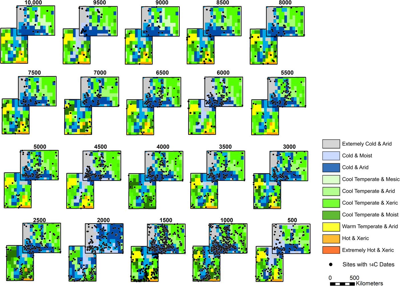
FIGURE 1. Map series of 14C site locations and paleoclimate zones in 500-year intervals, from 10,000 cal BP to 500 cal BP.
While others discuss the validity and reliability of the modeled global climate model inputs (Hargreaves Reference Hargreaves2010; Hargreaves et al. Reference Hargreaves, Annan, Ohgaito, Paul and Abe-Ouchi2013; Kohfeld and Harrison Reference Kohfield and Harrison2000; Nikolova et al. Reference Nikolova, Yin, Berger, Singh and Karami2013; van den Hurk et al. Reference van den Hurk, Braconnot, Eyring, Friedlingstein, Glecker, Knutti, Teixeira, Asrar and Hurrell2013), it is not possible to statistically verify the shape of the modeled paleoclimate zones presented here because many past ecological communities lack modern analogs to make equivalent climate comparisons (the so-called no-analog climates; Gonzales et al. Reference Gonzales, Williams and Grimm2009; Jackson and Overpeck Reference Jackson and Overpeck2000; Veloz et al. Reference Veloz, Williams, Blois, He, Otto-Bliesner and Liu2012; Williams and Jackson Reference Williams and Jackson2007; Williams and Shuman Reference Williams and Shuman2008). These no-analog climates make correlating fossil pollen data to the paleoclimate zones modeled here unfeasible because the climate envelopes for many of the plant taxa used to reconstruct past climates are elastic. This elasticity is evidenced specifically by intraspecies adaptation to local environments, atmospheric levels of CO2, and the potential evolution/adaptation of a species to new environments based on continental- to local-scale climatic changes (Veloz et al. Reference Veloz, Williams, Blois, He, Otto-Bliesner and Liu2012; Williams and Jackson Reference Williams and Jackson2007). Thus, the 15 paleoclimate zones delineated and classified in this study are mathematical estimates of real-world, abiotic processes and should be viewed as our current best estimate of the climate landscape during the Holocene.
Developing Radiocarbon Time Series within Paleoclimate Zones
We develop summed probability distributions (SPDs) of radiocarbon date frequencies from each of the 11 climate zones with dates in Utah and Wyoming, two states where we have large radiocarbon datasets as well as specific site locational data. SPDs are developed from both the precise latitude-longitude or UTM data, and from centroids for each county, for each date. We compare the results obtained for each zone using three spatial resolutions of the radiocarbon data, state, county, and specific levels. As mentioned above, we use county centroids because these are the level of spatial resolution for each date that we submit to CARD and that are effectively coded in sites’ Smithsonian numbers.
A central challenge in working with radiocarbon big data is the variable quality of the individual radiocarbon dates in each state dataset, and we caution researchers against simply downloading and immediately using all dates without implementing some sort of selection criteria. First, despite being called an “archaeological radiocarbon database,” CARD also contains geological and paleontological dates. We must therefore select only archaeological dates. Second, because of the considerable role of variable legacy data in these datasets, some dates do not have associated lab numbers. In order to conduct work within an Open Science approach that provides the means for testing and replicating results, any analysis must have a lab number for each date used. Third, only normalized dates should be calibrated and summed, which requires us to omit all measured dates (or accept these as normalized dates with an assumed δ13C value). Fourth, the older legacy dates have errors anywhere from 300 to 1,000 years. In this analysis, we only include dates with errors <200 years. Lastly, in order to correct for sampling biases caused by oversampling at a particular site, we use only dates with associated site IDs. Using these criteria alongside the requirement that each date have a georeference, Utah's dataset decreased from 3,363 to 1,126 dates, and Wyoming's decreased from 5,830 to 2,570 dates.
The first step in our method requires that we embed each georeferenced date into one of the 11 designated climate zones. Because these different zones are broken down in 500-year intervals, we start by calculating the median calibrated age for each individual radiocarbon date. We do this in OxCal version 4.2 (Bronk Ramsey Reference Bronk Ramsey2009) using the IntCal13 calibration curve (Reimer et al. Reference Reimer, Bard, Bayliss, Warren Beck, Blackwell, Ramsey, Buck, Cheng, Lawrence Edwards, Friedrich, Grootes, Guilderson, Haflidason, Hajdas, Hatté, Heaton, Hoffmann, Hogg, Hughen, Felix Kaiser, Kromer, Manning, Niu, Reimer, Richards, Marian Scott, Southon, Staff, Turney and van der Plicht2013). These median dates place each radiocarbon date into a specific climate zone for each 500-year interval. All dates for each climate zone are then exported from the GIS in order to create an SPD for each zone.
We develop two sets of SPDs using the rcarbon package (Bevan et al. Reference Bevan, Crema and Silva2017) in the R statistical computing language (R Core Team 2014), one using precise site locational data and the other using county centroid data. Rcarbon enables the calibration of dates, the binning of calibrated dates from the same site, the aggregation of dates and development of SPDs, Monte Carlo simulations providing tests for significant positive or negative deviations of the SPD from a selected null model, and permutation tests to compare different regions to each other. As our sample sizes for each climate zone vary, Monte Carlo simulations are important for determining spurious peaks or troughs in the SPDs versus truly significant deviations from the null model. Despite these varying sample sizes, Timpson and colleagues (Reference Timpson, Colledge, Crema, Edinborough, Kerig, Manning, Thomas and Shennan2014) have shown the robustness of the rcarbon method even with small sample sizes.
Our analysis calibrated dates using the IntCal13 calibration curve (Reimer et al. Reference Reimer, Bard, Bayliss, Warren Beck, Blackwell, Ramsey, Buck, Cheng, Lawrence Edwards, Friedrich, Grootes, Guilderson, Haflidason, Hajdas, Hatté, Heaton, Hoffmann, Hogg, Hughen, Felix Kaiser, Kromer, Manning, Niu, Reimer, Richards, Marian Scott, Southon, Staff, Turney and van der Plicht2013). We used the binning function of rcarbon to aggregate multiple dates from the same site that are within 100 calibrated years of each other. SPDs were developed with a 100-year running mean. We carried out 500 Monte Carlo simulations comparing the empirical SPDs against a null model of exponential growth. We did not correct for taphonomic bias for two reasons. First, the exponential null model assumes the same increasing loss of radiocarbon samples through time (Crema et al. Reference Crema, Habu, Kobayashi and Madella2016). Second, taphonomic correction (Bluhm and Surovell Reference Bluhm and Surovell2018; Surovell et al. Reference Surovell, Finley, Smith, Jeffrey Brantingham and Kelly2009) does not alter the amount of significant positive or negative deviations from the null model compared to non-taphonomically corrected SPDs; it just increases the frequencies of radiocarbon dates for all SPDs in the middle Holocene relative to the late Holocene.
RESULTS: PALEODEMOGRAPHY AND PALEOCLIMATE
As noted above, this paper proposes a new method for reconstructing human paleodemography from radiocarbon SPDs. This method moves beyond traditional approaches that develop SPDs for arbitrarily defined geographic regions. We propose developing SPDs from transient climate models that can provide more realistic assessments of the geographic and environmental spaces inhabited by prehistoric human populations. This method requires high-quality spatial data, which we will critically assess here.
State-Wide SPDs Versus Climate Zone SPDs
Figure 2 shows the Holocene SPDs for the entire states of Utah and Wyoming. Figure 3 shows the SPDs for the different climate zones using precise site locational data for each radiocarbon date. Figure 4 compares the significant population “booms” and “busts” from SPDs at the state-wide level to the different climate zones.
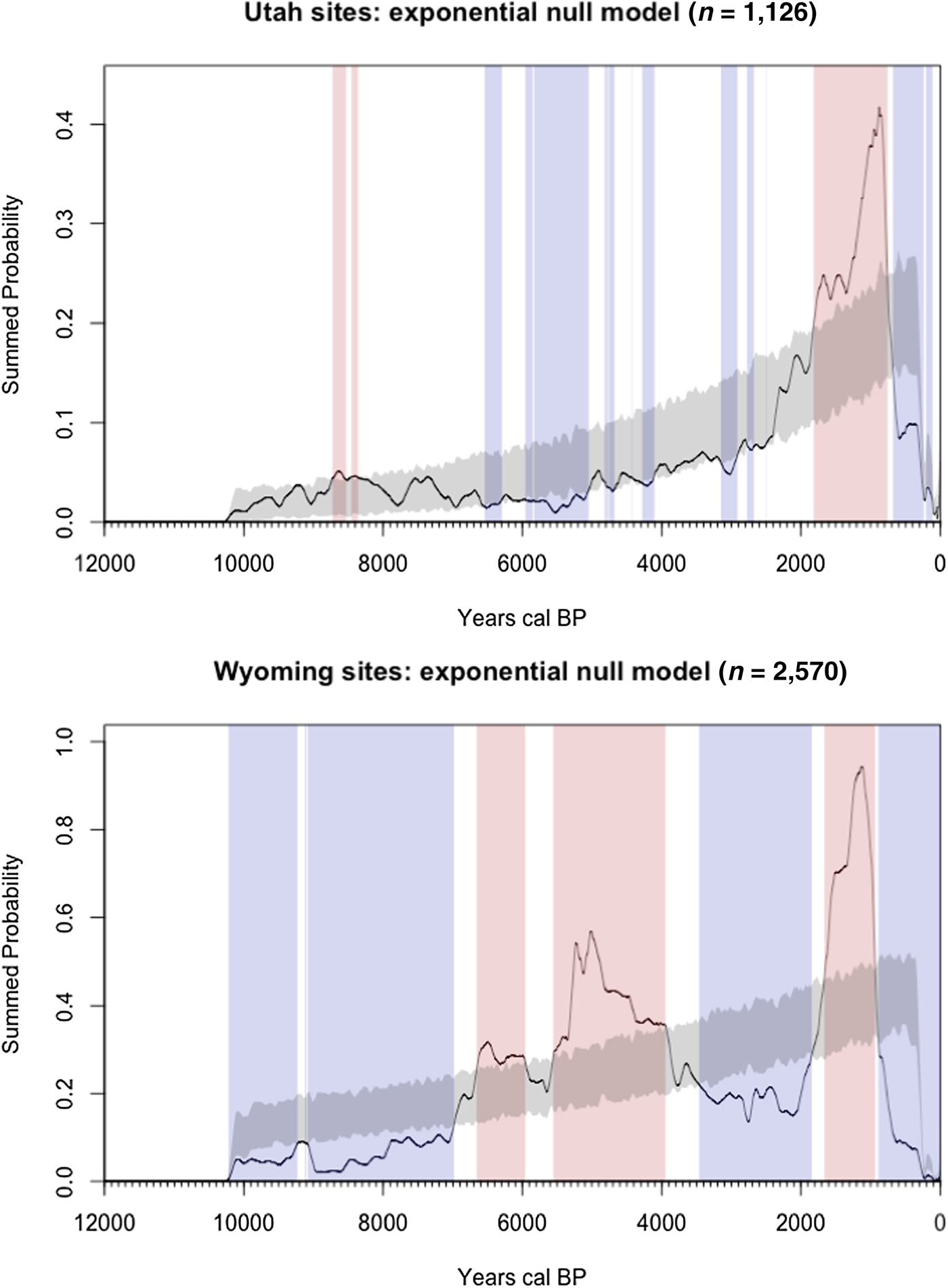
FIGURE 2. Radiocarbon Summed Probability Distributions (SPD) for Utah and Wyoming. Black line: empirical SPD with 100-year running mean. Gray band: exponential null model with 95% confidence limits. Blue: significant negative deviations from the null model (i.e., population “busts”). Red: significant positive deviations from the null model (i.e., population “booms”).
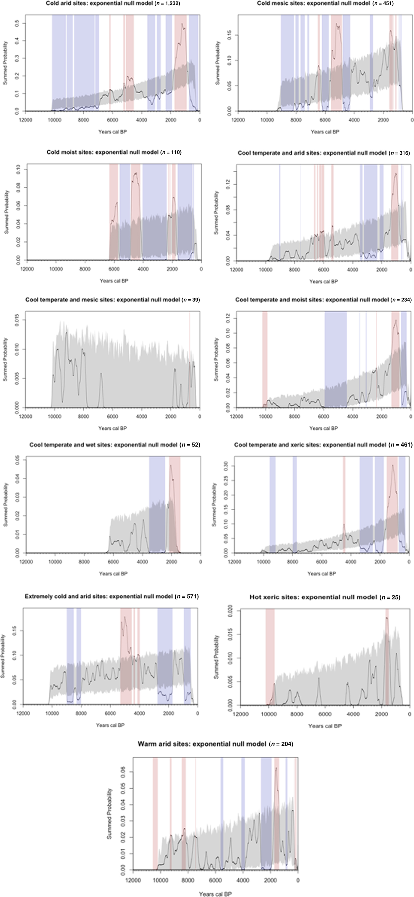
FIGURE 3. Radiocarbon Summed Probability Distributions (SPD) for climate zones with precise site locational data. Black line: empirical SPD with 100-year running mean. Gray band: exponential null model with 95% confidence limits. Blue: significant negative deviations from the null model (i.e., population “busts”). Red: significant positive deviations from the null model (i.e., population “booms”).

FIGURE 4. Comparison of significant population “booms” and “busts” between states and among climate zones with precise site locational data. Black: population “busts.” Gray: population “booms.” White: no significant deviation from the exponential null model.
Figure 4 displays the unique power of the “dates as data” approach to provide coarse-grained reconstructions of human paleodemography. At the state-wide level, some interesting patterns are immediately apparent. First, we see that during the early Holocene, Wyoming exhibits significant population busts, while Utah shows a slight boom within a broader period that fits within the expected trends of the exponential null model. The opposite occurred during the middle Holocene, when we see a population boom in Wyoming at the same time that a population bust appears in Utah. At this coarse-grained scale, these patterns suggest possible population migration. We reiterate that the coarse-grained nature of SPDs provides first approximations, enabling the development of testable hypotheses (Williams Reference Williams2012). These state-wide comparisons suggest that future research explore and test hypotheses for the migration of populations out of the eastern Great Basin during the middle Holocene.
However, when we compare state-wide trends to the different climate zones, the hypothesis for human migration becomes more complex. Significant population booms or busts are not recorded for each climate zone during the early and middle Holocene. This suggests more complex and nuanced vulnerabilities to booms or busts for different environmental contexts.
The different climate zone SPDs suggest that certain zones might have been more susceptible to demographic fluctuations than others. This enables us to ask questions that align with central questions in population ecology, such as the processes by which species inhabit and fill in different landscapes (Allee et al. Reference Allee, Park, Emerson, Park and Schmidt1949; Berryman Reference Berryman1999; Fretwell and Lucas Reference Fretwell and Lucas1969). The ability to ask questions that align with population ecology is a key benefit of climate zone approaches to SPDs. The climate zones in Figure 4 enable us to have a coarse-grained perspective on how prehistoric human populations filled in different ecosystems throughout Utah and Wyoming during the Holocene. The patterns of different booms, busts, and expected populations between the different climate zones highlight how, during the early and middle Holocene, human populations were able to adapt to environmental or social perturbations by simply moving from one environmental context to another. This ability to migrate is apparent by the mix of booms, busts, and expected population levels for the different time slices during the early and middle Holocene. The late Holocene highlights a very different situation, in which we see a greater number of contemporaneous booms or busts across all climate zones. The large number of population busts across most climate zones ~3000 cal BP suggests something like the beginning of a broad-scale population turnover, with populations starting to grow ~2000 cal BP, populations booming from ~2000–1000 cal BP, and populations busting after ~1000 cal BP. At this coarse-grained scale, it appears that the relatively contemporaneous boom and bust pattern across different environmental contexts shows that human populations were saturating landscapes throughout Utah and Wyoming during the late Holocene. Whereas early and middle Holocene populations were able to move freely among different environmental contexts because they were sparsely populated, late Holocene populations had to contend with landscapes that were fully populated—which, we propose, initiated new population ecology processes guided more by endogenous social-ecological, and perhaps epidemiological (e.g., Phillips et al. Reference Phillips, Wearing and Clark2018), processes. This might be attributed to both the impact of the spread of domesticated plants into certain zones (Simms Reference Simms2008) and large-scale migration into the region (e.g., Madsen and Simms Reference Madsen and Simms1998; Thomas Reference Thomas2019). This widespread population boom-bust ~1000–700 cal BP is the subject of ongoing research, as it appears to have occurred across many regions throughout North America and even the world (Chaput and Gajewski Reference Chaput and Gajewski2016; Freeman et al. Reference Freeman, Baggio, Robinson, Byers, Gayo, Finley, Meyer, Kelly and Anderies2018; Peros et al. Reference Peros, Munoz, Gajewski and Viau2010).
Although it is not our aim in this article to further elaborate on these initial interpretations, our comparison of state-wide and climate zone SPDs indicate that climate-zone SPDs provide an exciting foundation for asking fundamental questions about human population ecology. The coarse-grained scales offered by climate-zone SPDs also enable new perspectives on some of the most dominant research themes in the archaeology of the western United States, such as the Numic Spread hypothesis, the spread of maize agriculture beyond the Southwest, and the widespread late prehistoric collapse of populations across different social-ecological contexts throughout the West.
Precise Site Location SPDs versus County Centroid SPDs
As we are currently releasing data that we have collected from our NSF project to CARD in the form of county centroids, we seek to compare results of climate-zone SPDs using county centroid versus those using precise site locational data. We developed SPDs for county centroid climate zones using the same parameters we used for the SPDs with site locational data. Figure 5 shows these different SPDs. Figure 6 compares the booms and busts for the different climate zones using centroid versus site location data.
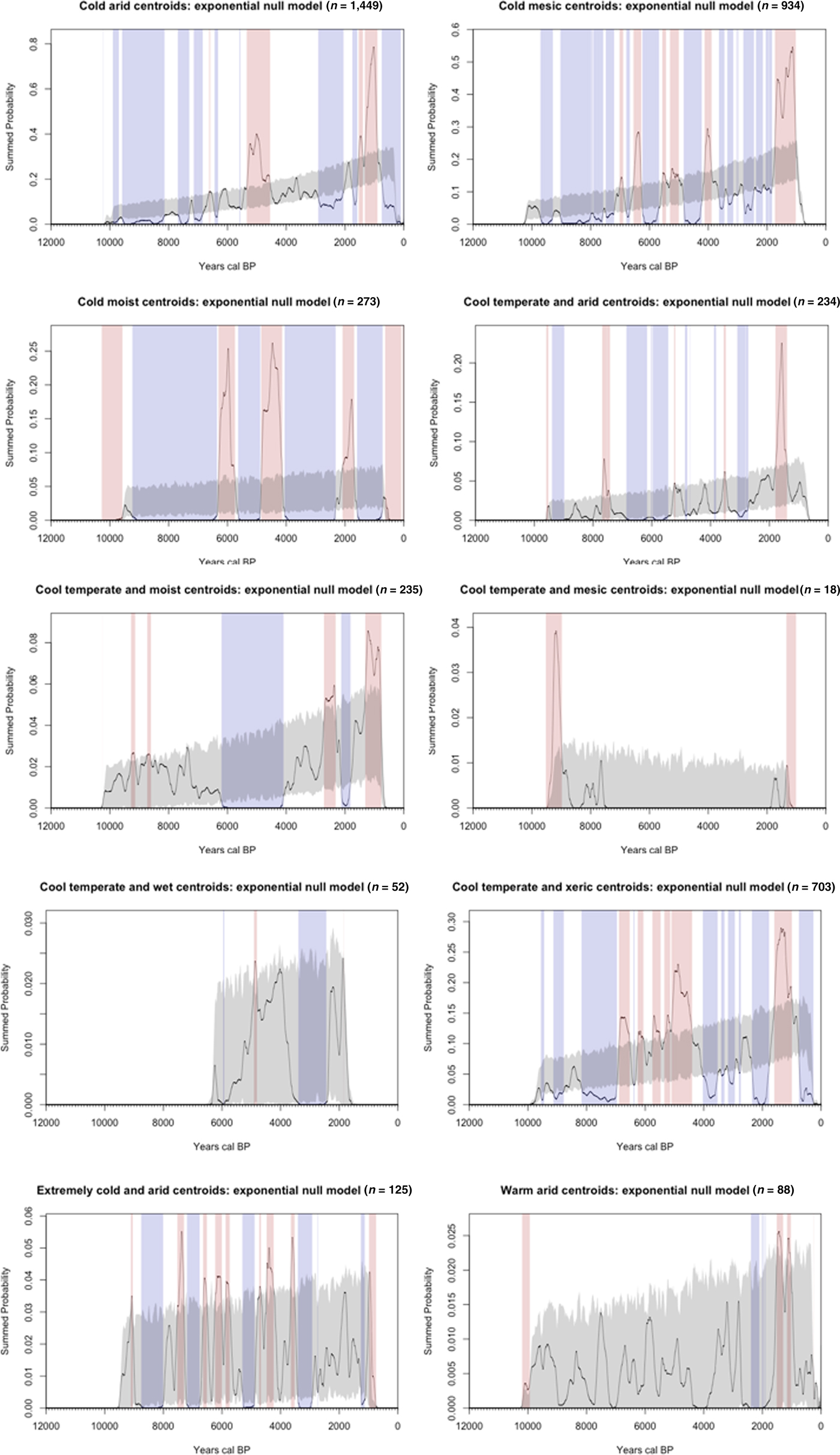
FIGURE 5. Radiocarbon Summed Probability Distributions (SPD) for climate zones with county centroid data. Black line: empirical SPD with 100-year running mean. Gray band: exponential null model. Blue: significant negative deviations from the null model (i.e., population “busts”). Red: significant positive deviations from the null model (i.e., population “booms”).

FIGURE 6. Comparison of significant population “booms” and “busts” between different climate zones for county centroid and site locational data. Black: population “busts.” Gray: population “booms.” White: no significant deviations from the exponential null model.
The assignment of the spatial location of each radiocarbon date to a specific climate zone for a 500-year interval shows significant mismatches between the county centroid data and site locational data for each state (Wyoming χ 2 = 963, df = 19 p < 0.000; Utah χ 2 = 176, df = 19 p < 0.000). Table 1 shows the number of total mismatching dates assigned to climate zones for each 500-year interval for Utah. In total, there is a significant mismatch for Utah, where 53% of the radiocarbon dates using centroid data were assigned to the wrong climate zones than with precise site locational data. Table 1 also shows the number of total mismatching climate zones for Wyoming. In total, there is a significant mismatch for Wyoming, where 77% of the radiocarbon dates using centroid data were assigned to the wrong climate zones than when using precise site locational data.
TABLE 1. Comparing Mismatching Climate Zones between Precise Site Location Data and County Centroid Data for Utah and Wyoming.

CONCLUSION
Given the size of most counties in western states, it is no surprise that low-resolution county centroid data causes the misassignment of dates to particular climate zones. The point is that such data cause major problems for using open-access radiocarbon dates for research on human paleodemography and human-environment interaction throughout prehistory. As Figure 6 illustrates, the county centroid data show more booms and busts than the precise site locational data. This could lead to overinterpretations of prehistoric human population dynamics, with the different climate zones seeming more vulnerable to boom-bust dynamics. As SPDs are coarse-grained, first approximations of prehistoric demography, we must minimize overinterpretations such as these. Furthermore, for certain periods of time in certain climate zones, county centroid data show busts when the site locational data show booms. The precise site locational data provide not only more realistic and accurate reconstructions of human demography in paleoclimate space but also more conservative assessments of the data, which can minimize the potential for misinterpretation or overinterpretation of these coarse-grained population trajectories.
We have made the case here for the use of locational data that is as precise as possible. And this is as important to research as it is to CRM, which needs access to spatial data to plan for development and land management. Obviously, there is really no argument that precise data are more useful than imprecise data. The problem comes in accessing those data. A researcher has the option to seek site locations from the relevant state authorities. But if one's research question requires multiple states, or the entire country, that researcher will encounter a considerable amount of additional work and may be denied access, leaving a gap in data and forcing a less precise analysis.
So, what to do? How do we protect sites and yet make spatial data available to researchers with minimal effort? We note that the SAA has recently created a Task Force of Sharing Public Outcomes of CRM, chaired by Joshua Wells (Indiana University, South Bend), whose mandate includes drafting guidelines for the sharing of site location for research purposes. We look forward to the task force's report and offer three suggestions.
First, this issue requires a conversation with relevant federal agencies, beginning with the lead agency on archaeological matters: the National Park Service. All parties, including federal and state entities, must recognize that we no longer operate in the research environment that existed when protective legislation was enacted in the 1960s and 1970s. A regional study in the 1970s was probably contained within a state, but one today might encompass the continent (or even the world; see Freeman et al. Reference Freeman, Baggio, Robinson, Byers, Gayo, Finley, Meyer, Kelly and Anderies2018). The idea of Big Data didn't exist in the 1960s and 1970s, nor did the technology to store and analyze large datasets that crosscut state boundaries. This has now changed. By controlling access to data, state authorities, as well as the federal authorities that provide legislative guidance, must recognize their ethical responsibility to assist in this new research paradigm. This includes the recognition that tribal sovereignty and consultation are central to developing new guidelines for data sharing in the twenty-first century.
Second, state authorities could require that database gatekeepers (such as CARD) explicitly accept responsibility for the misuse of information contained in their databases. This might take the form of language in, for example, memoranda of understanding (MOUs) that absolve state authorities from responsibility should data given to databases be misused. Additionally, and accordingly, gatekeepers should create rigorous vetting procedures and publish them. These could include notification of the relevant state authorities when a state's data are downloaded.
Third, locational data in databases could be made intentionally imprecise at a scale that protects site location and yet allows researchers to proceed with most spatial analyses. For example, site location could be masked by taking a site's actual location, choosing a random direction (0 to 359 degrees), and then choosing a random distance (e.g., between 2 and 5 km). That might be enough to ensure that unauthorized personal could not find the actual site (the published location would always be, in this example, at least 2 km away in an unknown direction) but not so far off that it would impede spatial analyses. Such an approach would also alert analysts to the maximum level of error in spatial data and allow them to decide whether it is acceptable for their research.
The era of Big Data is upon us. It requires that we rethink how we approach the control and dissemination of information, and that means an open dialogue concerning the quality of open-source spatial data. If not, our discipline will miss a unique opportunity to make important contributions to the public that funds our work. And if we cannot learn from prehistory, then that hands ammunition to those who would seek to recall protective legislation. The future preservation of the archaeological record goes hand-in-hand with its ability to be used by researchers and accessed by all stakeholders (Clarke Reference Clarke2015; Faniel et al. Reference Faniel, Austin, Kansa, Kansa, France, Jacobs, Boytner and Yakel2015; Huggett Reference Huggett2015; Kansa Reference Kansa2012).
Acknowledgments
Funding for this research was provided by NSF grants 14-18858, 16-24061, and 18-22033 (to RLK). We thank Brian Codding for helping collect Utah data. We thank Sarah Allaun for translating the abstract into Spanish. Permits were not required for this research.
Data Availability Statement
No original data were presented in this article.


