


NOMENCLATURE
- A e
set of all outgoing edges from j (for e = (i, j)) that form an angle ≤ α with e
- a s
area of sector s
- ATCO
air Traffic Controller
- ATM
air Traffic Management
- b i,j
signed area of a triangle formed by edge (i, j) and reference point r
 \[
{\cal C}
\]
\[
{\cal C}
\]set of constraints on the resulting sectors
- Eurocontrol
european Organisation for the Safety of Air Navigation
- \[
{\cal E}{\cal P}
\]
set of (snapped) entry points
- \[
{\cal F}
\]
objective function
- FAA
federal Aviation Administration of the United States
- f e
flow variable that gives the flow on edge e = (i, j), that is, the flow from i to j
- G
graph for route construction
- G 2
grid graph for sectorisation
- \[
{\cal H}
\]
set of hotspots
- h i,j
signed heat value of a triangle formed by edge (i, j) and reference point r
- h q
heat value for each discrete heatmap point q
- L
lower bound that ensures merge point separation
- l i,j
length of edge (i, j)
- MIP
mixed Integer Programming
- \[
q_{j,m}^s
\]
indicates whether at j a chain with counterclockwise (clockwise) triangles switches to a chain of clockwise (counterclockwise) triangles
- \[
qabs_{j,m}^s
\]
- \[
|q_{j,m}^s |
\]
- P
simple polygon
- p i,j
sign of b i,j
- p i,j,m
sign of a triangle formed by edge (i, j) and reference point r m
- phy i,j,s
h i,j · y i,j,s
- R
runway
- RF
radius Arc to a Fix
- RWY
runway
- r, r 1, ..., r 4
reference points
- S i
sectors
- S 0
artificial sector that encompasses the complete boundary of P, using all counterclockwise edges
- SESAR
single European Sky ATM Research
- SID
standard Instrument Departure
- STAR
standard Terminal Arrival Route
- t s
taskload of sector s
- TMA
terminal Maneuvering Area
- \[
{\cal V}(p)
\]
voronoi cell for a given site p
- Vor(S)
voronoi diagram for a set of sites S
- w i,j
edge weight that depends on the heat-values of the edge’s endpoints
- x e
decision variable that indicates whether edge e ∈ E particiaptes in the STAR
- y i,j,s
decision variable that indicates whether edge (i, j) is boundary edge for sector s
- \[
z_{i,j,m}^s
\]
- \[
qabs_{j,m}^s \cdot y_{i,j,s}
\]


Greek symbols
- α e
|A e|
- δ(i)
degree of vertex i in the underlying graph of the chosen STAR edges
- ϰ i
number of aircraft that enter the TMA via
\[
i \in {\cal E}{\cal P}
\]- ω η
weight for each hotspot
\[
\eta \in {\cal H}
\]


1.0 INTRODUCTION
In general, terminal airspace design involves bringing functionality to all three air traffic management (ATM) systems—airspace management (design of arrival and departure route configurations), air traffic flow and capacity management (mapping aircraft to available capacity) and air traffic control (in particular, splitting the airspace into sectors). A plethora of work—from basic research to proof-of-concept validations to large-scale simulations to real-world tests to commercial implementations—has been done on each of the three systems.
Previously, trajectory planning and sectorisation were considered separately, as two different problems. This was partially due to intractability of the combined problem with earlier computational tools and partially to historical reasons (the need for trajectory optimisation arose in some instances, while sector redesign was called for at other places/times).
At the same time, EUROCONTROL’s and FAA’s innovative vision (promoted, in particular in SESAR and NextGen initiatives via the Flexible Use of Airspace paradigm) puts traffic flow and capacity management into the heart of ATM, making both airspace management and design for control derivatives of a single encompassing optimisation task. Thus, in this paper we develop two unified approaches to airspace design by simultaneously delivering flight paths and sectors configurations.
Our mixed integer programming (MIP)-based approach combines two of our prior grid-based MIP formulations for Terminal Maneuvering Area (TMA) sectorisation and for the design of arrival routes. We show how we can combine these two approaches to a single MIP, and that we can integrate constraints on the interaction between sector boundary and arrival routes. That is, we create a single MIP that simultaneously optimises the arrival routes and the sectorisation.
Our second, Voronoi-based, approach is based on using disjoint disks to separate potential “hotspots” of air traffic controller (ATCO) activity on the terminal routes. The disks must stay disjoint both between themselves and from the sector boundaries; the boundaries can be moved, giving the airspace designer the freedom of re-sectorisation.
One of our main technical novelties is the suggestion to abandon the trajectories-to-complexity-to-sectors scheme (the golden standard for sectorisation solutions) and instead directly build sectors around the potential conflicts on the routes themselves (eliminating the construction of the complexity map). We also suggest that different parts of sector boundaries may be constrained with different “strength” – some parts must be subject to hard constraints, while the rest of the boundaries may be treated as “soft” connections; this adheres to the generic paradigm of “providing structure where necessary and flexibility where possible”.
We define our approaches for 2D and run our experiments in 2D. However, the general concepts transfer to 3D, though, the MIP-based approach will be computationally intensive (and potentially computationally infeasible).
We apply our model to the TMA, as Standard Terminal Arrival Routes (STARs) and Standard Instrument Departures (SIDs) quite clearly define the traffic layout.
1.1 Related work
Large body of prior and ongoing ATM research is devoted to both route planning and to sectorisation; here we cite only few papers that addressed the problems.
Many path and flow planning algorithms take into account sectors and their capacities, specified as a part of the input to the algorithm. The classical examples are papers by Bertsimas and Stock Patterson(Reference Bertsimas and Patterson2) and by Lulli and Odoni(Reference Lulli and Odoni17). In its turn, capacity estimation for weather-impacted airspace has been done while treating sector boundaries as obstacles impenetrable by the routed paths(Reference Krozel, Mitchell, Polishchuk and Prete15,Reference Krozel, Mitchell, Polishchuk and Prete16) .
Sectorisation, on the other hand, takes trajectories as the input, builds the complexity map (using, e.g. the Dynamic Density(Reference Kopardekar, Schwartz, Magyarits and Rhodes14) or other approaches(Reference Zohrevandi, Polishchuk, Lundberg, Svensson, Johansson and Josefsson26)) and then splits the airspace into sectors balancing the complexity. The sectorisation algorithms range from synthesising the sectors out of elementary cells (hexagons(Reference Yousefi23), square pixels(Reference Brinton, Leiden and Hinkey3), 3D voxels(Reference Jägare, Flener and Pearson13), and others(Reference Sergeeva, Delahaye, Mancel, Zerrouki and Schede22)) via mathematical programming, to graph-based approaches(Reference Delahaye, Schoenauer and Alliot4) in which sector boundaries are Voronoi diagram edges (or faces, in 3D)(Reference Gerdes, Temme and Schultz9), to using computational-geometry techniques to partition the airspace (e.g. binary space partitions(Reference Basu, Mitchell and Sabhnani1)); see the surveys(Reference Flener and Pearson8,Reference Prandini, Piroddi, Puechmorel and Brázdilová20) for a comprehensive overview.
To our knowledge no prior work considered designing both routes and sectors within a single framework (the notable exception is(Reference Pfeil19) Section 5, where a very simplified, but dynamic, model was considered, in which both STARs/SIDs and sectors boundaries were radial segments going from the airport to the TMA boundary). In practice, it may be necessary to go through the design of sectors and routes one by one, iteratively adjusting ones while keeping the others fixed, as suggested, e.g. by the Manual for airspace planning from Eurocontrol(6).
Even though no prior work is a direct predecessor of this paper, we borrow many ideas from previous research. Our hotspot definition is inspired by the work of Netjasov et al.(Reference Netjasov, Janić and Tošić18). The requirement that the routes change sectors (nearly) perpendicularly to the boundary between the sectors appears in(Reference Sabhnani, Yousefi and Mitchell21).
1.2 Roadmap
In Section 2 we present notation used in the rest of the paper. In Section 3 we review our MIP-formulations for arrival routes and sectorisation from prior work, as these build the basis for the combined MIP. In Section 4 we explain how we deduce hotspots from any route layout. We present the combined MIP-based approach in Section 5. Our second, Voronoi-based, approach is described in Section 6. We apply both approaches to Stockholm TMA in an experimental study in Section 7, before we conclude the paper in Section 8.
2.0 NOTATION AND PRELIMINARIES
A simple polygon P is given by a set of n vertices υ 1, υ 2, ..., υ n and n edges υ 1υ 2, υ 2υ 3, ..., υ n−1υ n, υ nυ 1 such that no pair of non-consecutive edges share a point. P is the closed finite region bounded by the vertices and edges. A sectorisation of a simple polygon P is a partition of the polygon P into k disjoint subpolygons S 1 ... S k (S i ∩ S j = ∅ ∀i ≠ j), such that  \[
\cup _{i{\kern 1pt} = {\kern 1pt} 1}^k S_i = P
\]. The subpolygons S i are called sectors.
\[
\cup _{i{\kern 1pt} = {\kern 1pt} 1}^k S_i = P
\]. The subpolygons S i are called sectors.
Sectorisation Problem:
Given: The coordinates of the TMA, defining a polygon P, the number of sectors  \[
|{\cal S}|
\], a set
\[
|{\cal S}|
\], a set  \[
{\cal C}
\] of constraints on the resulting sectors, and possibly an objective function
\[
{\cal C}
\] of constraints on the resulting sectors, and possibly an objective function  \[
{\cal F}
\].
\[
{\cal F}
\].
Find: A sectorisation of P with  \[
k = |{\cal S}|
\], fulfilling all constraints in
\[
k = |{\cal S}|
\], fulfilling all constraints in  \[
{\cal C}
\], and possibly optimising
\[
{\cal C}
\], and possibly optimising  \[
{\cal F}
\].
\[
{\cal F}
\].
Standard Terminal Arrival Route Problem:
Given: The coordinates of the entry points and the runway, a set  \[
{\cal C}'
\] of constraints on the resulting routes, and possibly an objective function
\[
{\cal C}'
\] of constraints on the resulting routes, and possibly an objective function  \[
{\cal F}''
\].
\[
{\cal F}''
\].
Find: A tree with entries as leaves and runway as the root, fulfilling all constraints in  \[
{\cal C}'
\], and possibly optimising
\[
{\cal C}'
\], and possibly optimising  \[
{\cal F}''
\].
\[
{\cal F}''
\].
Combined Sectorisation and Routes Problem:
Given: The coordinates of the TMA, defining a polygon P, the number of sectors  \[
|{\cal S}|
\], a set
\[
|{\cal S}|
\], a set  \[
{\cal C}
\] of constraints on the resulting sectors, the coordinates of the entry points and the runway, a set
\[
{\cal C}
\] of constraints on the resulting sectors, the coordinates of the entry points and the runway, a set  \[
{\cal C}'
\] of constraints on the resulting routes, a set of constraints
\[
{\cal C}'
\] of constraints on the resulting routes, a set of constraints  \[
{\cal C}''
\] on the interaction between routes and sectors, and possibly an objective function
\[
{\cal C}''
\] on the interaction between routes and sectors, and possibly an objective function  \[
{\cal F}''
\].
\[
{\cal F}''
\].
Find: A sectorisation of P with  \[
k = |{\cal S}|
\], fulfilling all constraints in
\[
k = |{\cal S}|
\], fulfilling all constraints in  \[
{\cal C}
\], tree with entries as leaves and runway as the root, fulfilling all constraints in
\[
{\cal C}
\], tree with entries as leaves and runway as the root, fulfilling all constraints in  \[
{\cal C}'
\], both fulfilling all constraints in
\[
{\cal C}'
\], both fulfilling all constraints in  \[
{\cal C}''
\]; possibly optimising
\[
{\cal C}''
\]; possibly optimising  \[
{\cal F}''
\].
\[
{\cal F}''
\].
3.0 PRIOR MIPs FOR SECTORISATION AND ROUTES
Before we are able to present our complete MIP, we give a brief summary of our MIPs for routes and sectors, see(Reference Granberg, Polishchuk, Polishchuk and Schmidt10–Reference Granberg, Polishchuk, Polishchuk and Schmidt12) for detailed descriptions.
3.1 Routes
For the routes we solve the Standard Terminal Arrival Route Problem as defined in Section 2: we are given locations of the entry points to the TMA, and the location and direction of the airport runway. In the output we seek an arrival tree (new STARs) that merges traffic from the entries to the runway, i.e. a tree that has the entries as leaves and the runway as the root. Our arrival tree should never merge more than two routes in any point, any two merge points must be separated by a certain distance (we use a parameter L as the threshold), no route along the tree should enforce an aircraft to make a sharp turn, and we require STAR–SID crossings to happen far from the runway to ensure safe separation. We discretised the search space by laying out a square grid in the TMA (and snapping the locations of the entry points and the runway onto the grid). Let  \[
{\cal E}{\cal P}
\] denote the set of (snapped) entry points, and R the runway. The side of the grid pixel is equal to a lower bound L, which ensures merge point separation. Every grid node is connected to its eight neighbours, thus forming a graph G = (V, E). The graph is bi-directed; the only exceptions are the entry points (they do not have incoming edges) and R (it does not have outgoing edges). The length of an edge (i, j) ∈ E is denoted by ℓ ij, and ϰ i aircraft enter the TMA via
\[
{\cal E}{\cal P}
\] denote the set of (snapped) entry points, and R the runway. The side of the grid pixel is equal to a lower bound L, which ensures merge point separation. Every grid node is connected to its eight neighbours, thus forming a graph G = (V, E). The graph is bi-directed; the only exceptions are the entry points (they do not have incoming edges) and R (it does not have outgoing edges). The length of an edge (i, j) ∈ E is denoted by ℓ ij, and ϰ i aircraft enter the TMA via  \[
i \in {\cal E}{\cal P}
\].
\[
i \in {\cal E}{\cal P}
\].
We use decision variables x e that indicate whether the edge e ∈ E participates in the STAR. In addition, we have flow variables: f e gives the flow on edge e = (i, j) (i.e. the flow from i to j).
 $$3\sum\limits_{k:(k,i){\kern 1pt} \in {\kern 1pt} E} f_{ki} - \sum\limits_{j:(i,j){\kern 1pt} \in {\kern 1pt} E} f_{ij} = \left( {\matrix{
{\sum\limits_{k{\kern 1pt} \in {\kern 1pt} {\cal E}{\cal P}} _k \;\;\;\;\;i = R} \cr
{ - _i \;\;\;\;\;i \in {\cal E}{\cal P}} \cr
{0\;\;\;\;\;\;\;\;i \in V\backslash \{ {\cal E}{\cal P} \cup R\} } \cr
} } \right.\;\;$$
$$3\sum\limits_{k:(k,i){\kern 1pt} \in {\kern 1pt} E} f_{ki} - \sum\limits_{j:(i,j){\kern 1pt} \in {\kern 1pt} E} f_{ij} = \left( {\matrix{
{\sum\limits_{k{\kern 1pt} \in {\kern 1pt} {\cal E}{\cal P}} _k \;\;\;\;\;i = R} \cr
{ - _i \;\;\;\;\;i \in {\cal E}{\cal P}} \cr
{0\;\;\;\;\;\;\;\;i \in V\backslash \{ {\cal E}{\cal P} \cup R\} } \cr
} } \right.\;\;$$
 \[x_e \ge \frac{{f_e }}{{{\rm{Σ}}_{κ{\kern 1pt} \in {\kern 1pt} {\cal E}{\cal P}} {\cal ϰ}_κ }}\;\;\forall e \in E
\]
\[x_e \ge \frac{{f_e }}{{{\rm{Σ}}_{κ{\kern 1pt} \in {\kern 1pt} {\cal E}{\cal P}} {\cal ϰ}_κ }}\;\;\forall e \in E
\]
 $$f_e \ge 0\;\;\forall e \in E$$
 $$x_e \in \{ 0,1\} \forall e \in E$$
 $$\sum\limits_{k:(k,i){\kern 1pt} \in {\kern 1pt} E} x_{ki} \le 2\;\;\forall i \in V\backslash \{ {\cal E}{\cal P} \cup R\} $$
 $$\sum\limits_{j:(i,j){\kern 1pt} \in {\kern 1pt} E} x_{ij} \le 1\;\;\forall i \in V\backslash \{ {\cal E}{\cal P} \cup R\} $$
 $$\sum\limits_{k:(k,R){\kern 1pt} \in {\kern 1pt} E} x_{kR} = 1\;\;$$
 $$\sum\limits_{j:(R,j){\kern 1pt} \in {\kern 1pt} E} x_{Rj} \le 0\;\;$$
 $$\sum\limits_{k:(k,i){\kern 1pt} \in {\kern 1pt} E} x_{ki} \le 0\;\;\forall i \in {\cal E}{\cal P}$$
 $$\sum\limits_{j:(i,j){\kern 1pt} \in {\kern 1pt} E} x_{ij} = 1\;\;\forall i \in {\cal E}{\cal P}$$
 $$a_e x_e + \sum\limits_{f{\kern 1pt} \in {\kern 1pt} A_e } x_f \le a_e \;\;\forall e \in E$$
Equation (1) ensures that a flow of  \[
\sum\nolimits_{k \in {\cal E}{\cal P}} _k
\] (of all the aircraft) reaches the runway R, a flow of ϰ i leaves every entry point i, and in all other vertices of the graph the flow is conserved. Equation (2) enforces edges with a positive flow to participate in the STAR. The flow variables are non-negative (Equation (3)), the edge variables are binary (Equation (4)). Constraints (5)–(10) ensure that the outdegree of every node is at most 1 and that the maximum indegree is 2, that is, no more than two routes merge at any point. Equations (7) and (8) ensure that the runway R has one ingoing and no outgoing edges, respectively; Equations (9) and (10) make sure that each entry point has one outgoing and no ingoing edge, respectively; the maximum indegree of 2 for all other vertices is given by Equation (5), the maximum outdegree of 1 by Equation (6). Equation (11) ensures that the turn from a segment of a route to the consecutive segment is never smaller than a given angle threshold α: If an edge e = (i, j) is used, all outgoing edges at j must form an angle of at least α with e. We let A e be the set of all outgoing edges from j that form an angle ≤ α with e, i.e.
\[
\sum\nolimits_{k \in {\cal E}{\cal P}} _k
\] (of all the aircraft) reaches the runway R, a flow of ϰ i leaves every entry point i, and in all other vertices of the graph the flow is conserved. Equation (2) enforces edges with a positive flow to participate in the STAR. The flow variables are non-negative (Equation (3)), the edge variables are binary (Equation (4)). Constraints (5)–(10) ensure that the outdegree of every node is at most 1 and that the maximum indegree is 2, that is, no more than two routes merge at any point. Equations (7) and (8) ensure that the runway R has one ingoing and no outgoing edges, respectively; Equations (9) and (10) make sure that each entry point has one outgoing and no ingoing edge, respectively; the maximum indegree of 2 for all other vertices is given by Equation (5), the maximum outdegree of 1 by Equation (6). Equation (11) ensures that the turn from a segment of a route to the consecutive segment is never smaller than a given angle threshold α: If an edge e = (i, j) is used, all outgoing edges at j must form an angle of at least α with e. We let A e be the set of all outgoing edges from j that form an angle ≤ α with e, i.e.  \[
A_e = \{ (\,j,k):ijk \le \alpha ,(\,j,k) \in E\}
\], and let α e= |A e|, see Fig. 1(a). For the STAR–SID separation, we disallow STAR edges to intersect SID edges within distance d from the runway. That is, we consider the set of all points on SID edges that along the SID have a distance of at most d to the runway, and delete all edges from E that intersect with this set.
\[
A_e = \{ (\,j,k):ijk \le \alpha ,(\,j,k) \in E\}
\], and let α e= |A e|, see Fig. 1(a). For the STAR–SID separation, we disallow STAR edges to intersect SID edges within distance d from the runway. That is, we consider the set of all points on SID edges that along the SID have a distance of at most d to the runway, and delete all edges from E that intersect with this set.
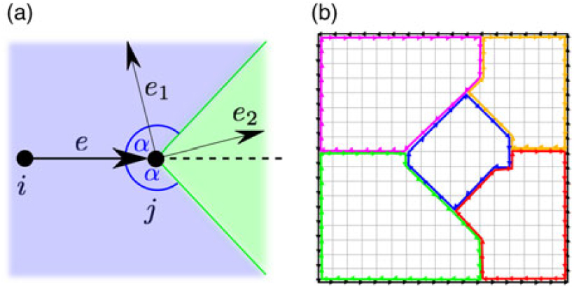
Figure 1. (a) Limited turn: if edge e = (i, j) is used, only edges within the light green region are allowed, that is, edges with an angle of at least α with e. If edges in the light blue region, A e, are used, x e must be set to zero. Here: e 1 ∈ A e, e 2 ∉ A e. (b) Artificial sector S 0 (black) and a sectorisation with  \[
|{\cal S}| = 5
\]. Edges are slightly offset to enhance visibility.
\[
|{\cal S}| = 5
\]. Edges are slightly offset to enhance visibility.
Objective functions. It is natural to seek STARs featuring short flight routes for aircraft. Thus, one objective function in our optimisation problem is the demand-weighted total length of the routes from the entry points to the runway. At the same time, the STAR tree should “occupy little space”—both from the ATCO perspective (to minimise attention attraction area), and to avoid spreading the noise and other environmental impact of aviation over the larger region. This can be modeled by requiring that the produced tree has small total length of the edges. The two objective functions are given in Equations (12) and (13):
 $$3{\rm{[3em][l]min}}\sum\limits_{e{\kern 1pt} \in {\kern 1pt} E} \ell _e f_e $$
 $${\rm{[3em][l]min}}\sum\limits_{e{\kern 1pt} \in {\kern 1pt} E} \ell _e x_e $$
3.2 Sectorisation
We want to solve the sectorisation problem as defined in Section 2. Again, we discretised the search space by laying out a square grid in the TMA. Every grid node has directed edges to its eight neighbours (N(i) = set of neighbours of i (including i)), resulting in a bidirected graph G 2 = (V 2, E 2). The length of an edge (i, j) ∈ E 2 is denoted by ℓ i,j.
The main idea for the sectors is to use an artificial sector, S 0, that encompasses the complete boundary of P, using all counterclockwise (ccw) edges. That is, we use sectors in  \[
{\cal S}^* = {\cal S} \cup S_0
\] with
\[
{\cal S}^* = {\cal S} \cup S_0
\] with  \[
{\cal S} = \{ S_1 \ldots S_k \}
\]. For all edges (i, j) used for boundary of any sector, we enforce that also the opposite edge, ( j, i), is used for another sector, see Fig. 1(b). Thus, all edges of an (interior) sector are clockwise (cw).
\[
{\cal S} = \{ S_1 \ldots S_k \}
\]. For all edges (i, j) used for boundary of any sector, we enforce that also the opposite edge, ( j, i), is used for another sector, see Fig. 1(b). Thus, all edges of an (interior) sector are clockwise (cw).
We use decision variables y i,j,s, where y i,j,s = 1 indicates that edge (i, j) is a boundary edge for sector s. We add the Constraints (14)–(34).
Equation (14) ensures that all ccw boundary edges belong to S 0. Consistency between edges is given by Equation (15): if (i, j) is used for some sector, edge ( j, i) has to be used as well. Equation (16) ensures that a sector cannot contain both edges (i, j) and ( j, i), that is, enclose an area of zero. Together with Equation (15) it ensures that if an edge (i, j) is used for sector S ℓ , the edge ( j, i) has to be used by some sector S x ≠ S ℓ. Equation (17) enforces that one edge cannot participate in two sectors. Equation (18) enforces a minimum size for all sectors. Equation (20) ensures that indegree and outdegree coincide for all nodes. By Equation (21) a node has at most one incoming edge per sector.
 $$3y_{i,j,0} = 1\;\;\forall (i,j) \in S_0 $$
 $$\sum\limits_{s{\kern 1pt} \in {\kern 1pt} {\cal S}^* } y_{i,j,s} - \sum\limits_{s{\kern 1pt} \in {\kern 1pt} {\cal S}^* } y_{j,i,s} = 0\;\;\forall (i,j) \in E_2 $$
 $$y_{i,j,s} + y_{j,i,s} \le 1\;\;\forall (i,j) \in E_2 ,\forall s \in {\cal S}^* $$
 $$\sum\limits_{s{\kern 1pt} \in {\kern 1pt} {\cal S}^* } y_{i,j,s} \le 1\;\;\forall (i,j) \in E_2 $$
 $$\sum\limits_{(i,j){\kern 1pt} \in {\kern 1pt} E_2 } y_{i,j,s} \ge 3\;\;\forall s \in {\cal S}^* $$
 $$y_{i,j,s} \in \{ 0,1\} \;\;\forall (i,j) \in E_2 ,\forall s \in {\cal S}^* $$
 $$\sum\limits_{l{\kern 1pt} \in {\kern 1pt} V_2 :(l,i) \in E_2 } y_{l,i,s} - \sum\limits_{j{\kern 1pt} \in {\kern 1pt} V_2 :(i,j) \in E_2 } y_{i,j,s} = 0\;\;\forall i \in V_2 ,\forall s \in {\cal S}^* $$
 $$\sum\limits_{l{\kern 1pt} \in {\kern 1pt} V_2 :(l,i) \in E_2 } y_{l,i,s} \le 1\;\;\forall i \in V_2 ,\forall s \in {\cal S}^* $$
 $$\sum\limits_{(i,j){\kern 1pt} \in {\kern 1pt} E_2 } b_{i,j} \;y_{i,j,s} - a_s = 0\;\;\forall s \in {\cal S}^* $$
 $$\sum\limits_{s{\kern 1pt} \in {\kern 1pt} {\cal S}} a_s = a_0 $$
 $$a_s \ge a_{LB} \;\;\forall s \in {\cal S}$$
 $$\sum\limits_{(i,j){\kern 1pt} \in {\kern 1pt} E_2 } h_{i,j} \;y_{i,j,s} - t_s = 0\;\;\forall s \in {\cal S}^ $$
 $$t_s \ge t_{LB} \;\;\forall s \in {\cal S}$$
 $$\matrix{
\hfill {3q_{j,m}^s = {1 \over 2}\left( {\sum\limits_{i:(i,j){\kern 1pt} \in {\kern 1pt} E_2 } p_{i,j,m} \;y_{i,j,s} - \sum\limits_{l:(\,j,l){\kern 1pt} \in {\kern 1pt} E_2 } p_{j,l,m} \;y_{j,l,s} } \right)} \cr
\hfill {\forall s \in {\cal S},\;\forall j \in V_2 ,\;\forall m \in {\cal M}} \cr
} $$
$$\matrix{
\hfill {3q_{j,m}^s = {1 \over 2}\left( {\sum\limits_{i:(i,j){\kern 1pt} \in {\kern 1pt} E_2 } p_{i,j,m} \;y_{i,j,s} - \sum\limits_{l:(\,j,l){\kern 1pt} \in {\kern 1pt} E_2 } p_{j,l,m} \;y_{j,l,s} } \right)} \cr
\hfill {\forall s \in {\cal S},\;\forall j \in V_2 ,\;\forall m \in {\cal M}} \cr
} $$
 $$3qabs_{j,m}^s \ge q_{j,m}^s \;\forall s \in {\cal S},\forall j \in V_2 ,\;\forall m \in {\cal M}$$
 $$qabs_{j,m}^s \ge - q_{j,m}^s \;\forall s \in {\cal S},\forall j \in V_2 ,\;\forall m \in {\cal M}$$
 $$3z_{i,j,m}^s \ge 0\;\forall i,j \in V_2 \;\forall s \in {\cal S},\;\forall m \in {\cal M}$$
 $$z_{i,j,m}^s \le qabs_{j,m}^s \;\forall i,j \in V\;\forall s \in {\cal S},\;\forall m \in {\cal M}$$
 $$z_{i,j,m}^s \le y_{i,j,s} \;\forall i,j \in V_2 \;\forall s \in {\cal S},\;\forall m \in {\cal M}$$
 $$3z_{i,j,m}^s \ge \;y_{i,j,s} - 1 + qabs_{j,m}^s \forall i,j \in V_2 \;\forall s \in {\cal S},\;\forall m \in {\cal M}$$
 $$3\sum\limits_{i{\kern 1pt} \in {\kern 1pt} V_2 } \sum\limits_{j{\kern 1pt} \in {\kern 1pt} V_2 } z_{i,j,m}^s = 2\;\forall s \in {\cal S},\;\forall m \in {\cal M}$$
Constraints (14)–(21) guarantee that the union of the  \[
|{\cal S}|
\] pairwise disjoint sectors completely covers the TMA.
\[
|{\cal S}|
\] pairwise disjoint sectors completely covers the TMA.
Constraints (22)–(24) are used to balance the sector size. To do so, we need to assign an area to the sector we selected with the boundary edges. For a polygon P with rational vertices, the area is rational and can be computed efficiently (see Fekete et al.(Reference Fekete, Friedrichs, Hemmer, Papenberg, Schmidt and Troegel7)): we introduce a reference point r, and compute the area of the triangle of each directed edge e of P and r, see Fig. 2(a)/(b). For the complete area of P, we sum up the triangle area for all edges of P: clockwise triangles contribute positive, counterclockwise triangles contribute negative. We denote the signed area of a triangle formed by (i, j) and r as b i,j. Thus, Equation (22) assigns the area of sector s to the variable a s, Equation (23) ensures that the sum of the a s’s equals the area of the complete TMA. We use Equation (24) only if we want to balance the sector size. It gives a lower bound on the size of each sector. This could be a constant, or we use  \[
a_{LB} = c_1 \cdot a_0 /|{\cal S}|
\], with , e.g. c 1 = 0.9.
\[
a_{LB} = c_1 \cdot a_0 /|{\cal S}|
\], with , e.g. c 1 = 0.9.
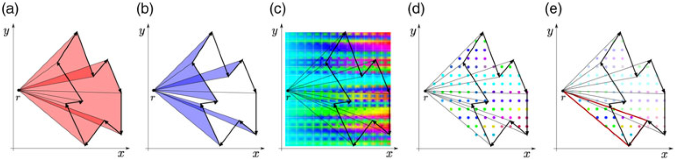
Figure 2. Area of polygon P (bold): each edge of P forms an oriented triangle with a reference point r. Cw triangles contribute positive (a), ccw triangles negative (b). Heat value extraction for a triangle: (c) (Artificial) Heat map overlaid with a grid, (d) heat values extracted at grid points. (e) Shows the discretised heat map for the area of interest for P: the heat values at grid points for all grid points within some triangle of an edge e of P and the reference point r. The highlighted triangle is cw, thus, also its heat value is positive.
The area computation builds the basis for balancing the taskload of all sectors, which we do using Constraints (25)–(26). Here, we assume that a heatmap representing the controller’s taskload is given. Both workload and taskload reflect the demand of the air traffic controller’s monitoring task: the taskload measures the objective demands, while the workload reflects the subjective demand experienced during that task. Recently, Zohrevandi et al.(Reference Zohrevandi24,Reference Zohrevandi, Polishchuk, Lundberg, Svensson, Johansson and Josefsson25) presented a novel model for relating the controller’s taskload to the airspace complexity, represented by eight complexity factors. The authors compared their taskload measure of (weighted) ATCO’s clicks on the radar screen to previous models (Djokic et al.(Reference Djokic, Lorenz and Fricke5)) and were able to explain airspace complexity, given by the eight complexity factors, about 40% better than the model by Djokic et al.; for terminal airspace they achieved an improvement of about 70% (regression analysis factor R 2 = 0.84). Thus, the weighted radar screen clicks are a very good model for terminal airspace complexity. The authors presented heat maps that visualise the density of weighted clicks. We use these heat maps as an input for our sectorisation. Note, that our model does not depend on these specific heat maps, it is a general model that integrates complexity. For the MIP-based computation, we assume that some heatmap representing the controller’s taskload is given, see(Reference Granberg, Polishchuk, Polishchuk and Schmidt11,Reference Granberg, Polishchuk, Polishchuk and Schmidt12) .
Given this heatmap we overlay it with a grid, see Fig. 2(c), extract the value at the grid points, see Fig. 2(d), and use this discretised heatmap, see Fig. 2(e), for further computations. We associate each discrete heatmap point, q, with a “heat value”, h q. Again, we consider triangles for each directed edge (i, j) of P and the reference point r, see, e.g. Fig. 2(e): we sum up the heat values for all grid points within the triangle. The sign of the heat value for a triangle is determined by the sign of b i,j, denoted by p i,j, e.g. the triangle highlighted in Fig. 2(e) is oriented cw (indicated by the red boundary), its heat value is positive (p i,j = +1). Let h i,j denote the signed heat value of the triangle formed by edge (i, j) and r, that is: h i,j = p i,j ∑q ∈ ∆(i,j,r) h q. If the taskload is of interest, we add Equation (25), which assigns each sector s a taskload t s. In analogy to the balanced size, we add Equation (26) to achieve a balanced taskload. We use  \[
a_{LB} = c_1 \cdot a_0 /|{\cal S}|
\] with, e.g. c 2 = 0.9, but t LB could also be chosen as a constant.
\[
a_{LB} = c_1 \cdot a_0 /|{\cal S}|
\] with, e.g. c 2 = 0.9, but t LB could also be chosen as a constant.
With Constraints (27)–(34) we can enforce all sectors to be convex. We can make use of the fact that we have only eight edge directions. For every direction of an incoming edge, there are three directions of outgoing edges that are forbidden in a convex polygon: there exist two open cones in which a reference point must be located to detect the switch. Thus, any reference point located in the intersection of the three cones for all forbidden outgoing edges, yields a switch in the triangle orientation. If we consider all possible edge directions, the cones for the necessary directions overlap. Thus, we only need four points located in the intersection of these cones for all points of the grid: we denote these reference points by r 1, ..., r 4 (r = r m, for some  \[
m \in {\cal M} = \{ 1, \ldots ,4\}
\]). At least one of the r m will result in a cw/ccw switch for non-convex polygons. Let p i,j,m denote the sign of the triangle of the edge (i, j) and reference point r m,
\[
m \in {\cal M} = \{ 1, \ldots ,4\}
\]). At least one of the r m will result in a cw/ccw switch for non-convex polygons. Let p i,j,m denote the sign of the triangle of the edge (i, j) and reference point r m,  \[
m \in {\cal M}
\]. Equation (27) assigns, for each sector, a value of −1,0,1 to each vertex. An interior vertex of either a chain of cw or ccw triangles has
\[
m \in {\cal M}
\]. Equation (27) assigns, for each sector, a value of −1,0,1 to each vertex. An interior vertex of either a chain of cw or ccw triangles has  \[
q_{j,m}^s = 0
\]; if at j a chain with ccw (cw) triangles switches to a chain of cw (ccw) triangles
\[
q_{j,m}^s = 0
\]; if at j a chain with ccw (cw) triangles switches to a chain of cw (ccw) triangles  \[
q_{j,m}^s = - 1\] (\[q_{j,m}^s = 1\]). For a convex sector s, the sum over the
\[
q_{j,m}^s = - 1\] (\[q_{j,m}^s = 1\]). For a convex sector s, the sum over the  \[
|q_{j,m}^s |
\] for all sector vertices j is 2 for all reference points r m; for non-convex sectors this value is larger than 2 for at least one reference point r m. Equations (28) and (29) define the absolute values
\[
|q_{j,m}^s |
\] for all sector vertices j is 2 for all reference points r m; for non-convex sectors this value is larger than 2 for at least one reference point r m. Equations (28) and (29) define the absolute values  \[
qabs_{j,m}^s = |q_{j,m}^s |
\]. To enforce convexity
\[
qabs_{j,m}^s = |q_{j,m}^s |
\]. To enforce convexity  \[
\sum\nolimits_{i \in V_2 } \sum\nolimits_{j \in V_2 } y_{i,j,s} \cdot qabs_{j,m}^s = 2\;\;\forall s \in {\cal S},\;\forall m \in {\cal M}
\] must hold. But, as two variables are multiplied, we cannot add it to the MIP. Instead, we use Equations (30)–(33) to define variables
\[
\sum\nolimits_{i \in V_2 } \sum\nolimits_{j \in V_2 } y_{i,j,s} \cdot qabs_{j,m}^s = 2\;\;\forall s \in {\cal S},\;\forall m \in {\cal M}
\] must hold. But, as two variables are multiplied, we cannot add it to the MIP. Instead, we use Equations (30)–(33) to define variables  \[
z_{i,j,m}^s
\] that take the value of
\[
z_{i,j,m}^s
\] that take the value of  \[
y_{i,j,s} \cdot qabs_{j,m}^s \forall i,j \in V_2 \;\forall s \in {\cal S},\;\forall m \in {\cal M}
\], and add Equation (34).
\[
y_{i,j,s} \cdot qabs_{j,m}^s \forall i,j \in V_2 \;\forall s \in {\cal S},\;\forall m \in {\cal M}
\], and add Equation (34).
3.2.1 Objective function for sectorisation
The objective function for our sectorisation problem is:
 $$3\min \sum\limits_{s \in {\cal S}} \sum\limits_{(i,j){\kern 1pt} \in {\kern 1pt} E_2 } \left( {\gamma \ell _{i,j} + (1 - \gamma )w_{i,j} } \right)y_{i,j,s} ,\;\;0 \le \gamma \le 1$$
Where w i,j represents an edge weight that depends on the heat-values of its endpoints. We choose one of:
(I) w i,j = h i + h j
(II) w i,j = Σk ∈ N(i) h k+ Σl ∈ N(j) h l
For γ = 1: if we want to balance the area of the sectors, but we are not interested in the sector taskload, the objective function ensures that sectors are connected.
If we also take taskload into consideration, the objective function yields connected sectors if our chosen c 2 in  \[
t_{LB} = c_2 \cdot t_0 /|{\cal S}|
\] of constraint (26) allows it: a too high c 2 might not allow a “c 2-balanced” sectorisation with connected sectors. For example, c 2 = 0.95 might ask for too balanced taskloads. But if we allow larger disparities between sectors, we can make a connected solution feasible, e.g. we could lower the parameter to c 2 = 0.6. This is based on the given complexity map: larger imbalances between controller’s taskload must be allowed, if we necessarily need connected sectors.
\[
t_{LB} = c_2 \cdot t_0 /|{\cal S}|
\] of constraint (26) allows it: a too high c 2 might not allow a “c 2-balanced” sectorisation with connected sectors. For example, c 2 = 0.95 might ask for too balanced taskloads. But if we allow larger disparities between sectors, we can make a connected solution feasible, e.g. we could lower the parameter to c 2 = 0.6. This is based on the given complexity map: larger imbalances between controller’s taskload must be allowed, if we necessarily need connected sectors.
For γ < 1, we make sure that points that require increased attention from a controller, that is, points with higher heat values, should lie in the sector’s interior. We call these interior conflict points. (I) ensures that relatively large heat-values are not located on the sector boundary, (II) pushes larger values further into the interior.
4.0 IDENTIFICATION OF HOTSPOTS
Our goal is to present a simultaneous design of routes and sectors. For this approach, we aim to define the potential conflict points, or hotspots, of any route design, which then defines an important part of the interaction between the routes and sectors. That is, based on any SID–STAR combination we aim to identify the hotspots representing the zones of increased attention required from ATCOs. To do so, we presented different SID and STAR combinations to six ATCOs and asked them to identify the hotspots. Based on that, we discussed which type of hotspots any kind of design will induce, that is, we abstracted from the specific given routes to a general route–hotspot relation. The ATCOs identified the runway, entry and exit points with high traffic load, and intersection points of SIDs and STARs as the major hotspots. All of these require close monitoring of ATCOs. We denote the set of resulting hotspots by  \[
{\cal H}
\]. In a second round, we also asked them to rank these hotspots by assigning them a value from low for low attention to high for high attention, these define a weight ω η for each hotspot (on the finest granularity level this is represented by a scale from 1 to 9). For this paper, we will not get into the full details of a 9-value scale, but we will show how different scales can be implemented in our two approaches.
\[
{\cal H}
\]. In a second round, we also asked them to rank these hotspots by assigning them a value from low for low attention to high for high attention, these define a weight ω η for each hotspot (on the finest granularity level this is represented by a scale from 1 to 9). For this paper, we will not get into the full details of a 9-value scale, but we will show how different scales can be implemented in our two approaches.
As a consequence of this process, whenever we compute STARs and SIDs this automatically defines the set of hotspots  \[
{\cal H}
\] and their weights
\[
{\cal H}
\] and their weights  \[
\omega _\eta \forall \eta \in {\cal H}
\].
\[
\omega _\eta \forall \eta \in {\cal H}
\].
5.0 MIP-BASED APPROACH: THE COMBINED MIP
For the combined MIP, we aim to compute routes and sectors simultaneously. That is, we have variables both for selecting arrival route edges (x e and f e) and for selecting sector boundary edges (y i,j,s). We may restrict the way that sector boundary and route edges cross (possibly to achieve close to orthogonal intersections). The graphs of the two grids G and G 2 could be the same, but do not have to be.
Note that our focus is on the computation of STARs and sectors, that is, for a start we keep the current SIDs. The motivation for this is that arriving traffic is slower and thus has more room for maneuverability, while departing traffic leaves the TMA after a well predictable amount of time; in addition, it was confirmed with the practitioners that, e.g. in Stockholm TMA (our guinea pig), current SIDs are satisfactory while the STARs are in need of improvement. On the other hand, the MIP-based approach in general allows to also include the new design of departure routes (with an additional tree construction, using selection variables z e for SID edges, and constraints both on the interaction between STAR and SID edges, and the interaction of SIDs and sector boundaries).
STARs tree vertices of different degrees induce different heat values at their location, which then get split by the sectors. Consequently, our heat values of grid points, h q, are no longer given, but are now variables. Thus, we need to add a set of constraints, which, based on the route edges, defines these heat values h q.
Moreover, we need to adapt Constraint (25). It assigns the heat value of a triangle to the variable t s:
 $$\sum\limits_{(i,j){\kern 1pt} \in {\kern 1pt} E} h_{i,j} \;y_{i,j,s} - t_s = 0\;\;\forall s \in {\cal S}^ $$
Because h q are variables now, so are the signed heat values of the triangles h i,j = p i,j Σq ∈ Δ(i,j,r) h q (note that the p i,j are parameters given for each triangle, the sign of its area). Thus, in Constraint (25) we multiply two variables, which we are not allowed for a linear program. Further we will modify this constraint in accordance to the linear model requirements.
We start with assigning the heat values. We use here the exemplary values assigned according to Fig. 3(c): it assigns heat values to route vertices and their neighbours. In particular, we could use just a subset of these, and only assign a value to high degree vertices. Note that any other assignment by linear constraints would also be possible. We may also set a heat value h q for all or some  \[
q \in {\cal E}{\cal P} \cup \{ R\}
\] that is higher than these values (these do not depend on the location of the routes).
\[
q \in {\cal E}{\cal P} \cup \{ R\}
\] that is higher than these values (these do not depend on the location of the routes).
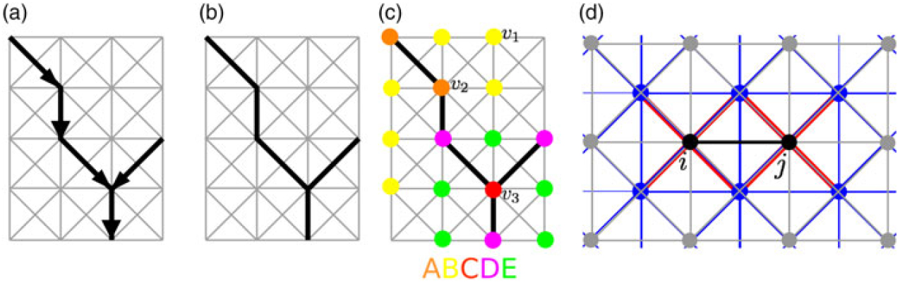
Figure 3. (a) Grid for route edge selection, G, (in gray) with directed SID tree edges (bold black). (b) The underlying undirected graph of the chosen STAR edges. (c) We assign heat values depending on the routes (in the route’s vicinity). Red, pink, green, orange, and yellow gird points get a heat value of C, D, E, A, and B, respectively. (d) G 2 shown in gray, G shown in blue, and a possible set of forbidden route edges for the edge (i, j),  \[
{\cal O}(i,j)
\], shown in red.
\[
{\cal O}(i,j)
\], shown in red.
Let δ(i) = Σk = (k,i) ∈ E x k,i + Σl = (i,l) ∈ E x i,l for all vertices i. That is, δ(i) denotes the degree of the vertex i in the underlying undirected graph of the chosen STAR edges, see Fig. 3(a)/(b). For all vertices we have δ(i) ∈ {0, 2, 3} (except for  \[
\delta (i) \in \{ 0,2,3\}
\]), see for example the routes in Fig. 3(b) where δ(υ 1) = 0, δ(υ 2) = 2, δ(υ 3) = 3. First, we make sure that all heat values are positive, and use Equation (37). For the vertices on the route, we can easily assign the values of at least C for merge points and of at least A for other route vertices. We use Equations (38) and (39), respectively. For the vertices that get assigned the value B: at least one of the neighbours is a route vertex, that is, has degree 2. Using Equation (40) we make sure that the heat value is at least B. A similar idea holds for the neighbours of a merge point: at least one of the neighbours is a route vertex with degree 3, Equation (41) assigns a heat value of at least E accordingly. Finally, we want to assign a value of D to route vertices that are adjacent to a merge point. For any such vertex its own degree is 2, and there is at least one neighbour for which the degree is 3. Consequently, Equation (42) makes sure that these vertices have a heat value of at least D.
\[
\delta (i) \in \{ 0,2,3\}
\]), see for example the routes in Fig. 3(b) where δ(υ 1) = 0, δ(υ 2) = 2, δ(υ 3) = 3. First, we make sure that all heat values are positive, and use Equation (37). For the vertices on the route, we can easily assign the values of at least C for merge points and of at least A for other route vertices. We use Equations (38) and (39), respectively. For the vertices that get assigned the value B: at least one of the neighbours is a route vertex, that is, has degree 2. Using Equation (40) we make sure that the heat value is at least B. A similar idea holds for the neighbours of a merge point: at least one of the neighbours is a route vertex with degree 3, Equation (41) assigns a heat value of at least E accordingly. Finally, we want to assign a value of D to route vertices that are adjacent to a merge point. For any such vertex its own degree is 2, and there is at least one neighbour for which the degree is 3. Consequently, Equation (42) makes sure that these vertices have a heat value of at least D.
 $$3h_q \;\; \ge \;\;0\forall q \in V_2 $$
 $$h_q \ge \;\;C \cdot (\delta (q) - 2)\forall q \in V_2 $$
 $$h_q \ge \;\;A \cdot (\delta (q) - 1)\forall q \in V_2 $$
 $$h_q \ge \;\;B \cdot (\delta (\,j) - 1)\;\;\;\forall q \in V_2 ,\forall j \in N(q)\backslash \{ q\} $$
 $$h_q \ge \;\;E \cdot (\delta (\,j) - 2)\;\;\;\forall q \in V_2 ,\forall j \in N(q)\backslash \{ q\} $$
 $$h_q \ge \;\;D \cdot (\delta (\,j) + \delta (q) - 4)\;\;\;\forall q \in V_2 ,\forall j \in N(q)\backslash \{ q\} $$
We now turn to the adaptation of Constraint (25). Using Equations (43)–(46) we assign the product of h i,j and y i,j,s to the variable phy i,j,s. Let H > |V 2| · max{A, B, C, D, E} and H = −H:
 $$3phy_{i,j,s} \ge \;\;\underline H \cdot y_{i,j,s} \forall i \in V,\forall j \in V,\forall s \in {\cal S}^ $$
 \[
phy_{i,j,s} \;\; \le \;\;H \cdot y_{i,j,s} \forall i \in V,\forall j \in V,\forall s \in {\cal S}*
\]
\[
phy_{i,j,s} \;\; \le \;\;H \cdot y_{i,j,s} \forall i \in V,\forall j \in V,\forall s \in {\cal S}*
\]
 \[
phy_{i,j,s} \ge \;\;h_{i,j} - (1 - y_{i,j,s} ) \cdot H\;\;\forall i \in V,\forall j \in V,\forall s \in {\cal S}^
\]
\[
phy_{i,j,s} \ge \;\;h_{i,j} - (1 - y_{i,j,s} ) \cdot H\;\;\forall i \in V,\forall j \in V,\forall s \in {\cal S}^
\]
 \[
phy_{i,j,s} \le \;\;h_{i,j} - (1 - y_{i,j,s} ) \cdot \underline H \;\;\forall i \in V,\forall j \in V,\forall s \in {\cal S}*
\]
\[
phy_{i,j,s} \le \;\;h_{i,j} - (1 - y_{i,j,s} ) \cdot \underline H \;\;\forall i \in V,\forall j \in V,\forall s \in {\cal S}*
\]
Now we can formulate Constraint (25) as a linear constraint, and add:
 \[
\sum\limits_{(i,j){\kern 1pt} \in {\kern 1pt} E} phy_{i,j,s} - t_s = 0\;\;\forall s \in {\cal S}*
\]
\[
\sum\limits_{(i,j){\kern 1pt} \in {\kern 1pt} E} phy_{i,j,s} - t_s = 0\;\;\forall s \in {\cal S}*
\]
For the intersection constraints, we define, for each edge (i, j) ∈ E 2 a set of forbidden route edges,  \[
{\cal O}(i,j)
\], that is, a set of edges that may not be part of a route in case (i, j) is a sector boundary, see Fig. 3(d) for a possible set
\[
{\cal O}(i,j)
\], that is, a set of edges that may not be part of a route in case (i, j) is a sector boundary, see Fig. 3(d) for a possible set  \[
{\cal O}(i,j)
\]. The set will depend on the two grids defining the graphs G and G 2 and on the distance to the edge (i, j) up to which only an orthogonal route should be allowed. Let
\[
{\cal O}(i,j)
\]. The set will depend on the two grids defining the graphs G and G 2 and on the distance to the edge (i, j) up to which only an orthogonal route should be allowed. Let  \[
o_{i,j} = |{\cal O}(i,j)|
\], note that o i,j is a parameter and not a variable. We add:
\[
o_{i,j} = |{\cal O}(i,j)|
\], note that o i,j is a parameter and not a variable. We add:
 $$\sum\limits_{s{\kern 1pt} \in {\kern 1pt} {\cal S}} (o_{ij} \cdot y_{i,j,s} ) + \sum\limits_{e{\kern 1pt} \in {\kern 1pt} {\cal O}(i,j)} x_e \le o_{i,j} \;\;\forall (i,j) \in E_2 $$
We use all or a subset—depending on which properties we want to ensure, e.g. if we want to have convex sectors—of the Equations (1)–(11), (14)–(24), (26)–(34), (37)–(42), (43)–(47), and (48) for the combined MIP.
5.1 Objective function
As an objective function, we use a convex combination of the objective functions (12), (13), and (35):
 \[
\begin{array}{*{20}c}
{3\min \;\;\beta \left( {\sum\limits_{s{\kern 1pt} \in {\kern 1pt} {\cal S}} \sum\limits_{(i,j){\kern 1pt} \in {\kern 1pt} E_2 } \left( {\gamma \ell _{i,j} + (1 - \gamma )w_{i,j} } \right)y_{i,j,s} } \right)} \hfill \\
{ + (1 - \beta )\left( {\zeta \sum\limits_{e{\kern 1pt} \in {\kern 1pt} E} \ell _e f_e + (1 - \zeta )\sum\limits_{e{\kern 1pt} \in {\kern 1pt} E} \ell _e x_e } \right)} \hfill \\
{\;\;\;\;\;\;0 \le \beta \le 1,0 \le \gamma \le 1,0 \le \zeta \le 1} \hfill \\
\end{array}
\]
\[
\begin{array}{*{20}c}
{3\min \;\;\beta \left( {\sum\limits_{s{\kern 1pt} \in {\kern 1pt} {\cal S}} \sum\limits_{(i,j){\kern 1pt} \in {\kern 1pt} E_2 } \left( {\gamma \ell _{i,j} + (1 - \gamma )w_{i,j} } \right)y_{i,j,s} } \right)} \hfill \\
{ + (1 - \beta )\left( {\zeta \sum\limits_{e{\kern 1pt} \in {\kern 1pt} E} \ell _e f_e + (1 - \zeta )\sum\limits_{e{\kern 1pt} \in {\kern 1pt} E} \ell _e x_e } \right)} \hfill \\
{\;\;\;\;\;\;0 \le \beta \le 1,0 \le \gamma \le 1,0 \le \zeta \le 1} \hfill \\
\end{array}
\]
6.0 VORONOI-BASED APPROACH
While we are able to formulate the simultaneous computation of routes and sectors as a single MIP, actually solving this program is computationally expensive, that is, actually using this MIP to simultaneously compute the routes and sectors is severely limited by the ability to solve this MIP for real-world instances. Thus, we consider a second approach, based on Voronoi diagrams. A Voronoi diagram, for a set of given sites, S, marks the closest site for each point in the plane. That is, the Voronoi diagram partitions the plane into cells, so called Voronoi cells, were the Voronoi cell for a given site p,  \[
{\cal V}(p)
\], is defined as
\[
{\cal V}(p)
\], is defined as  \[
{\cal V}(p) = \{ x \in |\;||x - p|| \le ||x - q||\;\forall \;{\kern 1pt} sites{\kern 1pt} \;q \in S\}
\]. The Voronoi diagram, Vor(S), is the collection of boundaries: points that lie on the boundary of regions that do not have a unique nearest site.
\[
{\cal V}(p) = \{ x \in |\;||x - p|| \le ||x - q||\;\forall \;{\kern 1pt} sites{\kern 1pt} \;q \in S\}
\]. The Voronoi diagram, Vor(S), is the collection of boundaries: points that lie on the boundary of regions that do not have a unique nearest site.
The basic idea for this approach is that a computation of the best possible routes is more important than trying to optimise the sector boundaries: the routes determine how fast and with how much fuel aircraft can reach and leave the runway, and a good design supports controllers to maintain safe separation between aircraft at all times. On the other hand, the sectors should guarantee that points of increased controller interest are not located too close to sector boundaries, to ensure that possible conflicts can be resolved before a handover, and that the taskload for the different controllers is balanced. Thus, it is important that sector boundaries are located as far away as possible from the points of increased controller attention when two of these points need to be separated; the exact location of the remaining sector boundary is then not as important as the exact run of the routes. Thus, we aim to provide connected sectors that separate potential points of conflict as much as possible, while balancing the controller taskload. A simple shape and convex sectors would be beneficial to have as well. Here, convexity may be defined either geometrically (i.e. for any pair of points in the sector the straight line connection between these points is also fully contained in the sector) or trajectory-based (i.e. no route enters the same sector more than once), see Flener and Pearson(Reference Flener and Pearson8).
As we intend to separate potential conflict points, these are the natural choice for sites for a Voronoi diagram: the edges of the Voronoi diagram are as far away from the sides as possible. Thus, choosing (a subset of) these edges as sector boundary guarantees that the sector boundary is as far away from the potential conflict points as possible.
Now, our goal is to present a simultaneous design of routes and sectors. For this approach, we aim to define the potential conflict points, or hotspots, of any design, which then automatically implies the sectorization based on the Voronoi diagram. That is, based on SIDs and STARs we aim to identify the hotspots representing the zones of increased attention required from ATCOs. We denote the set of resulting hotspots by  \[
{\cal H}
\]. To do so, we presented different SID and STAR combinations to ATCOs and asked them to identify the hotspots: They identified the runway, entry and exit points with high traffic load, and intersection points of SIDs and STARs as the major hotspots. All of these require close monitoring of ATCOs. In a second round, we also asked them to rank these hotspots by assigning them a value from low for low attention and to high for high attention, these define a weight w η for each hotspot.
\[
{\cal H}
\]. To do so, we presented different SID and STAR combinations to ATCOs and asked them to identify the hotspots: They identified the runway, entry and exit points with high traffic load, and intersection points of SIDs and STARs as the major hotspots. All of these require close monitoring of ATCOs. In a second round, we also asked them to rank these hotspots by assigning them a value from low for low attention and to high for high attention, these define a weight w η for each hotspot.
As described in Section 4, whenever we compute STARs and SIDs this automatically defines the set of hotspots  \[
{\cal H}
\] and, consequently, directly implies the resulting Voronoi diagram of the hotspots,
\[
{\cal H}
\] and, consequently, directly implies the resulting Voronoi diagram of the hotspots,  \[
Vor({\cal H})
\]. Each Voronoi cell
\[
Vor({\cal H})
\]. Each Voronoi cell  \[
{\cal V}(\eta ),\eta \in {\cal H}
\] is geometrically convex. We then merge the Voronoi cells into sectors such that:
\[
{\cal V}(\eta ),\eta \in {\cal H}
\] is geometrically convex. We then merge the Voronoi cells into sectors such that:
• We obtain k sectors.
• Each sector is a connected part of the airspace, that is, from each point in a sector each other point in a sector must be reachable via a path that runs only in the same sector.
• We balance either the sectors’ area or the taskload associated with the hotspots in the sectors, which is calculated as a sum of the hotspot weights.
7.0 EXPERIMENTAL STUDY
In this section we present designs for Stockholm TMA. The TMA is managed by LFV (Swedish Air Navigation Service Provider), and is manually designed based on expert opinion.Footnote *
As mentioned in Section 6, the combined MIP is computationally expensive. Thus, here we only demonstrate the general applicability by a simplified setup, and apply the Voronoi-based approach in more detail.
7.1 MIP-based approach
We demonstrate the feasibility and applicability of our combined MIP by a simple setup. We aim for two sectors (k = 2), we only distribute the taskload induced by the STAR routes, and we use a simplified assignment of heat values: we set h q = δ(q) ∀q ∈ V 2 (and do not explicitly—before the construction—set  \[
h_q = \delta (q)\;\forall q \in V_2
\] to a higher value). We use Equations (1)–(11), (14)–(23), (26), (43)–(47), and (48). As parameter for the taskload balance we choose c 2 = 1, that is, we aim for perfect balance. We choose the objective function (49) with γ = 1, ζ = 0, and β = 0.8.
\[
h_q = \delta (q)\;\forall q \in V_2
\] to a higher value). We use Equations (1)–(11), (14)–(23), (26), (43)–(47), and (48). As parameter for the taskload balance we choose c 2 = 1, that is, we aim for perfect balance. We choose the objective function (49) with γ = 1, ζ = 0, and β = 0.8.
We run our model using AMPL and CPLEX 12.6 on a single server with 24GB RAM and four kernels running on Linux. The resulting design, that is, the routes, heat values and sectorisation, is shown in Fig. 4. Both sectors are trajectory-based convex, and balanced.
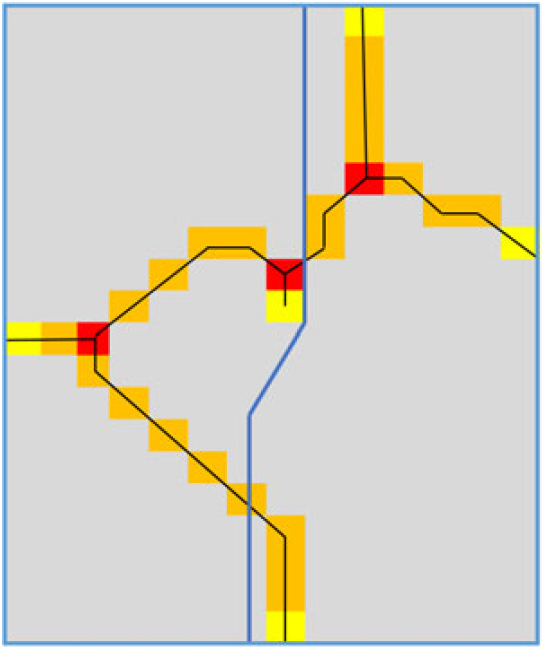
Figure 4. Example for the MIP-based approach: STAR shown in black, sector boundary in blue, heat values are denoted by colours, where a colour of red, orange, and yellow shows a heat value of 3, 2, and 1, respectively.
7.2 VORONOI-based approach
We run our experiments applying the Voronoi-based approach from Section 6 on the routes computed by the MIP presented in Subsection 3.1 (see(Reference Granberg, Polishchuk, Polishchuk and Schmidt10) for the experiments that created these routes). We use the STAR-SID combination from Figure 5(a) as the exemplary routes. In Fig. 5(b) the hotspots, as defined by our controller experts (runway, entry and exit points with high traffic load, and intersection points of SIDs and STARs), are marked: the points A, B, C, D, E, F and O (that is,  \[{\cal H} = \{ A,B,C,D,E,F,O\}\]). The hotspot O is placed on the last merge point before the runway, a hotspot that requires continuous attention; thus, we aim to place it into a separated sector (which is equivalent to assigning O a hotspot weight of
 \[w_O \ge \sum\nolimits_{\eta \in {\cal H}\backslash O} \omega _\eta /(k - 1)\]), depicted in white in the following figures. Points A and C represent TMA entry/exit points. The remaining points (B, D, E, F) mark intersections of STARs and SIDs, where aircraft separation is to be controlled carefully. The closer the intersections is to the runway, the smaller is the vertical aircraft separation, and, as a consequence, the higher is the ATCO taskload associated with this point. We have ω A = ω C = ω D = ω E = ω F = 1, ω B = 2, ω O = 3.
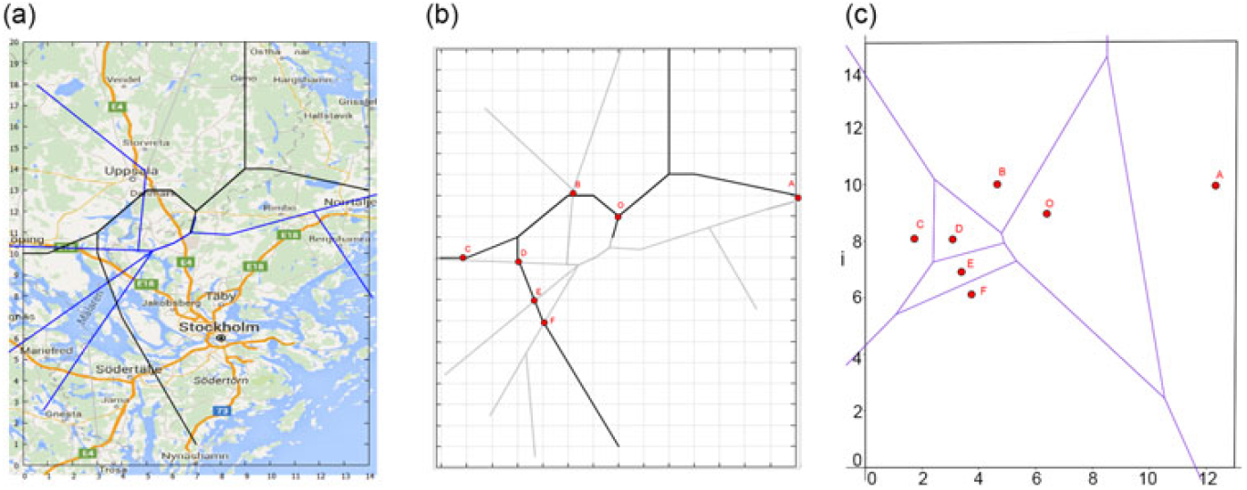
Figure 5. (a) Exemplary SIDs and STARs in Stockholm TMA computed by the MIP presented in Subsection 3.1 overlaid on a map of the Stockholm region in Sweden. (b) The same STARs and SIDs with hotspots marked by red points and letters A, B, C, D, E, F, and O. (c) Voronoi diagram of the hotspots.
The Voronoi diagram for these points is illustrated in Fig. 5(c). We choose k = 4, that is, we want to merge all Voronoi cells except for O into three sectors. We choose this number, because today, the most common sector configuration for Stockholm TMA consists of three sectors, and we want to ensure that it is possible to analyse a higher cardinality, the method is applicable to any k.
First, we aim to balance the sector area. We consider all possible ways to merge the Voronoi cells into three sectors and check the deviations of the total area of the resulting sectors. Here, no combination allows for a perfect area balance among the three sectors, but for three sectorisations we have less than 10% deviation from the average, see Fig. 6. The sectors in Fig. 6(b) are not connected, thus, we report (a) and (c) to be our optimal sectorisations w.r.t. area balance. Both sectorisations feature simple sector shapes and trajectory-based convex sectors. See Fig. 7(a) for an overlay of the sectorisation in (c) and the given routes. All sectors are trajectory-based convex, this also holds for the sectorisation of Fig. 6(a).
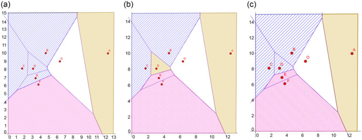
Figure 6. Three sectorisations with sector area that deviates less than 10% from the average.
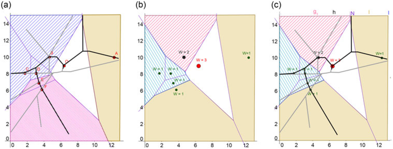
Figure 7. (a) Overlay of routes (STAR in black, SID in gray) and sectors from Fig. 6(c). (b) Sectorisation with balanced taskload, i.e. balanced hotspot weights. (c) Overlay of routes (STAR in black, SID in gray) and sectors from (b).
If we switch to the more important objective of balancing the controller taskload, we use the weights  \[
\omega _\eta \forall \eta \in {\cal H}
\] as defined above. Again, we need to merge the Voronoi cells from Fig. 5(c), and we use k = 4. A perfectly balanced sectorisation is a sectorisation such that
\[
\omega _\eta \forall \eta \in {\cal H}
\] as defined above. Again, we need to merge the Voronoi cells from Fig. 5(c), and we use k = 4. A perfectly balanced sectorisation is a sectorisation such that  \[
\omega _{S_i } = \sum\nolimits_{\eta {\kern 1pt} \in {\kern 1pt} {\cal H}} \omega _\eta /k\;\;\forall S_i \in {\cal S}
\], where w Si = Ση ∈ Si ω η. As
\[
\omega _{S_i } = \sum\nolimits_{\eta {\kern 1pt} \in {\kern 1pt} {\cal H}} \omega _\eta /k\;\;\forall S_i \in {\cal S}
\], where w Si = Ση ∈ Si ω η. As  \[
\sum\nolimits_{\eta {\kern 1pt} \in {\kern 1pt} {\cal H}} \omega _\eta = 10
\] ω η = 10 and k = 4, but we have only integer weights, we cannot achieve a perfect balance. Hence, we have two sectors of weight 2 and two sectors of weight 3. The resulting sectorisation is shown in Fig. 7(b).
\[
\sum\nolimits_{\eta {\kern 1pt} \in {\kern 1pt} {\cal H}} \omega _\eta = 10
\] ω η = 10 and k = 4, but we have only integer weights, we cannot achieve a perfect balance. Hence, we have two sectors of weight 2 and two sectors of weight 3. The resulting sectorisation is shown in Fig. 7(b).
Note that the sector containing hotspots A and F (shaded in brown in Fig. 7(b)) does have a jagged boundary, but it is trajectory-based convex, see Fig. 7(c).
8.0 CONCLUSION AND OUTLOOK
We presented two approaches to simultaneous design of STARs and control sectors in a TMA; both approaches are based on separating the traffic hotspots into different sectors.
The first approach is based on mixed integer programming. This is a powerful, but computationally intensive tool. It combines two of our prior grid-based MIP formulations for TMA sectorisation and for the design of arrival routes. We showed how we can combine these two approaches to a single MIP, and that we can integrate constraints on the interaction between sector boundary and arrival routes, which yields a simultaneuos optimisation of arrival routes and sectors.
The second approach is based on geometric ideas of defining the sector boundaries by edges of a Voronoi diagram of the “hotspots” of ATCO activity on the terminal routes. It uses disjoint disks to separate the potential “hotspots”. The disks must stay disjoint both between themselves and from the sector boundaries; the boundaries can be moved, hence, this approach gives the airspace designer the freedom of re-sectorisation.
We applied the approaches to Stockholm TMA and presented results of the experiments. With these, we demonstrated the feasibility and applicability of both approaches.
It could be interesting to explore the design with more realistic STARs, including, e.g. curved approaches. More generally, we believe that in the prior research the TMA routes were often too simple (RF arcs (radius arc to a fix) were not taken into account, the routes did not reach all the way to the RWYs, etc.), while the sectors, on the contrary, were often overly complicated (so that postprocessing was needed because sector simplicity is hard to enforce as a constraint – simplicity is an elusive notion). We dare to suggest pushing the research in the opposite direction – advanced routing and simple sectors. Indeed, it makes sense to use a dense grid to produce the routes, fine-tune and postprocess them since any mile cut is a lot of fuel saved; on the contrary, sectors boundaries may change locally, at most places, without noticeable effect on ATCOs nor on the flights – if the sectors separate well the hotspots, the exact shape of the sectors is not so important. Moreover, we aim to solve larger instances with the MIP-based approach.
Another possibility for the Voronoi-based approach is to define disks of different size around hotspots, where the size is given by the weight w η, and compute the Voronoi diagram for these disks. Thus, a more intense hotspot would be guaranteed to be further away from sector boundary than the guaranteed distance for lower intensity hotspots.
ACKNOWLEDGEMENTS
This research is funded by the grant 2014-03476 (ODESTA: Optimal Design of Terminal Airspace) from Sweden’s innovation agency VINNOVA and in-kind participation of LFV. We thank Billy Josefsson (project co-PI, LFV) and the members of the project reference group—Eric Hoffman (Eurocontrol), Håkan Svensson (LFV/NUAC), Anne-Marie Ragnarsson (Transportstyrelsen, the Swedish Traffic Administration), Anette Näs (Swedavia, the Swedish Airports Operator), Patrik Bergviken (LFV), Håkan Fahlgren (LFV)—for fruitful discussions.


 Open access