

NOMENCLATURE
- c
blade chord [m]
- C l
lift coefficient
- C d
drag coefficient
- C p
pressure coefficient,
 $
C_p = {{p - p_\infty } \over {{1 \over 2}\rho V_\infty ^2 }}
$
$
C_p = {{p - p_\infty } \over {{1 \over 2}\rho V_\infty ^2 }}
$- C T
thrust coefficient,
$
C_T = {T \over {\rho \pi R^2 (\Omega R)^2 }}
$- D
drag force in disk local coordinate system [N]
- E
total energy [N.m]
- F
instantaneous force vector in the global coordinate system [N]
- Fc
inviscid fluxes
- Fυ
viscous fluxes
- l, b, h
deck length, ship beam, and hangar height [m]
- L
lift force in disk local coordinate system [N]
- L s
ship length [m]
- N
number of blades
- p
pressure [N/m2]
- R
radius of rotor disc [m]
- R
source term [N]
- t
time [s]
- u, ν, w
velocity in three directions [m/s]
- ν rel
flow velocity relative to the blade [m/s]
- V ∞
freestream velocity [m/s]

GREEK SYMBOLS
- α
effective angle of attack [rad]
- θ
blade twist angle [rad]
- ψ
azimuth angle [rad]
- φ
induced angle of attack [rad]
- d ϕ
angular distance [rad]
- θ ro, θ rc, θ rs
collective pitch, lateral cyclic pitch, and longitudinal cyclic angles [rad]
- ρ
fluid density [kg/m3]
- β
logical variable
- Ω
rotor speed [rad/s]
Acronyms
- DES
detached eddy simulation
- LES
large-eddy simulation
- NRC
National Research Council of Canada
- PSD
power spectral density
- RMS
root-mean-square
- ROBIN
Rotor Body Interaction
- SFS
simple frigate shape
- UDF
user-defined function
- URANS
unsteady Reynolds-averaged Navier-Stokes
- WOD
wind-over-deck
1.0 INTRODUCTION
Shipborne helicopters are widely employed by modern navies, and the safety of their launch and recovery has always been a major concern for pilots and researchers(Reference Lumsden, Wlikinson and Padfield1,Reference Lee, Sezer-Uzol, Horn and Long2) . Unlike land-based operations, the restricted landing area just behind the ship’s superstructure makes it difficult to execute the landing manoeuvre. More importantly, when the air passes over the superstructure, highly turbulent flow is formed in the lee of the ship’s superstructure, known as the airwake. This could impose significant unsteady aerodynamic forces and moments on the helicopter, thus making the landing task much more challenging.
Over the past years, a number of numerical studies on ship airwakes have been conducted:Reddy(Reference Reddy, Toffoletto and Jones3) and Syms(Reference Syms4) performed simulations to investigate the general features of the simple frigate shape (SFS) airwake. However, modelling the steady velocity distribution over the flight deck is not sufficient in this application due to the lack of unsteady components. In recent years, the unsteady nature of ship airwakes has been given much attention by researchers. Hodge et al.(Reference Hodge, Zan and Roper5) performed unsteady Reynolds-averaged Navier-Stokes (URANS) simulations of the SFS2 airwake. In addition, detached eddy simulation (DES)(Reference Lawson, Crozon and Dehaze6,Reference Forrest and Owen7) and large-eddy simulation (LES) methods(Reference Thornber, Starr and Drikakis8,Reference Polsky9) were also applied to capture details of the unsteady airwake. Muijden et al.(Reference Muijden and Boelens10) conducted comparative studies between Reynoldsaveraged Navier-Stokes (RANS) and LES simulating the velocity distribution over the flight deck. The results indicated that the RANS method was acceptable for modelling the airwake to an acceptable level of accuracy.
In addition to the simulations of isolate ship airwake, there have been several numerical studies on the aerodynamic interference between ship airwakes and shipborne helicopters. Kääriä et al.(Reference Kääriä, Forrest and Owen11), Scott et al.(Reference Scott, White and Owen12), and Forrest et al.(Reference Forrest, Owen and Padfield13,Reference Forrest, Kääriä and Owen14) employed a one-way coupled strategy to investigate the effect of ship airwake on the aerodynamic loads imparted on a helicopter; however, these studies ignored the rotor-on-ship effect. Bridges et al.(Reference Bridges, Horn and Alpman15) also applied one-way coupling to determine control inputs for a prescribed landing trajectory. However, the results suggested that one-way coupling may obtain unsatisfactory results. This result would seem to imply that it is necessary to conduct two-way coupled simulations. Lee et al.(Reference Lee and Silva16) and Oruc et al.(Reference Oruc, Horn and Shipman17) carried out two-way coupled calculations by using the moving overset mesh method(Reference Meakin18) and momentum source method(Reference Rajagopalan and Mathur19), respectively. The recirculating flow regime, located between hangar and helicopter, was successfully simulated, and the effect of this phenomenon was also analysed. However, the recirculation regime could not be captured by one-way coupling.
All these studies increase the understanding of the effects of ship airwake on helicopters. It should be noted that the influence of rotational direction of the helicopter’s main rotor was not included in the above studies. In fact, because of the large spatial and temporal velocity gradients in the airwake, the relative velocity of the advancing and the retreating side rotor blades is different for rotors which rotate in the opposite direction. How significant the difference might be and what influence this difference has on pilot workload are not clear.
This is the motivation behind conducting the present research. The numerical simulations of coupled flowfield have been carried out to investigate the rotational direction effects on the aerodynamic loading characteristics for two helicopter rotors with opposite rotation directions. First, coupled simulations based on the momentum source method are performed for different landing trajectories. Results in terms of time-averaged thrust and pitch and roll moments are then compared for the two helicopter rotors with opposite rotation directions and root-mean-square (RMS) analysis is used to examine the unsteady loading levels. The turbulence intensity and the distributions of velocity and vorticity for the flowfield are also analysed to explore the origin of the differences in aerodynamic loads. In addition, to study these differences further, the moving overset mesh method was employed to simulate the variation of blade thrust when rotating in the ship airwake with the rotor at certain key locations. Through the present investigation, it is shown that the rotational direction of the main rotor has a significant effect on both the collective control margin and pilot workload.
2.0 NUMERICAL METHODS FOR TWO-WAY COUPLED SIMULATION
2.1 Computational fluid dynamic (CFD) solver
The computations are performed using the commercial software FLUENT. The ship/rotor– coupled flowfield is simulated by solving the RANS equations, discretised by a centre finite volume method in the inertial coordinate system. The integral form of unsteady governing equations can be written as below:
 $${\partial \over {\partial t}}\matrix{
\int\!\!\!\int\!\!\!\int
\cr
V \cr} WdV + \matrix{
\cr
\partial V \cr} (F_c (W) - F_\user2{n} (W))dS = \beta \matrix{
\int\!\!\!\int\!\!\!\int
\cr
V \cr} RdV$$
$${\partial \over {\partial t}}\matrix{
\int\!\!\!\int\!\!\!\int
\cr
V \cr} WdV + \matrix{
\cr
\partial V \cr} (F_c (W) - F_\user2{n} (W))dS = \beta \matrix{
\int\!\!\!\int\!\!\!\int
\cr
V \cr} RdV$$where W is the vector of conserved variables [ρ ρu ρυ ρw ρE]T; ρ, u, υ, w, and E denote the fluid density, velocity in three directions and total energy, respectively. Fc, Fν, and R represent inviscid fluxes, viscous fluxes, and source terms, respectively. β is the logical variable for the rotor model (β = 1 represents momentum source method, and β = 0 is the moving overset mesh method). Both the momentum source method and moving overset mesh method are employed for simulating the ship/rotor–coupled flowfield to satisfy different levels of fidelity requirement.
For the moving overset mesh method, rotors are modelled as the real blades which can flap, pitch, and rotate. Generally, a C-O (or C-H) type grid and a Cartesian grid are used for body-fitted grids of each blade and the background grid, respectively. In the method, a two-step process (i.e., hole cutting(Reference Petersson20) and donor search(Reference Meakin18)) takes place to identify the topological relationship between the background grid and blade grids as shown in Fig. 1. In addition, an interpolation algorithm(Reference Tang21) is adopted to exchange information between the two types of grids.
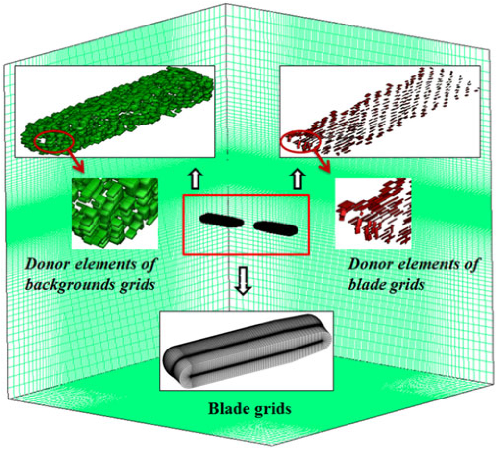
Figure 1. Details of overset grid system.
The momentum source method is realised by employing the user-defined function (UDF) technique provided by FLUENT. In the method, the effect of the rotor is represented by adding source terms to the momentum equations in a disk volume swept by the rotor blades. The source term R in the discretised momentum conservation equations can be written as
 $${\bf{R}} = \left[ {0\;S_x \;S_y \;S_z \;0} \right]^T $$
A UDF code has been written for the calculation of source terms. To determine these source terms, the rotor blades are discretised into spanwise elements, and two-dimensional interpolation grids are generated to model the actual blade elements as shown in Fig. 2. The background grids and interpolation grids are marked, and a sketch of the mapping relationship between the two types of grids is also shown in Fig. 2(b). It can be seen that each element is associated with a number of cells on the background grid. The source terms are calculated per blade element on the interpolation grids and then distributed to the background grid based on an interpolation algorithm. In the two-way coupling method, the information is thus transferred between the local flow conditions and the modelled rotor.
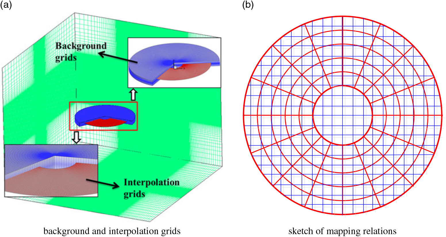
Figure 2. Grids generation and mapping relations; (a) background and interpolation grids; (b) sketch of mapping relations.
During this procedure, it is necessary to calculate the aerodynamic force on each blade element. The first step is to identify the effective angle of attack α, which can be calculated as:
 $$\alpha = \theta _{r0} - \theta _{rc} \cos \psi - \theta _{rs} \sin \psi + \theta - \varphi $$
where θ r0, θ rc, and θ rs are the collective pitch, lateral cyclic, and longitudinal cyclic pitch angles, respectively. θ is the blade twist angle and ψ denotes azimuth angle. φ represents the induced angle of attack that can be calculated by the rotation speed and local flow velocity.
After the effective angle of attack is calculated in the local disccoordinate system, the aerodynamic force coefficients C l, C d can be obtained from lookup tables. The lift and drag forces of the blade element are then computed by:
 $$\matrix{
{L = {1 \over 2} \cdot \rho \cdot \parallel \nu ^{rel} \parallel ^2 \cdot C_l \cdot c \cdot dr} \cr
{D = {1 \over 2} \cdot \rho \cdot \parallel \nu ^{rel} \parallel ^2 \cdot C_d \cdot c \cdot dr} \cr
} $$
$$\matrix{
{L = {1 \over 2} \cdot \rho \cdot \parallel \nu ^{rel} \parallel ^2 \cdot C_l \cdot c \cdot dr} \cr
{D = {1 \over 2} \cdot \rho \cdot \parallel \nu ^{rel} \parallel ^2 \cdot C_d \cdot c \cdot dr} \cr
} $$where ν rel is the flow velocity relative to the blade and c denotes the blade chord. These forces are finally converted into instantaneous force vector −F in the global coordinate system through a series of coordinate transformations, which represents the effect of the blade on the fluid element. Fig. 2 also shows that only a fraction of rotor revolution time will be spent by the blade to pass through a certain control volume. The time-averaging source terms S = (S x, S y, S z), which are added to the momentum conservation equation, should therefore be scaled by the time fraction:
 $$S = - N \cdot {{d\phi ( - F)} \over {2\pi }}$$
where N is the number of blades and dϕ is the angular distance.
FLUENT’s density-based Navier–Stokes solver is used for simulations. The inviscid terms are computed using the second-order upwind Roe scheme(Reference Deconinck, Roe and Struijs22). Temporal integration is performed implicitly using a dual-time stepping method(Reference Pandya, Venkateswaran and Pulliam23). The two-equation k − ω turbulence model(Reference MENTER24) is employed for RANS closure.
2.2 Numerical method validation
Because of a lack of experimental data for the ship/rotor–coupled flowfield, simulations of isolated ship and rotor/fuselage interactions are performed to demonstrate the effectiveness of the method.
1. Isolated ship simulation
In the simulation, the SFS2 model is used due to the availability of experimental data provided by the National Research Council of Canada (NRC). The calculation is carried out with a freestream velocity of V∞ = 12.87 m/s for a headwind. Figure 3 shows the computed time-averaged streamwise velocity distribution over the flight deck compared with the experimental data(Reference Zhang, Xu and Ball25). It is shown that the computed results agree well with the measurements. The results also indicate that the hangar has a large blockage effect on the free stream, thus causing a reduction in the streamwise velocity over the flight deck. The quantitative comparisons are presented in Fig. 4. The line is located at 50% of the flight deck length at hangar height. A corresponding downwash is seen over the flight deck due to flow separation from the hangar. It can be seen that the trends are in agreement although there is some discrepancy in the streamwise velocity component.

Figure 3. Time-averaged streamwise velocity distributions over the flight deck; (a) experiment, (b) CFD calculation.

Figure 4. Comparison of experiment and CFD calculation for velocity components at 50% deck length, plotted at hangar height.
2. Isolated rotor-fuselage simulation
The Georgia Tech rotor-fuselage configuration(Reference Komerath, Mcmahon and Hubbartt26) is used as the validation case(Reference Park, Nam and Kwon27). The rotor operates at a blade tip Mach number of 0.295 and an advance ratio of 0.1. Figure 5 shows the maps of vorticity on four planes based on the momentum source method and moving overset mesh method, respectively. The fuselage is coloured by pressure. The results indicate that, compared to the moving overset mesh method case, the main flow characteristics of coupled rotor/fuselage simulation, such as the concentrated vortex, are well captured by the momentum source method. In Fig. 6, time-averaged surface pressure distributions along the top and bottom of the fuselage are given. Also, the computed results agree well with the measurements. It is clear that due to the tip vortex impingement, two distinct peaks occur along the top of the fuselage.
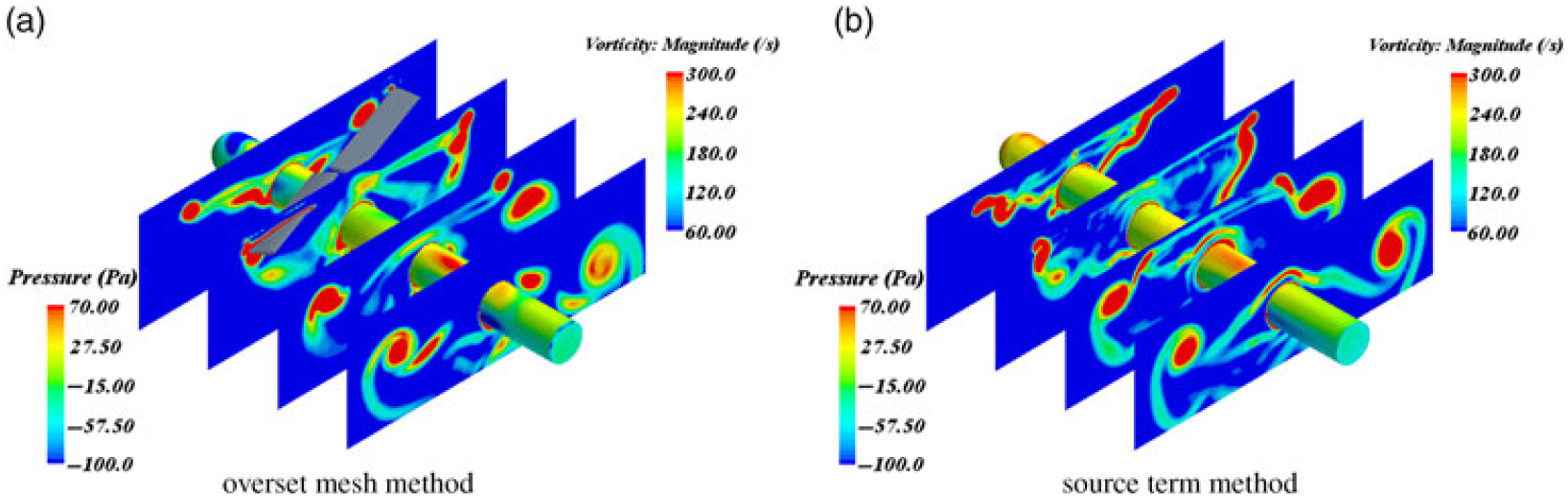
Figure 5. Maps of vorticity on four planes perpendicular to the central axis of the fuselage; (a) overset mesh method, (b) source term method.
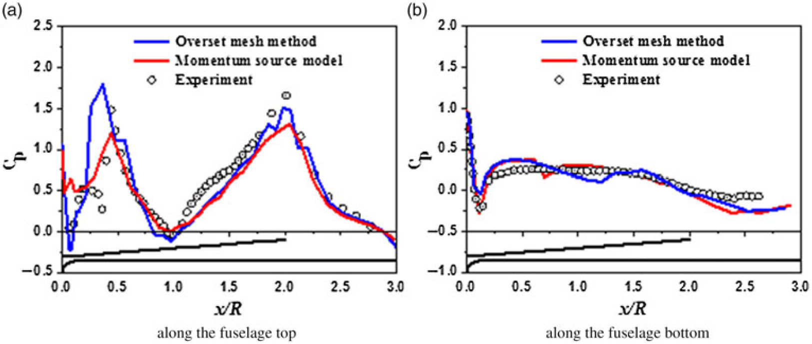
Figure 6. Comparison of experiment and CFD calculation for time-averaged pressure distribution; (a) along the fuselage top, (b) along the fuselage bottom.
3.0 RESULTS AND DISCUSSIONS
3.1 Numerical set-up and data analysis
A 1:10 scale model of the LPD-17 (Fig. 7) and a simple rotor, which has been used in the NASA Langley Rotor Body Interaction (ROBIN) configuration(Reference Raymond and Gorton28), are chosen as they represent a good compromise between geometric realism and mesh complexity. The ship model has a deck length (l) of 6.4 m, a beam (b) = 3.2 m, and a hangar height (h) = 1.6 m, and the ROBIN has a rotor radius (R) of 0.861 m. The rotor rotational speed (Ω) is 209 rad/s and collective pitch angle is 10.3 degrees. The coordinate system used in the computations has its origin at deck level, at the stern, on the ship centreline. The x-direction is positive aft, y is positive to starboard, and z is positive up. This forms a right-handed orthogonal coordinate system.

Figure 7. Sketch of LPD-17 ship model and 17 rotor locations relative to the flight deck.
Two landing trajectories are considered in this study. One represents a lateral traverse through the airwake where the rotor moves from a portside approach position to a hover over the landing spot. The other is a longitudinal translation where the rotor moves from the stern to the mid-deck region. The rotor is placed at 17 points along the two trajectories as shown in Fig. 7, and the rotor’s vertical (z) position is maintained at hangar height throughout the translation. Consistent with naval terminology, winds from starboard are denoted as ‘Green’ and winds from port as ‘Red’(Reference Hodge, Forrest, Padfield and Owen29). At each position, a simulation is performed with a freestream velocity of V ∞=15 m/s at Green 30° wind-over-deck (G30 WOD) angle. In the discussions to follow, velocity and turbulence intensity are normalised by freestream velocity, and the rotor position in (x, y, z) are normalised by deck length (l), ship beam (b), and hangar height (h), respectively.
A 10L sx8L sx8L s rectangular computational domain is generated by commercial software ANSYS ICEM (Fig. 8) where L s is ship length. The ship body and sea surface are designated as no-slip walls; the other five faces are given a Riemann boundary condition to avoid any reflections into the domain. Moreover, a finer mesh topology is created over the flight deck to capture the detailed features of the coupled flowfield. The wall unit values, which represent spacing normal to the ship surface, are set to 2 mm in order to satisfy the requirement of the standard wall function used in the turbulence model; thus, the y+ is within a range of 30~280. Cell counts are approximately 5.2×10⁶ and 8.6×10⁶ for the simulations based on the momentum source model and moving overset mesh method, respectively, reflecting the increasing complexity of the numerical methods.
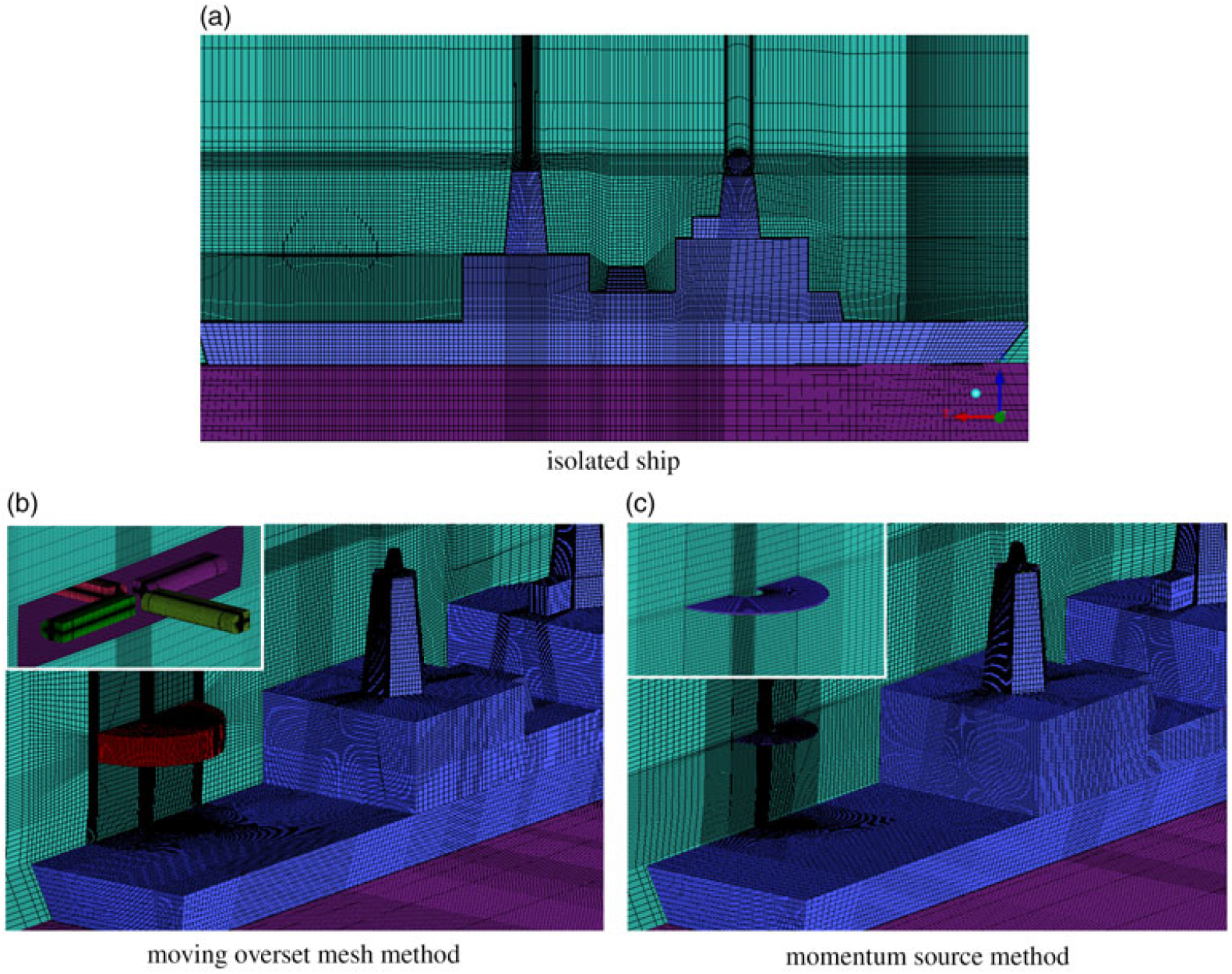
Figure 8. Views of the grids used for ship/rotor–coupled flowfield calculations; (a) isolated ship, (b) moving overset mesh method, (c) momentum source method.
Each simulation employing the momentum source model is initiated by a steady-state solver. The result can be used to initialise the unsteady simulation to speed up the calculation process. The solution convergence is determined by monitoring the residuals. Roughly, 2500 iterations are necessary for convergence. After that, the simulation is restarted for the unsteady calculation. The time step (TS) is set to 0.002 seconds based on the guidelines(Reference Muijden and Boelens10).
A complete unsteady calculation consists of 7,500 TS, with 5,000 used for recording the aerodynamic loads of the rotor and the airwake data. For the simulations using the moving overset mesh method, due to a large difference in frequency between the rotor aerodynamics and the ship airwake, 100 rotor revolutions are required to capture the fully developed coupled flow-field. In each calculation, one revolution is divided into 360 TS, equivalent to 8.33×10⁻⁵ seconds per TS. All the calculations described above are run on a computing cluster (IBM X440) with 24 processors.
After the time-histories of the aerodynamic loads are obtained through the calculations, the RMS method used by Lee and Zan(Reference Lee and Zan30,Reference Lee and Zan31) is employed to analyse the unsteady loading levels. Using this method, power spectral density (PSD) plots are first derived from the time-histories. The square root of the integral between 0.2 and 2.0 Hz is then used as a measure of the unsteady loads, and this quantity will be referred to as the RMS loading (e.g., RMS pitch). The integration is shown graphically in Fig. 9. This frequency band is selected because disturbances in the closed-loop pilot response frequency range of 0.2–2.0 Hz have the greatest impact on pilot workload. Time-averaged analysis of the aerodynamic loads (i.e., rotor thrust and pitch and roll) is also carried out in this paper, and the mean thrust and pitch and roll moments are normalised by ρπR 2(ΩR)2 and ρπR 3(ΩR)2 accordingly. In the following discussion, thrust is positive when acting upward, pitch is positive when the front part of the rotor is nose up, and roll is positive when rolling to the left-hand side (viewed from stern).
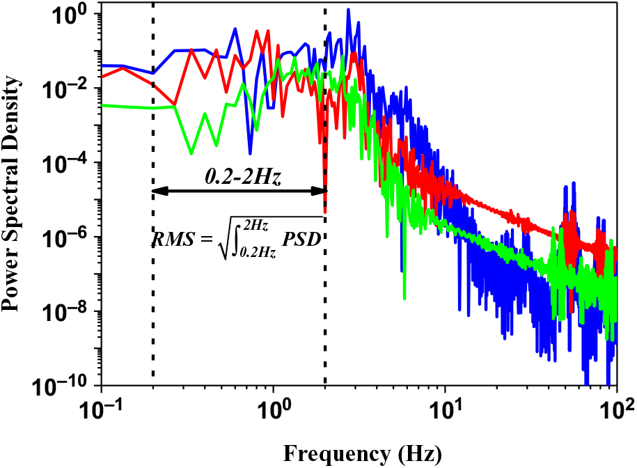
Figure 9. Closed-loop pilot response frequency bandwidth used to define RMS loads.
3.2 Time-averaged aerodynamic loading characteristics
1. Lateral translation
Figure 10 shows the time-averaged aerodynamic loads along the lateral translation path for two helicopter rotors with opposite rotation directions at hangar height in G30 WOD angle. The lateral rotor position, y, is measured from the centre of the deck, so y/b = 0 and y/b = −0.5 represent the locations over the landing spot and port side deck edge, respectively. As can be seen, there is a significant difference in thrust between −1 <y/b< −0.375, where the mean thrust of the counterclockwise rotor is 10–20% higher than that of the clockwise rotor in this area. Moreover, the thrusts of the two rotors are both less than that of the baseline rotor (CT = 0.00292), which is immersed in a freestream of 15 m/s without the presence of the ship, during the entire lateral translation. This suggests that for a landing manoeuvre in a G30 WOD when operating a helicopter with a clockwise rotor, the pilot would be required to demand more collective pitch to maintain the desired altitude above the flight deck. That is to say, the helicopter with the clockwise rotor provides less collective control margin in such conditions, thus making it more difficult for the pilot to compensate for any unsteady disturbances in the vertical axis.
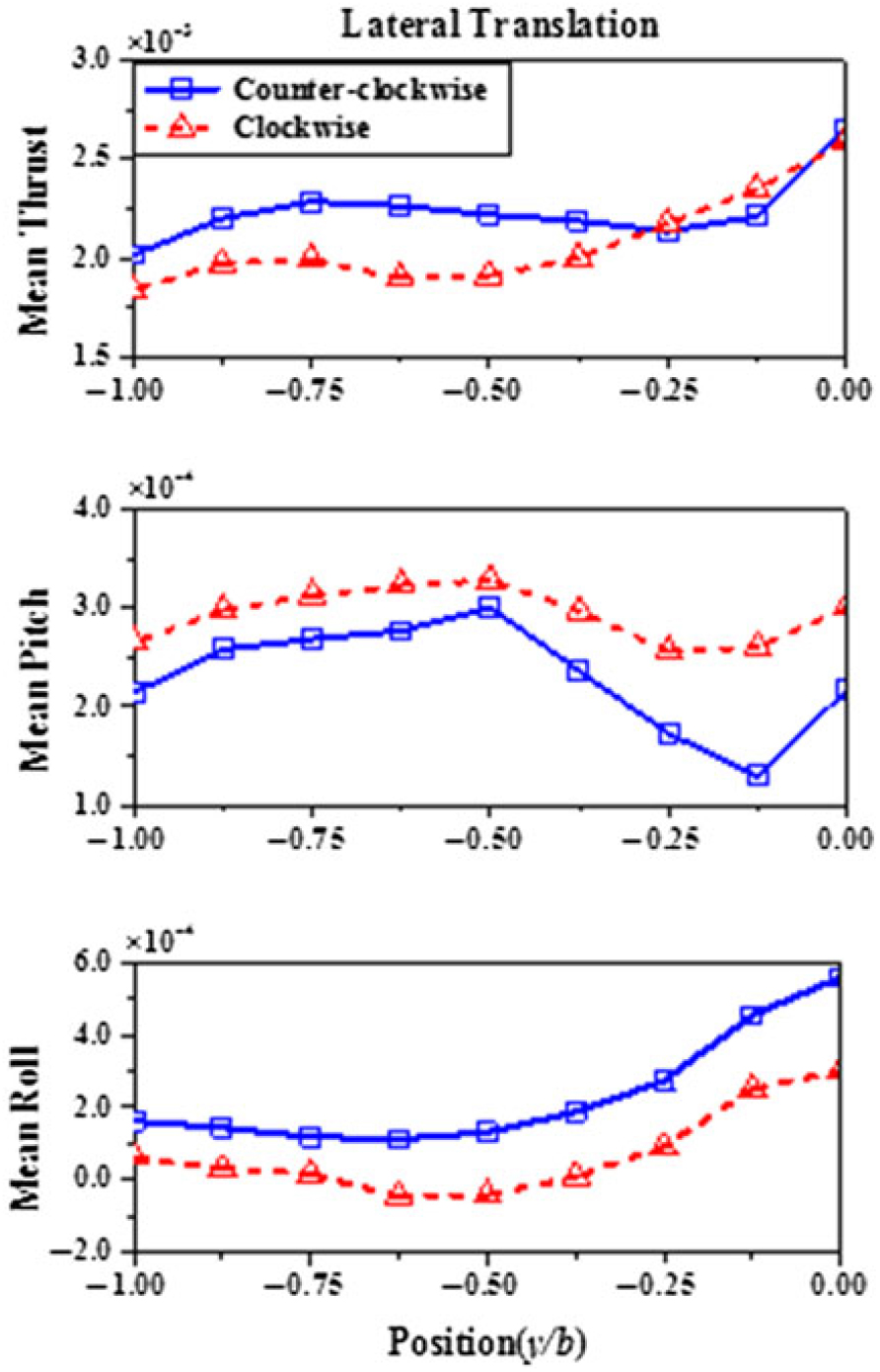
Figure 10. Mean thrust and pitch and roll characteristics for counterclockwise rotor and clockwise rotor in lateral translation.
The origin of this difference can be identified by studying the flow characteristics of the ship airwake. Figure 11 shows isosurfaces of vorticity over the flight deck, with four distinct flow features highlighted. Features (a), (b), (c), and (d) represent the starboard deck-edge vortex, hangar edge shear layer, helical secondary superstructure vortex, and mast edge shear layer, respectively. As explained by Forrest(Reference Forrest and Owen7), the feature (b) is a main contributing factor to turbulence below the hangar height, while the feature (c) is responsible for most of the turbulence above hangar height.
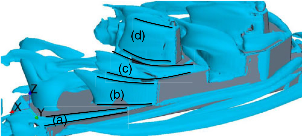
Figure 11. Iso-surfaces of vorticity over the flight deck for G30 WOD condition.
Figure 12 shows contours of mean longitudinal velocity and vertical velocity at hangar height in which the location of the swept area of the rotor disc is indicated for the portside position (y/b = −0.5) and the landing spot hover position (y/b = 0). To improve understandability, the rotating direction of the counterclockwise rotor has also been shown in Fig. 12. It can be seen that the air passes through a narrow region between feature (c) and feature (d) and then divides the flowfield into three parts (Fig. 12(a)), denoted by region 1, region 2, and region 3, respectively. In addition, due to the effect of the helical secondary superstructure vortex, two distinct areas of opposite vertical velocity are formed in the mid-deck region (Fig. 12(b)). When the rotor translates from the region 1 and moves close to region 2, the advancing blades of the counterclockwise rotor (viewed from the stern) are in the higher velocity wake region and the retreating blades are in the lower velocity wake region (Fig. 12a), but the opposite is true for the clockwise rotor. Thus, the relative speeds of the advancing and retreating sides of the counterclockwise rotor are both higher than that of the clockwise rotor. For this reason, the thrust of the former is higher than that of the latter between -1<y/b< -0.375.
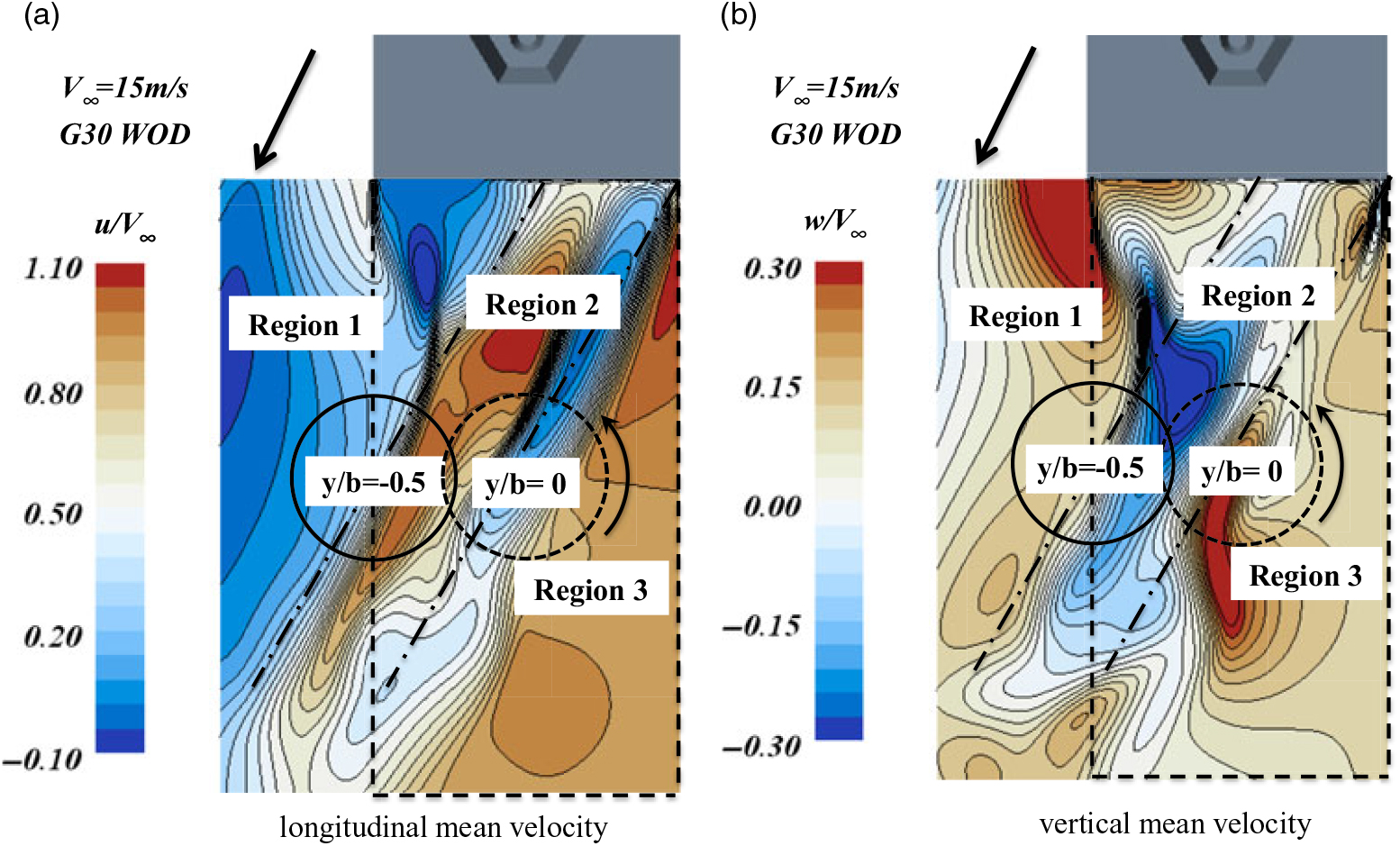
Figure 12. Contours of velocity in a plane at hangar height for G30 WOD condition; (a) longitudinal mean velocity, (b) vertical mean velocity.
In addition to thrust, Fig. 10 also shows the mean pitch and roll moments during the lateral traverse. Like the increase in lift between −0.375 <y/b< −0.125, there is also a sharp increase in roll (towards portside) moment when the right part of the rotor moves into the high upward vertical velocity region (Fig. 12b). These behaviours are consistent with the experimental study of Kääriä(32) and are associated with the phenomenon called the ‘pressure-wall’, which has been observed during at-sea flight testing(33). The pressure-wall can cause a severe reduction in sideslip velocity and even direct the helicopter away from the landing spot. The pilot therefore has to increase the lateral cyclic control input to counteract these adverse effects and maintain an appropriate velocity towards the landing spot. Moreover, the area in which the pressure-wall takes effect often corresponds to the highly turbulent region. This will be analysed further in the next section.
Unlike the variations in thrust and roll moment, between −0.5 <y/b< −0.125, a significant decrease in pitch moment is observed as the rotor is gradually immersed in the high downward vertical velocity region (Fig. 12(b)). This is equivalent to adding a negative pitch moment (nose down) to the rotor that would push the helicopter towards the hangar. This conclusion also concurs with pilot comments that the aircraft is pulled towards the hangar during simulated flight trials(Reference Forrest, Owen and Padfield13). Furthermore, Fig. 12(b) also shows that in this region, the advancing side of the counterclockwise rotor is immersed in a region of upward vertical velocity while the retreating side is exposed to downward vertical velocity; thus, the difference in lift between the advancing and retreating side is exaggerated. However, the opposite is true for the clockwise rotor, so the counterclockwise rotor suffers a sharp reduction of 57% in pitching moment, i.e., an equal increase in nose-down moment, while only a 20% reduction is seen for the clockwise rotor (Fig. 10). This implies that the effect of the aircraft being pulled towards the hangar will be more severe on helicopters with a counterclockwise rotor.
2. Longitudinal translation
Figure 13 shows the time-averaged aerodynamic loading coefficients against longitudinal deck position for the two types of rotors. Again, distinct differences between the two rotors exist in the longitudinal translation. Although a sharp reduction in thrust occurs as the rotor moves into the lower velocity region, the thrust of the counterclockwise rotor is 3–5% greater than that of the clockwise rotor. As with the analysis in the lateral translation case, this is because the relative speeds of the advancing and retreating sides of the counterclockwise rotor are both higher than that of the clockwise rotor.
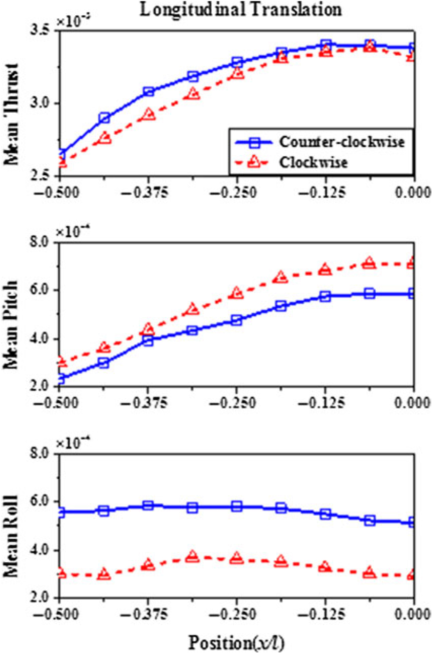
Figure 13. Mean thrust and pitch and roll characteristics for counterclockwise rotor and clockwise rotor in longitudinal translation.
Like the reduction in lift, a significant decrease in mean pitch moment also occurs for both types of rotors. During the entire longitudinal translation phase, the mean pitch has reduced by 57% and 60% for the clockwise and counterclockwise rotor (Fig. 13), respectively. Again, the counterclockwise rotor suffers more decrease. This implies that the helicopter with a counterclockwise rotor is more likely to be pulled towards the hangar in Green oblique wind angles. In addition to this, Fig. 13 also shows that the thrusts of the counterclockwise rotor and clockwise rotor, on average, are 10% and 6% higher than that of the baseline rotor, respectively. It means that landing a helicopter from the stern can provide more collective control margin for the pilot. This is quite favourable for counteracting the unsteady disturbances in vertical direction.
3.3 Unsteady aerodynamic loading characteristics
In the previous section, differences in the time-averaged loading characteristics between the two helicopter rotors with opposite rotation directions for two different approach paths were identified, and the impact of the differences on the pilot’s control inputs were also discussed. However, the ship airwake is unsteady in nature and contains different scales of time-varying turbulent structures, which could induce instantaneous perturbations in the loading characteristics of the rotor disk. As a result, the time-histories show large fluctuations in thrust for both rotor types (Fig. 14(a)). Spectral analysis shows that there is significant energy in the fluctuations within the pilot closed-loop response frequency bandwidth of 0.2–2.0 Hz (Fig. 14(b)). Moreover, distinct differences exist between the two PSD plots, especially within 0.2–2.0 Hz. Thus, it is reasonable to expect that the differences in the unsteady loading characteristics are also in existence between the two types of rotors. In this section, the RMS forces and moments for the two rotors are analysed to explore these differences.
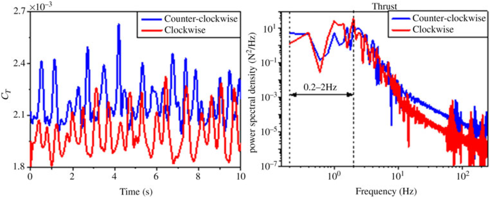
Figure 14. The unsteady loading characteristics of the rotors at y/b = −0.5; (a) time-histories of thrust coefficient, (b) power spectral density plots of thrust.
1. Lateral translation
Figure 15 shows unsteady loading variations through the lateral translation for a G30 WOD angle. It can be seen that there are noticeable increases in RMS loads in all three axes as the rotor moves into the flight deck region. Furthermore, as expected, obvious differences in unsteady loads also exist between the two rotors, especially in the latter stages of the lateral translation over the flight deck, between −0.5 <y/b< −0.125. The RMS thrust and pitch and roll of the clockwise rotor are, on average, 49%, 44%, and 30% greater than those of the counterclockwise rotor, respectively. These results imply that a helicopter with a clockwise rotor will tend to suffer more disturbances during a lateral translation in a G30 WOD condition, especially over the flight deck. Furthermore, this area also corresponds to a region of reduced collective control margin for the clockwise rotor as discussed in the time-averaged analysis. Therefore, the higher degree of unsteady loads will be compounded by reduced collective control margin as well as the pressure-wall effect for the helicopter with a clockwise rotor. This will make it more difficult for the pilot to compensate for disturbances and stabilise the aircraft.

Figure 15. RMS thrust and pitch and roll characteristics for counterclockwise rotor and clockwise rotor in lateral translation.
To identify the reasons behind these differences, it is necessary to investigate the coupled flow features over the flight deck. Figure 16 gives the maps of vorticity at hangar height for various rotor positions. For brevity, only results from the counterclockwise rotor case are presented, because the main flow characteristics are similar for the two rotors. There are three kinds of vortical structures dominating the flowfield over the flight deck, denoted by V1, V2, and V3 in the figure, respectively. The vortical structure V1 is generated from a vertical shear layer emanating from the leeward vertical hangar edge, and V3 is a combined product of the hangar edge shear layer and helical secondary superstructure vortex (i.e., features (b) and (c) as shown in Fig. 11). V2 is constrained in the recirculation zone behind the hangar and changes little over time. The dashed lines in Fig. 16 represent the approximate propagation paths for V1 and V3. When animated, these vortical structures V1 and V3 are seen to propagate downstream and interact with the rotor disc, causing large perturbations in the aerodynamic loads of the rotor.
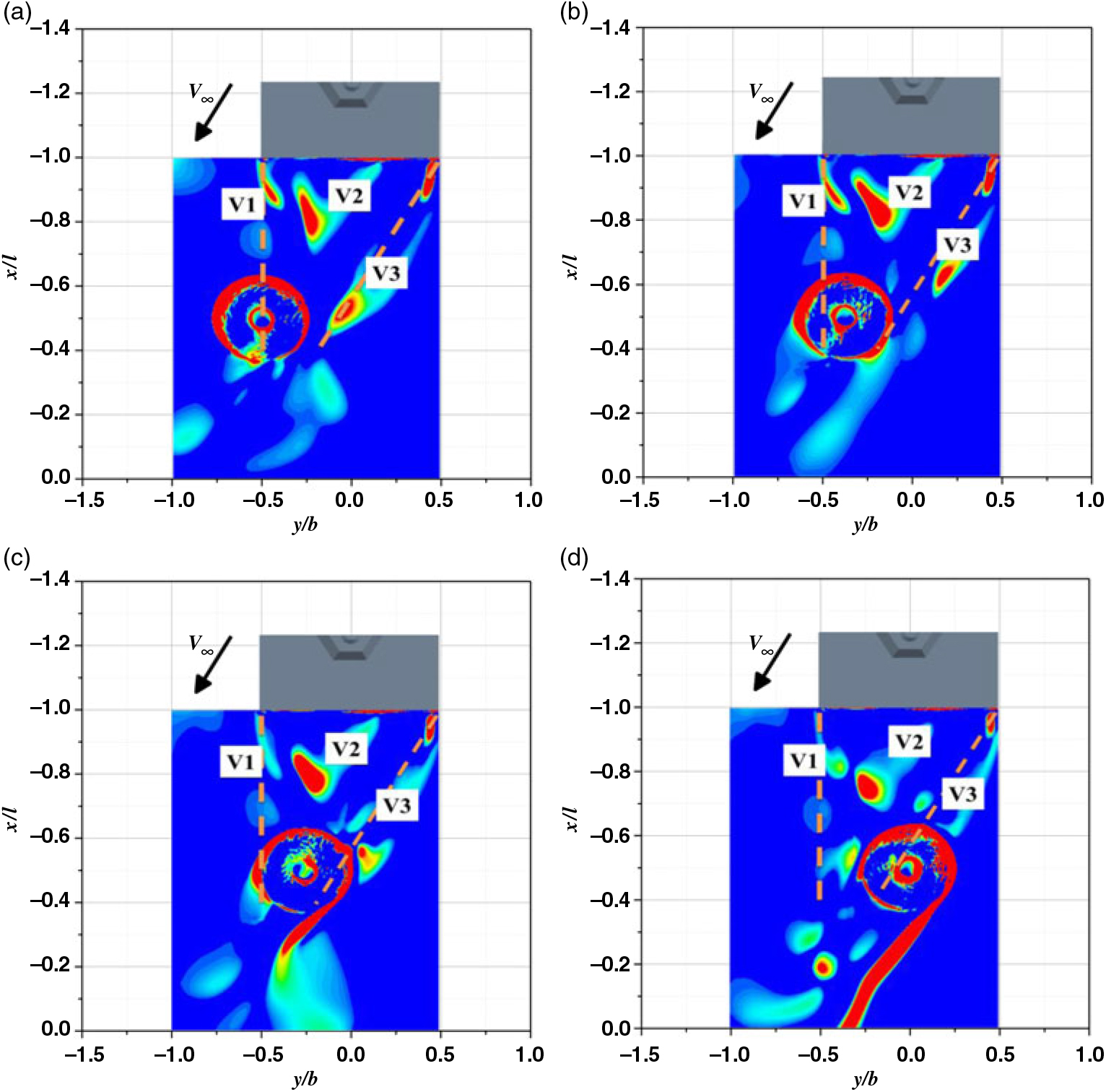
Figure 16. Maps of vorticity for four different lateral rotor positions at hangar height for G30 WOD condition; (a) y/b = −0.5, (b) y/b = −0.375, (c) y/b = −0.25, (d) y/b = 0.
As the rotor moves along the lateral translation path, between −0.5 <y/b< −0.25, the front-left section of the rotor is gradually immersed in the wake of V1, and the right part begins to interact with V3 (Fig. 16(b)). For this reason, sharp increases in RMS loads are observed for both rotors. Moreover, the front-left section is just the advancing side region of the clockwise rotor, so it will suffer more severe disturbances compared with the counterclockwise rotor. This causes the RMS loading levels of the clockwise rotor to be greater than that for the counterclockwise rotor.
When the rotor continues to move towards the mid-deck position, between −0.25 <y/b<0, the front-left section of the rotor gradually moves out of the wake of V1 (Fig. 16(c)), so unsteady loading levels reduce considerably except for the RMS pitch for the counterclockwise rotor. At y/b = 0, only the right part of the rotor (i.e., the advancing side of the counterclockwise rotor) is exposed to V3 (Fig. 16(d)); thus, the RMS loads of the counterclockwise rotor are instead higher than that of the clockwise rotor. Figure 15 also shows that the peak RMS pitch for the counterclockwise rotor occurs at y/b = 0 over the landing spot. At this location, the advancing blades of the counterclockwise rotor are immersed in the wake of vertical structure V2 as shown in Fig. 16(d). Because of the 90° phase shift, these interactions will manifest themselves as disturbances in pitch resulting in a peak RMS pitching moment over the landing spot.
In order to examine these interactions further, the overset mesh method is also employed to analyse the aerodynamic loading characteristics of the blades during the process of rotation. Figure 17 shows the variations of the blade thrust (normalised by ρπR 2(ΩR)2) in the rotating process at y/b = −0.5 over the port edge of the deck. For brevity, only the data for five rotor revolutions are presented. It is clear that the perturbations in blade thrust are much stronger for the clockwise rotor, and these disturbances mainly occur on the advancing side of the rotor disc. In addition, the average blade thrust of the counterclockwise rotor is greater than that of the clockwise rotor. These results are consistent with the conclusions obtained by the momentum source method. This also confirms that the momentum source method is a practical way to investigate the unsteady aerodynamic loading characteristics of a rotor in a ship’s airwake.
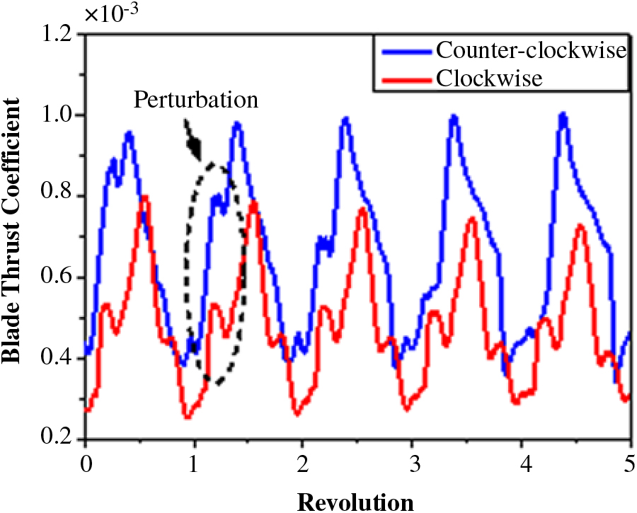
Figure 17. Variation of blade thrust coefficient for five revolutions.
2. Longitudinal translation
The variations of RMS loads across the longitudinal translation path are shown in Fig. 18. As the rotor moves along the ship centreline, obvious increases in RMS loading levels occur for both rotors. Similarly, notable differences are also observed during the longitudinal translation. The RMS thrust and pitch and roll of the clockwise rotor are, on average, 22%, 25%, and 30% greater than those of the counterclockwise rotor, respectively, between −0.375 < x/l < −0.1875. As with the lateral translation case, this suggests that a helicopter with a clockwise rotor will tend to experience more unsteady disturbances during this manoeuvre.
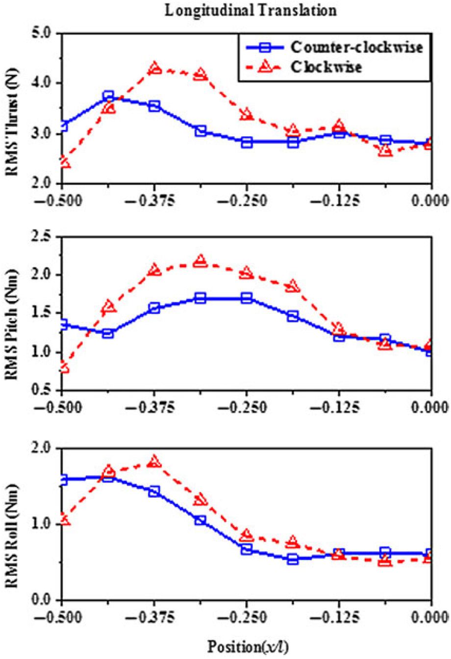
Figure 18. RMS thrust and pitch and roll characteristics for counterclockwise rotor and clockwise rotor in longitudinal translation.
In order to explore the reasons behind these variations in RMS loads, Fig. 19 presents contours of longitudinal and vertical turbulence intensity in a plane at hangar height. The location of the swept area of the rotor disc has been indicated for y/b = −0.1875. It is evident that the rotor is gradually immersed in the highly unsteady region of the air-wake as it moves towards the mid-deck position, so the unsteady loading levels increase considerably for both rotors, especially between −0.375 < x/l < −0.1875.
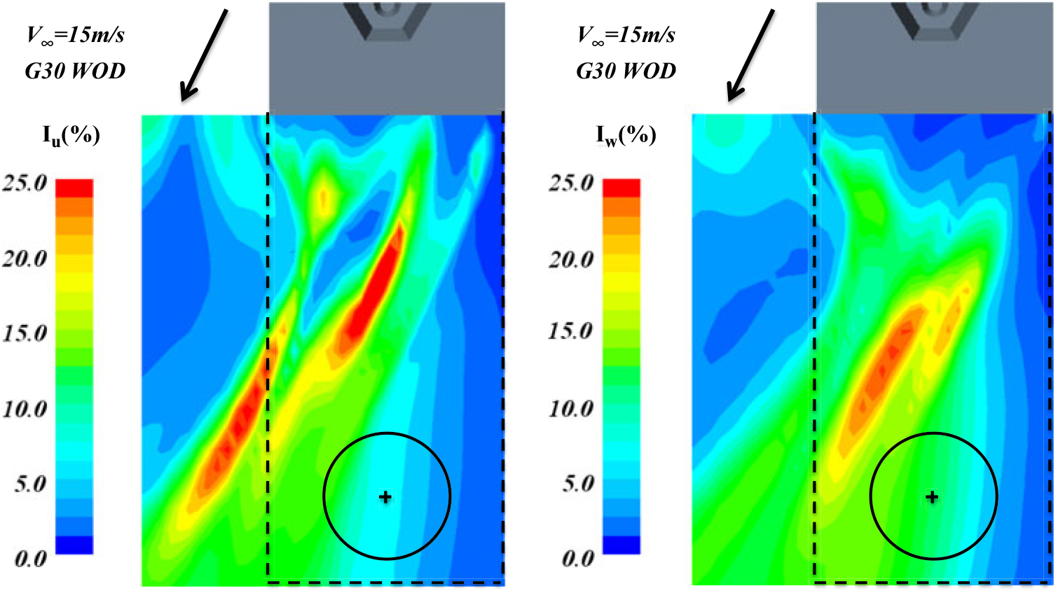
Figure 19. Contours of turbulence intensity in a plane at hangar height for G30 WOD condition; (a) lateral turbulence intensity, (b) vertical turbulence intensity.
The contours of turbulence intensity can indicate which regions are likely to suffer high levels of turbulence. However, they cannot identify the origin of the differences in RMS loads between the two rotors. Therefore, maps of vorticity for different rotor positions at hangar height are shown in Fig. 20, where only the results for the counterclockwise rotor are presented. When the rotor moves forward, the front-left section of the rotor (i.e., the advancing side of the clockwise rotor) encounters the vertical structure V3 first (Fig. 20(b)), thus causing obvious differences in RMS loads between the two rotors. As the rotor continues to move close to the mid-deck position, the front-left section of the rotor is no longer interacting with V3, and only the right part (i.e., the advancing side of the counterclockwise rotor) is immersed in the wake of V3 (Fig. 20(d)), so the RMS loads of the counterclockwise rotor are higher than that of the clockwise rotor over the landing spot.

Figure 20. Maps of vorticity for four different longitudinal rotor positions at hangar height; (a) x/l = −0.1875, (b) x/l = −0.3125, (c) x/l = −0.4375, (d) x/l = −0.5.
4.0 CONCLUSIONS
Numerical studies of the rotational direction effects on a shipborne helicopter rotor have been conducted in a G30 wind-over-deck condition using both the momentum source and moving overset mesh methods. Results in terms of time-averaged and RMS loads are discussed to identify the differences in aerodynamic loading characteristics between the two helicopter rotors with opposite rotation directions. The influence of landing trajectory on these differences is also considered in the paper. From the above discussion, the following conclusions can be drawn:
(1) In current cases, the mean thrust of the counterclockwise rotor, on average, is 15% greater than that of the clockwise rotor in the lateral traverse case and 4% in the longitudinal translation case. This suggests that a helicopter with a counterclockwise rotor could provide more collective control margin.
(2) Although a sharp decrease in thrust occurs as the rotor moves along the centreline of the ship, the mean thrust in the longitudinal translation case is still much greater than that in the lateral translation case. This means that landing a helicopter from the stern can significantly increase the collective control margin available to the pilot.
(3) During the lateral and longitudinal translation phases, there is a more significant reduction in pitch moment for the counterclockwise rotor compared with that of the clockwise rotor. Therefore, the effect of the aircraft being pulled towards the hangar tends to be more severe on a helicopter with a counterclockwise rotor.
(4) The RMS loading levels of the clockwise rotor are much higher than those of the counterclockwise rotor in all three axes for both landing trajectories. In addition, the higher degree of unsteady loads will be compounded by a reduction in collective control margin in addition to the pressure-wall effect during the lateral translation, thus making it more difficult for the pilot to operate a helicopter with a clockwise rotor in G30 WOD conditions.
Although the rotor’s rotational direction is shown to have an obvious influence on the aerodynamic loading characteristics of a shipborne helicopter for the two landing trajectories, it should be reiterated that the simulations have so far been performed for only a single Green 30 WOD condition. More work is needed to identify the influence of rotor rotation direction at different WOD conditions.
ACKNOWLEDGEMENTS
This work was supported by Postgraduate Research & Practice Innovation Program of Jiangsu Province (grant number KYCX18_0312).


 Open access