


Introduction
World biofuel production has risen dramatically in the last 25 years. Opponents of first-generation biofuels claim that the technology diverts agricultural land away from food production for use as a fuel source. Critics point to rising staple food prices during the 2007–2008 world food crisis as evidence of the unintended costs of biofuel expansion (Mitchel, Reference Mitchel2008). The global expansion of crude oil production – driven by fracking technology and the rise of shale oil – has subsequently quelled some of these concerns and led to the United States (US) becoming virtually self-sufficient in crude oil. However, the “food versus fuel” debate remains: To what extent do biofuels really make food prices more susceptible to changes in crude oil markets and prices? In this paper, we seek to disentangle the effects of biodiesel incentives and shale oil expansion on the long-run equilibrium price relationship between crude oil and biodiesel feedstocks.
The literature is somewhat contradictory regarding the relationship between crude oil and edible vegetable oil prices. Yu, Bessler, and Fuller (Reference Yu, Bessler and Fuller2006) study the long-run equilibrium relationships between oilseed prices (soybean, sunflower, canola, and palm) and world crude oil prices between January 1999 and March 2006. The authors find that crude oil prices do not significantly impact oilseed prices over the period of analysis. Later work by Zhang et al. (Reference Zhang, Lohr, Escalante and Wetzstein2010) and Filip et al. (Reference Filip, Janda, Kristoufek and Zilberman2019) give results that are consistent with Yu, Bessler, and Fuller (Reference Yu, Bessler and Fuller2006).
Abdel and Arshad (Reference Abdel and Arshad2008) also investigated the long-term relationship between the prices of petroleum and vegetable oil prices represented by palm, soybean, sunflower, and canola oil prices, using data from January 1983 through March 2008. In contrast to Yu, Bessler, and Fuller (Reference Yu, Bessler and Fuller2006), Abdel and Arshad (Reference Abdel and Arshad2008) find strong evidence of a long-run equilibrium relationship between oilseed and petroleum prices. Consistent with Abdel and Arshad (Reference Abdel and Arshad2008), Ghaith and Awad (Reference Ghaith and Awad2011) and (Esmaeili and Shokoohi (Reference Esmaeili and Shokoohi2011) find evidence of long-term relationships between crude oil and a broader set of food commodity prices, using longer time series ending in the mid-2000s. Hassouneh et al. (Reference Hassouneh, Serra, Goodwin and Gil2012) use data from November 2006 to October 2010 to show the existence of a long run, equilibrium relationship between biodiesel, sunflower, and crude oil prices.
An important limitation of this research is that it fails to account for changes in equilibrium dynamics among biodiesel feedstock and crude oil prices in light of the expansion of biofuel production and growth in the crude oil supply due to shale oil extraction. These factors fundamentally alter market relationships Drabik, De Gorter and Timilsina (Reference Drabik, De Gorter and Timilsina2014). For example, Schaefer et al. (Reference Schaefer, Myers, Johnson, Helmar and Radich2021) find that – partially as a result of biodiesel policy – price premiums for canola oil and sunflower oil have increased by 28% and 4%, respectively, relative to soy oil over the past two decades.
We estimate a series of bivariate models to measure the cointegrating relationship between prices for primary biodiesel feedstocks and crude oil in the US and European Union (EU). Our specifications allow us to test for and distinguish the impacts of two types of structural breaks in these equilibria – (1) smooth shifts driven by the expansion of the global crude oil supply and (2) sharp breaks resulting from the promulgation of the major biofuels legislation (Enders and Holt, Reference Enders and Holt2012).
Our results are connected to the theoretical literature on the impacts of biodiesel production incentives on oilseed and crude oil price relationships. Drabik, De Gorter and Timilsina (Reference Drabik, De Gorter and Timilsina2014) construct a theoretical model to analyze the effects of biodiesel mandates and exogenous diesel price shocks on world soybean and canola markets. The authors find that the jointness in crushing oil and meal from the oilseed reduces the size of the link between diesel and oilseed prices. An increase in the diesel price leads to higher canola prices, but the effect on soybean prices is ambiguous and depends on relative elasticities of meal demand and canola supply because canola produces more oil than soybeans.
We find that the promulgation of the 2005 Energy Policy Act in the US substantially increased the responsiveness of biodiesel feedstocks prices to crude oil price shocks. However, in recent years, expansion in the global supply of crude oil has overshadowed the effects of US biodiesel incentives and blending mandates. In the EU, the Indirect Land Use Change (ILUC) Directive of 2015 substantially reduced the responsiveness of biodiesel feedstock prices to crude oil price shocks.
Background
Production and use of biodiesel have risen dramatically over the last 25 years (Figure 1). The two largest producers of biodiesel are the US and the EU. In the EU, growth in biodiesel was initially incentivized through the Biofuels Directive of 2001 (Directives 2001/77/EC) in October 2001, which required 5.75% of all transport fuels to be replaced by biofuels by the end of 2010. The 2009 Renewable Energy Directive, enacted in April 2009, provided additional support by raising binding targets to 20% renewables for total energy use and 10% for transportation fuel by 2020. In 2015, the European Parliament passed the ILUC Directive (Directive 2015/1513) in September 2015, which requires GHG emissions caused from land use change. In effect, this policy greatly reduces the share of agricultural land in the EU that can be devoted to biofuels feedstocks. Canola oil is the primary feedstock used in EU biodiesel production (47% production share), followed by palm oil (15% production share) and soy oil (7% production share) (Kim, Hanifzadeh and Kumar, Reference Kim, Hanifzadeh and Kumar2018).

Figure 1. Global crude oil and biodiesel production. Global crude oil production and US biodiesel production data in panel (c) are obtained from the US Energy Information Administration (EIA). US biodiesel production is converted from barrels to metric tonnes using a conversion factor of 0.1364. EU biodiesel production data in panel (c) are obtained from the EU Biofuels Annals (various years) GAIN Reports provided by the USDA Foreign Agricultural Service. Production shares for US and EU biodiesel feedstocks are obtained from Kim, Hanifzadeh and Kumar, Reference Kim, Hanifzadeh and Kumar2018.
In the US, the watershed legislation was the Energy Policy Act of 2005 (Public Law 109-58) enacted in August 2005. This legislation required the blending of ethanol and biodiesel into transportation fuels under the Renewable Fuel Standard (RFS). This legislation provided a huge boost to biofuel demand. Usage grew by more than 300% from 2004 (55000 metric tons of biodiesel per month) to 2005 (180 000 metric tons of biodiesel per month) and increased by almost 1000% from 2004 to 2006 (497 000 metric tons of biodiesel per month). In December 2007, the Energy Independence and Security Act of 2007 (Public Law 110-140) further expanded and extended the RFS to require the use of 29.25 million tonnes of biofuel in 2008, increasing to 117 million tonnes by 2022. Soy oil is the primary biodiesel feedstock in the US (55% production share), followed by corn oil (12% production share) and canola oil (10% production share) (Kim, Hanifzadeh and Kumar, Reference Kim, Hanifzadeh and Kumar2018).
Alongside the growth in biofuels, global crude oil production has expanded from approximately 3.7 billion tonnes in 2000 to almost 4.6 billion tonnes in 2019. The increase in crude oil supply is primarily the result of shale oil. After a dormancy period of more than 20 years, shale oil extraction in the US restarted in 2003. The Energy Policy Act of 2005 formally allowed a commercial leasing program, which promoted the extraction of shale oil and oil sands. This expansion has led the US becoming virtually self-sufficient in crude oil.
Conceptual framework
Figure 2 provides a conceptual framework to illustrate the effects of biodiesel incentives and shale oil expansion on the long-run equilibrium price relationship between crude oil and biodiesel feedstocks.Footnote
1
For simplicity, we assume that soy oil is produced via fixed proportions technology using two inputs: (1) crude oil (as a transportation fuel) and (2) a composite input denoted “other”, which represents all other inputs into soy oil production. Thus, the marginal cost of soy oil production is $M{C^{SOY}} = {P^{WTI}} + {P^{OTHER}}$
. In Figure 2, we assume farmers can obtain crude oil for use in soy oil production at a constant marginal cost
$M{C^{SOY}} = {P^{WTI}} + {P^{OTHER}}$
. In Figure 2, we assume farmers can obtain crude oil for use in soy oil production at a constant marginal cost $P_0^{WTI}$
. The input supply of the “other” input (denoted
$P_0^{WTI}$
. The input supply of the “other” input (denoted ${S^{OTHER}}$
in Figure 2) is upward sloping for soy oil producers. The supply of soy oil (denoted
${S^{OTHER}}$
in Figure 2) is upward sloping for soy oil producers. The supply of soy oil (denoted $S_0^{SOY}$
) is the vertical sum of the supply schedules for these two inputs. Prior to the introduction of biodiesel production incentives and blending mandates, demand for soy oil is described by the schedule
$S_0^{SOY}$
) is the vertical sum of the supply schedules for these two inputs. Prior to the introduction of biodiesel production incentives and blending mandates, demand for soy oil is described by the schedule ${D_0}$
in Figure 2. Under these assumptions, soy oil market equilibrium occurs at a price
${D_0}$
in Figure 2. Under these assumptions, soy oil market equilibrium occurs at a price $P_0^{SOY}$
.
$P_0^{SOY}$
.
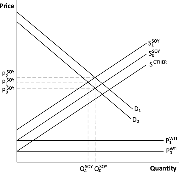
Figure 2. Market for soy oil.
Now suppose an exogenous shock to the crude oil industry shifts the price of crude oil from $P_0^{WTI}$
to
$P_0^{WTI}$
to $P_1^{WTI}$
. This also shifts the supply of soy oil from
$P_1^{WTI}$
. This also shifts the supply of soy oil from $S_0^{SOY}$
to
$S_0^{SOY}$
to $S_1^{SOY}$
, leading to a new equilibrium in the soy oil market at price
$S_1^{SOY}$
, leading to a new equilibrium in the soy oil market at price $P_1^{SOY}$
. Thus, prior to the introduction of biodiesel production incentives and the expansion of shale oil production, the long-run equilibrium relationship between crude oil and soy prices is described by the elasticity:
$P_1^{SOY}$
. Thus, prior to the introduction of biodiesel production incentives and the expansion of shale oil production, the long-run equilibrium relationship between crude oil and soy prices is described by the elasticity:
 $$\eta _{WTI}^{SOY} \approx {{\Delta {P^{SOY}}} \over {\Delta {P^{WTI}}}} \times {{{P^{WTI}}} \over {{P^{SOY}}}} = {{P_1^{SOY} - P_0^{SOY}} \over {P_1^{WTI} - P_0^{WTI}}} \times {{P_0^{WTI}} \over {P_0^{SOY}}}$$
Effects of biodiesel production incentives and blending mandates
We use equivalent comparative statics to deduce the impacts of biodiesel production incentives and blending mandates. Initial equilibrium (in which crude oil prices are $P_0^{WTI}$
) occur at the same point as before. However, an exogenous shock to the crude oil price from
$P_0^{WTI}$
) occur at the same point as before. However, an exogenous shock to the crude oil price from $P_0^{WTI}$
to
$P_0^{WTI}$
to $P_1^{WTI}$
now has two effects. As before, the shock shifts the soy oil supply curve from
$P_1^{WTI}$
now has two effects. As before, the shock shifts the soy oil supply curve from $S_0^{SOY}$
to
$S_0^{SOY}$
to $S_1^{SOY}$
. Additionally, because crude oil and soy oil are now complements on the output market, the shock also shifts the demand for soy oil outward from schedule
$S_1^{SOY}$
. Additionally, because crude oil and soy oil are now complements on the output market, the shock also shifts the demand for soy oil outward from schedule ${D_0}$
to
${D_0}$
to ${D_1}$
. The resulting market equilibrium occurs at a price
${D_1}$
. The resulting market equilibrium occurs at a price $P_2^{SOY} \gt P_1^{SOY}$
. Relative to outcomes prior to the implementation of biodiesel production incentives and blending mandates, the larger impact on soy oil prices arising from an equivalent shock to crude oil prices suggests that soy oil and crude oil prices are now more connected in long-run equilibrium.
$P_2^{SOY} \gt P_1^{SOY}$
. Relative to outcomes prior to the implementation of biodiesel production incentives and blending mandates, the larger impact on soy oil prices arising from an equivalent shock to crude oil prices suggests that soy oil and crude oil prices are now more connected in long-run equilibrium.
Effects of shale oil expansion
It is straightforward to derive the impacts of shale oil expansion on the long-run equilibrium relationship between crude oil and soy oil prices. By design, the equilibrium price for soy oil is ${P^{SOY}} = {P^{WTI}} + {P^{OTHER}}$
. Thus, the long-run equilibrium crude oil–soy oil price elasticity is increasing as the crude oil price rises (i.e.,
${P^{SOY}} = {P^{WTI}} + {P^{OTHER}}$
. Thus, the long-run equilibrium crude oil–soy oil price elasticity is increasing as the crude oil price rises (i.e., ${{\partial \eta } \over {\partial {P^{WTI}}}} = {{{P^{OTHER}}} \over {{{\left( {{P^{WTI}} + {P^{OTHER}}} \right)}^2}}} \gt 0$
). Because the expansion of shale oil production has driven crude oil prices down, this phenomenon has resulted in a reduction in the long-run equilibrium relationship between crude oil prices and soy oil prices.
${{\partial \eta } \over {\partial {P^{WTI}}}} = {{{P^{OTHER}}} \over {{{\left( {{P^{WTI}} + {P^{OTHER}}} \right)}^2}}} \gt 0$
). Because the expansion of shale oil production has driven crude oil prices down, this phenomenon has resulted in a reduction in the long-run equilibrium relationship between crude oil prices and soy oil prices.
The conceptual framework in Figure 2 suggests that structural change brought on by the rise of biodiesel production incentives and expanded shale oil production will have a net effect on the long-run equilibrium relationship between crude oil and oilseed prices, but the magnitude and direction of the effect will depend on which source of structural change is dominant. If biodiesel production incentives are more important, we can expect the long-run elasticity between crude oil and oilseed prices will increase significantly (oilseed prices become more sensitive to crude oil price changes), while if shale oil extraction is more important, we can expect the long-run elasticity between crude oil and oilseed prices to increase little or even decline.
Methodology
In this section, we explain our empirical approach to estimate the effects of biodiesel incentives and shale oil expansion on the long-run equilibrium price relationship among crude oil and biodiesel feedstocks. We estimate a series of bivariate models to measure the cointegrating relationship between prices for primary biodiesel feedstocks and crude oil in the US and EU. Our specifications allow us to test for and distinguish the impacts of two types of structural breaks in these equilibria – (1) smooth shifts driven by the expansion of the global crude oil supply and (2) sharp breaks resulting from promulgation of the major biofuels legislation (Enders and Holt, Reference Enders and Holt2012). The first of these breaks assesses the impacts of shale oil expansion on equilibrium price relationships. The second type of break gauges the impacts of biodiesel promotion on these relationships. The Data section describes the data used in the analysis and the Econometric Model section provides details of the econometric modeling.
Data
Our analysis uses monthly prices for the predominant biodiesel feedstocks used in the US (soy oil, canola oil, and corn oil) and the EU (soy oil, canola oil, and palm oil). For the US analysis, we match biodiesel feedstock price data with monthly spot prices for West Texas Intermediate (WTI) crude oil. The source for US soy oil and corn oil price data is the USDA, Foreign Agriculture Service, “Oilseeds: World Markets & Trade” report. US soy oil prices for Decatur (average wholesale tank price), and corn oil prices are FOB, Chicago. US canola oil prices are a Midwest-average price obtained from the USDA ERS “Oil Crops Yearbook”. WTI crude prices are FOB Cushing, Oklahoma spot prices obtained from the US Energy Information Administration (EIA).
For the EU analysis, biodiesel feedstock price data are matched with Brent crude oil prices. EU soy oil and canola oil prices (FOB Rotterdam) are obtained from the USDA FAS. Palm oil prices used in the EU analysis are FOB Malaysia (also obtained from USDA FAS). Brent crude oil prices are FOB spot prices obtained from Thomson Reuters. All prices (shown in Figure 3) are monthly and run from January 2000 through December 2020. The sample purposefully ends prior to the onset of the COVID-19 pandemic, which dramatically affected international commodity prices.
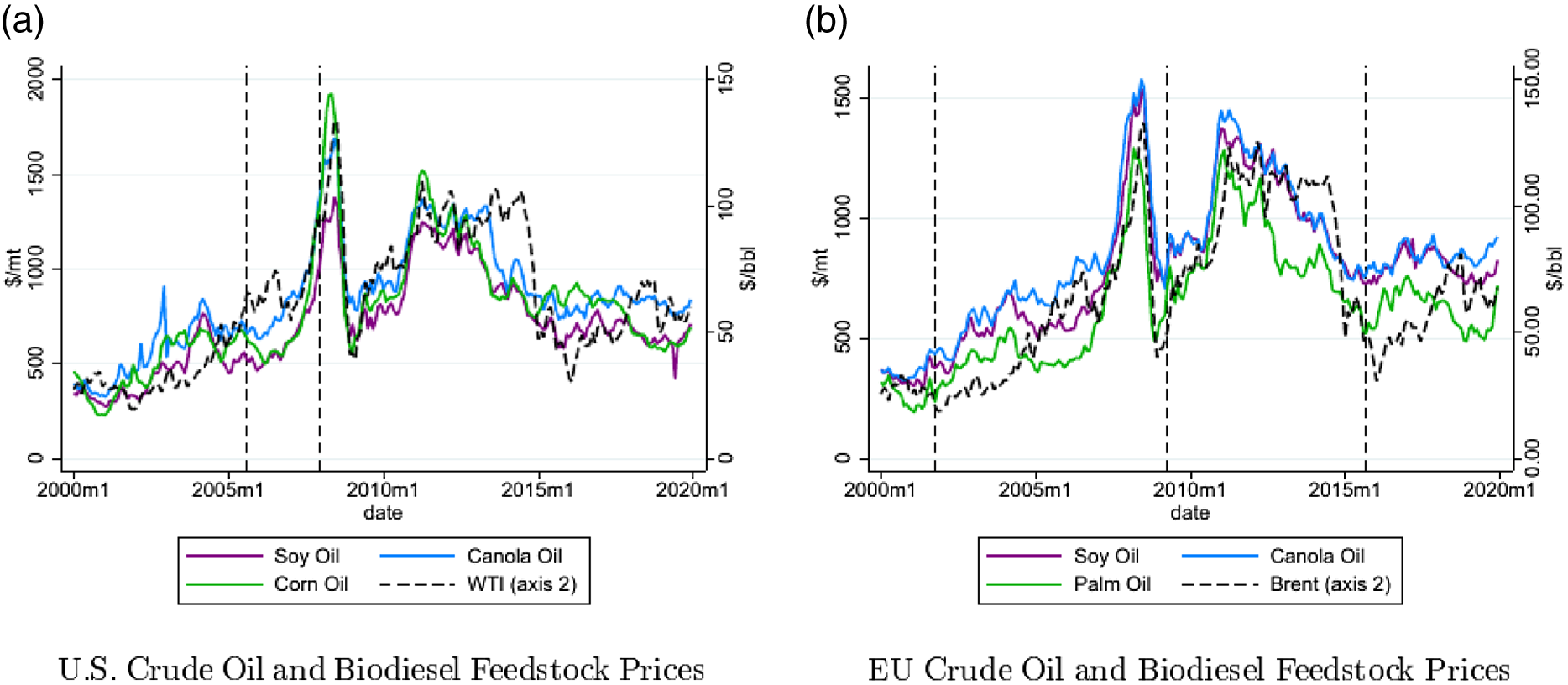
Figure 3. Biodiesel feedstock and crude oil prices. US soy oil and corn oil price data (panel a) are obtained from the USDA, Foreign Agriculture Service, “Oilseeds: World Markets & Trade” report. US soy oil prices for Decatur (average wholesale tank price), and corn oil prices are FOB, Chicago. US canola oil prices (panel a) are a Midwest-average price obtained from the USDA ERS “Oil Crops Yearbook”. WTI crude prices (panel a) are FOB Cushing, Oklahoma spot prices obtained from the US Department of Energy, Energy Information Administration (EIA). EU soy oil and canola oil prices (FOB Rotterdam) in panel (b) are obtained from the USDA FAS. Palm oil prices (panel b) used in the EU analysis are FOB Malaysia (also obtained from USDA FAS). Brent crude oil prices (panel b) are FOB spot prices obtained from Thomson Reuters. Vertical dashed lines in the figure represent the dates of major biofuels legislation.
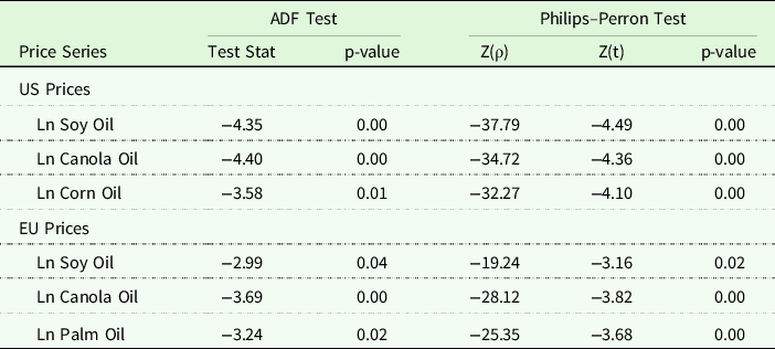
Table 1 provides the results for the augmented Dickey–Fuller and Philips–Perron tests for nonstationarity in the biodiesel feedstock and crude oil price data, estimated in natural logarithmic form and using a two-period lag specification. As shown in the Table, we fail to reject a unit root for all price levels. We account for this in our econometric specification below.
Table 1. Tests for nonstationarity

Note: Table presents results for tests for nonstationarity in the biodiesel feedstock and crude oil price data, estimated in natural logarithmic form. ADF tests use a two-period lag specification.
Econometric model
The long-run equilibrium relationship – if one exists – between the price for a given biodiesel feedstock and the price for crude oil, can be expressed as
 $$P_t^f = {\mu ^f} + {\theta ^f}P_t^{crude}$$
where variable $P_t^f$
describes the price at a given time
$P_t^f$
describes the price at a given time $t$
for the specific biodiesel feedstock
$t$
for the specific biodiesel feedstock $f$
. For our purposes, we consider
$f$
. For our purposes, we consider $f \in $
{soy oil, canola oil, corn oil} for the US models and
$f \in $
{soy oil, canola oil, corn oil} for the US models and $f \in $
{soy oil, canola oil, palm oil} for the EU models. We define the contemporaneous price of crude oil, variable
$f \in $
{soy oil, canola oil, palm oil} for the EU models. We define the contemporaneous price of crude oil, variable $P_t^{crude}$
on the right-hand side, alternatively as the WTI price for the US price relationships and the Brent price for the EU relationships.
$P_t^{crude}$
on the right-hand side, alternatively as the WTI price for the US price relationships and the Brent price for the EU relationships.
Our purpose is to assess the impacts of major biofuels legislation and global crude oil supply expansion on these cointegrating relationships. To do so, we estimate the following models:
 \begin{align}P_t^f &= \alpha _0^f + \beta _0^fP_t^{crude} + \mathop \sum \nolimits_{n = 1}^N \left( {\alpha _n^fPolicy_t^n + \beta _n^fPolicy_t^nP_t^{crude}} \right)\\
&\quad + \left( {\alpha _G^fG_t^{crude} + \beta _G^fG_t^{crude}P_t^{crude}} \right) + \varepsilon _t^f\end{align}
\begin{align}P_t^f &= \alpha _0^f + \beta _0^fP_t^{crude} + \mathop \sum \nolimits_{n = 1}^N \left( {\alpha _n^fPolicy_t^n + \beta _n^fPolicy_t^nP_t^{crude}} \right)\\
&\quad + \left( {\alpha _G^fG_t^{crude} + \beta _G^fG_t^{crude}P_t^{crude}} \right) + \varepsilon _t^f\end{align}
Parameters $\alpha _0^f$
and
$\alpha _0^f$
and $\beta _0^f$
describe the baseline cointegrating relationship. We allow this baseline cointegrating relationship to evolve in two ways:
$\beta _0^f$
describe the baseline cointegrating relationship. We allow this baseline cointegrating relationship to evolve in two ways:
Policy-induced regime change: First, we allow the promulgation of major biofuels legislation in the US and EU to induce change in the intercept and slope terms characterizing the long-run equilibrium relationship. This structural change process is described by the second set of terms in equation (2). Variables $Policy_t^n$
are dummy variables that describe a set of policies
$Policy_t^n$
are dummy variables that describe a set of policies $n \in $
{1, …, N}. The dummy variables take value one in time periods on and after the introduction of a given policy
$n \in $
{1, …, N}. The dummy variables take value one in time periods on and after the introduction of a given policy $n$
and are equal to zero beforehand. The post-policy cointegrating relationship is described by the sum of the baseline parameters and the policy shift parameters.
$n$
and are equal to zero beforehand. The post-policy cointegrating relationship is described by the sum of the baseline parameters and the policy shift parameters.
As described above in the Background section, the two major biofuels policy changes in the US include the enactment of the Energy Policy Act in August 2005 and the Energy Independence and Security Act in December 2007. Thus, in the US models, we include dummies $Polic{y^1}$
(equal to one for periods on and after August 2005) and
$Polic{y^1}$
(equal to one for periods on and after August 2005) and $Polic{y^2}$
(equal to one for periods on and after December 2007) to represent these policy changes. The EU has three major pieces of biofuels legislation. The first – and most meaningful piece of legislation – was the Biofuels Directive of 2001, which was enacted in October 2001. Subsequently, the EU adopted the Renewable Energy Directive in April 2009. Finally, in October 2015, the EU adopted the Indirect Land Use Change Directive, which reduced the share of land that could be devoted to biofuels feedstocks. Because our sample runs from year 2000, we have a limited number of observations prior to the enactment of the Biofuels Directive of 2001. Accordingly, for the EU models, we set the sample start date as October 2001, where the “baseline” parameters are interpreted as in light of the Directive. As in the US specification, we include two policy dummies
$Polic{y^2}$
(equal to one for periods on and after December 2007) to represent these policy changes. The EU has three major pieces of biofuels legislation. The first – and most meaningful piece of legislation – was the Biofuels Directive of 2001, which was enacted in October 2001. Subsequently, the EU adopted the Renewable Energy Directive in April 2009. Finally, in October 2015, the EU adopted the Indirect Land Use Change Directive, which reduced the share of land that could be devoted to biofuels feedstocks. Because our sample runs from year 2000, we have a limited number of observations prior to the enactment of the Biofuels Directive of 2001. Accordingly, for the EU models, we set the sample start date as October 2001, where the “baseline” parameters are interpreted as in light of the Directive. As in the US specification, we include two policy dummies $Polic{y^1}$
(equal to one for periods on and after April 2009) and
$Polic{y^1}$
(equal to one for periods on and after April 2009) and $Polic{y^2}$
(equal to one for periods on and after October 2015) to represent the subsequent policy changes.
$Polic{y^2}$
(equal to one for periods on and after October 2015) to represent the subsequent policy changes.
Oil expansion shifters: Second, we allow the cointegrating relationship between biodiesel feedstock and crude oil prices to shift gradually over time due to expansions (or contractions) in the global oil supply. We model these smooth shifts using the third set of terms in equation (2). Variable $G_t^{crude}$
represents annual global crude oil production values. This variable enters the model independently as an intercept shifter and via the interaction with the crude oil price as slope shifter. Annual observations of
$G_t^{crude}$
represents annual global crude oil production values. This variable enters the model independently as an intercept shifter and via the interaction with the crude oil price as slope shifter. Annual observations of $G_t^{crude}\;$
are matched with our monthly price dataset by calendar year. The annual time step reflects the fact that these shifts in the cointegration process occur gradually over time, rather than based on contemporaneous monthly production values.
$G_t^{crude}\;$
are matched with our monthly price dataset by calendar year. The annual time step reflects the fact that these shifts in the cointegration process occur gradually over time, rather than based on contemporaneous monthly production values.
Residual-based tests for cointegration: To assess cointegration across regimes, we report results for augmented Dickey-Fuller (ADF) and Phillips–Perron for stationarity of the residual term from equation (2) (Dickey and Fuller, Reference Dickey and Fuller1979; Phillips and Perron, Reference Phillips and Perron1988). After estimation, we also conduct Wald tests to assess the statistical significance of the postchange long-run equilibrium parameters.
Results
Figures 4 and 5 report – for the US and EU, respectively – the estimated cointegrating relationship between biodiesel feedstock and crude oil prices obtained from equation (2). The figures further show the impacts of major biofuels legislation and global crude oil supply expansion on these cointegrating relationships.Footnote
2
Panels (a), (b), and (c) of the figures plot the change in the cointegration coefficient attributable to each policy regime (Regime 1 = $\hat \beta _0^f$
, Regime 2 =
$\hat \beta _0^f$
, Regime 2 = $\hat \beta _0^f + \hat \beta _1^f$
, and Regime 3 =
$\hat \beta _0^f + \hat \beta _1^f$
, and Regime 3 = $\hat \beta _0^f + \hat \beta _1^f + \hat \beta _2^f$
). Panels (d), (e), and (f) of the figures plot the shift in the cointegration coefficient attributable to global oil expansion
$\hat \beta _0^f + \hat \beta _1^f + \hat \beta _2^f$
). Panels (d), (e), and (f) of the figures plot the shift in the cointegration coefficient attributable to global oil expansion $\big( {\hat \beta _G^f \times {G^{crude}}} \big)$
over the relevant range of global oil production. Panels (g), (h), and (i) plot the evolution in the cointegration coefficient (
$\big( {\hat \beta _G^f \times {G^{crude}}} \big)$
over the relevant range of global oil production. Panels (g), (h), and (i) plot the evolution in the cointegration coefficient ( $\hat \beta _0^f + \hat \beta _1^f \times Policy_t^1 + \hat \beta _2^f \times Policy_t^2 + \hat \beta _G^f \times {G^{crude}}$
) for each cointegrating relationship over time.Footnote
3
$\hat \beta _0^f + \hat \beta _1^f \times Policy_t^1 + \hat \beta _2^f \times Policy_t^2 + \hat \beta _G^f \times {G^{crude}}$
) for each cointegrating relationship over time.Footnote
3
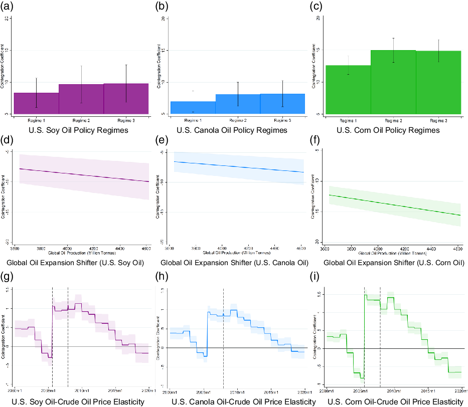
Figure 4. US crude oil-to-biodiesel-feedstock cointegration relationships. Panels (a), (b), and (c) of the figure plot the change in the cointegration coefficient attributable to each policy regime (Regime 1 = $\hat \beta _0^f$
, Regime 2 =
$\hat \beta _0^f$
, Regime 2 = $\hat \beta _0^f + \hat \beta _1^f$
, and Regime 3 =
$\hat \beta _0^f + \hat \beta _1^f$
, and Regime 3 = $\hat \beta _0^f + \hat \beta _1^f + \hat \beta _2^f$
) for US soy oil, canola oil, and corn oil models, respectively. Panels (d), (e), and (f) of the figures plot the shift in the cointegration coefficient attributable to global oil expansion
$\hat \beta _0^f + \hat \beta _1^f + \hat \beta _2^f$
) for US soy oil, canola oil, and corn oil models, respectively. Panels (d), (e), and (f) of the figures plot the shift in the cointegration coefficient attributable to global oil expansion $\big( {\hat \beta _G^f \times {G^{crude}}} \big)$
over the relevant range of global oil production. Panels (g), (h), and (i) plot the evolution in the cointegration coefficient (
$\big( {\hat \beta _G^f \times {G^{crude}}} \big)$
over the relevant range of global oil production. Panels (g), (h), and (i) plot the evolution in the cointegration coefficient ( $\hat \beta _0^f + \hat \beta _1^f \times Policy_t^1 + \hat \beta _2^f \times Policy_t^2 + \hat \beta _G^f \times {G^{crude}}$
) for each cointegrating relationship over time. Confidence intervals in panel (c) are constructed using the Bayesian Bootstrap method with 1,000 draws from the posterior distributions of parameters
$\hat \beta _0^f + \hat \beta _1^f \times Policy_t^1 + \hat \beta _2^f \times Policy_t^2 + \hat \beta _G^f \times {G^{crude}}$
) for each cointegrating relationship over time. Confidence intervals in panel (c) are constructed using the Bayesian Bootstrap method with 1,000 draws from the posterior distributions of parameters $\hat \beta _0^f$
,
$\hat \beta _0^f$
, $\hat \beta _n^f$
, and
$\hat \beta _n^f$
, and $\hat \beta _G^f$
from equation (2).
$\hat \beta _G^f$
from equation (2).
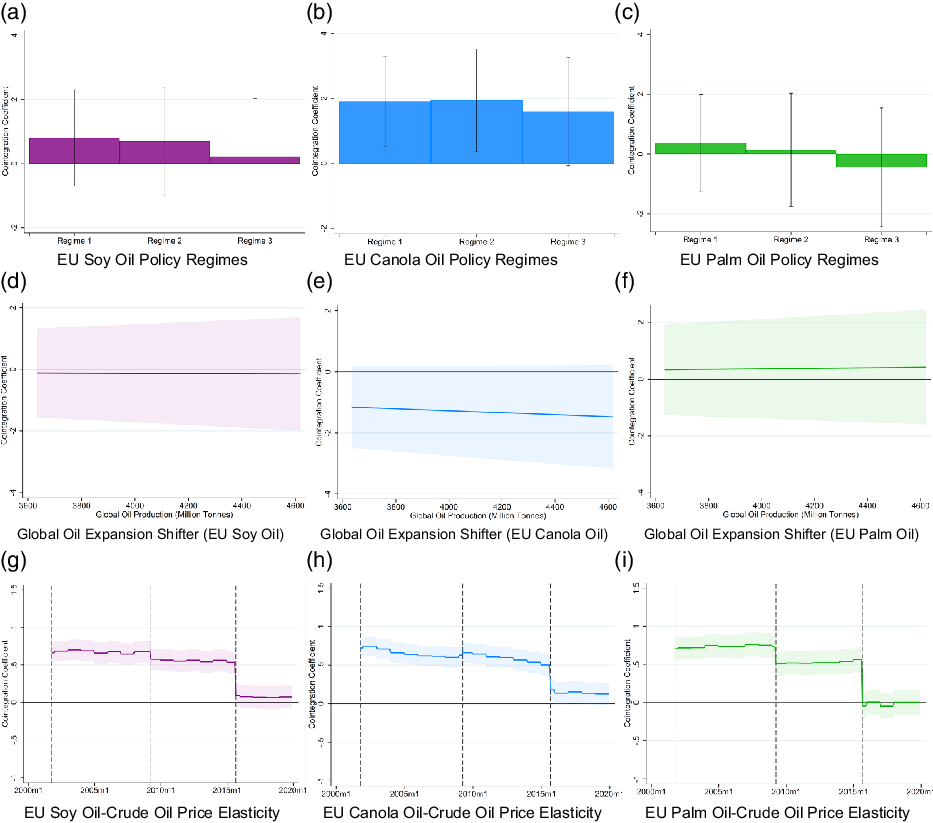
Figure 5. EU crude oil-to-biodiesel-feedstock cointegration relationships. Panels (a), (b), and (c) of the Figure plot the change in the cointegration coefficient attributable to each policy regime (Regime 1 = $\hat \beta _0^f$
, Regime 2 =
$\hat \beta _0^f$
, Regime 2 = $\hat \beta _0^f + \hat \beta _1^f$
, and Regime 3 =
$\hat \beta _0^f + \hat \beta _1^f$
, and Regime 3 = $\hat \beta _0^f + \hat \beta _1^f + \hat \beta _2^f$
) for EU soy oil, canola oil, and palm oil models, respectively. Panels (d), (e), and (f) of the Figures plot the shift in the cointegration coefficient attributable to global oil expansion
$\hat \beta _0^f + \hat \beta _1^f + \hat \beta _2^f$
) for EU soy oil, canola oil, and palm oil models, respectively. Panels (d), (e), and (f) of the Figures plot the shift in the cointegration coefficient attributable to global oil expansion $\big( {\hat \beta _G^f \times {G^{crude}}} \big)$
over the relevant range of global oil production. Panels (g), (h), and (i) plot the evolution in the cointegration coefficient (
$\big( {\hat \beta _G^f \times {G^{crude}}} \big)$
over the relevant range of global oil production. Panels (g), (h), and (i) plot the evolution in the cointegration coefficient ( $\hat \beta _0^f + \hat \beta _1^f \times Policy_t^1 + \hat \beta _2^f \times Policy_t^2 + \hat \beta _G^f \times {G^{crude}}$
) for each cointegrating relationship over time. Confidence intervals in panel (c) are constructed using the Bayesian Bootstrap method with 1,000 draws from the posterior distributions of parameters
$\hat \beta _0^f + \hat \beta _1^f \times Policy_t^1 + \hat \beta _2^f \times Policy_t^2 + \hat \beta _G^f \times {G^{crude}}$
) for each cointegrating relationship over time. Confidence intervals in panel (c) are constructed using the Bayesian Bootstrap method with 1,000 draws from the posterior distributions of parameters $\hat \beta _0^f$
,
$\hat \beta _0^f$
, $\hat \beta _n^f$
, and
$\hat \beta _n^f$
, and $\hat \beta _G^f$
from equation (2).
$\hat \beta _G^f$
from equation (2).
Referring first to panels (a), (b), and (c) of Figure 4, we examine the impacts of US regulatory change, independent from changes in global crude oil production levels. As shown in the figure, even prior to the enactment of the US Energy Policy Act in August, biodiesel feedstock prices responded positively to long-run shocks to WTI crude oil prices. Each of these responses was statistically significant at the 1% level. These results are plotted as “Regime 1” in panel (c) of the figure. Comparing among US biodiesel feedstocks in Regime 1, our partial elasticity estimates suggest that – before accounting for changes in oil production levels – corn oil prices were most responsive to crude oil price shocks: a 1% increase in the price of crude oil corresponded to a 12.6% increase in the price of corn oil. The comparable long-run partial elasticity for soy oil (panel a) and canola oil (panel b), respectively, were 8.3 and 6.97, respectively.
The promulgation of the 2005 Energy policy Act (shown as “Regime 2” in panels (a), (b), and (c) of Figure 4 increased the responsiveness of prices for each of the biodiesel feedstocks (statistically significant at the 1% level). The corn oil price partial elasticity response in panel (c) increased from 12.6 to 15.0. Soy oil in panel (a) and canola oil in panel (c) increased from 8.3 to 9.7 and from 6.97 to 8.1. This increase in biodiesel feedstock prices to crude oil price shocks is as expected (see Figure 2). However, Regime 3, under the Energy Independence & Security Act, which increased US biodiesel production with RFS2, does not appear to have generated a meaningful response beyond that from Regime 2 (the Energy Policy Act). This suggests that the effects of biodiesel incentives were already “baked into” the market by this time, and additional expansion of the industry did not substantially alter market equilibrium.
Turning to Panels (d), (e), and (f) of Figure 4, expansion of the global crude oil supply leads to a reduction in the biodiesel feedstock price response. This result is statistically significant at the 1% level for all feedstocks, and – as with the baseline responses – the corn oil price response is most sensitive to changes in global crude oil production levels. According to this partial elasticity, a 1% increase in annual crude oil production reduces the corn oil price responses by an estimated 0.3% (panel f) and 0.2% for soy oil (panel d) and canola oil (panel e) prices.
Turning to panels (g), (h), and (i) of Figure 4, we see that these two factors have changed substantially over time the total response in biodiesel feedstock prices resulting from a shock to crude oil prices. After accounting for subsequent policy regime changes and global oil production levels, we see that – on average in the early 2000s – a 1% increase in the crude oil price corresponded to a 0.29% total increase in the soy oil price (panel g), a 0.25% increase in the canola oil price (panel h), and a 0.5% increase in the corn oil price (panel i). All of these responses were statistically significant at the 1% level. After the enactment of the 2005 Energy Policy Act, average total elasticity responses increased to 0.96% for soy oil (panel g), 0.87% for canola oil (panel h), and 1.38% for corn oil (panel i). All of these total elasticities are statistically significant at the 1% level. By January 2015, we estimate that the responsiveness fell to 0.18% for soy oil (panel g), 0.16% for canola oil (panel h), and −0.10% (statistically indistinguishable from zero) for corn oil (panel i). This suggests that – in the modern biodiesel era – the expansion in the global supply of crude oil, due predominantly to shale oil technology, has overshadowed the effects of US biodiesel incentives and blending mandates instituted under the Energy Policy Act and the Energy Independence and Security Act.
These findings also reconcile the disconnect in the previous literature. In the early periods, we find a low degree of cointegration between biodiesel feedstock and crude oil prices consistent with Yu, Bessler, and Fuller (Reference Yu, Bessler and Fuller2006) and Zhang et al. (Reference Zhang, Lohr, Escalante and Wetzstein2010). In the periods surrounding the food price spike, we see a high degree of cointegration between biodiesel feedstock and crude oil prices, consistent with Abdel and Arshad (Reference Abdel and Arshad2008), Ghaith and Awad (Reference Ghaith and Awad2011), and Esmaeili and Shokoohi (Reference Esmaeili and Shokoohi2011).
Comparing the relative responsiveness of the various biodiesel feedstocks, the fact that the largest crude oil price response during the food price spike period observed for corn oil is consistent with the fact that corn production is linked with both ethanol and biodiesel production. The fact that soy oil prices are slightly more responsive to crude oil prices is also consistent with the findings from Schaefer et al. (Reference Schaefer, Myers, Johnson, Helmar and Radich2021) with respect to the price premiums for canola oil relative to soy oil over the past two decades.
EU cointegration coefficients, shown in Figure 5, differ in important ways from those for the US. Referring to panels (a), (b), and (c), in contrast to the US prices, Regime 1 biodiesel feedstock prices were highly responsive to crude oil price shocks. This is consistent with policy differences across the two nations. Recall that the US did not adopt meaningful biofuels legislation until 2005, whereas the EU adopted the Biofuels Directive in 2001. Also in contrast to the US, in the EU, canola prices are most responsive to crude oil price shocks at baseline. The canola price elasticity is 1.91 (panel b), compared to 0.80 and 0.38 for soy oil (panel a) and palm oil (panel c). The subsequent Renewable Fuels Directive (Regime 2) did not generate meaningful changes to biodiesel feedstock–crude oil price relationships. This is consistent with subsequent US legislation, and suggests that biodiesel incentives were priced into the market by that time.
The ILUC Directive, which reduced the land area devoted to biodiesel feedstocks in the EU, generated a substantial reduction in the feedstock price responsiveness. The palm oil price response fell by 0.58 (panel c), the soy oil price (panel a) response fell by 0.47, and the canola oil price (panel b) response fell by 0.35 (each statistically significant at the 1% level). As shown in panels (d), (e), and (f) of Figure 5, we do not observe a statistically significant change in biodiesel feedstock price responsiveness as a result of changes to the global crude oil supply.
In panels (g), (h), and (i) of Figure 5, we see that – on net – EU feedstock prices were more responsive to crude oil prices than those in the US (shown in Figure 4) prior to 2005. A 1% increase in the crude oil price resulted in a 0.70% increase in EU canola oil prices (compared to 0.25% for US canola oil prices) and a 0.67% increase in EU soy oil prices (compared to 0.29% for US soy oil prices). In the wake of the ILUC Directive, these EU price responses fell to an average of 0.14% for canola oil, 0.07% for soy oil, and −0.02% (statistically indistinguishable from zero) for palm oil.
After deriving the total elasticity estimates, we formally test for cointegration using ADF and Phillips–Perron residual-based tests.Footnote 4 These results are reported in Table 2. As shown in Table 2, according to both tests, we reject at the 5% level the null hypothesis that the residuals follow unit root processes for all models. Accordingly, we can conclude the biodiesel feedstock prices are cointegrated with crude oil prices over the sample period.
Table 2. Residual-based cointegration tests
Model robustness
An implicit assumption in the construction of equation (2) is that the impact of major biofuels legislation on biodiesel feedstock–crude oil equilibrium price relationships is contemporaneous with their promulgation and implementation. However, it is not clear a priori when these policy treatments occur. For example, it is logical that some of the impacts of major legislative actions were anticipated prior to implementation and therefore may have at least some impact prior to enactment. It is also possible that some adjustment to legislative changes may be delayed due to adjustment costs and rigidities. We assess the sensitivity of the results in the Results section by reestimating the models described in equation (2), randomly drawing a possible “effective” start date for each policy regime change variable ( $Policy_t^n$
) from the window of time beginning 6 months before the enactment of the relevant legislation and ending 6 months after enactment.Footnote
5
As in equation (2), these dummy variables are then defined to take value one in time periods on or after the “effective” start date of the given policy and equal to zero beforehand. For each biodiesel feedstock, we repeat this re-estimation process 100 times to get a distribution of point estimates for our coefficients.
$Policy_t^n$
) from the window of time beginning 6 months before the enactment of the relevant legislation and ending 6 months after enactment.Footnote
5
As in equation (2), these dummy variables are then defined to take value one in time periods on or after the “effective” start date of the given policy and equal to zero beforehand. For each biodiesel feedstock, we repeat this re-estimation process 100 times to get a distribution of point estimates for our coefficients.
Figure 6 reports the results of this sensitivity analysis. In each panel of the figure, the left and right sides of each box represent the lower and upper quartiles for the coefficients obtained from re-estimating equation (2) with 100 draws of the policy regime change variables. The horizontal line that splits each box is the median coefficient estimate. The whiskers depict the range from the lower quartile to the upper quartile. The red scatter dots and red vertical lines depict the corresponding point estimate and 95% confidence interval for the main model described in the Results section.

Figure 6. Coefficient estimates from alternative policy regime change timing. In each panel, the left and right sides of each box represent the lower and upper quartiles for the coefficients obtained from re-estimating equation (2) with 100 draws of the policy regime change variables. The horizontal line that splits each box is the median coefficient estimate. The whiskers depict the range from the lower quartile to the upper quartile. The red scatter dots and red vertical lines depict the corresponding point estimate and 95% confidence interval for the main model described in the Results section.
As shown in Figure 6, the results of the sensitivity analysis are broadly consistent with the point estimates from our baseline model. Specifically, in both the EU and US models, the coefficient estimates for $\beta _0^f$
and
$\beta _0^f$
and $\beta _G^f$
appear insensitive to our assumptions regarding the timing of policy impacts. Impact estimates for the Energy Independence and Security Act appear most sensitive to our timing assumptions. Because these effects are statistically indistinguishable from zero in our baseline model, we do not find this concerning.
$\beta _G^f$
appear insensitive to our assumptions regarding the timing of policy impacts. Impact estimates for the Energy Independence and Security Act appear most sensitive to our timing assumptions. Because these effects are statistically indistinguishable from zero in our baseline model, we do not find this concerning.
Conclusion
In this paper, we seek to disentangle the effects of biodiesel incentives and shale oil expansion on the long-run equilibrium price relationship among biodiesel feedstocks and crude oil in the US and EU. We find that the promulgation of the 2005 Energy Policy Act in the US substantially increased the responsiveness of soy oil, canola oil, and corn oil prices to crude oil price shocks. However, in recent years, expansion in the global supply of crude oil has overshadowed the effects of US biodiesel incentives and blending mandates. In the EU, the Indirect Land Use Change (ILUC) Directive of 2015 substantially reduced the responsiveness of biodiesel feedstock prices to crude oil price shocks.
Of course, as with any research, our paper is not without qualifications. We note that the equilibrium relationships measured correspond to prices at specific geographic locations. While these geographic locations are well-chosen to represent a primary production source for the products of the study, prices for the same products in different locales may yield different empirical results. Moreover, it is possible that oil prices may matter more in determining biodiesel feedstock prices in periods of high price volatility than in low price volatility. While there is a literature on the relationship between oil price volatility affects agricultural prices (Arnade and Hoffman, Reference Arnade and Hoffman2015; McPhail et al., Reference McPhail, Du and Muhammad2012; Wang and McPhail, Reference Wang and McPhail2014), our results do not directly speak to this issue.
Finally, recent months have seen major disruptions to commodity markets resulting from restrictions on local and international movements to slow the COVID-19 pandemic and negative shocks to the economy caused by the pandemic. These disruptions may cause a breakdown in the equilibrium price relationships among biodiesel feedstock and crude oil prices, particularly considering the slowdown in biofuels production and use. The extent to which these COVID-19 shocks are transitory or more permanent remains to be seen.
Data availability statement
All data and programs necessary to replicate the analyses and results in this manuscript are available from the authors upon request.
Funding statement
This work was supported by the United States Department of Agriculture under award 58-0111-19-006. The findings and conclusions in this publication are those of the author(s) and should not be construed to represent any official USDA or US Government determination or policy.
Conflicts of interest
The authors report no conflicting interests relevant to this work.
Ethical standards
This project did not involve human subjects research.
Appendix
Table A1. US crude oil–biodiesel feedstock cointegration relationships
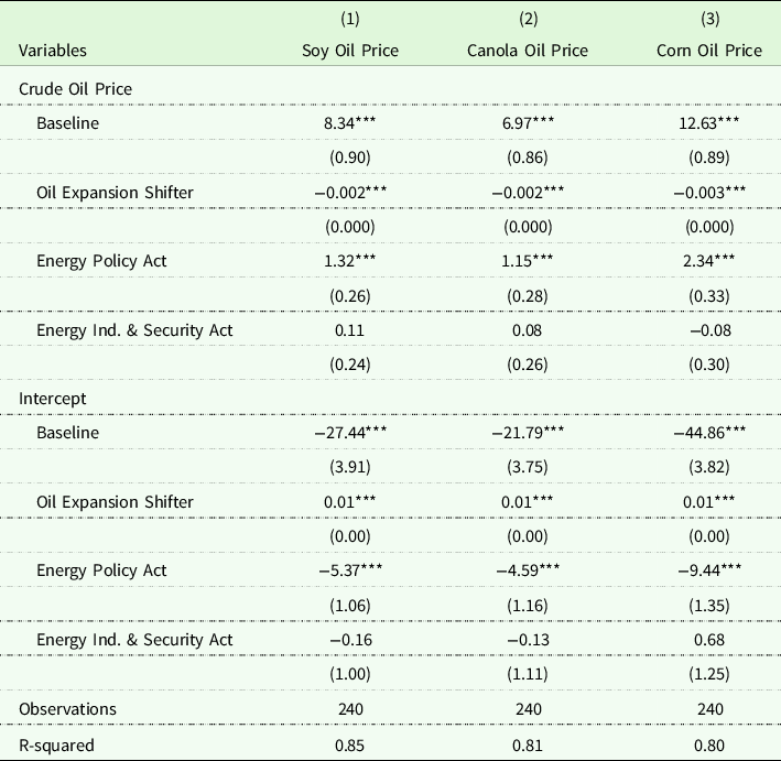
Robust standard errors in parentheses.
***p < 0.01, **p < 0.05, *p < 0.1.
Table A2. EU crude oil–biodiesel feedstock cointegration relationships
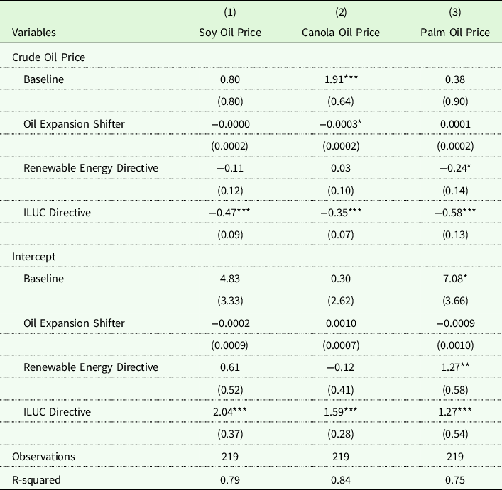
Standard errors in parentheses are bootstrapped according to Mooney and Duval (Reference Mooney and Duval1993), with 50 replications.
***p < 0.01, **p < 0.05, *p < 0.1.

Figure A1. Crude oil-to-biodiesel feedstock cointegration model residuals. Figure plots residuals obtained from estimating equation (2). Vertical dashed lines in the figure represent the dates of major biofuels legislation.


 Open access