


Introduction
The work study is a widely used approach for analyzing how tasks are carried out in a company and recommending steps to enhance efficiency. Frederick Winslow Taylor (1856–1915) emphasized the need to follow the three basic principles to maximize productivity: (i) “a defined task, determined by the definition of the job leading to the best operation sequence,” (ii) “a definite time, established by stopwatch time study or estimated from standard data,” and (iii) “a definite method developed by detailed analysis and recorded in the instruction charts.” Taylor's main contribution to work study is therefore the timing of each action and finding the “one optimum method” to do a task. All of these concepts are represented in his book “Shop Management” (Taylor, Reference Taylor1911).
The two core concepts in work study are motion study and work measurement. Motion study focuses on the effectiveness of the work and work study provides the standard time that is required for different purposes. The type of applied work measurement technique can vary according to the work specifications and structure that will be measured. Work measurement is the application of the predefined techniques by a qualified worker with a required measurement of time to validate work with a predetermined definition (standardized) and performance level.
The work study is not a single technique but a definition that consists of a group of techniques that are used to measure the work (Niebel and Freivalds, Reference Niebel and Freivalds2003).
Companies today have a tremendous need to monitor the standard times for the items they manufacture (Freivalds et al., Reference Freivalds, Konz, Yurgec and Goldberg2000). Without precise standard time, it is extremely challenging to design manufacturing schedules, short- and long-term estimates, capacity planning, pricing, and other technical and administrative tasks in a firm (Eraslan, Reference Eraslan2009). Because determining the standard time is challenging, extra work measurement methodologies, such as time study, are required in addition to direct measurement techniques (Dağdeviren et al., Reference Dağdeviren, Eraslan and Çelebi2011). It is obvious that not all firms can determine the standard time for each product or semi-product using indirect labor measuring methods. However, for some products, when the time study is expensive or not practicable, they are extremely useful approaches. Unfortunately, in most situations, direct or indirect work measurement techniques such as “time study,” “activity sampling,” “standard data synthesis,” “analytical estimation,” “comparison,” “prediction,” and “elementary motion standards” are inadequate to ensure the precise standard time (Atalay et al., Reference Atalay, Eraslan and Cinar2015). As a result, new and effective techniques for dealing with this problem are required. The primary goal of this study is to apply machine learning algorithms for estimating the standard time based on various parameters including the number of products, the number of welding operations, product's surface area factor, difficulty/working environment factor, and the number of metal forming processes.
The rest of this study is organized as follows. The literature review is presented in the part after that, Section “Background”. Section “Material and methodology” introduces machine learning methods and presents a study design. Comparing the results of the selected machine learning techniques is covered in Section “Results and discussion”, and Section “Conclusions” examines the findings and makes recommendations for further research.
Background
To increase the efficient use of resources and set performance criteria for the selected activities, work study is the systematic assessment of activity-conduct procedures (Kanawaty, Reference Kanawaty1992). Some of the recent studies on work study have been conducted by several authors. For instance, Moktadir et al. (Reference Moktadir, Ahmed, Zohra and Sultana2017) used the work study approach to enhance productivity in the leather goods business. They demonstrated that reducing work content and balancing lines improved productivity. In order to determine the average and standard times for each task included in the manual palm oil harvesting process, Saibani et al. (Reference Saibani, Muhamed, Maliami and Ahmad2015) observed two harvesters. Khan and Jha (Reference Khan and Jha2017) evaluated a production line of a high-deck body and performed a time study to determine the standard time for each process.
Suyono (Reference Suyono2021) recently estimated the cycle time, normal time, and standard time for each work process done by employees while accounting for the adjustment factor and the allowance factor to differentiate the types of labor. Ahmed et al. (Reference Ahmed, Islam and Kibria2018) predicted the standard time based on an effective layout model of a shirt manufacturing company. The authors investigated different types of machines such as cutting machine and sewing machine. Rosa et al. (Reference Rosa, Silva, Ferreira, Pereira and Gouveia2018) improved an assembly line's production process by removing non-value-adding tasks. Similarly, Rosa et al. (Reference Rosa, Silva, Ferreira and Campilho2017a, Reference Rosa, Silva and Ferreira2017b) considerably improved the manufacture of control cables used in car vehicles to operate doors and windows. SMED (single minute exchange of die) approaches were used in various jobs, as well as value stream mapping (VSM) analysis and standard work principles. Significant productivity increases were made in a product with a low added value and a labor-intensive assembly process. An electronic component company enhanced the efficiency of their assembly line by 10% using VSM and lean line design (Correia et al., Reference Correia, Silva, Gouveia, Pereira and Ferreira2018). Various levels of production standard time were examined by Nurhayati et al. (Reference Nurhayati, Zawiah and Mahidzal2016) to determine the relationship between work productivity and acute reactions. They concluded that their findings are useful for assessing workers’ current work productivity and serving as a reference for future work productivity planning to reduce the risk of developing work-related musculoskeletal disorders (WMSDs). Eraslan (Reference Eraslan2009) proposed the artificial neural network (ANN)-based approach for standard time estimation in the molding sector. The proposed approach, according to the author, might be used with accuracy in comparable procedures. Similarly, for standard time estimate in particular production systems, Atalay et al. (Reference Atalay, Eraslan and Cinar2015) used fuzzy linear regression analysis with quadratic programming.
This research is a considerable expansion of the study undertaken by Dağdeviren et al. (Reference Dağdeviren, Eraslan and Çelebi2011), in which the dataset was used to develop and evaluate ANNs. In this study, more data were collected to build and test 13 machine learning algorithms for estimating the standard time. These algorithms include linear (“multiple linear regression, ridge regression, lasso regression, and elastic net regression”) and nonlinear models [“k-nearest neighbors, random forests, artificial neural network, support vector regression, classification and regression tree (CART), gradient boosting machines (GBM), extreme gradient boosting (XGBoost), light gradient boosting machine (LightGBM), and categorical boosting (CatBoost)”].
Despite extensive research on work study applications, there is a dearth of data on how to model the relationship between components of the manufacturing environment and standard time. The literature indicates that no research has been performed on the use of any machine learning technique specifically for this objective in order to ascertain the extent to which production environment features contribute to the computation of the standard time. This fact has served as the basis for the current study. Thus, the current work will contribute to the domain of work study and ergonomics.
Material and methodology
Work measurement techniques
It is possible to define the work measurement techniques as indirect techniques where direct observation is required (time study, group timing technique, work sampling) and as direct techniques where direct observation is not required (predetermined motion-time systems, standard data and formulation, comparison and prediction methods) (Niebel and Freivalds, Reference Niebel and Freivalds2003). The most common ones are briefly explained below:
(i) A time study (TS) captures the process time and levels of a planned work under specific conditions. The obtained data are evaluated and used to determine how long it will take to complete the task at a set process speed (Niebel and Freivalds, Reference Niebel and Freivalds2003). Time measurements, especially by using work technique, method and conditions of the work systems, consist of proportionality quantities, factors, performance levels, and evaluation of real time for each flow section. The specified flow sections’ foresight time is determined using the evaluations of this time. Unfortunately, time study is cost ineffective and can be used only under certain situations. Furthermore, it depends on the expertise of the individual conducting the time study.
(ii) Work sampling (WS) is the determination of the frequency of the occurrence of the flow types that are previously determined for one or more similar work systems by using randomness and short time observations. The state of the worker or the machine that is randomly observed is recorded and the free time percentages of the worker or machine, even a workshop, are determined after many sufficient observations. WS is based on probability fundamentals, for the assumption that the sample group will represent the mass similarly done in similar statistical studies. As the sample size is increased, the reliability of the measurement will increase. There are some advantages of WS such that it does not require any experience and can be performed using less effort compared with TS. However, some of the disadvantages of this method are the difficulties in observing separate machines, not providing a performance evaluation, informing groups rather than individual people and problems based on non-clear observations of some flow sections (Niebel and Freivalds, Reference Niebel and Freivalds2003).
(iii) Predetermined motion-time system (MTM) is an indirect work study technique. Motion-time systems, also named as synthetic time systems, are used to determine the time needed for a related work by means of using predetermined time standards for some motions without a direct observation and measurement. It is, however, only applicable to hand-made processes (Niebel and Freivalds, Reference Niebel and Freivalds2003).
(iv) Time study in individual and discrete serial manufacturing, small-sized establishments, re-work activities, or producing a new product in manufacturing lines is very expensive or not possible. For this reason, the time study in these fields is mostly determined by a comparison and prediction method (CPM). The flow time, which is evaluated by the reference time, is deduced by comparing it with a predetermined similar product's flow time. This method is capable of obtaining data that can be used under some special circumstances if there exists sufficient experience, provided documents and the correct application of the method. This method requires forecasts and measurements are affected mostly by the personal opinions of the one who performs the time study (Niebel and Freivalds, Reference Niebel and Freivalds2003).
(v) Standard data and formulation method (SDF) is based on the formulation that the work time is calculated using the previously completed time studies and assume that the factors affecting the time are declared as variables. Regression analysis is one of these methods. The most significant disadvantages of this method are the impossibility of deriving a formulation expressing the behavior of all systems and the condition of ineffectiveness of a mathematical function that effect time.
Direct or indirect work measurement techniques are, however, inadequate to identify the actual standard time in many instances. The cost of time study might be quite costly in addition to complicated manufacturing schedules and procedures and insufficient environmental conditions. Therefore, current work measurement techniques that measure work directly or indirectly are not considered practical for all organizations. In addition to reducing the total cost, this study shortens time measurements and enhances standard time accuracy.
Data description
The data used in this research were collected based on the study by Dağdeviren et al. (Reference Dağdeviren, Eraslan and Çelebi2011) in which the dataset was employed to build and test ANNs. More data was collected for this research in order to develop and evaluate 13 machine learning methods for predicting the standard time. For this purpose, the number of products, the number of welding operations, product's surface area factor, difficulty/working environment factor, and the number of metal forming processes were considered as input variables. The input variables are described below:
• Number of products: The components of the items are various steel component combinations. Preparation time can be depicted by taking the components from the relevant shelves and arranging them according to their patterns. The number of components to be welded is the most critical aspect that influences the preparation time.
• Number of welding operations: Welding is the most basic manufacturing procedure. The amount of time it takes to complete these welding processes is governed by the number of welding operations performed on that particular product.
• Product's surface area factor: The fact that the items’ dimensions differ from one another shows that this element impacts on time. The number of personnel who can work on the product and the maximum dimension restrictions are both affected by the surface area factor.
• Difficulty/working environment factor: The working environment's difficulties, including the depth factor, are related to the ergonomics of pattern placement, the product's complexity, and the consequences of welding problems raised by the product design. It is simple to determine the product's complexity level based on its category.
• The number of metal forming processes: Due to the heated metal formation, welding operations can cause stress and strain on the product. This rule applies to all items. In some products, the allowed deformation limitations might be exceeded in relation to the structure shape. If this occurs, metal shaping is used to restore the product's physical proportions. This process is known as rectification, and it takes time. Here, the products are categorized based on whether or not sheet metal forming is present, and 1 and 0 values are assigned.
The standard time was estimated using all of these variables. As a result, the data had five inputs and one output that represented the standard time. Of the 305 records, 244 were classified as training records using 80% of the data and testing records using the remaining 20% (61 records). For machine learning, it is possible to use several programming languages. Data scientists and software developers are increasingly using Python (Robinson, Reference Robinson2017). In this study, Python version 3.4 was conducted to perform the analysis for each model. This research was carried out in the order shown in Figure 1.

Fig. 1. Research methodology.
Machine learning algorithms
Machine learning is a branch of artificial intelligence that incorporates several learning paradigms such as supervised learning, unsupervised learning, and reinforcement learning (Shirzadi et al., Reference Shirzadi, Soliamani, Habibnejhad, Kavian, Chapi, Shahabi, Chen, Khosravi, Thai Pam, Pradhan, Ahmad, Bin Ahmad and Tien Bui2018). As shown in Figure 2, there are several forms of machine learning that include reward maximization, classification, anomaly detection, clustering, dimensionality reduction, and regression (Gao et al., Reference Gao, Mei, Piccialli, Cuomo, Tu and Huo2020).
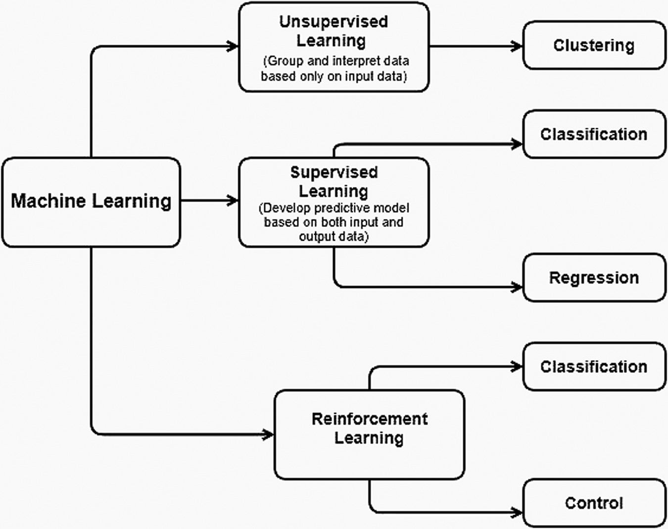
Fig. 2. Types of machine learning (adapted from Swamynathan (Reference Swamynathan2019)).
With the increasing growth of data in many sectors, the adoption of appropriate machine learning algorithms may enhance the efficiency of data analysis and processing while also solving some practical problems (Lou et al., Reference Lou, Lv, Dang, Su and Li2021). Machine learning is covered in depth in many great texts (Marsland, Reference Marsland2014; Mohri et al., Reference Mohri, Rostamizadeh and Talwalkar2018; Alpaydin, Reference Alpaydin2020). This section describes the 13 machine learning techniques performed in the study. We employed both linear (“multiple linear regression, ridge regression, lasso regression, and elastic net regression”) and nonlinear machine learning methods [“k-nearest neighbors, random forests, artificial neural network, support vector regression, classification and regression tree (CART), gradient boosting machines (GBM), extreme gradient boosting (XGBoost), light gradient boosting machine (LightGBM), and categorical boosting (CatBoost)”].
Regression modeling
In engineering, regression modeling is a highly helpful statistical approach for predicting the relationship between one or more independent variables as predictors and the dependent variables as estimated values. Multiple regression modeling is aimed in particular at understanding the change in dependent variable y and movement in k explanatory variables (independent) x 1, x 2, …, x k.
The simplest basic representation of the multiple regression analysis is as follows:
 $$\eqalign{& y_i = f( x_{i1}, \;x_{i2}, \;\ldots , \;x_{ik}) + {\in} _i, \cr & y_i = \beta _0 + \beta _1x_{i1} + \beta _2 x_{i2} + \cdots + \beta _kx_{ik} + {\in} _i.} $$
Ridge regression
Ridge regression uses the same concepts as linear regression, but adds a bias to counterbalance the impact of large variances and eliminates the necessity for unbiased estimators. It penalizes non-zero coefficients and seeks to minimize the sum of squared residuals (Hoerl and Kennard, Reference Hoerl and Kennard1970; Zhang et al., Reference Zhang, Duchi and Wainwright2015). Ridge regression performs L2 regulations that penalize the coefficients by incorporating the square of the size of the cost function coefficient:
 $$J = \mathop \sum \limits_{i = 1}^n \left({y_i-\mathop \sum \limits_{\,j = 1}^p x_{ij}\theta_j} \right)^2 + \lambda \mathop \sum \limits_{\,j = 1}^p \theta _j^2,$$
where  $\lambda \sum\nolimits_{j = 1}^p {\theta _j^2 }$ is the “regularization component”, and λ is a “regularization factor” that may be improved by evaluating the validation error.
Lasso regression
The purpose of lasso regression is to recognize the variables and associated regression coefficients leading to a model, which minimizes the prediction error. The lasso regression model, like ridge regression, penalizes the magnitude of coefficients to avoid overfitting (Vrontos et al., Reference Vrontos, Galakis and Vrontos2021). L1 regularization is performed using the lasso regression as follows:
 $$J = \mathop \sum \limits_{i = 1}^n \left({y_i-\mathop \sum \limits_{\,j = 1}^p x_{ij}\theta_j} \right)^2 + \lambda \mathop \sum \limits_{\,j = 1}^p \vert {\theta_j} \vert, $$
where  $\lambda \sum\nolimits_{j = 1}^p {\vert {\theta_j} \vert }$ is the regularization component, and it consists of the feature coefficients’ absolute values added together.
Elastic-net regression model
The elastic-net regression approach is a variation of multiple linear regression techniques for dealing with high-dimensional feature selection challenges (Fukushima et al., Reference Fukushima, Sugimoto, Hiwa and Hiroyasu2019). The penalties of the ridge and lasso techniques are linearly combined in this algorithm (Richardson et al., Reference Richardson, van Florenstein Mulder and Vehbi2021). Through the use of a parameter, 0 ≤ α ≤ 1 the elastic-net algorithm fades between the lasso and ridge techniques.
Random forests
The random forest (RF) approach (Breiman, Reference Breiman2001) is not only useful in regression and classification, but it also performs well in variable selection (Genuer et al., Reference Genuer, Poggi and Tuleau-Malot2010). RF incorporates several trees into an algorithm by including the concept of ensemble learning (Cun et al., Reference Cun, Mo, Chu, Yu, Zhang, Fan, Chen, Wang, Wang and Chen2021). Following that, the forecast for a new observation is obtained by combining the forecasted values derived from each individual tree in the forest. “The number of trees,” “the minimum number of observations in the terminal node,” and “the number of suitable features for splitting” are the three major parameters for RF algorithms. There are comprehensive mathematical explanations for RFs in the literature (Breiman, Reference Breiman2001).
k-nearest neighbors
The k-nearest neighbors (KNN) algorithm is one of mature data mining technique. KNN has therefore been recognized in data mining and machine learning as one of the top 10 algorithms (Wang and Yang, Reference Wang and Yang2020). The KNN algorithm is a supervised machine learning method that may be used to solve problems such as classification and regression (Asadi et al., Reference Asadi, Kareem, Asadi and Asadi2017). KNN collects data points that are near it. Any attributes that may change to a wide extent might effectively affect the distance between data points (James et al., Reference James, Witten, Hastie and Tibshirani2013). Then, the algorithm sorts the nearest data points from the arrival data point in terms of distance.
Artificial neural networks
ANN is a calculation technique inspired by the nervous system of the human brain that analyzes data and estimates outcomes (Rucco et al., Reference Rucco, Giannini, Lupinetti and Monti2019). ANNs are capable of working efficiently with large and complex datasets (Çakıt et al., Reference Çakıt, Karwowski, Bozkurt, Ahram, Thompson, Mikusinski and Lee2014; Noori, Reference Noori2021). The number of hidden layers in a neural network – which typically consists of an input layer, a hidden layer, and an output layer – defines the network's complexity (Haykin, Reference Haykin2007). The appropriate neural network design is a critical selection for precise prediction (Sheela and Deepa, Reference Sheela and Deepa2014). Many resources for further ANN explanations are accessible in the literature (Zurada, Reference Zurada1992; Fausett, Reference Fausett2006; Haykin, Reference Haykin2007).
Support vector regression
Support vector regression (SVR) analysis is an effective method for curve fitting and prediction for both linear and nonlinear regression types. As the conventional support vector regression formulation, Vapnik's ε-insensitive cost function is employed:
 $$\prec _\varepsilon ( e ) = Cmax( {0, \;\vert e \vert -\varepsilon } ) , \;\;\quad C > 0. $$
 In which an error  $e = y-\bar{y}$ up to $\varepsilon$ is not penalized, otherwise it will incur in a linear penalization. The “C penalization factor,” the “insensitive zone,” and the “kernel parameter” are the three hyperparameters that must be defined in the SVR model. In this research, a cross-validation procedure was performed to tune all these parameters. More discussions for further SVR explanations are accessible in the literature (Drucker et al., Reference Drucker, Burges, Kaufman, Smola and Vapnik1996).
Classification and regression tree
Classification and regression tree (CART) is a technique for partitioning variable space based on a set of rules encoded in a decision tree, where each node divides depending on a decision rule (Breiman et al., Reference Breiman, Friedman, Stone and Olshen1984). The technique may be used as a classification tree or a regression tree depending on the data type. This method aims to find the optimal split and is capable of handling huge continuous variables. The CART is built by iteratively dividing subsets of the dataset into two child nodes using all predictor variables, to produce subsets of the dataset that are as homogeneous as feasible concerning the target variable (Mahjoobi and Etemad-Shahidi, Reference Mahjoobi and Etemad-Shahidi2008).
Gradient boosting machines
Gradient boosting machines (GBMs), proposed by Friedman (Reference Friedman2001), is another approach applied for conducting supervised machine learning techniques. There are three main tuning parameters in a “gbm” model including the maximum number of trees “ntree”, the maximum number of interactions between independent values “tree depth” and “learning rate” (Kuhn and Johnson, Reference Kuhn and Johnson2013). In this work, the general parameters employed in the development of the “gbm” model were identified.
Extreme gradient boosting
The principle of the gradient boosting machine algorithm is also followed by the extreme gradient boosting (XGBoost) algorithm (Chen and Guestrin, Reference Chen and Guestrin2016). XGBoost requires many parameters, however, model performance frequently depends on the optimum combination of parameters. The XGBoost algorithm works like this: consider a dataset with m features and an n number of instances  $DS = \{ {( {x_i, \;y_i} ) \colon i = 1 \ldots n, \;\;x_i\epsilon {\rm {\mathbb R}}^m, \;y_i\epsilon {\rm {\mathbb R}}} \}$. By reducing the loss and regularization goal, we should ascertain which set of functions works best.
 $${\cal L}( \phi ) = \mathop \sum \limits_i l { ( y_i, \; \phi ( x_i) ) } + \mathop \sum \limits_k {\Omega ( {\,f_k} ) }, $$
where l represents the loss function, f k represents the (k-th tree), to solve the above equation, while Ω is a measure of the model's complexity, this prevents over-fitting of the model (Çakıt and Dağdeviren, Reference Çakıt and Dağdeviren2022).
Light gradient boosting machine
Light gradient boosting machine (LightGBM) is an open-source implementation of the gradient-boosting decision tree algorithm that uses the leaf-wise strategy to best splits that maximize gains (Ke et al., Reference Ke, Meng, Finley, Wang, Chen, Ma, Ye and Liu2017). For better prediction outcomes, several model parameters must be adjusted, including number of leaves, learning rate, maximum depth, and boosting type (Ke et al., Reference Ke, Meng, Finley, Wang, Chen, Ma, Ye and Liu2017).
Categorical boosting
Categorical boosting (CatBoost) is a gradient boosting library with the goal of reducing prediction shift during training (Prokhorenkova et al., Reference Prokhorenkova, Gusev, Vorobev, Dorogush and Gulin2018). The CatBoost technique, in contrast to other machine learning algorithms, only needs a modest amount of data training and can handle a variety of data types, including categorical features. For further information on the CatBoost algorithm, there are several resources accessible in the literature (Azizi and Hu, Reference Azizi and Hu2019).
Performance criteria
Various performance measures were used to compute the difference between actual and estimated values in the model (Çakıt and Karwowski, Reference Çakıt and Karwowski2015, Reference Çakıt and Karwowski2017; Çakıt et al., Reference Çakıt, Karwowski and Servi2020). The accuracy of the model was tested in this study to assess the effectiveness of machine learning techniques. Four performance measures were used: mean absolute error (MAE), the root mean-squared error (RMSE), the mean square error (MSE), and the coefficient of determination (R 2) to measure the performance of the methods. The model findings are more accurate when the RMSE, MSE, and MAE values are low. Higher R 2 values are a better match between the values observed and estimated. These calculations were performed using the following equations:
 $${\rm RMSE} = \sqrt {\displaystyle{1 \over n}\mathop \sum \limits_{i = 1}^n ( {P_i-A_i} ) ^2}, $$
 $${\rm MSE} = \displaystyle{1 \over n}\mathop \sum \limits_{i = 1}^n ( {P_i-A_i} ) ^2,$$
 $${\rm MAE} = \displaystyle{1 \over n}\;\mathop \sum \limits_{i = 1}^n \vert {e_i} \vert, $$
 $$R^2 = 1-\left({\displaystyle{{\mathop \sum \nolimits_{i = 1}^n {( P_i-A_i) }^2} \over {\mathop \sum \nolimits_{i = 1}^n A_i^2 }}} \right),$$
where “Ai” and “Pi” are the measured (experimental) and estimated parameters, respectively,
ei is “the prediction error”; n is “total number of testing data”
 $$i = 1, \;2, \;3, \;\ldots, \;n.$$
Results and discussion
Model evaluation
Python/Jupyter Notebook was used for model developing, and all machine learning methods were implemented using the scikit-learn packages (Scikit-Learn: Machine Learning in Python, 2021). RMSE, MSE, MAE, and R 2 statistics were provided and the model results followed real values slightly for the performed multiple regression model (Fig. 3a). Similarly, Figure 3b shows a comparison between the forecasted and the ridge regression output. The ridge regression results show that the real values are somewhat followed by the predicted values. For the developed lasso regression model, RMSE, MSE, MAE, and R 2 statistics were provided and the model results followed real values slightly (Fig. 3c). On the basis of the elastic-net regression model results, 59.02, 3483.29, 24.50, and 0.557 were reported for the RMSE, MSE, MAE and R2 values, respectively (Fig. 3d).

Fig. 3. Actual and predicted values for linear models (regression models).
Similarly, RMSE, MSE, MAE, and R 2 statistics were provided for nonlinear models. On the basis of the random forests model results, 8.89, 79.18, 2.76, and 0.989 were reported for the RMSE, MSE, MAE, and R 2 values, respectively (Fig. 4a). Based on the KNN model results, 1.48, 2.20, 0.91, and 0.998 were reported for the RMSE, MSE, MAE, and R 2 values, respectively (Fig. 4b). The outputs of the KNN model show that the actual values are closely followed. MLP from the scikit-learn library was conducted in this study. It was decided to use the following criteria: (“alpha = 0.01, beta_1 = 0.8, beta_2 = 0.999, epsilon = 1 × 10−07, hidden layer sizes = (100,100), learning_rate_init = 0.002, max_iter = 300, momentum = 0.9, n_iter_no_change = 10”). According to the ANN model results, 61.17, 3742.60, 32.95, and 0.998 were reported for the RMSE, MSE, MAE, and R 2 values, respectively (Fig. 4c). The support vector machines class of the sklearn python library was used to select the model parameters for this study (C = 0.2,  $\varepsilon$ = 0.05, and kernel = “rbf”) and the support vector regression model was imported.

Fig. 4. Actual and predicted values for nonlinear models.
On the basis of the support vector regression model results, 9.41, 8.62, 3.89, and 0.920 were reported for the RMSE, MSE, MAE, and R 2 values, respectively (Fig. 4d). For the developed CART model, RMSE, MSE, MAE, and R 2 statistics were provided and the model results were shown to closely follow real values (Fig. 4e). For GBM model development, the following parameters were selected: (“learning rate”: 0.02, “loss”: “ls”, “max depth”: 2, “n estimators”: 500, “subsample”: 1). The remaining parameters were left with the default settings. The “gbm” development was then initiated using the provided parameters. RMSE, MSE, MAE, and R 2 statistics were provided and the model results were shown to closely follow real values for the performed GBM model (Fig. 4f).
10-fold cross-validation was used to tune the parameters and launched “xgb” development using the parameters provided to it. Based on the optimum parameters (“colsample bytree”: 1, “learning rate”: 0.02, “max depth”: 3, “n estimators”: 500), the developed “xgb” model was selected. On the basis of the “xgb” model results, 41.31, 1707.07, 17.51, and 0.782 were reported for the RMSE, MSE, MAE, and R 2 values, respectively (Fig. 4g). For “lightgbm” model development, trial-and-error methods were used to set the parameters, and the developed “lightgbm” model based was selected (“learning rate”: 0.2, “max depth”: 2, “n_estimators”: 30). On the basis of the “lightgbm” model results, 51.37, 2639.71, 25.40, and 0.664 were reported for the RMSE, MSE, MAE, and R 2 values, respectively (Fig. 4h). The “CatBoost” algorithm was conducted with the required parameters (“learning rate,” “the maximum depth of the tree,” etc.) in this research. The best parameters (“depth”: 2, “iterations”: 500, “learning rate”: 0.09) were used to choose the developed “CatBoost” model. On the basis of the “CatBoost” model results, 44.31, 1963.91, 19.64, and 0.750 were reported for the RMSE, MSE, MAE, and R 2 values, respectively (Fig. 4i).
Comparison of the algorithm performance
Performance criteria were used to assess the algorithms on the same basis in order to investigate the effectiveness of modeling strategies in forecasting the standard time and to choose the best strategy among the machine learning approaches employed in this study. Based on the comparison of performance metrics, the KNN algorithm outperformed other machine learning approaches in estimating the standard time (Table 1). Figure 5 shows that the KNN outputs closely follow the actual values. The results of the paired t-test analysis show that there was statistically no significant difference between actual and estimated standard time testing data based on the KNN method at the α value of 0.05 (p = 0.193). Gradient boosting machines are in second place in terms of performance compared to the KNN method and RMSE findings. The RF method surpasses the classification and regression tree approach, which is ranked fourth. The extreme gradient boosting algorithm was unable to exceed KNN performance. Based on the findings acquired using machine learning methods, the standard time can be easily and accurately predicted based on various parameters including the number of products, the number of welding operations, product's surface area factor, difficulty/working environment factor, and the number of metal forming processes.

Fig. 5. Predicted and actual values of KNN algorithm.
Table 1. Comparison of algorithm performance

Sensitivity analysis
In the previous section, the KNN algorithm outperformed other machine learning approaches in terms of prediction accuracy. To what degree the input parameters contribute to the determination of the output parameter was determined via a sensitivity analysis using the KNN technique. Based on the results obtained in Figure 6, the most effective parameter was determined to be “the number of welding operations”. Another input variable was found to be another efficient parameter, namely, “the number of pieces.”

Fig. 6. Sensitivity analysis results.
Comparison with previous studies
Differently from the previous study by Dağdeviren et al. (Reference Dağdeviren, Eraslan and Çelebi2011), more data were collected to build and test 13 machine learning algorithms to predict the standard time. In comparison to Dağdeviren et al. (Reference Dağdeviren, Eraslan and Çelebi2011), and to learn more about the prediction capability of the KNN method, forecasting accuracy was compared on the basis of RMSE values. Based on the results in Table 2, the calculated RMSE of KNN algorithm was 1.48, indicating that the predictive accuracy for the KNN algorithm developed in this study has a higher prediction accuracy than the models developed by Dağdeviren et al. (Reference Dağdeviren, Eraslan and Çelebi2011).
Table 2. Performance comparison with previous studies

Conclusion
Some of the biggest problems with today's sophisticated manufacturing systems can be solved using machine learning approaches. These data-driven approaches are capable of identifying extremely intricate and nonlinear patterns in data from various types and sources. They convert raw data into feature spaces, or models, which are then used not only for prediction, as in the case of this study, but also for detection and classification in manufacturing settings. Machine learning has also been effectively applied in various manufacturing settings for process optimization, monitoring, and control (Gardner and Bicker, Reference Gardner and Bicker2000; Pham and Afify, Reference Pham and Afify2005; Kwak and Kim, Reference Kwak and Kim2012; Susto et al., Reference Susto, Schirru, Pampuri, McLoone and Beghi2015).
This study was aimed primarily at using machine learning algorithms to predict the standard time based on various parameters, including the number of products, the number of welding operations, product's surface area factor, the difficulty of the working environment, and the number of metal forming processes. To obtain the best results in terms of RMSE, MSE, MAE, and R 2 values, 13 machine learning algorithms were used, including linear and nonlinear models. When the performance values were calculated, the estimated output values provided using the KNN method were determined to be the most satisfactory. The number of welding operations and the number of pieces were the two most sensitive variables, accounting for nearly 90% of the sensitive weights. Machine learning algorithms are largely reliable based on their capacity to learn from past data. To improve the effectiveness of machine learning techniques, additional research using machine learning methods should gather more training records and incorporate other factors when conducting future studies.
Employing the suggested estimate technique and designating people specifically for this task might be very beneficial for businesses who do not know the true standard time of their items due to measurement issues. Therefore, the study's prediction results can be applied in various ways, such as by reducing manufacturing costs, increasing productivity, minimizing time study experiments, and ensuring efficiency in the execution of manufacturing processes. In addition to reducing the total cost, the obtained results may shorten time measurements and enhances standard time accuracy.
The main limitation of the study is the fact that the machine learning algorithms may not be easily applicable to every product or semi-product, many of which have complicated production processes, and it is difficult to establish the time-affecting factors in each situation.
Conflict of interest
The authors declare no competing interests.
Erman Çakıt received his Ph.D. in Industrial Engineering from the University of Central Florida,Orlando, USA, in 2013. He is currently working as a Professor at the Department of Industrial Engineering, Gazi University, Turkey. His research interests include applications of human factors / ergonomics and safety using machine learning and applied statistics. He has authored more than 50 papers published as peer reviewed journal articles, book chapters and conference proceedings.He serves as a Associate Editor of Ergonomics International Journal, and editorial board member in Human-Intelligent Systems Integration (Springer),Augmented Human Research (Springer), International Journal of Machine Learningand Computing, Advances in Artificial Intelligence and Machine Learning.
Metin Dağdeviren is a Professor in the Department of Industrial Engineering at Gazi University, Ankara, Turkey and Higher Education Auditing Council Member at Council of Higher Education, Ankara, Turkey. He received his Ph.D. in Industrial Engineering from the Gazi University, Ankara, Turkey. He is the author or coauthor of over 200 scientific publications which focus on human factors engineering, multi criteria decision making, process management and decision making in fuzzy environment.


 Open access