


1. Introduction
Crude mortality rates often exhibits natural randomness and irregular patterns. Graduation or modelling of mortality rates refers to the act of smoothing crude mortality rates. Sometimes extrapolation to higher ages is also performed during the process since the usual assumed maximum lifespan of humans (e.g. 125) is often beyond the range of available data. Mortality rates are usually expressed in the form of life tables, which contains the number of expected lives and deaths at different ages. Life tables are widely used in the insurance sector as there are many insurance products related to mortality.
Several methods have been proposed in the past, however, due to the peculiar shape of the human mortality curve (e.g. accident hump in late teens, very high infant mortality rates), these methods often involve relatively complicated mathematical functions. It is only recently that non-parametric smoothing techniques have become popular and are employed in graduation of mortality rates. These non-parametric methods are more flexible and they do not assume any particular decomposition of the mortality schedule.
Mortality graduation models, sometimes also called “laws of mortality”, have become more sophisticated over time. One of the earliest models, Gompertz law of mortality (1825), states that the mortality rates is an exponential function of age, i.e. the log of mortality rates is linear in age. The law is then extended by Makeham in 1860 to the Gompertz–Makeham law where he proposed the addition of a constant, which captures mortality due to age-independent accidents. In spite of the simple and interpretable functions, these laws provide adequate fit to only limited age range, say 30–90, where the log-linearity assumption seems appropriate. The constant rate of increase (i.e. the log-linearity) in mortality rates might not be suitable at the very old ages. In fact, a decelerating rate of increase is often observed at these ages (Carriere, Reference Carriere1992). Perks (Reference Perks1932), Beard (Reference Beard1959) and Thatcher (Reference Thatcher1999) suggested to use logistic functions so that the mortality rates tend to an asymptote. At younger ages where mortality rates are lower, the logistic curve behaves similarly to the Gompertz or Gompertz–Makeham laws. Lindbergson (Reference Lindbergson2001) suggested a piecewise model such that for ages less than a cut-off age the mortality rates follow the Gompertz–Makeham law, while after the cut-off age they are modelled by a linear function. Saikia & Borah (Reference Saikia and Borah2014) did a comparative study on models for the oldest ages and showed that the logistic model is the most reasonable choice amongst the laws mentioned above. More recently, Pitacco (Reference Pitacco2016) provides a comprehensive review of old age models.
The models discussed so far are only applicable to the adult ages. Several more complicated mathematical functions have been proposed in an attempt to model mortality rates for the entire age range. Heligman & Pollard (Reference Heligman and Pollard1980) proposed the eight parameters Heligman–Pollard Model. Carriere (Reference Carriere1992) modelled the survival function and viewed it as a mixture of infant, young adult and adult survival functions. Despite the ability to model mortality rates of the whole age range with interpretable parameters, these models are often difficult to fit in practice, due to the high correlation in the estimated parameters. The high correlation also compromises interpretability.
Recently more flexible, non-parametric smoothing approaches are used to model mortality. These methods are used to produce the English Life Tables (ELTs), decennial life tables published by the Office for National Statistics (ONS) in every 10 years after every census. Since the 13th English Life Table (ELT13), subsequent ELTs are all produced using spline-based methods. In ELT14, a variable knot cubic spline is adopted and the optimal number and location of knots are estimated. In ELT15, a weighted least squares smoothing spline is used, with a modification that the user specifies a set of weights based on their judgment in respect of the regions where the closest fit should be expected. In addition, some data at the highest ages are discarded to maintain a monotonic (upward) progression in the graduated mortality rates. In ELT16, a Geometrically Designed variable knot regression spline (Kaishev et al., Reference Kaishev, Dimitrova, Haberman and Verrall2006) is used. This is a two-stage method where they first fit a variable knots linear spline, and then estimate the optimal control polygon of higher order splines, resulting in estimates of the optimal knot sequence, the order of the spline and the spline coefficients all together. Detailed information on methods used in the production of ELTs can be found in Gallop (Reference Gallop2002). In the latest English Life Table, ELT17, Dodd et al. (Reference Dodd, Forster, Bijak and Smith2018) suggest to use a hybrid function for graduation. Specifically, mortality rates before some cut-off age are modelled using splines while mortality rates after the cut-off age are modelled using a parametric model (log-linear or logistic). At younger ages, there is sufficiently dense data, therefore, the flexibility of splines makes it a very effective tool in graduating mortality rates at these ages, whereas at the oldest ages, a parametric function helps produce more robust estimates and extrapolation. The final graduation combines different threshold ages with weights determined by cross-validation error. This requires multiple fits and the transition from spline to the parametric model is not guaranteed to be smooth.
We extend the approach presented in Dodd et al. (Reference Dodd, Forster, Bijak and Smith2018) by using adaptive splines. Under this approach, instead of splitting the age into non-parametric and parametric regions, a P-spline is used for the whole age range with adaptive penalty. Contrary to traditional P-splines, instead of having a single smoothing parameter governing the overall smoothness, adaptive splines allow varying smoothness over the domain, hence enhancing flexibility and giving better fit to functions with changing smoothness. Ruppert & Carroll (Reference Ruppert and Carroll2000) showed that even when the true underlying function is uniformly smooth, adaptive splines perform at least as well as traditional splines in terms of model fit. Different approaches have been suggested to estimate the varying smoothness penalty. Pintore et al. (Reference Pintore, Speckman and Holmes2006) and Liu & Guo (Reference Liu and Guo2010) used piecewise constant functions for the varying penalty. Ruppert & Carroll (Reference Ruppert and Carroll2000) and Krivobokova et al. (Reference Krivobokova, Crainiceanu and Kauermann2008) proposed to use a second layer of spline for the penalty. Storlie et al. (Reference Storlie, Bondell and Reich2010) suggested to estimate the changing smoothness from an initial fit with an ordinary spline while Yang & Hong (Reference Yang and Hong2017) recommended to weight the penalty inversely to the volatility of the data in proximity. Bayesian adaptive splines have also been investigated (see Baladandayuthapani et al. (Reference Baladandayuthapani, Mallick and Carroll2005), Crainiceanu et al. (Reference Crainiceanu, Ruppert, Carroll, Joshi and Goodner2007), Jullion & Lambert (Reference Jullion and Lambert2007) and Scheipl & Kneib (Reference Scheipl and Kneib2009)). In addition to smoothness, shape-constrained splines have also been proposed so that the resulting estimated splines satisfy some presumed functional form. Pya & Wood (Reference Pya and Wood2015) demonstrated how to achieve different shape constraints by re-parameterisation of the spline coefficients while Bollaerts et al. (Reference Bollaerts, Eilers and Van Mechelen2006) controlled the shape through iteratively adding asymmetric penalties. Camarda et al. (Reference Camarda, Eilers and Gampe2016) proposed a sums of smooth exponentials model and demonstrated it for mortality graduation using shape-constrained P-splines. Camarda (Reference Camarda2019) applied shape constraints in the context of mortality forecasting.
The English Life Tables present smooth mortality rates for males and females. Although male and female mortality rates show similar patterns, male mortality rates are expected to be higher than female mortality rates at any age. When males and female mortality rates are modelled separately, problems may arise such as crossing-over rates at very high ages, where data are sparse, or a decreasing mortality trend in age. In the previous ELTs, these problems are addressed using rather ad hoc approaches. For example, in ELT14, an arbitrary value is chosen as the mortality rate at the closing age, while in ELT15, the data at the highest ages are discarded as it would produce downwards mortality profile otherwise. In ELT17, the male and female mortality rates are calculated as the weighted average of the respective graduated mortality rates starting at the age where they cross-over.
Various multi-population models have been proposed in the context of coherent mortality forecasting. Many of these concern the correlation between the period effects of different populations, for example, the common factor model by Li & Lee (Reference Li and Lee2005) assumed that different populations share the same age-period effect, who further proposed the augmented common factor model where additional population specific age-period terms are included for a better fit, which are mean reverting in the long run. Cairns et al. (Reference Cairns, Blake, Dowd, Coughlan and Khalaf-Allah2011) modelled mortality for two populations and assumed that the spread between the period effects (and cohort effects) of the two populations are mean reverting. Dowd et al. (Reference Dowd, Cairns, Blake, Coughlan and Khalaf-Allah2011) also proposed a similar model where in addition to having mean-reverting spread between the time series, the period effect (and cohort effect) of a smaller population is actually being “pulled” towards that of the larger population, hence in the long run the projected mortality rates converge.
Another class of models is the relational models where usually a reference mortality schedule is first modelled and then the spread/ratio between another population of interest and the reference schedule. For example, Hyndman et al. (Reference Hyndman, Booth and Yasmeen2013) proposed the Product-Ratio Model where the geometric mean of the populations are modelled as the reference schedule and the ratios are assumed to follow stationary processes so as to produce non-divergent forecasts. Villegas & Haberman (Reference Villegas and Haberman2014) modelled the mortality of different socio-economic subpopulations. Jarner & Kryger (Reference Jarner and Kryger2011) proposed the SAINT model, where they model the ratio between the mortality rates of a subpopulation to the reference using some orthogonal regressors. Biatat & Currie (Reference Biatat and Currie2010) extended the 2D spline model by Currie et al. (Reference Currie, Durban and Eilers2004) to a joint model by adding another 2D spline for the spread of a population to a reference population.
Limited focus has been placed on the convergence of the age patterns of male and female mortality. Plat (Reference Plat2009) modelled the ratio between a subpopulation and a main population and assumed the ratio to be one after a certain age, this is because the difference between the subpopulation mortality and main population mortality is expected to diminish at higher ages. Hilton et al. (Reference Hilton, Dodd, Forster and Smith2019), on the other hand, used a logit link and assumed a common asymptote for males and females. In this paper, we propose a coherent method for jointly smoothing male and female mortality rates. Our method allows us to borrow information, especially in areas where data are scarce and unreliable. The convergence of the male and female mortality curves is achieved by means of penalty.
In this paper, we propose a model for mortality graduation using adaptive splines. This model is able to produce smooth mortality schedules for the entire age range and it is robust at the oldest ages where data are sparse. We also model male and female mortality rates together as modelling them independently causes inconsistencies such as divergent or intersecting trends, especially at the oldest ages. This is often addressed using ad hoc methods (e.g. see previous ELTs). The joint model proposed in this paper does not require such interventions and is able to produce non-divergent and non-intersecting male and female mortality schedules. It also allows strength to be borrowed across sexes at the oldest ages which further increases robustness. More details can be found in Tang (Reference Tang2021).
The rest of the paper is structured as follows: in section 2, the data are described and some notes on general mortality pattern are discussed. In section 3, we introduce our methodology and present our results. In section 4, the model is extended to model male and female mortality rates jointly. Finally, we provide a brief conclusion in section 5.
2. Data
The data we use in this paper contains the number of deaths and mid-year population estimates by single year of age for males and females in England and Wales from 2010 to 2012 obtained from the Office for National Statistics (2019). Data by single age is available up to the age of 104 for both males and females, while data at the age of 105 and above are aggregated into one age group. Typically infant mortality rates are dealt with separately, therefore infant data are excluded, leaving us with data spanning from ages 1 to 104. The central mortality rate at age x,
 $m_x$
is defined as
$m_x$
is defined as
 \begin{align}m_x = \frac{d_x}{E^C_x}\end{align}
where
 $d_x$
and
$d_x$
and
 $E^C_x$
are the number of deaths and central exposure at age
$E^C_x$
are the number of deaths and central exposure at age
 $[x, x+1)$
, respectively. The crude central mortality rates
$[x, x+1)$
, respectively. The crude central mortality rates
 $\tilde{m}_x$
are then obtained by approximating the central exposure with the mid-year population estimates. Furthermore, it is assumed that the number of deaths at each age follow a Poisson distribution,
$\tilde{m}_x$
are then obtained by approximating the central exposure with the mid-year population estimates. Furthermore, it is assumed that the number of deaths at each age follow a Poisson distribution,
 \begin{align}d_x \sim \text{Poisson} (E^C_x m_x)\end{align}
Figure 1 shows the crude mortality rates for each year on a logarithmic scale. As expected, mortality is decreasing at child ages until around mid-teenage, followed by a sudden increase in mortality rates at late teenage, so-called “accident hump”. Afterwards, the mortality increases steadily due to senescence. Male mortality rates lie above female mortality rates at almost all ages and that they are converging at the end. A decreasing rate of increase in mortality also seems to be taking place at the oldest ages. The crude mortality rates at the youngest and the oldest ages are more dispersed than those in the middle due to the sparsity of data at these ages.

Figure 1 Crude mortality rates England and Wales. Blue and red points are the male and female crude mortality rates, respectively.
3. Methodology
In this section, we introduce our proposed model. Before moving onto the model specifics, first, we shall have a look at the robustness problem when ordinary P-spline smoothing is used. Splines are piecewise polynomials that are continuous up to certain order of derivatives and P-splines are one of the most commonly used splines having a B-spline basis with discrete penalties (Eilers & Marx, Reference Eilers and Marx1996). We use ordinary P-splines with 40 basis functions with equally spaced knots, and males and females have the same basis. The basis dimension is chosen according to preliminary analysis. The data are fitted with ordinary P-splines of dimension 20, 25, 30, 35, 40, 45, 50, 55, 60, 65 for each sex and the total effective degrees of freedom for males and females is examined. The total effective degrees of freedom starts to level off at around 40 basis functions for each sex (80 total dimension), indicating that further increase in the dimension has limited benefits. Note that there is no unified approach for choosing the dimension since the essence of penalised splines is that the user constructs a basis that is generous enough to capture the fluctuations of the underlying function and then penalises the roughness to prevent overfitting.
Fitting the ordinary P-spline to the mortality data, several problems are revealed. Figure 2 plots the ordinary P-spline fits to the data. The circles and crosses are the crude mortality rates. The solid lines are the fits using data from ages 1 to 104, while the dotted lines are the fits using data only up to the age of 100 (excluding the crosses). From Figure 2, it is clear that the fit to the oldest ages is not robust, and the yearly variation in mortality pattern is irregular. Comparing the solid and dotted lines, the exclusion of the last four data points (crosses) changes the shapes quite drastically, again revealing the lack of robustness. Extrapolation based on these trends is very sensitive to the unreliable data at the oldest ages. Sometimes an unreasonable mortality schedule can also be obtained, for instance, the estimated mortality rates for males in 2010 is decreasing at the oldest ages.
The root cause for the lack of robustness at high ages is that ordinary P-splines have only one smoothing parameter governing the overall smoothness, hence resulting in either over-smoothed young mortality rates (less likely due to the much bigger exposures than older ages) or under-smoothed old mortality rates.This motivates the use of P-splines with varying smoothness penalty. Contrary to a global smoothing parameter in ordinary P-spline tuning the overall smoothness, the smoothness penalty over the domain is allowed to vary. This is sometimes called “adaptive smoothing” or “adaptive spline”. Ruppert & Carroll (Reference Ruppert and Carroll2000) have shown that adaptive smoothing is more effective and gives better results than ordinary splines especially when the underlying function has varying smoothness. Here, we suggest using an exponential function for the smoothness penalty. This is because the mortality pattern is expected to be increasingly smooth in age and having a heavier smoothness penalty at the oldest ages means that more strength is borrowed from neighbouring ages, therefore improving the robustness. Alternatively, linear or piecewise constant functions could be used for the smoothness penalty. However, the linear function would not be as effective as the exponential function here as we require very low penalty at younger ages where there is plenty of data and significantly higher penalty at the oldest ages where data are sparse. On the other hand, a piecewise constant function would require estimation of the levels and locations of the jumps. In our case, we do not believe that this additional computational burden is justified. Using exponential function for the smoothness penalty we have
 \begin{align}\begin{split}d_x \sim \text{Poisson} &(E^C_x m_x), \, \text{where} \, \log (m_x) = {\textbf{\textit{b}}_x^{\prime}} \, \boldsymbol{\beta} \\ \qquad \text{with penalty} \, \sum^{k}_{i=3} &\zeta(i) (\bigtriangledown^2(\beta_i))^2 \text{ and } \zeta(i)\, = \, \lambda_1 \, \exp(\, \lambda_2 \, i ), \, \lambda_1 > 0\end{split}\end{align}
Here,
 $\bigtriangledown^2$
is the second difference operator,
$\bigtriangledown^2$
is the second difference operator,
 $\textbf{\textit{b}}_x^{\prime}$
is the row corresponding to age x of the design matrix
$\textbf{\textit{b}}_x^{\prime}$
is the row corresponding to age x of the design matrix
 $\textbf{\textit{B}}$
of the B-spline basis with the corresponding coefficient vector
$\textbf{\textit{B}}$
of the B-spline basis with the corresponding coefficient vector
 $\boldsymbol{\beta}$
,
$\boldsymbol{\beta}$
,
 $\lambda_1$
and
$\lambda_1$
and
 $\lambda_2$
are smoothing parameters and k is the dimension of the basis. The penalty can be written more compactly as
$\lambda_2$
are smoothing parameters and k is the dimension of the basis. The penalty can be written more compactly as
 $\boldsymbol{\beta}'\textbf{\textit{P}}'\boldsymbol{\Lambda}\textbf{\textit{P}}\boldsymbol{\beta}$
where
$\boldsymbol{\beta}'\textbf{\textit{P}}'\boldsymbol{\Lambda}\textbf{\textit{P}}\boldsymbol{\beta}$
where
 $\textbf{\textit{P}}$
is the second-order difference matrix with appropriate dimensions and
$\textbf{\textit{P}}$
is the second-order difference matrix with appropriate dimensions and
 $\boldsymbol{\Lambda}$
is a diagonal matrix with
$\boldsymbol{\Lambda}$
is a diagonal matrix with
 $\boldsymbol{\Lambda}_{ii} =\lambda_1 e^{\lambda_2 \, i}$
.
$\boldsymbol{\Lambda}_{ii} =\lambda_1 e^{\lambda_2 \, i}$
.

Figure 2 (a) England and Wales males (b) England and Wales females Ordinary P-spline fits extrapolated to the age of 120. The solid lines are the estimated mortality rates using data from ages 1 to 104, while the dotted lines are the estimated mortality rates using data only from ages 1 to 100.
When the smoothing parameters
 $\lambda_1$
and
$\lambda_1$
and
 $\lambda_2$
are known or specified, the fitting of the spline coefficients is straightforward by maximising the penalised likelihood. Otherwise, they can be estimated together with the spline coefficients from the data. Here, we estimate
$\lambda_2$
are known or specified, the fitting of the spline coefficients is straightforward by maximising the penalised likelihood. Otherwise, they can be estimated together with the spline coefficients from the data. Here, we estimate
 $\lambda_1$
and
$\lambda_1$
and
 $\lambda_2$
by minimising the Bayesian Information Criterion (BIC). The Newton–Raphson method can be used to estimate the optimal smoothing parameters within each working model of the Penalised Iteratively Re-weighted Least Squares (P-IRLS) iteration, namely the performance iteration (Gu, Reference Gu1992; Wood, Reference Wood2006). The relevant gradient and Hessian for the minimisation of BIC can be found in the Appendix A. The BIC surface is relatively flat at regions with very low or very high penalty, hence these regions should be avoided as initial estimates. Alternatively, a two-dimensional grid search could be employed, the gradients and Hessian are prepared for the sake of the joint model in section 4, which contains six smoothing parameters and hence reduces the efficiency of grid search.
$\lambda_2$
by minimising the Bayesian Information Criterion (BIC). The Newton–Raphson method can be used to estimate the optimal smoothing parameters within each working model of the Penalised Iteratively Re-weighted Least Squares (P-IRLS) iteration, namely the performance iteration (Gu, Reference Gu1992; Wood, Reference Wood2006). The relevant gradient and Hessian for the minimisation of BIC can be found in the Appendix A. The BIC surface is relatively flat at regions with very low or very high penalty, hence these regions should be avoided as initial estimates. Alternatively, a two-dimensional grid search could be employed, the gradients and Hessian are prepared for the sake of the joint model in section 4, which contains six smoothing parameters and hence reduces the efficiency of grid search.
In Figure 3, we present the fitted mortality rates for our model. Compared to the ordinary P-spline fit in Figure 2, we can see that the fit is more robust at high ages under the exponentially increasing penalty. The yearly mortality pattern is more reasonable with less irregular variations. The spline is also capable of capturing the decreasing rate of increase in the oldest mortality rates. Figure 4 shows the P-spline fit for males in 2011 and the corresponding estimate of the exponential penalty. The increase in smoothness takes effect at around the age of 90, which is desirable as this is the region where the exposures and hence the reliability start to drop.

Figure 3 (a) England and Wales males (b)England and Wales females Adaptive exponentially increasing penalty P-spline fit to the period mortality schedule extrapolated to the age of 120.

Figure 4 P-spline with exponential penalty fit for 2011 England and Wales males and the corresponding adaptive smoothness penalty.
4. Joint Model
We have been modelling male and female data separately. However, jointly modelling male and female mortality rates has several advantages, such as avoiding cross-over at the highest ages and allowing borrowing of strength. Male and female mortality rates often display converging trends at high ages, information could be shared between the two sexes. This will produce coherent estimates especially at ages with low exposures as we are pooling the two data sets. On top of the exponential smoothness penalty for males and females, an additional penalty on the difference between the male and female P-spline coefficients is introduced. As stated before, males and females have the same P-spline basis.
At earlier ages, the splines shall enjoy more freedom as data at this region is more reliable. It is also believed that there is genuine difference in the levels and patterns of mortality between male and female mortality (especially for the accident hump). At adult ages, the difference between male and female mortality rates seems to diminish gradually as age increases. Therefore, an exponential penalty will be used again such that at younger ages the male and female coefficients are expected to be penalised less. In our applications, it is found that estimation is easier when the differences between the first few male and female coefficients are left un-penalised. We suspect this is due to the apparent converging trend at the youngest ages as well. Therefore, we only apply the difference penalty after a certain basis function. In our experiments, the selection of this coefficient is immaterial as long as it excludes childhood mortality. Here, the difference penalty is chosen to start at the ninth coefficient (around the age of 24, which is just after the accident hump). The model is
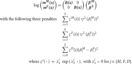 \begin{align}\log \begin{pmatrix} \textbf{\textit{m}}^{\textbf{\textit{M}}}\textbf{\textit{(x)}} \nonumber\\ \textbf{\textit{m}}^{\textbf{\textit{F}}}\textbf{\textit{(x)}} \end{pmatrix} = &\begin{pmatrix} \textbf{\textit{B(x)}} & 0 \\ 0 & \textbf{\textit{B(x)}} \end{pmatrix} \begin{pmatrix} \boldsymbol{\beta}^{\textbf{\textit{{M}}}} \nonumber\\ \boldsymbol{\beta}^{\textbf{\textit{F}}} \end{pmatrix} \nonumber\\ \text{with the following three penalties} \quad &\sum^{k}_{i=3} \zeta^M(i) (\bigtriangledown^2(\beta^M_i))^2 \nonumber\\&\sum^{k}_{i=3} \zeta^F(i) (\bigtriangledown^2(\beta^F_i))^2 \nonumber\\&\sum^{k}_{i=9} \zeta^D(i) (\beta^M_i-\beta^F_i)^2 \nonumber\\\text{where } \zeta^{j}(\boldsymbol{\cdot})\, = \, \lambda^{j}_1 \, &\exp(\, \lambda^{j}_2 \, \boldsymbol{\cdot}), \text{ with } \lambda^j_1 > 0 \text{ for } j \in \{ M, F, D \}.\end{align}
The first two penalties relate to the smoothness of male and female mortality rates while the third penalty corresponds to the difference between male and female mortality rates. The penalties can be written more compactly as
 $\boldsymbol{\beta}'\textbf{\textit{P}}'\textbf{\textit{P}}\boldsymbol{\beta}$
where the overall coefficient vector is
$\boldsymbol{\beta}'\textbf{\textit{P}}'\textbf{\textit{P}}\boldsymbol{\beta}$
where the overall coefficient vector is
 $\boldsymbol{\beta} = (\begin{smallmatrix} \boldsymbol{\beta}^{\textbf{\textit{M}}} & \boldsymbol{\beta}^{\textbf{\textit{F}}} \end{smallmatrix})$
and the overall penalty matrix is
$\boldsymbol{\beta} = (\begin{smallmatrix} \boldsymbol{\beta}^{\textbf{\textit{M}}} & \boldsymbol{\beta}^{\textbf{\textit{F}}} \end{smallmatrix})$
and the overall penalty matrix is
 $\textbf{\textit{P}} = \bigg(\begin{smallmatrix} \sqrt{\boldsymbol\Lambda^{\textbf{\textit{M}}} \textbf{\textit{P}}^{\textbf{\textit{M}}}} \\ \boldsymbol{\sqrt{\Lambda^F} P^F} \\ \boldsymbol{\sqrt{\Lambda^D} P^D}\end{smallmatrix}\bigg)$
,
$\textbf{\textit{P}} = \bigg(\begin{smallmatrix} \sqrt{\boldsymbol\Lambda^{\textbf{\textit{M}}} \textbf{\textit{P}}^{\textbf{\textit{M}}}} \\ \boldsymbol{\sqrt{\Lambda^F} P^F} \\ \boldsymbol{\sqrt{\Lambda^D} P^D}\end{smallmatrix}\bigg)$
,
 $\textbf{\textit{P}}^{\textbf{\textit{M}}} = (\begin{smallmatrix} \boldsymbol{\nabla_2} & {\bf 0} \end{smallmatrix})$
,
$\textbf{\textit{P}}^{\textbf{\textit{M}}} = (\begin{smallmatrix} \boldsymbol{\nabla_2} & {\bf 0} \end{smallmatrix})$
,
 ${\textbf{\textit{P}}^{\textbf{\textit{F}}} = (\begin{smallmatrix} \textbf{\textit{0}} & {\boldsymbol\nabla_{\bf 2}} \end{smallmatrix})}$
. Here
${\textbf{\textit{P}}^{\textbf{\textit{F}}} = (\begin{smallmatrix} \textbf{\textit{0}} & {\boldsymbol\nabla_{\bf 2}} \end{smallmatrix})}$
. Here
 $\boldsymbol{\nabla}_{\textbf{\textit{2}}}$
is the second-order difference matrix,
$\boldsymbol{\nabla}_{\textbf{\textit{2}}}$
is the second-order difference matrix,
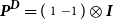 $\textbf{\textit{P}}^{\textbf{\textit{D}}} = (\begin{smallmatrix} 1 & -1\end{smallmatrix} ) \otimes \textbf{\textit{I}} $
and
$\textbf{\textit{P}}^{\textbf{\textit{D}}} = (\begin{smallmatrix} 1 & -1\end{smallmatrix} ) \otimes \textbf{\textit{I}} $
and
 $\textbf{0}$
is simply a null matrix of appropriate dimension.
$\textbf{0}$
is simply a null matrix of appropriate dimension.
Figure 5 shows the results of the modelling. When males and females are modelled separately (dotted lines), the extrapolated trends sometimes diverge, which is not desirable. A clearer example would be the year 2007 where the dotted lines drift apart (Figure 6). The difference penalty prevents divergence and further increases the robustness when extrapolating to higher ages even without data by learning from the existing data how fast and strongly the two trends should converge.

Figure 5 (a) Full age range (b) Ages 70–120 P-spline fit with cross-sex penalty extrapolated to the age of 120. The dotted lines correspond to the fits without the cross-sex penalty (i.e. fitted separately) and the solid lines correspond to the fits with cross-sex penalty.

Figure 6 P-spline fit with cross-sex penalty extrapolated to the age of 120 for the year 2007. The dotted lines correspond to the fits without the cross-sex penalty (i.e. fitted separately) and the solid lines correspond to the fits with cross-sex penalty.
4.1 Preventing cross-over
One final improvement for the model is that, while the difference penalty dictates the convergence of male an female mortality curves, there is no guarantee that the graduated male mortality rates will always be higher than the female mortality rates. For instance, in Figure 5(a), the male and female mortality estimates for 2012 cross-over at around the age of 10. Sometimes this could also happen at the oldest ages or extrapolated range. To deny the possibility of male and female mortality rates crossing over, we impose a hard constraint on the coefficients such that the each of the B-spline coefficients for males are greater than or equal to that for females, i.e.
 $\boldsymbol{\beta}^{\textbf{\textit{M}}} \boldsymbol\geq \boldsymbol\beta^{\textbf{\textit{F}}}$
. Since it is assumed that males and females have the same knot sequence, this is a sufficient condition such that
$\boldsymbol{\beta}^{\textbf{\textit{M}}} \boldsymbol\geq \boldsymbol\beta^{\textbf{\textit{F}}}$
. Since it is assumed that males and females have the same knot sequence, this is a sufficient condition such that
 $\, m^F(x) \, \leq \, m^M(x) \quad \forall x$
. In other words, the male mortality curve will always be above the female mortality curve. To do this, we first re-parameterise model 4 to
$\, m^F(x) \, \leq \, m^M(x) \quad \forall x$
. In other words, the male mortality curve will always be above the female mortality curve. To do this, we first re-parameterise model 4 to
 \begin{align}&\boldsymbol{\beta^*} = \begin{pmatrix} \boldsymbol{\beta}^{\textbf{\textit{F}}} \\ \\[-7pt] \boldsymbol{\beta}^{\textbf{\textit{D}}} \end{pmatrix} = \begin{pmatrix} \boldsymbol{\beta}^{\textbf{\textit{F}}} \\\\[-7pt] \boldsymbol{\beta}^{\textbf{\textit{M}}}-\boldsymbol\beta^{\textbf{\textit{F}}} \end{pmatrix} = \begin{pmatrix} \boldsymbol{0} & \textbf{\textit{I}} \\\\[-7pt] \textbf{\textit{I}} & \textbf{\textit{-I}} \end{pmatrix} \begin{pmatrix} \boldsymbol{\beta}^{\textbf{\textit{M}}} & \boldsymbol{\beta}^{\textbf{\textit{F}}} \end{pmatrix} = \textbf{\textit{Z}}{\boldsymbol\beta}\end{align}
Therefore, the design matrix and the penalty matrix in equation (4) have to be transformed accordingly, we have
 \begin{align}\textbf{\textit{B}}^{*} = \textbf{\textit{BZ}}^{\bf -1} \quad \text{and} \quad \textbf{\textit{P}}^{*} = \textbf{\textit{PZ}}^{\bf -1}\end{align}
and the non-negative constraint is applied only to
 $\boldsymbol{\beta}^{\textbf{\textit{D}}}$
. Non-negative least squares is performed within each P-IRLS iteration using the lsei package in R.
$\boldsymbol{\beta}^{\textbf{\textit{D}}}$
. Non-negative least squares is performed within each P-IRLS iteration using the lsei package in R.
Since now this is not a linear smoother, i.e. we cannot write the general form
 ${\hat{\textbf{\textit{y}}}} = \textbf{\textit{Ay}}$
, the gradient and Hessian for the BIC optimisation cannot be found analytically. In addition to the best of our knowledge, the effective degrees of freedom of a non-negative least squares procedure is not known. We believe that adding the non-negative constraints shall not change the overall optimal smoothness considerably, therefore we use the estimated smoothing parameters from the unconstrained model and treat them as known quantities in the constrained model. Figure 7 plots the graduated mortality rates under the non-negative constraints. As expected, the male mortality curve now always lies above female mortality curve.
${\hat{\textbf{\textit{y}}}} = \textbf{\textit{Ay}}$
, the gradient and Hessian for the BIC optimisation cannot be found analytically. In addition to the best of our knowledge, the effective degrees of freedom of a non-negative least squares procedure is not known. We believe that adding the non-negative constraints shall not change the overall optimal smoothness considerably, therefore we use the estimated smoothing parameters from the unconstrained model and treat them as known quantities in the constrained model. Figure 7 plots the graduated mortality rates under the non-negative constraints. As expected, the male mortality curve now always lies above female mortality curve.

Figure 7 P-spline fit with difference penalty extrapolated to the age of 120 with non-negative constraints on the coefficients.
5. Conclusion
Crude mortality rates often exhibit irregular and wiggly patterns due to natural randomness. Therefore, the crude rates have to be smoothed, or graduated, before they are used, for example, in pricing of a life-related insurance product.
In this paper, we propose a non-parametric approach of mortality graduation that is suitable for the whole age range using P-splines with adaptive penalties. It is assumed that the smoothness penalty is an exponential function, hence at younger ages where more reliable data are available, the model enjoys higher freedom (i.e. lower penalty); whereas at the oldest ages where data are sparse, the heavier penalty improves robustness. Under this penalty, the model benefits from the flexibility offered by P-splines and is robust at ages with low exposures, making extrapolation to higher ages more stable.
Modelling male and female mortality rates separately can cause some problems (e.g. crossing over). These problems are addressed using rather ad hoc methods in previous ELTs. In addition, at very high ages the data are sparse and unreliable (e.g. in ELT15, the data at the highest ages is discarded starting at the age that would produce an implausible trend), therefore, a robust model is needed at these ages. Advantages can be gained from jointly modelling of male and female mortality rates. Information can be borrowed from each other, which is useful especially for males at the highest ages since there are usually more female data at these ages compared to males. In addition, cross-over of male and female mortality rates can be avoided. These are achieved by introducing an additional penalty for the difference between male and female spline coefficients and constraining the spline coefficients. The approach described in this paper provides a coherent way of mortality graduation across the whole age range even for the regions where data are sparse or non-existent.
One potential drawback of our model is that mortality rates at ages beyond available data are extrapolated almost linearly, while in the literature, there is some evidence showing a decreasing increase in the log mortality rates at the highest ages. A remedy would be to use a logistic model instead of a log-linear model, so that an asymptotic limit is introduced. Another possible extension would be to use a fully Bayesian approach, as this would give us the opportunity to incorporate prior beliefs of the increasing smoothness and increasing similarity between male and female mortality rates at the highest ages into the model in a more natural framework. Overdispersion is usually observed in mortality data and hence the Poisson assumption maybe too restrictive. A further way in which our model could be enhanced is to introduce a dispersion parameter to capture the overdispersion. For example, a standard parameterisation of the dispersion model conveniently leads to a Negative Binomial, rather than Poisson, distribution for the counts of deaths, which is also often used to model mortality.
Appendix A. Gradient and Hessian for the Newton–Raphson for the estimation of smoothing parameters
Following the notations in Wood (2006), for linear spline models, let
 $\textbf{\textit{X}} = \textbf{\textit{QR}}$
be the QR decomposition of the design matrix and
$\textbf{\textit{X}} = \textbf{\textit{QR}}$
be the QR decomposition of the design matrix and
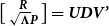 $\big[ \begin{smallmatrix} \textbf{\textit{R}} \\ {\sqrt{\boldsymbol\Lambda}\textbf{\textit{P}}}\end{smallmatrix}\big] = \textbf{\textit{UDV'}}$
be the SVD decomposition. Any rank deficiency is detected at this stage and removed by deleting the corresponding columns from the matrices
$\big[ \begin{smallmatrix} \textbf{\textit{R}} \\ {\sqrt{\boldsymbol\Lambda}\textbf{\textit{P}}}\end{smallmatrix}\big] = \textbf{\textit{UDV'}}$
be the SVD decomposition. Any rank deficiency is detected at this stage and removed by deleting the corresponding columns from the matrices
 $\textbf{\textit{U}}$
and
$\textbf{\textit{U}}$
and
 $\textbf{\textit{V}}$
. Let
$\textbf{\textit{V}}$
. Let
 $\textbf{\textit{U}}_{\bf 1}$
be the submatrix of
$\textbf{\textit{U}}_{\bf 1}$
be the submatrix of
 $\textbf{\textit{U}}$
such that
$\textbf{\textit{U}}$
such that
 $\textbf{\textit{R}} = \textbf{\textit{U}}_{\textbf{\textit{1DV'}}}$
.
$\textbf{\textit{R}} = \textbf{\textit{U}}_{\textbf{\textit{1DV'}}}$
.
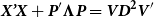 ${\textbf{\textit{X'X}}+\textbf{\textit{P}}'\boldsymbol\Lambda \textbf{\textit{P}}} = \textbf{\textit{VD}}^{\bf 2}\textbf{\textit{V}}'$
and hence the hat matrix
${\textbf{\textit{X'X}}+\textbf{\textit{P}}'\boldsymbol\Lambda \textbf{\textit{P}}} = \textbf{\textit{VD}}^{\bf 2}\textbf{\textit{V}}'$
and hence the hat matrix
 $\textbf{\textit{A}} = \textbf{\textit{X}}(\textbf{\textit{X'X}}+\textbf{\textit{P}}'\boldsymbol\Lambda \textbf{\textit{P}})^{-1}\textbf{\textit{X'}} = \textbf{\textit{QU}}_{\textbf{\textit{1DV'}}}(\textbf{\textit{VD}}^{\bf -2}V')\textbf{\textit{VDU}}_{\bf 1}'\textbf{\textit{Q}}' = \textbf{\textit{QU}}_{\bf 1}\textbf{\textit{U}}_{\bf 1}'\textbf{\textit{Q}}'$
.
$\textbf{\textit{A}} = \textbf{\textit{X}}(\textbf{\textit{X'X}}+\textbf{\textit{P}}'\boldsymbol\Lambda \textbf{\textit{P}})^{-1}\textbf{\textit{X'}} = \textbf{\textit{QU}}_{\textbf{\textit{1DV'}}}(\textbf{\textit{VD}}^{\bf -2}V')\textbf{\textit{VDU}}_{\bf 1}'\textbf{\textit{Q}}' = \textbf{\textit{QU}}_{\bf 1}\textbf{\textit{U}}_{\bf 1}'\textbf{\textit{Q}}'$
.
To guarantee that
 $\lambda_1$
is positive, we parameterise
$\lambda_1$
is positive, we parameterise
 $\lambda_1 = e^{\rho_1}$
. Let
$\lambda_1 = e^{\rho_1}$
. Let
 $\textbf{\textit{G}} = \textbf{\textit{X'X}}+\textbf{\textit{P}}'\boldsymbol\Lambda \textbf{\textit{P}}$
, we have
$\textbf{\textit{G}} = \textbf{\textit{X'X}}+\textbf{\textit{P}}'\boldsymbol\Lambda \textbf{\textit{P}}$
, we have
 \begin{align}\frac{\partial \textbf{\textit{G}}^{\bf -1}}{\partial \rho_1} &= - \textbf{\textit{G}}^{\bf -1} \frac{\partial \textbf{\textit{G}}}{\partial \rho_1} \textbf{\textit{G}}^{\bf -1} \nonumber\\[3pt] &= - \textbf{\textit{G}}^{\bf -1}\textbf{\textit{P'}} \frac{\partial \boldsymbol{\Lambda}}{\partial \rho_1} \textbf{\textit{PG}}^{\bf -1} \nonumber\\[3pt]&= - {\textbf{\textit{G}}^{\bf -1}\textbf{\textit{P}}'\boldsymbol\Lambda \textbf{\textit{PG}}^{\bf -1}} \nonumber\\[3pt] &= - \textbf{\textit{VD}}^{\bf -2}\textbf{\textit{V'P'}}\boldsymbol\Lambda \textbf{\textit{PVD}}^{\bf -2}\textbf{\textit{V'}}\end{align}
and
 \begin{align}\frac{\partial \textbf{\textit{G}}^{\bf -1}}{\partial \lambda_2} &= - \textbf{\textit{G}}^{\bf -1} \frac{\partial \textbf{\textit{G}}}{\partial \lambda_2} \textbf{\textit{G}}^{\bf -1} \nonumber\\[3pt]&= - \textbf{\textit{G}}^{\bf -1}\textbf{\textit{P'}} \frac{\partial \boldsymbol{\Lambda}}{\partial \lambda_2} \boldsymbol{PG}^{\bf -1} \nonumber\\[3pt]&= - \textbf{\textit{G}}^{\bf -1}\textbf{\textit{P'N}}\boldsymbol\Lambda \textbf{\textit{PG}}^{\bf -1}\nonumber\\[3pt]&= - \textbf{\textit{VD}}^{\bf -2}\textbf{\textit{V'P'N}}\boldsymbol\Lambda \textbf{\textit{PVD}}^{\bf -2}\textbf{\textit{V'}}\end{align}
where
 $\textbf{\textit{N}}$
is a diagonal matrix with entries
$\textbf{\textit{N}}$
is a diagonal matrix with entries
 $\textbf{\textit{N}}_{ii} = i$
. In practice we scale the entries
$\textbf{\textit{N}}_{ii} = i$
. In practice we scale the entries
 $\textbf{\textit{N}}_{ii}$
to 0–1 to prevent overflow when
$\textbf{\textit{N}}_{ii}$
to 0–1 to prevent overflow when
 $\lambda_2$
gets huge, as well as the corresponding entries
$\lambda_2$
gets huge, as well as the corresponding entries
 $\boldsymbol{\Lambda}_{ii}$
.
$\boldsymbol{\Lambda}_{ii}$
.
We then have
 \begin{align}\frac{\partial \textbf{\textit{A}}}{\partial \rho_1} &= \frac{\partial \textbf{\textit{XG}}^{\bf -1}\textbf{\textit{X'}}}{\partial \rho_1} \nonumber\\[3pt]&= - \textbf{\textit{X}} \frac{\partial \textbf{\textit{G}}^{\bf -1}}{\partial \rho_1} \textbf{\textit{X'}} \nonumber\\[3pt]&= - \textbf{\textit{XVD}}^{\bf -2}\textbf{\textit{V'P'}}\boldsymbol\Lambda \textbf{\textit{PVD}}^{\bf -2}\textbf{\textit{V'X'}}\nonumber\\[3pt]&= - \textbf{\textit{QU}}_{\textbf{\textit{1DV'VD}}}^{\bf -2}V'P'\Lambda PVD^{-2}\textbf{\textit{V'VDU}}_{\bf 1}'\textbf{\textit{Q}}' \nonumber\\[3pt]&= - {\textbf{\textit{QU}}_{\bf 1}\underbrace{\textbf{\textit{D}}^{\bf -1}\textbf{\textit{V'P'}}\boldsymbol\Lambda \textbf{\textit{PVD}}^{\bf -1}}_{\textbf{\textit{M}}}\textbf{\textit{U}}_{\bf 1}'\textbf{\textit{Q}}'} \nonumber\\[3pt]&= - {\textbf{\textit{QU}}_{\bf1}\textbf{\textit{MU}}_{\bf 1}'\textbf{\textit{Q}}'}\end{align}
and
 \begin{align}\frac{\partial \textbf{\textit{A}}}{\partial \lambda_2} &= \frac{\partial {\textbf{\textit{XG}}^{\bf -1}\textbf{\textit{X}}'}}{\partial \lambda_2}\nonumber\\[3pt] &= - {\textbf{\textit{QU}}_{\bf 1}\underbrace{\textbf{\textit{D}}^{\bf -1}\textbf{\textit{V'P'N}}\boldsymbol\Lambda \textbf{\textit{PVD}}^{\bf -1}}_{\textbf{\textit{M}}^*}\textbf{\textit{U}}_{\bf 1}'\textbf{\textit{Q}}'} \nonumber \\[3pt] &= - {\textbf{\textit{QU}}_{\bf 1}\textbf{\textit{M}}^*\textbf{\textit{U}}_{\bf 1}'\textbf{\textit{Q}}'}\end{align}
Moving on to the Hessian, first we find
 \begin{align}\frac{\partial^2 \textbf{\textit{G}}}{\partial \rho_1\,^2} &= \frac{\partial}{\partial \rho_1} \bigg( \frac{\partial \textbf{\textit{G}}}{\partial \rho_1} \bigg) \nonumber \\[3pt]&= \frac{\partial {\textbf{\textit{P'}}\boldsymbol\Lambda \textbf{\textit{P}}}}{\partial \rho_1} \nonumber \\[3pt]&= {\textbf{\textit{P'}}\boldsymbol\Lambda \textbf{\textit{P}}}\end{align}
so
 \begin{align}\frac{\partial^2 \textbf{\textit{G}}^{\bf -1}}{\partial \rho_1\,^2} &= 2 \, \textbf{\textit{G}}^{\bf -1} \frac{\partial \textbf{\textit{G}}}{\partial \rho_1} \textbf{\textit{G}}^{\bf -1} \frac{\partial \textbf{\textit{G}}}{\partial \rho_1} \textbf{\textit{G}}^{\bf -1} - \textbf{\textit{G}}^{\bf -1} \frac{\partial^2 \textbf{\textit{G}}}{\partial \rho_1 \, ^2} \textbf{\textit{G}}^{\bf -1}\nonumber \\[3pt]&= 2 \, {\textbf{\textit{VD}}^{\bf -2}\textbf{\textit{V'P'}}\boldsymbol\Lambda \textbf{\textit{PVD}}^{\bf -2}\textbf{\textit{V'P'}}\boldsymbol\Lambda \textbf{\textit{PVD}}^{\bf -2}\textbf{\textit{V'}}} {-\textbf{\textit{VD}}^{\bf -2}\textbf{\textit{V'P'}}\boldsymbol\Lambda \textbf{\textit{PVD}}^{\bf -2}\textbf{\textit{V'}}}\end{align}
 \begin{align}\frac{\partial^2 \textbf{\textit{G}}}{\partial \lambda_2\,^2} &= \frac{\partial}{\partial \lambda_2} \bigg( \frac{\partial \textbf{\textit{G}}}{\partial \lambda_2} \bigg) \nonumber \\[3pt]&= \frac{\partial {\textbf{\textit{P'N}}\boldsymbol\Lambda \textbf{\textit{P}}}}{\partial \lambda_2} \nonumber \\[3pt]&= {\textbf{\textit{P'N}}\boldsymbol\Lambda \textbf{\textit{NP}}}\end{align}
so
 \begin{align}\frac{\partial^2 \textbf{\textit{G}}^{\bf -1}}{\partial \lambda_2\,^2} &= 2 \, \textbf{\textit{G}}^{\bf -1} \frac{\partial \textbf{\textit{G}}}{\partial \lambda_2} \textbf{\textit{G}}^{\bf -1} \frac{\partial \textbf{\textit{G}}}{\partial \lambda_2} \textbf{\textit{G}}^{\bf -1} - \textbf{\textit{G}}^{\bf -1} \frac{\partial^2 \textbf{\textit{G}}}{\partial \lambda_2 \, ^2} \textbf{\textit{G}}^{\bf -1}\nonumber \\[3pt]&= 2 \, {\textbf{\textit{VD}}^{\bf -2}\textbf{\textit{V'P'N}}\boldsymbol\Lambda \textbf{\textit{PVD}}^{\bf -2}\textbf{\textit{V'P'N}}\boldsymbol\Lambda \textbf{\textit{PVD}}^{\bf -2}\textbf{\textit{V}}'} \nonumber\\[3pt]&\qquad \qquad \qquad \qquad \qquad \qquad - {\textbf{\textit{VD}}^{\bf -2}\textbf{\textit{V'P'N}}\boldsymbol\Lambda \textbf{\textit{NPVD}}^{\bf -2}\textbf{\textit{V}}'}\end{align}
 \begin{align}\frac{\partial^2 \textbf{\textit{G}}}{\partial \rho_1 \partial \lambda_2} &= \frac{\partial}{\partial \lambda_2} \bigg( \frac{\partial \textbf{\textit{G}}}{\partial \rho_1} \bigg) \nonumber \\[3pt]&= \frac{\partial {\textbf{\textit{P}}'\boldsymbol\Lambda \textbf{\textit{P}}}}{\partial \lambda_2} \nonumber \\[3pt]&= {\textbf{\textit{P'N}}\boldsymbol\Lambda \textbf{\textit{P}}}\end{align}
so
 \begin{align}\frac{\partial^2 \textbf{\textit{G}}^{\bf -1}}{\partial \rho_1 \partial \lambda_2} &= \textbf{\textit{G}}^{\bf -1} \frac{\partial \textbf{\textit{G}}}{\partial \rho_1} \textbf{\textit{G}}^{\bf -1} \frac{\partial \textbf{\textit{G}}}{\partial \lambda_2} \textbf{\textit{G}}^{\bf -1} + \textbf{\textit{G}}^{\bf -1} \frac{\partial \textbf{\textit{G}}}{\partial \lambda_2} \textbf{\textit{G}}^{\bf -1} \frac{\partial \textbf{\textit{G}}}{\partial \rho_1} \textbf{\textit{G}}^{\bf -1} - \textbf{\textit{G}}^{\bf -1} \frac{\partial^2 \textbf{\textit{G}}}{\partial \rho_1 \partial \lambda_2} \textbf{\textit{G}}^{\bf -1}\nonumber\\[3pt]&= {\textbf{\textit{VD}}^{\bf -2}\textbf{\textit{V'P'}}\boldsymbol\Lambda \textbf{\textit{PVD}}^{\bf -2}\textbf{\textit{V'P'N}}\boldsymbol\Lambda \textbf{\textit{PVD}}^{\bf -2}\textbf{\textit{V'}}} \nonumber\\[3pt]& \qquad {\boldsymbol+ \textbf{\textit{VD}}^{\bf -2}\textbf{\textit{V'P'N}}\boldsymbol\Lambda \textbf{\textit{PVD}}^{\bf -2}\textbf{\textit{V'P'}}\boldsymbol\Lambda \textbf{\textit{PVD}}^{\bf -2}\textbf{\textit{V'}}} {- \textbf{\textit{VD}}^{\bf -2}\textbf{\textit{V'P'N}}\boldsymbol\Lambda \textbf{\textit{PVD}}^{\bf -2}\textbf{\textit{V'}}}\end{align}
Therefore,
 \begin{align}\frac{\partial^2 \textbf{\textit{A}}}{\partial \rho_1 \, ^2} &= \textbf{\textit{X}} \frac{\partial^2 \textbf{\textit{G}}^{\bf -1}}{\partial \rho_1 \, ^2} \textbf{\textit{X'}} \nonumber \\[3pt]&= {\textbf{\textit{QU}}_{\bf 1}\textbf{\textit{DV'}}} (2 \, {\textbf{\textit{VD}}^{\bf -2}\textbf{\textit{V'P'}}\boldsymbol\Lambda \textbf{\textit{PVD}}^{\bf -2}\textbf{\textit{V'P'}}\boldsymbol\Lambda \textbf{\textit{PVD}}^{\bf -2}\textbf{\textit{V}}'} \nonumber\\[3pt]&\qquad \qquad \qquad \qquad \qquad \qquad - {\textbf{\textit{VD}}^{\bf -2}\textbf{\textit{V'P'}}\boldsymbol\Lambda \textbf{\textit{PVD}}^{\bf -2}\textbf{\textit{V'}}}) {\textbf{\textit{VDU}}_{\bf 1}'\textbf{\textit{Q}}'} \nonumber \\[3pt]&= 2\, {\textbf{\textit{QU}}_{\bf 1}\textbf{\textit{MMU}}_{\bf 1}'\textbf{\textit{Q}}'} - {\textbf{\textit{QU}}_{\bf 1}\textbf{\textit{MU}}_{\bf 1}'\textbf{\textit{Q}}'} \nonumber \\[3pt]&= 2\, {\textbf{\textit{QU}}_{\bf 1}\textbf{\textit{MMU}}_{\bf 1}'\textbf{\textit{Q}}'} + \frac{\partial \textbf{\textit{A}}}{\partial \rho_1}\end{align}
 \begin{align}\frac{\partial^2 \textbf{\textit{A}}}{\partial \lambda_2 \, ^2} &= \textbf{\textit{X}} \frac{\partial^2 \textbf{\textit{G}}^{\bf -1}}{\partial \lambda_2 \, ^2} \textbf{\textit{X'}} \nonumber \\[3pt]&= {\textbf{\textit{QU}}_{\bf 1}\textbf{\textit{DV}}'} (2 \, {\textbf{\textit{VD}}^{\bf -2}\textbf{\textit{V'P'N}}\boldsymbol\Lambda \textbf{\textit{PVD}}^{\bf -2}\textbf{\textit{V'P'N}}\boldsymbol\Lambda \textbf{\textit{PVD}}^{\bf -2}\textbf{\textit{V'}}} \nonumber\\[3pt]&\qquad \qquad \qquad \qquad \qquad \qquad - {\textbf{\textit{VD}}^{\bf -2}\textbf{\textit{V'P'N}}\boldsymbol\Lambda \textbf{\textit{NPVD}}^{\bf -2}\textbf{\textit{V'}}}) {\textbf{\textit{VDU}}_{\bf 1}'\textbf{\textit{Q}}'} \nonumber \\[3pt]&= 2\, {\textbf{\textit{QU}}_{\bf 1}\textbf{\textit{M}}^*\textbf{\textit{M}}^*\textbf{\textit{U}}_{\bf 1}'\textbf{\textit{Q}}'} - {\textbf{\textit{QU}}_{\bf 1}\underbrace{\textbf{\textit{D}}^{\bf -1}\textbf{\textit{V'P'N}}\boldsymbol\Lambda \textbf{\textit{NPVD}}^{\bf -1}}_{\textbf{\textit{M}}^{\bf **}}\textbf{\textit{U}}_{\bf 1}'\textbf{\textit{Q}}'} \nonumber \\[3pt]&= 2\, {\textbf{\textit{QU}}_{\bf 1}\textbf{\textit{M}}^*\textbf{\textit{M}}^*\textbf{\textit{U}}_{\bf 1}'\textbf{\textit{Q}}' - \textbf{\textit{QU}}_{\bf 1}\textbf{\textit{M}}^{**}\textbf{\textit{U}}_{\bf 1}'\textbf{\textit{Q}}'}\end{align}
and
 \begin{align}\frac{\partial^2 \textbf{\textit{A}}}{\partial \rho_1 \partial \lambda_2} &= \textbf{\textit{X}} \frac{\partial^2 \textbf{\textit{G}}^{\bf -1}}{\partial \rho_1 \partial \lambda_2 } \textbf{\textit{X'}} \nonumber \\[3pt]&= {\textbf{\textit{QU}}_{\bf 1}\textbf{\textit{MM}}^*\textbf{\textit{U}}_{\bf 1}'\textbf{\textit{Q}}' + \textbf{\textit{QU}}_{\bf 1} \textbf{\textit{M}}^*\textbf{\textit{MU}}_{\bf 1}'\textbf{\textit{Q}}' - \textbf{\textit{QU}}_{\bf 1}\textbf{\textit{M}}^*\textbf{\textit{U}}_{\bf 1}'\textbf{\textit{Q}}'} \nonumber \\[3pt]&= {\textbf{\textit{QU}}_{\bf 1}\textbf{\textit{MM}}^*\textbf{\textit{U}}_{\bf 1}'\textbf{\textit{Q}}' + \textbf{\textit{QU}}_{\bf 1} \textbf{\textit{M}}^*\textbf{\textit{MU}}_{\bf 1}'\textbf{\textit{Q}}'} + \frac{\partial \textbf{\textit{A}}}{\partial \lambda_2}\end{align}
Finally, the BIC for is
 $-2\log(L) + \log(n) \, \textrm{rm} (\textbf{\textit{A}})$
, where L is the maximum likelihood.
$-2\log(L) + \log(n) \, \textrm{rm} (\textbf{\textit{A}})$
, where L is the maximum likelihood.
 \begin{align}\frac{\partial \tilde{\sigma}^2}{\partial \rho_1} &= - \frac{2}{n} \, (\textbf{\textit{y}}-\textbf{\textit{Ay}})' \, \frac{\partial \textbf{\textit{A}}}{\partial \rho_1} \, \textbf{\textit{y}} \qquad \text{and} \qquad \frac{\partial \tilde{\sigma}^2}{\partial \lambda_2} = - \frac{2}{n} \, (\textbf{\textit{y}}-\textbf{\textit{Ay}})' \, \frac{\partial \textbf{\textit{A}}}{\partial \lambda_2} \, \textbf{\textit{y}}\end{align}
 \begin{align}\frac{\partial^2 \tilde{\sigma}^2}{\partial \rho_1 \, ^2} &= -\frac{2}{n} \left[ (\textbf{\textit{y}}-\textbf{\textit{Ay}})' \, \frac{\partial^2 \textbf{\textit{A}}}{\partial \rho_1 \, ^2} \, \textbf{\textit{y}} - \textbf{\textit{y}}' \bigg(\frac{\partial \textbf{\textit{A}}}{\partial \rho_1}\bigg)\bigg(\frac{\partial \textbf{\textit{A}}}{\partial \rho_1}\bigg) \textbf{\textit{y}}\right] \nonumber\\[3pt] \frac{\partial^2 \tilde{\sigma}^2}{\partial \lambda_2 \, ^2} &= -\frac{2}{n} \left[ (\textbf{\textit{y}}-\textbf{\textit{Ay}})' \, \frac{\partial^2 \textbf{\textit{A}}}{\partial \lambda_2 \, ^2} \, \textbf{\textit{y}} - \textbf{\textit{y}}' \bigg(\frac{\partial \textbf{\textit{A}}}{\partial \lambda_2}\bigg)\bigg(\frac{\partial \textbf{\textit{A}}}{\partial \lambda_2}\bigg) \textbf{\textit{y}}\right] \qquad \text{and} \nonumber\\[3pt] \frac{\partial^2 \tilde{\sigma}^2}{\partial \rho_1 \partial \lambda_2} &= -\frac{2}{n} \left[ (\textbf{\textit{y}}-\textbf{\textit{Ay}})' \, \frac{\partial^2 \textbf{\textit{A}}}{\partial \rho_1 \partial \lambda_2} \, \textbf{\textit{y}} - \textbf{\textit{y}}' \bigg(\frac{\partial \textbf{\textit{A}}}{\partial \rho_1}\bigg)\bigg(\frac{\partial \textbf{\textit{A}}}{\partial \lambda_2}\bigg) \textbf{\textit{y}}\right] \end{align}
 \begin{align}\frac{\partial BIC}{\partial \rho_1} &= \frac{n}{\tilde{\sigma}^2} \, \frac{\partial \tilde{\sigma}^2}{\partial \rho_1} + \log (n) \textrm{rm} \bigg( \frac{\partial \textbf{\textit{A}}}{\partial \rho_1} \bigg)\end{align}
Similarly,
 \begin{align}\frac{\partial BIC}{\partial \lambda_2} &= \frac{n}{\tilde{\sigma}^2} \, \frac{\partial \tilde{\sigma}^2}{\partial \lambda_2} + \log (n) \textrm{rm} \bigg( \frac{\partial \textbf{\textit{A}}}{\partial \lambda_2} \bigg)\end{align}
 \begin{align}\frac{\partial^2 BIC}{\partial \rho_1 \, ^2} &= n \bigg[ \frac{1}{\tilde{\sigma}^2} \, \frac{\partial^2 \tilde{\sigma}^2}{\partial \rho_1 \, ^2} - \frac{1}{\tilde{\sigma}^4} \bigg( \frac{\partial \tilde{\sigma}^2}{\partial \rho_1}\bigg)^2\bigg] + \log (n) \, \textrm{rm} \bigg( \frac{\partial^2 \textbf{\textit{A}}}{\partial \rho_1\,^2}\bigg)\end{align}
 \begin{align}\frac{\partial^2 BIC}{\partial \lambda_2 \, ^2} &= n \bigg[ \frac{1}{\tilde{\sigma}^2} \, \frac{\partial^2 \tilde{\sigma}^2}{\partial \lambda_2 \, ^2} - \frac{1}{\tilde{\sigma}^4} \bigg( \frac{\partial \tilde{\sigma}^2}{\partial \lambda_2}\bigg)^2\bigg] + \log (n) \, \textrm{rm} \bigg( \frac{\partial^2 \textbf{\textit{A}}}{\partial \lambda_2\,^2}\bigg)\end{align}
and
 \begin{align}\frac{\partial^2 BIC}{\partial \rho_1 \partial \lambda_2} &= n \bigg[ \frac{1}{\tilde{\sigma}^2} \, \frac{\partial^2 \tilde{\sigma}^2}{\partial \rho_1 \partial \lambda_2} - \frac{1}{\tilde{\sigma}^4} \bigg( \frac{\partial \tilde{\sigma}^2}{\partial \rho_1}\bigg)\bigg( \frac{\partial \tilde{\sigma}^2}{\partial \lambda_2}\bigg)\bigg] + \log (n) \, \textrm{rm} \bigg( \frac{\partial^2 \textbf{\textit{A}}}{\partial \rho_1 \partial \lambda_2}\bigg)\end{align}
As mentioned, for non-Gaussian data, optimisation can be performed within each P-IRLS iteration and is done simply by replacing the design matrix and data with
 $\sqrt{\textbf{\textit{W}}} \textbf{\textit{X}}$
and
$\sqrt{\textbf{\textit{W}}} \textbf{\textit{X}}$
and
 $\sqrt{\textbf{\textit{W}}} \textbf{\textit{z}}$
, respectively, where
$\sqrt{\textbf{\textit{W}}} \textbf{\textit{z}}$
, respectively, where
 $\textbf{\textit{W}}$
is a diagonal matrix with the current working weights and
$\textbf{\textit{W}}$
is a diagonal matrix with the current working weights and
 $\textbf{\textit{z}}$
is the vector of working pseudo-data.
$\textbf{\textit{z}}$
is the vector of working pseudo-data.
Appendix B. Gradient and Hessian for the Newton–Raphson of the Joint Model
Recall that the penalty matrix for the joint model is
 $\bigg(\begin{smallmatrix} {\sqrt{\boldsymbol\Lambda^{\textbf{\textit{M}}}} \textbf{\textit{P}}^{\textbf{\textit{M}}}} \\ {\sqrt{\boldsymbol\Lambda^{\textbf{\textit{F}}}} \textbf{\textit{P}}^{\textbf{\textit{F}}}} \\ {\sqrt{\boldsymbol\Lambda^{\textbf{\textit{D}}}} \textbf{\textit{P}}^\textbf{\textit{D}}}\end{smallmatrix}\bigg)$
. Similarly to constraint
$\bigg(\begin{smallmatrix} {\sqrt{\boldsymbol\Lambda^{\textbf{\textit{M}}}} \textbf{\textit{P}}^{\textbf{\textit{M}}}} \\ {\sqrt{\boldsymbol\Lambda^{\textbf{\textit{F}}}} \textbf{\textit{P}}^{\textbf{\textit{F}}}} \\ {\sqrt{\boldsymbol\Lambda^{\textbf{\textit{D}}}} \textbf{\textit{P}}^\textbf{\textit{D}}}\end{smallmatrix}\bigg)$
. Similarly to constraint
 $\lambda^M_1, \lambda^F_1$
and
$\lambda^M_1, \lambda^F_1$
and
 $\lambda^D_1$
to be strictly positive, they are re-parameterised to
$\lambda^D_1$
to be strictly positive, they are re-parameterised to
 $\lambda^j_1 = e^{\, \rho^j_1}$
and the gradients with respect to
$\lambda^j_1 = e^{\, \rho^j_1}$
and the gradients with respect to
 $(\rho^j_1)$
are simply found by replacing
$(\rho^j_1)$
are simply found by replacing
 $\textbf{\textit{P}}$
and
$\textbf{\textit{P}}$
and
 $\boldsymbol{\Lambda}$
in derivatives equations (A.1)–(A.20) by the corresponding
$\boldsymbol{\Lambda}$
in derivatives equations (A.1)–(A.20) by the corresponding
 ${\textbf{\textit{P}}^{\textbf{\textit{j}}}}$
and
${\textbf{\textit{P}}^{\textbf{\textit{j}}}}$
and
 $\boldsymbol{\Lambda}^{\textbf{\textit{j}}}$
. For example,
$\boldsymbol{\Lambda}^{\textbf{\textit{j}}}$
. For example,
 \begin{align}\frac{\partial \textbf{\textit{A}}}{\partial \rho^M_1} = -&{\textbf{\textit{QU}}_{\bf 1}\textbf{\textit{M}}^{\textbf{\textit{M}}}\textbf{\textit{U}}_{\bf 1}^{\prime}\textbf{\textit{Q}}^{\boldsymbol\prime}} \quad \text{and} \quad \frac{\partial \textbf{\textit{A}}}{\partial \rho^D_1} = -{\textbf{\textit{QU}}_{\bf 1}\textbf{\textit{M}}^{\textbf{\textit{D}}}\textbf{\textit{U}}_{\bf 1}'\textbf{\textit{Q}}'} \nonumber\\\text{where} \, &{\textbf{\textit{M}}^{\textbf{\textit{j}}}} = {\textbf{\textit{D}}^{\bf -1}\textbf{\textit{V}}^{\prime}\textbf{\textit{P}}^{\textbf{\textit{j}}\prime}\boldsymbol\Lambda^{\textbf{\textit{j}}}\textbf{\textit{P}}^{\textbf{\textit{j}}}\textbf{\textit{VD}}^{\bf -1}}\end{align}
The Hessian requires a little more attention and slight adjustments have to be made. We have,
 \begin{align}\frac{\partial^2 \textbf{\textit{A}}}{\partial \rho^i_1 \partial \rho^j_1} &= {\textbf{\textit{QU}}_{\bf 1}\textbf{\textit{M}}^{\textbf{\textit{i}}}\textbf{\textit{M}}^{\textbf{\textit{j}}}\textbf{\textit{U}}_{\bf 1}^{\boldsymbol{\prime}}\textbf{\textit{Q}}^{\boldsymbol\prime} + \textbf{\textit{QU}}_{\bf 1} \textbf{\textit{M}}^{\textbf{\textit{j}}}\textbf{\textit{M}}^{\textbf{\textit{i}}}\textbf{\textit{U}}_{\bf 1}^{\boldsymbol\prime}\textbf{\textit{Q}}^{\prime}} - \delta_{ij} \, {\textbf{\textit{QU}}_{\bf 1}\textbf{\textit{M}}^{\textbf{\textit{j}}}\textbf{\textit{U}}_{\bf 1}^{\prime}\textbf{\textit{Q}}^{\prime}} \nonumber\\[3pt]&= {\textbf{\textit{QU}}_{\bf 1}\textbf{\textit{M}}^{\textbf{\textit{i}}}\textbf{\textit{M}}^{\textbf{\textit{j}}}\textbf{\textit{U}}_{\bf 1}^{\prime}\textbf{\textit{Q}}^{\prime} + \textbf{\textit{QU}}_{\bf 1} \textbf{\textit{M}}^{\textbf{\textit{j}}}\textbf{\textit{M}}^{\textbf{\textit{i}}}\textbf{\textit{U}}_{\bf 1}^{\prime}\textbf{\textit{Q}}^{\prime}} + \delta_{ij} \, \frac{\partial \textbf{\textit{A}}}{\partial \rho^j_1}\end{align}
 \begin{align}\frac{\partial^2 \textbf{\textit{A}}}{\partial \lambda^i_2 \partial \lambda^j_2} &= {\textbf{\textit{QU}}_{\bf 1}\textbf{\textit{M}}^{*^i}\textbf{\textit{M}}^{*^{\textbf{\textit{j}}}}\textbf{\textit{U}}_{\bf 1}^{\prime}\textbf{\textit{Q}}^{\prime} + \textbf{\textit{QU}}_{\bf 1} \textbf{\textit{M}}^{*^j}\textbf{\textit{M}}^{*^{\textbf{\textit{i}}}}\textbf{\textit{U}}_{\bf 1}^{\prime}\textbf{\textit{Q}}^{\prime}} - \delta_{ij} \, {\textbf{\textit{QU}}_{\bf 1}\textbf{\textit{M}}^{**^{\textbf{\textit{j}}}}\textbf{\textit{U}}_{\bf 1}^{\prime}\textbf{\textit{Q}}^{\prime}}\end{align}
 \begin{align}\frac{\partial^2 \textbf{\textit{A}}}{\partial \rho^i_1 \partial \lambda^j_2} &= {\textbf{\textit{QU}}_{\bf 1}\textbf{\textit{M}}^{\textbf{\textit{i}}}\textbf{\textit{M}}^{*^{\textbf{\textit{j}}}}\textbf{\textit{U}}_{\bf 1}^{\prime}\textbf{\textit{Q}}^{\prime} + \textbf{\textit{QU}}_{\bf 1} \textbf{\textit{M}}^{*^{\textbf{\textit{j}}}}\textbf{\textit{M}}^{\textbf{\textit{i}}}\textbf{\textit{U}}_{\bf 1}^{\boldsymbol\prime}\textbf{\textit{Q}}^{\boldsymbol\prime}} - \delta_{ij} \, {\textbf{\textit{QU}}_{\bf 1}\textbf{\textit{M}}^{*^{\textbf{\textit{j}}}}\textbf{\textit{U}}_{\bf 1}^{\prime}\textbf{\textit{Q}}^{\prime}} \nonumber\\[3pt]&= {\textbf{\textit{QU}}_{\bf 1}\textbf{\textit{M}}^{\textbf{\textit{i}}}\textbf{\textit{M}}^{*^{\textbf{\textit{j}}}}\textbf{\textit{U}}_{\bf 1}^{\prime}\textbf{\textit{Q}}^{\boldsymbol\prime} + \textbf{\textit{QU}}_{\bf 1} \textbf{\textit{M}}^{*^{\textbf{\textit{j}}}}\textbf{\textit{M}}^{\textbf{\textit{i}}}\textbf{\textit{U}}_{\bf 1}^{\prime}\textbf{\textit{Q}}^{\boldsymbol\prime}} + \delta_{ij} \, \frac{\partial \textbf{\textit{A}}}{\partial \lambda^j_2}\end{align}
where
 $\delta_{ij}$
is the Kronecker delta function.
$\delta_{ij}$
is the Kronecker delta function.


 Open access