2 Derivation of fourth-order NSE from ZIE

The governing equations for an inviscid, incompressible fluid of infinite depth with a free surface under the influence of both gravity and surface tension are

(2.1) $$ \begin{align} & \frac{\partial^{2}\phi}{\partial x^{2}}+ \frac{\partial^{2}\phi}{\partial z^{2}}=0, \quad \frac{\partial^{2}\psi}{\partial x^{2}}+ \frac{\partial^{2}\psi}{\partial z^{2}}=0, \quad -\infty<z<\eta , \end{align} $$

(2.2) $$ \begin{align} & \frac{\partial\phi}{\partial z}- \frac{\partial\eta}{\partial t}=\bigg( \frac{\partial\phi}{\partial x}+\Omega\eta\bigg) \frac{\partial\eta}{\partial x}, \quad z=\eta, \end{align} $$

(2.3) $$ \begin{align} & \frac{\partial\phi}{\partial t}-\Omega\psi+g\eta=-\frac{1}{2}\bigg\{\bigg(\frac{\partial\phi}{\partial x}\bigg)^{2}+\bigg(\frac{\partial\phi}{\partial z}\bigg)^{2} \bigg\}-\Omega\eta \frac{\partial\phi}{\partial x} +\bigg(\frac{{T}}{\rho}\bigg) \frac{\partial^{2}\eta}{\partial x^{2}}\bigg\{1+\bigg(\frac{\partial\eta}{\partial x}\bigg)^{2}\bigg\}^{-3/2}, \quad z=\eta, \end{align} $$

(2.4) $$ \begin{align} & \phi,\psi\rightarrow0,\quad z=-\infty, \end{align} $$

where $\Omega $ is the magnitude of the shear, ${T}$ is the surface tension coefficient, $\phi (x,z,t)$ is the velocity potential, $\psi (x,z,t)$ is the stream function and the last two functions are related by the Cauchy–Riemann equations

(2.5) $$ \begin{align} \frac{\partial\phi}{\partial x}=\frac{\partial\psi}{\partial z},\quad \frac{\partial\phi}{\partial z} =-\frac{\partial\psi}{\partial x}. \end{align} $$

The basic flow of interest is a constant shear current given by $v(z)$ = $\Omega z$ . The fluid velocity can then be expressed as $\textbf {u}(x,z)$ = $\Omega z \hat {i} + \nabla \phi (x,z,t)$ , where $\nabla \phi (x,z,t)$ is the wave-induced velocity. The waves are potentially due to the Kelvin theorem which states that vorticity is conserved for a two-dimensional flow of an incompressible fluid with external forces derived from a potential.

Linearizing (2.2), (2.3), and using (2.1), (2.4) and (2.5), the dispersion relation determining $\omega $ is given by

$$ \begin{align*} \omega^{2}+\omega\Omega-g|{\boldsymbol{k}}|\bigg(1+\frac{{T}|{\boldsymbol{k}}|^{2}}{\rho g}\bigg)=0. \end{align*} $$

Zakharov [Reference Zakharov44] showed that the governing equation for nonlinear periodic waves in deep water accurate to third-order in amplitude is

(2.6) $$ \begin{align} i\frac{\partial H}{\partial t}({\boldsymbol{k}},t)&=\int^\infty _{-\infty}[S({\boldsymbol{k}},{\boldsymbol{k}}_{1},{\boldsymbol{k}}_{2},{\boldsymbol{k}}_{3})H^{\ast}({\boldsymbol{k}}_{1},t)H({\boldsymbol{k}}_{2},t)H({\boldsymbol{k}}_{3},t)\delta({\boldsymbol{k}}+{\boldsymbol{k}}_{1}-{\boldsymbol{k}}_{2}-{\boldsymbol{k}}_{3}) \nonumber \\ & \quad \times {e}^{i\{\omega({\boldsymbol{k}})+\omega({\boldsymbol{k}}_{1})-\omega({\boldsymbol{k}}_{2})-\omega({\boldsymbol{k}}_{3}) \}}]\,{d}{\boldsymbol{k}}_{1}\,{d}{\boldsymbol{k}}_{2}\,{d}{\boldsymbol{k}}_{3}, \end{align} $$

where $H({\boldsymbol {k}},t)$ can be taken as the component of the wave envelope that is connected to the surface elevation

(2.7) $$ \begin{align} \eta({\boldsymbol{x}},t)=\frac{1}{2\pi}\int^\infty _{-\infty}\bigg(\frac{| {\boldsymbol{k}} | }{2\omega({\boldsymbol{k}})} \bigg)^{1/2}[H({\boldsymbol{k}},t) e^ {i\{ {\boldsymbol{k}}.{\boldsymbol{x}}-\omega({\boldsymbol{k}}) t \}}+\text{c}.\text{c}.]\,{d}{\boldsymbol{k}}, \end{align} $$

where ${\boldsymbol {k}}=(k,l)$ is the wave vector, $(x,y)={\boldsymbol {x}}$ are the horizontal coordinates and c.c. represents the complex conjugate. The interaction coefficient $S({\boldsymbol {k}},{\boldsymbol {k}}_{1},{\boldsymbol {k}}_{2},{\boldsymbol {k}}_{3})$ is a real function and was provided for a free surface CGW by Zakharov [Reference Zakharov44]. The accurate form of Zakharov’s kernel was given by Hogan [Reference Hogan17] for CGWs using the simplified notation of Crawford et al. [Reference Crawford, Lake, Saffman and Yuen7]. In this paper, we have used the expression for $S({\boldsymbol {k}},{\boldsymbol {k}}_{1},{\boldsymbol {k}}_{2},{\boldsymbol {k}}_{3})$ provided by Hogan [Reference Hogan17].

The frequency $\omega ({\boldsymbol {k}})$ of the CGW is

$$ \begin{align*} \omega({\boldsymbol{k}})=-\frac{\Omega}{2}+\bigg\{\frac{\Omega^{2}}{4}+g|{\boldsymbol{k}}|(1+\nu) \bigg\}^{1/2}, \end{align*} $$

where $\nu ={{T}|{\boldsymbol {k}}|^{2}}/{\rho g}$ . Herein, like Stiassnie [Reference Stiassnie39], the fourth-order NSE for a group of CGWs is developed from (2.6). We take a narrow spectrum centred on ${\boldsymbol {k}}_{0}=(k_{0},0)$ , and set

$$ \begin{align*} {\boldsymbol{k}}={\boldsymbol{k}}_{0}+{\boldsymbol{\lambda}}\quad \text{and} \quad {\boldsymbol{k}}_{n}={\boldsymbol{k}}_{0}+{\boldsymbol{\lambda}}_{n},\quad {\boldsymbol{\lambda}}=\lambda\hat{i}, \quad n=1,2,3, \end{align*} $$

where the measure of the spectral bandwidth is taken as ${|{\boldsymbol {\lambda }}|}/{k_{0}},{|{\boldsymbol {\lambda }}_{n}|}/{k_{0}}=O(1)$ .

Defining a variable given by

$$ \begin{align*} F({\boldsymbol{\lambda}},t)=H({\boldsymbol{k}},t) e^{-i\{\omega({\boldsymbol{k}})-\omega({\boldsymbol{k}}_{0})\}t}, \end{align*} $$

and inserting this in (2.6) and (2.7),

(2.8) $$ \begin{align} i\frac{\partial F}{\partial t}({\boldsymbol{\lambda}},t)-\{\omega({\boldsymbol{k}})-\omega({\boldsymbol{k}}_{0})\}F({\boldsymbol{\lambda}},t) &=\int^\infty _{-\infty}[S({\boldsymbol{k}}_{0}+{\boldsymbol{\lambda}},{\boldsymbol{k}}_{0}+{\boldsymbol{\lambda}}_{1},{\boldsymbol{k}}_{0}+{\boldsymbol{\lambda}}_{2},{\boldsymbol{k}}_{0}+{\boldsymbol{\lambda}}_{3}) F^{\ast}({\boldsymbol{\lambda}}_{1},t) \nonumber \\ &\quad \times F({\boldsymbol{\lambda}}_{2},t)F({\boldsymbol{\lambda}}_{3},t)\delta({\boldsymbol{\lambda}}+{\boldsymbol{\lambda}}_{1}-{\boldsymbol{\lambda}}_{2}-{\boldsymbol{\lambda}}_{3})]\,{d}{\boldsymbol{\lambda}}_{1}\,{d}{\boldsymbol{\lambda}}_{2}\,{d}{\boldsymbol{\lambda}}_{3}, \end{align} $$

(2.9) $$ \begin{align} \eta({\boldsymbol{x}},t)=\frac{1}{2\pi}\sqrt{\frac{k_{0}}{2\omega(k_{0})}} e^ {i\{ {\boldsymbol{k}}_{0}.{\boldsymbol{x}}-\omega({\boldsymbol{k}}_{0}) t \}}&\int^\infty _{-\infty}\{(1+u\lambda/k_{0})F({\boldsymbol{\lambda}},t) e ^{(i{\boldsymbol{\lambda}}.{\boldsymbol{x}})}+\text{c}.\text{c}.\}\,{d}{\boldsymbol{\lambda}}, \end{align} $$

in which u appearing in (2.9) is shown in Appendix A.

We now rewrite (2.9) as

$$ \begin{align*} \eta({\boldsymbol{x}},t)=\tfrac{1}{2}[a({\boldsymbol{x}},t) e ^{i\{ {\boldsymbol{k}}_{0}.{\boldsymbol{x}}-\omega({\boldsymbol{k}}_{0}) t \}}+c.c.], \end{align*} $$

where

$$ \begin{align*} a({\boldsymbol{x}},t)=\frac{1}{2\pi}\sqrt{\frac{k_{0}}{2\omega(k_{0})}}\int^\infty _{-\infty}\{(1+u\lambda/k_{0})F({\boldsymbol{\lambda}},t) e ^{(i{\boldsymbol{\lambda}}.{\boldsymbol{x}})}+\text{c}.\text{c}.\}\,{d}{\boldsymbol{\lambda}}. \end{align*} $$

The expression for frequency difference $\omega ({\boldsymbol {k}}_{0}+{\boldsymbol {\lambda }})-\omega ({\boldsymbol {k}}_{0})$ of (2.8) can be expressed by the Taylor series expansion in different powers of spectral width given by

(2.10) $$ \begin{align} \omega({\boldsymbol{k}}_{0}+{\boldsymbol{\lambda}})-\omega({\boldsymbol{k}}_{0})=\omega({\boldsymbol{k}}_{0})\bigg[\gamma_{1}\frac{\lambda}{k_0}-\gamma_{2}\frac{\lambda^2}{k_0^{2}}+\gamma_{3}\frac{\lambda^3}{k_0^{3}} \bigg]. \end{align} $$

We insert (2.10) in (2.8), multiply by $\sqrt {{k_{0}}/{2\omega (k_{0})}}\,\big (1+u\lambda /k_{0}\big )/2\pi $ and then take the inverse Fourier transform to get

(2.11) $$ \begin{align} & i\frac{\partial a}{\partial t}({\boldsymbol{x}},t)-\frac{1}{2\pi}\int^\infty _{-\infty}\{\omega({\boldsymbol{k}}_{0}+{\boldsymbol{\lambda}})-\omega({\boldsymbol{k}}_{0})\} a({\boldsymbol{\lambda}},t) e^{(i{\boldsymbol{\lambda}}.{\boldsymbol{x}})}\,{d}{\boldsymbol{\lambda}} \nonumber \\ &\quad =\frac{\omega(k_{0})}{4\pi k_0}\int^\infty _{-\infty}[S({\boldsymbol{k}}_{0}+{\boldsymbol{\lambda}}_{2}+{\boldsymbol{\lambda}}_{3}-{\boldsymbol{\lambda}}_{1},{\boldsymbol{k}}_{0}+{\boldsymbol{\lambda}}_{1},{\boldsymbol{k}}_{0}+{\boldsymbol{\lambda}}_{2},{\boldsymbol{k}}_{0}+{\boldsymbol{\lambda}}_{3}) \nonumber \\ &\qquad \times[1+u(\lambda_{2}+\lambda_{3}-\lambda_{1})/k_0 ][1-u\lambda_{1}/k_0 ][1-u\lambda_{2}/k_0 ][1-u\lambda_{3}/k_0 ] \nonumber \\ & \qquad \times a^{\ast}({\boldsymbol{\lambda}}_{1},t) a({\boldsymbol{\lambda}}_{2},t) a({\boldsymbol{\lambda}}_{3},t) e^{[{i({\boldsymbol{\lambda}}_{2}+{\boldsymbol{\lambda}}_{3}-{\boldsymbol{\lambda}}_{1}).{\boldsymbol{x}}}]}]\,{d}{\boldsymbol{\lambda}}_{1}\,{d}{\boldsymbol{\lambda}}_{2}\,{d}{\boldsymbol{\lambda}}_{3}. \end{align} $$

For evaluating the triple integral of (2.11), we need the following Taylor series expansion of S, accurate to first order in the spectral bandwidth

(2.12) $$ \begin{align} &S({\boldsymbol{k}}_{0}+{\boldsymbol{\lambda}}_{2}+{\boldsymbol{\lambda}}_{3}-{\boldsymbol{\lambda}}_{1},{\boldsymbol{k}}_{0}+{\boldsymbol{\lambda}}_{1},{\boldsymbol{k}}_{0}+{\boldsymbol{\lambda}}_{2},{\boldsymbol{k}}_{0}+{\boldsymbol{\lambda}}_{3}) \nonumber\\& \quad =\frac{k_0^{3}}{8\pi^{2}}\bigg[\mu_{1}-\mu_{2}\frac{(\lambda_{2}+\lambda_{3})}{k_0}+\mu{'}_{3}\frac{\lambda_{1}}{k_0}-\frac{\mu_{4}}{k_0}\bigg\{\frac{({\boldsymbol{\lambda}}_{3}-{\boldsymbol{\lambda}}_{1})^2}{| {\boldsymbol{\lambda}}_{3}-{\boldsymbol{\lambda}}_{1}|}+\frac{({\boldsymbol{\lambda}}_{2}-{\boldsymbol{\lambda}}_{1})^2}{| {\boldsymbol{\lambda}}_{2}-{\boldsymbol{\lambda}}_{1} |} \bigg\} \bigg]. \end{align} $$

Substituting (2.12) and (2.10) in (2.11),

$$ \begin{align*} i\frac{\partial a}{\partial t}({\boldsymbol{x}},t) &-\frac{\omega(k_0)}{2\pi}\int^\infty _{-\infty}\bigg[\gamma_{1}\frac{\lambda}{k_0}-\gamma_{2}\frac{\lambda^2}{k_0^{2}}+\gamma_{3}\frac{\chi^3}{k_0^{3}}\bigg] a({\boldsymbol{\lambda}},t)e^{(i{\boldsymbol{\lambda}}.{\boldsymbol{x}})}\,{d}{\boldsymbol{\lambda}} \nonumber \\ & =\frac{k_0^{2}\omega(k_{0})}{32\pi^3}\int^\infty _{-\infty}\bigg[\bigg\{\mu_{1}-\mu_{2}\frac{(\lambda_{2}+\lambda_{3})}{k_0}+\mu_{3}\frac{\lambda_{1}}{k_0}-\frac{\mu_{4}}{k_0}\bigg(\frac{({\boldsymbol{\lambda}}_{3}-{\boldsymbol{\lambda}}_{1})^2}{| {\boldsymbol{\lambda}}_{3}-{\boldsymbol{\lambda}}_{1} |} +\frac{({\boldsymbol{\lambda}}_{2}-{\boldsymbol{\lambda}}_{1})^2}{| {\boldsymbol{\lambda}}_{2}-{\boldsymbol{\lambda}}_{1} |} \bigg)\bigg\} \nonumber \\ & \quad \times a^{\ast}({\boldsymbol{\lambda}}_{1},t) a({\boldsymbol{\lambda}}_{2},t) a({\boldsymbol{\lambda}}_{3},t)e^{{i({\boldsymbol{\lambda}}_{2}+{\boldsymbol{\lambda}}_{3}-{\boldsymbol{\lambda}}_{1}).{\boldsymbol{x}}}}\bigg]\,{d}{\boldsymbol{\lambda}}_{1}\,{d}{\boldsymbol{\lambda}}_{2}\,{d}{\boldsymbol{\lambda}}_{3}, \end{align*} $$

where $\mu _3=\mu ^{\prime }{}_3-2u$ .

Evaluating the Fourier inversion integrals in the manner of Stiassnie [Reference Stiassnie39] and introducing the transformations

$$ \begin{align*} k_{0}(2 a,x)\rightarrow (a,x),\quad \omega(k_0)t\rightarrow t, \end{align*} $$

we obtain the following fourth-order NSE for narrow-banded CGWs:

(2.13) $$ \begin{align} i\bigg(\frac{\partial a}{\partial t}+\gamma_{1}\frac{\partial a}{\partial x}\bigg)-\gamma_{2}\frac{\partial^2 a}{\partial x^2}+i\gamma_{3}\frac{\partial^3 a}{\partial x^3}&=\mu_{1}| a|^{2} a+i\mu_{2}| a|^{2}\frac{\partial a}{\partial x} \nonumber \\ &\quad +i\mu_{3} a^{2}\frac{\partial a^{\ast}}{\partial x}+\mu_{4} a \mathcal{H} \bigg[\frac{\partial}{\partial x}(| a|^{2})\bigg], \end{align} $$

where the coefficients are given in Appendix A and $\gamma _1$ is given by

$$ \begin{align*} \gamma_{1}=\overline{c}_{g}=c_{g}/c=\frac{(1+\overline{\Omega})(1+3\nu)}{(2+\overline{\Omega})(1+\nu)}. \end{align*} $$

Here, $c_g$ is the group velocity of the primary wave and $c=\omega _0 /k_0$ , $\overline {\Omega }=\Omega /\omega _0 , \omega _0=\omega (k_0)$ and $\mathcal {H}$ is the Hilbert transform.

Now, the dispersion relation can be written as

$$ \begin{align*} \omega^{2}_0(1+\overline{\Omega})=gk_0(1+\nu), \end{align*} $$

from which it is evident that $ \overline {\Omega }>-1$ . It is to be noted that $\overline {\Omega }$ depends on the surface tension through $\omega _0$ and its associated dispersion relation. Again, surface tension takes place through the dispersion relation, affecting the phase velocity c, the group velocity $c_g$ and $\omega _0$ .

The derivation of the NSE (2.13) involves some algebra. It is important to compare our results with the results of earlier works. We now verify that in deep water, the coefficients $\gamma _{1},~\gamma _{2},~\mu _1$ occurring in (2.13) reduce to those of Hsu et al. [Reference Hsu, Kharif, Abid and Chen18] and by returning to dimensional variables, the third-order coefficients $\gamma _2$ and $\mu _1$ reduce to those of Curtis et al. [Reference Curtis, Carter and Kalisch9]. Further, for $\overline {\Omega }=0$ , the coefficients of (2.13) reduce to those of Hogan [Reference Hogan17].

It is important to notice that at third order, the coefficient $\mu _1$ of (2.13) consists of two terms. The first term comes from the nonlinear dispersion relation of a CGW propagating on a linear shear current, whereas the second term is obtained from the nonlinear coupling between the wave-induced mean flow and the vorticity. For $\overline {\Omega }=0$ , this coupling disappears. Again at fourth order, for the last term of (2.13) involving the Hilbert transform, we find a nonlinear coupling between the mean flow and the vorticity, and this coupling remains when vorticity vanishes, as was first reported by Dysthe [Reference Dysthe14].

Note that the right-hand side of (2.13) comprises a single third-order nonlinear term and three fourth-order nonlinear terms as the derivative increases the order by one [Reference Dysthe14]. Therefore, the Hilbert transform term of (2.13) is of fourth order under the assumption of a narrow bandwidth of waves. Typically, one assumes that the wave steepness and the bandwidth are of first-order magnitude $O(\epsilon )$ , where $\epsilon $ describes both the slow modulations and the wave steepness, such that the leading nonlinear and dispersive effects balance at the fourth-order $O(\epsilon ^{4})$ . Further, Trulsen and Dysthe [Reference Trulsen and Dysthe41] improved the resolution in bandwidth by the new assumption $ka=O(\epsilon )$ , $|\boldsymbol {\Delta k}/k|= O(\epsilon ^{1/2})$ , where a, k, $\boldsymbol {\Delta k}$ denote the characteristic amplitude, the wave number and the modulation wave vector, respectively, so that in the case of broader bandwidth, the order of the Hilbert transform term is of $O(\epsilon ^{3.5})$ .

Next, we consider CGWs on the surface of deep water. Accounting for dispersive and nonlinear effects correct to third order in the wave steepness, the envelope of weakly nonlinear gravity waves in deep water is governed by the cubic NSE. A more accurate envelope equation, which includes effects up to fourth order in the wave steepness, was derived by Dysthe [Reference Dysthe14] for pure gravity waves in deep water, using the method of multiple scales. The cubic NSE does not involve the wave-induced mean flow. Dysthe [Reference Dysthe14] stated that a significant improvement can be achieved by taking the perturbation analysis one step further, to fourth order in the wave steepness. One of the main effects at this order (comes from the last fourth-order term of (2.13) involving the Hilbert transform) in deep water is precisely the dominant influence of the wave-induced mean flow response to non-uniformities in the radiation stress caused by modulation of a finite amplitude wave. Hogan [Reference Hogan17] reported an important point that, in general, the mean flow effects for pure capillary waves are of opposite sign to those of pure gravity waves. The corrections are shown to depend on the interaction between the mean flow and the frequency dispersion of the wave envelope. The common ansatz used in the derivation of the NSE is that the velocity potential $\phi $ and the free surface elevation $\eta $ have uniformly valid asymptotic expansions in terms of a small parameter $\epsilon $ , which describes both the slow modulations and the wave amplitude.

Concerning the convergence of the solution, the procedure being used is aimed at obtaining an asymptotic approximation. The question of convergence is not applicable here, since there is no implied goal of extending the truncated series to all orders and checking for convergence. Finite-order (truncated) approximations can be expected to be divergent in limits that lie outside of the range of applicability. The standard example is the singularity in the forcing of the bound low-frequency wave (presumed small) in the limit of shallow water, where resonance is approached and thus, this component should have the same order in the scaling as the modulated primary wave that is forcing it, due to the approach of primary wave phase and group velocities of the same value. The same is true for Wilton’s ripple [Reference Wilton43], which is outside the scope of this paper’s analysis.

It is suitable to take a frame of reference propagating with $\overline {c}_g$ and hence, we introduce the following variables:

$$ \begin{align*} X=\epsilon(x-\overline{c}_{g}t),~\tau=\epsilon^{2}t. \end{align*} $$

The NSE then becomes

(2.14) $$ \begin{align} i\frac{\partial a}{\partial \tau}-\gamma_{2}\frac{\partial^2 a}{\partial X^2}+i\gamma_{3}\frac{\partial^3 a}{\partial X^3}=\mu_{1}| a|^{2} a+i\mu_{2}| a|^{2}\frac{\partial a}{\partial X} +i\mu_{3} a^{2}\frac{\partial a^{\ast}}{\partial X}+\mu_{4} a \mathcal{H}\bigg[\frac{\partial}{\partial X}(| a|^{2})\bigg]. \end{align} $$

The coefficient $\mu _1$ of (2.14) is singular, provided

(2.15) $$ \begin{align} \nu=\frac{1}{2+3\overline{\Omega}}, \end{align} $$

which in the absence of vorticity yields $\nu =0.5$ . Wave numbers fulfilling this condition have the property that the wave velocities of the first and second harmonic match, resulting in the phenomenon known as second harmonic resonance. Concerning the significance of $\nu =0.5$ , Harrison [Reference Harrison15] pointed out that the influence of nonlinearity on CGWs is quite different depending on whether $\nu $ is greater than or less than $0.5$ . For $\nu <0.5$ , the influence of nonlinearity is to distort the wave profile in such a way that the crests are sharpened and the troughs flattened. Profiles of this type are called gravity waves. Further, for $\nu>0.5$ , the influence of nonlinearity is in the opposite sense and is consistent with the results for pure capillary waves given by Crapper [Reference Crapper6].

Figure 1 Plot of surface tension $\nu $ as a function of $\overline {\Omega }$ .

The behaviour of $\nu $ given by (2.15) as a function of $\overline {\Omega }$ is shown in Figure 1. We observe that $\nu $ diminishes as the shear increases in waves moving downstream ${(\overline {\Omega }> 0)}$ , and the effect of capillarity is eventually lost. Again for waves moving upstream ${(\overline {\Omega }<0)}$ , $\nu $ increases as the shear increases and the effect of surface tension is expected to become important.

The physical importance of surface tension effects for the onset of instability can be described as follows. The inclusion of surface tension in the study of water waves has a long history. In general, CGWs are formed due to the action of wind that generates a shear flow in the uppermost surface of the water and hence, these waves travel in the presence of vorticity. These short CGWs play an important role in the initial development of wind waves and contribute, to some extent, to the ocean surface stress and consequently take part in momentum transfer. The first to consider CGWs of finite amplitude was Harrison [Reference Harrison15]. The question of the existence of plane progressive CGWs was first considered by Sekerzh and Zenkovich [Reference Sekerzh-Zenkovich37]. Surface tension provides a restoring force that cannot reasonably be ignored for water waves of short crest-to-crest length. Even for large wavelengths, its presence prevents any sharp corner developing on the free surface. In some cases, small surface tension effects may have important consequences on steep waves. Debiane and Kharif [Reference Debiane and Kharif10] considered gravity waves in deep water that are weakly influenced by capillary effects ( $\nu \ll 1$ ). In other words, this means that the dominant restoring force is gravity and they have discovered numerically a new family of limiting profiles of steady gravity waves that exhibit two trapped bubbles, one on either side of the crest. This result can be viewed as an extension to small values of $\nu $ of the work of Hogan [Reference Hogan16] on steep water waves.

The contributions by Benjamin and Feir [Reference Benjamin and Feir3] and Whitham [Reference Whitham42] showed clearly that a nearly monochromatic, finite-amplitude gravity wave is unstable to small modulational perturbations when the product of the wavenumber k and the fluid depth h exceeds $1.363$ . 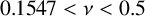Again, Djordjevic and Redekopp [Reference Djordjevic and Redekopp13] showed that for all $kh$ , pure capillary waves are modulationally unstable. Hogan [Reference Hogan17] and Kawahara [Reference Kawahara22] stated that CGWs in deep water are modulationally unstable if $0<\nu <0.1547$ and 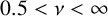$0.5<\nu <\infty $ . Therefore, they remarked that the stability properties of a uniform wave train are critically affected by considering the effect of capillarity.

3 Modulational instability

The simplest solution of (2.14) is given by

$$ \begin{align*} a= a_{0}\,\mathrm{exp}(-i\mu_{1} a_0^{2}\tau), \end{align*} $$

where $ a_0 \in \mathbb {R}$ , and is known as the wave steepness.

To study the modulational instability, we consider the following infinitesimal perturbations:

(3.1) $$ \begin{align} a= a_{0}(1+ a{'})\,e^{~i(\theta{'}-\mu_{1} a_0^{2}\tau)}. \end{align} $$

Substituting (3.1) in the NSE (2.14), linearizing and considering

$$ \begin{align*} \begin{aligned} \begin{pmatrix} a{'}\\ \theta{'} \end{pmatrix} \propto e^{i(pX-\Lambda\tau)}, \end{aligned} \end{align*} $$

we get the nonlinear dispersion relation given by (see [Reference Dhar and Das11])

(3.2) $$ \begin{align} \Lambda=\gamma_{1}p-\gamma_{3}p^{3}- a_0^{2}\mu_{2}p\pm\sqrt{\gamma_{2}p^{2}(\gamma_{2}p^{2}+2 a_0^{2}\mu_{1}-2 a_0^{2}\mu_{4}| p|)}, \end{align} $$

where $\Lambda $ and p are the perturbed frequency and wavenumber, respectively. From (3.2), instability occurs when

(3.3) $$ \begin{align} \gamma_{2}(\gamma_{2}p^{2}+2 a_0^{2}\mu_{1}-2 a_0^{2}\mu_{4}| p|)<0, \end{align} $$

which leads to a complex-valued $\Lambda $ . If this condition is satisfied, the growth rate of the infinitesimal perturbations, expressed as the imaginary part of $\Lambda $ , becomes

(3.4) $$ \begin{align} \Lambda_{i}=p\sqrt{-\gamma_{2}(\gamma_{2}p^{2}+2 a_0^{2}\mu_{1}-2 a_0^{2}\mu_{4}| p|)}, \end{align} $$

where subscript i indicates ‘the imaginary part’.

From (3.3), the instability bandwidth is given by

(3.5) $$ \begin{align} p=\bigg[\sqrt{\frac{-2\mu_1}{\gamma_{2}}} +\frac{\mu_4}{\gamma_{2}} a_0\bigg]a_0. \end{align} $$

The growth rate of instability attains a maximum value $\Lambda _{im}$ given by

(3.6) $$ \begin{align} \Lambda_{im}=|\mu_{1}|\bigg[1-\frac{\mu_{4}}{\mu_{1}}\bigg(-\frac{\mu_{1}}{\gamma_{2}}\bigg)^{1/2} a_{0} \bigg] a_0^{2}. \end{align} $$

It is important to note that without vorticity, instability is possible when

(3.7) $$ \begin{align} (2\nu-1)(3\nu^2+6\nu-1)>0 \end{align} $$

for which the ranges of $\nu $ become

(3.8) $$ \begin{align} 0<\nu<\frac{2}{\sqrt{3}}-1=0.1547 \quad \text{and} \quad 0.5<\nu<\infty. \end{align} $$

These results are in agreement with the results found by Zakharov et al. [Reference Zakharov45]. Here, the lower value $0.1547$ of $\nu $ corresponds to the minimum group velocity and the upper value $0.5$ of $\nu $ to the first Wilton [Reference Wilton43] ripple, where the wave has the same phase velocity as its first harmonic. Lighthill [Reference Lighthill24] showed that the range $0.1547<\nu <0.5$ , where instability is impossible, corresponds to an elliptic dispersion equation. Outside the range, it is hyperbolic.

3.1 Capillary-gravity waves

First, we start with the general case where the restoring forces include both surface tension and gravity. For waves of wavelength $4$ cm, surface tension $T=74$ dyne/cm, gravity acceleration $g=981$ cm/sec $^2$ and density $\rho =1$ gm/cm $^3$ , the value of $\nu $ becomes $0.005$ . Hsu et al. [Reference Hsu, Kharif, Abid and Chen18] have also considered the same value of $\nu $ to study the effect of capillarity and therefore, like Hsu et al. [Reference Hsu, Kharif, Abid and Chen18], we take the value of $\nu =0.005$ in our paper.

The growth rate of instability $\Lambda _i$ given by (3.4) against perturbed wavenumber p for different values of vorticity $\overline {\Omega }$ , surface tension $~\nu $ and the wave steepness $ a_0$ is presented in Figure 2. It is observed that the growth rate $\Lambda _i$ is amplified in the presence of negative vorticity ( $\overline {\Omega }>0$ ) and is diminished in the presence of positive vorticity ( $\overline {\Omega }<0$ ). The effect of surface tension is to reduce slightly the growth rate giving a stabilizing influence, consistent with the results of Dhar and Kirby [Reference Dhar and Kirby12]. Again, the growth rate of instability increases with the increase of $ a_0$ .

Figure 2 Plot of growth rate $\Lambda _i$ against p for different $\overline {\Omega }$ and $\nu $ : (a) $ a_0=0.1$ ; (b) $ a_0=0.2$ .

Figure 3 $\Lambda _{im}$ against $ a_0$ for some values of $\overline {\Omega }$ and $\nu $ ; dash-dotted and dotted lines represent third-order results; dashed and solid lines represent fourth-order results.

Figure 3 shows the effects of $\overline {\Omega }$ and $\nu $ on the maximum growth rate of instability $\Lambda _{im}$ . Here, the key point is that the fourth-order results considerably modify the instability property, namely, the maximum growth rate, as compared with the third-order results, and it turns out that the most notable contribution comes from the wave-induced mean flow which corresponds to the term involving the Hilbert transform in (2.14). It is found that $\Lambda _{im}$ obtained from fourth-order results first increases with the increase of $ a_0$ and then its value diminishes, whereas the growth rate obtained from third-order results increases steadily with $ a_0$ . As shown in this figure, without shear and capillarity, the curve obtained from fourth-order results is the same as the curve found by Dysthe [Reference Dysthe14] in Figure 2 and surprisingly close to the exact results of Longuet-Higgins [Reference Longuet-Higgins25, Reference Longuet-Higgins26] for $ a_{0}<0.3$ . Thus, our results agree fairly well with the results of Longuet-Higgins [Reference Longuet-Higgins25, Reference Longuet-Higgins26].

In Figure 4, we have plotted the modulational instability spectrum $\Lambda _i$ in the $(a_{0},p)$ plane for different values of $\overline {\Omega }$ and $\nu $ . It is shown that the positive vorticity $(\overline {\Omega }<0)$ reduces the instability region, whereas the negative vorticity $(\overline {\Omega }>0)$ has an adverse effect.

Figure 4 Fourth-order instability spectrum $\Lambda _i$ in $( a_0,p)$ plane for different $\overline {\Omega }$ and $\nu $ : (a) $\overline {\Omega }=-0.5,~\nu =0$ ; (b) $\overline {\Omega }=-0.5,~\nu =0.005$ ; (c) $\overline {\Omega }=2,~\nu =0$ ; (d) $\overline {\Omega }=2,~\nu =0.005$ . S and I represent the modulational stability and instability regions, respectively.

3.2 Pure capillary waves

We now deal with the case of pure capillary waves on water of infinite depth, that is, when the restoring force is derived from the surface tension alone. Therefore, for the case of pure capillary waves in the presence of vorticity, we have $\nu \rightarrow \infty $ . The corresponding analytical expressions for $\gamma _{1},~\gamma _{2},~\mu _{1},~\mu _{4}$ as $\nu \rightarrow \infty $ become respectively

$$ \begin{gather*} \tilde{\gamma_{1}}=\frac{3(1+\overline{\Omega})}{2+\overline{\Omega}},\\ \tilde{\gamma_{2}}=\frac{3(1+\overline{\Omega}+\overline{\Omega}^{2})(1+\overline{\Omega})}{(2+\overline{\Omega})^{3}},\\ \tilde{\mu_{1}}=-\frac{(1+\overline{\Omega}^2)(3+11\overline{\Omega}-3\overline{\Omega}^{2})+\overline{\Omega}(3+23\overline{\Omega})}{24(1+\overline{\Omega})(2+3\overline{\Omega})},\\ \tilde{\mu_{4}} =\frac{2+\overline{\Omega}}{4(1-\gamma_{1}\overline{\Omega})}. \end{gather*} $$

We can verify that the expressions for $\tilde {\gamma _{2}}$ and $\tilde {\mu _{1}}$ are identical with those of Hsu et al. [Reference Hsu, Kharif, Abid and Chen18]. In Figure 5, we have plotted the growth rate of instability given by (3.4) for pure capillary waves as a function of p for different values of $\overline {\Omega }$ and $ a_0$ . This figure suggests that $\Lambda _i$ increases for negative vorticity and decreases for positive vorticity, and it also increases as the wave steepness $ a_0$ increases. Moreover, $\Lambda _i$ increases with the increase of wavenumber p up to certain value of p and then decreases. It is important to note that $\Lambda _i$ found from fourth-order results is much higher than that obtained from third-order results when $\overline {\Omega }>0$ . The influence of $\overline {\Omega }$ on $\Lambda _{im}$ for pure capillary waves is shown in Figure 6.

Figure 5 Plot of $\Lambda _{i}$ against p for different $\overline {\Omega }$ for pure capillary waves: (a) $ a_0=0.1$ ; (b) $ a_0=0.2$ . Solid and dashed lines represent fourth-order and third-order results, respectively.

Figure 6 Plot of $\Lambda _{im}$ as a function of $ a_0$ for some values of $\overline {\Omega }$ for pure capillary waves. Solid and dashed lines represent fourth-order and third-order results, respectively.

4 Influence of vorticity and capillarity on the Benjamin–Feir index: application to freak waves

Within the outline of random waves, Janssen [Reference Janssen21] presented the notion of BFI, which is the ratio of mean square slope to the normalized width of the spectrum. According to Alber and Saffman [Reference Alber and Saffman2], if the BFI is greater than $1$ , then the waves are unstable, while if BFI is less than $1$ , then the wave field is stable. Therefore, $\text {BFI}=1$ can be taken as the bifurcation point. For initial wave spectra which depend only on the variance and the bandwidth, it can be shown that for the NSE, the large-time solution is fully characterized by the BFI. For the ZIE, this is not true, but the BFI can be considered to be a useful parameter in the case of narrowband waves. Alber [Reference Alber1] reported that the BFI acts as a key role in the homogeneous theory of wave–wave interactions.

The dimensional form of the NSE (6.1) in a frame of reference propagating with the group velocity can be written as

(4.1) $$ \begin{align} i\frac{\partial a}{\partial \tau}-\frac{\omega_0}{k_0^{2}}\gamma_{2}\frac{\partial^2 a}{\partial X^2}=\omega_{0}k_0^{2}\mu_{1}| a|^{2} a+\omega_0 k_0\mu_{4} a \mathcal{H}\bigg[\frac{\partial}{\partial X}(| a|^{2})\bigg]. \end{align} $$

Like Onorato et al. [Reference Onorato, Osborne, Serio, Cavaleri, Brandini and Stansberg31], we rewrite (4.1) by transforming the variables $\tilde { a}= a/ a_0$ , $\tilde {X}=\Delta k X$ , $\tilde {\tau }=\omega _{0}\gamma _{1}(\Delta k/k_0)^{2}\tau $ as follows:

(4.2) $$ \begin{align} i\frac{\partial a}{\partial \tau}-\frac{\partial^2 a}{\partial X^2}=\bigg(\frac{ a_{0}k_0}{\Delta k/k_0}\bigg)^{2}\bigg(\frac{\mu_1}{\gamma_2}\bigg)| a|^{2} a+\frac{( a_{0}k_0)^{2}}{\Delta k/k_0}\frac{\mu_4}{\gamma_2} a \mathcal{H}\bigg[\frac{\partial}{\partial X}(| a|^{2})\bigg], \end{align} $$

where tildes of the variables $ a,X$ and $\tau $ have been deleted. Here, $\Delta k$ represents a typical spectral width. From the NSE, Onorato et al. [Reference Onorato, Osborne, Serio, Cavaleri, Brandini and Stansberg31] defined the BFI in the context of freak waves in random sea states as the square root of the coefficient of the third-order nonlinear term of (4.2) which is given by

$$ \begin{align*} \mathrm{BFI}=\frac{ a_{0}k_0}{\Delta k/k_0}\sqrt{\frac{\lvert\mu_1\rvert}{\gamma_{2}}}. \end{align*} $$

Figure 7 Plot of BFI due to third-order results as a function of $\overline {\Omega }$ for $\nu =0,~0.005$ .

The influence of water depth on the BFI was studied by Onorato et al. [Reference Onorato, Osborne, Serio, Cavaleri, Brandini and Stansberg31], and they reported that the BFI approaches one with increasing water depth and approaches zero for shallower water. From Figure 7, one can observe that BFI takes the value of 1 for $\overline {\Omega }=0$ , $\nu =0$ , consistent with the results of Onorato et al. [Reference Onorato, Osborne, Serio, Cavaleri, Brandini and Stansberg31]. Later on, Thomas et al. [Reference Thomas, Kharif and Manna40] investigated the influence of water depth h, as h tends to infinity, and also the $\overline {\Omega }$ on the BFI. In this paper, we have shown the importance of the influence of $\overline {\Omega }$ and $\nu $ on the BFI. As shown in Figure 7, for fixed values of $\nu $ and $\boldsymbol {\overline {\Omega }>0}$ , the BFI and hence nonlinearity increase with the increase of $\overline {\Omega }$ , and for $\overline {\Omega }<0$ , the presence of vorticity diminishes the BFI, consistent with the results of Thomas et al. [Reference Thomas, Kharif and Manna40] for $\nu =0$ . So, we may expect that the number of freak waves increases for $\overline {\Omega }>0$ . It seems pertinent to mention that this result was first obtained numerically by Osborne and Onorato. Furthermore, as $\nu $ increases, the BFI first decreases up to a certain value of $\overline {\Omega }$ and then increases. We also observe that the ratio between nonlinearity and dispersion increases with the increase of $\overline {\Omega }>0$ .

5 Effect of shear current on Peregrine breather

The modulational instability of surface waves can well be studied by the NSE, so this equation is generally used to examine the behaviour of freak waves (see [Reference Chabchoub, Akhmediev and Hoffmann5, Reference Onorato, Osborne, Serio and Bertone30, Reference Osborne, Onorato and Serio32]). It has been ascertained that several aspects of the dynamics of freak waves that are shown to appear as a result of nonlinear self-focusing events can be explained by the NSE. From a physical point of view, it is well known that the NSE overestimates the instability region and the maximum wave amplitude with respect to higher-order models. Further, the results obtained from the NSE give important physical insight into the formation of freak waves. These freak waves emerge when the waves are sufficiently steep for nonlinear focusing (modulational instability) to triumph over the spreading of energy by linear dispersion. Hence, the Benjamin–Feir instability occurs. Peregrine [Reference Peregrine34] found an important localized outcome of the NSE in both space and time that is known as the Peregrine breather. Here, we find the Peregrine breather solution that can be taken into account as the prototype of freak waves because its peak amplitude can reach three times the initial value. From (2.14), we can write the third-order NSE

(5.1) $$ \begin{align} i\frac{\partial a}{\partial \tau}-\gamma_{2}\frac{\partial^2 a}{\partial X^2}=\mu_{1}| a|^{2} a. \end{align} $$

Let us write a in the form

(5.2) $$ \begin{align} a=\epsilon[ B e^{{i(k_0 x-\omega_0 t)}}+\text{c.c.}]+O(\epsilon^2), \end{align} $$

and then (5.1) becomes

(5.3) $$ \begin{align} i\frac{\partial B}{\partial \tau}-\gamma_{2}\frac{\partial^2 B}{\partial X^2}-\overline{\mu}_{1}| B |^{2}B=0, \end{align} $$

where $\overline {\mu }_{1}=\{(1+\nu )/(1+\overline {\Omega })\}^{2}\mu _1$ .

A dimensionless form of (5.3) can be found by using the following re-scaled variables:

(5.4) $$ \begin{align} \overline{X}=\sqrt{\frac{-\overline{\mu}_{1}}{2\gamma_2}} a_0 X, \quad \overline{\tau}=-\frac{1}{2}\overline{\mu}_{1} a_0^{2}\tau,\quad \overline{B}=\frac{B}{ a_0}. \end{align} $$

Using (5.4), (5.3) becomes

(5.5) $$ \begin{align} i\frac{\partial \overline{B}}{\partial \overline{\tau}}+\frac{\partial^2 \overline{B}}{\partial \overline{X}^2}+2| \overline{B} |^{2}\overline{B}=0. \end{align} $$

The PB solution of (5.5) is given by

(5.6) $$ \begin{align} \overline{B}(\overline{X},\overline{\tau})=e^{(2i\overline{\tau})}\bigg\{\frac{4(1+4i\overline{\tau})}{1+4\overline{X}^{2}+16\overline{\tau}^{2}}-1\bigg\}. \end{align} $$

This solution is localized in both space and time with focusing corresponding to ${\overline {X}=0,~\overline {\tau }=0}$ and the maximum amplitude for $\overline {X}=0,~\overline {\tau }=0$ is 3.

Using (5.4) in (5.6), the breather solution can be rewritten in the following dimensional form:

$$ \begin{align*} B(X,\tau)= a_{0} e^{{(-i\overline{\mu}_{1} a_0^{2}\tau)}}\bigg\{\frac{4\gamma_{2}(1-2i\overline{\mu}_{1} a_0^{2}\tau)}{\gamma_{2}-2\overline{\mu}_{1} (X^2-2\gamma_{2}\overline{\mu}_{1}\tau^2a_{0}^2)a_{0}^2}-1\bigg\}. \end{align*} $$

Figure 8 The wave envelope against space with different $\overline {\Omega }$ and $\nu $ .

The most important characteristic of the breather solution is that its maximum value can be found at a single point in the space–time domain and this decreases exponentially away from the localized region.

The surface elevation of freak waves is of great significance in practical applications. From (5.2), we find the expression of surface elevation amplitude accurate to first order as follows:

$$ \begin{align*} a(x,t)&=\epsilon a_{0}\bigg[\cos{(k_0 x-\omega_0 t)} \bigg\{\bigg(\frac{4\gamma_{2}}{\zeta}-1 \bigg)\cos{\Theta}-\frac{8\gamma_{2}\Theta}{\zeta}\sin{\Theta} \bigg\} \nonumber \\ & \quad + \sin{(k_0 x-\omega_0 t)} \bigg\{\bigg(\frac{4\gamma_{2}}{\zeta}-1 \bigg)\sin{\Theta}+\frac{8\gamma_{2}\Theta}{\zeta}\cos{\Theta} \bigg\}\bigg], \end{align*} $$

where $\Theta =\overline {\mu }_{1} a_0^{2}t$ and $\zeta =\gamma _{2}(1+4\overline {\mu }_1^2a_{0}^4t^2)-2\overline {\mu }_{1} a_0^{2}(x-\overline {c}_{g}t)^{2}.$

The effect of shear current on the PB solution for different $\overline {\Omega }$ and $\nu $ is shown in Figures 8 and 9. It is found that the positive vorticity $(\overline {\Omega }<0)$ increases the breather span in both space and time, whereas the negative vorticity $(\overline {\Omega }>0)$ has the opposite effect.

Figure 9 The Peregrine breather with $ a_{0}=0.2~m,~\nu =0,~0.005$ and different values of $\overline {\Omega }=-0.4,~0,~0.4$ .

Figure 10 shows the surface elevation amplitude $ a$ as a function of space and time for different $\overline {\Omega }$ and $\nu $ . It is observed that the surface elevation amplitude is reduced by negative vorticity $(\overline {\Omega }>0)$ , whereas it is amplified by positive vorticity $(\overline {\Omega }<0)$ . Furthermore, the effect of $\nu $ is to diminish the amplitude a.

Figure 10 Plot of wave amplitude $ a$ against space and time with $\omega =5\,\mathrm {Hz},~ a_{0}=0.2\,\mathrm {m},~\overline {\Omega }=-0.5,~0,~0.5$ and $\nu =0,0.005$ .