


1 Introduction
The Jansen–Rit model [Reference Jansen and Rit16, Reference Jansen, Zouridakis and Brandt17] is a well-established neural mass model of the activity of a local cortical circuit in the human brain. The model builds on the earlier work of Lopes da Silva et al. [Reference Lopes da Silva, Hoeks, Smits and Zetterberg21, Reference Lopes da Silva, van Rotterdam, Barts, van Heusden and Burr22] and Freeman [Reference Freeman12]. They developed mathematical models to simulate spontaneous brain activity, which can be recorded noninvasively, to investigate the mechanisms behind specific types of electroencephalogram (EEG) field potentials. Their focus was on understanding the origins of alpha-like activity – a rhythmic EEG pattern with a frequency range of 8–12 Hz, most prominent during restful states with closed eyes.
Neuronal activity detected by EEG results from the combined excitatory and inhibitory postsynaptic potentials generated by large groups of neurons, such as cortical columns in the cerebral cortex, firing at the same time. Jansen et al. [Reference Jansen, Zouridakis and Brandt17] and Jansen and Rit [Reference Jansen and Rit16] extended Lopes da Silva’s lumped parameter model [Reference Lopes da Silva, Hoeks, Smits and Zetterberg21, Reference Lopes da Silva, van Rotterdam, Barts, van Heusden and Burr22] by incorporating an excitatory feedback loop from local interneurons in addition to the original populations of inhibitory interneurons and excitatory pyramidal cells to investigate the significance of excitatory connections over long distances. Although the Jansen–Rit model [Reference Jansen and Rit16], as illustrated in Figure 1(a), is a simplification of the complexity of neural connections in cortical regions of the brain, it is able to generate a range of wave forms and rhythms resembling EEG recordings. Accordingly, it has been extensively employed to simulate brain rhythmic activity recorded by EEG (see [Reference David and Friston7, Reference Stefanovski, Triebkorn, Spiegler, Diaz-Cortes, Solodkin, Jirsa, McIntosh and Ritter26] and references therein). The Jansen–Rit model has been extended further by Wendling et al. [Reference Wendling, Bellanger, Bartolomei and Chauvel29] to study epileptic-like oscillations by the addition of a fast inhibitory interneuron population. This model has since gained significant attention in studies of epileptic seizures [Reference Coletti and Slavova5, Reference Wendling, Bellanger, Bartolomei and Chauvel29]. Furthermore, the Jansen–Rit model has been used to simulate event-related potentials (ERPs) by applying pulse-like inputs, allowing for the replication and analysis of EEG responses to external stimuli. Notably, the interaction between cortical columns has been found to play a key role in generating visual evoked potentials (VEPs) [Reference Jansen, Zouridakis and Brandt17].

Figure 1 (a) Interactions among three neuronal populations in a local circuit of a single cortical column in the cerebral cortex of a brain modelled by (2.1): pyramidal cells ( $Y_1$
), and excitatory (
$Y_1$
), and excitatory ( $Y_3$
, EINs) and inhibitory (
$Y_3$
, EINs) and inhibitory ( $Y_2$
, IINs) interneurons. (b) Blue axis shows the sigmoid profile of
$Y_2$
, IINs) interneurons. (b) Blue axis shows the sigmoid profile of ${\mathrm {Sigm}}$
, defined in (2.2), with slope
${\mathrm {Sigm}}$
, defined in (2.2), with slope $r=0.56$
at threshold
$r=0.56$
at threshold $y_0=6$
mV (vertical dotted line), at which half-maximum
$y_0=6$
mV (vertical dotted line), at which half-maximum $e_0$
of
$e_0$
of ${\mathrm {Sigm}}$
is achieved. (b) Black axis shows dimensionless sigmoid
${\mathrm {Sigm}}$
is achieved. (b) Black axis shows dimensionless sigmoid ${\mathrm {S}}$
, given in (3.3), for maximal slope value
${\mathrm {S}}$
, given in (3.3), for maximal slope value $1/(4\epsilon )=0.25/0.024\approx 10.5$
at activation threshold
$1/(4\epsilon )=0.25/0.024\approx 10.5$
at activation threshold $y_{0,1}=0.08$
(nondimensionalized threshold
$y_{0,1}=0.08$
(nondimensionalized threshold $y_{0,1}$
for excitatory populations indicated by black vertical dotted line). See Tables 1 and 2 for other parameters of
$y_{0,1}$
for excitatory populations indicated by black vertical dotted line). See Tables 1 and 2 for other parameters of ${\mathrm {Sigm}}$
and
${\mathrm {Sigm}}$
and ${\mathrm {S}}$
.
${\mathrm {S}}$
.
The rhythms generated by the Jansen–Rit model can be associated with different behaviours, levels of excitability and states of consciousness. Using the parameter settings suggested by Jansen and Rit [Reference Jansen and Rit16], the model produces oscillations around 10 Hz corresponding to alpha-like activity as described by Grimbert and Faugeras [Reference Grimbert and Faugeras13]. Delta rhythms have frequencies between 0.5 and 4 Hz detected during deep stages of nonREM sleep (particularly stages 3 and 4), also known as slow-wave sleep. During these stages, the brain exhibits large-amplitude, low-frequency delta activity. A recent experimental study reports an alpha/delta switch in the prefrontal cortex regulating the shift between positive and negative emotional states [Reference Burgdorf and Moskal4]. Moreover, another very recent study by Brudzynski et al. [Reference Brudzynski, Burgdorf and Moskal3] identifies a transition between positive (associated with alpha rhythms) and negative (associated with delta rhythms) emotions controlled by the arousal system. At the level of neuronal circuits, the alpha rhythm is linked to synaptic long-term potentiation (LTP) in the cortex, while the delta rhythm is associated with synaptic depotentiation (LTD) in the same region. Therefore, understanding what controls the transitions between alpha and delta oscillations in neural circuits enhances our knowledge of how neural circuits regulate brain states and may provide insights into disruptions that affect sleep and cognitive functions.
Grimbert and Faugeras [Reference Grimbert and Faugeras13] analysed the oscillatory behaviour of the Jansen–Rit model using numerical bifurcation analysis. In their work, the external input signal p (see Figure 1(a)) was considered as a bifurcation parameter. The behaviour of the model under variation in p was investigated where all other model parameters were kept fixed and equal to what was originally proposed by Jansen and Rit (see Table 1). They found that the qualitative behaviour of the system changes from steady state to oscillatory behaviour (appearance or disappearance limit cycle) via a Hopf bifurcation. The authors also pointed out that the system displays distinct phenomena such as bistability, limit cycles and chaos. Furthermore, Touboul et al. [Reference Touboul, Wendling, Chauvel and Faugeras27] carried out bifurcation analysis for a nondimensionalized Jansen–Rit model and the extension proposed by Wendling et al. [Reference Wendling, Bellanger, Bartolomei and Chauvel29] in several system parameters, detecting and tracking bifurcations of up to codimension $3$
.
$3$
.
Table 1 Quantities in Jansen–Rit model, (2.1), and their default values and dimensions [Reference Jansen and Rit16].
The transition between alpha and delta oscillations is linked to a notable feature exhibited by the Jansen–Rit neural mass model: a sharp qualitative change in the oscillations’ time profiles and frequencies occurs over a small parameter range without change of stability and no (or little) hysteresis. Hence, the underlying mathematical mechanism cannot be a generic bifurcation as found in textbooks [Reference Guckenheimer and Holmes14, Reference Kuznetsov19]. Recent work by Forrester et al. [Reference Forrester, Crofts, Sotiropoulos, Coombes and O’Dea11], which developed an analysis of a large network of interacting neural populations of Jansen–Rit cortical column models in the absence of noise, identified the alpha–delta transition as a “false bifurcation”. They used an arbitrary geometric feature of the periodic orbit (an inflection point) and associated it with the qualitative changes of the periodic orbits. The feature of the orbits could then be expressed as a zero problem and tracked in the two-parameter space $(A, B)$
, where A and B are the gain (strength) of excitatory and inhibitory responses, respectively. This is similar to the approach proposed by Rodrigues et al. [Reference Rodrigues, Barton, Marten, Kibuuka, Alarcon, Richardson and Terry25], who tracked qualitative changes in orbit shapes in an EEG model of absence seizures (such as Marten et al. [Reference Marten, Rodrigues, Benjamin, Terry and Richardson23]). Study of alpha and delta frequency oscillations based on different parameter settings has been performed by Ahmadizadeh et al. [Reference Ahmadizadeh, Karoly, Nešić, Grayden, Cook, Soudry and Freestone1]. They showed that a model of two coupled cortical columns can produce delta activity as the gain strength between the two cortical columns is varied (see Figure 12T1 of [Reference Ahmadizadeh, Karoly, Nešić, Grayden, Cook, Soudry and Freestone1] for delta-like activity). Their model can also produce alpha-like activity, where the frequency of oscillation lies in the alpha frequency band but the amplitude changes.
$(A, B)$
, where A and B are the gain (strength) of excitatory and inhibitory responses, respectively. This is similar to the approach proposed by Rodrigues et al. [Reference Rodrigues, Barton, Marten, Kibuuka, Alarcon, Richardson and Terry25], who tracked qualitative changes in orbit shapes in an EEG model of absence seizures (such as Marten et al. [Reference Marten, Rodrigues, Benjamin, Terry and Richardson23]). Study of alpha and delta frequency oscillations based on different parameter settings has been performed by Ahmadizadeh et al. [Reference Ahmadizadeh, Karoly, Nešić, Grayden, Cook, Soudry and Freestone1]. They showed that a model of two coupled cortical columns can produce delta activity as the gain strength between the two cortical columns is varied (see Figure 12T1 of [Reference Ahmadizadeh, Karoly, Nešić, Grayden, Cook, Soudry and Freestone1] for delta-like activity). Their model can also produce alpha-like activity, where the frequency of oscillation lies in the alpha frequency band but the amplitude changes.
Our paper starts from the observation that after nondimensionalization (as done by Touboul et al. [Reference Touboul, Wendling, Chauvel and Faugeras27]) the activation function for excitatory inputs has steep slopes and small thresholds. The small threshold models that neurons begin to activate with small input or stimulus, indicating high sensitivity to incoming signals. A steep slope signifies that once the activation begins, it escalates rapidly, with the neurons’ response intensity increasing sharply as input crosses the threshold. Hence, it makes sense to introduce a small parameter $\epsilon $
equal to a quarter of the inverse of the activation slope. The singular limit
$\epsilon $
equal to a quarter of the inverse of the activation slope. The singular limit $\epsilon \to 0$
replaces the activation functions by all-or-nothing switches represented mathematically by Heaviside functions. In this singular limit, we can locate most bifurcations of equilibria with simple formulae. We can also identify the underlying mechanism for the alpha–delta transition. During alpha-type oscillations, the minimum of the potential of the pyramidal cells always stays above the threshold for switching off the excitatory feedback (see Figure 5). At the transition, the minimum then “touches” this threshold. If the potential falls below the threshold even briefly, the excitatory feedback collapses leading to all potentials dropping to zero. This type of “touching of a threshold” is a typical bifurcation in a system with discontinuous switches, called a grazing bifurcation [Reference di Bernardo, Budd, Champneys and Kowalczyk9, Reference Kuznetsov, Rinaldi and Gragnani20]. Our Figure 6 shows how this grazing bifurcation is an accurate approximation of the boundary between alpha- and delta-type oscillations for the value
$\epsilon \to 0$
replaces the activation functions by all-or-nothing switches represented mathematically by Heaviside functions. In this singular limit, we can locate most bifurcations of equilibria with simple formulae. We can also identify the underlying mechanism for the alpha–delta transition. During alpha-type oscillations, the minimum of the potential of the pyramidal cells always stays above the threshold for switching off the excitatory feedback (see Figure 5). At the transition, the minimum then “touches” this threshold. If the potential falls below the threshold even briefly, the excitatory feedback collapses leading to all potentials dropping to zero. This type of “touching of a threshold” is a typical bifurcation in a system with discontinuous switches, called a grazing bifurcation [Reference di Bernardo, Budd, Champneys and Kowalczyk9, Reference Kuznetsov, Rinaldi and Gragnani20]. Our Figure 6 shows how this grazing bifurcation is an accurate approximation of the boundary between alpha- and delta-type oscillations for the value $\epsilon \approx 1/40$
corresponding to the parameters in the original Jansen–Rit model.
$\epsilon \approx 1/40$
corresponding to the parameters in the original Jansen–Rit model.
The paper is organized as follows. We present the Jansen–Rit model in Section 2, together with a first numerical bifurcation analysis in one parameter (feedback strength A between excitatory populations). This analysis shows the two types of oscillation (alpha and delta type) and the sharp transition between them. Section 3 first nondimensionalizes the model, identifies a small parameter $\epsilon $
and different ways to take the singular limit
$\epsilon $
and different ways to take the singular limit $\epsilon \to 0$
. In Section 3.3, we derive explicit expressions for the location of equilibria in the limiting piecewise linear system. In Section 3.5, we derive an algebraic system of equations for the periodic orbits of alpha-type, which are piecewise exponentials and for which, one of the components is constant. Using this algebraic system, we detect and track the grazing bifurcation, resulting in Figure 6. As our singular perturbation analysis is only partial, we discuss open questions in Section 4.
$\epsilon \to 0$
. In Section 3.3, we derive explicit expressions for the location of equilibria in the limiting piecewise linear system. In Section 3.5, we derive an algebraic system of equations for the periodic orbits of alpha-type, which are piecewise exponentials and for which, one of the components is constant. Using this algebraic system, we detect and track the grazing bifurcation, resulting in Figure 6. As our singular perturbation analysis is only partial, we discuss open questions in Section 4.
2 The Jansen–Rit model for a single cortical column
Figure 1(a) shows the structure of the Jansen–Rit model for a single cortical column. The model assumes that the cortical column contains two populations of interneurons, one excitatory and one inhibitory, and a population of excitatory pyramidal cells. The model contains two blocks for each population, a linear dynamic block, modelled as a second-order differential equation with the population’s average postsynaptic potential (PSP) $Y_i$
as its output and an average pulse density of action potentials as its input. In Figure 1(a), these are the blocks with label
$Y_i$
as its output and an average pulse density of action potentials as its input. In Figure 1(a), these are the blocks with label $Y_i$
:
$Y_i$
: $Y_1$
is the PSP of the pyramidal cell population (blue diamond in Figure 1(a);
$Y_1$
is the PSP of the pyramidal cell population (blue diamond in Figure 1(a); $Y_2$
is the PSP of the inhibitory interneuron population (red ellipse in Figure 1(a)); and
$Y_2$
is the PSP of the inhibitory interneuron population (red ellipse in Figure 1(a)); and $Y_3$
is the PSP of the excitatory interneuron population (green ellipse in Figure 1(a)). The other block for each population is a nonlinear sigmoid-type activation function (the blocks labelled “Sigm” in Figure 1(a)) from the PSP into an average pulse density of action potentials.
$Y_3$
is the PSP of the excitatory interneuron population (green ellipse in Figure 1(a)). The other block for each population is a nonlinear sigmoid-type activation function (the blocks labelled “Sigm” in Figure 1(a)) from the PSP into an average pulse density of action potentials.
The arrows in Figure 1(a) show a positive feedback loop between the pyramidal neuron population ( $Y_1$
) and the excitatory interneuron population (
$Y_1$
) and the excitatory interneuron population ( $Y_3$
), where both connections are excitatory; and a negative feedback loop between the pyramidal cells and the inhibitory interneurons (
$Y_3$
), where both connections are excitatory; and a negative feedback loop between the pyramidal cells and the inhibitory interneurons ( $Y_2$
), where the connection back from the inhibitory neurons to the pyramidal cells is inhibitory. The model incorporates an external excitatory input, labelled
$Y_2$
), where the connection back from the inhibitory neurons to the pyramidal cells is inhibitory. The model incorporates an external excitatory input, labelled $p(t)$
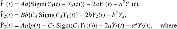
(an average pulse density) representing signalling from other neuronal populations external to the column (Figure 1(a)). The resulting ordinary differential equation (ODE) system corresponding to the schematic diagram in Figure 1(a) is as follows (note that each equation is of order two):
$p(t)$
(an average pulse density) representing signalling from other neuronal populations external to the column (Figure 1(a)). The resulting ordinary differential equation (ODE) system corresponding to the schematic diagram in Figure 1(a) is as follows (note that each equation is of order two):
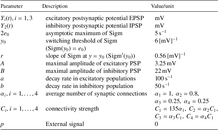
is a nonlinear sigmoid activation function, converting local field postsynaptic potential into firing rate, as shown in Figure 1(b). Its argument y is the average postsynaptic potential in $\text {mV}$
of the neural population. The threshold
$\text {mV}$
of the neural population. The threshold $y_0$
determines the input level at which the firing rate is half of its maximum
$y_0$
determines the input level at which the firing rate is half of its maximum $2{e_0}$
, and r is the slope of
$2{e_0}$
, and r is the slope of ${\mathrm {Sigm}}$
at
${\mathrm {Sigm}}$
at $y_0$
.
$y_0$
.
We restrict our study mostly to the case without external input signal by setting the input $p(t)$
to zero, that is,
$p(t)$
to zero, that is, $p(t)=0$
. In previous studies, the values of
$p(t)=0$
. In previous studies, the values of $p(t)$
have been varied from 120 Hz to 320 Hz as proposed by Jansen and Rit [Reference Jansen and Rit16]. For example, Grimbert and Faugeras [Reference Grimbert and Faugeras13] have performed bifurcation analysis of (2.1) varying the input
$p(t)$
have been varied from 120 Hz to 320 Hz as proposed by Jansen and Rit [Reference Jansen and Rit16]. For example, Grimbert and Faugeras [Reference Grimbert and Faugeras13] have performed bifurcation analysis of (2.1) varying the input $p(t)$
. The quantity
$p(t)$
. The quantity $Y_3(t)-Y_2(t)$
can be related to experiments, because it is proportional to the signals obtained via EEG recordings corresponding to the average local field potential generated by the underlying neuronal populations in the cortical circuits [Reference Jansen, Zouridakis and Brandt17]. In the cortex, pyramidal neurons project their apical dendrites into the superficial layers where the postsynaptic potentials are summed, thereby making up the core of the EEG. The interpretation of all model quantities and their numerical values and dimensions are given in Table 1. The values are set to those proposed by Jansen and Rit [Reference Jansen and Rit16].
$Y_3(t)-Y_2(t)$
can be related to experiments, because it is proportional to the signals obtained via EEG recordings corresponding to the average local field potential generated by the underlying neuronal populations in the cortical circuits [Reference Jansen, Zouridakis and Brandt17]. In the cortex, pyramidal neurons project their apical dendrites into the superficial layers where the postsynaptic potentials are summed, thereby making up the core of the EEG. The interpretation of all model quantities and their numerical values and dimensions are given in Table 1. The values are set to those proposed by Jansen and Rit [Reference Jansen and Rit16].
2.1 Sharp transitions from alpha to delta activity
Figure 2(a) shows the one-parameter bifurcation diagram of the Jansen–Rit model (2.1) for varying excitability scaling factor ${A}$
, which determines maximal amplitude of excitatory postsynaptic potentials (EPSP) of excitatory populations (pyramidal cells
${A}$
, which determines maximal amplitude of excitatory postsynaptic potentials (EPSP) of excitatory populations (pyramidal cells $Y_1$
) and excitatory interneurons (
$Y_1$
) and excitatory interneurons ( $Y_3$
). All other parameters are fixed as listed in Table 1. The y-axis shows the PSP of the excitatory interneurons (
$Y_3$
). All other parameters are fixed as listed in Table 1. The y-axis shows the PSP of the excitatory interneurons ( $Y_3$
). A branch of equilibria (blue) folds back and forth in two saddle node bifurcations (purple squares). Solid curves are stable and dashed curves are unstable parts of the branch. Along the upper part of the branch, the equilibria change stability in three Hopf bifurcations (red diamonds). We focus on the periodic orbits (oscillations) emerging from the Hopf bifurcation at a high value of
$Y_3$
). A branch of equilibria (blue) folds back and forth in two saddle node bifurcations (purple squares). Solid curves are stable and dashed curves are unstable parts of the branch. Along the upper part of the branch, the equilibria change stability in three Hopf bifurcations (red diamonds). We focus on the periodic orbits (oscillations) emerging from the Hopf bifurcation at a high value of ${A}$
(
${A}$
( ${A}\approx 15$
, label (HB)). The black curves show the maximum and minimum values of
${A}\approx 15$
, label (HB)). The black curves show the maximum and minimum values of $Y_3$
along this branch of mostly stable periodic orbits that emanate from this Hopf bifurcation and terminate at the low-
$Y_3$
along this branch of mostly stable periodic orbits that emanate from this Hopf bifurcation and terminate at the low- ${A}$
end in a homoclinic bifurcation of saddle-node on invariant circle type (SNIC; [Reference Izhikevich15]), at which the frequency of oscillation goes to zero as
${A}$
end in a homoclinic bifurcation of saddle-node on invariant circle type (SNIC; [Reference Izhikevich15]), at which the frequency of oscillation goes to zero as ${A}$
approaches the value for the saddle node bifurcation on the lower branch of equilibrium points (
${A}$
approaches the value for the saddle node bifurcation on the lower branch of equilibrium points ( ${A}\approx 7$
).
${A}\approx 7$
).
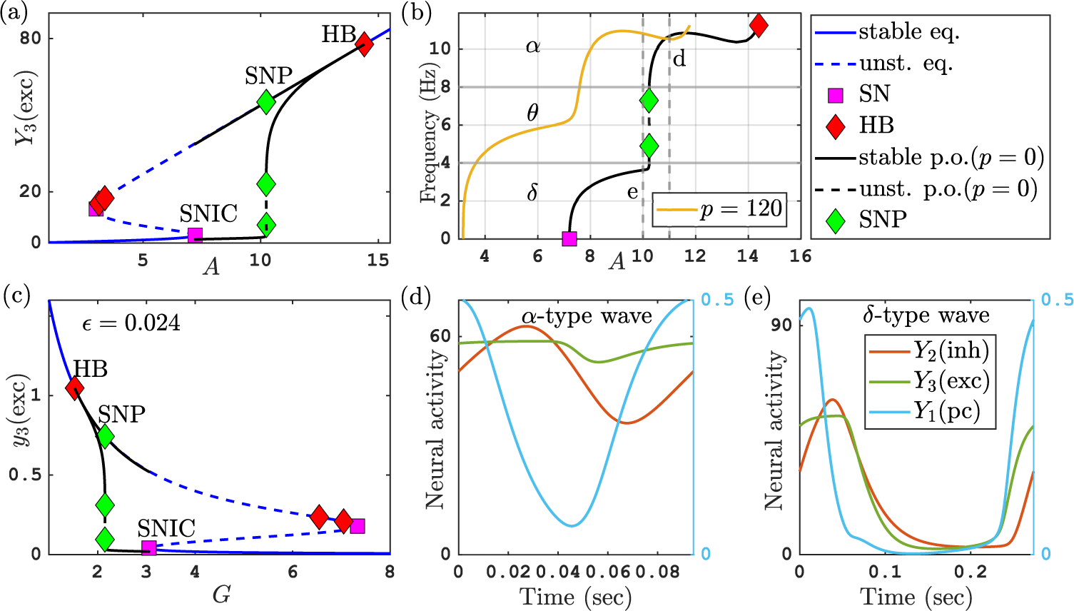
Figure 2 (a) Bifurcation diagram of the Jansen–Rit model (2.1) for varying ${A}$
. (b) Frequency of oscillations with input
${A}$
. (b) Frequency of oscillations with input ${p=0}$
(black) and input
${p=0}$
(black) and input ${p=120}$
(yellow) for varying
${p=120}$
(yellow) for varying ${A}$
, indicating alpha, theta and delta frequency ranges. (c) Same bifurcation diagram as panel (a) but using nondimensionalized quantities
${A}$
, indicating alpha, theta and delta frequency ranges. (c) Same bifurcation diagram as panel (a) but using nondimensionalized quantities $G=B/A$
and
$G=B/A$
and $y_3$
. (d),(e) Time profiles of oscillations in alpha (
$y_3$
. (d),(e) Time profiles of oscillations in alpha ( ${A=11}$
) and delta (
${A=11}$
) and delta ( ${A=10}$
) rhythm regimes corresponding to vertical dashed lines in panel (b). See Tables 1 and 2 for parameters. Computation performed with coco [Reference Dankowicz and Schilder6].
${A=10}$
) rhythm regimes corresponding to vertical dashed lines in panel (b). See Tables 1 and 2 for parameters. Computation performed with coco [Reference Dankowicz and Schilder6].
Figure 2(b) shows the frequency of these oscillations over the range of parameters A where they exist ( ${A}\in [7,14.4]$
). We observe a sharp transition between high-frequency oscillations for A in the range
${A}\in [7,14.4]$
). We observe a sharp transition between high-frequency oscillations for A in the range $[10.2,14.4]$
, where the frequency (in Hz) is in the range
$[10.2,14.4]$
, where the frequency (in Hz) is in the range $[8,11]$
, and low-frequency oscillation for
$[8,11]$
, and low-frequency oscillation for ${A}$
in the range
${A}$
in the range $[7,10.2]$
, where the frequency is approximately
$[7,10.2]$
, where the frequency is approximately $4$
Hz and below. The oscillation frequencies on either side of the transition are associated with wakefulness state (alpha-like activity, around
$4$
Hz and below. The oscillation frequencies on either side of the transition are associated with wakefulness state (alpha-like activity, around $10$
Hz) and deep sleep (delta-like activity, around
$10$
Hz) and deep sleep (delta-like activity, around $2$
Hz).
$2$
Hz).
Figures 2(d) and 2(e) show that this change in frequency is accompanied with a qualitative change in the time profiles of the orbits. The alpha-type fast oscillations have a four-phase profile typical for an oscillatory negative feedback loop (compare Figure 2(d) and note that the scale differs between different outputs such that Figure 2(d) has two y-axes):
-
• ( $0$
–
$0.02$
s) high pyramidal cell output (
$Y_1$
, blue) causes rising inhibition (
$Y_2$
, red);
$0$
–
$0.02$
s) high pyramidal cell output (
$Y_1$
, blue) causes rising inhibition (
$Y_2$
, red); -
• (
$0.02$
–
$0.05$
s) high inhibition causes decrease in pyramidal cell output; -
• (
$0.03$
–
$0.07$
s) low pyramidal cell output causes decreasing inhibition; -
• (
$0.06$
–
$0.1$
s) low inhibition causes rising pyramidal cell output.


Throughout the entire period of the alpha-type oscillation, the pyramidal cell output is supported by a near-constant input from the excitatory interneurons ( $Y_3$
, green). The delta-type (slow) oscillations are shown in Figure 2(e). They show a relaxation-type time profile: pyramidal cell output
$Y_3$
, green). The delta-type (slow) oscillations are shown in Figure 2(e). They show a relaxation-type time profile: pyramidal cell output $Y_1$
(blue) and excitatory interneuron output
$Y_1$
(blue) and excitatory interneuron output $Y_3$
(green) collapse to zero and stay there for some period. This period is determined by how long it takes for inhibition (
$Y_3$
(green) collapse to zero and stay there for some period. This period is determined by how long it takes for inhibition ( $Y_2$
, red) to reach sufficiently low levels to permit pyramidal cell output
$Y_2$
, red) to reach sufficiently low levels to permit pyramidal cell output $Y_1$
and excitatory interneuron output
$Y_1$
and excitatory interneuron output $Y_3$
to rise again. The two time profiles in Figures 2(d) and 2(e) occur for parameter values of A just above (Figure 2(d),
$Y_3$
to rise again. The two time profiles in Figures 2(d) and 2(e) occur for parameter values of A just above (Figure 2(d), $A=11$
) and below (Figure 2(e),
$A=11$
) and below (Figure 2(e), $A=10$
) the transition. The bifurcation diagram shows even a tiny region of bistability, bounded by two saddle-node-of-limit-cycle bifurcations. However, this bistability and the saddle nodes are not a consistent feature for this transition. Figure 2(b) shows a bifurcation diagram for nonzero external input (
$A=10$
) the transition. The bifurcation diagram shows even a tiny region of bistability, bounded by two saddle-node-of-limit-cycle bifurcations. However, this bistability and the saddle nodes are not a consistent feature for this transition. Figure 2(b) shows a bifurcation diagram for nonzero external input ( $p=120$
Hz, yellow curve), where the transition still occurs and is still sharp, occurring in a small parameter region, but without bistability or saddle nodes of limit cycles.
$p=120$
Hz, yellow curve), where the transition still occurs and is still sharp, occurring in a small parameter region, but without bistability or saddle nodes of limit cycles.
Forrester et al. [Reference Forrester, Crofts, Sotiropoulos, Coombes and O’Dea11] detected this transition in their investigation of the Jansen–Rit model (2.1). They demonstrated that it is an essential ingredient in the occurrence of large-scale oscillations in a network of neural populations (which would be measurable by EEG). As the transition is not associated with a bifurcation in parts of the parameter space (see Figure 3 of [Reference Forrester, Crofts, Sotiropoulos, Coombes and O’Dea11]), the authors labelled the transition a “false bifurcation” and tracked it in parameter space by associating it with a feature of the time profile, namely the occurrence of an inflection point. Forrester et al. [Reference Forrester, Crofts, Sotiropoulos, Coombes and O’Dea11] pointed out that “false bifurcations” are usually originating from singular perturbation effects in the system, referring to Desroches et al. [Reference Desroches, Krupa and Rodrigues8] and Rodrigues et al. [Reference Rodrigues, Barton, Marten, Kibuuka, Alarcon, Richardson and Terry25].
To investigate this phenomenon further, we nondimensionalize the Jansen–Rit model (2.1) and identify a small parameter $\epsilon $
for which we can then study the singular limit for the transition from alpha to delta activity. The bifurcation diagram in Figure 2(a) shows a sharp change in the time profile of
$\epsilon $
for which we can then study the singular limit for the transition from alpha to delta activity. The bifurcation diagram in Figure 2(a) shows a sharp change in the time profile of $Y_3$
from nearly constant for alpha activity to an oscillation with excursions close to zero: observe the drop in the minimum of the periodic orbit (black curve) for A slightly above
$Y_3$
from nearly constant for alpha activity to an oscillation with excursions close to zero: observe the drop in the minimum of the periodic orbit (black curve) for A slightly above $10$
.
$10$
.
The numerical bifurcation analysis of the Jansen–Rit model is carried out using the coco toolbox [Reference Dankowicz and Schilder6], which is a matlab-based platform for parameter continuation allowing for bifurcation analysis of equilibria and periodic orbits. Numerical continuation in coco [Reference Dankowicz and Schilder6] and xppaut [Reference Ermentrout10] is used to track stability of equilibria and periodic orbits, and to detect their bifurcations. For numerical integration (simulation), we use xppaut and ode45 (a Runge–Kutta method) in matlab. In all single-parameter bifurcation diagrams, solid curves indicate stable states, while dashed lines are unstable states. Black curves indicate maximum and minimum values of periodic solutions in all bifurcation diagramsFootnote 1.
3 Singular perturbation analysis of Jansen–Rit model
We introduce small parameter $\epsilon>0$
for which, in the limit
$\epsilon>0$
for which, in the limit $\epsilon \to 0$
, the right-hand side (vector field) of system (2.1) becomes a piecewise linear nonsmooth system. First, we nondimensionalize the Jansen–Rit model (2.1) to identify the small parameter.
$\epsilon \to 0$
, the right-hand side (vector field) of system (2.1) becomes a piecewise linear nonsmooth system. First, we nondimensionalize the Jansen–Rit model (2.1) to identify the small parameter.
3.1 Nondimensionalization of the Jansen–Rit model
Touboul et al. [Reference Touboul, Wendling, Chauvel and Faugeras27] present a nondimensionalized version of the Jansen–Rit model. We choose the following dimensionless scale, as proposed by Touboul et al. [Reference Touboul, Wendling, Chauvel and Faugeras27].
-
• Dimensionless time is set according to the internal decay time scale of the excitatory populations,
$t_{\mathrm {new}}=at_{\mathrm {old}}$
, where
${a}$
is given in Table 1. -
• We introduce the decay rate ratio
${b^*}$
of inhibitory to excitatory populations and the ratio G of postsynaptic amplitudes of inhibitory to excitatory populations:
$$ \begin{align*} {b^*}=\frac{{b}}{{a}}, \quad G=\frac{{B}}{{A}}. \end{align*} $$
-
• We rescale the state variables
$Y_1$
,
$Y_2$
,
$Y_3$
such that they are all of order
$1$
at their maximum, introducing a small parameter, (3.1)
$$ \begin{align}\begin{aligned} &\epsilon= \frac{2{a}}{{Br C(2e_0)}} \approx0.024,\\ &y_1(t_{\mathrm{new}})=rC\epsilon Y_1\bigg(\frac{t_{\mathrm{new}}}{a}\bigg),\quad y_i(t_{\mathrm{new}})= r\epsilon Y_i\bigg(\frac{t_{\mathrm{new}}}{a}\bigg)\quad \text{for }i=2,3.\end{aligned} \end{align} $$


We note that in Figures 2(d) and 2(e), the quantities $Y_1$
and
$Y_1$
and $Y_2$
,
$Y_2$
, $Y_3$
are on different y-axes, because they have different orders of magnitude. The nondimensionalization (3.1) ensures that pyramidal cell output
$Y_3$
are on different y-axes, because they have different orders of magnitude. The nondimensionalization (3.1) ensures that pyramidal cell output $y_1$
has the same (order-
$y_1$
has the same (order- $1$
) magnitude as the inhibitory interneurons (
$1$
) magnitude as the inhibitory interneurons ( $y_2$
) and the excitatory interneurons (
$y_2$
) and the excitatory interneurons ( $y_3$
). The quantity
$y_3$
). The quantity $b^*$
is a measure of the difference in internal time scales between inhibitory and excitatory populations. Usually,
$b^*$
is a measure of the difference in internal time scales between inhibitory and excitatory populations. Usually, $b^*<1$
as inhibition is slower. The quantity G is a measure for how strong internal feedback strength from inhibitory populations is compared with excitatory populations.
$b^*<1$
as inhibition is slower. The quantity G is a measure for how strong internal feedback strength from inhibitory populations is compared with excitatory populations.
By substituting these dimensionless dependent variables into (2.1) and applying the chain rule with respect to the dimensionless time scale $t_{\mathrm {new}}$
, we obtain the dimensionless form (using
$t_{\mathrm {new}}$
, we obtain the dimensionless form (using ![]() and
and ![]() also for the new time)
also for the new time)
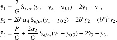
where the new dimensionless sigmoidal transformation is (see Figure 1(b))
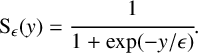 $$ \begin{align} {\operatorname{\mathrm{S}}_{\epsilon} (y)}=\cfrac{1}{1+\exp (-y/\epsilon)}. \end{align} $$
As we have rescaled the PSP’s $Y_i(t)$
, the thresholds in the activation function
$Y_i(t)$
, the thresholds in the activation function ${\mathrm {S}}$
are now different for each neuron population, such that we call them
${\mathrm {S}}$
are now different for each neuron population, such that we call them $y_{0,i}$
. These thresholds
$y_{0,i}$
. These thresholds $y_{0,i}$
, at which the activation
$y_{0,i}$
, at which the activation ${\mathrm {S}}_{\epsilon /a_i}(y-y_{0,i})$
equals
${\mathrm {S}}_{\epsilon /a_i}(y-y_{0,i})$
equals $1/2$
, now show up in (3.2). The new nondimensional activation thresholds are
$1/2$
, now show up in (3.2). The new nondimensional activation thresholds are
 $$ \begin{align} y_{0,1}&=\frac{ry_0}{a_1}\epsilon,& y_{0,2}&=\frac{ry_0}{a_2}\epsilon,& y_{0,3}&=\frac{ry_0}{a_3}\epsilon, \quad \text{where }a_1=a_3=1, a_2=1/4, \end{align} $$
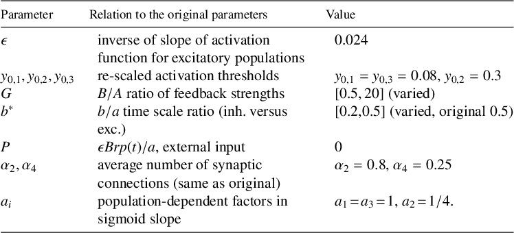
using the parameters from Table 1, which result in the nondimensional parameters shown in Table 2. Note that the main difference to Touboul’s nondimensionalization [Reference Touboul, Wendling, Chauvel and Faugeras27] is that the definition of the sigmoid function includes the scaling factor $\epsilon $
. Figure 2(c) shows the same bifurcation diagram as shown in Figure 2(a), but uses the nondimensionalized quantities G and
$\epsilon $
. Figure 2(c) shows the same bifurcation diagram as shown in Figure 2(a), but uses the nondimensionalized quantities G and $y_3$
. The new primary bifurcation parameter G (the ratio of feedback strengths between inhibition and excitation) is proportional to the inverse of the excitation feedback strength A, such that now, the alpha-to-delta frequency transition occurs for increasing G at
$y_3$
. The new primary bifurcation parameter G (the ratio of feedback strengths between inhibition and excitation) is proportional to the inverse of the excitation feedback strength A, such that now, the alpha-to-delta frequency transition occurs for increasing G at $G\approx 2.2$
. The Hopf bifurcation occurs for low
$G\approx 2.2$
. The Hopf bifurcation occurs for low $G\approx 1.5$
and the SNIC connecting orbit occurs at
$G\approx 1.5$
and the SNIC connecting orbit occurs at $G\approx 3$
.
$G\approx 3$
.
Table 2 Parameter values of the dimensionless model equation (3.2).
3.2 Discussion of smallness of system parameters
In the nondimensionalized model (3.3), the small parameter $\epsilon $
, which equals
$\epsilon $
, which equals $0.024$
, appears in the inverse of the slope of the dimensionless sigmoid
$0.024$
, appears in the inverse of the slope of the dimensionless sigmoid ${\mathrm {S}}_\epsilon $
at
${\mathrm {S}}_\epsilon $
at $y=0$
letting the sigmoid
$y=0$
letting the sigmoid ${\mathrm {S}}_\epsilon $
approach a discontinuous switch in the limit for small
${\mathrm {S}}_\epsilon $
approach a discontinuous switch in the limit for small $\epsilon $
and
$\epsilon $
and $i=1,2,3$
:
$i=1,2,3$
:
 $$ \begin{align} \lim_{\epsilon \to 0} \operatorname{\mathrm{S}}_{\epsilon} (y-y_{0,i}) &= \begin{cases} 0 & \text{if }y<y_{0,i} , \\ 1 & \text{if }y>y_{0,i}. \end{cases} \end{align} $$
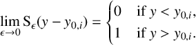
In addition, the activation thresholds $y_{0,i}$
inherit a factor
$y_{0,i}$
inherit a factor $\epsilon $
in (3.4). However, we observe that there are nontrivial factors in front of
$\epsilon $
in (3.4). However, we observe that there are nontrivial factors in front of $\epsilon $
in several places. Since the
$\epsilon $
in several places. Since the $\epsilon $
in the original parameters setting is approximately
$\epsilon $
in the original parameters setting is approximately $1/40$
(so not that small), these factors will influence our strategies for taking the singular limit
$1/40$
(so not that small), these factors will influence our strategies for taking the singular limit $\epsilon \to 0$
.
$\epsilon \to 0$
.
-
• The slope in the activation for the inhibitory interneurons,
$S_{\epsilon /a_2}$
, is
$a_2/(4\epsilon )=1/(16\epsilon )\approx 2.6$
. So, it is further away from the limiting discontinuous switch than the activation of the excitatory populations. -
• The different factors
$ry_0/a_1$
,
$ry_0/a_3$
and
$ry_0/a_2$
of
$\epsilon $
in (3.4) are obtained by substituting the baseline values of the original parameters from Table 1 into system (3.2). We observe that the activation thresholds of excitation are small (
$y_{0,1}=y_{0,3}\approx 0.08$
), but the threshold of inhibition
$y_{0,2}$
(
$y_{0,2}\approx 0.3$
) is not a small quantity.


The smallness of $\epsilon $
expresses that the internal dynamics of neurons in the excitatory populations is fast, leading to small thresholds and steep activation functions after nondimensionalization. The inhibitory neural population is comparatively slower, leading at the population level to a shallower slope of the activation curve and a larger activation threshold [Reference Wilson and Cowan30]. The above observations suggest several possible singular limits.
$\epsilon $
expresses that the internal dynamics of neurons in the excitatory populations is fast, leading to small thresholds and steep activation functions after nondimensionalization. The inhibitory neural population is comparatively slower, leading at the population level to a shallower slope of the activation curve and a larger activation threshold [Reference Wilson and Cowan30]. The above observations suggest several possible singular limits.
-
(a) We let
$\epsilon $
go to zero in the denominator appearing in
${\mathrm {S}}_{\epsilon /a_i}$
for all neuron populations (
$i=1,2,3$
) simultaneously. At the same time, we keep the activation thresholds
$y_{0,i}$
fixed for all populations. This leaves the parameters
$y_{0,i}$
in the model as independent parameters and uses the concrete values from Table 2. -
(b) We let
$\epsilon $
go to zero in the denominator appearing in
${\mathrm {S}}_{\epsilon /a_i}$
for all neuron populations (
$i=1,2,3$
) simultaneously, and we let the activation thresholds
$y_{0,1}$
and
$y_{0,3}$
for the excitatory neuron populations go to zero (either proportional to
$\epsilon $
or at some lower rate). -
(c) We let
$\epsilon $
go to zero for the excitatory neurons populations (
$i=1,3$
) in the slope of the activations
${\mathrm {S}}_{\epsilon /a_i}$
, but keep the activation for the inhibition with a fixed finite slope, equal to
$\approx 10$
(as well as keeping the activation threshold
$y_{0,2}\approx 0.3$
fixed).


We will focus in our analysis on strategy (a) in this paper, because it permits explicit expressions for most equilibria and their bifurcations, and it is sufficient to derive in an implicit algebraic condition for the alpha-to-delta transition. In both limits, the collapse of the alpha-frequency oscillations is a grazing bifurcation [Reference di Bernardo, Budd, Champneys and Kowalczyk9] of periodic orbits in a piecewise linear ODE. In limit (a), the collapse leads to a low excitation equilibrium ( $y_i\ll 1$
for
$y_i\ll 1$
for $i=1,2,3$
), in limit (b), it leads to delta activity.
$i=1,2,3$
), in limit (b), it leads to delta activity.
In the numerical bifurcation diagram in Figure 2(c), the three boundaries for alpha and delta activity are the Hopf bifurcation (onset of alpha frequency oscillations) at $G\approx 1.5$
, the transition between alpha and delta activity at
$G\approx 1.5$
, the transition between alpha and delta activity at $G\approx 2.2$
, and the connecting orbit to a saddle-node (SNIC bifurcation) at
$G\approx 2.2$
, and the connecting orbit to a saddle-node (SNIC bifurcation) at $G\approx 3$
. Two of the boundaries can be found by analysis of equilibria, namely the Hopf bifurcation and the saddle-node bifurcation for small
$G\approx 3$
. Two of the boundaries can be found by analysis of equilibria, namely the Hopf bifurcation and the saddle-node bifurcation for small $y_1$
.
$y_1$
.
For our analysis, the dimensionless external input p is fixed to zero. We use the dimensionless parameter G (the ratio between feedback strength of inhibition versus excitation) as our primary bifurcation parameter. We will later vary $b^*$
, the ratio between internal time scales between inhibition and excitation as a secondary bifurcation parameter.
$b^*$
, the ratio between internal time scales between inhibition and excitation as a secondary bifurcation parameter.
3.3 Equilibrium analysis in the small-
$\epsilon $
limit

Inserting $\epsilon =0$
(or
$\epsilon =0$
(or $\epsilon \ll 1$
) into the activation functions in (3.2) and (3.3) results in an easy-to-interpret limit for equilibria. Setting all derivatives in (3.2) to zero, we obtain that the equilibrium values for
$\epsilon \ll 1$
) into the activation functions in (3.2) and (3.3) results in an easy-to-interpret limit for equilibria. Setting all derivatives in (3.2) to zero, we obtain that the equilibrium values for $y_1$
,
$y_1$
, $y_2$
,
$y_2$
, $y_3$
satisfy the algebraic equations
$y_3$
satisfy the algebraic equations
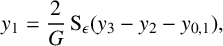 $$ \begin{align} y_1&=\frac{2}{G}\operatorname{\mathrm{S}}_\epsilon(y_3-y_2- y_{0,1}),\end{align} $$
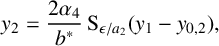 $$ \begin{align} y_2&=\frac{2\alpha_4} {b^*}\operatorname{\mathrm{S}}_{\epsilon/a_2}(y_1-y_{0,2}), \end{align} $$
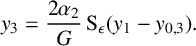 $$ \begin{align} y_3&=\frac{2\alpha_2}{G}\operatorname{\mathrm{S}}_\epsilon(y_1-y_{0,3}). \end{align} $$
The right-hand sides of (3.7) and (3.8) define the equilibrium values $y_2$
and
$y_2$
and $y_3$
as a function of
$y_3$
as a function of $y_1$
. This is also true in the limit
$y_1$
. This is also true in the limit $\epsilon =0$
, whenever
$\epsilon =0$
, whenever $y_1$
is not on the activation threshold (
$y_1$
is not on the activation threshold ( $y_{0,2}$
and
$y_{0,2}$
and $y_{0,3}$
, respectively).
$y_{0,3}$
, respectively).
Inserting (3.7) and (3.8) into (3.6), and taking the Heaviside limit $S_0$
in (3.5) for the activation functions
$S_0$
in (3.5) for the activation functions $S_{\epsilon /a_i}$
(indicating the dependence of
$S_{\epsilon /a_i}$
(indicating the dependence of $y_2$
and
$y_2$
and $y_3$
on
$y_3$
on $y_1$
), leads to the relation
$y_1$
), leads to the relation
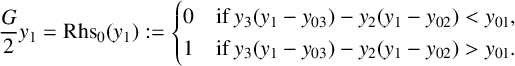 $$ \begin{align} \frac{G}{2}y_1 =\operatorname{\mathrm{Rhs}}_0(y_1):= \begin{cases} 0 & \text{if }y_3(y_1-y_{03})-y_2(y_1-y_{02})< y_{01}, \\ 1& \text{if } y_3(y_1-y_{03})-y_2(y_1-y_{02})> y_{01}. \end{cases} \end{align} $$
Analysis of (3.6)–(3.8) in the limit $\epsilon \to 0$
is supported by Figure 3. Each panel shows the left-hand side of (3.9) (in red) and the right-hand side
$\epsilon \to 0$
is supported by Figure 3. Each panel shows the left-hand side of (3.9) (in red) and the right-hand side ${\mathrm {Rhs}}_0(y_1)$
of (3.9) (in blue) as a function of
${\mathrm {Rhs}}_0(y_1)$
of (3.9) (in blue) as a function of $y_1$
for different values of G, otherwise using the parameter values in Table 2. The (red) left-side function is the straight line
$y_1$
for different values of G, otherwise using the parameter values in Table 2. The (red) left-side function is the straight line $y_1\mapsto Gy_1/2$
. The right-side function
$y_1\mapsto Gy_1/2$
. The right-side function ${\mathrm {Rhs}}_0(y_1)$
is piecewise constant. Defining two critical values for parameter G as
${\mathrm {Rhs}}_0(y_1)$
is piecewise constant. Defining two critical values for parameter G as
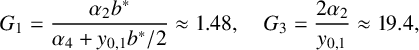 $$ \begin{align} G_1=\frac{\alpha_2b^*}{\alpha_4+y_{0,1}b^*/2}\approx1.48,\quad G_3=\frac{2\alpha_2}{y_{0,1}}\approx19.4, \end{align} $$
(thus, $0<G_1<G_3$
) the right-hand side equals (recall that
$0<G_1<G_3$
) the right-hand side equals (recall that $0<y_{0,3}<y_{0,2}$
)
$0<y_{0,3}<y_{0,2}$
)
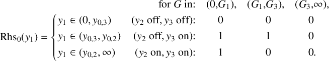 $$ \begin{align*} \begin{aligned} \\ \operatorname{\mathrm{Rhs}}_0(y_1)&= \begin{cases} \\ \\ \ \end{cases} \end{aligned}\hspace{-2em} \begin{aligned} &&\text{for }G\text{ in:}&&(0,&G_1),& (G_1,&G_3),&(G_3,&\infty),\\ y_1&\in(0,y_{0,3})& \text{(}y_2\text{ off}, y_3\text{ off):}&& &0 &&0 &0\\ y_1&\in(y_{0,3},y_{0,2})& \text{(}y_2\text{ off}, y_3\text{ on):} && &1 &&1 &0\\ y_1&\in(y_{0,2},\infty)& \text{(}y_2\text{ on}, y_3\text{ on):} && &1 &&0 & 0 &.\\ \end{aligned} \end{align*} $$
Each intersection of the two lines in Figure 3 is a stable equilibrium if ${\mathrm {Rhs}}_0$
(blue line) is horizontal in the intersection, or an unstable, so-called pseudo-equilibrium [Reference di Bernardo, Budd, Champneys and Kowalczyk9, Reference Kuznetsov, Rinaldi and Gragnani20], if
${\mathrm {Rhs}}_0$
(blue line) is horizontal in the intersection, or an unstable, so-called pseudo-equilibrium [Reference di Bernardo, Budd, Champneys and Kowalczyk9, Reference Kuznetsov, Rinaldi and Gragnani20], if ${\mathrm {Rhs}}_0$
is vertical in the intersection. For
${\mathrm {Rhs}}_0$
is vertical in the intersection. For $\epsilon \ll 1$
but nonzero, the pseudo-equilibria of the piecewise linear limit system will become unstable equilibria with strongly unstable eigenspaces. Table 3 lists the locations of equilibria for all ranges of parameter G, with two additional critical values for G,
$\epsilon \ll 1$
but nonzero, the pseudo-equilibria of the piecewise linear limit system will become unstable equilibria with strongly unstable eigenspaces. Table 3 lists the locations of equilibria for all ranges of parameter G, with two additional critical values for G,
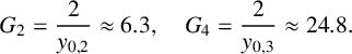 $$ \begin{align} G_2=\frac{2}{y_{0,2}}\approx6.3, \quad G_4=\frac{2}{y_{0,3}}\approx24.8. \end{align} $$
Figure 3(h) shows the resulting bifurcation diagram in the limit of small $\epsilon $
.
$\epsilon $
.
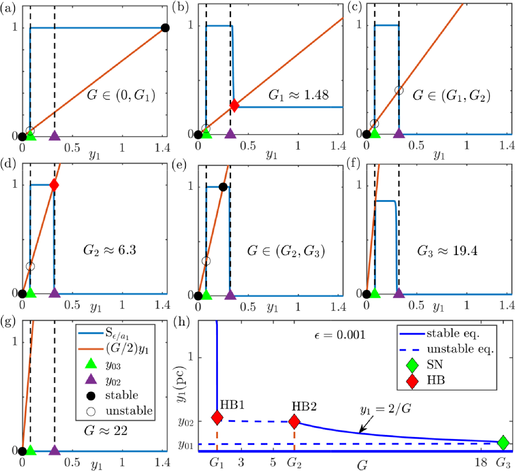
Figure 3 (a)–(g) Intersections between left-hand (red) and right-hand (blue) sides of (3.9) for different bifurcation parameters G (plots used $\epsilon =0.001$
,
$\epsilon =0.001$
, $y_{0,1},y_{0,3}=0.08$
and
$y_{0,1},y_{0,3}=0.08$
and $y_{0,2}=0.3$
). (h) Numerical bifurcation diagram of equilibria in
$y_{0,2}=0.3$
). (h) Numerical bifurcation diagram of equilibria in $(G,y_1)$
-plane obtained by coco [Reference Dankowicz and Schilder6].
$(G,y_1)$
-plane obtained by coco [Reference Dankowicz and Schilder6]. ${\mathrm {S}}_\epsilon /a_1={\mathrm {S}}_\epsilon (y_3-y_2- y_{0,1})$
for
${\mathrm {S}}_\epsilon /a_1={\mathrm {S}}_\epsilon (y_3-y_2- y_{0,1})$
for $y_1$
in (3.6). For other parameters, see Table 2.
$y_1$
in (3.6). For other parameters, see Table 2.
Table 3 Equilibrium points present in system (3.2) for all parameter ranges of G: for critical values of G, see (3.10), (3.11). The index is the number of unstable eigenvalues of the Jacobian in the equilibrium for nonzero $\epsilon $
.
$\epsilon $
.
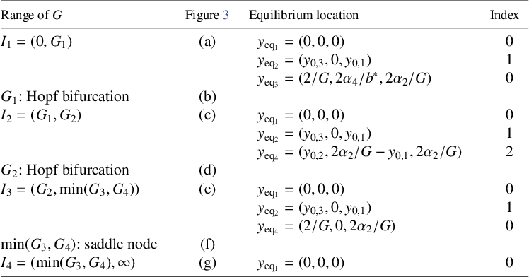
Figure 3(a) shows that for $G<G_1$
, we have a pair of stable and unstable equilibria, both with small values of
$G<G_1$
, we have a pair of stable and unstable equilibria, both with small values of $y_1$
: the unstable equilibrium is a saddle with
$y_1$
: the unstable equilibrium is a saddle with $y_1=y_{0,3}=0.08$
for
$y_1=y_{0,3}=0.08$
for $0<\epsilon \ll 1$
, and the stable equilibrium is a node with a
$0<\epsilon \ll 1$
, and the stable equilibrium is a node with a $y_1$
-value very close to zero, of the order
$y_1$
-value very close to zero, of the order $\exp (-y_{0,1}/\epsilon )$
.
$\exp (-y_{0,1}/\epsilon )$
.
There exists another stable equilibrium, for which $y_1$
is large, equal to
$y_1$
is large, equal to $2/G$
. At
$2/G$
. At $G=G_1$
(Figure 3(b), see (3.10) for value of
$G=G_1$
(Figure 3(b), see (3.10) for value of $G_1$
),
$G_1$
), ${\mathrm {Rhs}}_0$
drops to zero for
${\mathrm {Rhs}}_0$
drops to zero for $y>y_{0,2}$
, which results in a sudden drop of the
$y>y_{0,2}$
, which results in a sudden drop of the $y_1$
-component of the large-
$y_1$
-component of the large- $y_1$
equilibrium to
$y_1$
equilibrium to $y_{0,2}$
and its loss of stability. For positive
$y_{0,2}$
and its loss of stability. For positive $\epsilon $
, this loss of stability is a Hopf bifurcation (see the labelled point HB1 in Figure 3(h)). Figure 3(c) shows the equilibria for
$\epsilon $
, this loss of stability is a Hopf bifurcation (see the labelled point HB1 in Figure 3(h)). Figure 3(c) shows the equilibria for $G\in (G_1,G_2)$
. Figure 3(d) shows the situation at the next critical value of G, the Hopf bifurcation
$G\in (G_1,G_2)$
. Figure 3(d) shows the situation at the next critical value of G, the Hopf bifurcation $G=G_2=2/y_{0,2}$
, when the left-hand side function (red line) goes through the “corner” of
$G=G_2=2/y_{0,2}$
, when the left-hand side function (red line) goes through the “corner” of ${\mathrm {Rhs}}_0$
at
${\mathrm {Rhs}}_0$
at $y_1=y_{0,2}$
(see red diamond). At this value, the equilibrium with
$y_1=y_{0,2}$
(see red diamond). At this value, the equilibrium with $y_1=y_{0,2}$
regains its stability in a Hopf bifurcation for nonzero
$y_1=y_{0,2}$
regains its stability in a Hopf bifurcation for nonzero $\epsilon $
(see the labelled point HB2 in Figure 3(h)). Figure 3(e) shows the situation for
$\epsilon $
(see the labelled point HB2 in Figure 3(h)). Figure 3(e) shows the situation for $G>G_2$
with two stable equilibria and one saddle. The next critical G is
$G>G_2$
with two stable equilibria and one saddle. The next critical G is $\min (G_3,G_4)$
, when either the excitatory interneuron activity is no longer sufficient to overcome the threshold (
$\min (G_3,G_4)$
, when either the excitatory interneuron activity is no longer sufficient to overcome the threshold ( $G_3$
, when the blue line in Figure 3(g) drops to zero on the
$G_3$
, when the blue line in Figure 3(g) drops to zero on the $y_1$
-interval
$y_1$
-interval $(y_{0,3},y_{0,2})$
), or the left-hand side (red curve) touches the “corner” of
$(y_{0,3},y_{0,2})$
), or the left-hand side (red curve) touches the “corner” of ${\mathrm {Rhs}}_0$
at
${\mathrm {Rhs}}_0$
at $y_1=y_{0,3}$
(
$y_1=y_{0,3}$
( $G_4$
). In both cases, the resulting equilibrium bifurcation is a saddle-node bifurcation of the equilibrium with
$G_4$
). In both cases, the resulting equilibrium bifurcation is a saddle-node bifurcation of the equilibrium with $y_1=y_{0,1}=y_{0,3}$
(see the labelled SN in Figure 3(h)). For the parameters we study, we have that
$y_1=y_{0,1}=y_{0,3}$
(see the labelled SN in Figure 3(h)). For the parameters we study, we have that $G_3<G_4$
such that
$G_3<G_4$
such that $G_4$
does not change the dynamics.
$G_4$
does not change the dynamics.
3.4 Brief comment on the excitatory activation thresholds
$y_{0,1}$
and
$y_{0,3}$


While we will treat the excitatory thresholds $y_{0,1}$
and
$y_{0,1}$
and $y_{0,3}$
as positive constants in our analysis in Section 3.5 (called strategy (a) in Section 3.2), let us perform a quick check of what happens if we also assume that the excitatory thresholds
$y_{0,3}$
as positive constants in our analysis in Section 3.5 (called strategy (a) in Section 3.2), let us perform a quick check of what happens if we also assume that the excitatory thresholds $y_{0,1}$
and
$y_{0,1}$
and $y_{0,3}$
are assumed to be small. If we assume proportionally small excitatory activation thresholds
$y_{0,3}$
are assumed to be small. If we assume proportionally small excitatory activation thresholds $y_{01}=y_{03}\sim \epsilon $
, then the saddle and node equilibria with
$y_{01}=y_{03}\sim \epsilon $
, then the saddle and node equilibria with $y_1\approx 0$
are no longer present for any G of order
$y_1\approx 0$
are no longer present for any G of order $1$
. This follows immediately from a perturbation analysis of the equilibria for small nonzero
$1$
. This follows immediately from a perturbation analysis of the equilibria for small nonzero $\epsilon $
and excitatory activation thresholds of the form
$\epsilon $
and excitatory activation thresholds of the form
 $$ \begin{align*} y_{0,1}&=\epsilon z_{0,1},\, y_{0,3}=\epsilon z_{0,3}, \, z_{0,1},z_{0,3}>0, \, z_{0,1},z_{0,3}=O(1). \end{align*} $$
Let us assume that $y_{1,\mathrm {eq}}\ll 1$
, in particular,
$y_{1,\mathrm {eq}}\ll 1$
, in particular, $y_{1,\mathrm {eq}}\ll y_{0,2}$
, and check that no such equilibrium can exist. The smallness of
$y_{1,\mathrm {eq}}\ll y_{0,2}$
, and check that no such equilibrium can exist. The smallness of $y_{1,\mathrm {eq}}$
together with identity (3.7),
$y_{1,\mathrm {eq}}$
together with identity (3.7),
 $$ \begin{align*}y_{2,\mathrm{eq}}=\frac{2\alpha_4}{b^*\big\{1+\exp((y_{0,2}-y_{1,\mathrm{eq}})/(\epsilon/a_2))\big\}},\end{align*} $$
would imply that the corresponding inhibitory interneuron activity $y_{2,\mathrm {eq}}$
is very close to zero:
$y_{2,\mathrm {eq}}$
is very close to zero: $y_{2,\mathrm {eq}}\sim \exp (-a_2 y_{0,2}/\epsilon )\leq \epsilon $
. From this, the identities (3.6) and (3.8) imply positive lower bounds independent of
$y_{2,\mathrm {eq}}\sim \exp (-a_2 y_{0,2}/\epsilon )\leq \epsilon $
. From this, the identities (3.6) and (3.8) imply positive lower bounds independent of $\epsilon $
for the equilibrium pyramidal-cell activity
$\epsilon $
for the equilibrium pyramidal-cell activity $y_{1,\mathrm {eq}}$
and the excitatory interneuron activity
$y_{1,\mathrm {eq}}$
and the excitatory interneuron activity $y_{3,\mathrm {eq}}$
, namely,
$y_{3,\mathrm {eq}}$
, namely,
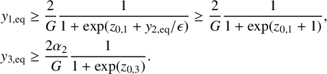 $$ \begin{align*} \begin{split} y_{1,\mathrm{eq}}&\geq\frac{2}{G}\frac{1}{1+\exp(z_{0,1}+y_{2,\mathrm{eq}}/\epsilon)}\geq \frac{2}{G}\frac{1}{1+\exp(z_{0,1}+1)},\\ y_{3,\mathrm{eq}}&\geq\frac{2\alpha_2}{G}\frac{1}{1+\exp(z_{0,3})}. \end{split} \end{align*} $$
Hence, for excitatory activation thresholds of order $\epsilon $
, the pair of small-
$\epsilon $
, the pair of small- $y_1$
equilibria does not exist. The other equilibria in Table 3 and Figure 3(h) have well-defined limits for
$y_1$
equilibria does not exist. The other equilibria in Table 3 and Figure 3(h) have well-defined limits for $y_{0,1}, y_{0,3}\to 0$
: the stable equilibrium has the limit
$y_{0,1}, y_{0,3}\to 0$
: the stable equilibrium has the limit $y_1=2/G$
, the unstable equilibrium has the limit
$y_1=2/G$
, the unstable equilibrium has the limit $y_1=y_{0,2}$
and its inhibitory activity
$y_1=y_{0,2}$
and its inhibitory activity $y_2$
approaches
$y_2$
approaches $2\alpha _2/G$
for small
$2\alpha _2/G$
for small $y_{0,1}$
. The saddle-node bifurcation at
$y_{0,1}$
. The saddle-node bifurcation at $\min (G_3,G_4)$
goes to infinity as
$\min (G_3,G_4)$
goes to infinity as $y_{0,1},y_{0,3}\to 0$
, such that the large-activity equilibrium exists over a wider range of G. This leaves the region
$y_{0,1},y_{0,3}\to 0$
, such that the large-activity equilibrium exists over a wider range of G. This leaves the region $(G_1,G_2)$
between the two Hopf bifurcations, where no stable equilibrium exists for
$(G_1,G_2)$
between the two Hopf bifurcations, where no stable equilibrium exists for $y_{0,1},y_{0,3}$
of order
$y_{0,1},y_{0,3}$
of order $\epsilon $
. The Hopf bifurcation at
$\epsilon $
. The Hopf bifurcation at $G_1$
has the limit
$G_1$
has the limit $\alpha _2b^*/\alpha _4$
for
$\alpha _2b^*/\alpha _4$
for $y_{0,1}\to 0$
, while
$y_{0,1}\to 0$
, while $G_2$
is independent of
$G_2$
is independent of $y_{0,1}$
and
$y_{0,1}$
and $y_{0,3}$
.
$y_{0,3}$
.
3.5 Periodic orbits in the small-
$\epsilon $
limit

3.5.1 The case
$\epsilon =0$
as a piecewise smooth ODE

System (3.2) in the limit $\epsilon \to 0$
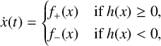
has discontinuities on the right-hand side such that it is only piecewise smooth in its phase space [Reference di Bernardo, Budd, Champneys and Kowalczyk9]. For such systems, there is, in general, no guarantee that trajectories can be consistently continued across discontinuities by following the flow defined by the right-hand sides in each part of the phase space. The problem can be illustrated for the simplest scenario, an ODE with a right-hand side consisting of two smooth pieces and a single discontinuity,
$\epsilon \to 0$
has discontinuities on the right-hand side such that it is only piecewise smooth in its phase space [Reference di Bernardo, Budd, Champneys and Kowalczyk9]. For such systems, there is, in general, no guarantee that trajectories can be consistently continued across discontinuities by following the flow defined by the right-hand sides in each part of the phase space. The problem can be illustrated for the simplest scenario, an ODE with a right-hand side consisting of two smooth pieces and a single discontinuity,
with smooth right-hand sides $f_\pm :{\mathbb {R}}^n\to {\mathbb {R}}^n$
and switching function
$f_\pm :{\mathbb {R}}^n\to {\mathbb {R}}^n$
and switching function $h:{\mathbb {R}}^n\to {\mathbb {R}}$
(for example, consider the scalar example
$h:{\mathbb {R}}^n\to {\mathbb {R}}$
(for example, consider the scalar example ![]() , where
, where $f_\pm (x)=\mp 1$
and
$f_\pm (x)=\mp 1$
and $h(x)=x$
). For all points with
$h(x)=x$
). For all points with $\pm h(x)>0$
, it is clear that the trajectory through x is determined by
$\pm h(x)>0$
, it is clear that the trajectory through x is determined by $f_\pm (x)$
. However, when following a trajectory
$f_\pm (x)$
. However, when following a trajectory $x(t)$
, one may approach a point x with
$x(t)$
, one may approach a point x with $h(x)=0$
(on the discontinuity surface
$h(x)=0$
(on the discontinuity surface $\{x\mid h(x)=0\}$
). If, in this point x, the quantities
$\{x\mid h(x)=0\}$
). If, in this point x, the quantities $h'(x)f_-(x)$
and
$h'(x)f_-(x)$
and $ h'(x)f_+(x)$
have opposite sign (using
$ h'(x)f_+(x)$
have opposite sign (using $h'(x)$
for
$h'(x)$
for $\partial h(x)$
), then the trajectory cannot “cross to the other side” of the discontinuity surface
$\partial h(x)$
), then the trajectory cannot “cross to the other side” of the discontinuity surface ${D=\{x\mid h(x)=0\}}$
consistent with the right-hand sides. A commonly adopted convention for this case where the flows on both sides of a codimension-
${D=\{x\mid h(x)=0\}}$
consistent with the right-hand sides. A commonly adopted convention for this case where the flows on both sides of a codimension- $1$
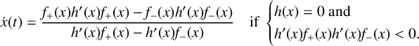
discontinuity surface point in opposite directions relative to the surface, is continuing the trajectory using the Filippov solution, or sliding, by following the flow of
$1$
discontinuity surface point in opposite directions relative to the surface, is continuing the trajectory using the Filippov solution, or sliding, by following the flow of
However, the structure of (3.2) rules out this common scenario of sliding, where $h'(x)f_+(x)h'(x)f_-(x)<0$
, for the discontinuity surfaces in system (3.2) generated by the limit
$h'(x)f_+(x)h'(x)f_-(x)<0$
, for the discontinuity surfaces in system (3.2) generated by the limit $\epsilon \to 0$
in (3.3). System (3.2) has three hyperplanes where it is discontinuous in the limit
$\epsilon \to 0$
in (3.3). System (3.2) has three hyperplanes where it is discontinuous in the limit $\epsilon \to 0$
, with the switching functions
$\epsilon \to 0$
, with the switching functions
In each of the hyperplanes $\{h_i=0\}$
, where the vector field is discontinuous, the two half-space vector fields point into the same direction relative to the hyperplane. This is due to the presence of inertia: (3.2) is a system of second-order equations for the firing activities, but the switches in
$\{h_i=0\}$
, where the vector field is discontinuous, the two half-space vector fields point into the same direction relative to the hyperplane. This is due to the presence of inertia: (3.2) is a system of second-order equations for the firing activities, but the switches in ${\mathrm {S}}_0$
depend only on the firing activities, not their time derivatives. Let us inspect each codimension-
${\mathrm {S}}_0$
depend only on the firing activities, not their time derivatives. Let us inspect each codimension- $1$
discontinuity set.
$1$
discontinuity set.
-
•
$D_i{\kern-1pt}={\kern-1pt}\{y{\kern-1pt}\mid{\kern-1pt} y_1{\kern-1pt}={\kern-1pt}y_{0,i}\}$
for
$i{\kern-1pt}={\kern-1pt}2,3$
, such that the switching function is : the inner product of the vector fields on both sides of
$D_i$
with the gradient of
$h_i$
equals , which is continuous across
$D_i$
and, thus, all nonequilibrium trajectories cross the surface
$D_i$
in the same direction from both sides of
$D_i$
. -
•
$D_1{\kern-1pt}={\kern-1pt}\{y{\kern-1pt}\mid{\kern-1pt} y_3-y_2{\kern-1pt}={\kern-1pt}y_{0,1}\}$
, such that the switching function is : the inner product of on both sides of
$D_1$
is , which is also continuous across
$D_1$
.


Hence, the set $\mathcal {D}$
in phase space where trajectories are not well defined in the classical sense is much smaller than for common piecewise smooth ODEs. It is a subset of the codimension-
$\mathcal {D}$
in phase space where trajectories are not well defined in the classical sense is much smaller than for common piecewise smooth ODEs. It is a subset of the codimension- $2$
surfaces
$2$
surfaces ![]() for
for $i=2,3$
and
$i=2,3$
and ![]() . Examples of points in these sets
. Examples of points in these sets $\mathcal {D}$
are the “unstable equilibria”
$\mathcal {D}$
are the “unstable equilibria” $y_{\mathrm {eq}_2}$
listed in Table 3. These types of equilibria are called pseudo equilibria in the literature about Filippov systems. As the equilibrium discussion in Figure 3 shows, the pseudo equilibria for
$y_{\mathrm {eq}_2}$
listed in Table 3. These types of equilibria are called pseudo equilibria in the literature about Filippov systems. As the equilibrium discussion in Figure 3 shows, the pseudo equilibria for $\epsilon =0$
are limits of unstable equilibria for
$\epsilon =0$
are limits of unstable equilibria for $\epsilon>0$
.
$\epsilon>0$
.
3.5.2 Numerical bifurcation analysis of
$\alpha $
-type periodic orbits for small positive
$\epsilon $


As seen in Table 3 and Figure 3(h), in the small- $\epsilon $
limit, the high-activity equilibrium
$\epsilon $
limit, the high-activity equilibrium $y_1$
changes not only its stability at
$y_1$
changes not only its stability at $G=G_1$
but also its location: the equilibrium pyramidal-cell activity drops sharply from
$G=G_1$
but also its location: the equilibrium pyramidal-cell activity drops sharply from $y_1=2/G=2/G_1\approx 1.35$
to
$y_1=2/G=2/G_1\approx 1.35$
to $y_1=y_{0,2}\approx 0.3$
. Hence, in the singular limit, we cannot expect the standard Hopf bifurcation scenario with a family of nearly harmonic small-amplitude periodic orbits branching off.
$y_1=y_{0,2}\approx 0.3$
. Hence, in the singular limit, we cannot expect the standard Hopf bifurcation scenario with a family of nearly harmonic small-amplitude periodic orbits branching off.
We initially perform a numerical continuation for the full nondimensionalized system (3.2) for small $\epsilon $
(
$\epsilon $
( $\epsilon =0.001$
). Figure 4 zooms into the range of parameters G where periodic orbits of
$\epsilon =0.001$
). Figure 4 zooms into the range of parameters G where periodic orbits of $\alpha $
type exist, near the Hopf bifurcation at
$\alpha $
type exist, near the Hopf bifurcation at $G=G_1\approx 1.48$
(see (3.10)). We observe that the pyramidal-cell (
$G=G_1\approx 1.48$
(see (3.10)). We observe that the pyramidal-cell ( $y_1$
) amplitude for the family of periodic orbits emerging from the Hopf bifurcation grows over a small range of G to order
$y_1$
) amplitude for the family of periodic orbits emerging from the Hopf bifurcation grows over a small range of G to order $1$
(black curve in top panel in Figure 4), by approximately the same amount as the equilibrium value of
$1$
(black curve in top panel in Figure 4), by approximately the same amount as the equilibrium value of $y_1$
dropped before the Hopf bifurcation. This explosive growth in amplitude is reminiscent of canard explosions as first described for the classical van der Pol or FitzHugh–Nagumo oscillator by Benoît [Reference Benoît, Callot, Diener and Diener2] (see Krupa and Szmolyan [Reference Krupa and Szmolyan18] for general theory and Wechselberger [Reference Wechselberger28] for a review). However, the inhibition amplitude
$y_1$
dropped before the Hopf bifurcation. This explosive growth in amplitude is reminiscent of canard explosions as first described for the classical van der Pol or FitzHugh–Nagumo oscillator by Benoît [Reference Benoît, Callot, Diener and Diener2] (see Krupa and Szmolyan [Reference Krupa and Szmolyan18] for general theory and Wechselberger [Reference Wechselberger28] for a review). However, the inhibition amplitude $y_2$
grows square-root-like with
$y_2$
grows square-root-like with $G-G_1$
, as occurs at a classical Hopf bifurcation. This discrepancy and the fact that the singular limit
$G-G_1$
, as occurs at a classical Hopf bifurcation. This discrepancy and the fact that the singular limit $\epsilon \to 0$
is not slow–fast but discontinuous suggests that another mechanism must be responsible for the explosive growth in amplitude of
$\epsilon \to 0$
is not slow–fast but discontinuous suggests that another mechanism must be responsible for the explosive growth in amplitude of $y_1$
. Exploration of this phenomenon is beyond the scope of this paper. The time profile of periodic orbits near the explosion is shown in Figure 7 in the discussion in Section 4.
$y_1$
. Exploration of this phenomenon is beyond the scope of this paper. The time profile of periodic orbits near the explosion is shown in Figure 7 in the discussion in Section 4.
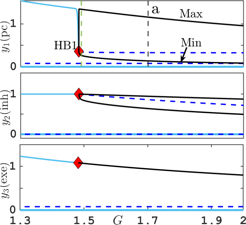
Figure 4 Equilibria and periodic orbits branching off Hopf bifurcation (HB1) for system (3.2) for varying G and small $\epsilon =0.001$
, showing equilibrium values, or maxima and minima of the neural activities
$\epsilon =0.001$
, showing equilibrium values, or maxima and minima of the neural activities $y_1,y_2,y_3$
, respectively. Green vertical line corresponds to canard orbit shown in Figure 7. Grey vertical line is at parameter
$y_1,y_2,y_3$
, respectively. Green vertical line corresponds to canard orbit shown in Figure 7. Grey vertical line is at parameter $G=1.7$
, used in singular limit in Figure 5(a). Other parameters are listed in Table 2.
$G=1.7$
, used in singular limit in Figure 5(a). Other parameters are listed in Table 2.
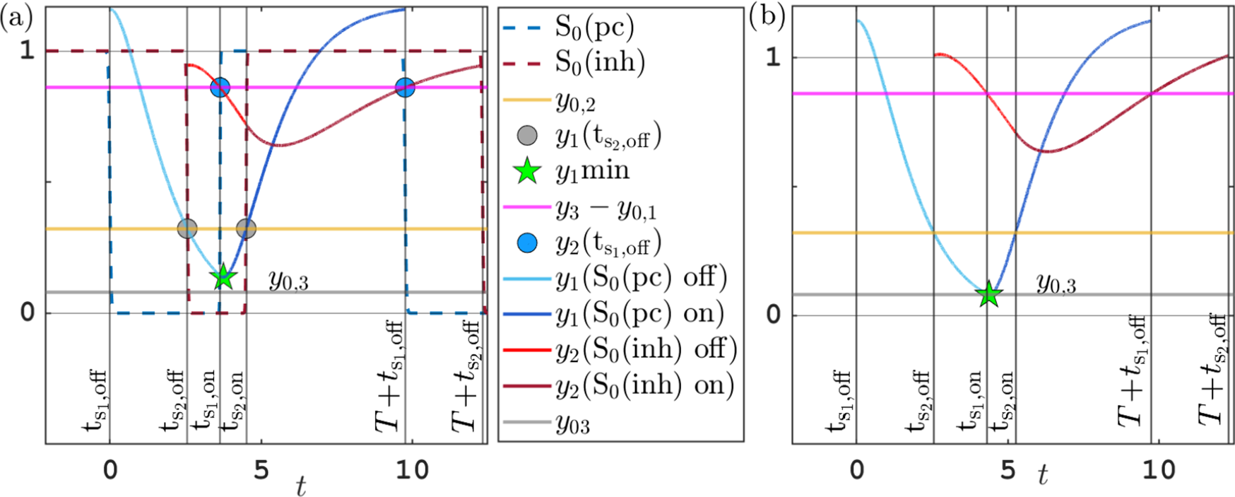
Figure 5 Time profile of alpha-type piecewise exponential periodic orbits given in (3.15), representing solutions of the piecewise linear ODE (3.12), (3.13) for $y_{0,1},y_{0,3}=0.08$
,
$y_{0,1},y_{0,3}=0.08$
, $y_{0,2}=0.3$
and
$y_{0,2}=0.3$
and $y_3$
fixed at its equilibrium value
$y_3$
fixed at its equilibrium value $2\alpha _2/G$
. (a) Orbit for
$2\alpha _2/G$
. (a) Orbit for $(b^*,G)=(0.5,1.7)$
;
$(b^*,G)=(0.5,1.7)$
; $t_{\mathrm {s_2,off}}$
,
$t_{\mathrm {s_2,off}}$
, $t_{\mathrm {s_2,on}}$
: threshold crossing times of
$t_{\mathrm {s_2,on}}$
: threshold crossing times of $y_1$
(where
$y_1$
(where $y_1=y_{0,2}$
);
$y_1=y_{0,2}$
); $t_{\mathrm {s_1,off}}$
,
$t_{\mathrm {s_1,off}}$
, $t_{\mathrm {s_1,on}}$
: threshold crossing times of
$t_{\mathrm {s_1,on}}$
: threshold crossing times of $y_2$
(where
$y_2$
(where $y_2=y_3-y_{0,1}$
). Dashed blue line (legend entry
$y_2=y_3-y_{0,1}$
). Dashed blue line (legend entry $S_0$
(pc)) is activation switch
$S_0$
(pc)) is activation switch ${\mathrm {S}}_{0}(y_3-y_2(t)-y_{0,1})$
for
${\mathrm {S}}_{0}(y_3-y_2(t)-y_{0,1})$
for $y_1$
with
$y_1$
with $\epsilon =0.001$
. Dashed red line (legend entry
$\epsilon =0.001$
. Dashed red line (legend entry $S_0$
(inh)) is activation switch
$S_0$
(inh)) is activation switch ${\mathrm {S}}_{0}(y_1(t)-y_{0,2})$
for
${\mathrm {S}}_{0}(y_1(t)-y_{0,2})$
for $y_2$
. (b) Same as panel (a) but for
$y_2$
. (b) Same as panel (a) but for $(b^*,G)=(0.44,1.7)$
, where orbit grazes (
$(b^*,G)=(0.44,1.7)$
, where orbit grazes ( $y_{1,\min }=y_{0,3}$
, green star on grey horizontal line
$y_{1,\min }=y_{0,3}$
, green star on grey horizontal line $\{y=y_{0,3}\}$
). For other parameters, see Table 2.
$\{y=y_{0,3}\}$
). For other parameters, see Table 2.
3.5.3 Piecewise linear oscillations in a negative feedback loop between pyramidal cells and inhibition for
$\epsilon =0$

In Figure 4, we also note that for $G\approx G_1$
and pyramidal-cell activity
$G\approx G_1$
and pyramidal-cell activity $y_1$
in the range between
$y_1$
in the range between $y_{0,2}$
and
$y_{0,2}$
and $2/G_1$
, the excitatory interneurons are uniformly active, as
$2/G_1$
, the excitatory interneurons are uniformly active, as $y_1$
is always above the threshold
$y_1$
is always above the threshold $y_{0,3}$
at which excitatory interneuron activity is switched off, and which is much smaller than
$y_{0,3}$
at which excitatory interneuron activity is switched off, and which is much smaller than $y_{0,2}$
. Hence,
$y_{0,2}$
. Hence, $y_3$
will be positive and at its equilibrium value
$y_3$
will be positive and at its equilibrium value
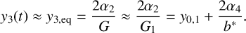 $$ \begin{align*} y_3(t)\approx y_{3,\mathrm{eq}}=\frac{2\alpha_2}{G}\approx \frac{2\alpha_2}{G_1}= y_{0,1}+\frac{2\alpha_4}{b^*}. \end{align*} $$
Thus, we may replace $y_3$
in the sigmoid input for
$y_3$
in the sigmoid input for $y_1$
with its equilibrium value, resulting in the four-dimensional system for pyramidal-cell and inhibitory activity only, inserting the limit
$y_1$
with its equilibrium value, resulting in the four-dimensional system for pyramidal-cell and inhibitory activity only, inserting the limit $\epsilon =0$
:
$\epsilon =0$
:
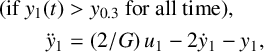
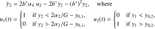
System (3.12), (3.13) is a classical negative feedback loop with inertia: $y_2$
suppresses
$y_2$
suppresses $y_1$
, while
$y_1$
, while $y_1$
promotes
$y_1$
promotes $y_2$
. Each oscillation period has four phases and follows a piecewise linear second-order vector field in each of the phases.
$y_2$
. Each oscillation period has four phases and follows a piecewise linear second-order vector field in each of the phases.
Figure 5(a) shows the typical shape for the $y_1$
and
$y_1$
and $y_2$
profile of the oscillations. We reduce the periodic problem for the four-dimensional piecewise affine ODE to a four-dimensional algebraic problem, parametrizing the oscillations using the times at which the respective activations
$y_2$
profile of the oscillations. We reduce the periodic problem for the four-dimensional piecewise affine ODE to a four-dimensional algebraic problem, parametrizing the oscillations using the times at which the respective activations $u_1, u_2$
switch between
$u_1, u_2$
switch between $0$
and
$0$
and $1$
(without loss of generality
$1$
(without loss of generality $t_{\mathrm {s_1,off}}=0$
), (see Figure 5(a) for guidance):
$t_{\mathrm {s_1,off}}=0$
), (see Figure 5(a) for guidance):
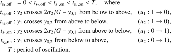 $$ \begin{align*} \begin{aligned} t_{\mathrm{s_1,off}}\phantom{:}\ &=0<t_{\mathrm{s_2,off}}<t_{\mathrm{s_1,on}}<t_{\mathrm{s_2,on}}<T,\quad \text{where}\\ t_{\mathrm{s_1,off}}:&\ y_2\text{ crosses }2\alpha_2/G-y_{0,1}\text{ from below to above,}&&\text{(}u_1:1\to0\text{),}\\ t_{\mathrm{s_2,off}}:&\ y_1\text{ crosses }y_{0,2}\text{ from above to below,}&&\text{(}u_2:1\to0\text{),}\\ t_{\mathrm{s_1,on}}:&\ y_2\text{ crosses }2\alpha_2/G-y_{0,1}\text{ from above to below,}&&\text{(}u_1:0\to1\text{),}\\ t_{\mathrm{s_2,on}}:&\ y_1\text{ crosses }y_{0,2}\text{ from below to above,}&&\text{(}u_2:0\to1\text{),}\\ T:&\ \text{period of oscillation.} \end{aligned} \end{align*} $$
3.5.4 Alpha-type oscillations in the singular limit
For $G>G_1$
, the periodic orbits consist of two coupled pairs of orbit segments, one pair of segments for pyramidal activity
$G>G_1$
, the periodic orbits consist of two coupled pairs of orbit segments, one pair of segments for pyramidal activity $y_1$
governed by the piecewise linear ODE (3.12) (switching at times
$y_1$
governed by the piecewise linear ODE (3.12) (switching at times $t_{\mathrm {s_1,off}}$
and
$t_{\mathrm {s_1,off}}$
and $t_{\mathrm {s_1,on}})$
and one pair of segments for inhibition
$t_{\mathrm {s_1,on}})$
and one pair of segments for inhibition $y_2$
governed by the piecewise linear ODE (3.13) (switching at times
$y_2$
governed by the piecewise linear ODE (3.13) (switching at times $t_{\mathrm {s_2,off}}$
and
$t_{\mathrm {s_2,off}}$
and $t_{\mathrm {s_2,on}}$
), as shown in Figure 5(a). The coupling occurs through the switching times, as the switching times
$t_{\mathrm {s_2,on}}$
), as shown in Figure 5(a). The coupling occurs through the switching times, as the switching times $t_{\mathrm {s_2,on/off}}$
are determined by
$t_{\mathrm {s_2,on/off}}$
are determined by $y_1$
crossing the threshold
$y_1$
crossing the threshold $y_{0,2}$
, and the switching times
$y_{0,2}$
, and the switching times $t_{\mathrm {s_1,on/off}}$
are determined by
$t_{\mathrm {s_1,on/off}}$
are determined by $y_2$
crossing the threshold
$y_2$
crossing the threshold $y_{\mathrm {3,eq}}-y_{0,1}=2\alpha _2/G-y_{0,1}$
. Both piecewise linear ODEs (3.12) and (3.13) are affine ODEs of the form
$y_{\mathrm {3,eq}}-y_{0,1}=2\alpha _2/G-y_{0,1}$
. Both piecewise linear ODEs (3.12) and (3.13) are affine ODEs of the form
with inhomogeneity c. The general solution ![]() of (3.14) for its IVP with initial condition
of (3.14) for its IVP with initial condition ![]() is
is
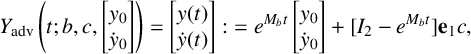
 $$ \begin{align*} \text{where} \quad e^{M_bt}&=e^{-bt}\begin{bmatrix} 1+bt&t\\ -b^2t&1-bt \end{bmatrix}, \end{align*} $$ $e^{(\cdot )}$
is the exponential and
$e^{(\cdot )}$
is the exponential and $\mathbf {{e}}_1=(1,0)^{\mathsf {T}}$
is the first standard basis vector. From this general formula, we find that requiring periodicity of the pyramidal activity
$\mathbf {{e}}_1=(1,0)^{\mathsf {T}}$
is the first standard basis vector. From this general formula, we find that requiring periodicity of the pyramidal activity $y_1$
and the inhibition
$y_1$
and the inhibition $y_2$
determines their initial conditions at the “off” switching time. The initial conditions
$y_2$
determines their initial conditions at the “off” switching time. The initial conditions
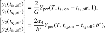
where $Y_{\mathrm {per}}$
is defined as
$Y_{\mathrm {per}}$
is defined as
 $$ \begin{align*}Y_{\mathrm{per}}(T,\delta_t;b)=[I_2-e^{M_bT}]^{-1}[I_2-e^{M_b(T-\delta_t)}]\mathbf{{e}}_1,\end{align*} $$
will lead to a solution of (3.12), (3.13) that is periodic with period T. The switching times $t_{\mathrm {s_1,on}}$
,
$t_{\mathrm {s_1,on}}$
, $t_{\mathrm {s_2,on/off}}$
and the period T satisfy four relations that follow from the crossing conditions
$t_{\mathrm {s_2,on/off}}$
and the period T satisfy four relations that follow from the crossing conditions $y_1( t_{\mathrm {s_2,off}})=y_1( t_{\mathrm {s_2,on}})=y_{02}$
and
$y_1( t_{\mathrm {s_2,off}})=y_1( t_{\mathrm {s_2,on}})=y_{02}$
and $y_2( t_{\mathrm {s_1,off}})=y_2( t_{\mathrm {s_1,on}})=y_3-y_{01}$
:
$y_2( t_{\mathrm {s_1,off}})=y_2( t_{\mathrm {s_1,on}})=y_3-y_{01}$
:
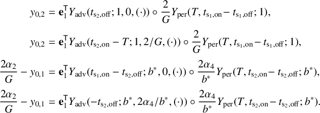 $$ \begin{align} \begin{aligned} y_{0,2}&=\mathbf{{e}}_1^{\mathsf{T}} Y_{\mathrm{adv}}(t_{\mathrm{s_2,off}}; 1,0, (\cdot))\circ\frac{2}{G}Y_{\mathrm{per}}(T,t_{\mathrm{s_1,on}}\!-t_{\mathrm{s_1,off}};1),\\[0.1cm] y_{0,2}&=\mathbf{{e}}_1^{\mathsf{T}} Y_{\mathrm{adv}}(t_{\mathrm{s_2,on}}-T;1,2/G, (\cdot))\circ\frac{2}{G}Y_{\mathrm{per}}(T,t_{\mathrm{s_1,on}}\!-t_{\mathrm{s_1,off}};1),\\[0.1cm] \frac{2\alpha_2}{G}-y_{0,1}&=\mathbf{{e}}_1^{\mathsf{T}} Y_{\mathrm{adv}}(t_{\mathrm{s_1,on}}-t_{\mathrm{s_2,off}};b^*,0,(\cdot))\circ\frac{2\alpha_4}{b^*} Y_{\mathrm{per}}(T,t_{\mathrm{s_2,on}}\!-t_{\mathrm{s_2,off}};b^*),\\[0.1cm] \frac{2\alpha_2}{G}-y_{0,1}&=\mathbf{{e}}_1^{\mathsf{T}} Y_{\mathrm{adv}}(-t_{\mathrm{s_2,off}};b^*,2\alpha_4/b^*,(\cdot))\circ\frac{2\alpha_4}{b^*} Y_{\mathrm{per}}(T,t_{\mathrm{s_2,on}}\!-t_{\mathrm{s_2,off}};b^*). \end{aligned} \end{align} $$
In (3.15) and below, we use the composition symbol $\circ $
with the meaning
$\circ $
with the meaning $f\circ x=f(x)$
,
$f\circ x=f(x)$
, $f\circ g\circ x=f(g(x))$
and so forth to reduce nesting of brackets. Recall that we set
$f\circ g\circ x=f(g(x))$
and so forth to reduce nesting of brackets. Recall that we set $t_{\mathrm {s_1,off}}=0$
such that this switching time has been omitted in the defining equations (3.15). We have already inserted the appropriate initial conditions to ensure periodicity with period T into (3.15), such that the system (3.15) is a system of four algebraic equations, depending on the four unknown times
$t_{\mathrm {s_1,off}}=0$
such that this switching time has been omitted in the defining equations (3.15). We have already inserted the appropriate initial conditions to ensure periodicity with period T into (3.15), such that the system (3.15) is a system of four algebraic equations, depending on the four unknown times $t_{\mathrm {s_1,on}}$
,
$t_{\mathrm {s_1,on}}$
, $t_{\mathrm {s_2,off}}$
,
$t_{\mathrm {s_2,off}}$
, $t_{\mathrm {s_2,on}}$
and T, and system parameters such as G,
$t_{\mathrm {s_2,on}}$
and T, and system parameters such as G, $b^*$
and the switching thresholds
$b^*$
and the switching thresholds $y_{0,1},y_{0,2}$
. For given switching times and period, one may obtain the complete periodic orbit as
$y_{0,1},y_{0,2}$
. For given switching times and period, one may obtain the complete periodic orbit as
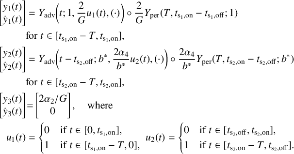
Figure 5(a) shows an example of such a piecewise exponential and its switching times. The associated thresholds $y_{\mathrm {3,eq}}-y_{0,1}=2\alpha _2/G-y_{0,1}$
and
$y_{\mathrm {3,eq}}-y_{0,1}=2\alpha _2/G-y_{0,1}$
and $y_{0,2}$
for
$y_{0,2}$
for $y_2(t)$
and
$y_2(t)$
and $y_1(t)$
for the switching events of
$y_1(t)$
for the switching events of $y_1(t)$
and
$y_1(t)$
and $y_2(t)$
are shown as magenta and yellow horizontal lines, respectively.
$y_2(t)$
are shown as magenta and yellow horizontal lines, respectively.
3.5.5 Detection of grazing boundary for alpha activity
The orbits given by the algebraic system (3.15) are alpha-type oscillations with constant support by excitatory interneuron population $y_3$
. A criterion for the existence of these oscillations is that
$y_3$
. A criterion for the existence of these oscillations is that $y_1$
never crosses below the threshold
$y_1$
never crosses below the threshold $y_{0,3}$
at which the excitatory interneurons
$y_{0,3}$
at which the excitatory interneurons $y_3$
switch off. The piecewise exponential has a distinct minimum
$y_3$
switch off. The piecewise exponential has a distinct minimum $y_{1,\min }$
at some time
$y_{1,\min }$
at some time $t_{1,\min }$
, labelled by a star in Figure 5(a). This minimum consistently occurs shortly after
$t_{1,\min }$
, labelled by a star in Figure 5(a). This minimum consistently occurs shortly after $t_{\mathrm {s_1,on}}$
, in the interval between
$t_{\mathrm {s_1,on}}$
, in the interval between $t_{\mathrm {s_1,on}}$
and
$t_{\mathrm {s_1,on}}$
and $t_{\mathrm {s_2,on}}$
, due to the inertia caused by the second-order nature of the ODE for
$t_{\mathrm {s_2,on}}$
, due to the inertia caused by the second-order nature of the ODE for $y_1$
. Hence, we may introduce
$y_1$
. Hence, we may introduce $y_{1,\min }$
and
$y_{1,\min }$
and $t_{1,\min }$
as additional parameters satisfying the relations
$t_{1,\min }$
as additional parameters satisfying the relations
 $$ \begin{align} \begin{bmatrix} y_{1,\min}\\0 \end{bmatrix}&= Y_{\mathrm{adv}}(t_{1,\min}-t_{\mathrm{s_1,on}};1,2/G,(\cdot))\circ Y_{\mathrm{adv}}(t_{\mathrm{s_1,on}};1,0,(\cdot)) \notag \\ &\quad \circ (2/G)Y_{\mathrm{per}}(T,t_{\mathrm{s_1,on}}-t_{\mathrm{s_1,off}};1). \end{align} $$
We add the two parameters $t_{1,\min }$
and
$t_{1,\min }$
and $y_{1,\min }$
while tracking solutions of (3.15), (3.16) in system parameters to monitor the difference
$y_{1,\min }$
while tracking solutions of (3.15), (3.16) in system parameters to monitor the difference $y_{1,\min }-y_{0,3}$
for roots. The difference equals the distance between the point on the graph in Figure 5(a) labelled with a star and the grey horizontal line
$y_{1,\min }-y_{0,3}$
for roots. The difference equals the distance between the point on the graph in Figure 5(a) labelled with a star and the grey horizontal line $D_3=\{y_1=y_{0,3}\}$
. When this difference is zero, we have a grazing bifurcation: the alpha activity oscillation’s orbit touches the threshold
$D_3=\{y_1=y_{0,3}\}$
. When this difference is zero, we have a grazing bifurcation: the alpha activity oscillation’s orbit touches the threshold $D_3=\{y\mid y_1=y_{0,3}\}$
in a quadratic tangency. To find an orbit with such a quadratic tangency, we fix
$D_3=\{y\mid y_1=y_{0,3}\}$
in a quadratic tangency. To find an orbit with such a quadratic tangency, we fix $G=1.7$
and vary the time scale ratio
$G=1.7$
and vary the time scale ratio $b^*$
from
$b^*$
from $b^*=0.5$
downwards along the horizontal dashed line shown in Figure 6(a). While doing so, we monitor the quantity
$b^*=0.5$
downwards along the horizontal dashed line shown in Figure 6(a). While doing so, we monitor the quantity $y_{1,\min }-y_{0,3}$
until it reaches zero, which is the point that represents the grazing bifurcation. The grazing occurs at
$y_{1,\min }-y_{0,3}$
until it reaches zero, which is the point that represents the grazing bifurcation. The grazing occurs at $(b^*,G)\approx (0.44,1.7)$
, labelled with a green star in Figure 6(a).
$(b^*,G)\approx (0.44,1.7)$
, labelled with a green star in Figure 6(a).
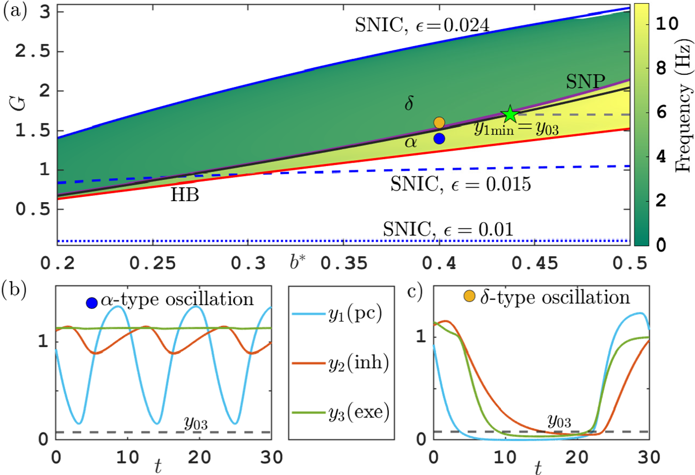
Figure 6 (a) Composite bifurcation diagram overlaying regions of alpha and delta activity of system (3.2) for $\epsilon =0.024$
, and the grazing bifurcation (black curve) detected by solving algebraic equations (3.15), (3.16) in the
$\epsilon =0.024$
, and the grazing bifurcation (black curve) detected by solving algebraic equations (3.15), (3.16) in the $(b^*,G)$
parameter plane. (b,c) Time profiles of typical alpha activity (
$(b^*,G)$
parameter plane. (b,c) Time profiles of typical alpha activity ( $(b^*,G)=(0.4,1.4)$
, blue circle in panel (a)) and delta activity (
$(b^*,G)=(0.4,1.4)$
, blue circle in panel (a)) and delta activity ( $(b^*,G)=(0.4,1.6)$
, yellow circle in panel (a)) for each neuron population at
$(b^*,G)=(0.4,1.6)$
, yellow circle in panel (a)) for each neuron population at $\epsilon =0.024$
. Folds of periodic orbit (SNP, two purple curves on top of each other) and Hopf bifurcation (HB, red) are for
$\epsilon =0.024$
. Folds of periodic orbit (SNP, two purple curves on top of each other) and Hopf bifurcation (HB, red) are for $\epsilon =0.024$
, SNIC bifurcations are shown for
$\epsilon =0.024$
, SNIC bifurcations are shown for $\epsilon =0.024,0.015,0.01$
. Horizontal grey dashed line for
$\epsilon =0.024,0.015,0.01$
. Horizontal grey dashed line for $b^*\in [0.44,0.5]$
at
$b^*\in [0.44,0.5]$
at $G=1.7$
is the parameter path for continuation to grazing bifurcation reached at the point labelled by a green star. See Table 2 for other parameters.
$G=1.7$
is the parameter path for continuation to grazing bifurcation reached at the point labelled by a green star. See Table 2 for other parameters.
3.5.6 Mapping alpha and delta oscillations: a two-parameter bifurcation analysis
Following detection of this grazing bifurcation at $(b^*,G)\approx (0.44,1.7)$
, we track its locus in two system parameters, time scale ratio
$(b^*,G)\approx (0.44,1.7)$
, we track its locus in two system parameters, time scale ratio $b^*$
and the feedback ratio G, by imposing the algebraic condition
$b^*$
and the feedback ratio G, by imposing the algebraic condition $y_{1,\min }-y_{0,3}=0$
. The resulting curve in the
$y_{1,\min }-y_{0,3}=0$
. The resulting curve in the $(b^*,G)$
-plane is shown in Figure 6(a) in black. We combine this curve with the other relevant bifurcations bounding alpha and delta activity:
$(b^*,G)$
-plane is shown in Figure 6(a) in black. We combine this curve with the other relevant bifurcations bounding alpha and delta activity:
-
(1) (Hopf bifurcation) The Hopf bifurcation curve is the lower bound for alpha activity in G. It is given by (3.10) in the limit
$\epsilon =0$
(
$G_1=\alpha _2 b^*/(\alpha _4+y_{0,1}b^*/2)$
) and shown in red in Figure 6(a) for
$\epsilon =0.024$
. The value
$\epsilon =0.024$
is the original value of
$\epsilon $
given in Table 2. Visually, the Hopf curve for
$\epsilon =0.024$
is indistinguishable from its
$\epsilon =0$
limit. -
(2) (Grazing bifurcation) Asymptotically for
$\epsilon \to 0$
, the transition boundary between delta and alpha activity is the grazing curve determined by the algebraic equations (3.15), (3.16), shown in black in Figure 6(a). -
(3) (SNIC bifurcation) The upper bound in G for
$\delta $
activity is a SNIC bifurcation, determined by the saddle-node of equilibria for the stable small-activity equilibrium, labelled
$y_{\mathrm {eq}_1}$
, and the small-activity saddle
$y_{\mathrm {eq}_2}$
in Table 3. Table 3 indicates that both equilibria exist for all positive values of G for
$\epsilon =0$
and (uniformly in
$\epsilon $
) positive thresholds
$y_{0,1}$
and
$y_{0,3}$
. Hence, the parameter value
$G_{\mathrm {SNIC}}$
for the SNIC bifurcation shown in Figure 2(c) has the limit
$G_{\mathrm {SNIC}}\to 0$
for
$\epsilon \to 0$
. We included the SNIC bifurcation curve for three values of
$\epsilon $
(the original value
$0.024$
given in Table 2,
$0.015$
and
$0.01$
) in Figure 6(a) to visualize the effect of decreasing
$\epsilon $
. For
$(b^*,G)$
above the SNIC bifurcation curve, the activity drops to its small-activity equilibrium.


To demonstrate the quantitative accuracy of the prediction from the singular limit $\epsilon =0$
for the transition between delta and alpha activity, we include shading according to frequency in areas where we find oscillations for the positive value
$\epsilon =0$
for the transition between delta and alpha activity, we include shading according to frequency in areas where we find oscillations for the positive value $\epsilon =0.024$
from Table 2. We observe a sharp drop in frequency for increasing G near the singular-limit grazing bifurcation (from yellow to green in Figure 6(a)). Panels (b) and (c) in Figure 6 show time profiles at representative points in the alpha region (
$\epsilon =0.024$
from Table 2. We observe a sharp drop in frequency for increasing G near the singular-limit grazing bifurcation (from yellow to green in Figure 6(a)). Panels (b) and (c) in Figure 6 show time profiles at representative points in the alpha region ( $(b^*,G)=(0.4,0.14)$
, blue circle) and in the delta region (
$(b^*,G)=(0.4,0.14)$
, blue circle) and in the delta region ( $(b^*,G)=(0.4,0.16)$
, yellow circle). For larger
$(b^*,G)=(0.4,0.16)$
, yellow circle). For larger $b^*$
, a small deviation is noticeable such that the effect of nonzero
$b^*$
, a small deviation is noticeable such that the effect of nonzero $\epsilon $
is slightly larger near
$\epsilon $
is slightly larger near $b^*\approx 0.5$
. The pair of folds of periodic orbits which coincides with the frequency drop (see Figures 2(b) and 2(c) is also included for
$b^*\approx 0.5$
. The pair of folds of periodic orbits which coincides with the frequency drop (see Figures 2(b) and 2(c) is also included for $\epsilon =0.024$
as a pair of purple curves, labelled SNP (the two SNP curves are close to each other, such that one obscures the other). The pair of folds overlaps with the grazing bifurcation for
$\epsilon =0.024$
as a pair of purple curves, labelled SNP (the two SNP curves are close to each other, such that one obscures the other). The pair of folds overlaps with the grazing bifurcation for $\epsilon =0$
over large parts of the parameter plane.
$\epsilon =0$
over large parts of the parameter plane.
4 Discussion and further analysis
We have identified the mechanism responsible for the transition between alpha- and delta-type activity in the Jansen–Rit model [Reference Jansen and Rit16]. The transition between alpha-type oscillations and delta-type oscillations in neural circuits is relevant to applications because alpha frequencies are associated with the promotion of long-term potentiation (LTP), enhancing synaptic strength and facilitating memory formation during active learning, while delta frequencies are associated with long-term depression (LTD), which promotes synaptic weakening and neural plasticity during deep sleep [Reference Rashmii24]. The combined effects of these processes contribute to learning via consolidation of memory across the wakefulness and sleep cycles [Reference Brudzynski, Burgdorf and Moskal3, Reference Burgdorf and Moskal4]. Therefore, understanding these transitions enhances our knowledge of how neural circuits regulate brain states and may provide insights into disruptions that affect sleep and cognitive functions. In the Jansen–Rit model, the transition is not associated with one of the generic codimension-one bifurcations, but it occurs over a small range of parameter values for decreasing excitatory feedback strength A and with little to no hysteresis. In the transition, the time profile and the frequency change sharply: oscillations during alpha activity show a shape typical for a single negative feedback loop because of the near-constant support from the excitatory interneurons. Oscillations during delta activity are of relaxation type with long periods of near-zero activity (see Figures 2(d) and 2(e) in Section 2). The feedback strength parameter A affects how neurons respond to incoming signals by scaling the excitable population’s output of firing rates [Reference Jansen and Rit16].
The results presented in Section 3 show that the singular limit where one assumes that the activation is an all-or-nothing switch reduces the sharp transition in shape and frequency to a grazing bifurcation: when the pyramidal-cell activity “touches” the threshold line for switching off the excitatory interneurons in a quadratic tangency, the excitatory interneuron activity collapses. This causes a further drop of pyramidal-cell activity, such that both populations approach near-zero activity. They stay there until the (slower) inhibition activity has dropped sufficiently low to permit recovery of excitatory activity in pyramidal and interneuron populations (that is, neuron response to incoming signals acts as binary operation off/on) in Section 3. The singular limit allow us to detect the curve of grazing bifurcation separating the two distinct wave rhythms (that is, the boundary between two distinct types of periodic orbits) in the two parameter plane $(b^*,G)$
, where
$(b^*,G)$
, where $b^*$
is the decay rate ratio of inhibitory to excitatory populations and G is the ratio of postsynaptic amplitudes of inhibitory to excitatory populations in nondimensionalized model (3.2).
$b^*$
is the decay rate ratio of inhibitory to excitatory populations and G is the ratio of postsynaptic amplitudes of inhibitory to excitatory populations in nondimensionalized model (3.2).
There are several further open questions for the analysis of the singular limit.
4.0.1 Small-threshold analysis of alpha–delta transition and SNIC
Our analysis shows that the limit $\epsilon \to 0$
with fixed thresholds
$\epsilon \to 0$
with fixed thresholds $y_{0,1}$
,
$y_{0,1}$
, $y_{0,3}$
does not support delta-type oscillations. In delta-type oscillations, all potentials come close to zero such that these oscillations are only possible if there are no stable equilibria at small
$y_{0,3}$
does not support delta-type oscillations. In delta-type oscillations, all potentials come close to zero such that these oscillations are only possible if there are no stable equilibria at small $y_1$
,
$y_1$
, $y_3$
. However, Figure 6 shows that for all sufficiently small
$y_3$
. However, Figure 6 shows that for all sufficiently small $\epsilon $
, there are no parameter values
$\epsilon $
, there are no parameter values $(b^*,G)$
for which grazing has happened (so, above the black curve) but no equilibria with
$(b^*,G)$
for which grazing has happened (so, above the black curve) but no equilibria with $y_1\approx 0$
,
$y_1\approx 0$
, $y_3\approx 0$
exist (below the blue solid/dashed/dotted curve called SNIC). This is because for positive
$y_3\approx 0$
exist (below the blue solid/dashed/dotted curve called SNIC). This is because for positive $y_{0,1}$
,
$y_{0,1}$
, $y_{0,3}$
and small
$y_{0,3}$
and small $y_1$
,
$y_1$
, $y_2$
,
$y_2$
, $y_3$
, the existing stable “off” equilibrium
$y_3$
, the existing stable “off” equilibrium $y_{\mathrm {eq}_1}$
from Table 3 attracts trajectories with
$y_{\mathrm {eq}_1}$
from Table 3 attracts trajectories with $y_1,y_2,y_3\approx 0$
. If we also consider the thresholds for the excitatory populations as small quantities, then delta-type oscillations are possible for small
$y_1,y_2,y_3\approx 0$
. If we also consider the thresholds for the excitatory populations as small quantities, then delta-type oscillations are possible for small $\epsilon $
: as we showed in Section 3.3, if the thresholds are proportional to
$\epsilon $
: as we showed in Section 3.3, if the thresholds are proportional to $\epsilon $
, then there are no small equilibria present for small
$\epsilon $
, then there are no small equilibria present for small $\epsilon $
. A more detailed analysis is needed to find for which asymptotic order of magnitude for the thresholds a saddle-node (and, hence, SNIC) is present for parameters G of order
$\epsilon $
. A more detailed analysis is needed to find for which asymptotic order of magnitude for the thresholds a saddle-node (and, hence, SNIC) is present for parameters G of order $1$
.
$1$
.
The expressions in (3.15) show that the dependence of the alpha-type periodic orbits on the threshold $y_{0,1}$
is regular, such that replacing
$y_{0,1}$
is regular, such that replacing $y_{0,1}$
by zero in (3.15) will not have a large effect. However, the grazing bifurcation is determined by the minimum of
$y_{0,1}$
by zero in (3.15) will not have a large effect. However, the grazing bifurcation is determined by the minimum of $y_1$
reaching
$y_1$
reaching $y_{0,3}$
, such that for
$y_{0,3}$
, such that for $y_{0,3}\to 0$
, the grazing bifurcation will shift. The pyramidal-cell potential
$y_{0,3}\to 0$
, the grazing bifurcation will shift. The pyramidal-cell potential $y_1$
decays exponentially as long as the inhibition
$y_1$
decays exponentially as long as the inhibition $y_2$
is above the equilibrium value of the threshold
$y_2$
is above the equilibrium value of the threshold $y_3-y_{0,1}\approx 2\alpha _2/G$
. As a smaller
$y_3-y_{0,1}\approx 2\alpha _2/G$
. As a smaller $b^*$
leads to a slow-down in the change of inhibition
$b^*$
leads to a slow-down in the change of inhibition $y_2$
, a decrease of
$y_2$
, a decrease of $b^*$
leads to a longer period of exponential decay for
$b^*$
leads to a longer period of exponential decay for $y_1$
, so to a smaller minimum of
$y_1$
, so to a smaller minimum of $y_1$
. Hence, we expect the value of
$y_1$
. Hence, we expect the value of $b^*$
for the grazing bifurcation to decrease slowly with
$b^*$
for the grazing bifurcation to decrease slowly with $\epsilon $
, on the order of
$\epsilon $
, on the order of $1/|\kern-1.3pt\log \epsilon |$
, because of the exponential decay of
$1/|\kern-1.3pt\log \epsilon |$
, because of the exponential decay of $y_1$
for above threshold inhibition.
$y_1$
for above threshold inhibition.
4.1 Canard explosion of alpha-type orbits at the singular Hopf bifurcation
The Hopf bifurcation, shown in the zoomed-in bifurcation diagram in Figure 4 can be studied in the singular limit $\epsilon =0$
. Figure 7 shows that the periodic orbits in this canard-like explosion are parametrized by the time during which inhibition is switched off (drop of dashed curve in Figure 7(b) to zero), which is short for values of the parameter G close to the bifurcation value
$\epsilon =0$
. Figure 7 shows that the periodic orbits in this canard-like explosion are parametrized by the time during which inhibition is switched off (drop of dashed curve in Figure 7(b) to zero), which is short for values of the parameter G close to the bifurcation value $G_1$
. Since the periodic orbits are piecewise exponentials, the asymptotic parameter-amplitude dependence for
$G_1$
. Since the periodic orbits are piecewise exponentials, the asymptotic parameter-amplitude dependence for $G\approx G_1$
can be determined explicitly.
$G\approx G_1$
can be determined explicitly.
4.2 Improved limit for slow inhibition
The small thresholds $y_{0,1}$
and
$y_{0,1}$
and $y_{0,3}$
and sharp sigmoid slopes in the activation function
$y_{0,3}$
and sharp sigmoid slopes in the activation function ${\mathrm {S}}_\epsilon $
model the fact that excitatory populations have faster internal dynamics. We kept the threshold for the inhibition
${\mathrm {S}}_\epsilon $
model the fact that excitatory populations have faster internal dynamics. We kept the threshold for the inhibition $y_{0,2}$
nonsmall, but replaced the activation function of the inhibition
$y_{0,2}$
nonsmall, but replaced the activation function of the inhibition ${\mathrm {S}}_{\epsilon /a_2}$
also by an all-or-nothing switch in the limit
${\mathrm {S}}_{\epsilon /a_2}$
also by an all-or-nothing switch in the limit $\epsilon \to 0$
. A more appropriate limit consideration would be to keep a finite-slope sigmoid activation function
$\epsilon \to 0$
. A more appropriate limit consideration would be to keep a finite-slope sigmoid activation function ${\mathrm {S}}_2(y_1-y_{0,2})$
in place for the inhibition and take the small-
${\mathrm {S}}_2(y_1-y_{0,2})$
in place for the inhibition and take the small- $\epsilon $
limit only for the excitatory populations. We would still encounter the same dynamical phenomenon for the alpha–delta transition in the limit, namely a grazing bifurcation. However, the limiting periodic orbits of alpha type would no longer be determined by an algebraic system with exponentials, such as (3.15), but as solutions of a nonlinear ODE over a finite time interval. So, finding the grazing bifurcation would require solving a nonlinear ODE numerically, instead of using the formulae in (3.15) and (3.16).
$\epsilon $
limit only for the excitatory populations. We would still encounter the same dynamical phenomenon for the alpha–delta transition in the limit, namely a grazing bifurcation. However, the limiting periodic orbits of alpha type would no longer be determined by an algebraic system with exponentials, such as (3.15), but as solutions of a nonlinear ODE over a finite time interval. So, finding the grazing bifurcation would require solving a nonlinear ODE numerically, instead of using the formulae in (3.15) and (3.16).
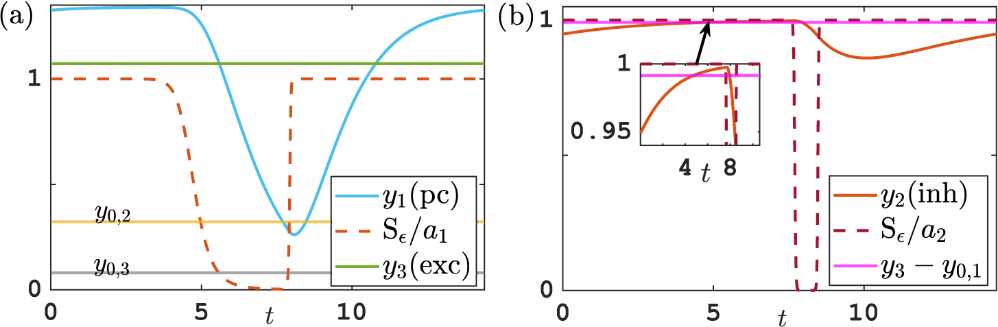
Figure 7 Time profile for alpha-type canard orbit near Hopf bifurcation (labelled HB1, in Figure 4) and activations ${\mathrm {S}}_{\epsilon /a1}$
for
${\mathrm {S}}_{\epsilon /a1}$
for $y_1$
, and
$y_1$
, and ${\mathrm {S}}_{\epsilon /a2}$
for
${\mathrm {S}}_{\epsilon /a2}$
for $y_2$
. Parameters:
$y_2$
. Parameters: $G=1.49\approx G_1=1.48$
(green dashed vertical line in Figure 4 near HB1),
$G=1.49\approx G_1=1.48$
(green dashed vertical line in Figure 4 near HB1), $\epsilon =0.001,y_{0,1},y_{0,3}=0.08$
and
$\epsilon =0.001,y_{0,1},y_{0,3}=0.08$
and $y_{02}=0.3$
, for others, see Table 2. Inset in panel (b) shows that
$y_{02}=0.3$
, for others, see Table 2. Inset in panel (b) shows that $y_2$
crosses the threshold
$y_2$
crosses the threshold $y_{\mathrm {3,eq}}-y_{0,1}$
of
$y_{\mathrm {3,eq}}-y_{0,1}$
of $y_1$
.
$y_1$
.
4.3 Dependence of delta-type oscillations on parameters including nonzero input
Delta-type oscillations in the zero-input case studied here have excitation population potentials $y_1$
and
$y_1$
and $y_3$
at zero until the inhibition
$y_3$
at zero until the inhibition $y_2$
drops sufficiently low such that
$y_2$
drops sufficiently low such that $y_1$
and
$y_1$
and $y_3$
can recover and generate a large-amplitude burst (see Figure 2(e)). The precise time ratios between time spent at zero and bursts depends on time scale ratios such as
$y_3$
can recover and generate a large-amplitude burst (see Figure 2(e)). The precise time ratios between time spent at zero and bursts depends on time scale ratios such as $b^*$
, and thresholds. A positive external input p will affect the time profile and frequency of delta-type oscillations, as positive p will prevent
$b^*$
, and thresholds. A positive external input p will affect the time profile and frequency of delta-type oscillations, as positive p will prevent $y_3$
from staying near zero, resulting in a positive slope at low potential values, as seen in the simulations done by Forrester et al. [Reference Forrester, Crofts, Sotiropoulos, Coombes and O’Dea11] and Ahmadizadeh et al. [Reference Ahmadizadeh, Karoly, Nešić, Grayden, Cook, Soudry and Freestone1].
$y_3$
from staying near zero, resulting in a positive slope at low potential values, as seen in the simulations done by Forrester et al. [Reference Forrester, Crofts, Sotiropoulos, Coombes and O’Dea11] and Ahmadizadeh et al. [Reference Ahmadizadeh, Karoly, Nešić, Grayden, Cook, Soudry and Freestone1].
Acknowledgments
K. Tsaneva-Atanasova gratefully acknowledges the financial support of the Engineering and Physical Sciences Research Council (EPSRC) via grant EP/T017856/1. H. Mahdi gratefully acknowledges the Higher Committee for Education Development (HCED), Government of Iraq, for funding her PhD studies.


 Open access