


1 Introduction
Shimmy, the name of which originally comes from a dance move, is a self-excited lateral and yaw vibration of a wheel assembly, known to be experienced on bicycles, motorcycles, road vehicles and aircraft landing gears. This undesirable vibration typically has a frequency in the range of 10 to 30 Hz and can reach considerable amplitudes, which is potentially dangerous and may result in loss of control or severe damage to mechanical components such as the wheel-suspension system. One of the earliest studies of shimmy was reported by Broulhiet [Reference Broulhiet6] in 1920s, who introduced the concept of side slip which, until now, is still the basis for the understanding of shimmy oscillations in a wide range of wheeled vehicles. Since then, numerous investigations have been conducted and have yielded many positive results to reveal the shimmy mechanism and to provide technical supports for better suppression of shimmy. For details, the literature review by Ran [Reference Ran21], Krüger et al. [Reference Krüger and Morandini15] and Zhang et al. [Reference Zhang36] can act as an entry point to shimmy research.
Shimmy is found to be affected by many factors, such as parameters in the suspension and steering systems [Reference Mi, Stepan, Takacs and Chen18, Reference Wang, Xu, Chen and Meng29], as well as the friction and free-play in the structure [Reference Rahmani and Behdinan20, Reference Zhuravlev, Klimov and Plotnikov37]. Among them, the behaviour of the pneumatic tyre is of particular importance and tyre characteristics, for example, the relaxation length, cornering stiffness and pneumatic trail, are considered as crucial parameters regarding shimmy stability. The milestone for this area was the seminal work of von Schlippe and Dietrich [Reference Schlippe and Dietrich23] on tyre mechanics and its influence on shimmy. The stretched string tyre model they developed formed the basis for almost all tyre models that described tyre transient properties and has been applied extensively in shimmy analysis. Thereafter, the effects of tyre properties, especially the nonlinearities in tyre behaviour, have been of great concern in the field of shimmy analysis. Pacejka [Reference Pacejka19] applied the magic formula to examine the influence of the nonlinear cornering force of the tyre on vehicle shimmy. Research by Ran et al. [Reference Ran, Besselink and Nijmeijer22] highlighted the necessity of a nonlinear tyre model with nonconstant relaxation length in shimmy analysis for more accurate results at large amplitude. Wei et al. [Reference Wei, Li, Xu, Lei and Wang30] discovered that vehicle shimmy could be suppressed by reducing the pneumatic trail, increasing the relaxation length or declining the tyre cornering stiffness related to low-adhesion road. Although these studies have provided strong theoretical references for relevant research, few researchers have addressed the combined influence of different nonlinear tyre characteristics, for example, when they change simultaneously with the tyre inflation pressure, to model more realistic tyre behaviour, especially given Besselink’s work [Reference Besselink, Maas and Nijmeijer4], which showed that the shimmy stability could be very dependent on the tyre model selected and a too simple representation of tyre behaviour could lead to incorrect results.
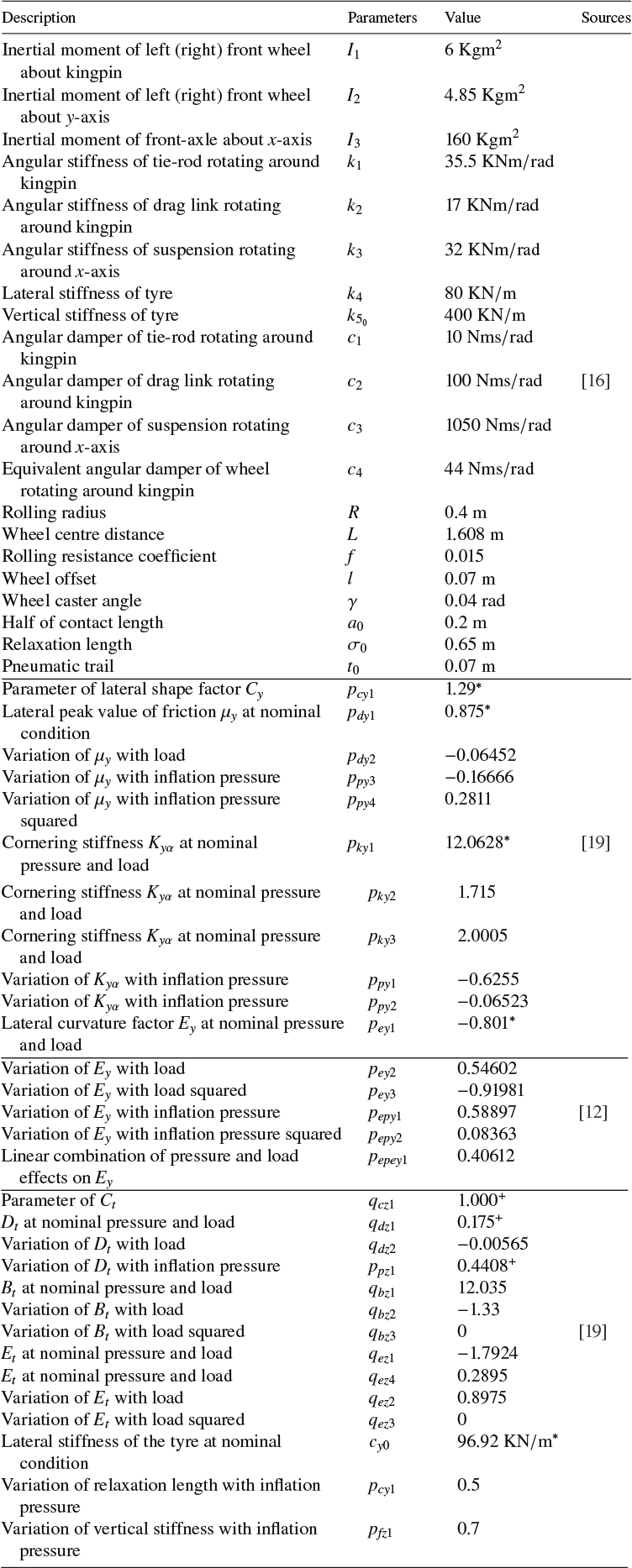
Table 1 Values of parameters with description and data sources.
Tyre inflation pressure plays an important role in vehicle dynamics and handling performance by significantly influencing tyre properties, including lateral, vertical and cornering stiffness and rolling resistance, which has been widely studied by many researchers [Reference Ejsmont, Taryma, Ronowski and Swieczko-Zurek8, Reference Guo, Chen, Xu, Yang and Li10, Reference Wu, Wang and Zhao33]. Most existing research is devoted to extending tyre models, such as the magic formula [Reference Besselink, Schmeitz and Pacejka5, Reference Höpping, Augsburg and Büchner12], the UniTire model [Reference Yang, Xu and Guo34] and others [Reference Höpping, Augsburg and Büchner11, Reference Kasprzak, Lewis and Milliken13], to capture the effects of inflation pressure on different tyre characteristics. For landing gear shimmy, Thota et al. [Reference Thota, Krauskopf, Lowenberg and Coetzee28] modelled six tyre properties as functions of the inflation pressure based on experimental data from two radial tyres to examine how shimmy depended on pressure changes. They found that the area where torsional and lateral shimmy oscillations occurred decreased with an increase in the tyre inflation pressure. For bicycle or motorcycle shimmy, also called wobble, Massaro et al. [Reference Massaro, Cossalter and Cusimano17] experimentally analysed the effect of the inflation pressure on the wobble stability for two types of motorcycle tyres and concluded that despite the difference of wobble stability at high-speeds, increasing pressure was beneficial for low- to medium-speed wobble. In the automotive context, however, the way the inflation pressure affects vehicle shimmy stability has not been well studied. Although the studies reported above can work as academic reference, the different sizes among aviation, motorcycle and vehicle tyres imply the relations they derived may not be representative of automotive applications. More so, since shimmy is a system oscillation and depends both on the tyres as well as the geometry, compliance and inertia of the steering/suspension system.
This work aims not only to study the influence of tyre inflation pressure on shimmy stability but also to consider as many pressure-related tyre properties as possible and to include their nonlinear dependences on inflation pressure in the shimmy model with the purpose of capturing more accurate tyre behaviour. To achieve this, the extended tyre models developed by Besselink [Reference Besselink, Schmeitz and Pacejka5], Pacejka [Reference Pacejka19] and Guo [Reference Guo, Chen, Xu, Yang and Li10] are considered to handle the effect of inflation pressure changes on tyre properties which are found crucial regarding shimmy stability, including tyre lateral force, half-contact length, pneumatic trail, relaxation length and vertical stiffness. Although the lateral stiffness of the tyre and the coefficient of rolling resistance also strongly depend on inflation pressure, their effect on shimmy is limited, which is reflected in bifurcation diagrams as nearly vertical bifurcation curves. Therefore, they are not considered in our research. The extended tyre models are then integrated into the shimmy model established by Li et al. [Reference Li and Lin16] to analyse the influence of inflation pressure on shimmy oscillations, which can clearly demonstrate how the bifurcation curves change when additional nonlinear tyre properties are involved, thereby emphasizing the necessity of considering complex tyre behaviour. One of the contributions of this paper is to reveal the individual and competitive effects of nonlinearities in tyre behaviour on shimmy oscillations with pressure changes.
With regards to analysis methods, time domain simulation is a straightforward, but a less efficient and time-consuming approach, especially when studying the effects of various parameters in a dynamic system. The linearization method, meanwhile, only yields valid conclusions around equilibria and is unable to capture the behaviour of periodic solutions, as well as some critical points like fold bifurcations when the system is unstable. Therefore, the bifurcation analysis based on numerical continuation is used in this work with the aid of the software package COCO. This MATLAB-based platform performs the pseudo-arclength continuation to trace branches of equilibria from an initial equilibrium solution. The Jacobian at each equilibrium point is determined numerically, with stability identified from the eigenvalues of this Jacobian. Bifurcation conditions, such as eigenvalues crossing the imaginary axis, are used to detect and classify bifurcations within equilibria branches. For more information about continuation methods in general, the reader may refer to textbooks on the subject such as [Reference Krauskopf, Osinga and Galán-Vioque14, Reference Strogatz25]; for information about the specific implementation in COCO, the reader may refer to [Reference Ahsan, Dankowicz, Li and Sieber1, Reference Dankowicz and Schilder7]. This method proved to be more effective in determining the boundaries of stable dynamic regimes and the dependency of these regimes on parameters of interest, especially for the model with a high level of nonlinearity. Many substantial studies on shimmy analysis have been carried out using this method. Representative scholars include Stepan and Takacs [Reference Beregi, Takacs and Stepan3, Reference Stépán and Takács24], Thota [Reference Thota, Krauskopf and Lowenberg26, Reference Thota, Krauskopf and Lowenberg27], Ran [Reference Ran21, Reference Ran, Besselink and Nijmeijer22] and Wei [Reference Wei, Lu, Ye and Lu31, Reference Wei, Xu, Wang and Li32].
This paper is organized as follows. Section 2 discusses the mathematical model of steering wheel shimmy of a truck, with the dependency of tyre lateral force on inflation pressure considered in the tyre model. Using this shimmy model, Section 3 presents the effect of forward speed on shimmy for three inflation pressures, providing high-level understanding of the pressure effect. Section 4 is devoted to analysing the influence of the four tyre properties on shimmy oscillations, and then developing the mathematical relations between these tyre properties and inflation pressure. Adding these equations into the model built in Section 2, Section 5 compares the two-parameter bifurcation diagrams of the extended model with the results obtained in Section 3 and demonstrates the importance of considering multiple tyre properties. Section 6 summarizes the results and points to future work. The description, values and sources of all parameters are listed in Table 1, Appendix A.
2 Mathematical model
The shimmy model of a truck with dependent suspension considered in this work is much developed and experimentally validated in a previous work by Li et al. [Reference Li and Lin16]; its schematic view is shown in Figure 1. A global Cartesian coordinate system o-xyz is established such that the x-axis is aligned with the vehicle’s longitudinal axis (driving direction), the z axis is oriented upward normal to x-axis and the y-axis completes the right-handed coordinate system. The model includes three degrees of freedom: two wheels may rotate about the kingpin, giving rise to yaw oscillations described by the yaw angles $\theta _1$
and
$\theta _1$
and $\theta _2$
; the front live axle may also vibrate about the x-axis, resulting in axle tramp described by the tramp angle
$\theta _2$
; the front live axle may also vibrate about the x-axis, resulting in axle tramp described by the tramp angle $\psi $
. They are all marked in red in Figure 1 and oriented about the positive z- and x-axes. The model usually comprises the following three parts: equations of motion, tyre cornering characteristics description and rolling constraint equations for slip angles.
$\psi $
. They are all marked in red in Figure 1 and oriented about the positive z- and x-axes. The model usually comprises the following three parts: equations of motion, tyre cornering characteristics description and rolling constraint equations for slip angles.
A mathematical description of the yaw oscillation and axle tramp is given by the equations of motion:
 $$ \begin{align} I_{1} \ddot{\theta}_{1}&=k_{1}(\theta_{2}-\theta_{1})+c_{1}(\dot{\theta}_{2}-\dot{\theta}_{1})-c_{4} \dot{\theta}_{1}-I_{2} \frac{V}{R} \dot{\psi}\qquad\ \ \kern1pt\qquad\qquad\qquad\qquad\qquad\notag \\ &\quad+\bigg[\frac{L}{2} k_{5} l(\gamma-f)+k_{4} R^{2} \gamma\bigg] \psi-F_{y1}(R \gamma+t), \end{align} $$
 $$ \begin{align} I_{1} \ddot{\theta}_{2}&=k_{1}(\theta_{1}-\theta_{2})+c_{1}(\dot{\theta}_{1}-\dot{\theta}_{2})-(c_{4}+c_{2}) \dot{\theta}_{2}-k_{2} \theta_{2}-I_{2} \frac{V}{R} \dot{\psi}\quad\ \kern1pt\qquad\qquad\qquad\notag \\ &\quad+\bigg[\frac{L}{2} k_{5} l(\gamma-f)+k_{4} R^{2} \gamma\bigg] \psi-F_{y2}(R \gamma+t), \end{align} $$
 $$ \begin{align} I_{3} \ddot{\psi}&=-c_{3} \dot{\psi}-\bigg[k_{3}+\frac{L^{2}}{2} k_{5}+2 k_{4} R^{2}\bigg] \psi+I_{2} \frac{V}{R} \dot{\theta}_{1}+I_{2} \frac{V}{R} \dot{\theta}_{2} +(F_{y1}+F_{y2}) R,\quad \end{align} $$
where R is the rolling wheel radius, L is the wheel centre distance, l is the wheel offset; f is the coefficient of rolling resistance, V is the wheel forward speed and t the pneumatic trail. Here, $\textit {I}_1$
and
$\textit {I}_1$
and $\textit {I}_2$
are the inertia moments of front wheels about the kingpins and y-axis, and
$\textit {I}_2$
are the inertia moments of front wheels about the kingpins and y-axis, and $\textit {I}_3$
the inertia moment of front axle about the x-axis. Linear stiffness and damping terms are used to model the angular compliance of the tie-rod (
$\textit {I}_3$
the inertia moment of front axle about the x-axis. Linear stiffness and damping terms are used to model the angular compliance of the tie-rod ( $\textit {k}_1,\textit {c}_1$
), the drag link (
$\textit {k}_1,\textit {c}_1$
), the drag link ( $\textit {k}_2,\textit {c}_2$
) and the suspension (
$\textit {k}_2,\textit {c}_2$
) and the suspension ( $\textit {k}_3,\textit {c}_3$
), as shown in Figure 1. Furthermore,
$\textit {k}_3,\textit {c}_3$
), as shown in Figure 1. Furthermore, $\textit {k}_4$
and
$\textit {k}_4$
and $\textit {k}_5$
represent the lateral and vertical stiffness of the tyre, respectively, and
$\textit {k}_5$
represent the lateral and vertical stiffness of the tyre, respectively, and $\textit {c}_4$
is the angular damping of wheels rotating around the kingpins. In addition, note that the linearization of sine functions is adopted due to the small values of the caster angle
$\textit {c}_4$
is the angular damping of wheels rotating around the kingpins. In addition, note that the linearization of sine functions is adopted due to the small values of the caster angle $\gamma $
and the tramp angle
$\gamma $
and the tramp angle $\psi $
. The lateral force
$\psi $
. The lateral force $F_{y1}$
and
$F_{y1}$
and $F_{y2}$
are determined by a tyre model, which is explained in detail in the following section.
$F_{y2}$
are determined by a tyre model, which is explained in detail in the following section.
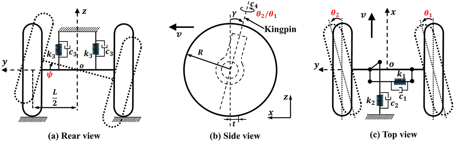
Figure 1 Model of steering wheel shimmy for (a) rear view, (b) side view and (c) top view.
2.1 Tyre lateral characteristics
Precise expression for cornering characteristics of the tyre is crucial for effective analysis of steering wheel shimmy. The magic formula is a widely used semi-empirical tyre model to describe the nonlinearity of tyre lateral force. The lateral force equations are as follows:
 $$ \begin{align} F_{y1}&=-D_{y} \sin \{C_{y} \arctan [B_{y} \alpha_{1}-E_{y}(B_{y} \alpha_{1}-\arctan (B_{y} \alpha_{1}))]\}, \end{align} $$
 $$ \begin{align} F_{y2}&=-D_{y} \sin \{C_{y} \arctan [B_{y} \alpha_{2}-E_{y}(B_{y} \alpha_{2}-\arctan (B_{y} \alpha_{2}))]\}, \end{align} $$
where $\alpha _1$
and
$\alpha _1$
and $\alpha _2$
represent the slip angles of right and left tyres, and both are oriented about the positive z-axis;
$\alpha _2$
represent the slip angles of right and left tyres, and both are oriented about the positive z-axis; $\textit {B}_y$
,
$\textit {B}_y$
, $\textit {C}_y$
,
$\textit {C}_y$
, $\textit {D}_y$
,
$\textit {D}_y$
, $\textit {E}_y$
are four factors that can adjust the shape of force curve. In this work, these parameters are modelled as functions of tyre inflation pressure according to the extended formulations by Pacejka [Reference Pacejka19], to handle pressure changes. In addition, it is noteworthy that the curvature factor
$\textit {E}_y$
are four factors that can adjust the shape of force curve. In this work, these parameters are modelled as functions of tyre inflation pressure according to the extended formulations by Pacejka [Reference Pacejka19], to handle pressure changes. In addition, it is noteworthy that the curvature factor $\textit {E}_y$
is found to be negatively related to the inflation pressure [Reference Guo, Chen, Xu, Yang and Li10], whilst the extended expression of
$\textit {E}_y$
is found to be negatively related to the inflation pressure [Reference Guo, Chen, Xu, Yang and Li10], whilst the extended expression of $\textit {E}_y$
by Pacejka [Reference Pacejka19] does not include this influence. As a result, with reference to Hopping’s work [Reference Höpping, Augsburg and Büchner12], improvement is made based on this with second-order polynomials applied to describe the empirical relationship between
$\textit {E}_y$
by Pacejka [Reference Pacejka19] does not include this influence. As a result, with reference to Hopping’s work [Reference Höpping, Augsburg and Büchner12], improvement is made based on this with second-order polynomials applied to describe the empirical relationship between $\textit {E}_y$
and inflation pressure. The detailed expressions of these factors are introduced as follows:
$\textit {E}_y$
and inflation pressure. The detailed expressions of these factors are introduced as follows:
 $$ \begin{align} C_{y}&=p_{cy1},\quad\qquad\qquad\qquad\qquad\qquad\qquad\qquad\qquad\qquad\qquad\qquad \end{align} $$
 $$ \begin{align} \kern-2.5pt D_{y}&=\mu_{y} F_{z}=F_{z}(p_{dy1}+p_{dy2} \,df_{z})(1+p_{py3} \,dp_{i}+p_{py4} \,{dp_{i}}^{2}),\qquad\qquad\quad \end{align} $$
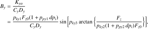 $$ \begin{align} B_{y}&=\frac{K_{y \alpha}}{C_{y} D_{y}}\quad\notag \\ &=\frac{p_{ky1} F_{z0}(1+p_{py1} \,d p_{i})}{C_{y} D_{y}} \sin \bigg[p_{ky3} \arctan \bigg\{\frac{F_{z}}{p_{ky2}(1+p_{py2} \,dp_{i}) F_{z0}}\bigg\}\bigg],\quad \end{align} $$
 $$ \begin{align} \kern-1pt E_{y}&=p_{ey1}+p_{ey2} \,d f_{z}+p_{ey3} \,{df_{z}}^{2}+p_{epy1} \,dp_{i}+p_{epy2} \,{dp_{i}}^{2}+p_{epey1} \,df_{z} \,dp_{i}, \end{align} $$
where $\mu _y$
is the peak lateral friction coefficient and
$\mu _y$
is the peak lateral friction coefficient and $K_{y\alpha }$
the cornering stiffness;
$K_{y\alpha }$
the cornering stiffness; ${dp}_i$
,
${dp}_i$
, ${df}_z$
are the changes in tyre inflation pressure and vertical load, which are given by
${df}_z$
are the changes in tyre inflation pressure and vertical load, which are given by
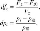 $$ \begin{align*} df_{z}&=\frac{F_z-F_{z0}}{F_z},\\ dp_{i}&=\frac{p_i-p_{i0}}{p_{i0}}. \end{align*} $$
Here, $p_i$
,
$p_i$
, $F_z$
describe the actual inflation pressure and vertical load;
$F_z$
describe the actual inflation pressure and vertical load; $p_{i0}$
and
$p_{i0}$
and $F_{z0}$
represent the nominal pressure and vertical load, which are assumed to be 2.5 bar and 6000 N in this work. In addition,
$F_{z0}$
represent the nominal pressure and vertical load, which are assumed to be 2.5 bar and 6000 N in this work. In addition, $F_z$
remains unchanged at
$F_z$
remains unchanged at $F_{z0}$
in the following bifurcation analysis so that the influence of pressure changes can be highlighted. Other coefficients in (2.6)–(2.9) are described in Appendix A. The coefficient values of
$F_{z0}$
in the following bifurcation analysis so that the influence of pressure changes can be highlighted. Other coefficients in (2.6)–(2.9) are described in Appendix A. The coefficient values of $C_y$
,
$C_y$
, $\mu _y$
and
$\mu _y$
and $K_{y\alpha }$
come from an example tyre in Pacejka’s work [Reference Pacejka19] (205/60R15 91 V), and the coefficients in
$K_{y\alpha }$
come from an example tyre in Pacejka’s work [Reference Pacejka19] (205/60R15 91 V), and the coefficients in $E_y$
refer to [Reference Höpping, Augsburg and Büchner12] to capture the similar trend of the curve’s curvature with inflation pressure. Figure 2 illustrates how the lateral force varies with the slip angle for different pressures, showing the significant dependency of force curves on inflation pressure. However, during transient motion like shimmy oscillations, the tyre’s slip angle has some important dynamics associated with it, and these also strongly depend on its inflation pressure. The tyre model, therefore, needs to account for the constraint equations for slip angle to accurately capture related behaviours, which is presented in the next section.
$E_y$
refer to [Reference Höpping, Augsburg and Büchner12] to capture the similar trend of the curve’s curvature with inflation pressure. Figure 2 illustrates how the lateral force varies with the slip angle for different pressures, showing the significant dependency of force curves on inflation pressure. However, during transient motion like shimmy oscillations, the tyre’s slip angle has some important dynamics associated with it, and these also strongly depend on its inflation pressure. The tyre model, therefore, needs to account for the constraint equations for slip angle to accurately capture related behaviours, which is presented in the next section.
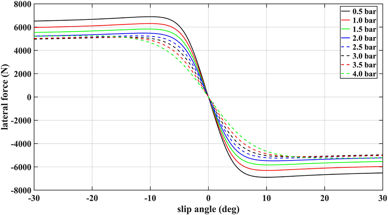
Figure 2 Influence of inflation pressure on the curve of lateral force.
2.2 Rolling constraint equations for slip angle
During transient motion, the mechanics of a rolling tyre, such as the lateral deflection, is described by the stretched string model with a finite contact length [Reference Schlippe and Dietrich23]. In this model, for points in the contact region, the assumption is made that no sliding occurs with respect to the road. Additionally, since from its approximation, tyres cannot respond instantaneously, the influence of the tyre relaxation length $\sigma $
is revealed in the kinematics. The non-holonomic rolling constraint equations that govern the tyre’s slip angle are expressed as
$\sigma $
is revealed in the kinematics. The non-holonomic rolling constraint equations that govern the tyre’s slip angle are expressed as
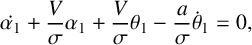 $$ \begin{align} \dot{\alpha_1}+\frac{V}{\sigma} \alpha_1+\frac{V}{\sigma} \theta_1-\frac{a}{\sigma} \dot{\theta}_1=0, \end{align} $$
 $$ \begin{align} \dot{\alpha_2}+\frac{V}{\sigma} \alpha_2+\frac{V}{\sigma} \theta_2-\frac{a}{\sigma} \dot{\theta_2}=0, \end{align} $$
where a is the half-length of the tyre contact patch.
Finally, substitution of the tyre lateral force equations (2.4)–(2.5) into the equations of motion (2.1)–(2.3), coupled with the constraint equations (2.10) and (2.11), completes the shimmy model of steering wheels, which can be expressed in the form of a state matrix with respect to bifurcation parameters:
 $$ \begin{align} \dot{x}=f(p, x), \end{align} $$
where $x=(\theta _1,\dot {\theta _1},\theta _2,\dot {\theta _2},\psi ,\dot {\psi },\alpha _1,\alpha _2 )^T$
represents the system state variable and
$x=(\theta _1,\dot {\theta _1},\theta _2,\dot {\theta _2},\psi ,\dot {\psi },\alpha _1,\alpha _2 )^T$
represents the system state variable and ${p=(p_i,V)^T}$
is the bifurcation parameter. In terms of the four pressure-dependent tyre properties a, t,
${p=(p_i,V)^T}$
is the bifurcation parameter. In terms of the four pressure-dependent tyre properties a, t, $\sigma $
and
$\sigma $
and $k_5$
, in Section 3, they are fixed at initial values which are obtained from the literature [Reference Li and Lin16] and marked as
$k_5$
, in Section 3, they are fixed at initial values which are obtained from the literature [Reference Li and Lin16] and marked as $a_0$
,
$a_0$
, $t_0$
,
$t_0$
, $\sigma _0$
and
$\sigma _0$
and $k_{5_0}$
in Appendix A. In Section 4, however, these four tyre characteristics are also regarded as bifurcation parameters to investigate their effects. Unless otherwise specified, when one property is changed, the other three remain at their initial values. The values of other parameters in the model are given in Appendix A.
$k_{5_0}$
in Appendix A. In Section 4, however, these four tyre characteristics are also regarded as bifurcation parameters to investigate their effects. Unless otherwise specified, when one property is changed, the other three remain at their initial values. The values of other parameters in the model are given in Appendix A.
3 The effect of inflation pressure on shimmy
In this section, a bifurcation analysis on the created model (2.12) is carried out to indicate the wheel’s nonlinear dynamics response and the onset of shimmy oscillations. The bifurcation diagrams for the forward speed V against the yaw angle of the right wheel $\theta _1$
and the tramp angle
$\theta _1$
and the tramp angle $\psi $
at nominal pressure
$\psi $
at nominal pressure $p_{i0}$
(2.5 bar) are first presented in Figure 3 as the baseline case with graphical conventions defined in the legend. Due to the symmetry of the system considered, the configuration of zero yaw angle and zero tramp angle is always an equilibrium. Therefore, a stable band of equilibria is located at the zero position as the speed V is increased from 0, where the system is stable and free of shimmy. Changes in its stability occur when Hopf bifurcations emerge, which gives rise to periodic orbits, that is, shimmy oscillations. Since these limit cycles are all symmetric with respect to the zero position, only the parts above zero are shown in this work. As shown in Figure 3, a supercritical Hopf bifurcation HB1 occurs when V reaches 46.14 km/h, leading to a stable limit cycle, where the wheels oscillate around the kingpin and the axle tramps around the x-axis at an amplitude which increases as V goes up; when V reaches 56.34 km/h, the amplitude of
$p_{i0}$
(2.5 bar) are first presented in Figure 3 as the baseline case with graphical conventions defined in the legend. Due to the symmetry of the system considered, the configuration of zero yaw angle and zero tramp angle is always an equilibrium. Therefore, a stable band of equilibria is located at the zero position as the speed V is increased from 0, where the system is stable and free of shimmy. Changes in its stability occur when Hopf bifurcations emerge, which gives rise to periodic orbits, that is, shimmy oscillations. Since these limit cycles are all symmetric with respect to the zero position, only the parts above zero are shown in this work. As shown in Figure 3, a supercritical Hopf bifurcation HB1 occurs when V reaches 46.14 km/h, leading to a stable limit cycle, where the wheels oscillate around the kingpin and the axle tramps around the x-axis at an amplitude which increases as V goes up; when V reaches 56.34 km/h, the amplitude of $\theta _1$
and
$\theta _1$
and $\psi $
peaks at
$\psi $
peaks at $3.45^{\circ }$
and
$3.45^{\circ }$
and $0.14^{\circ }$
, respectively, and starts to decrease; the stable oscillations end at another supercritical Hopf bifurcation HB2 (70.5 km/h). The results calculated by numerical continuation match those obtained by Li et al. [Reference Li and Lin16, Figure 8], a model which has been verified by road experiments.
$0.14^{\circ }$
, respectively, and starts to decrease; the stable oscillations end at another supercritical Hopf bifurcation HB2 (70.5 km/h). The results calculated by numerical continuation match those obtained by Li et al. [Reference Li and Lin16, Figure 8], a model which has been verified by road experiments.
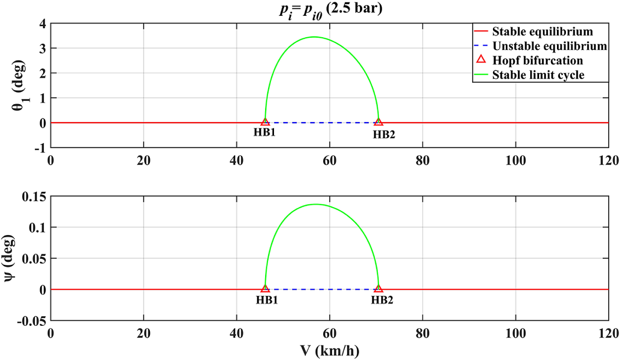
Figure 3 One-parameter bifurcation diagrams at nominal inflation pressure.

Figure 4 One-parameter bifurcation diagrams for inflation pressures (a) 1.5 bar and (b) 2.7 bar.
As the inflation pressure $p_i$
is decreased to
$p_i$
is decreased to $0.6p_{i0}$
(1.5 bar), however, the continuation results are changed significantly, as presented in Figure 4(a) with the same graphical conventions as Figure 3. Several important features can be noted after comparison: the speed range of the limit cycle bounded by HB1 (27.63 km/h) and HB2 (97.13 km/h) expands nearly three times and the same goes for the peak amplitude of
$0.6p_{i0}$
(1.5 bar), however, the continuation results are changed significantly, as presented in Figure 4(a) with the same graphical conventions as Figure 3. Several important features can be noted after comparison: the speed range of the limit cycle bounded by HB1 (27.63 km/h) and HB2 (97.13 km/h) expands nearly three times and the same goes for the peak amplitude of $\theta _1$
(
$\theta _1$
( $9.85^{\circ }$
) and
$9.85^{\circ }$
) and $\psi $
(
$\psi $
( $0.41^{\circ }$
); new supercritical Hopf bifurcations HB3 and HB4 appear at 192.98 and 345.89 km/h, respectively, giving rise to a new stable limit cycle with the maximum amplitude of
$0.41^{\circ }$
); new supercritical Hopf bifurcations HB3 and HB4 appear at 192.98 and 345.89 km/h, respectively, giving rise to a new stable limit cycle with the maximum amplitude of $3.18^{\circ }$
for
$3.18^{\circ }$
for $\theta _1$
and
$\theta _1$
and $0.92^{\circ }$
for
$0.92^{\circ }$
for $\psi $
. This is the emergence of the second shimmy mode. Additionally, the frequency of the second mode (10.6–13.2 Hz) is always higher than the first mode (5.28–6.66 Hz). Since for the yaw motion, the amplitude of the first mode is larger, but for the tramp motion, the larger amplitude emerges in the second mode, the first mode hereinafter is called the yaw mode and the second the tramp mode. It can be seen from the comparison between Figures 3 and 4(a) that the system exhibits more unstable behaviour at low inflation pressures and shimmy occurs over a wider range of speeds. In contrast, with regards to high pressures (2.7 bar), the two modes both vanish and the stable bands of equilibria cross the diagrams (Figure 4(b)) from left to right, meaning that shimmy disappears and that the system remains stable at any speed.
$\psi $
. This is the emergence of the second shimmy mode. Additionally, the frequency of the second mode (10.6–13.2 Hz) is always higher than the first mode (5.28–6.66 Hz). Since for the yaw motion, the amplitude of the first mode is larger, but for the tramp motion, the larger amplitude emerges in the second mode, the first mode hereinafter is called the yaw mode and the second the tramp mode. It can be seen from the comparison between Figures 3 and 4(a) that the system exhibits more unstable behaviour at low inflation pressures and shimmy occurs over a wider range of speeds. In contrast, with regards to high pressures (2.7 bar), the two modes both vanish and the stable bands of equilibria cross the diagrams (Figure 4(b)) from left to right, meaning that shimmy disappears and that the system remains stable at any speed.
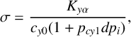
Figure 4 clearly illustrates that the inflation pressure has a qualitative influence on the bifurcations observed over a range of speeds, and thereby on shimmy oscillations. To provide a global picture of how $p_i$
affects shimmy oscillations, a two-parameter continuation is performed in the (V,
$p_i$
affects shimmy oscillations, a two-parameter continuation is performed in the (V, $p_i$
) plane, as shown in Figure 5. The curves of HB1–HB4 changing with pressure divide the plane into regions corresponding to different behaviour of the system. In the region in shadow, there is no shimmy oscillations, that is, the straight-rolling motion is stable, but the system becomes unstable and experiences shimmy oscillations in the white region, including the yaw mode and the tramp mode. It can be seen from the bifurcation diagram that there is a same trend in the two modes with inflation pressure changes. Increasing
$p_i$
) plane, as shown in Figure 5. The curves of HB1–HB4 changing with pressure divide the plane into regions corresponding to different behaviour of the system. In the region in shadow, there is no shimmy oscillations, that is, the straight-rolling motion is stable, but the system becomes unstable and experiences shimmy oscillations in the white region, including the yaw mode and the tramp mode. It can be seen from the bifurcation diagram that there is a same trend in the two modes with inflation pressure changes. Increasing $p_i$
significantly suppresses and eventually eliminates shimmy oscillations: the speed ranges of the two modes are reduced to zero at (252 km/h, 1.73 bar (
$p_i$
significantly suppresses and eventually eliminates shimmy oscillations: the speed ranges of the two modes are reduced to zero at (252 km/h, 1.73 bar ( $0.69p_{i0}$
)) and at fold bifurcation F1 (57.79 km/h, 2.61 bar (
$0.69p_{i0}$
)) and at fold bifurcation F1 (57.79 km/h, 2.61 bar ( $1.044p_{i0}$
)), whilst decreasing
$1.044p_{i0}$
)), whilst decreasing $p_i$
leads to the opposite tendency. These results qualitatively agree with the work on landing gear shimmy by Thota et al. [Reference Thota, Krauskopf, Lowenberg and Coetzee28] and on motorcycle shimmy by Massaro et al. [Reference Massaro, Cossalter and Cusimano17]. In comparison, with the reduction of
$p_i$
leads to the opposite tendency. These results qualitatively agree with the work on landing gear shimmy by Thota et al. [Reference Thota, Krauskopf, Lowenberg and Coetzee28] and on motorcycle shimmy by Massaro et al. [Reference Massaro, Cossalter and Cusimano17]. In comparison, with the reduction of $p_i$
, the tramp mode expands much faster than the yaw mode: the curve of HB4 exceeds the boundary of the diagram rapidly after 1 bar. It is also worth mentioning that there is no interaction between the two modes even when the pressure is close to zero. In other words, the stable region between the two modes always exists. Despite the qualitative agreement with previous work, the influence of inflation pressure on the tyre model is incomplete as only tyre lateral force was considered. The following section explores how other tyre properties, which are known to heavily depend on pressure, significantly influence these shimmy oscillations.
$p_i$
, the tramp mode expands much faster than the yaw mode: the curve of HB4 exceeds the boundary of the diagram rapidly after 1 bar. It is also worth mentioning that there is no interaction between the two modes even when the pressure is close to zero. In other words, the stable region between the two modes always exists. Despite the qualitative agreement with previous work, the influence of inflation pressure on the tyre model is incomplete as only tyre lateral force was considered. The following section explores how other tyre properties, which are known to heavily depend on pressure, significantly influence these shimmy oscillations.
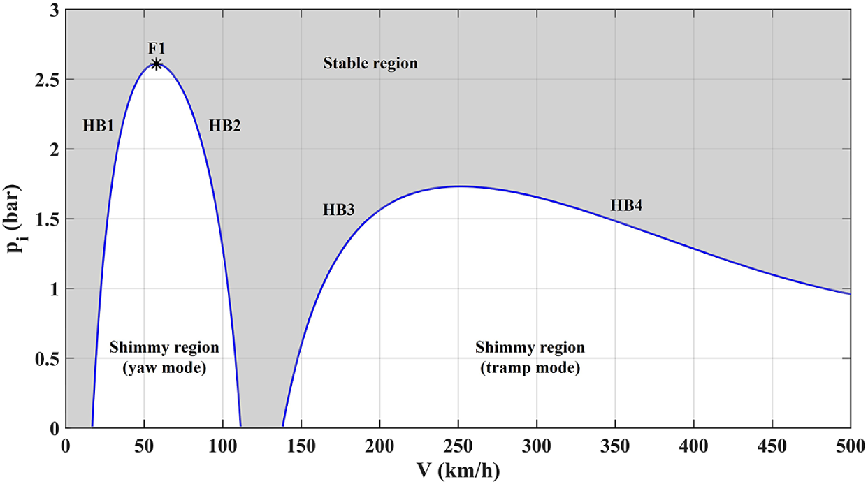
Figure 5 Effect of tyre inflation pressure on the Hopf bifurcations with lateral force changes considered.
4 Effect of pressure-dependent tyre properties on shimmy
As the aim of our paper is to study the nonlinear dynamics that can arise within the equations of motion for the shimmy phenomenon, this section first illustrates how each of the four pressure-dependent tyre properties independently influence the shimmy response when changed relative to the others, before combining their effects as a function of inflation pressure. Presenting these relative changes provides insight into the range of responses that could be obtained from this shimmy model, highlighting competing mechanisms whose relative magnitudes will change from tyre to tyre. Two-parameter bifurcation diagrams are obtained to demonstrate the two shimmy modes as functions of these properties for different inflation pressures. As with Figure 5, the stable regions for all pressures are shaded to separately identify different domains. The mathematical dependency of these properties on inflation pressure is then modelled to be incorporated into the shimmy model in the next section. To provide a complete view of the overall dynamics, the range of tyre characteristic values in the following analysis is much greater than general operation values.
4.1 Half-contact length
In the modelling of the motion stability, controllability and braking dynamics of vehicles, information about the tyre’s half-contact length with the road surface is crucial [Reference Balakina, Zadvornov, Sarbaev, Sergienko and Kozlov2]. The half-contact length a is a geometrical property and directly dependent on vertical tyre deflection, which is heavily influenced by tyre inflation pressure $p_i$
. Typically, a decrease in
$p_i$
. Typically, a decrease in $p_i$
results in increased vertical deflection, thereby larger contact length. The change in a can affect shimmy substantially for different inflation pressures, which can be observed in Figure 6. At
$p_i$
results in increased vertical deflection, thereby larger contact length. The change in a can affect shimmy substantially for different inflation pressures, which can be observed in Figure 6. At $p_{i0}$
(2.5 bar), for example, as a is slightly reduced from 0.2 m to 0.186 m, HB1 and HB2 which bound the yaw mode quickly approach each other and eventually collide, indicating the disappearance of shimmy. However, when there are two modes at 0.6
$p_{i0}$
(2.5 bar), for example, as a is slightly reduced from 0.2 m to 0.186 m, HB1 and HB2 which bound the yaw mode quickly approach each other and eventually collide, indicating the disappearance of shimmy. However, when there are two modes at 0.6 $p_{i0}$
(1.5 bar), a only has a quantitative effect on the tramp mode (its speed range is decreased with the reduction of a). In addition, with the increase in
$p_{i0}$
(1.5 bar), a only has a quantitative effect on the tramp mode (its speed range is decreased with the reduction of a). In addition, with the increase in $p_i$
from 0.6
$p_i$
from 0.6 $p_{i0}$
to 1.2
$p_{i0}$
to 1.2 $p_{i0}$
(3 bar), the area where the yaw mode occurs gradually shrinks and the intersection points of HB1 and HB2 curves continue to move upward almost vertically, which means that the speed at which bifurcations intersect remain unchanged (58 km/h), but the value of a that makes shimmy appear is getting increasingly higher. Since a is decreased with increasing pressure, this will obviously speed up the disappearance of shimmy.
$p_{i0}$
(3 bar), the area where the yaw mode occurs gradually shrinks and the intersection points of HB1 and HB2 curves continue to move upward almost vertically, which means that the speed at which bifurcations intersect remain unchanged (58 km/h), but the value of a that makes shimmy appear is getting increasingly higher. Since a is decreased with increasing pressure, this will obviously speed up the disappearance of shimmy.

Figure 6 Effect of half-contact length on the Hopf bifurcations for four inflation pressures.
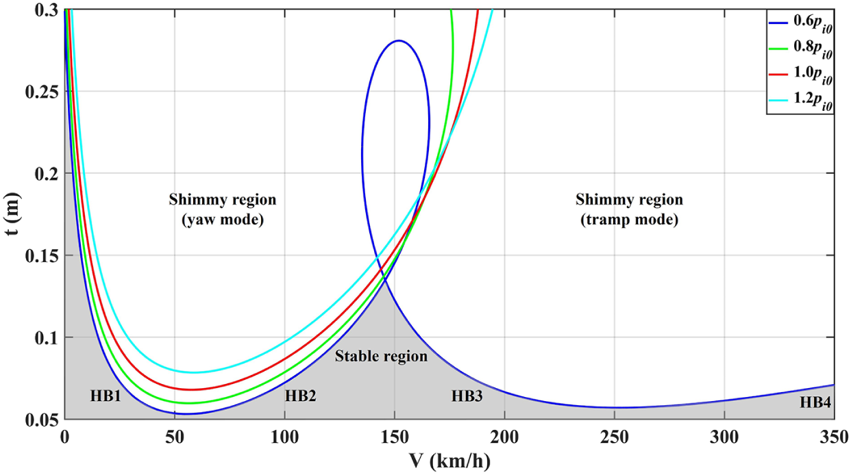
Figure 7 Effect of pneumatic trail on the Hopf bifurcations for four inflation pressures.
In this work, according to Guo’s experiment [Reference Guo, Chen, Xu, Yang and Li10], the half-contact length is defined to be proportional with the square root of the wheel load and the tyre inflation pressure:
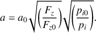 $$ \begin{align} a = a_0 \sqrt{\bigg( \frac{F_z}{F_{z0}} \bigg)} \sqrt{\Bigg( \frac{p_{i0}}{p_i} \Bigg)}. \end{align} $$
4.2 Pneumatic trail
Pneumatic trail t is the distance along the x-axis between the centre of contact patch and the point where the lateral force is applied, which determines the moment arm of the lateral force related to the generation of the self-aligning moment. Its effect on shimmy (Figure 7) illustrates that in terms of the yaw model, the intersection points of HB1 and HB2 have a similar trend to those in Figure 6, while the upward movement is much slower with increasing $p_i$
. In addition, when t = 0.1 m, the region where the yaw mode occurs shrinks for high pressures, but this tendency reverses when t exceeds a certain value (approximately 0.2 m). For instance, at 0.25 m, the range of the yaw mode expands as
$p_i$
. In addition, when t = 0.1 m, the region where the yaw mode occurs shrinks for high pressures, but this tendency reverses when t exceeds a certain value (approximately 0.2 m). For instance, at 0.25 m, the range of the yaw mode expands as $p_i$
is increased. This reversal is closely related to the onset of the tramp mode at low pressures and when it comes to the tramp mode, the effect of t is more complicated than that of a. At 0.6
$p_i$
is increased. This reversal is closely related to the onset of the tramp mode at low pressures and when it comes to the tramp mode, the effect of t is more complicated than that of a. At 0.6 $p_{i0}$
, for example, t can cause qualitative changes in both modes. The details are shown in Figure 8. With a reduction of t from 0.07 to 0.05 m, HB1 and HB2 approach each other and merge, and the same goes for HB3 and HB4, leading to the disappearance of the two modes at similar t values (0.053 m and 0.057 m). When t grows, the main feature is the closed loop formed by HB2 of the yaw mode and HB3 of the tramp mode after their intersection in the Hopf–Hopf bifurcation HH (
$p_{i0}$
, for example, t can cause qualitative changes in both modes. The details are shown in Figure 8. With a reduction of t from 0.07 to 0.05 m, HB1 and HB2 approach each other and merge, and the same goes for HB3 and HB4, leading to the disappearance of the two modes at similar t values (0.053 m and 0.057 m). When t grows, the main feature is the closed loop formed by HB2 of the yaw mode and HB3 of the tramp mode after their intersection in the Hopf–Hopf bifurcation HH ( $t=0.135$
m). The two modes overlap after this codimension-two point and finally merge into one mode when
$t=0.135$
m). The two modes overlap after this codimension-two point and finally merge into one mode when $t>0.28$
m. Specifically, in this loop, two torus bifurcation curves T1 (in the yaw mode) and T2 (in the tramp mode) are found to emerge locally after HH, which agrees with what may be expected from bifurcation theory. In addition, the criticality of HB2 and HB3 changes from supercritical to subcritical Hopf bifurcation at two degenerate Hopf bifurcation points DH1 (0.146 m) and DH2 (0.216 m), giving birth to unstable shimmy oscillations. This verifies Li’s inference in their work [Reference Li and Lin16] that some unstable limit cycles can occur if other nonlinear factors are properly considered in the model. Two curves of saddle-node bifurcation S1 (in the yaw mode) and S2 (in the tramp mode) appear from DH1 and DH2 successively.
$t>0.28$
m. Specifically, in this loop, two torus bifurcation curves T1 (in the yaw mode) and T2 (in the tramp mode) are found to emerge locally after HH, which agrees with what may be expected from bifurcation theory. In addition, the criticality of HB2 and HB3 changes from supercritical to subcritical Hopf bifurcation at two degenerate Hopf bifurcation points DH1 (0.146 m) and DH2 (0.216 m), giving birth to unstable shimmy oscillations. This verifies Li’s inference in their work [Reference Li and Lin16] that some unstable limit cycles can occur if other nonlinear factors are properly considered in the model. Two curves of saddle-node bifurcation S1 (in the yaw mode) and S2 (in the tramp mode) appear from DH1 and DH2 successively.
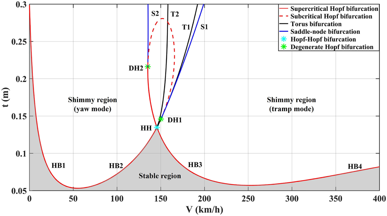
Figure 8 Effect of pneumatic trail on the Hopf bifurcations at 0.6 $p_{i0}$
.
$p_{i0}$
.
To understand how shimmy oscillations are changed with t after the closed loop and new bifurcations are detected, the limit cycles at two pneumatic trails are presented in Figure 9. In panel (a), for the yaw mode, the bifurcating shimmy oscillations remain stable up to S1 (184.75 km/h). Here, the branch turns back, and, after the immediate T1 (181.65 km/h), it connects to the zero-equilibrium, which does not regain stability because of the overlap of the two modes. Therefore, when S1 is crossed, a jump phenomenon happens: shimmy suddenly changes from the yaw mode to the tramp mode, alongside a significant increase in amplitude, as demonstrated in Figure 10(a). In contrast, for the tramp mode, the oscillations are initially unstable due to the subcritical Hopf bifurcation HB3 and then become stable after T2 (157.39 km/h), which is preceded by S2 (135.56 km/h). Thus, if V is reduced past T2, the shimmy oscillations experience a similar sudden change to the stable yaw mode from the unstable tramp mode, which is shown as the significantly reduced amplitude in Figure 10(b). It should also be noted that the region between T2 and S1 indicates bi-stability, where the stable yaw and tramp modes coexist. In this region, which steady-state solution can be observed depends on initial conditions. The phase portrait in the plane of $\psi $
and
$\psi $
and $\dot {\psi }$
at 180 km/h (Figure 11) can provide greater insight into this dependency. Two initial conditions L1 and L2 shown as solid squares lead to completely different simulation trajectories, one of which converges to the stable tramp mode (the grey curve from L1), while the other is attracted by the stable yaw mode (the black curve from L2).
$\dot {\psi }$
at 180 km/h (Figure 11) can provide greater insight into this dependency. Two initial conditions L1 and L2 shown as solid squares lead to completely different simulation trajectories, one of which converges to the stable tramp mode (the grey curve from L1), while the other is attracted by the stable yaw mode (the black curve from L2).
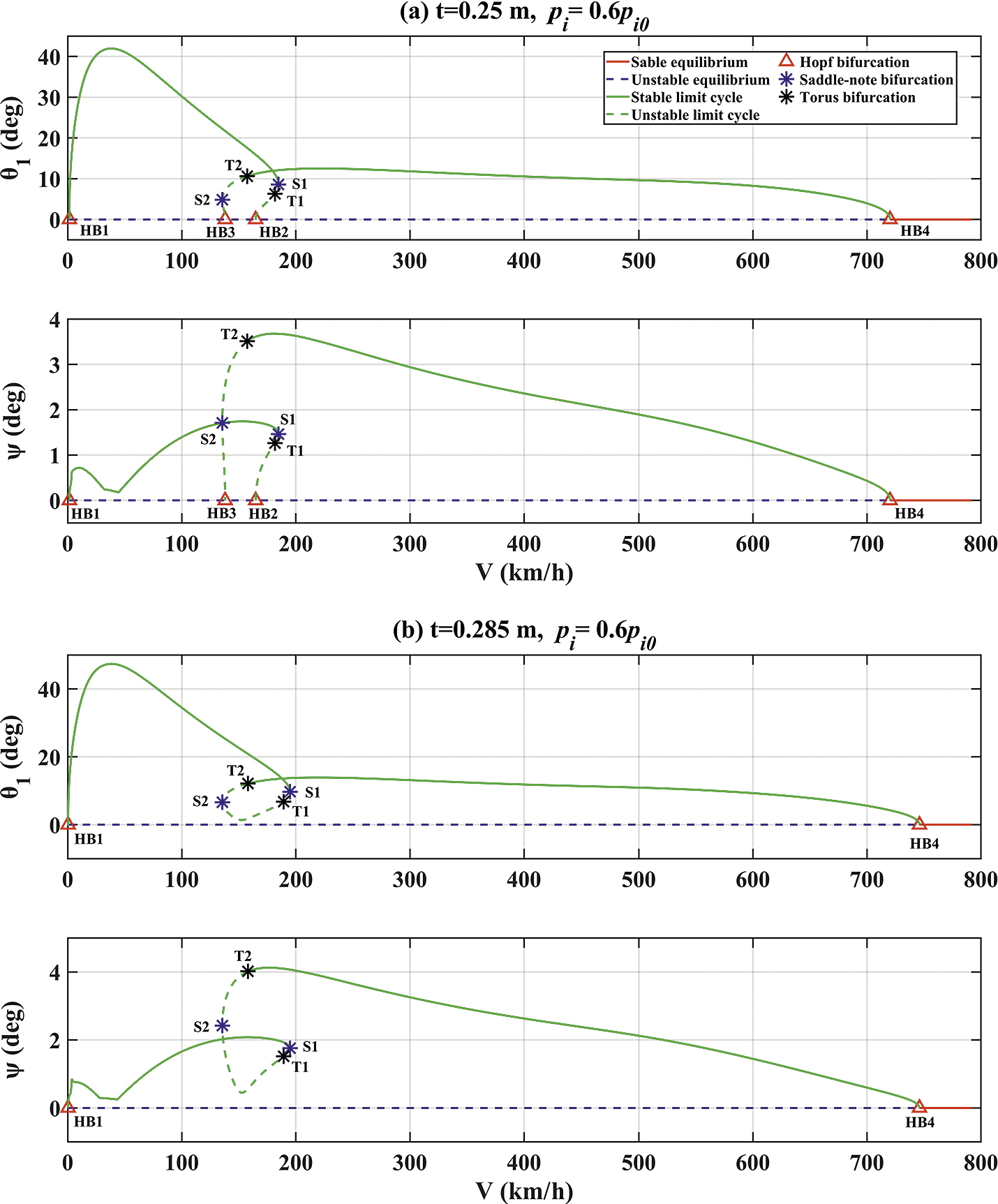
Figure 9 One-parameter bifurcation diagram for pneumatic trail (a) 0.25 m and (b) 0.285 m at the same inflation pressure.

Figure 10 Time-history simulations of mode changes at 0.25 m and 1.5 bar with (a) increasing speed and (b) decreasing speed.
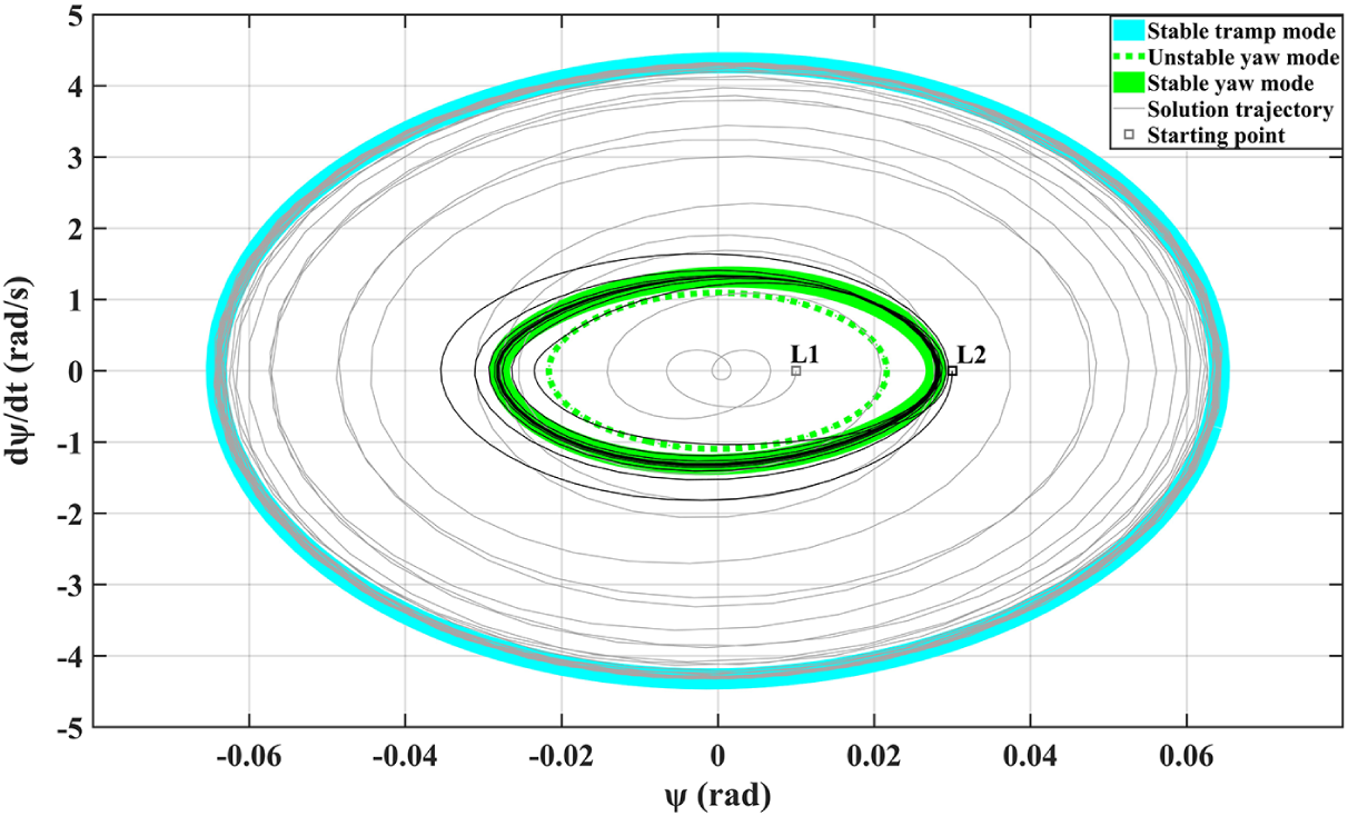
Figure 11 Phase portrait of bi-stable region at 180 km/h.
When t rises to 0.285 m (Figure 9(b)), HB2 and HB3 collide and disappear, making the unstable periodic orbits between S1 and T2 connected, and the two modes become one mode bounded by the supercritical Hopf bifurcations HB1 and HB4, with a large range of speeds covered. As a result, compared with Figure 4(a), the area where shimmy happens in Figure 9 expands dramatically and the peak amplitude is increased nearly fourfold with a growth of t.
Literature [Reference Gipser9, Reference Yang, Xu and Guo34] has indicated that pneumatic trail decreases with an increase in tyre inflation pressure and slip angle. Their relationships are obtained from the extended magic formula, with similar equations to tyre force:
 $$ \begin{align} t_1&=D_t \cos \{C_t \arctan [B_t \alpha_1-E_{t1}(B_t \alpha_1-\arctan (B_t \alpha_1))]\}, \end{align} $$
 $$ \begin{align} t_2&=D_t \cos \{C_t \arctan [B_t \alpha_2-E_{t2}(B_t \alpha_2-\arctan (B_t \alpha_2))]\}, \end{align} $$
where, similarly, $B_t$
,
$B_t$
, $C_t$
,
$C_t$
, $D_t$
,
$D_t$
, $E_t$
are four factors that can adjust the shape of curves. They are given by
$E_t$
are four factors that can adjust the shape of curves. They are given by
 $$ \begin{align} C_t&=q_{cz1}, \end{align} $$
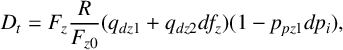 $$ \begin{align} D_t&=F_z \frac{R}{F_{z0}}(q_{dz1}+q_{dz2} d f_z)(1-p_{pz1} d p_i), \end{align} $$
 $$ \begin{align} B_t&=q_{bz1}+q_{bz2} df_z+q_{bz3} {df_z}^2, \end{align} $$
 $$ \begin{align} E_{t 1}&=(q_{ez1}+q_{ez2} df_z+q_{ez3} {df_z}^2)\bigg(1+\frac{2q_{ez4}}{\pi} \arctan (B_t C_t \alpha_1)\bigg), \end{align} $$
 $$ \begin{align} E_{t 2}&=(q_{ez1}+q_{ez2} df_z+q_{ez3} {df_z}^2)\bigg(1+\frac{2 q_{ez4}}{\pi} \arctan (B_t C_t \alpha_2)\bigg). \end{align} $$
Appendix A presents the description of all coefficients in (4.4)–(4.8). The identified values given come from the same example tyre in the literature [Reference Pacejka19] (205/60R15 91 V). Figure 12 illustrates the curves of pneumatic trail varying with slip angle for different inflation pressures.
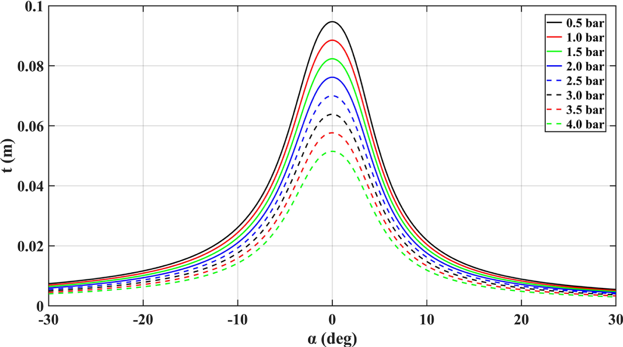
Figure 12 Influence of inflation pressure on the curve of pneumatic trail varying with slip angle.
4.3 Relaxation length
Relaxation length $\sigma $
is usually described as the distance that a tyre rolls before the lateral force builds up to 63% of its steady-state value. It can control the lag of the response of the side force to the input slip angle and is known to be an important factor in causing shimmy. The bifurcation diagram (Figure 13) provides a global picture of the influence of
$\sigma $
is usually described as the distance that a tyre rolls before the lateral force builds up to 63% of its steady-state value. It can control the lag of the response of the side force to the input slip angle and is known to be an important factor in causing shimmy. The bifurcation diagram (Figure 13) provides a global picture of the influence of $\sigma $
on shimmy oscillations. Like t,
$\sigma $
on shimmy oscillations. Like t, $\sigma $
can also make qualitative changes in the two modes, but unlike the previous two tyre characteristics a and t, increasing rather than decreasing
$\sigma $
can also make qualitative changes in the two modes, but unlike the previous two tyre characteristics a and t, increasing rather than decreasing $\sigma $
can weaken shimmy. At 0.6
$\sigma $
can weaken shimmy. At 0.6 $p_{i0}$
, for instance, a slight increase from 0.65 to 0.73 m can cause the tramp mode to disappear, which is shown as the collision of HB3 and HB4, and a further increase to 1.2 m leads to the same result for the yaw mode. If
$p_{i0}$
, for instance, a slight increase from 0.65 to 0.73 m can cause the tramp mode to disappear, which is shown as the collision of HB3 and HB4, and a further increase to 1.2 m leads to the same result for the yaw mode. If $\sigma $
reduces to a very small value (close to zero), in contrast, the two modes merge, that is, HB2 and HB3 collide at a fold point, resulting in the continuous appearance of shimmy from 0 to 325 km/h. In addition, it is worth noticing that with increasing
$\sigma $
reduces to a very small value (close to zero), in contrast, the two modes merge, that is, HB2 and HB3 collide at a fold point, resulting in the continuous appearance of shimmy from 0 to 325 km/h. In addition, it is worth noticing that with increasing $p_i$
, the disappearance points of the yaw mode move to the lower left, which is the opposite to the cases for a and t. Given the fact that
$p_i$
, the disappearance points of the yaw mode move to the lower left, which is the opposite to the cases for a and t. Given the fact that $\sigma $
for an underinflated tyre is typically higher than for an overinflated tyre, the decreases in
$\sigma $
for an underinflated tyre is typically higher than for an overinflated tyre, the decreases in $\sigma $
caused by increasing
$\sigma $
caused by increasing $p_i$
are not conducive to shimmy suppression, but the rises in
$p_i$
are not conducive to shimmy suppression, but the rises in $\sigma $
with lowering
$\sigma $
with lowering $p_i$
may be helpful for shimmy reduction because the tramp mode may not appear. This forms a competitive mechanism with a and t as their decreases for high pressures are beneficial to diminishing shimmy, while their rises for low pressures are the opposite, which means that the consideration of
$p_i$
may be helpful for shimmy reduction because the tramp mode may not appear. This forms a competitive mechanism with a and t as their decreases for high pressures are beneficial to diminishing shimmy, while their rises for low pressures are the opposite, which means that the consideration of $\sigma $
can potentially have a qualitative influence on the bifurcation features in Figure 5. This, therefore, highlights the importance of taking into account various nonlinear tyre behaviour.
$\sigma $
can potentially have a qualitative influence on the bifurcation features in Figure 5. This, therefore, highlights the importance of taking into account various nonlinear tyre behaviour.
Based on Besselink’s improvement [Reference Besselink, Schmeitz and Pacejka5], the following expression is used to model the relationship between relaxation length and inflation pressure:
 $$ \begin{align} \sigma=\frac{K_{y \alpha}}{c_{y0}(1+p_{cy1} dp_i)}, \end{align} $$
where $K_{y\alpha }$
is the cornering stiffness of the tyre obtained in (2.8),
$K_{y\alpha }$
is the cornering stiffness of the tyre obtained in (2.8), $c_{y0}$
is the lateral stiffness of the tyre at nominal vertical force and inflation pressure, and
$c_{y0}$
is the lateral stiffness of the tyre at nominal vertical force and inflation pressure, and $p_{cy1}$
the variation of relaxation length with inflation pressure.
$p_{cy1}$
the variation of relaxation length with inflation pressure.
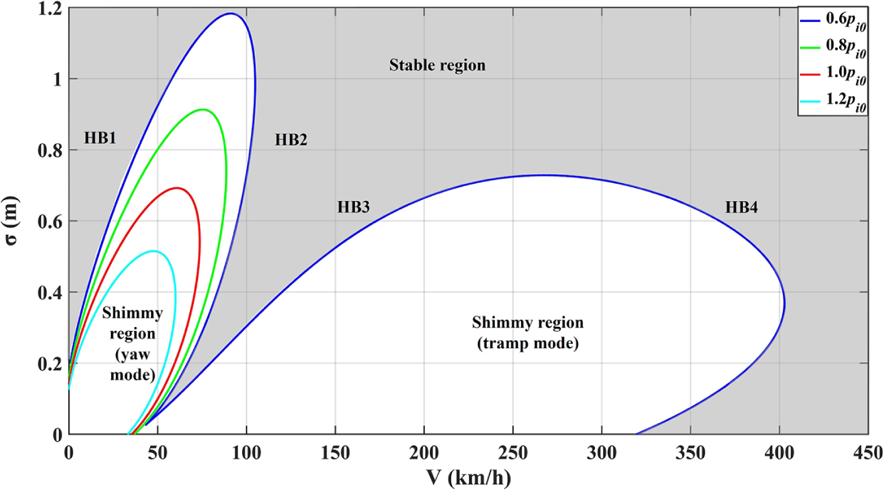
Figure 13 Effect of relaxation length on the Hopf bifurcations for four inflation pressures.
4.4 Vertical stiffness
The vertical stiffness $k_5$
of the tyre strongly depends on inflation pressure and can assume significantly different values even within the range of allowable tyre pressures [Reference Yang, Ballo, Previati and Gobbi35]. Different vertical stiffness leads to substantial changes in shimmy responses. As shown in Figure 14, the curves of the four Hopf bifurcations changing with
$k_5$
of the tyre strongly depends on inflation pressure and can assume significantly different values even within the range of allowable tyre pressures [Reference Yang, Ballo, Previati and Gobbi35]. Different vertical stiffness leads to substantial changes in shimmy responses. As shown in Figure 14, the curves of the four Hopf bifurcations changing with $k_5$
are completely different from the other tyre properties a, t and
$k_5$
are completely different from the other tyre properties a, t and $\sigma $
. At 0.6
$\sigma $
. At 0.6 $p_{i0}$
, with increasing
$p_{i0}$
, with increasing $k_5$
from
$k_5$
from $4\times 10^5$
N/m, the speed range of the yaw mode expands remarkably whilst that of the tramp mode shrinks quickly to zero at
$4\times 10^5$
N/m, the speed range of the yaw mode expands remarkably whilst that of the tramp mode shrinks quickly to zero at $4.39\times 10^5$
N/m, indicating the ending of the tramp mode. The reduction of
$4.39\times 10^5$
N/m, indicating the ending of the tramp mode. The reduction of $k_5$
causes HB2 and HB3 to collide at
$k_5$
causes HB2 and HB3 to collide at $2.55\times 10^5$
N/m, thereby dramatically extending the range of shimmy by merging the two modes. This expansion is also achieved by the curve of HB4, which, as the boundary of the merged mode, has a gentle slope and rapidly exits 350 km/h after
$2.55\times 10^5$
N/m, thereby dramatically extending the range of shimmy by merging the two modes. This expansion is also achieved by the curve of HB4, which, as the boundary of the merged mode, has a gentle slope and rapidly exits 350 km/h after $4\times 10^5$
N/m. As the bifurcation curves in the (V,
$4\times 10^5$
N/m. As the bifurcation curves in the (V, $k_5$
) plane change with inflation pressure, the effect of
$k_5$
) plane change with inflation pressure, the effect of $p_i$
is apparent from the extent of the shimmy region. In particular, as
$p_i$
is apparent from the extent of the shimmy region. In particular, as $p_i$
is increased, compared with the blue curves in Figure 14, other curves are narrower, implying the rapid shrinking of the shimmy region, especially the area where the first mode appears. This is consistent with what is observed in Figure 5.
$p_i$
is increased, compared with the blue curves in Figure 14, other curves are narrower, implying the rapid shrinking of the shimmy region, especially the area where the first mode appears. This is consistent with what is observed in Figure 5.
Figure 14 Effect of vertical stiffness on the Hopf bifurcations at four inflation pressures.
Most notably, the two modes can always be observed for different pressures by changing the value of $k_5$
, which is completely different from other tyre characteristics (a, t and
$k_5$
, which is completely different from other tyre characteristics (a, t and $\sigma $
), in which case, the tramp mode only exists for low pressures (
$\sigma $
), in which case, the tramp mode only exists for low pressures ( $<$
0.8
$<$
0.8 $p_{i0}$
). At
$p_{i0}$
). At $p_{i0}$
, for example, the high-speed mode can emerge through lowering
$p_{i0}$
, for example, the high-speed mode can emerge through lowering $k_5$
from
$k_5$
from $4\times 10^5$
N/m, the value in Figure 4(b), to
$4\times 10^5$
N/m, the value in Figure 4(b), to $2.2\times 10^5$
N/m, the value in Figure 15(a), with remarkably higher peak amplitude than the low-speed mode. In addition, compared with Figure 4(a), the peak amplitude of the tramp angle in Figure 15(a) increases as well (0.14
$2.2\times 10^5$
N/m, the value in Figure 15(a), with remarkably higher peak amplitude than the low-speed mode. In addition, compared with Figure 4(a), the peak amplitude of the tramp angle in Figure 15(a) increases as well (0.14 $^{\circ }$
to 0.41
$^{\circ }$
to 0.41 $^{\circ }$
) with the reduction of
$^{\circ }$
) with the reduction of $k_5$
. Apart from this, after a slight increase from
$k_5$
. Apart from this, after a slight increase from $p_{i0}$
to 1.024
$p_{i0}$
to 1.024 $p_{i0}$
, the two modes are separated from each other as fold bifurcations F1 (
$p_{i0}$
, the two modes are separated from each other as fold bifurcations F1 ( $2.41\times 10^5$
N/m) and F2 (
$2.41\times 10^5$
N/m) and F2 ( $3.19\times 10^5$
N/m) appear. After this separation, the yaw mode bounded by HB1 and HB2 exists for high stiffness (
$3.19\times 10^5$
N/m) appear. After this separation, the yaw mode bounded by HB1 and HB2 exists for high stiffness ( $k_5>$
F2), while the second mode remains in the lower part (
$k_5>$
F2), while the second mode remains in the lower part ( $k_5<2.78\times 10^5$
N/m), leaving the middle region (
$k_5<2.78\times 10^5$
N/m), leaving the middle region ( $2.78\times 10^5 <k_5<$
F2) free of shimmy. Figure 15 compares the bifurcation diagrams before and after the separation. It is noteworthy that although the two modes separate, the residual of the first mode with reduced peak amplitude still exists in Figure 15(b), which is represented in Figure 14 by the small raised portion of the lower red curve with F1 as the vertex. With a further increase in
$2.78\times 10^5 <k_5<$
F2) free of shimmy. Figure 15 compares the bifurcation diagrams before and after the separation. It is noteworthy that although the two modes separate, the residual of the first mode with reduced peak amplitude still exists in Figure 15(b), which is represented in Figure 14 by the small raised portion of the lower red curve with F1 as the vertex. With a further increase in $p_i$
, this portion, as well as F1, gradually disappear (the green curves) and the first mode is farther away from the second mode as F2 moves to F3 (
$p_i$
, this portion, as well as F1, gradually disappear (the green curves) and the first mode is farther away from the second mode as F2 moves to F3 ( $6\times 10^5$
N/m).
$6\times 10^5$
N/m).
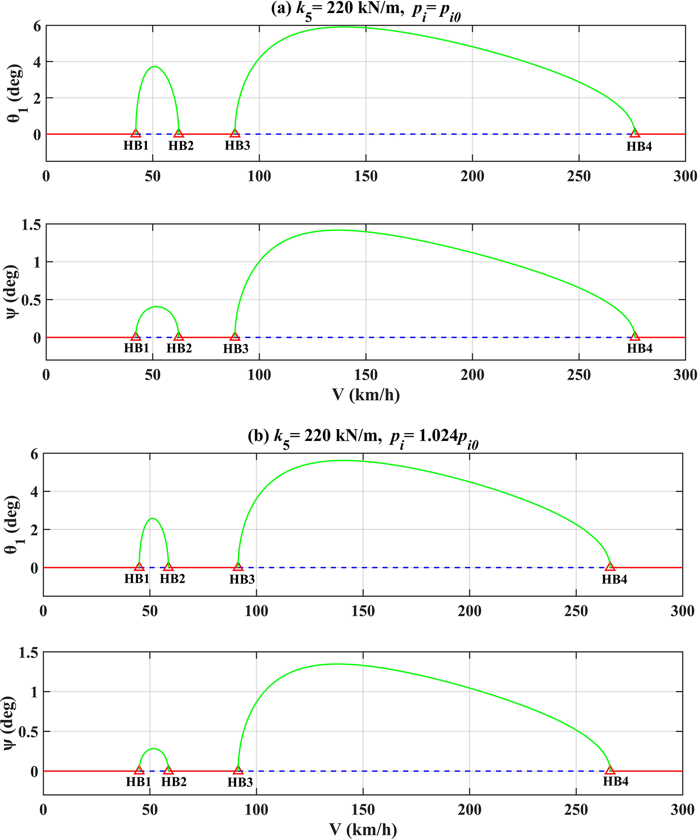
Figure 15 One-parameter bifurcation diagrams for inflation pressures (a) $p_{i0}$
and (b) 1.024
$p_{i0}$
and (b) 1.024 $p_{i0}$
at the same vertical stiffness.
$p_{i0}$
at the same vertical stiffness.
It is known that high pressures strengthen vertical stiffness. If $p_i$
is increased from
$p_i$
is increased from $p_{i0}$
, large
$p_{i0}$
, large $k_5$
, similar to
$k_5$
, similar to $\sigma $
, also has a detrimental effect on mitigating shimmy and undermines the benefit of increasing pressures. This conflicts with the effects of a and t. However, diminished
$\sigma $
, also has a detrimental effect on mitigating shimmy and undermines the benefit of increasing pressures. This conflicts with the effects of a and t. However, diminished $k_5$
due to lowering
$k_5$
due to lowering $p_i$
may also not be conducive to shimmy suppression because the area of the tramp mode can be expanded. In this regard, the effect of
$p_i$
may also not be conducive to shimmy suppression because the area of the tramp mode can be expanded. In this regard, the effect of $k_5$
, together with a and t, conflicts with that of
$k_5$
, together with a and t, conflicts with that of $\sigma $
. These conflicts make the final bifurcation features more unpredictable.
$\sigma $
. These conflicts make the final bifurcation features more unpredictable.
According to Besselink’s work [Reference Besselink, Schmeitz and Pacejka5], a linear function is acceptable to adapt the vertical stiffness for various tyre inflation pressures:
 $$ \begin{align} k_5=k_{5_0}(1+p_{fz1} dp_i), \end{align} $$
where $p_{fz1}$
is the variation parameter of vertical stiffness with inflation pressure. The suggested values of the variation parameters
$p_{fz1}$
is the variation parameter of vertical stiffness with inflation pressure. The suggested values of the variation parameters $p_{cy1}$
and
$p_{cy1}$
and $p_{fz1}$
in (4.9) and (4.10) are obtained from Pacejka [Reference Pacejka19] as an estimate.
$p_{fz1}$
in (4.9) and (4.10) are obtained from Pacejka [Reference Pacejka19] as an estimate.
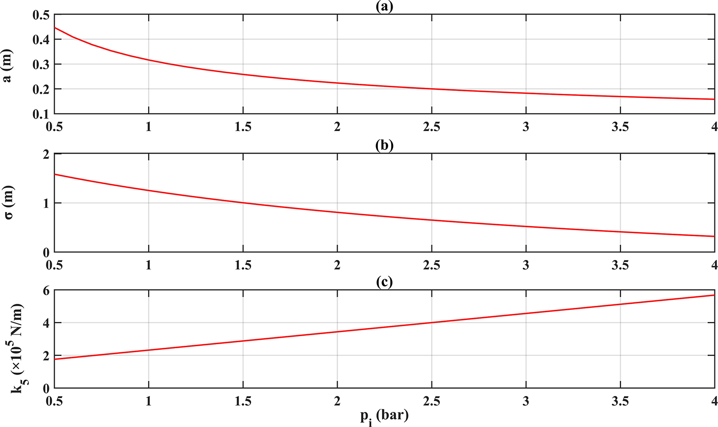
Figure 16 Influence of inflation pressure on (a) half-contact length, (b) relaxation length and (c) vertical stiffness.
Overall, the above two-parameter continuations provided evidence for the strong influence of the four important tyre properties on shimmy oscillations. They were all heavily affected by the tyre inflation pressure, and the mathematical relations between them and pressure changes ${dp}_i$
were developed. The curves of these properties with increasing pressure are illustrated in Figures 12 and 16. It can be concluded that these four properties form two competitive mechanisms: for high pressures (
${dp}_i$
were developed. The curves of these properties with increasing pressure are illustrated in Figures 12 and 16. It can be concluded that these four properties form two competitive mechanisms: for high pressures ( $p_i>p_{i0}$
), diminished a and t, which both help to suppress shimmy, compete with increased
$p_i>p_{i0}$
), diminished a and t, which both help to suppress shimmy, compete with increased $k_5$
and reduced
$k_5$
and reduced $\sigma $
, which both exacerbate shimmy, while for low pressures (
$\sigma $
, which both exacerbate shimmy, while for low pressures ( $p_i<p_{i0}$
), increased
$p_i<p_{i0}$
), increased $\sigma $
, which mitigates shimmy, competes with the other three characteristics, which all worsen shimmy. These mechanisms, hence, suggest that there is a balance between the four characteristics, and a shimmy model needs to correctly balance these competing factors to accurately predict the effects of inflation pressure. In the next section, (4.1)–(4.10) will be added to the model built in Section 2 in order, and additional two-parameter bifurcation studies will be conducted to investigate how the influence of inflation pressure on shimmy oscillations is changed after multiple tyre properties are considered.
$\sigma $
, which mitigates shimmy, competes with the other three characteristics, which all worsen shimmy. These mechanisms, hence, suggest that there is a balance between the four characteristics, and a shimmy model needs to correctly balance these competing factors to accurately predict the effects of inflation pressure. In the next section, (4.1)–(4.10) will be added to the model built in Section 2 in order, and additional two-parameter bifurcation studies will be conducted to investigate how the influence of inflation pressure on shimmy oscillations is changed after multiple tyre properties are considered.
5 Inflation pressure effect considering multiple tyre properties
In this section, two-parameter bifurcation diagrams are computed in the (V, $p_i$
) plane with expressions of half-contact length (HCL) a, pneumatic trail (PT) t, relaxation length (RL)
$p_i$
) plane with expressions of half-contact length (HCL) a, pneumatic trail (PT) t, relaxation length (RL) $\sigma $
and vertical stiffness (VS)
$\sigma $
and vertical stiffness (VS) $k_5$
as functions of pressure changes included in the shimmy model in sequence. As shown in Figure 17, the Hopf bifurcation curves are compared with Figure 5, where only lateral force (LF) is modelled as a function of pressure changes, to highlight the differences after considering multiple tyre properties. The general trend is consistent, that is, increasing pressure can weaken shimmy, and vice versa, which is predictable as the bifurcation diagrams numerically continued in the previous section all agree with it. However, there are still many significant differences between these curves, the most apparent of which is the merge of the yaw and the tramp modes. As shown in the enlarged view in Figure 17(Z2), from the dark blue to the red curves, the inclusion of a causes the curves of HB2 and HB3 to intersect at a cusp (220.5 km/h, 0.03
$k_5$
as functions of pressure changes included in the shimmy model in sequence. As shown in Figure 17, the Hopf bifurcation curves are compared with Figure 5, where only lateral force (LF) is modelled as a function of pressure changes, to highlight the differences after considering multiple tyre properties. The general trend is consistent, that is, increasing pressure can weaken shimmy, and vice versa, which is predictable as the bifurcation diagrams numerically continued in the previous section all agree with it. However, there are still many significant differences between these curves, the most apparent of which is the merge of the yaw and the tramp modes. As shown in the enlarged view in Figure 17(Z2), from the dark blue to the red curves, the inclusion of a causes the curves of HB2 and HB3 to intersect at a cusp (220.5 km/h, 0.03 $p_{i0}$
(0.078 bar)), corresponding to the fusion of the two modes. In addition, as
$p_{i0}$
(0.078 bar)), corresponding to the fusion of the two modes. In addition, as $p_i$
is decreased from
$p_i$
is decreased from $p_{i0}$
, the area bounded by HB1 and HB2 increases in size, indicating a larger range of the yaw mode. In the case of the tramp mode, HB3 and HB4 curves move to the right while the position where the tramp mode disappears remains almost unchanged (256 km/h, 0.7
$p_{i0}$
, the area bounded by HB1 and HB2 increases in size, indicating a larger range of the yaw mode. In the case of the tramp mode, HB3 and HB4 curves move to the right while the position where the tramp mode disappears remains almost unchanged (256 km/h, 0.7 $p_{i0}$
(1.75 bar)). These are consistent with the previous analysis on a (Figure 6), which shows that its increase due to reduced
$p_{i0}$
(1.75 bar)). These are consistent with the previous analysis on a (Figure 6), which shows that its increase due to reduced $p_i$
leads to the expansion of the yaw mode and the right shift of the tramp mode. In contrast, for increased
$p_i$
leads to the expansion of the yaw mode and the right shift of the tramp mode. In contrast, for increased $p_i$
, its decline helps the yaw mode shrink, corresponding to less no-shimmy pressure (1.032
$p_i$
, its decline helps the yaw mode shrink, corresponding to less no-shimmy pressure (1.032 $p_{i0}$
(2.58 bar)) in Figure 17(Z1).
$p_{i0}$
(2.58 bar)) in Figure 17(Z1).
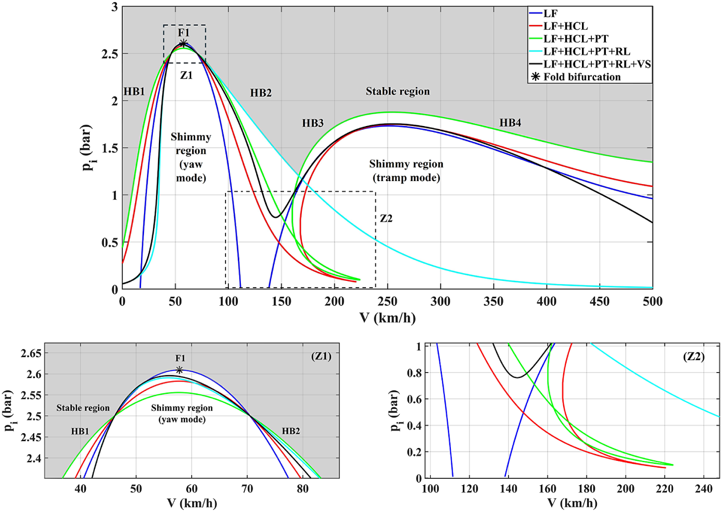
Figure 17 Effect of multiple tyre properties on inflation pressure curves (LF, lateral force; HCL, half-contact length; PT, pneumatic trail; RL, relaxation length; VS, vertical stiffness) and enlarged views (Z1) and (Z2).
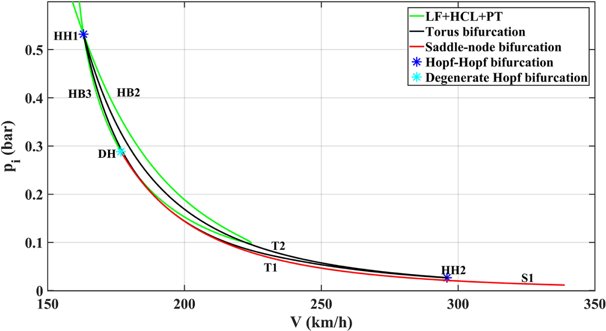
Figure 18 Enlarged bifurcation diagram with torus and saddle-node bifurcation curves included.
For the green curve, the result of involving t is the closed loop formed by the crossing of HB2 and HB3 at 0.2 $1p_{i0}$
(0.53 bar). Based on Figure 8, it is expected that the cross point, as shown in Figure 18, is a double Hopf bifurcation HH1, giving birth to two torus bifurcation curves T1 and T2, and similarly, HB3 becomes subcritical after a degenerate Hopf bifurcation DH, where a saddle-node curve S1 emerges. However, unlike Figure 8, T1 and T2 intersect at another Hopf–Hopf bifurcation HH2 and there is no saddle-node curve detected for HB2. As for the two modes, since t and a have similar effects, the shimmy region further extends when
$1p_{i0}$
(0.53 bar). Based on Figure 8, it is expected that the cross point, as shown in Figure 18, is a double Hopf bifurcation HH1, giving birth to two torus bifurcation curves T1 and T2, and similarly, HB3 becomes subcritical after a degenerate Hopf bifurcation DH, where a saddle-node curve S1 emerges. However, unlike Figure 8, T1 and T2 intersect at another Hopf–Hopf bifurcation HH2 and there is no saddle-node curve detected for HB2. As for the two modes, since t and a have similar effects, the shimmy region further extends when $p_i<p_{i0}$
and narrows when
$p_i<p_{i0}$
and narrows when $p_i>p_{i0}$
. Therefore, although the tramp mode vanishes at higher pressure: 1.88 bar (0.75
$p_i>p_{i0}$
. Therefore, although the tramp mode vanishes at higher pressure: 1.88 bar (0.75 $2p_{i0}$
), thereby maximizing the range of shimmy for pressures less than
$2p_{i0}$
), thereby maximizing the range of shimmy for pressures less than $p_{i0}$
, the pressure at which the system is free of shimmy moves towards the lowest value: 2.56 bar (1.02
$p_{i0}$
, the pressure at which the system is free of shimmy moves towards the lowest value: 2.56 bar (1.02 $4p_{i0}$
).
$4p_{i0}$
).
A qualitative change is made when $\sigma $
is added, shown by the light blue curve, as the tramp mode disappears. This can be attributed to the competitive mechanism discussed before:
$\sigma $
is added, shown by the light blue curve, as the tramp mode disappears. This can be attributed to the competitive mechanism discussed before: $\sigma $
exhibits the opposite effect to a and t. For
$\sigma $
exhibits the opposite effect to a and t. For $p_i<p_{i0}$
, therefore, it leads to the rapid disappearance rather than expansion of the second mode, as well as the delayed onset of the first mode, while for
$p_i<p_{i0}$
, therefore, it leads to the rapid disappearance rather than expansion of the second mode, as well as the delayed onset of the first mode, while for $p_i>p_{i0}$
, this causes shimmy to be suppressed at higher pressure: 2.59 bar (1.036
$p_i>p_{i0}$
, this causes shimmy to be suppressed at higher pressure: 2.59 bar (1.036 $p_{i0}$
), as shown in Figure 17(Z1).
$p_{i0}$
), as shown in Figure 17(Z1).
Due to a similar competition between $k_5$
and
$k_5$
and $\sigma $
for low pressures (
$\sigma $
for low pressures ( $p_i<p_{i0}$
), the tramp mode reappears after the inclusion of
$p_i<p_{i0}$
), the tramp mode reappears after the inclusion of $k_5$
, and has some overlap with the dark blue curve. The effect of
$k_5$
, and has some overlap with the dark blue curve. The effect of $k_5$
is also reflected in the way the two modes intersect: there is no closed loop or cusp. They intersect more smoothly at 0.76 bar (0.304
$k_5$
is also reflected in the way the two modes intersect: there is no closed loop or cusp. They intersect more smoothly at 0.76 bar (0.304 $p_{i0}$
), higher than the values before considering
$p_{i0}$
), higher than the values before considering $k_5$
. In terms of the yaw mode, declined
$k_5$
. In terms of the yaw mode, declined $k_5$
causes HB2 to move to the left, but has a limited influence on HB1. Therefore, in comparison with the light blue curve, the onset of the yaw mode is at nearly the same speed, but the range of velocities declines. However, for
$k_5$
causes HB2 to move to the left, but has a limited influence on HB1. Therefore, in comparison with the light blue curve, the onset of the yaw mode is at nearly the same speed, but the range of velocities declines. However, for $p_i>p_{i0}$
,
$p_i>p_{i0}$
, $k_5$
and
$k_5$
and $\sigma $
both aggravate shimmy, competing with a and t, so shimmy disappears at slightly higher pressure: 2.6 bar (1.04
$\sigma $
both aggravate shimmy, competing with a and t, so shimmy disappears at slightly higher pressure: 2.6 bar (1.04 $p_{i0}$
).
$p_{i0}$
).
Therefore, after all four tyre properties are included in the shimmy model, the Hopf bifurcation curve is significantly different from the initial one. Specifically, for pressures below nominal value, the worsening effects of a, t and $k_5$
on shimmy overwhelm the mitigating effect of
$k_5$
on shimmy overwhelm the mitigating effect of $\sigma $
, so the two shimmy modes merge, implying the disappearance of the intermediate stable region, the onset of shimmy delays and the area of the yaw mode expands. For higher pressures, the suppression effects of a and t are stronger than the exacerbation effects of
$\sigma $
, so the two shimmy modes merge, implying the disappearance of the intermediate stable region, the onset of shimmy delays and the area of the yaw mode expands. For higher pressures, the suppression effects of a and t are stronger than the exacerbation effects of $\sigma $
and
$\sigma $
and $k_5$
. Thus, the shimmy region shrinks and the no-shimmy pressure is slightly reduced.
$k_5$
. Thus, the shimmy region shrinks and the no-shimmy pressure is slightly reduced.
6 Conclusion and future work
The front wheels of a truck with dependent suspension were modelled and analysed in this work to investigate the effect of tyre inflation pressure on shimmy oscillations, with emphasis on the importance of considering multiple nonlinear tyre properties: half-contact length a, pneumatic trail t, relaxation length $\sigma $
and vertical stiffness
$\sigma $
and vertical stiffness $k_5$
, to obtain improved results. Numerical continuation was carried out with the help of toolbox COCO to identify Hopf bifurcations presenting shimmy and to trace their trajectories with parameters of interest. The main conclusions are as follows.
$k_5$
, to obtain improved results. Numerical continuation was carried out with the help of toolbox COCO to identify Hopf bifurcations presenting shimmy and to trace their trajectories with parameters of interest. The main conclusions are as follows.
-
(1) There exist competitive mechanisms in terms of the influence of a, t, $\sigma $
and
$k_5$
on shimmy with pressure changes. When the inflation pressure
$p_i$
is increased to above the nominal value
$p_{i0}$
, the reduction of a and t alleviates shimmy, which forms competition with decreased
$\sigma $
and enhanced
$k_5$
, as they both aggravate shimmy. With lowering
$p_i$
from
$p_{i0}$
, only the rise in
$\sigma $
mitigates shimmy through making the tramp mode disappear, while higher a and t, as well as lower
$k_5$
, all have the effects of exacerbating shimmy.
$\sigma $
and
$k_5$
on shimmy with pressure changes. When the inflation pressure
$p_i$
is increased to above the nominal value
$p_{i0}$
, the reduction of a and t alleviates shimmy, which forms competition with decreased
$\sigma $
and enhanced
$k_5$
, as they both aggravate shimmy. With lowering
$p_i$
from
$p_{i0}$
, only the rise in
$\sigma $
mitigates shimmy through making the tramp mode disappear, while higher a and t, as well as lower
$k_5$
, all have the effects of exacerbating shimmy. -
(2) When only the tyre lateral force is dependent on
$p_i$
, two shimmy modes are identified for low pressures: the yaw mode at medium speed and the tramp mode at high speed, and there is no intersection between the two modes. The shimmy regions shrink significantly with increasing pressure as the tramp mode and then the yaw mode vanish at 0.6
$9p_{i0}$
and 1.04
$p_{i0}$
, respectively. Ultimately, the system is free of shimmy at any speed for high pressures. -
(3) Significant differences appear after the heavy dependence of a, t,
$\sigma $
and
$k_5$
on
$p_i$
is introduced into the extended model. For
$p_i<p_{i0}$
, the effects of a, t and
$k_5$
are major considering the aggravation of shimmy: the shimmy regions expand remarkably with the two modes merging at 0.304
$p_{i0}$
. However, for
$p_i>p_{i0}$
, a and t play a more important role in suppressing shimmy: shimmy happens in a smaller region and disappears at a lower pressure. These differences highlight the importance of considering the balance between these properties to correctly capture the effect of
$p_i$
.


In this work, since insufficient measurement data are available, some estimations for parameters related to pressure and load dependency are made according to different references based on different tyres, and the parameters at nominal conditions, such as $p_{dy1}$
,
$p_{dy1}$
, $p_{ky1}$
and
$p_{ky1}$
and $p_{ey1}$
, are determined to fit the data in Li’s article [Reference Li and Lin16]. Although the extended model established in this work is generic in the context of investigating the effect of inflation pressure on shimmy oscillations with multiple tyre properties included, additional experimental measurements for parametrization can be carried out in the future with the goal of providing better data. In addition, one of the assumptions of this work is that there is no longitudinal slip for the contact patch. Future work can also include extending the shimmy model to consider the effect of combined slip, thereby investigating more realistic vehicle operation scenarios. Finally, vehicles in operation may experience asymmetric pressure settings (for example, if one wheel develops a slow puncture): future work could explore how such asymmetries influence the shimmy response.
$p_{ey1}$
, are determined to fit the data in Li’s article [Reference Li and Lin16]. Although the extended model established in this work is generic in the context of investigating the effect of inflation pressure on shimmy oscillations with multiple tyre properties included, additional experimental measurements for parametrization can be carried out in the future with the goal of providing better data. In addition, one of the assumptions of this work is that there is no longitudinal slip for the contact patch. Future work can also include extending the shimmy model to consider the effect of combined slip, thereby investigating more realistic vehicle operation scenarios. Finally, vehicles in operation may experience asymmetric pressure settings (for example, if one wheel develops a slow puncture): future work could explore how such asymmetries influence the shimmy response.
Acknowledgement
This work is sponsored by Chinese Scholarship Council (File No. 202106830040).
A Values of parameters
The description and values of the parameters in all equations are listed in Table 1, with data sources cited as well. The numbers with superscripts “*” and “+” indicate values that have been modified compared with those in the literature [Reference Pacejka19]: a “+” represents values that have been changed to avoid physically impossible situations like negative pneumatic trail; a “*” indicates values that have been adjusted to make the parameters at nominal pressure match with those in Li’s article [Reference Li and Lin16].


 Open access