


1 Introduction
Constrained fractional optimization problems play a significant role in various domains, including engineering, economics and management. They focus on optimizing a fractional objective function while adhering to specific constraints, allowing for a refined analysis of real-world trade-offs. This paper delves into the mathematical principles and applications of these problems.
We next review recent advances in optimal control theory, highlighting key contributions across various problem classes. Pedregal [Reference Pedregal12] proposed a novel approach to optimal feedback control by treating controls as functions of time and space, yielding optimality conditions via linear transport equations and obstacle problems. Endtmayer et al. [Reference Endtmayer, Langer, Neitzel, Wick and Wollner6] tackled nonlinear partial differential equation (PDE)-constrained problems, presenting a constraint-free optimization framework with adaptive residual-based methods and a posteriori error estimates. Court [Reference Court5] addressed hybrid control under hyperelastic constraints relevant to cardiac mechanics, coupling displacement dynamics with pressure maximization. Wang et al. [Reference Wang, Yu and Song23] reformulated state-constrained parabolic problems into equality-constrained ones, applying an augmented Lagrangian method with semi-smooth Newton solvers and proving super-linear convergence without regularity assumptions. Casas and Yong [Reference Casas and Yong3] analysed semilinear heat equations with memory effects, proving differentiability, stability and second-order sufficiency for optimal control. Fuica et al. [Reference Fuica, Lepe, Otárola and Quero7] examined Navier–Stokes-based control with point sources, leveraging Muckenhoupt weights and specialized Sobolev spaces to derive existence and optimality conditions. Casas and Kunisch [Reference Casas and Kunisch2] explored sparsity-promoting control constraints in semilinear evolution equations, developing tools to handle nonsmoothness and proving stability via second-order analysis. Corella et al. [Reference Corella, Jork and Veliov4] established Hölder and Lipschitz stability for optimal solutions of semilinear parabolic PDEs under perturbations. Finally, Treanţă [Reference Treanţă19] introduced a simplified optimal control formulation involving first-order PDEs and inequality constraints, proving equivalence between saddle points and solutions of the original problem under generalized convexity.
The Riemann–Liouville fractional integral Podlubny [Reference Podlubny13] represented a significant advancement in fractional calculus by extending integration to noninteger orders. This integral allows for the analysis of functions over defined intervals, incorporating memory effects and historical dependencies in various processes. Its versatility makes it valuable across multiple disciplines, effectively modelling complex behaviours often overlooked by traditional integration techniques. By embracing fractional dimensions, it deepens our understanding of intricate systems and their dynamics. Additionally, the concept of fractional action emerges, facilitating the examination of system dynamics through noninteger derivatives. This approach bridges classical mechanics and fractional calculus, enriching our insight into complex behaviours.
In this work, we address the formulation and analysis of a multidimensional fractional optimal control problem grounded in the framework of fractional Lagrangians and Hamiltonians [Reference Toma and Postavaru15], where the fractional nature is embedded in the dynamics of the system. Unlike classical control problems or existing fractional models constrained to one-dimensional settings, our approach generalizes the variational structure to higher-dimensional domains governed by nonlocal, memory-dependent operators, and incorporates inequality constraints directly into the formulation. This generalization poses significant analytical challenges, particularly in establishing necessary optimality conditions under the presence of fractional derivatives. We demonstrate that, under appropriate generalized convexity assumptions, the optimal control problem admits a solution that satisfies a saddle-point condition for an associated Lagrange functional, thereby extending classical control theory to a broader fractional context.
Building on this foundation, we introduce a novel mathematical framework for multidimensional fractional optimal control problems with mixed constraints, incorporating nonvariant curvilinear cost functionals and extended notions of convexity. Starting from the original fractional problem, we develop a modified formulation in which optimality conditions are rigorously derived. A central result of this work is the identification of a correspondence between saddle points in the revised formulation and optimal solutions in the original problem, under suitable convexity assumptions. This connection not only enriches the theoretical understanding of fractional control systems, but also provides a mechanical interpretation of the cost functional in terms of physical work. Additionally, we explore a multi-time setting involving both intrinsic and observer time dimensions, without privileging one over the other, leading to solutions that reflect more complex, anisotropic temporal dynamics. While questions of existence are beyond the scope of this study, we demonstrate the applicability and significance of the proposed framework through a series of illustrative examples based on optimization problems subject to first-order partial differential constraints.
The cited literature [Reference Raymond14, Reference Tröltzsch22] primarily addressed optimal control problems governed by classical PDEs or state constraints within various physical and engineering contexts, including linear and nonlinear systems, parabolic and Navier–Stokes equations, memory effects, and nonsmooth controls. These works contribute significantly to the development of optimality conditions, numerical methods, stability analyses and control constraints in classical (integer-order) frameworks.
In contrast, our work advances the field by formulating and analysing a multidimensional fractional optimal control problem, where the system dynamics are governed by nonlocal fractional differential operators that encode memory and hereditary properties intrinsic to many complex systems. Unlike the primarily one-dimensional or classical PDE constraints seen in the literature [Reference Pedregal12, Reference Treanţă19], our approach extends optimal control theory to fractional models on higher-dimensional spatial domains, embedding the fractional derivatives directly into the variational structure via fractional Lagrangians and Hamiltonians.
Moreover, our formulation explicitly incorporates inequality constraints within this fractional framework and addresses the significant analytical challenges of deriving necessary optimality conditions in the presence of fractional derivatives and nonlocal effects. This leads to novel saddle-point characterizations of solutions under generalized convexity assumptions, which extend and complement classical results. Thus, while building conceptually on the broad themes of optimal control theory explored by Pedregal [Reference Pedregal12] and Treanţă [Reference Treanţă19], our contribution is distinct in the integration of fractional calculus, multidimensional nonlocality and constrained optimization, providing a new avenue for both theoretical analysis and potential applications in systems with fractional dynamics.
The structure of this paper is as follows. Section 2 outlines the notation, definitions and foundational results that are crucial for our analysis. In Section 3, we examine an adapted multidimensional fractional optimal control problem characterized by first-degree partial differential equations and inequality restrictions. We establish connections between the original and modified problems under generalized convexity assumptions. Section 4 examines the relationship between optimal solutions and saddle points related to the Lagrange functional of the modified problem. To demonstrate the effectiveness of our findings, we include several demonstrative examples. In conclusion, Section 5 provides a summary of our findings and reflections.
2 Preliminary definitions and notation
The Riemann–Liouville fractional integral is a pivotal concept in fractional calculus that generalizes the notion of integration to noninteger orders.
Definition 2.1 [Reference Podlubny13]
For a function
 $f(t)$
defined on the interval
$f(t)$
defined on the interval
 $[t_0,t_1]$
and a fractional order
$[t_0,t_1]$
and a fractional order
 $\alpha $
(with
$\alpha $
(with
 $0<\alpha <1$
), the Riemann–Liouville fractional integral is expressed as
$0<\alpha <1$
), the Riemann–Liouville fractional integral is expressed as
 $$ \begin{align*} I^{\alpha}f(t)=\frac{1}{\Gamma(\alpha)}\int_0^tf(\theta)(t-\theta)^{\alpha-1}\,d\theta, \end{align*} $$
with
 $\Gamma $
representing the gamma function
$\Gamma $
representing the gamma function
 $$ \begin{align*} \Gamma(\alpha)=\int_0^{\infty}t^{\alpha-1}e^{-t}\,dt. \end{align*} $$
This integral effectively aggregates the function’s values over time, allowing it to incorporate historical information into its framework. The Riemann–Liouville fractional integral is especially advantageous for modelling processes characterized by memory effects and hereditary behaviours, making it an essential tool across various disciplines, including physics, engineering and applied mathematics.
Definition 2.2 [Reference Toma and Postavaru15]
For a physical system, we define the action as follows:
 $$ \begin{align*} S(s)=\int_{t_0}^{t_1}L(t,s(t),\dot{s}(t))(t_1-t)^{\alpha-1}\,dt. \end{align*} $$
The function
 $L(t,s(t),\dot {s}(t))$
is referred to as the single-time Lagrangian, where
$L(t,s(t),\dot {s}(t))$
is referred to as the single-time Lagrangian, where
 $t\in [t_0,t_1]$
,
$t\in [t_0,t_1]$
,
 $s=(s^1,\ldots ,s^n)$
and
$s=(s^1,\ldots ,s^n)$
and
 $\dot {s}(t)=ds/dt$
. When the fractional coefficient
$\dot {s}(t)=ds/dt$
. When the fractional coefficient
 $\alpha =1$
, the fractional calculus simplifies to ordinary calculus.
$\alpha =1$
, the fractional calculus simplifies to ordinary calculus.
Considering the definitions provided earlier, we present a first-order fractional optimal control problem constrained by partial differential equations, characterized by a nonlinear integral cost
 $$ \begin{align} \min_{s,p}\int_{\Delta}g_{\beta}(t,s(t),p(t))(t_1^{\beta}-t^{\beta})^{\alpha_{\beta}-1}\,dt^{\beta}=0, \end{align} $$
and subject to the following constraints:
 $$ \begin{align} &\Omega^i(t,s(t),p(t))=-\frac{\partial s^i}{\partial t^{\beta}}(t)+V_{\beta}^i(t,s(t),p(t))=0; \end{align} $$
 $$ \begin{align} &W(t,s(t),p(t))\le0; \end{align} $$
 $$ \begin{align} &s(t_1)=s_1,\quad s(t_2)=s_2, \end{align} $$
with
 $s_1$
and
$s_1$
and
 $s_2$
given. We defined
$s_2$
given. We defined
 $t=(t^i)$
,
$t=(t^i)$
,
 $i=1,2,\ldots ,m$
,
$i=1,2,\ldots ,m$
,
 $t\in Y\subset \mathbb {R}^m$
with
$t\in Y\subset \mathbb {R}^m$
with
 $t=t(\tau )$
,
$t=t(\tau )$
,
 $\tau \in [a,b]$
, and the segmented smooth curve
$\tau \in [a,b]$
, and the segmented smooth curve
 $\Delta \subset Y$
joins two m-points
$\Delta \subset Y$
joins two m-points
 $t_1=t(a)$
and
$t_1=t(a)$
and
 $t_2=t(b)$
. We define
$t_2=t(b)$
. We define
 $P\equiv Y\times \mathbb {R}^n\times \mathbb {R}^k$
, and
$P\equiv Y\times \mathbb {R}^n\times \mathbb {R}^k$
, and
 $V_{\beta }:P\to \mathbb {R}^{nm}$
,
$V_{\beta }:P\to \mathbb {R}^{nm}$
,
 $\beta =1,2,\ldots ,n$
and
$\beta =1,2,\ldots ,n$
and
 $W:P\to \mathbb {R}^q$
. Define
$W:P\to \mathbb {R}^q$
. Define
 $\chi $
as the space of segmented differentiable state functions
$\chi $
as the space of segmented differentiable state functions
 $s:Y\to \mathbb {R}^n$
, having the norm defined as follows:
$s:Y\to \mathbb {R}^n$
, having the norm defined as follows:
 $$ \begin{align*} \parallel s\parallel=\parallel s\parallel_{\infty}+\sum_{\beta=1}^m\parallel s_{\beta}\parallel_{\infty}\,,\quad s\in\chi. \end{align*} $$
Define
 $\mathscr {P}$
as the space of segmented continuous control functions
$\mathscr {P}$
as the space of segmented continuous control functions
 $p:Y\to \mathbb {R}^k$
, equipped by the norm
$p:Y\to \mathbb {R}^k$
, equipped by the norm
 $\parallel p\parallel $
. The control function
$\parallel p\parallel $
. The control function
 $p(t)$
is linked to the state function
$p(t)$
is linked to the state function
 $s(t)$
via the first-degree partial differential equations (2.2).
$s(t)$
via the first-degree partial differential equations (2.2).
The set D encompasses all feasible solutions related to the multi-faceted fractional optimal control problem (2.1) and can be described as
 $$ \begin{align*} D=\{(s,p) \mid s\in\chi,p\in \mathscr{P},\Omega(t,s(t),p(t))=0, W(t,s(t),p(t))\le0,s(t_1)=s_1, s(t_2)=s_2\}. \end{align*} $$
Example 2.3. In many physical systems – especially those involving viscoelastic materials, biological tissues or transport in heterogeneous media – the response to external forces is not governed solely by instantaneous interactions, but rather by the entire history of the system’s evolution. These memory-dependent behaviours are inherently nonlocal in time, meaning that past states continue to influence present dynamics. Traditional differential models often fail to capture such effects adequately. In contrast, fractional calculus provides a natural mathematical framework for modelling these complex dynamics by extending classical derivatives to noninteger orders. Fractional operators inherently encode the long-range temporal dependencies that characterize viscoelastic and other memory-rich materials, allowing both strain (deformation) and stress (force per unit area) to be linked through fractional differential equations that more accurately reflect the physics of such systems.
Within this framework, we consider a viscoelastic membrane – such as a soft material, polymer sheet or engineered biological interface – subjected to mechanical loads along two orthogonal directions. The system is modelled using two independent fractional time variables
 $t^1$
and
$t^1$
and
 $t^2$
, which represent anisotropic temporal evolution corresponding to each spatial direction. This formulation captures direction-dependent memory effects, as commonly observed in heterogeneous or layered viscoelastic media. The goal is to determine a control strategy, represented by the stress function
$t^2$
, which represent anisotropic temporal evolution corresponding to each spatial direction. This formulation captures direction-dependent memory effects, as commonly observed in heterogeneous or layered viscoelastic media. The goal is to determine a control strategy, represented by the stress function
 $p(t^\beta )$
,
$p(t^\beta )$
,
 $\beta =1,2$
, that minimizes a cost functional associated with both the accumulated strain energy and the stress effort over the domain. Specifically, we aim to minimize
$\beta =1,2$
, that minimizes a cost functional associated with both the accumulated strain energy and the stress effort over the domain. Specifically, we aim to minimize
 $$ \begin{align*} &\min_{s,p}\int_{0}^{\tau} \bigg( \bigg( \frac{1}{2} s^2(t^1) + \frac{\lambda}{2} p^2(t^1) \bigg)(t_1^{1}-t^{1})^{\alpha_{1}-1}\,dt^1\\ & \quad+ \bigg( \frac{1}{2} s^2(t^2) + \frac{\lambda}{2} p^2(t^2) \bigg)(t_1^{2}-t^{2})^{\alpha_{2}-1}\,dt^2 \bigg)=0, \end{align*} $$
subject to the fractional dynamic constraint
 $$ \begin{align*} \Omega^\beta=-\frac{\partial s}{\partial t^{\beta}}(t^{\beta}) + \frac{1}{b_\beta} \bigg( p(t^{\beta}) + a_\beta \frac{\partial p}{\partial t^{\beta}}(t^{\beta}) \bigg), \quad \beta = 1,2, \end{align*} $$
where
 $a_\beta $
and
$a_\beta $
and
 $b_\beta $
are material-specific constants, and
$b_\beta $
are material-specific constants, and
 $\lambda $
is a weighting parameter that balances the trade-off between minimizing deformation and limiting stress. The boundary conditions are given by
$\lambda $
is a weighting parameter that balances the trade-off between minimizing deformation and limiting stress. The boundary conditions are given by
 $$ \begin{align*} s(0) = s_1, \quad s(\tau) = s_2, \end{align*} $$
corresponding to prescribed deformation states at the start and end of the process. Additionally, a physical constraint on the allowable stress,
 $$ \begin{align*} p(t) \leq p_{\max}, \end{align*} $$
may be imposed to reflect the material’s yield limit, although it is initially omitted in the derivation of optimality conditions and reintroduced later if needed.
This formulation is particularly relevant in applications such as soft robotics, tissue engineering and flexible electronics, where precise control over anisotropic and history-dependent deformation is critical [Reference Caputo and Mainardi1, Reference Li, Chen and Podlubny9, Reference Na and Kim11]. The fractional framework enables a more realistic and flexible description of material response under complex loading, providing insights into optimal strategies for controlling such systems under nonlocal temporal constraints.
To solve this problem, we begin by explicitly formulating the Lagrangian associated with each direction
 $\beta $
, introducing the Lagrange multipliers
$\beta $
, introducing the Lagrange multipliers
 $\phi _{\beta }(t^{\beta })$
. The Lagrangian is defined as
$\phi _{\beta }(t^{\beta })$
. The Lagrangian is defined as
 $$ \begin{align*} \mathcal{L}_{\beta}(s, p, \phi_{\beta})= \frac{1}{2} s^2(t^{\beta}) + \lambda p^2(t^{\beta}) + \phi_{\beta}(t^{\beta}) \bigg( - \frac{\partial s}{\partial t^{\beta}}(t^{\beta}) + \frac{1}{b_{\beta}} \bigg( p(t^{\beta}) +a_{\beta} \frac{\partial p}{\partial t^{\beta}}(t^{\beta}) \bigg) \bigg), \end{align*} $$
where
 $\phi _{\beta }(t^{\beta })$
enforces the dynamic constraint in the
$\phi _{\beta }(t^{\beta })$
enforces the dynamic constraint in the
 $\beta $
th direction. The optimality conditions are then derived by requiring that the Lagrangian satisfies the fractional Euler–Lagrange equation [Reference Toma and Postavaru15]:
$\beta $
th direction. The optimality conditions are then derived by requiring that the Lagrangian satisfies the fractional Euler–Lagrange equation [Reference Toma and Postavaru15]:
 $$ \begin{align*} \frac{\partial \mathcal{L}_{\beta}}{\partial q}-\frac{d}{dt^{\beta}}\bigg(\frac{\partial \mathcal{L}_{\beta}}{\partial \dot{q}}\bigg)=\frac{1-\alpha_{\beta}}{t^{\beta}_1-t^{\beta}}\frac{\partial \mathcal{L}_{\beta}}{\partial \dot{q}}\,,\quad q\in\{s,p\}. \end{align*} $$
After calculations, we obtain the system of equations:
 $$ \begin{align*} &s(t^{\beta})+\frac{d\phi_{\beta}}{dt^{\beta}}(t^{\beta})+\frac{1-\alpha_{\beta}}{t^{\beta}_1-t^{\beta}}\phi_{\beta}(t^{\beta})=0;\\ &2\lambda p(t^{\beta})+\frac{\phi_{\beta}(t^{\beta})}{b_{\beta}}-\frac{a_{\beta}}{b_{\beta}}\frac{d\phi_{\beta}}{dt^{\beta}}(t^{\beta})-\frac{a_{\beta}}{b_{\beta}}\frac{1-\alpha_{\beta}}{t^{\beta}_1-t^{\beta}}\phi_{\beta}(t^{\beta})=0;\\ &-\frac{\partial s}{\partial t^{\beta}}(t^{\beta}) + \frac{1}{b_\beta} \bigg( p(t^{\beta}) + a_\beta \frac{\partial p}{\partial t^{\beta}}(t^{\beta}) \bigg)=0. \end{align*} $$
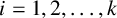
To investigate the behaviour of a viscoelastic system governed by a fractional optimal control model, we numerically solved this system of coupled differential–algebraic equations involving three key variables: the state variable
 $s(t^{\beta })$
, the control variable
$s(t^{\beta })$
, the control variable
 $p(t^{\beta })$
and the adjoint variable
$p(t^{\beta })$
and the adjoint variable
 $\phi (t^{\beta })$
. The model includes a fractional memory effect captured through the parameter
$\phi (t^{\beta })$
. The model includes a fractional memory effect captured through the parameter
 $\alpha _{\beta } \in \{0.7, 0.8, 0.9, 1\}$
, which modulates the nonlocal influence of the past on current dynamics. Physical constants were set to
$\alpha _{\beta } \in \{0.7, 0.8, 0.9, 1\}$
, which modulates the nonlocal influence of the past on current dynamics. Physical constants were set to
 $a_1 = 1$
,
$a_1 = 1$
,
 $a_2 = 0.5$
,
$a_2 = 0.5$
,
 $b_1 = 2$
,
$b_1 = 2$
,
 $b_2 =0.1$
and the weight parameter
$b_2 =0.1$
and the weight parameter
 $\lambda = 3$
, representing the trade-off between minimizing deformation and limiting control effort (stress). The initial conditions
$\lambda = 3$
, representing the trade-off between minimizing deformation and limiting control effort (stress). The initial conditions
 $s(0)=1$
,
$s(0)=1$
,
 $\phi (0)=1$
and
$\phi (0)=1$
and
 $p(0)=0$
were selected to ensure consistency with the system’s structure and constraints.
$p(0)=0$
were selected to ensure consistency with the system’s structure and constraints.
Figures 1(a) and 1(b) display the evolution of the state variable
 $s(t^{\beta })$
over the domain
$s(t^{\beta })$
over the domain
 $t^{\beta } \in [0, 1)$
, showing how it responds to different fractional orders. As
$t^{\beta } \in [0, 1)$
, showing how it responds to different fractional orders. As
 $\alpha _{\beta }$
approaches 1 (the classical case), the system exhibits more localized behaviour, while smaller
$\alpha _{\beta }$
approaches 1 (the classical case), the system exhibits more localized behaviour, while smaller
 $\alpha _{\beta }$
values introduce stronger memory effects, smoothing the response and demonstrating the nonlocal nature of the fractional model. This highlights the role of fractional calculus in accurately modelling viscoelastic materials and systems with temporal memory.
$\alpha _{\beta }$
values introduce stronger memory effects, smoothing the response and demonstrating the nonlocal nature of the fractional model. This highlights the role of fractional calculus in accurately modelling viscoelastic materials and systems with temporal memory.
 $s(t^{\beta })$
,
$s(t^{\beta })$
,
 $\beta =1,2$
, as a function of
$\beta =1,2$
, as a function of
 $t^{\beta }$
for
$t^{\beta }$
for
 $\alpha =0.7$
(purple),
$\alpha =0.7$
(purple),
 $\alpha =0.8$
(blue),
$\alpha =0.8$
(blue),
 $\alpha =0.9$
(brown) and
$\alpha =0.9$
(brown) and
 $\alpha =1$
(opal), with
$\alpha =1$
(opal), with
 $a_1 = 1$
,
$a_1 = 1$
,
 $a_2 = 0.5$
,
$a_2 = 0.5$
,
 $b_1 = 2$
,
$b_1 = 2$
,
 $b_2 =0.1$
,
$b_2 =0.1$
,
 $\lambda = 3$
,
$\lambda = 3$
,
 $s(0)=1$
,
$s(0)=1$
,
 $\phi (0)=1$
and
$\phi (0)=1$
and
 $p(0)=0$
.
$p(0)=0$
.

Remark 2.4. However, in this paper, we do not intend to discuss the dynamics of fractional systems, but rather to develop a formalism capable of establishing optimality conditions for a class of multidimensional fractional optimal control problems. In particular, we demonstrate that, under certain generalized convexity assumptions, the optimal solution corresponds to a saddle point of the Lagrange functional associated with the reformulated problem.
Definition 2.5. A point
 $(s^0,p^0)$
is considered an optimal solution to the fractional optimal control problem (2.1) if, given any
$(s^0,p^0)$
is considered an optimal solution to the fractional optimal control problem (2.1) if, given any
 $(s,p)\in D$
, the subsequent condition holds:
$(s,p)\in D$
, the subsequent condition holds:
 $$ \begin{align} \int_{\Delta}g_{\beta}(t,s(t),p(t))(t_1^{\beta}-t^{\beta})^{\alpha_{\beta}-1}\,dt^{\beta}\ge \int_{\Delta}g_{\beta}(t,s^0(t),p^0(t))(t_1^{\beta}-t^{\beta})^{\alpha_{\beta}-1}\,dt^{\beta}. \end{align} $$
Consider the case where
 $\beta =1,2,\ldots ,m$
and let
$\beta =1,2,\ldots ,m$
and let
 $h_{\beta }:J^1(Y,\mathbb {R}^n)\times \mathbb {R}^k\to \mathbb {R}$
be a continuously differentiable function known as a closed Lagrange 1-form density, defined as
$h_{\beta }:J^1(Y,\mathbb {R}^n)\times \mathbb {R}^k\to \mathbb {R}$
be a continuously differentiable function known as a closed Lagrange 1-form density, defined as
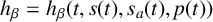 $h_{\beta }=h_{\beta }(t,s(t),s_{a}(t),p(t))$
. In this context,
$h_{\beta }=h_{\beta }(t,s(t),s_{a}(t),p(t))$
. In this context,
 $J^1(Y,\mathbb {R}^n)$
denotes the first-order tangent bundle linked to Y and
$J^1(Y,\mathbb {R}^n)$
denotes the first-order tangent bundle linked to Y and
 $\mathbb {R}^n$
, with
$\mathbb {R}^n$
, with
 $s_a(t)=\partial s/\partial t^a$
. For
$s_a(t)=\partial s/\partial t^a$
. For
 $s\in \chi $
and
$s\in \chi $
and
 $p\in \mathscr {P}$
, we present the subsequent nonpath-dependent curvilinear integral functional
$p\in \mathscr {P}$
, we present the subsequent nonpath-dependent curvilinear integral functional
 $$ \begin{align*} H(s,p)=\int_{\Delta}h_{\beta}(t,s(t),s_{a}(t),p(t))(t_1^{\beta}-t^{\beta})^{\alpha_{\beta}-1}\, dt^{\beta}. \end{align*} $$
Following the framework established by Treanţă in [Reference Treanţă16] (see all definitions provided within), [Reference Treanţă17, Section 2] and [Reference Treanţă18, Section 2.1], and by Treanţă and his co-authors in [Reference Treanţă and Arana-Jiménez20, Section 2], [Reference Treanţă and Arana-Jiménez21, Section 2], [Reference Mititelu and Treanţă10, Definition 2.1], we present the subsequent definitions.
Definition 2.6. If a continuously differentiable function
 $\rho :P\times \mathbb {R}^n\times \mathbb {R}^k\to \mathbb {R}^n$
, with
$\rho :P\times \mathbb {R}^n\times \mathbb {R}^k\to \mathbb {R}^n$
, with
 $$ \begin{align*} \rho=\rho(t,s(t),p(t),s^0(t),p^0(t))=(\rho_i(t,s(t),p(t),s^0(t),p^0(t))), \end{align*} $$
 $i=1,2,\ldots ,n$
, can be found such that
$i=1,2,\ldots ,n$
, can be found such that
 $$ \begin{align} \rho(t,s^0(t),p^0(t),s^0(t),p^0(t))=0, \end{align} $$
for every
 $t\in Y$
,
$t\in Y$
,
 $\rho (t_1)=\rho (t_2)=0$
, and a continuous function
$\rho (t_1)=\rho (t_2)=0$
, and a continuous function
 $\zeta :P\times \mathbb {R}^n\times \mathbb {R}^k\to \mathbb {R}^k$
, with
$\zeta :P\times \mathbb {R}^n\times \mathbb {R}^k\to \mathbb {R}^k$
, with
 $$ \begin{align*} \zeta=\zeta(t,s(t),p(t),s^0(t),p^0(t))=(\zeta_i(t,s(t),p(t),s^0(t),p^0(t))), \end{align*} $$
 $i=1,2,\ldots ,k$
, can be identified such that
$i=1,2,\ldots ,k$
, can be identified such that
 $$ \begin{align} \zeta(t,s^0(t),p^0(t),s^0(t),p^0(t))=0 \end{align} $$
for every
 $t\in Y$
,
$t\in Y$
,
 $\zeta (t_1)=\zeta (t_2)=0$
, and
$\zeta (t_1)=\zeta (t_2)=0$
, and
 $$ \begin{align} H(s,p)-H(s^0,p^0) &\ge \int_{\Delta}\bigg(\frac{\partial h_{\beta}}{\partial s}(t,s^0(t),s_{a}^0(t),p^0(t))\rho +\frac{\partial h_{\beta}}{\partial s_{\beta}}(t,s^0(t),s_{a}^0(t),p^0(t))D_{\beta}\rho\bigg)\nonumber\\ &\quad\times (t_1^{\beta}-t^{\beta})^{\alpha_{\beta}-1}\,dt^{\beta}+\int_{\Delta}\frac{\partial h_{\beta}}{\partial p}(t,s^0(t),s_{a}^0(t),p^0(t))\zeta(t_1^{\beta}-t^{\beta})^{\alpha_{\beta}-1}\,dt^{\beta} \end{align} $$
for any
 $(s,p)\in \chi \times \mathscr {P}$
, then H is deemed invex at
$(s,p)\in \chi \times \mathscr {P}$
, then H is deemed invex at
 $(s^0,p^0)\in \chi \times \mathscr {P}$
with respect to
$(s^0,p^0)\in \chi \times \mathscr {P}$
with respect to
 $\rho $
and
$\rho $
and
 $\zeta $
.
$\zeta $
.
Example 2.7. Consider
 $Y=[0,2]^2$
,
$Y=[0,2]^2$
,
 $\Delta \subset Y$
with
$\Delta \subset Y$
with
 $t\in [t_1,t_2]$
a piecewise smooth curve between the 2-points
$t\in [t_1,t_2]$
a piecewise smooth curve between the 2-points
 $t_1=(0,0)$
and
$t_1=(0,0)$
and
 $t_2=(2,2)$
, with
$t_2=(2,2)$
, with
 $t_1,t_2\in Y$
. Let
$t_1,t_2\in Y$
. Let
 $$ \begin{align*} \chi\times\mathscr{P}&=\bigg\{(s,p) \mid \text{affine piecewise smooth function,} \,s:Y\to\mathbb{R} \\ &\qquad \text{piecewise continuous function}, p:Y\to\mathbb{R} \\ &\qquad \frac{\partial s}{\partial t^1}=\frac{\partial s}{\partial t^2}=2-p, 16-s^2\le0\,,s(0,0)=4\,,s(2,2)=10\bigg\}. \end{align*} $$
We build
 $$ \begin{align*} h(t,s(t),s_{a}(t),p(t))=(c_1+c_2)(2-p)-c_1\frac{\partial s}{\partial t^1}-c_2\frac{\partial s}{\partial t^2}, \end{align*} $$
with
 $c_1$
and
$c_1$
and
 $c_2$
two real constants, and we can write
$c_2$
two real constants, and we can write
 $$ \begin{align} H(s,p)=\int_{\Delta}h(t,s(t),s_{a}(t),p(t))(t_1^{\beta}-t^{\beta})^{\alpha_{\beta}-1}\,dt^{\beta}. \end{align} $$
We define
 $$ \begin{align*} s^0(t)=\tfrac{3}{2}(t^1+t^2)+4\,,\quad p^0(t)=\tfrac{1}{2},\quad t\in Y, \end{align*} $$
and let the functions
 $\rho ,\zeta :Y\times (\mathbb {R}\times \mathbb {R})^2\to \mathbb {R}$
, so that
$\rho ,\zeta :Y\times (\mathbb {R}\times \mathbb {R})^2\to \mathbb {R}$
, so that
 $$ \begin{align*} \rho(t,s(t),p(t),s^0(t),p^0(t))=\begin{cases} s(t)-s^0(t)\,,& t\in Y\backslash\{t_1,t_2\} ,\\ 0\,, & t\in \{t_1,t_2\}, \end{cases} \end{align*} $$
and
 $$ \begin{align*} \zeta(t,s(t),p(t),s^0(t),p^0(t))=\begin{cases} p(t)-p^0(t)\,,& t\in Y\backslash\{t_1,t_2\} ,\\ 0\,, & t\in \{t_1,t_2\}. \end{cases} \end{align*} $$
Using these definitions, we can express (2.9) as
 $$ \begin{align*} H(s,p)=\int_{\Delta}\bigg((c_1+c_2)(2-p)-c_1\frac{\partial s}{\partial t^1}-c_2\frac{\partial s}{\partial t^2}\bigg)(t_1^{\beta}-t^{\beta})^{\alpha_{\beta}-1}\,dt^{\beta}, \end{align*} $$
and we determine by direct calculation
 $H(p^0,s^0)=0$
.
$H(p^0,s^0)=0$
.
Next, we calculate the other derivatives that appear in (2.8),
 $$ \begin{align*} &\int_{\Delta}\frac{\partial h}{\partial s_1}(t,s^0(t),s_{a}^0(t),p^0(t))\frac{\partial\rho}{\partial t^1}(t_1^{\beta}-t^{\beta})^{\alpha_{\beta}-1}\,dt^{\beta} =-c_1\int_{\Delta}\bigg(\frac{\partial s}{\partial t^1}-\frac{3}{2}\bigg)(t_1^{\beta}-t^{\beta})^{\alpha_{\beta}-1}\,dt^{\beta},\\ &\int_{\Delta}\frac{\partial h}{\partial s_2}(t,s^0(t),s_{a}^0(t),p^0(t))\frac{\partial\rho}{\partial t^2}(t_1^{\beta}-t^{\beta})^{\alpha_{\beta}-1}\,dt^{\beta} =-c_2\int_{\Delta}\bigg(\frac{\partial s}{\partial t^2}-\frac{3}{2}\bigg)(t_1^{\beta}-t^{\beta})^{\alpha_{\beta}-1}\,dt^{\beta}, \\ &\int_{\Delta}\frac{\partial h}{\partial p}(t,s^0(t),s_{a}^0(t),p^0(t))\zeta(t_1^{\beta}-t^{\beta})^{\alpha_{\beta}-1}\,dt^{\beta} =-(c_1+c_2)\int_{\Delta}\bigg(p(t)-\frac{1}{2}\bigg)(t_1^{\beta}-t^{\beta})^{\alpha_{\beta}-1}\,dt^{\beta}, \end{align*} $$
and
 $\partial h/\partial s=0$
. Incorporating all these calculations into (2.8), we derive the condition dictated by this inequality. Thus, H is considered invex at
$\partial h/\partial s=0$
. Incorporating all these calculations into (2.8), we derive the condition dictated by this inequality. Thus, H is considered invex at
 $(s^0,p^0)$
in relation to
$(s^0,p^0)$
in relation to
 $\rho $
and
$\rho $
and
 $\zeta $
.
$\zeta $
.
Definition 2.8. If a continuously differentiable function
 $\rho :P\times \mathbb {R}^n\times \mathbb {R}^k\to \mathbb {R}^n$
, with
$\rho :P\times \mathbb {R}^n\times \mathbb {R}^k\to \mathbb {R}^n$
, with
 $$ \begin{align*} \rho=\rho(t,s(t),p(t),s^0(t),p^0(t))=(\rho_i(t,s(t),p(t),s^0(t),p^0(t))), \end{align*} $$
 $i=1,2,\ldots ,n$
, can be found such that
$i=1,2,\ldots ,n$
, can be found such that
 $\rho (t,s^0(t),p^0(t),s^0(t),p^0(t))=0$
for every
$\rho (t,s^0(t),p^0(t),s^0(t),p^0(t))=0$
for every
 $t\in Y$
,
$t\in Y$
,
 $\rho (t_1)=\rho (t_2)=0$
, and a
$\rho (t_1)=\rho (t_2)=0$
, and a
 $C^0$
-class function
$C^0$
-class function
 $\zeta :P\times \mathbb {R}^n\times \mathbb {R}^k\to \mathbb {R}^k$
, with
$\zeta :P\times \mathbb {R}^n\times \mathbb {R}^k\to \mathbb {R}^k$
, with
 $$ \begin{align*} \zeta=\zeta(t,s(t),p(t),s^0(t),p^0(t))=(\zeta_i(t,s(t),p(t),s^0(t),p^0(t))), \end{align*} $$
 $i=1,2,\ldots ,k$
, can be found such that
$i=1,2,\ldots ,k$
, can be found such that
 $\zeta (t,s^0(t),p^0(t),s^0(t),p^0(t))=0$
for every
$\zeta (t,s^0(t),p^0(t),s^0(t),p^0(t))=0$
for every
 $t\in Y$
,
$t\in Y$
,
 $\zeta (t_1)=\zeta (t_2)=0$
, and
$\zeta (t_1)=\zeta (t_2)=0$
, and
 $$ \begin{align*} H(s,p)-H(s^0,p^0)<0 \end{align*} $$
or
 $$ \begin{align*} &\int_{\Delta}\bigg(\frac{\partial h_{\beta}}{\partial s}(t,s^0(t),s_{a}^0(t),p^0(t))\rho +\frac{\partial h_{\beta}}{\partial s_a}(t,s^0(t),s_{a}^0(t),p^0(t))D_a\rho\bigg) (t_1^{\beta}-t^{\beta})^{\alpha_{\beta}-1}\,dt^{\beta} \\ &\quad+\int_{\Delta}\frac{\partial h_{\beta}}{\partial p}(t,s^0(t),s_{a}^0(t),p^0(t))\zeta(t_1^{\beta}-t^{\beta})^{\alpha_{\beta}-1}\,dt^{\beta}<0, \end{align*} $$
or equivalently,
 $$ \begin{align*} H(s,p)-H(s^0,p^0)\ge0 \end{align*} $$
or
 $$ \begin{align} & \int_{\Delta}\bigg(\frac{\partial h_{\beta}}{\partial s}(t,s^0(t),s_{a}^0(t),p^0(t))\rho +\frac{\partial h_{\beta}}{\partial s_a}(t,s^0(t),s_{a}^0(t),p^0(t))D_a\rho\bigg) (t_1^{\beta}-t^{\beta})^{\alpha_{\beta}-1}\,dt^{\beta} \notag \\ &\quad +\int_{\Delta}\frac{\partial h_{\beta}}{\partial p}(t,s^0(t),s_{a}^0(t),p^0(t))\zeta(t_1^{\beta}-t^{\beta})^{\alpha_{\beta}-1}dt^{\beta}\ge 0 \end{align} $$
for any
 $(s,p)\in \chi \times \mathscr {P}$
, then H is deemed pseudoinvex at
$(s,p)\in \chi \times \mathscr {P}$
, then H is deemed pseudoinvex at
 $(s^0,p^0)\in \chi \times \mathscr {P}$
with respect to
$(s^0,p^0)\in \chi \times \mathscr {P}$
with respect to
 $\rho $
and
$\rho $
and
 $\zeta $
.
$\zeta $
.
Example 2.9. Consider
 $Y=[0,2]^2$
,
$Y=[0,2]^2$
,
 $\Delta \subset Y$
with
$\Delta \subset Y$
with
 $t\in [t_1,t_2]$
a piecewise smooth curve between the 2-points
$t\in [t_1,t_2]$
a piecewise smooth curve between the 2-points
 $t_1=(0,0)$
and
$t_1=(0,0)$
and
 $t_2=(2,2)$
, with
$t_2=(2,2)$
, with
 $t_1,t_2\in Y$
. Let
$t_1,t_2\in Y$
. Let
 $$ \begin{align*} \chi\times\mathscr{P}&=\bigg\{(s,p)\mid s:Y\to\mathbb{R}\,, s\, \mathrm{affine\, piecewise\, smooth\, function}, \\ &\qquad p:Y\to\bigg[-\frac{1}{2},\frac{1}{2}\bigg], p\, \mathrm{piecewise\, continuous\, function},\\ &\qquad \frac{\partial s}{\partial t^1}=\frac{\partial s}{\partial t^2}=2-p, 16-s^2\le0\,,s(0,0)=4,s(2,2)=10\bigg\}. \end{align*} $$
We build
 $$ \begin{align} h(t,s(t),s_{a}(t),p(t))=(p(t)-5)^2 \end{align} $$
and we can write
 $$ \begin{align} H(s,p)=\int_{\Delta}h(t,s(t),s_{a}(t),p(t))(t_1^{\beta}-t^{\beta})^{\alpha_{\beta}-1}\,dt^{\beta}. \end{align} $$
We define
 $$ \begin{align*} s^0(t)=\tfrac{3}{2}(t^1+t^2)+4,\quad p^0(t)=\tfrac{1}{2},\quad t\in Y, \end{align*} $$
and let the functions
 $\rho ,\zeta :Y\times (\mathbb {R}\times [-1/2,1/2])^2\to \mathbb {R}$
, so that
$\rho ,\zeta :Y\times (\mathbb {R}\times [-1/2,1/2])^2\to \mathbb {R}$
, so that
 $$ \begin{align*} \rho(t,s(t),p(t),s^0(t),p^0(t))=0 \end{align*} $$
and
 $$ \begin{align*} \zeta(t,s(t),p(t),s^0(t),p^0(t))=\begin{cases} p(t)-p^0(t)\,,& t\in Y\backslash\{t_1,t_2\},\\ 0\,, & t\in \{t_1,t_2\}. \end{cases} \end{align*} $$
Using these definitions, we can express (2.12) in the form of
 $$ \begin{align*} H(s,p)=\int_{\Delta}(p(t)-5)^2(t_1^{\beta}-t^{\beta})^{\alpha_{\beta}-1}\,dt^{\beta} \end{align*} $$
and therefore,
 $$ \begin{align*} H(s,p)-H(s^0,p^0)=\int_{\Delta}\bigg(p(t)-\frac{19}{2}\bigg)\bigg(p(t)-\frac{1}{2}\bigg)(t_1^{\beta}-t^{\beta})^{\alpha_{\beta}-1}\,dt^{\beta}\ge0. \end{align*} $$
According to Definition 2.1, we have
 $\alpha _{\beta } \in (0,1]$
. Since
$\alpha _{\beta } \in (0,1]$
. Since
 $t_1^{\beta }$
is the maximum of
$t_1^{\beta }$
is the maximum of
 $t^{\beta }$
, it follows that
$t^{\beta }$
, it follows that
 $(t_1^{\beta } - t^{\beta }) \ge 0$
and thus,
$(t_1^{\beta } - t^{\beta }) \ge 0$
and thus,
 $(t_1^{\beta } - t^{\beta })^{\alpha _{\beta } - 1} \ge 0$
. This expression is, in fact, an increasing function on the interval
$(t_1^{\beta } - t^{\beta })^{\alpha _{\beta } - 1} \ge 0$
. This expression is, in fact, an increasing function on the interval
 $[0, t_1^{\beta }]$
. As a result, the integrand in the above equation remains nonnegative, implying that the corresponding integral – and hence the area under the graph it defines – is always positive.
$[0, t_1^{\beta }]$
. As a result, the integrand in the above equation remains nonnegative, implying that the corresponding integral – and hence the area under the graph it defines – is always positive.
From (2.11), we calculate
 $$ \begin{align*} \frac{\partial h}{\partial s}=0\,,\quad \frac{\partial h}{\partial s^a}=0\,,\quad \frac{\partial h}{\partial p}=-9. \end{align*} $$
However, using (2.10),
 $$ \begin{align*} & \int_{\Delta}\bigg(\frac{\partial h}{\partial s}(t,s^0(t),s_{a}^0(t),p^0(t))\rho +\frac{\partial h}{\partial s_a}(t,s^0(t),s_{a}^0(t),p^0(t))D_a\rho\bigg)\\ &\quad\times (t_1^{\beta}-t^{\beta})^{\alpha_{\beta}-1}\,dt^{\beta}+\int_{\Delta}\frac{\partial h}{\partial p}(t,s^0(t),s_{a}^0(t),p^0(t))\zeta(t_1^{\beta}-t^{\beta})^{\alpha_{\beta}-1}\,dt^{\beta}\\ &\quad=-9\int_{\Delta}\bigg(p(t)-\frac{1}{2}\bigg)(t_1^{\beta}-t^{\beta})^{\alpha_{\beta}-1}\,dt^{\beta}\ge0, \end{align*} $$
and we conclude that H is pseudoinvex at
 $(s^0,p^0)\in \chi \times \mathscr {P}$
with respect to
$(s^0,p^0)\in \chi \times \mathscr {P}$
with respect to
 $\rho $
and
$\rho $
and
 $\zeta $
.
$\zeta $
.
Theorem 2.10. If
 $(s^0,p^0)\in D$
is an optimal solution, it follows that there exist
$(s^0,p^0)\in D$
is an optimal solution, it follows that there exist
 $\tau \in \mathbb {R}$
, and functions
$\tau \in \mathbb {R}$
, and functions
 $\lambda :Y\to \mathbb {R}^{nm}$
and
$\lambda :Y\to \mathbb {R}^{nm}$
and
 $\gamma :Y\to \mathbb {R}^{\omega }$
, that are piecewise smooth, where
$\gamma :Y\to \mathbb {R}^{\omega }$
, that are piecewise smooth, where
 $\lambda (t)=(\lambda _i^{\beta }(t))$
and
$\lambda (t)=(\lambda _i^{\beta }(t))$
and
 $\gamma (t)=(\gamma ^l(t))$
, in a way that
$\gamma (t)=(\gamma ^l(t))$
, in a way that
 $$ \begin{align*} &\tau\frac{\partial g_{\beta}}{\partial s^i}(t,s^0(t),p^0(t))+\lambda_i^{\beta}\frac{\partial \Omega^i}{\partial s^i}(t,s^0(t),p^0(t))\\ &\quad+\gamma^l\frac{\partial W_l}{\partial s^i}(t,s^0(t),p^0(t))+\frac{\partial \lambda_i^{\beta}}{\partial t^{\beta}}(t)+\frac{1-\alpha_{\beta}}{t_1^{\beta}-t^{\beta}}\lambda_i^{\beta}(t) =0\\ &\tau\frac{\partial g_{\beta}}{\partial p^j}(t,s^0(t),p^0(t))+\lambda_i^{\beta}\frac{\partial \Omega^i}{\partial p^j}(t,s^0(t),p^0(t))\\ &\quad+\gamma^l\frac{\partial W_l}{\partial p^j}(t,s^0(t),p^0(t))=0, \\ &\gamma^lW_l(t,s^0(t),p^0(t))=0,\quad \gamma^l\ge0,\quad \tau\ge0, \end{align*} $$
 $i=1,2,\ldots n$
,
$i=1,2,\ldots n$
,
 $j=1,2,\ldots k$
,
$j=1,2,\ldots k$
,
 $l=1,2,\ldots \omega $
and
$l=1,2,\ldots \omega $
and
 $\beta =1,2,\ldots m$
for all
$\beta =1,2,\ldots m$
for all
 $t\in Y$
, except at points of discontinuity.
$t\in Y$
, except at points of discontinuity.
Proof. We can express the integral cost functional defined along a curvilinear path and the related constraints in a new form by incorporating the variations
 $s(t)+\epsilon _1\overline {s}(t)$
and
$s(t)+\epsilon _1\overline {s}(t)$
and
 $p(t)+\epsilon _2\overline {p}(t)$
, where
$p(t)+\epsilon _2\overline {p}(t)$
, where
 $\epsilon _1$
and
$\epsilon _1$
and
 $\epsilon _2$
are small parameters employed in our variational framework:
$\epsilon _2$
are small parameters employed in our variational framework:
 $$ \begin{align} \mathcal{G}(\epsilon_1,\epsilon_2)&=\int_{\Delta}g_{\beta}(t,s(t)+\epsilon_1\overline{s}(t),s_a(t)+\epsilon_1\overline{s}_a(t),p(t)+\epsilon_2\overline{p}(t)) (t_1^{\beta}-t^{\beta})^{\alpha_{\beta}-1}\,dt^{\beta}, \end{align} $$
 $$ \begin{align} \mathcal{O}(\epsilon_1,\epsilon_2)&=\int_{\Delta}\Omega^i(t,s(t)+\epsilon_1\overline{s}(t),s_a(t)+\epsilon_1\overline{s}_a(t),p(t)+\epsilon_2\overline{p}(t)) (t_1^{\beta}-t^{\beta})^{\alpha_{\beta}-1}\,dt^{\beta}, \nonumber\\ \mathcal{W}(\epsilon_1,\epsilon_2)&=\int_{\Delta}W_l(t,s(t)+\epsilon_1\overline{s}(t),s_a(t)+\epsilon_1\overline{s}_a(t),p(t)+\epsilon_2\overline{p}(t)) (t_1^{\beta}-t^{\beta})^{\alpha_{\beta}-1}\,dt^{\beta}. \end{align} $$
Since
 $(\overline {s},\overline {p})$
serves as a robust weak optimal solution to our problem, it follows that setting
$(\overline {s},\overline {p})$
serves as a robust weak optimal solution to our problem, it follows that setting
 $(\epsilon _1=0,\epsilon _2=0)$
yields a solution to the corresponding optimization problem,
$(\epsilon _1=0,\epsilon _2=0)$
yields a solution to the corresponding optimization problem,
 $$ \begin{align*} \min_{\epsilon_1,\epsilon_2}\mathcal{G}(\epsilon_1,\epsilon_2)=0, \end{align*} $$
considering the constraints
 $$ \begin{align*} &\mathcal{O}(\epsilon_1,\epsilon_2)\le0\,,\quad \mathcal{W}(\epsilon_1,\epsilon_2)=0,\\ &\overline{s}(t_0)=\overline{s}(t_1)=0\,,\quad \overline{s}_{a}(t_0)=\overline{s}_{a}(t_1)=0\,,\quad \overline{p}(t_0)=\overline{p}(t_1)=0. \end{align*} $$
Based on John’s condition [Reference John8], there exist
 $\tau \in \mathbb {R}$
,
$\tau \in \mathbb {R}$
,
 $\lambda :Y\to \mathbb {R}^{nm}$
and
$\lambda :Y\to \mathbb {R}^{nm}$
and
 $\gamma :Y\to \mathbb {R}^{\omega }$
such that
$\gamma :Y\to \mathbb {R}^{\omega }$
such that
 $$ \begin{align} &\tau\nabla \mathcal{G}(0,0)+\lambda_i^{\beta}\nabla \mathcal{O}(0,0)+\gamma^l\nabla \mathcal{W}(0,0)=0, \end{align} $$
 $$ \begin{align} &\gamma^l \mathcal{W}(0,0)=0\,,\quad \gamma^l\ge 0\,,\quad \tau\ge0 , \end{align} $$
where
 $\nabla f(x,y)$
denotes the gradient of f evaluated at the point
$\nabla f(x,y)$
denotes the gradient of f evaluated at the point
 $(x,y)$
.
$(x,y)$
.
By applying the gradient with respect to
 $\epsilon _1$
to (2.13)–(2.14), and making use of (2.15),
$\epsilon _1$
to (2.13)–(2.14), and making use of (2.15),
 $$ \begin{align} \int_{\Delta}\bigg(\tau\frac{\partial g_{\beta}}{\partial s^i}\overline{s}^i+\tau\frac{\partial g_{\beta}}{\partial s^i_a}\overline{s}^i_a+ \lambda_i^{\beta}\frac{\partial \Omega^i}{\partial s^i}\overline{s}^i+\lambda_i^{\beta}\frac{\partial \Omega^i}{\partial s^i_a}\overline{s}^i_a+\gamma^l\frac{\partial W_l}{\partial s^i}\overline{s}^i+\gamma^l\frac{\partial W_l}{\partial s^i_a}\overline{s}^i_a\bigg) (t_1^{\beta}-t^{\beta})^{\alpha_{\beta}-1}\,dt^{\beta}=0. \end{align} $$
Similarly, by applying the gradient with respect to
 $\epsilon _2$
to (2.13)–(2.14), and making use of (2.15),
$\epsilon _2$
to (2.13)–(2.14), and making use of (2.15),
 $$ \begin{align} \int_{\Delta}\bigg(\tau\frac{\partial g_{\beta}}{\partial p^j}\overline{p}^j+\lambda_i^{\beta}\frac{\partial \Omega^i}{\partial p^j}\overline{p}^j+\gamma^l\frac{\partial W_l}{\partial p^j}\overline{p}^j\bigg)(t_1^{\beta}-t^{\beta})^{\alpha_{\beta}-1}\,dt^{\beta}=0. \end{align} $$
By applying integration by parts to (2.17) and rearranging (2.18), we derive the following:
 $$ \begin{align*} \int_{\Delta}\bigg(\tau\frac{\partial g_{\beta}}{\partial s^i}+ \lambda_i^{\beta}\frac{\partial \Omega^i}{\partial s^i}+\frac{\partial\lambda_i^{\beta}}{\partial t^{\beta}}+\gamma^l\frac{\partial W_l}{\partial s^i}+\frac{1-\alpha_{\beta}}{t_1^{\beta}-t^{\beta}}\lambda_i^{\beta}\bigg) \overline{s}^i(t_1^{\beta}-t^{\beta})^{\alpha_{\beta}-1}\,dt^{\beta}=0 \end{align*} $$
and
 $$ \begin{align*} \int_{\Delta}\bigg(\tau\frac{\partial g_{\beta}}{\partial p^j}+\lambda_i^{\beta}\frac{\partial \Omega^i}{\partial p^j}+\gamma^l\frac{\partial W_l}{\partial p^j}\bigg)\overline{p}^j(t_1^{\beta}-t^{\beta})^{\alpha_{\beta}-1}\,dt^{\beta}=0. \end{align*} $$
We arrive at the following result by allowing the variations
 $\overline {s}^i$
and
$\overline {s}^i$
and
 $\overline {p}^j$
to be arbitrary:
$\overline {p}^j$
to be arbitrary:
 $$ \begin{align*} &\tau\frac{\partial g_{\beta}}{\partial s^i}+ \lambda_i^{\beta}\frac{\partial \Omega^i}{\partial s^i}+\frac{\partial\lambda_i^{\beta}}{\partial t^{\beta}}+\gamma^l\frac{\partial W_l}{\partial s^i}+\frac{1-\alpha_{\beta}}{t_1^{\beta}-t^{\beta}}\lambda_i^{\beta}=0, \\ &\tau\frac{\partial g_{\beta}}{\partial p^j}+\lambda_i^{\beta}\frac{\partial \Omega^i}{\partial p^j}+\gamma^l\frac{\partial W_l}{\partial p^j}=0. \end{align*} $$
Beginning with (2.16), we can set
 $$ \begin{align*} \gamma^lW_l=0,\quad \gamma^l\ge 0,\quad \tau\ge0, \end{align*} $$
thus concluding the proof.
3 Conditions for optimality in a multidimensional fractional optimal control problem
In the following section, we examine a general feasible solution
 $(s^0,p^0)\in D$
in the framework of the fractional optimal control problem defined by (2.1). By employing the definitions of
$(s^0,p^0)\in D$
in the framework of the fractional optimal control problem defined by (2.1). By employing the definitions of
 $\rho $
and
$\rho $
and
 $\zeta $
from Definitions 2.6 and 2.8, we present a multi-faceted fractional optimal control problem, formulated as
$\zeta $
from Definitions 2.6 and 2.8, we present a multi-faceted fractional optimal control problem, formulated as
 $$ \begin{align} \min_{s,p}\int_{\Delta}\bigg(\frac{\partial g_{\beta}}{\partial s}(t,s^0(t),p^0(t))\rho+\frac{\partial g_{\beta}}{\partial p}(t,s^0(t),p^0(t))\zeta\bigg)(t_1^{\beta}-t^{\beta})^{\alpha_{\beta}-1}\,dt^{\beta}, \end{align} $$
subject to the following constraints:
 $$ \begin{align*} &\Omega^i(t,s(t),p(t))=-\frac{\partial s^i}{\partial t^{\beta}}(t)+V_{\beta}^i(t,s(t),p(t))=0\,,\quad t\in Y;\\ &W(t,s(t),p(t))\le0\,,\quad i=1,2,\ldots,n,\quad \beta=1,2,\ldots,m;\\ &s(t_1)=s_1,\quad s(t_2)=s_2. \end{align*} $$
It is essential to note that the collection of all admissible solutions for the multi-faceted fractional optimal control problem is similarly represented by D.
Definition 3.1. If
 $(\tilde {s},\tilde {p})\in D$
is regarded as an optimal solution, then it must satisfy the condition for every
$(\tilde {s},\tilde {p})\in D$
is regarded as an optimal solution, then it must satisfy the condition for every
 $(s,p)\in D$
that
$(s,p)\in D$
that
 $$ \begin{align*} &\int_{\Delta}\bigg(\frac{\partial g_{\beta}}{\partial s}(t,s^0(t),p^0(t))\rho(t,s(t),p(t),s^0(t),p^0(t))\\ &\quad+\frac{\partial g_{\beta}}{\partial p}(t,s^0(t),p^0(t))\zeta(t,s(t),p(t),s^0(t),p^0(t))\bigg)(t_1^{\beta}-t^{\beta})^{\alpha_{\beta}-1}\,dt^{\beta}\\ &\ge \int_{\Delta}\bigg(\frac{\partial g_{\beta}}{\partial s}(t,s^0(t),p^0(t))\rho(t,\tilde{s}(t),\tilde{p}(t),s^0(t),p^0(t))\\ &\quad+\frac{\partial g_{\beta}}{\partial p}(t,s^0(t),p^0(t))\zeta(t,\tilde{s}(t),\tilde{p}(t),s^0(t),p^0(t))\bigg)(t_1^{\beta}-t^{\beta})^{\alpha_{\beta}-1}\,dt^{\beta}. \end{align*} $$
Theorem 3.2. Let
 $(s^0,p^0)\in D$
be a normal optimal solution in (2.1) such that
$(s^0,p^0)\in D$
be a normal optimal solution in (2.1) such that
 $$ \begin{align*} &\int_{\Delta}\lambda_i^{\beta}\Omega^i(t,s(t),p(t))(t_1^{\beta}-t^{\beta})^{\alpha_{\beta}-1}\,dt^{\beta},\\ &\int_{\Delta}\gamma^lW_l(t,s^0(t),p^0(t))(t_1^{\beta}-t^{\beta})^{\alpha_{\beta}-1}\,dt^{\beta}, \end{align*} $$
are invex at
 $(s^0,p^0)\in D$
with respect to
$(s^0,p^0)\in D$
with respect to
 $\rho $
and
$\rho $
and
 $\zeta $
. Then,
$\zeta $
. Then,
 $(s^0,p^0)\in D$
constitutes an optimal solution in equation (3.1).
$(s^0,p^0)\in D$
constitutes an optimal solution in equation (3.1).
Proof. By assumption, the relations (2.2)–(2.4) with
 $\tau =1$
, apply to all
$\tau =1$
, apply to all
 $t\in Y$
, except at points of discontinuity. Let us assume, by contradiction, that
$t\in Y$
, except at points of discontinuity. Let us assume, by contradiction, that
 $(s^0,p^0)\in D$
does not qualify as an optimal solution in Definition 3.1. Consequently, there exists
$(s^0,p^0)\in D$
does not qualify as an optimal solution in Definition 3.1. Consequently, there exists
 $(\tilde {s},\tilde {p})\in D$
for which
$(\tilde {s},\tilde {p})\in D$
for which
 $$ \begin{align*} &\int_{\Delta}\bigg(\frac{\partial g_{\beta}}{\partial s}(t,s^0(t),p^0(t))\rho(t,\tilde{s}(t),\tilde{p}(t),s^0(t),p^0(t))\\ &\qquad+\frac{\partial g_{\beta}}{\partial p}(t,s^0(t),p^0(t))\zeta(t,\tilde{s}(t),\tilde{p}(t),s^0(t),p^0(t))\bigg)(t_1^{\beta}-t^{\beta})^{\alpha_{\beta}-1}\,dt^{\beta}\\ &\quad< \int_{\Delta}\bigg(\frac{\partial g_{\beta}}{\partial s}(t,s^0(t),p^0(t))\rho(t,s^0(t),p^0(t),s^0(t),p^0(t))\\ &\qquad+\frac{\partial g_{\beta}}{\partial p}(t,s^0(t),p^0(t))\zeta(t,s^0(t),p^0(t),s^0(t),p^0(t))\bigg)(t_1^{\beta}-t^{\beta})^{\alpha_{\beta}-1}\,dt^{\beta}. \end{align*} $$
Considering that
 $\rho (t,s^0(t),p^0(t),s^0(t),p^0(t))=0$
and
$\rho (t,s^0(t),p^0(t),s^0(t),p^0(t))=0$
and
 $\zeta (t,s^0(t),p^0(t),s^0(t),p^0(t))=0$
, we obtain
$\zeta (t,s^0(t),p^0(t),s^0(t),p^0(t))=0$
, we obtain
 $$ \begin{align} &\int_{\Delta}\bigg(\frac{\partial g_{\beta}}{\partial s}(t,s^0(t),p^0(t))\rho(t,\tilde{s}(t),\tilde{p}(t),s^0(t),p^0(t))\nonumber\\ &\quad+\frac{\partial g_{\beta}}{\partial p}(t,s^0(t),p^0(t))\zeta(t,\tilde{s}(t),\tilde{p}(t),s^0(t),p^0(t))\bigg)(t_1^{\beta}-t^{\beta})^{\alpha_{\beta}-1}\,dt^{\beta}<0. \end{align} $$
Considering the integral
 $$ \begin{align*} \int_{\Delta}\gamma^l(t)W_l(t,s^0(t),p^0(t))(t_1^{\beta}-t^{\beta})^{\alpha_{\beta}-1}\,dt^{\beta} \end{align*} $$
is invex at
 $(s^0,p^0)\in D$
concerning
$(s^0,p^0)\in D$
concerning
 $\rho $
and
$\rho $
and
 $\zeta $
, it implies that
$\zeta $
, it implies that
 $$ \begin{align*} &\int_{\Delta}\gamma^l(t)W_l(t,\tilde{s}(t),\tilde{p}(t))(t_1^{\beta}-t^{\beta})^{\alpha_{\beta}-1}\,dt^{\beta} -\int_{\Delta}\gamma^l(t)W_l(t,s^0(t),p^0(t))(t_1^{\beta}-t^{\beta})^{\alpha_{\beta}-1}\,dt^{\beta}\\ &\quad\ge \int_{\Delta}\gamma^l(t)(W_l)_s(t,s^0(t),p^0(t))\rho(t,\tilde{s}(t),\tilde{p}(t),s^0(t),p^0(t))(t_1^{\beta}-t^{\beta})^{\alpha_{\beta}-1}\,dt^{\beta}\\ &\qquad +\int_{\Delta}\gamma^l(t)(W_l)_p(t,s^0(t),p^0(t))\zeta(t,\tilde{s}(t),\tilde{p}(t),s^0(t),p^0(t))(t_1^{\beta}-t^{\beta})^{\alpha_{\beta}-1}\,dt^{\beta}, \end{align*} $$
where
 $(W_l)_s=\partial W_l/\partial s$
and
$(W_l)_s=\partial W_l/\partial s$
and
 $(W_l)_p=\partial W_l/\partial p$
. Using Theorem 2.10 (
$(W_l)_p=\partial W_l/\partial p$
. Using Theorem 2.10 (
 $\gamma ^lW_l=0$
),
$\gamma ^lW_l=0$
),
 $$ \begin{align} 0&\ge \int_{\Delta}\gamma^l(t)(W_l)_s(t,s^0(t),p^0(t))\rho(t,\tilde{s}(t),\tilde{p}(t),s^0(t),p^0(t))(t_1^{\beta}-t^{\beta})^{\alpha_{\beta}-1}\,dt^{\beta} \nonumber \\ &\quad+\int_{\Delta}\gamma^l(t)(W_l)_p(t,s^0(t),p^0(t))\zeta(t,\tilde{s}(t),\tilde{p}(t),s^0(t),p^0(t))(t_1^{\beta}-t^{\beta})^{\alpha_{\beta}-1}\,dt^{\beta}. \end{align} $$
Following a similar approach to the previous calculation, we use the invexity exhibited by the expression
 $$ \begin{align*} \int_{\Delta}\lambda_i^{\beta}\Omega^i(t,s(t),p(t))(t_1^{\beta}-t^{\beta})^{\alpha_{\beta}-1}\,dt^{\beta}, \end{align*} $$
gaining the inequality
 $$ \begin{align*} &\int_{\Delta}\lambda_i^{\beta}\Omega^i(t,\tilde{s}(t),\tilde{p}(t))(t_1^{\beta}-t^{\beta})^{\alpha_{\beta}-1}\,dt^{\beta} -\int_{\Delta}\lambda_i^{\beta}\Omega^i(t,s^0(t),p^0(t))(t_1^{\beta}-t^{\beta})^{\alpha_{\beta}+1}\,dt^{\beta}\\ &\quad\ge \int_{\Delta}\lambda_i^{\beta}(\Omega^i)_s(t,s^0(t),p^0(t))\rho(t,\tilde{s}(t),\tilde{p}(t),s^0(t),p^0(t))(t_1^{\beta}-t^{\beta})^{\alpha_{\beta}-1}\,dt^{\beta}\\ &\qquad +\int_{\Delta}\lambda_i^{\beta}(\Omega^i)_{s_a}(t,s^0(t),p^0(t))D_{\beta}\rho(t,\tilde{s}(t),\tilde{p}(t),s^0(t),p^0(t))(t_1^{\beta}-t^{\beta})^{\alpha_{\beta}-1}\,dt^{\beta}\\ &\qquad +\int_{\Delta}\lambda_i^{\beta}(\Omega^i)_{p}(t,s^0(t),p^0(t))\zeta(t,\tilde{s}(t),\tilde{p}(t),s^0(t),p^0(t))(t_1^{\beta}-t^{\beta})^{\alpha_{\beta}-1}\,dt^{\beta}, \end{align*} $$
which together with (2.2) gives
 $$ \begin{align*} 0&\ge \int_{\Delta}\lambda_i^{\beta}(\Omega^i)_s(t,s^0(t),p^0(t))\rho(t,\tilde{s}(t),\tilde{p}(t),s^0(t),p^0(t))(t_1^{\beta}-t^{\beta})^{\alpha_{\beta}-1}\,dt^{\beta}\\ &\quad +\int_{\Delta}\lambda_i^{\beta}(\Omega^i)_{s_a}(t,s^0(t),p^0(t))D_{\beta}\rho(t,\tilde{s}(t),\tilde{p}(t),s^0(t),p^0(t))(t_1^{\beta}-t^{\beta})^{\alpha_{\beta}-1}\,dt^{\beta}\\ &\quad +\int_{\Delta}\lambda_i^{\beta}(\Omega^i)_{p}(t,s^0(t),p^0(t))\zeta(t,\tilde{s}(t),\tilde{p}(t),s^0(t),p^0(t))(t_1^{\beta}-t^{\beta})^{\alpha_{\beta}-1}\,dt^{\beta}, \end{align*} $$
or alternatively,
 $$ \begin{align*} 0&\ge \int_{\Delta}\lambda_i^{\beta}(\Omega^i)_s(t,s^0(t),p^0(t))\rho(t,\tilde{s}(t),\tilde{p}(t),s^0(t),p^0(t))(t_1^{\beta}-t^{\beta})^{\alpha_{\beta}-1}\,dt^{\beta}\\ &\quad -\int_{\Delta}\lambda_i^{\beta}D_{\beta}\rho(t,\tilde{s}(t),\tilde{p}(t),s^0(t),p^0(t))(t_1^{\beta}-t^{\beta})^{\alpha_{\beta}-1}\,dt^{\beta}\\ &\quad +\int_{\Delta}\lambda_i^{\beta}(\Omega^i)_{p}(t,s^0(t),p^0(t))\zeta(t,\tilde{s}(t),\tilde{p}(t),s^0(t),p^0(t))(t_1^{\beta}-t^{\beta})^{\alpha_{\beta}-1}\,dt^{\beta}. \end{align*} $$
Integrating this equation by parts,
 $$ \begin{align*} 0&\ge \int_{\Delta}\lambda_i^{\beta}(\Omega^i)_s(t,s^0(t),p^0(t))\rho(t,\tilde{s}(t),\tilde{p}(t),s^0(t),p^0(t))(t_1^{\beta}-t^{\beta})^{\alpha_{\beta}-1}\,dt^{\beta}\\ &\quad +\int_{\Delta}\bigg(D_{\beta}\lambda_i^{\beta}+\frac{1-\alpha_{\beta}}{t_1^{\beta}-t^{\beta}}\lambda_i^{\beta}\bigg)\rho(t,\tilde{s}(t),\tilde{p}(t),s^0(t),p^0(t))(t_1^{\beta}-t^{\beta})^{\alpha_{\beta}-1}\,dt^{\beta}\\ &\quad +\int_{\Delta}\lambda_i^{\beta}(\Omega^i)_{p}(t,s^0(t),p^0(t))\zeta(t,\tilde{s}(t),\tilde{p}(t),s^0(t),p^0(t))(t_1^{\beta}-t^{\beta})^{\alpha_{\beta}-1}\,dt^{\beta}. \end{align*} $$
Adding this equation to (3.3),
 $$ \begin{align*} 0&\ge \int_{\Delta}\bigg(\lambda_i^{\beta}(\Omega^i)_s+D_{\beta}\lambda_i^{\beta}+\frac{1-\alpha_{\beta}}{t_1^{\beta}-t^{\beta}}\lambda_i^{\beta}+\gamma^l(W_l)_s\bigg) \rho(t,\tilde{s}(t),\tilde{p}(t),s^0(t),p^0(t))(t_1^{\beta}-t^{\beta})^{\alpha_{\beta}-1}\,dt^{\beta}\\ &\quad+\int_{\Delta}(\lambda_i^{\beta}(\Omega^i)_{p}+\gamma^l(W_l)_p) \zeta(t,\tilde{s}(t),\tilde{p}(t),s^0(t),p^0(t))(t_1^{\beta}-t^{\beta})^{\alpha_{\beta}-1}\,dt^{\beta}, \end{align*} $$
and by applying Theorem 2.10,
 $$ \begin{align*} &\int_{\Delta}\bigg(\frac{\partial g_{\beta}}{\partial s}(t,s^0(t),p^0(t))\rho(t,\tilde{s}(t),\tilde{p}(t),s^0(t),p^0(t))\\ &\quad+\frac{\partial g_{\beta}}{\partial s}(t,s^0(t),p^0(t))\zeta(t,\tilde{s}(t),\tilde{p}(t),s^0(t),p^0(t))\bigg)(t_1^{\beta}-t^{\beta})^{\alpha_{\beta}-1}\,dt^{\beta}\ge0, \end{align*} $$
because
 $\tau>0$
. Considering (3.2) with
$\tau>0$
. Considering (3.2) with
 $\tau =1$
, we reach a contradiction. Consequently,
$\tau =1$
, we reach a contradiction. Consequently,
 $(s^0,p^0)\in D$
constitutes an optimal solution for (3.1), thus completing the proof.
$(s^0,p^0)\in D$
constitutes an optimal solution for (3.1), thus completing the proof.
Example 3.3. We consider the region
 $Y = [0, 2] \times [0, 2]$
and a curve that is smooth in pieces
$Y = [0, 2] \times [0, 2]$
and a curve that is smooth in pieces
 $\Delta \subset Y$
that connects the points
$\Delta \subset Y$
that connects the points
 $t_1 = (0, 0)$
and
$t_1 = (0, 0)$
and
 $t_2 = (2, 2)$
within Y. Consider
$t_2 = (2, 2)$
within Y. Consider
 $s: Y \to \mathbb {R}$
as an affine function with smooth segments and
$s: Y \to \mathbb {R}$
as an affine function with smooth segments and
 $p: Y \to [-1/2,1/2]$
as a function that is continuous in segments. We will examine the ensuing nonlinear two-dimensional optimal control problem
$p: Y \to [-1/2,1/2]$
as a function that is continuous in segments. We will examine the ensuing nonlinear two-dimensional optimal control problem
 $$ \begin{align} \min_{(s,p)} \int_{\Delta} (p(t) - 5)^2 (t_1^{\beta}-t^{\beta})^{\alpha_{\beta}-1}\,dt^{\beta}, \end{align} $$
constrained by
 $$ \begin{align} \Omega^1&=-\frac{\partial s}{\partial t_1}(t)+2 - p(t)=0, \quad t \in Y, \nonumber\\ \Omega^2&=-\frac{\partial s}{\partial t_2}(t) + 2 - p(t)=0, \\ W&=16 - s^2(t)\le0,\nonumber \end{align} $$
with
 $s(0, 0) = 4$
and
$s(0, 0) = 4$
and
 $s(2, 2) = 10$
.
$s(2, 2) = 10$
.
Let
 $$ \begin{align*} s^0(t) = \tfrac{3}{2}(t^1 + t^2) + 4\,,\quad p^0(t) = \tfrac{1}{2}, \end{align*} $$
for
 $t\in Y$
, representing an admissible solution. We establish the functions
$t\in Y$
, representing an admissible solution. We establish the functions
 $\rho ,\zeta : Y \times (\mathbb {R} \times [-1/2,1/2])^2 \to \mathbb {R}$
as follows:
$\rho ,\zeta : Y \times (\mathbb {R} \times [-1/2,1/2])^2 \to \mathbb {R}$
as follows:
 $$ \begin{align*} \rho(t, s(t), p(t), s^0(t), p^0(t)) =\begin{cases} \frac{7}{4}(s(t) - s^0(t)) & \text{if } t \in Y \setminus \{t_1, t_2\},\\ 0 & \text{if } t \in \{t_1, t_2\}, \end{cases} \end{align*} $$
and
 $$ \begin{align*} \zeta(t, s(t), p(t), s^0(t), p^0(t)) = \begin{cases} \frac{7}{4}(p(t) - p^0(t)) & \text{if } t \in Y \setminus \{t_1, t_2\} ,\\ 0 & \text{if } t \in \{t_1, t_2\}. \end{cases} \end{align*} $$
The modified two-dimensional optimal control problem related to (3.4) is then expressed as follows:
 $$ \begin{align*} \min_{(s,p)} \int_{\Delta}\frac{7}{4} \bigg(\frac{9}{2} - 9p(t)\bigg)(t_1^{\beta}-t^{\beta})^{\alpha_{\beta}-1}\,dt^{\beta}, \end{align*} $$
constrained by
 $$ \begin{align*} \Omega^1&=-\frac{\partial s}{\partial t_1}(t)+2 - p(t), \quad t \in Y, \\ \Omega^2&=-\frac{\partial s}{\partial t_2}(t) + 2 - p(t), \\ W&=16 - s^2(t)\le0, \end{align*} $$
with
 $s(0, 0) = 4$
and
$s(0, 0) = 4$
and
 $s(2, 2) = 10$
.
$s(2, 2) = 10$
.
By applying (2.5), it can be confirmed that
 $(s^0,p^0)$
serves as an optimal solution
$(s^0,p^0)$
serves as an optimal solution
 $$ \begin{align*} \int_{\Delta}\bigg(p(t)-\frac{19}{2}\bigg)\bigg(p(t)-\frac{1}{2}\bigg)(t_1^{\beta}-t^{\beta})^{\alpha_{\beta}-1}\,dt^{\beta}\ge0, \end{align*} $$
with
 $p\in [-1/2,1/2]$
. Since
$p\in [-1/2,1/2]$
. Since
 $t_1^{\beta }$
is the maximum of
$t_1^{\beta }$
is the maximum of
 $t^{\beta }$
, it follows that
$t^{\beta }$
, it follows that
 $(t_1^{\beta } - t^{\beta }) \ge 0$
and thus,
$(t_1^{\beta } - t^{\beta }) \ge 0$
and thus,
 $(t_1^{\beta } - t^{\beta })^{\alpha _{\beta } - 1} \ge 0$
. As a result, the integrand in the above equation remains nonnegative, implying that the corresponding integral is always positive.
$(t_1^{\beta } - t^{\beta })^{\alpha _{\beta } - 1} \ge 0$
. As a result, the integrand in the above equation remains nonnegative, implying that the corresponding integral is always positive.
We check that the functional
 $$ \begin{align*} \int_{\Delta}\gamma^l(t)W_l(t,s(t),p(t))(t_1^{\beta}-t^{\beta})^{\alpha_{\beta}-1}\,dt^{\beta} \end{align*} $$
is invex in
 $(s^0,p^0)$
, that is,
$(s^0,p^0)$
, that is,
 $$ \begin{align*} \int_{\Delta}\gamma^l(t)\bigg((s^0)^2-s^2+2s^0\frac{7}{2}(s-s^0)\bigg)(t_1^{\beta}-t^{\beta})^{\alpha_{\beta}-1}\,dt^{\beta}\ge0, \end{align*} $$
and it is true because
 $s(t)\in [4,10]$
.
$s(t)\in [4,10]$
.
Additionally, the functional
 $$ \begin{align*} \int_{\Delta}\lambda_i^{\beta}(t)\Omega^i_{p}(t,s^0(t),p^0(t))(t_1^{\beta}-t^{\beta})^{\alpha_{\beta}-1}\,dt^{\beta} \end{align*} $$
is invex in
 $(s^0,p^0)$
, because
$(s^0,p^0)$
, because
 $$ \begin{align*} \frac{7}{4}\int_{\Delta}\lambda_i^{\beta}(t)\bigg(\frac{\partial s}{\partial t^{\beta}}(t)-2 +p(t)\bigg)(t_1^{\beta}-t^{\beta})^{\alpha_{\beta}-1}\,dt^{\beta}=0, \end{align*} $$
with
 $\beta =1,2$
, according to (3.5).
$\beta =1,2$
, according to (3.5).
Theorem 3.4. If
 $(s^0, p^0)\in D$
represents an optimal solution pertaining to (3.1), and
$(s^0, p^0)\in D$
represents an optimal solution pertaining to (3.1), and
 $$ \begin{align*} \int_{\Delta}g_{\beta}(t,s(t),p(t))(t_1^{\beta}-t^{\beta})^{\alpha_{\beta}-1}\,dt^{\beta} \end{align*} $$
is pseudoinvex at
 $(s^0, p^0)\in D$
concerning
$(s^0, p^0)\in D$
concerning
 $\rho $
and
$\rho $
and
 $\zeta $
, then
$\zeta $
, then
 $(s^0, p^0)\in D$
serves as an optimal solution for (2.1).
$(s^0, p^0)\in D$
serves as an optimal solution for (2.1).
Proof. Let us consider, for the purpose of contradiction, that
 $(s^0, p^0)\in D$
does not serve as an optimal solution for the control problem presented in (3.1). Consequently, one can find
$(s^0, p^0)\in D$
does not serve as an optimal solution for the control problem presented in (3.1). Consequently, one can find
 $(\tilde {s}, \tilde {p})\in D$
satisfying
$(\tilde {s}, \tilde {p})\in D$
satisfying
 $$ \begin{align*} \int_{\Delta}g_{\beta}(t,\tilde{s}(t),\tilde{p}(t))(t_1^{\beta}-t^{\beta})^{\alpha_{\beta}-1}dt^{\beta}< \int_{\Delta}g_{\beta}(t,s^0(t),p^0(t))(t_1^{\beta}-t^{\beta})^{\alpha_{\beta}-1}\,dt^{\beta}. \end{align*} $$
Given that the functional
 $$ \begin{align*} \int_{\Delta}g_{\beta}(t,s(t),p(t))(t_1^{\beta}-t^{\beta})^{\alpha_{\beta}-1}\,dt^{\beta} \end{align*} $$
is pseudoinvex at
 $(s^0, p^0)\in D$
concerning
$(s^0, p^0)\in D$
concerning
 $\rho $
and
$\rho $
and
 $\zeta $
, the previous inequality leads to
$\zeta $
, the previous inequality leads to
 $$ \begin{align*} &\int_{\Delta}\bigg(\frac{\partial g_{\beta}}{\partial s}(t,s^0(t),p^0(t))\rho(t,\tilde{s}(t),\tilde{p}(t),s^0(t),p^0(t))\\ &\quad+\frac{\partial g_{\beta}}{\partial p}(t,s^0(t),p^0(t))\zeta(t,\tilde{s}(t),\tilde{p}(t),s^0(t),p^0(t))\bigg)(t_1^{\beta}-t^{\beta})^{\alpha_{\beta}-1}\,dt^{\beta}<0. \end{align*} $$
Using the property
 $\rho (t,s^0(t),p^0(t),s^0(t),p^0(t))=0$
and
$\rho (t,s^0(t),p^0(t),s^0(t),p^0(t))=0$
and
 $\zeta (t,s^0(t),p^0(t),s^0(t), p^0(t))=0$
, we can express the previous inequality as
$\zeta (t,s^0(t),p^0(t),s^0(t), p^0(t))=0$
, we can express the previous inequality as
 $$ \begin{align*} &\int_{\Delta}\bigg(\frac{\partial g_{\beta}}{\partial s}(t,s^0(t),p^0(t))\rho(t,\tilde{s}(t),\tilde{p}(t),s^0(t),p^0(t))\\ &\qquad+\frac{\partial g_{\beta}}{\partial p}(t,s^0(t),p^0(t))\zeta(t,\tilde{s}(t),\tilde{p}(t),s^0(t),p^0(t))\bigg)(t_1^{\beta}-t^{\beta})^{\alpha_{\beta}-1}\,dt^{\beta}\\ &\quad<\int_{\Delta}\bigg(\frac{\partial g_{\beta}}{\partial s}(t,s^0(t),p^0(t))\rho(t,s^0(t),p^0(t),s^0(t),p^0(t))\\ &\qquad+\frac{\partial g_{\beta}}{\partial p}(t,s^0(t),p^0(t))\zeta(t,s^0(t),p^0(t),s^0(t),p^0(t))\bigg)(t_1^{\beta}-t^{\beta})^{\alpha_{\beta}-1}\,dt^{\beta}, \end{align*} $$
which contradicts the optimality of
 $(s^0, p^0)\in D$
in (3.1). Therefore, we conclude that
$(s^0, p^0)\in D$
in (3.1). Therefore, we conclude that
 $(s^0, p^0)\in D$
constitutes, in fact, an optimal solution to (2.1), thereby completing the proof.
$(s^0, p^0)\in D$
constitutes, in fact, an optimal solution to (2.1), thereby completing the proof.
4 Criterion for saddle-point optimality
This section establishes a connection among an optimal solution of (2.1) and a saddle point associated with the Lagrange of the revised multidimensional optimal control problem described in (3.1), contingent upon specific generalized convexity assumptions.
Definition 4.1. The Lagrangian related to the revised multidimensional fractional optimal control problem presented in (3.1) is defined as follows:
 $$ \begin{align*} L(s,p,\lambda,\gamma)&=\int_{\Delta}\bigg(\frac{\partial g_{\beta}}{\partial s}(t,s^0(t),p^0(t))\rho(t,s(t),p(t),s^0(t),p^0(t)) \\ &\quad+\frac{\partial g_{\beta}}{\partial p}(t,s^0(t),p^0(t))\zeta(t,s(t),p(t),s^0(t),p^0(t))\\ &\quad + \lambda_i^{\beta}(t)\Omega^i(t,s(t),p(t))+\gamma^l(t)W_l(t,s(t),p(t))\bigg)(t_1^{\beta}-t^{\beta})^{\alpha_{\beta}-1}\,dt^{\beta}. \end{align*} $$
Definition 4.2. A point
 $(s^0,p^0,\tilde {\lambda },\tilde {\gamma }) \in D \times \mathbb {R}^{nm} \times \mathbb {R}^q_+$
is designated as a saddle point of the Lagrangian
$(s^0,p^0,\tilde {\lambda },\tilde {\gamma }) \in D \times \mathbb {R}^{nm} \times \mathbb {R}^q_+$
is designated as a saddle point of the Lagrangian
 $L(s,p,\lambda ,\gamma )$
related to the revised multidimensional optimal control problem presented in (3.1) if it meets the following inequalities:
$L(s,p,\lambda ,\gamma )$
related to the revised multidimensional optimal control problem presented in (3.1) if it meets the following inequalities:
 $$ \begin{align*} L(s^0,p^0,\lambda,\gamma)\le L(s^0,p^0,\tilde{\lambda},\tilde{\gamma})\quad \text{for all}\, (\lambda,\gamma)\in \mathbb{R}^{nm} \times \mathbb{R}^q_+ \end{align*} $$
and
 $$ \begin{align} L(s^0,p^0,\tilde{\lambda},\tilde{\gamma})\le L(s,p,\tilde{\lambda},\tilde{\gamma})\quad \text{for all}\, (s,p)\in D. \end{align} $$
Furthermore, with these definitions in mind, we will formulate and demonstrate two results pertaining to saddle-point optimality.
Theorem 4.3. Assuming that the objective functional
 $$ \begin{align*} \int_{\Delta}g_{\beta}(t,s(t),p(t))(t_1^{\beta}-t^{\beta})^{\alpha_{\beta}-1}\,dt^{\beta} \end{align*} $$
is pseudoinvex at the point
 $(s^0, p^0)\in D$
with respect to
$(s^0, p^0)\in D$
with respect to
 $\rho $
and
$\rho $
and
 $\zeta $
, and that the point
$\zeta $
, and that the point
 $(s^0,p^0,\tilde {\lambda },\tilde {\gamma }) \in D \times \mathbb {R}^{nm} \times \mathbb {R}^q_+$
is designated as a saddle point of the Lagrangian
$(s^0,p^0,\tilde {\lambda },\tilde {\gamma }) \in D \times \mathbb {R}^{nm} \times \mathbb {R}^q_+$
is designated as a saddle point of the Lagrangian
 $L(s,p,\lambda ,\gamma )$
related to the revised multi-faceted optimal control problem stated in (3.1), it can be concluded that
$L(s,p,\lambda ,\gamma )$
related to the revised multi-faceted optimal control problem stated in (3.1), it can be concluded that
 $(s^0, p^0)\in D$
represents a valid optimal solution for (2.1).
$(s^0, p^0)\in D$
represents a valid optimal solution for (2.1).
Proof. Given the hypothesis,
 $(s^0,p^0,\tilde {\lambda },\tilde {\gamma }) \in D \times \mathbb {R}^{nm} \times \mathbb {R}^q_+$
is designated as a saddle point of the Lagrangian
$(s^0,p^0,\tilde {\lambda },\tilde {\gamma }) \in D \times \mathbb {R}^{nm} \times \mathbb {R}^q_+$
is designated as a saddle point of the Lagrangian
 $L(s,p,\lambda ,\gamma )$
related to the revised multi-faceted optimal control problem stated in (3.1). As a result, applying Definition 4.2 yields
$L(s,p,\lambda ,\gamma )$
related to the revised multi-faceted optimal control problem stated in (3.1). As a result, applying Definition 4.2 yields
 $$ \begin{align*} &\int_{\Delta}\bigg(\frac{\partial g_{\beta}}{\partial s}(t,s^0(t),p^0(t))\rho(t,s^0(t),p^0(t),s^0(t),p^0(t))\\ &\qquad+\frac{\partial g_{\beta}}{\partial p}(t,s^0(t),p^0(t))\zeta(t,s^0(t),p^0(t),s^0(t),p^0(t))\\ &\qquad+ \lambda_i^{\beta}(t)\Omega^i(t,s^0(t),p^0(t))+\gamma^l(t)W_l(t,s^0(t),p^0(t))\bigg)(t_1^{\beta}-t^{\beta})^{\alpha_{\beta}-1}\,dt^{\beta}\\ &\quad\le\int_{\Delta}\bigg(\frac{\partial g_{\beta}}{\partial s}(t,s^0(t),p^0(t))\rho(t,s^0(t),p^0(t),s^0(t),p^0(t))\\ &\qquad+\frac{\partial g_{\beta}}{\partial p}(t,s^0(t),p^0(t))\zeta(t,s^0(t),p^0(t),s^0(t),p^0(t))\\ &\qquad+ \tilde{\lambda}_i^{\beta}(t)\Omega^i(t,s^0(t),p^0(t))+\tilde{\gamma}^l(t)W_l(t,s^0(t),p^0(t))\bigg)(t_1^{\beta}-t^{\beta})^{\alpha_{\beta}-1}\,dt^{\beta}, \end{align*} $$
which together with (2.6) and (2.7) gives
 $$ \begin{align*} &\int_{\Delta}( \lambda_i^{\beta}(t)\Omega^i(t,s^0(t),p^0(t))+\gamma^l(t)W_l(t,s^0(t),p^0(t)))(t_1^{\beta}-t^{\beta})^{\alpha_{\beta}-1}\,dt^{\beta}\\ &\quad\le\int_{\Delta}(\tilde{\lambda}_i^{\beta}(t)\Omega^i(t,s^0(t),p^0(t))+\tilde{\gamma}^l(t)W_l(t,s^0(t),p^0(t)))(t_1^{\beta}-t^{\beta})^{\alpha_{\beta}-1}\,dt^{\beta}. \end{align*} $$
Setting
 $\gamma (t)=0$
for
$\gamma (t)=0$
for
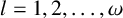 $l=1,2,\ldots ,\omega $
and leveraging the admissibility of
$l=1,2,\ldots ,\omega $
and leveraging the admissibility of
 $(s^0,p^0)$
, we obtain the following results:
$(s^0,p^0)$
, we obtain the following results:
 $$ \begin{align} \int_{\Delta}(\tilde{\lambda}_i^{\beta}(t)\Omega^i(t,s^0(t),p^0(t))+\tilde{\gamma}^l(t)W_l(t,s^0(t),p^0(t)))(t_1^{\beta}-t^{\beta})^{\alpha_{\beta}-1}\,dt^{\beta}\ge0. \end{align} $$
Furthermore, to use proof by contradiction, let us assume that
 $(s^0,p^0)\in D$
does not constitute an optimal solution regarding the optimal control problem stated in (2.1). This implies the existence of
$(s^0,p^0)\in D$
does not constitute an optimal solution regarding the optimal control problem stated in (2.1). This implies the existence of
 $(\tilde {s},\tilde {p})\in D$
for which
$(\tilde {s},\tilde {p})\in D$
for which
 $$ \begin{align*} \int_{\Delta}g_{\beta}(t,\tilde{s}(t),\tilde{p}(t))(t_1^{\beta}-t^{\beta})^{\alpha_{\beta}-1}dt^{\beta}<\int_{\Delta}g_{\beta}(t,s^0(t),p^0(t))(t_1^{\beta}-t^{\beta})^{\alpha_{\beta}-1}\,dt^{\beta}. \end{align*} $$
Given that the functional
 $$ \begin{align*} \int_{\Delta}g_{\beta}(t,s^0(t),p^0(t))(t_1^{\beta}-t^{\beta})^{\alpha_{\beta}-1}\,dt^{\beta} \end{align*} $$
is pseudoinvex at
 $(s^0,p^0)\in D$
with respect to
$(s^0,p^0)\in D$
with respect to
 $\rho $
and
$\rho $
and
 $\zeta $
, the preceding inequality results in the finding that
$\zeta $
, the preceding inequality results in the finding that
 $$ \begin{align*} &\int_{\Delta}\bigg(\frac{\partial g_{\beta}}{\partial s}(t,s^0(t),p^0(t))\rho(t,\tilde{s}(t),\tilde{p}(t),s^0(t),p^0(t))\\ &\quad+\frac{\partial g_{\beta}}{\partial p}(t,s^0(t),p^0(t))\zeta(t,\tilde{s}(t),\tilde{p}(t),s^0(t),p^0(t))\bigg)(t_1^{\beta}-t^{\beta})^{\alpha_{\beta}-1}\,dt^{\beta}<0. \end{align*} $$
Using (2.6) and (2.7), we can express
 $$ \begin{align} &\int_{\Delta}\bigg(\frac{\partial g_{\beta}}{\partial s}(t,s^0(t),p^0(t))\rho(t,\tilde{s}(t),\tilde{p}(t),s^0(t),p^0(t))\nonumber\\ &\qquad+\frac{\partial g_{\beta}}{\partial p}(t,s^0(t),p^0(t))\zeta(t,\tilde{s}(t),\tilde{p}(t),s^0(t),p^0(t))\bigg)(t_1^{\beta}-t^{\beta})^{\alpha_{\beta}-1}\,dt^{\beta}\nonumber\\ &\quad<\int_{\Delta}\bigg(\frac{\partial g_{\beta}}{\partial s}(t,s^0(t),p^0(t))\rho(t,s^0(t),p^0(t),s^0(t),p^0(t))\nonumber\\ &\qquad+\frac{\partial g_{\beta}}{\partial p}(t,s^0(t),p^0(t))\zeta(t,s^0(t),p^0(t),s^0(t),p^0(t))\bigg)(t_1^{\beta}-t^{\beta})^{\alpha_{\beta}-1}\,dt^{\beta}. \end{align} $$
Given that
 $(\tilde {s},\tilde {p})\in D$
, the inequality below holds
$(\tilde {s},\tilde {p})\in D$
, the inequality below holds
 $$ \begin{align*} \int_{\Delta}(\tilde{\lambda}_i^{\beta}(t)\Omega^i(t,\tilde{s}(t),\tilde{p}(t))+\tilde{\gamma}^l(t)W_l(t,\tilde{s}(t),\tilde{p}(t)))(t_1^{\beta}-t^{\beta})^{\alpha_{\beta}-1}\,dt^{\beta}\le0, \end{align*} $$
and combining this result with (4.2),
 $$ \begin{align*} &\int_{\Delta}(\tilde{\lambda}_i^{\beta}(t)\Omega^i(t,\tilde{s}(t),\tilde{p}(t))+\tilde{\gamma}^l(t)W_l(t,\tilde{s}(t),\tilde{p}(t)))(t_1^{\beta}-t^{\beta})^{\alpha_{\beta}-1}\,dt^{\beta}\\ &\quad\le\int_{\Delta}(\tilde{\lambda}_i^{\beta}(t)\Omega^i(t,s^0(t),p^0(t))+\tilde{\gamma}^l(t)W_l(t,s^0(t),p^0(t)))(t_1^{\beta}-t^{\beta})^{\alpha_{\beta}-1}\,dt^{\beta}. \end{align*} $$
The above inequality combined with inequality (4.3) gives
 $$ \begin{align*} &\int_{\Delta}\bigg(\frac{\partial g_{\beta}}{\partial s}(t,s^0(t),p^0(t))\rho(t,\tilde{s}(t),\tilde{p}(t),s^0(t),p^0(t))\\ &\qquad+\frac{\partial g_{\beta}}{\partial p}(t,s^0(t),p^0(t))\zeta(t,\tilde{s},\tilde{p}(t),s^0(t),p^0(t))\\ &\qquad+ \tilde{\lambda}_i^{\beta}(t)\Omega^i(t,\tilde{s}(t),\tilde{p}(t))+\tilde{\gamma}^l(t)W_l(t,\tilde{s}(t),\tilde{p}(t))\bigg)(t_1^{\beta}-t^{\beta})^{\alpha_{\beta}-1}\,dt^{\beta}\\ &\quad<\int_{\Delta}\bigg(\frac{\partial g_{\beta}}{\partial s}(t,s^0(t),p^0(t))\rho(t,s^0(t),p^0(t),s^0(t),p^0(t))\\ &\qquad+\frac{\partial g_{\beta}}{\partial p}(t,s^0(t),p^0(t))\zeta(t,s^0(t),p^0(t),s^0(t),p^0(t))\\ &\qquad+ \tilde{\lambda}_i^{\beta}(t)\Omega^i(t,s^0(t),p^0(t))+\tilde{\gamma}^l(t)W_l(t,s^0(t),p^0(t))\bigg)(t_1^{\beta}-t^{\beta})^{\alpha_{\beta}-1}\,dt^{\beta}, \end{align*} $$
relation that contradicts inequality (4.1). Consequently,
 $(s^0,p^0)\in D$
serves as an optimal solution for the control problem presented in (2.1), thereby completing the proof.
$(s^0,p^0)\in D$
serves as an optimal solution for the control problem presented in (2.1), thereby completing the proof.
Example 4.4. Consider
 $Y=[0,2]^2$
,
$Y=[0,2]^2$
,
 $\Delta \subset Y$
with
$\Delta \subset Y$
with
 $t\in [t_1,t_2]$
a piecewise smooth curve between the 2-points
$t\in [t_1,t_2]$
a piecewise smooth curve between the 2-points
 $t_1=(0,0)$
and
$t_1=(0,0)$
and
 $t_2=(2,2)$
, with
$t_2=(2,2)$
, with
 $t_1,t_2\in Y$
. Let
$t_1,t_2\in Y$
. Let
 $p:Y\to [-1/2,1/2]$
and
$p:Y\to [-1/2,1/2]$
and
 $$ \begin{align*} \frac{\partial s}{\partial t^1}=\frac{\partial s}{\partial t^2}=2-p,\quad 16-s^2\le0,\quad s(0,0)=4,\quad s(2,2)=10. \end{align*} $$
We define
 $$ \begin{align} s^0(t)=\tfrac{3}{2}(t^1+t^2)+4,\quad p^0(t)=\tfrac{1}{2},\quad t\in Y, \end{align} $$
and let the functions
 $\rho ,\zeta :Y\times (\mathbb {R}\times [-1/2,1/2])^2\to \mathbb {R}$
, so that
$\rho ,\zeta :Y\times (\mathbb {R}\times [-1/2,1/2])^2\to \mathbb {R}$
, so that
 $$ \begin{align*} \rho(t,s(t),p(t),s^0(t),p^0(t))=0, \end{align*} $$
and
 $$ \begin{align*} \zeta(t,s(t),p(t),s^0(t),p^0(t))= \begin{cases} p(t)-p^0(t)\,,& t\in Y\backslash\{t_1,t_2\},\\ 0, & t\in \{t_1,t_2\}. \end{cases} \end{align*} $$
As demonstrated in Example 2.7, the modified two-dimensional optimal control problem related to (2.1) can be defined as follows:
 $$ \begin{align*} \min_{(s,p)}\int_{\Delta}-9\bigg(p(t)-\frac{1}{2}\bigg)(t_1^{\beta}-t^{\beta})^{\alpha_{\beta}-1}\,dt^{\beta}, \end{align*} $$
with
 $$ \begin{align*} \frac{\partial s}{\partial t^1}=\frac{\partial s}{\partial t^2}=2-p,\quad 16-s^2\le0,\quad s(0,0)=4,\quad s(2,2)=10. \end{align*} $$
In Example 2.7, we observed that the pair
 $(s^0,p^0)$
defined in (4.4) serves as a saddle point for the Lagrangian
$(s^0,p^0)$
defined in (4.4) serves as a saddle point for the Lagrangian
 $L(s,p,\lambda ,\gamma )$
linked to the revised multi-dimensional optimal control problem outlined in Definition 4.1. So we can write
$L(s,p,\lambda ,\gamma )$
linked to the revised multi-dimensional optimal control problem outlined in Definition 4.1. So we can write
 $$ \begin{align*} L(s,p,\lambda,\gamma)&=\int_{\Delta}\bigg(-9\bigg(p(t)-\frac{1}{2}\bigg) \\ &\quad+ \lambda_i^{\beta}(t)\bigg(-\frac{\partial s}{\partial t^{\beta}}+2-p\bigg)+\gamma^l(t)(16-s^2)\bigg)(t_1^{\beta}-t^{\beta})^{\alpha_{\beta}-1}\,dt^{\beta}, \end{align*} $$
with
 $\beta =1,2$
.
$\beta =1,2$
.
In Example 2.7, the pseudoinvexity of the integral was shown as
 $$ \begin{align*} \int_{\Delta}(p(t)-5)^2(t_1^{\beta}-t^{\beta})^{\alpha_{\beta}-1}\,dt^{\beta}, \end{align*} $$
and consequently, the pair
 $(s^0,p^0)$
represents an optimal solution in (2.1).
$(s^0,p^0)$
represents an optimal solution in (2.1).
Theorem 4.5. Assuming
 $(s^0,p^0)\in D$
represents a normal optimal solution for the fractional optimal control problem outlined in (2.1), and that the functional
$(s^0,p^0)\in D$
represents a normal optimal solution for the fractional optimal control problem outlined in (2.1), and that the functional
 $$ \begin{align} \int_{\Delta}(\tilde{\lambda}_i^{\beta}(t)\Omega^i(t,s(t),p(t))+\tilde{\gamma}^l(t)W_l(t,s(t),p(t)))(t_1^{\beta}-t^{\beta})^{\alpha_{\beta}-1}\,dt^{\beta} \end{align} $$
is invex at
 $(s^0,p^0)\in D$
concerning
$(s^0,p^0)\in D$
concerning
 $\rho $
and
$\rho $
and
 $\zeta $
, then the tuple
$\zeta $
, then the tuple
 $(s^0,p^0, \tilde {\lambda }, \tilde {\gamma }) \in D \times \mathbb {R}^{nm} \times \mathbb {R}^q_+$
serves as a saddle point for the Lagrangian
$(s^0,p^0, \tilde {\lambda }, \tilde {\gamma }) \in D \times \mathbb {R}^{nm} \times \mathbb {R}^q_+$
serves as a saddle point for the Lagrangian
 $L(s, p,\lambda ,\gamma )$
linked to the modified multidimensional fractional optimal control problem outlined in Definition 4.1.
$L(s, p,\lambda ,\gamma )$
linked to the modified multidimensional fractional optimal control problem outlined in Definition 4.1.
Proof. Based on the hypothesis,
 $(s^0,p^0)\in D$
represents a normal optimal solution for the optimal control problem defined in (2.1). Consequently, Theorem 2.10 holds at
$(s^0,p^0)\in D$
represents a normal optimal solution for the optimal control problem defined in (2.1). Consequently, Theorem 2.10 holds at
 $(s^0,p^0)$
for all
$(s^0,p^0)$
for all
 $t\in Y$
, except at points of discontinuity. Here,
$t\in Y$
, except at points of discontinuity. Here,
 $\tilde {\lambda }(t)=(\tilde {\lambda }_i^{\beta }(t))$
and
$\tilde {\lambda }(t)=(\tilde {\lambda }_i^{\beta }(t))$
and
 $\tilde {\gamma }(t)=(\tilde {\gamma }^i(t))$
are piecewise smooth functions, and
$\tilde {\gamma }(t)=(\tilde {\gamma }^i(t))$
are piecewise smooth functions, and
 $\tau =1$
. It can be expressed that
$\tau =1$
. It can be expressed that
 $$ \begin{align*} &\frac{\partial g_{\beta}}{\partial s^i}(t,s^0(t),p^0(t))+\tilde{\lambda}_i^{\beta}\frac{\partial \Omega^i}{\partial s^i}(t,s^0(t),p^0(t))\\ &\quad+\tilde{\gamma}^l\frac{\partial W_l}{\partial s^i}(t,s^0(t),p^0(t))+\frac{\partial \tilde{\lambda}_i^{\beta}}{\partial t^{\beta}}(t)+\frac{1-\alpha_{\beta}}{t_1^{\beta}-t^{\beta}}\tilde{\lambda}_i^{\beta}(t) =0,\\ &\frac{\partial g_{\beta}}{\partial p^j}(t,s^0(t),p^0(t))+\tilde{\lambda}_i^{\beta}\frac{\partial \Omega^i}{\partial p^j}(t,s^0(t),p^0(t))\\ &\quad+\tilde{\gamma}^l\frac{\partial W_l}{\partial p^j}(t,s^0(t),p^0(t))=0, \end{align*} $$
 $i=1,2,\ldots n$
,
$i=1,2,\ldots n$
,
 $j=1,2,\ldots k$
and
$j=1,2,\ldots k$
and
 $\beta =1,2,\ldots m$
. Using the functions
$\beta =1,2,\ldots m$
. Using the functions
 $\rho $
and
$\rho $
and
 $\zeta $
, we can rewrite these equations in the following way:
$\zeta $
, we can rewrite these equations in the following way:
 $$ \begin{align} &\int_{\Delta}\rho(t,s(t),p(t),s^0(t),p^0(t)) \bigg(\frac{\partial g_{\beta}}{\partial s^i}(t,s^0(t),p^0(t))+\tilde{\lambda}_i^{\beta}\frac{\partial \Omega^i}{\partial s^i}(t,s^0(t),p^0(t))\nonumber\\ &\quad+\tilde{\gamma}^l\frac{\partial W_l}{\partial s^i}(t,s^0(t),p^0(t))+\frac{\partial \tilde{\lambda}_i^{\beta}}{\partial t^{\beta}}(t)+\frac{1-\alpha_{\beta}}{t_1^{\beta}-t^{\beta}}\tilde{\lambda}_i^{\beta}(t)\bigg)(t_1^{\beta}-t^{\beta})^{\alpha_{\beta}-1}\,dt^{\beta}=0 \end{align} $$
and
 $$ \begin{align} &\int_{\Delta}\zeta(t,s(t),p(t),s^0(t),p^0(t)) \bigg(\frac{\partial g_{\beta}}{\partial p^j}(t,s^0(t),p^0(t))+\tilde{\lambda}_i^{\beta}\frac{\partial \Omega^i}{\partial p^j}(t,s^0(t),p^0(t))\nonumber\\ &\quad +\tilde{\gamma}^l\frac{\partial W_l}{\partial p^j}(t,s^0(t),p^0(t))\bigg)(t_1^{\beta}-t^{\beta})^{\alpha_{\beta}-1}\,dt^{\beta}=0. \end{align} $$
Integrating by parts (4.6) and using the relation
 $$ \begin{align*} D_{\beta}(\tilde{\lambda}_i^{\beta}(t_1^{\beta}-t^{\beta})^{\alpha_{\beta}-1})=D_{\beta}\tilde{\lambda}_i^{\beta}(t_1^{\beta}-t^{\beta})^{\alpha_{\beta}-1}+\tilde{\lambda}_i^{\beta}\frac{1-\alpha_{\beta}}{t_1^{\beta}-t^{\beta}}(t_1^{\beta}-t^{\beta})^{\alpha_{\beta}-1}, \end{align*} $$
we get
 $$ \begin{align*} &\int_{\Delta}\rho(t,s(t),p(t),s^0(t),p^0(t))\bigg(\frac{\partial g_{\beta}}{\partial s^i}(t,s^0(t),p^0(t))\\ &\quad+\tilde{\lambda}_i^{\beta}\frac{\partial \Omega^i}{\partial s^i}(t,s^0(t),p^0(t))+\tilde{\gamma}^l\frac{\partial W_l}{\partial s^i}(t,s^0(t),p^0(t))\bigg)(t_1^{\beta}-t^{\beta})^{\alpha_{\beta}-1}\,dt^{\beta}\\ &\quad-\int_{\Delta}\tilde{\lambda}_i^{\beta}(t)D_{\beta}\rho(t,s(t),p(t),s^0(t),p^0(t))(t_1^{\beta}-t^{\beta})^{\alpha_{\beta}-1}\,dt^{\beta}=0. \end{align*} $$
Using the fact that the function in (4.5) is invex at
 $(s^0,p^0)\in D$
in relation to
$(s^0,p^0)\in D$
in relation to
 $\rho $
and
$\rho $
and
 $\zeta $
, we write
$\zeta $
, we write
 $$ \begin{align} &\int_{\Delta}(\tilde{\lambda}_i^{\beta}(t)\Omega^i(t,s(t),p(t))+\tilde{\gamma}^l(t)W_l(t,s(t),p(t)))(t_1^{\beta}-t^{\beta})^{\alpha_{\beta}-1}\,dt^{\beta}\nonumber\\ &\qquad-\int_{\Delta}(\tilde{\lambda}_i^{\beta}(t)\Omega^i(t,s^0(t),p^0(t))+\tilde{\gamma}^l(t)W_l(t,s^0(t),p^0(t)))(t_1^{\beta}-t^{\beta})^{\alpha_{\beta}-1}\,dt^{\beta}\nonumber\\ &\quad\ge \int_{\Delta}\rho(t,s(t),p(t),s^0(t),p^0(t))\bigg(\tilde{\lambda}_i^{\beta}(t)\frac{\partial\Omega^i}{\partial s^i}(t,s^0(t),p^0(t))\nonumber\\ &\qquad+\tilde{\gamma}^l(t)\frac{\partial W_l}{\partial s^i}(t,s^0(t),p^0(t))-\tilde{\lambda}_i^{\beta}(t)D_{\beta}\rho\bigg)(t_1^{\beta}-t^{\beta})^{\alpha_{\beta}-1}\,dt^{\beta}\nonumber\\ &\qquad+\int_{\Delta}\bigg(\tilde{\lambda}_i^{\beta}(t)\frac{\partial\Omega^i}{\partial p^j}(t,s^0(t),p^0(t))+\tilde{\gamma}^l(t)\frac{\partial W_l}{\partial p^j}(t,s^0(t),p^0(t))\bigg)\nonumber\\ &\qquad\times\zeta(t,s(t),p(t),s^0(t),p^0(t))(t_1^{\beta}-t^{\beta})^{\alpha_{\beta}-1}\,dt^{\beta}. \end{align} $$
This result follows from (2.8) using
 ${\partial \Omega ^i}/{\partial s_\beta } = -1$
and
${\partial \Omega ^i}/{\partial s_\beta } = -1$
and
 ${\partial W_l}/{\partial s_\beta } = 0$
(see (2.2)–(2.3)).
${\partial W_l}/{\partial s_\beta } = 0$
(see (2.2)–(2.3)).
 $$ \begin{align*} &\int_{\Delta}(\tilde{\lambda}_i^{\beta}(t)\Omega^i(t,s(t),p(t))+\tilde{\gamma}^l(t)W_l(t,s(t),p(t)))(t_1^{\beta}-t^{\beta})^{\alpha_{\beta}-1}\,dt^{\beta}\\ &\qquad-\int_{\Delta}(\tilde{\lambda}_i^{\beta}(t)\Omega^i(t,s^0(t),p^0(t))+\tilde{\gamma}^l(t)W_l(t,s^0(t),p^0(t)))(t_1^{\beta}-t^{\beta})^{\alpha_{\beta}-1}\,dt^{\beta}\\ &\quad\ge -\int_{\Delta}\rho(t,s(t),p(t),s^0(t),p^0(t))\frac{\partial g_{\beta}}{\partial s^i}(t,s^0(t),p^0(t))(t_1^{\beta}-t^{\beta})^{\alpha_{\beta}-1}\,dt^{\beta}\\ &\qquad -\int_{\Delta}\zeta(t,s(t),p(t),s^0(t),p^0(t))\frac{\partial g_{\beta}}{\partial p^j}(t,s^0(t),p^0(t))(t_1^{\beta}-t^{\beta})^{\alpha_{\beta}-1}\,dt^{\beta}.\end{align*} $$
With the help of (2.6) and (2.7), we reformulate the above inequality in
 $$ \begin{align*} &\int_{\Delta}(\tilde{\lambda}_i^{\beta}(t)\Omega^i(t,s(t),p(t))+\tilde{\gamma}^l(t)W_l(t,s(t),p(t)))(t_1^{\beta}-t^{\beta})^{\alpha_{\beta}-1}\,dt^{\beta}\\ &\qquad+\int_{\Delta}\rho(t,s(t),p(t),s^0(t),p^0(t))\frac{\partial g_{\beta}}{\partial s^i}(t,s^0(t),p^0(t))(t_1^{\beta}-t^{\beta})^{\alpha_{\beta}-1}\,dt^{\beta}\\ &\qquad+\int_{\Delta}\zeta(t,s(t),p(t),s^0(t),p^0(t))\frac{\partial g_{\beta}}{\partial p^j}(t,s^0(t),p^0(t))(t_1^{\beta}-t^{\beta})^{\alpha_{\beta}-1}\,dt^{\beta}\\ &\quad\ge\int_{\Delta}(\tilde{\lambda}_i^{\beta}(t)\Omega^i(t,s(t),p(t))+\tilde{\gamma}^l(t)W_l(t,s(t),p(t)))(t_1^{\beta}-t^{\beta})^{\alpha_{\beta}-1}\,dt^{\beta}\\ &\qquad+\int_{\Delta}\rho(t,s^0(t),p^0(t),s^0(t),p^0(t))\frac{\partial g_{\beta}}{\partial s^i}(t,s^0(t),p^0(t))(t_1^{\beta}-t^{\beta})^{\alpha_{\beta}-1}\,dt^{\beta}\\ &\qquad+\int_{\Delta}\zeta(t,s^0(t),p^0(t),s^0(t),p^0(t))\frac{\partial g_{\beta}}{\partial p^j}(t,s^0(t),p^0(t))(t_1^{\beta}-t^{\beta})^{\alpha_{\beta}-1}\,dt^{\beta}, \end{align*} $$
that is,
 $$ \begin{align*} L(s,p,\tilde{\lambda},\tilde{\gamma})\ge L(s^0,p^0,\tilde{\lambda},\tilde{\gamma})\quad \text{for all}\, (s,p)\in D. \end{align*} $$
Starting from the inequality
 $$ \begin{align*} \int_{\Delta}(\lambda_i^{\beta}(t)\Omega^i(t,s^0(t),p^0(t))+\gamma^l(t)W_l(t,s^0(t),p^0(t)))(t_1^{\beta}-t^{\beta})^{\alpha_{\beta}-1}\,dt^{\beta}\le0 \end{align*} $$
for any
 $(\lambda , \mu ) \in \mathbb {R}^{nm} \times \mathbb {R}^q_+$
. By taking into account the feasibility of
$(\lambda , \mu ) \in \mathbb {R}^{nm} \times \mathbb {R}^q_+$
. By taking into account the feasibility of
 $(s^0,p^0)$
, we derive the following outcome:
$(s^0,p^0)$
, we derive the following outcome:
 $$ \begin{align*} &\int_{\Delta}(\lambda_i^{\beta}(t)\Omega^i(t,s^0(t),p^0(t))+\gamma^l(t)W_l(t,s^0(t),p^0(t)))(t_1^{\beta}-t^{\beta})^{\alpha_{\beta}-1}\,dt^{\beta}\\ &\quad\le\int_{\Delta}(\tilde{\lambda}_i^{\beta}(t)\Omega^i(t,s^0(t),p^0(t))+\tilde{\gamma}^l(t)W_l(t,s^0(t),p^0(t)))(t_1^{\beta}-t^{\beta})^{\alpha_{\beta}-1}\,dt^{\beta} \end{align*} $$
or
 $$ \begin{align*} &\int_{\Delta}(\tilde{\lambda}_i^{\beta}(t)\Omega^i(t,s^0(t),p^0(t))+\tilde{\gamma}^l(t)W_l(t,s^0(t),p^0(t)))(t_1^{\beta}-t^{\beta})^{\alpha_{\beta}-1}\,dt^{\beta}\\ &\qquad+\int_{\Delta}\rho(t,s^0(t),p^0(t),s^0(t),p^0(t))\frac{\partial g_{\beta}}{\partial s^i}(t,s^0(t),p^0(t))(t_1^{\beta}-t^{\beta})^{\alpha_{\beta}-1}\,dt^{\beta}\\ &\qquad+\int_{\Delta}\zeta(t,s^0(t),p^0(t),s^0(t),p^0(t))\frac{\partial g_{\beta}}{\partial p^j}(t,s^0(t),p^0(t))(t_1^{\beta}-t^{\beta})^{\alpha_{\beta}-1}\,dt^{\beta}\\ &\quad\ge\int_{\Delta}(\tilde{\lambda}_i^{\beta}(t)\Omega^i(t,s^0(t),p^0(t))+\tilde{\gamma}^l(t)W_l(t,s^0(t),p^0(t)))(t_1^{\beta}-t^{\beta})^{\alpha_{\beta}-1}\,dt^{\beta}\\ &\qquad+\int_{\Delta}\rho(t,s^0(t),p^0(t),s^0(t),p^0(t))\frac{\partial g_{\beta}}{\partial s^i}(t,s^0(t),p^0(t))(t_1^{\beta}-t^{\beta})^{\alpha_{\beta}-1}\,dt^{\beta}\\ &\qquad+\int_{\Delta}\zeta(t,s^0(t),p^0(t),s^0(t),p^0(t))\frac{\partial g_{\beta}}{\partial p^j}(t,s^0(t),p^0(t))(t_1^{\beta}-t^{\beta})^{\alpha_{\beta}-1}\,dt^{\beta}, \end{align*} $$
that is,
 $$ \begin{align*} L(s^0,p^0,\lambda,\gamma)\le L(s^0,p^0,\tilde{\lambda},\tilde{\gamma})\quad \text{for all } (\lambda,\gamma)\in \mathbb{R}^{nm} \times \mathbb{R}^q_+. \end{align*} $$
We therefore conclude that
 $(s^0,p^0,\lambda ,\gamma ) \in D \times \mathbb {R}^{nm} \times \mathbb {R}^q_+$
serves as a saddle point to the Lagrangian
$(s^0,p^0,\lambda ,\gamma ) \in D \times \mathbb {R}^{nm} \times \mathbb {R}^q_+$
serves as a saddle point to the Lagrangian
 $L(s,p,\lambda ,\gamma )$
linked to the modified multidimensional optimal control problem stated in (3.1), thus concluding the proof.
$L(s,p,\lambda ,\gamma )$
linked to the modified multidimensional optimal control problem stated in (3.1), thus concluding the proof.
5 Conclusions
In summary, this paper has presented a new category of variational control problems defined by nonpath-dependent curvilinear fractional integral cost functionals, highlighting the physical relevance of the objective functional in relation to mechanical work. We also advanced a revised multi-faceted fractional optimal control problem that streamlines the original formulation, facilitating simpler solutions. We established and proved conditions of optimality for this new problem. Moreover, under specific generalized convexity conditions, we established the connection between optimal solutions and saddle points associated with the relevant Lagrange functional. To underscore our theoretical contributions, we provided illustrative examples throughout the paper.
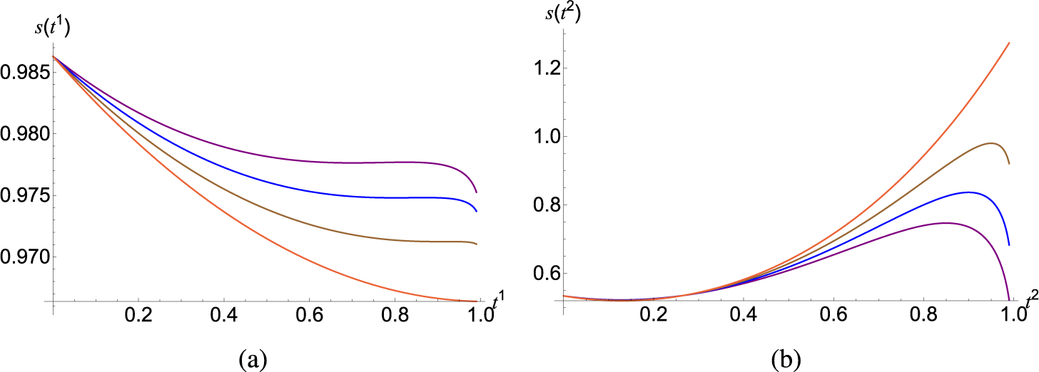


 Open access