


1 Introduction
Differential equations involving convection, diffusion and reaction are ubiquitous in various physical and engineering applications. Since a standard finite element method does not provide a stable approximation, as it yields a spurious approximate solution, a stabilization technique should be used. There are a wide range of stabilization techniques for advection-dominated problems [Reference Becker and Braack1, Reference Braack and Burman3, Reference Matthies, Skrzypacz and Tobiska21, Reference Roos, Stynes and Tobiska24].
The main reason for such a behaviour is the presence of interior or boundary layers in the solution. These boundary layers cause high gradients of the solution in the neighbourhood of the layers. A wide range of stabilization methods have been proposed to deal with these spurious modes caused by the boundary layers. Some popular methods are streamline-diffusion methods, least squares methods, residual-free bubbles, local projection schemes, continuous interior penalty methods and discontinuous Galerkin methods [Reference Johnson13, Reference Roos, Stynes and Tobiska24]. As there is a vast amount of literature on these stabilization approaches, we only focus on a few articles on the local projection stabilization approach which are relevant to our current work.
The local projection stabilization approach [Reference Ganesan and Tobiska10, Reference Knobloch and Tobiska16, Reference Matthies, Skrzypacz and Tobiska21, Reference Roos, Stynes and Tobiska24] is one of the most popular stabilization techniques for convection-dominated convection–diffusion–reaction problems with boundary or interior layers. There are mainly two forms of the local projection stabilization approach in the literature. One approach enriches the solution space by using bubble functions and another approach uses two different finite element grids to preserve the locality of the stabilization term [Reference Knobloch and Lube15, Reference Matthies, Skrzypacz and Tobiska21]. Working with bubble functions, we need to increase an additional set of degrees of unknowns, whereas working with two finite element grids, the discretization stencil increases and hence the sparsity of the system matrix decreases. Thus, both approaches increase the computational cost.
We introduce a new local projection stabilization technique based on a biorthogonal system for convection-dominated convection–diffusion–reaction differential equations. Neither does our approach need to enrich the finite element space by bubble functions, nor do we need two different finite element grids to achieve the locality of the stabilization term. Since the projection is performed by using a biorthogonal system, the locality is achieved as the biorthogonality condition yields a diagonal matrix. A similar biorthogonal approach is applied to stabilize the Stokes problem [Reference Lamichhane and Shaw-Carmody19]. However, approximation properties of the biorthogonal system and the error analysis are different for the convection–diffusion–reaction problem compared with the Stokes problem.
Another newly proposed local projection stabilization scheme [Reference Biswas, Dond and Gudi2, Reference Dond and Gudi7] also does not require the bubble enrichment and two different grids, but our approach is easier to extend to a higher order case. Moreover, the application of the biorthogonal system to compute projection is more natural than the patch-wise local projection stabilization proposed in [Reference Biswas, Dond and Gudi2, Reference Dond and Gudi7].
Let $\Omega \subset \mathbb R^d$
,
$\Omega \subset \mathbb R^d$
, $d \in \{2,3\}$
, be a bounded domain with a polygonal or polyhedral boundary
$d \in \{2,3\}$
, be a bounded domain with a polygonal or polyhedral boundary $\partial \Omega $
, where the boundary
$\partial \Omega $
, where the boundary $\partial \Omega $
is divided into two disjoint parts
$\partial \Omega $
is divided into two disjoint parts $\Gamma _D$
and
$\Gamma _D$
and $\Gamma _N$
. We consider the convection–diffusion–reaction equation
$\Gamma _N$
. We consider the convection–diffusion–reaction equation
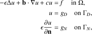 $$ \begin{align*} \begin{aligned} -\epsilon \Delta u + \mathbf{b} \cdot \nabla u + c u &= f \quad \, \text{in}\; \Omega, \\ u &= g_D \quad \text{on}\; \Gamma_D, \\ \epsilon \frac{\partial u}{\partial \mathbf n} &= g_N \quad \text{on}\; \Gamma_N, \end{aligned} \end{align*} $$
where $0<\epsilon \ll 1 $
is a constant, and
$0<\epsilon \ll 1 $
is a constant, and $\mathbf {b} \in [W^{1,\infty } (\Omega )]^d$
,
$\mathbf {b} \in [W^{1,\infty } (\Omega )]^d$
, $c \in L^{\infty }(\Omega )$
and
$c \in L^{\infty }(\Omega )$
and $f \in L^2(\Omega )$
are given functions satisfying
$f \in L^2(\Omega )$
are given functions satisfying
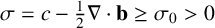 $$ \begin{align} \sigma = c- \tfrac{1}{2}\nabla\cdot \mathbf{b} \geq \sigma_0>0 \end{align} $$
for a constant $\sigma _0$
. Let
$\sigma _0$
. Let $ V_0 = \{v \in H^1(\Omega )\mid \, v|_{\Gamma _D} =0\}.$
The weak formulation of (1.1) is to find
$ V_0 = \{v \in H^1(\Omega )\mid \, v|_{\Gamma _D} =0\}.$
The weak formulation of (1.1) is to find $ u \in V_D=\{v \in H^1(\Omega )\mid v|_{\Gamma _D} =g_D\} $
such that
$ u \in V_D=\{v \in H^1(\Omega )\mid v|_{\Gamma _D} =g_D\} $
such that
 $$ \begin{align} a(u,v) =\ell(v), \quad v \in V_0, \end{align} $$
where
 $$ \begin{align*} a(u,v) =\epsilon\int_{\Omega} \nabla u\cdot \nabla v \,dx + \int_{\Omega} ( (\mathbf{b} \cdot \nabla u)\, v + c uv )\,dx , \quad \ell(v) =\int_{\Omega}fv\,dx + \int_{\Gamma_N} g_Nv\,ds. \end{align*} $$
Assuming that the inflow boundary is part of the Dirichlet boundary $\Gamma _D$
, that is,
$\Gamma _D$
, that is,
 $$ \begin{align} \{ x\in \partial \Omega \mid \mathbf{b}\cdot \mathbf n <0 \}\subset \Gamma_D, \end{align} $$
the condition in (1.1) guarantees the coercivity of the bilinear form $a(\cdot ,\cdot )$
on
$a(\cdot ,\cdot )$
on $V_0$
. Hence, the boundary value problem (1.2) has a unique solution in
$V_0$
. Hence, the boundary value problem (1.2) has a unique solution in $V_D$
by the Lax–Milgram lemma [Reference Brenner and Scott5, Reference Gilbarg and Trudinger11].
$V_D$
by the Lax–Milgram lemma [Reference Brenner and Scott5, Reference Gilbarg and Trudinger11].
The paper is organized as follows. In the next section, we present our finite element scheme. In Section 3, we prove that the formulation is well posed, and the finite element approximation satisfies optimal a priori error estimates. In Section 4, we introduce a posteriori error estimator that shows the direction of future works in the area of an adaptive finite element method. In Section 5, we present some numerical experiments to demonstrate the performance of our approach. Finally, we draw a conclusion in Section 6.
2 Finite element discretization
We consider a locally quasi-uniform shape regular triangulation $\mathcal {T}_h$
of the polygonal or polyhedral domain
$\mathcal {T}_h$
of the polygonal or polyhedral domain $\Omega $
, where
$\Omega $
, where $\mathcal {T}_h$
consists of d-simplices, convex quadrilaterals or hexahedra. Note that
$\mathcal {T}_h$
consists of d-simplices, convex quadrilaterals or hexahedra. Note that $\mathcal {T}_h$
denotes the set of elements, which are d-simplices, convex quadrilaterals or hexahedra. The diameter of an element
$\mathcal {T}_h$
denotes the set of elements, which are d-simplices, convex quadrilaterals or hexahedra. The diameter of an element $T \in \mathcal {T}_h$
is denoted by
$T \in \mathcal {T}_h$
is denoted by $h_T$
, and the mesh parameter h is the maximum diameter of all elements
$h_T$
, and the mesh parameter h is the maximum diameter of all elements $T \in \mathcal {T}_h$
.
$T \in \mathcal {T}_h$
.
Let $\hat {T}$
be a reference simplex or square or cube, where the reference simplex is defined as
$\hat {T}$
be a reference simplex or square or cube, where the reference simplex is defined as
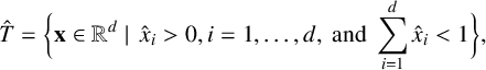 $$ \begin{align*} \hat{T}= \bigg\{ \mathbf{x} \in \mathbb R^d\mid\, \hat{x}_i>0, i=1,\ldots,d, \text{ and }\sum_{i=1}^d \hat{x}_i <1\bigg\},\end{align*} $$
and a reference square or cube $\hat {T}=(-1,1)^d$
. The finite element space is defined by the affine maps
$\hat {T}=(-1,1)^d$
. The finite element space is defined by the affine maps $F_T$
from a reference element
$F_T$
from a reference element $\hat {T}$
to a physical element
$\hat {T}$
to a physical element $T\in \mathcal {T}_h$
. Let
$T\in \mathcal {T}_h$
. Let $\mathcal {Q}_1(\hat {T})$
be the space of linear polynomials in
$\mathcal {Q}_1(\hat {T})$
be the space of linear polynomials in $\hat {T}$
in the variables
$\hat {T}$
in the variables $\hat {x}_1,\ldots , \hat {x}_d$
if
$\hat {x}_1,\ldots , \hat {x}_d$
if $\hat {T}$
is the reference simplex, and the space of bilinear or trilinear polynomials in
$\hat {T}$
is the reference simplex, and the space of bilinear or trilinear polynomials in $\hat T$
of
$\hat T$
of $\hat {x}_1,\ldots , \hat {x}_d$
if
$\hat {x}_1,\ldots , \hat {x}_d$
if $\hat T$
is the reference square or cube. Let
$\hat T$
is the reference square or cube. Let $F_T:\hat T \to T$
be the element mapping from the reference element
$F_T:\hat T \to T$
be the element mapping from the reference element $\hat T$
to a physical element
$\hat T$
to a physical element $T \in \mathcal {T}_h$
. This mapping is affine if T is a simplex, or T is a parallelotope. Then, the finite element space based on the mesh
$T \in \mathcal {T}_h$
. This mapping is affine if T is a simplex, or T is a parallelotope. Then, the finite element space based on the mesh $\mathcal {T}_h$
is defined as the space of continuous functions whose restrictions to an element T are obtained by the maps of given polynomial functions from the reference element [Reference Braess4–Reference Ciarlet6, Reference Quarteroni and Valli23]:
$\mathcal {T}_h$
is defined as the space of continuous functions whose restrictions to an element T are obtained by the maps of given polynomial functions from the reference element [Reference Braess4–Reference Ciarlet6, Reference Quarteroni and Valli23]:
 $$ \begin{align*} V_h= \{v_h \in H^1(\Omega)\mid v_h|_T=\hat{v}_h\circ F^{-1}_{T}, \hat{v}_h\in \mathcal{Q}_1(\hat{T}),\;T\in \mathcal{T}_h \},\quad V_{0,h} = V_h \cap V_0. \end{align*} $$
Let $g_{D,h}$
be a finite element approximation of
$g_{D,h}$
be a finite element approximation of $g_D$
on
$g_D$
on $\Gamma _D$
, which will be discussed later. The Galerkin formulation of (1.2) is to find
$\Gamma _D$
, which will be discussed later. The Galerkin formulation of (1.2) is to find $ u_h \in V_h$
with
$ u_h \in V_h$
with $u_h|_{\Gamma _D} = g_{D,h}$
such that
$u_h|_{\Gamma _D} = g_{D,h}$
such that
 $$ \begin{align} a(u_h,v_h)= \ell(v_h),\quad v_h \in V_{0,h}, \end{align} $$
where the bilinear form $a(\cdot ,\cdot )$
and the linear form
$a(\cdot ,\cdot )$
and the linear form $\ell (\cdot )$
are as defined in the last section. We say that convection dominates diffusion if
$\ell (\cdot )$
are as defined in the last section. We say that convection dominates diffusion if $\epsilon \ll \|\mathbf {b}\|_{L^{\infty }(\Omega )} h$
, and reaction dominates diffusion if
$\epsilon \ll \|\mathbf {b}\|_{L^{\infty }(\Omega )} h$
, and reaction dominates diffusion if $\epsilon \ll \sigma h^2$
. The Galerkin finite element approximation of (1.2) normally suffers from spurious oscillations if convection dominates diffusion, and/or reaction dominates diffusion [Reference Roos, Stynes and Tobiska24].
$\epsilon \ll \sigma h^2$
. The Galerkin finite element approximation of (1.2) normally suffers from spurious oscillations if convection dominates diffusion, and/or reaction dominates diffusion [Reference Roos, Stynes and Tobiska24].
2.1 A local projection stabilization
In this paper, we focus on analysing the finite element method based on the local projection stabilization approach using a biorthogonal system. The existing local projection stabilizations either use a two-level approach [Reference Becker and Braack1, Reference Braack and Burman3] or enrichment of the approximation space [Reference Matthies, Skrzypacz and Tobiska21]. The use of a biorthogonal system is motivated by these two observations of the existing stabilization. Working with a biorthogonal system, we neither need to use a two-level approach nor do we need to enrich the approximation space. In the following, we limit our discussion to the two-dimensional case, although an extension to the three-dimensional case is straightforward.
Let $\mathcal {B}_1=\{\varphi _1,\ldots ,\varphi _n\}$
be the set of finite element basis functions of
$\mathcal {B}_1=\{\varphi _1,\ldots ,\varphi _n\}$
be the set of finite element basis functions of $V_h$
with respect to the mesh
$V_h$
with respect to the mesh $\mathcal {T}_h$
. We now construct another set
$\mathcal {T}_h$
. We now construct another set $\mathcal {B}_2=\{\xi _1,\ldots ,\xi _n\} \subset L^2(\Omega )$
, which is biorthogonal to
$\mathcal {B}_2=\{\xi _1,\ldots ,\xi _n\} \subset L^2(\Omega )$
, which is biorthogonal to $\mathcal {B}_1$
, so that elements of
$\mathcal {B}_1$
, so that elements of $\mathcal {B}_1$
and
$\mathcal {B}_1$
and $\mathcal {B}_2$
satisfy a condition of the biorthogonality relation
$\mathcal {B}_2$
satisfy a condition of the biorthogonality relation
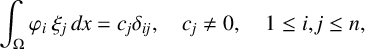 $$ \begin{align*} \int_{\Omega} \varphi_i \ \xi_j \, dx = c_j \delta_{ij}, \quad c_j\neq 0,\quad 1\le i,j \le n, \end{align*} $$
where $\delta _{ij}$
is the Kronecker symbol, and
$\delta _{ij}$
is the Kronecker symbol, and $c_j$
a scaling factor. This scaling factor
$c_j$
a scaling factor. This scaling factor $c_j$
can be chosen as proportional to the area
$c_j$
can be chosen as proportional to the area $|\text {supp} \xi _j|$
. We define another finite element space
$|\text {supp} \xi _j|$
. We define another finite element space
 $$ \begin{align*} Q_h=\text{span}\{\mathcal{B}_2\},\end{align*} $$
and assume that the space $Q_h$
has the approximation property
$Q_h$
has the approximation property
 $$ \begin{align*} \inf_{\mu_h \in Q_h} \|\mu - \mu_h \|_{0,\Omega} \leq h \|\mu\|_{1,\Omega},\quad \mu \in H^{1}(\Omega).\end{align*} $$
The basis functions $\{\xi _1,\ldots ,\xi _n\}$
are constructed in a reference element, and they are mapped to physical elements using a suitable affine transformation and combined together to construct the global basis functions of
$\{\xi _1,\ldots ,\xi _n\}$
are constructed in a reference element, and they are mapped to physical elements using a suitable affine transformation and combined together to construct the global basis functions of $Q_h$
in the same way as the global finite element basis functions of
$Q_h$
in the same way as the global finite element basis functions of $V_h$
are constructed. Here, we give the construction for a reference triangle. Let
$V_h$
are constructed. Here, we give the construction for a reference triangle. Let
 $$ \begin{align*} \hat T= \{ (\hat{x},\hat{y}) \in \mathbb R^2\mid\,\hat{x}>0,\hat{y}>0, \hat{x}+\hat{y}<1\}\end{align*} $$
be a reference triangle. The standard linear finite element basis functions for the reference triangle are defined as
 $$ \begin{align*} \hat \varphi_1=1-\hat{x}-\hat{y},\quad \hat\varphi_2=\hat{x}\quad \text{and}\quad \hat\varphi_3=\hat{y}, \end{align*} $$
associated with the three vertices $(0,0)$
,
$(0,0)$
, $(1,0)$
and
$(1,0)$
and $(0,1)$
, respectively.
$(0,1)$
, respectively.
Then the basis functions $\{\hat \xi _1,\,\hat \xi _2,\,\hat \xi _3\}$
, defined as
$\{\hat \xi _1,\,\hat \xi _2,\,\hat \xi _3\}$
, defined as
 $$ \begin{align*} \hat \xi_1=3-4\hat{x}-4\hat{y},\quad \hat\xi_2=4\hat{x}-1\quad \text{and}\quad \hat\xi_3=4\hat{y}-1, \end{align*} $$
satisfy the biorthogonality relationship with the basis functions $\{\hat \varphi _1,\hat \varphi _2,\hat \varphi _3\}$
with respect to the standard
$\{\hat \varphi _1,\hat \varphi _2,\hat \varphi _3\}$
with respect to the standard $L^2$
-inner product. We refer to the papers [Reference Lamichhane17, Reference Lamichhane18, Reference Lamichhane and Stephan20] for the construction of such a biorthogonal system for different finite element spaces.
$L^2$
-inner product. We refer to the papers [Reference Lamichhane17, Reference Lamichhane18, Reference Lamichhane and Stephan20] for the construction of such a biorthogonal system for different finite element spaces.
For the finite element convergence, we introduce the following two quasi-projection operators: $\Pi _h:L^2(\Omega )\rightarrow V_h$
and
$\Pi _h:L^2(\Omega )\rightarrow V_h$
and $\Pi ^*_h:L^2(\Omega )\rightarrow Q_h$
defined by
$\Pi ^*_h:L^2(\Omega )\rightarrow Q_h$
defined by
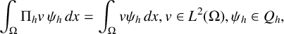 $$ \begin{align*} \int_{\Omega} \Pi_hv\, \psi_h \,dx = \int_{\Omega} v \psi_h \,dx, v \in L^2(\Omega), \psi_h \in Q_h, \end{align*} $$
and
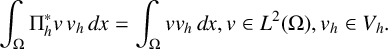 $$ \begin{align*} \int_{\Omega} \Pi^*_hv\, v_h \,dx = \int_{\Omega} v v_h \,dx, v \in L^2(\Omega), v_h \in V_h. \end{align*} $$
In the following, we use a generic constant C, which will take different values at different places but always will be independent of the mesh-size h. For an element $K\in \mathcal {T}_h$
, let
$K\in \mathcal {T}_h$
, let $\omega (K)$
be the union of support of all basis functions associated with K, and
$\omega (K)$
be the union of support of all basis functions associated with K, and $h_{\omega (K)}$
be the local mesh-size associated with
$h_{\omega (K)}$
be the local mesh-size associated with $\omega (K)$
. Hence,
$\omega (K)$
. Hence, $h_K \leq h_{\omega (K)}$
, where
$h_K \leq h_{\omega (K)}$
, where $h_K$
is the mesh-size of the element K. We now list some main properties of
$h_K$
is the mesh-size of the element K. We now list some main properties of $\Pi _h$
in the following lemma. We refer to the work of Kim et al. [Reference Kim, Lazarov, Pasciak and Vassilevski14] and Lamichhane [Reference Lamichhane17] for a proof of this lemma, where
$\Pi _h$
in the following lemma. We refer to the work of Kim et al. [Reference Kim, Lazarov, Pasciak and Vassilevski14] and Lamichhane [Reference Lamichhane17] for a proof of this lemma, where $\Pi _h$
is introduced as the mortar projection operator.
$\Pi _h$
is introduced as the mortar projection operator.
Lemma 2.1. Let $K\in \mathcal {T}_h$
. Here,
$K\in \mathcal {T}_h$
. Here, $\Pi _h$
and
$\Pi _h$
and $\Pi ^*_h$
have the following properties.
$\Pi ^*_h$
have the following properties.
-
(1) Stability in $L^2$
-norm:
$$ \begin{align*} \|\Pi_h v\|_{0,K}\leq C \|v\|_{0,\omega(K)},\quad \|\Pi^*_h v\|_{0,K}\leq C \|v\|_{0,\omega(K)},\quad v \in L^2(\omega(K)), \end{align*} $$
$L^2$
-norm:
$$ \begin{align*} \|\Pi_h v\|_{0,K}\leq C \|v\|_{0,\omega(K)},\quad \|\Pi^*_h v\|_{0,K}\leq C \|v\|_{0,\omega(K)},\quad v \in L^2(\omega(K)), \end{align*} $$
and
$$\begin{align*}\|\Pi_h v\|_{0,\Omega}\leq C \|v\|_{0,\Omega},\quad \|\Pi^*_h v\|_{0,\Omega}\leq C \|v\|_{0,\Omega}, \quad v \in L^2(\Omega). \end{align*}$$
-
(2) Stability in
$H^1$
-norm:
$$ \begin{align*} |\Pi_h v|_{1,K} \leq C|v|_{1,\omega(K)}, \quad v \in H^1(\omega(K)) \quad\text{and} \quad |\Pi_h v|_{1,\Omega} \leq C|v|_{1,\Omega}, \quad v \in H^1(\Omega). \end{align*} $$
-
(3) Approximation in
$L^2$
-norm: if
$ v \in H^{2}(\omega (K))$
and
$w \in H^{1}(\omega (K))$
for
$ K \in \mathcal {T}_h$
,
$$ \begin{align*} \|\Pi_h v-v\|_{0,K} \leq Ch^2 \|v\|_{2,\omega(K)}\quad\text{and}\quad \|\Pi^*_h w-w\|_{0,K}\leq C h \|w\|_{1,\omega(K)}. \end{align*} $$
Thus, for
$ v \in H^{2}(\Omega )$
and
$ w \in H^{1}(\Omega )$
,
$$ \begin{align*} \|\Pi_h v-v\|_{0,\Omega} \leq Ch^{2} \|v\|_{2,\Omega}\quad\text{and}\quad \|\Pi^*_h w-w\|_{0,\Omega}\leq C h \|w\|_{1,\Omega}. \end{align*} $$
-
(4) Approximation in
$H^1$
-norm: if
$ v \in H^{2}(\omega (K))$
, for
$ K \in \mathcal {T}_h$
,
$$ \begin{align*} \|\Pi_h v-v\|_{1,K} \leq Ch \|v\|_{2,\omega(K)}. \end{align*} $$
Thus, for
$ v \in H^{2}(\Omega )$
,
$$ \begin{align*} \|\Pi_h v-v\|_{1,\Omega} \leq Ch \|v\|_{2,\Omega}. \end{align*} $$


We now introduce the stabilization of the Galerkin finite element equation (2.1) using the fluctuation operator
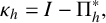 $$ \begin{align*} \kappa_h = I - \Pi^*_h, \end{align*} $$
where $I:L^2(\Omega ) \to L^2(\Omega ) $
is the identity operator. Adding the stabilization term
$I:L^2(\Omega ) \to L^2(\Omega ) $
is the identity operator. Adding the stabilization term
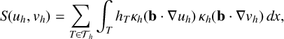
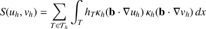 $$ \begin{align*} S(u_h,v_h) = \sum_{T \in \mathcal{T}_h} \int_{T} h_T \kappa_h (\mathbf{b}\cdot \nabla u_h)\, \kappa_h (\mathbf{b}\cdot \nabla v_h)\, dx \end{align*} $$
to the Galerkin formulation of the problem, we arrive at the problem of finding $ u_h \in V_h$
with
$ u_h \in V_h$
with $u_h|_{\Gamma _D} = g_{D,h}$
such that
$u_h|_{\Gamma _D} = g_{D,h}$
such that
 $$ \begin{align*} \epsilon\int_{\Omega} \nabla u_h\cdot \nabla v_h \,dx + \int_{\Omega} ( (\mathbf{b} \cdot \nabla u_h)+ c u_h )v_h \,dx +S(u_h,v_h) =\ell(v_h), \; v_h \in V_{0,h}. \end{align*} $$
Defining the bilinear form $A(\cdot ,\cdot )$
by
$A(\cdot ,\cdot )$
by
 $$ \begin{align*} A(u_h,v_h) = \epsilon\int_{\Omega} \nabla u_h\cdot \nabla v_h \,dx + \int_{\Omega} ( (\mathbf{b} \cdot \nabla u_h) + c u_h ) v_h \,dx +S(u_h,v_h), \end{align*} $$
our problem is to find $ u_h \in V_h$
with
$ u_h \in V_h$
with $u_h|_{\Gamma _D} = g_{D,h}$
such that
$u_h|_{\Gamma _D} = g_{D,h}$
such that
 $$ \begin{align} A(u_h,v_h)=\ell(v_h),\; v_h \in V_{0,h}. \end{align} $$
3 A priori error estimate
We perform the error analysis using the following mesh-dependent norm for $v_h \in V_h$
:
$v_h \in V_h$
:
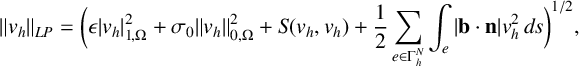 $$ \begin{align*} \|v_h\|_{LP} =\bigg(\epsilon |v_h|_{1,\Omega}^2+ \sigma_0 \|v_h\|_{0,\Omega}^2+S(v_h,v_h)+ \frac{1}{2} \sum_{e \in \Gamma^N_h} \int_{e} |\mathbf{b}\cdot\mathbf n|v_h^2\,ds \bigg)^{1/2}, \end{align*} $$
where $\Gamma ^N_h$
is the set of all edges on the boundary
$\Gamma ^N_h$
is the set of all edges on the boundary $\Gamma _N$
of
$\Gamma _N$
of $\Omega $
. With suitable approximation properties of the local projection, the error analysis is similar to the error analysis of the standard local projection stabilization approach [Reference Matthies, Skrzypacz and Tobiska21]. For simplicity, we let
$\Omega $
. With suitable approximation properties of the local projection, the error analysis is similar to the error analysis of the standard local projection stabilization approach [Reference Matthies, Skrzypacz and Tobiska21]. For simplicity, we let
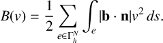 $$ \begin{align*} B(v) = \frac{1}{2} \sum_{e \in \Gamma^N_h} \int_{e} |\mathbf{b}\cdot\mathbf n|v^2\,ds. \end{align*} $$
The coercivity of the bilinear form $A(\cdot ,\cdot )$
with respect to the norm
$A(\cdot ,\cdot )$
with respect to the norm $\|\cdot \|_{LP}$
follows by using conditions (1.1) and (1.3). We refer to the work of Matthies et al. [Reference Matthies, Skrzypacz and Tobiska21] for a proof of the following lemma.
$\|\cdot \|_{LP}$
follows by using conditions (1.1) and (1.3). We refer to the work of Matthies et al. [Reference Matthies, Skrzypacz and Tobiska21] for a proof of the following lemma.
Lemma 3.1. There exists a constant $C>0$
independent of the mesh-size h such that
$C>0$
independent of the mesh-size h such that
 $$ \begin{align*} A(v_h,v_h) \geq C \|v_h\|^2_{LP},\quad v_h \in V_{0,h}.\end{align*} $$
The estimate for the consistency error is given in the next lemma.
Lemma 3.2. Let $u \in H^{k+1}(\Omega )$
and
$u \in H^{k+1}(\Omega )$
and $u_h \in V_h$
be the solutions of (1.2) and (2.2), respectively. Then,
$u_h \in V_h$
be the solutions of (1.2) and (2.2), respectively. Then,
 $$ \begin{align*} A(u-u_h, w_h) = S(u , w_h), \quad w_h \in V_{h,0}.\end{align*} $$
Moreover,
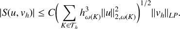 $$ \begin{align*} |S(u,v_h)| \leq C \bigg(\sum_{K \in \mathcal{T}_h} h_{\omega(K)}^{3}\|u\|_{2,\omega(K)}^2\bigg)^{1/2} \|v_h\|_{LP}.\end{align*} $$
Proof. From (1.2), we get for $w_h \in V_{0,h}$
,
$w_h \in V_{0,h}$
,
 $$ \begin{align*} \epsilon\int_{\Omega} \nabla u\cdot \nabla w_h \,dx + \int_{\Omega} [ (\mathbf{b} \cdot \nabla u)+ c u ]w_h\,dx =\int_{\Omega}fw_h\,dx + \int_{\Gamma_N} g_Nw_h\,ds. \end{align*} $$
Subtracting (2.2) from this equation, we obtain
 $$ \begin{align*} \epsilon\int_{\Omega} \nabla (u-u_h)\cdot \nabla w_h \,dx + \int_{\Omega} [ (\mathbf{b} \cdot \nabla (u-u_h)) + c (u-u_h) ]w_h\,dx +S(u_h,w_h) = 0. \end{align*} $$
The first equation now follows by using the definition of $A(\cdot ,\cdot )$
. Applying the Cauchy–Schwarz inequality to
$A(\cdot ,\cdot )$
. Applying the Cauchy–Schwarz inequality to
 $$ \begin{align*} S(u_h,v_h) = \sum_{T \in \mathcal{T}_h} \int_{T} h_T \kappa_h (\mathbf{b}\cdot \nabla u_h)\, \kappa_h (\mathbf{b}\cdot \nabla v_h)\, dx,\end{align*} $$
we obtain
 $$ \begin{align*} |S(u,v_h) | \leq \sqrt{S(u,u)} \sqrt{S(v_h,v_h)}.\end{align*} $$
Now we use the approximation property of $\Pi ^*_h$
and the fact that
$\Pi ^*_h$
and the fact that $\mathbf {b} \in [W^{1,\infty } (\Omega )]^d$
to obtain the result
$\mathbf {b} \in [W^{1,\infty } (\Omega )]^d$
to obtain the result
 $$ \begin{align*} |S(u,v_h)| \leq C \bigg(\sum_{K \in \mathcal{T}_h} h_{\omega(K)}^{3}\|u\|_{2,\omega(K)}^2\bigg)^{1/2} \|v_h\|_{LP}\,.\\[-45pt] \end{align*} $$
The following approximation property holds for the projected function $\Pi _hu$
in the
$\Pi _hu$
in the $LP$
-norm.
$LP$
-norm.
Lemma 3.3. We have the following estimate for $u \in H^{2}(\Omega )$
:
$u \in H^{2}(\Omega )$
:
 $$ \begin{align*} \|u - \Pi_hu\|_{LP} \leq C \bigg(\sum_{K \in \mathcal{T}_h} (\epsilon+\sigma_0 h^2_{\omega(K)}+h_{\omega(K)}) h_{\omega(K)}^{2}\|u\|_{2,\omega(K)}^2\bigg)^{1/2}.\end{align*} $$
Proof. First, we note that
 $$ \begin{align*} \|u-\Pi_h u \|_{LP} &=(\epsilon |u-\Pi_h u |_{1,\Omega}^2+ \sigma_0 \|u-\Pi_h u \|_{0,\Omega}^2 \nonumber \\ &\quad +S(u-\Pi_h u ,u-\Pi_h u )+ B(u-\Pi_hu))^{1/2}. \end{align*} $$
Let $e \subset K$
be an edge of a triangle or quadrilateral
$e \subset K$
be an edge of a triangle or quadrilateral $K \in \mathcal {T}_h$
. Using the following trace estimate:
$K \in \mathcal {T}_h$
. Using the following trace estimate:
 $$ \begin{align*} \|v\|_{0,e} \leq C [h_K^{1/2} |v|_{1,K} + h_K^{-1/2} \|v\|_{0,K}],\end{align*} $$
we get
 $$ \begin{align*} \|u-\Pi_hu\|_{0,e} \leq C [h_K^{1/2}|u-\Pi_hu|_{1,K} + h_K^{-1/2}\|u-\Pi_hu\|_{0,K}].\end{align*} $$
We use the approximation property of $\Pi _h$
to get
$\Pi _h$
to get
 $$ \begin{align} \|u-\Pi_hu\|_{0,e} \leq C h_{\omega(K)}^{3/2} \|u\|_{2,\omega(K)}. \end{align} $$
Hence,
 $$ \begin{align*} B(u - \Pi_hu) &= \frac{1}{2} \sum_{e \in \Gamma^N_h} \int_{e} |\mathbf{b}\cdot\mathbf n| (u-\Pi_hu)^2\,ds\\ &\leq C \sum_{e \in \Gamma^N_h} \|u-\Pi_hu\|^2_{0,e} \leq C \sum_{K \in \mathcal{T}_h} h_{\omega(K)}^{3} \|u\|^2_{2,\omega(K)}.\end{align*} $$
We now consider the stabilization term in the estimate
 $$ \begin{align*} S(u-\Pi_hu, u - \Pi_hu) = \sum_{T \in \mathcal{T}_h} \int_{T} h_T (\kappa_h (\mathbf{b}\cdot \nabla (u-\Pi_h u)^2\, dx.\end{align*} $$
Using the $L^2$
-stability of
$L^2$
-stability of $\Pi ^*_h$
and the approximation property of
$\Pi ^*_h$
and the approximation property of $\Pi _h$
combined with the fact that
$\Pi _h$
combined with the fact that $\mathbf {b} \in [W^{1,\infty } (\Omega )]^d$
, we get
$\mathbf {b} \in [W^{1,\infty } (\Omega )]^d$
, we get
 $$ \begin{align*} S(u-\Pi_hu, u - \Pi_hu) \leq 2 \sum_{T \in \mathcal{T}_h} h_T\|\mathbf{b}\cdot \nabla (u-\Pi_h u\|_{0,T}^2 \leq 2 \sum_{T \in \mathcal{T}_h} h_{\omega(T)}^3 \|u\|^2_{2,\omega(T)} .\\[-45pt] \end{align*} $$
Lemma 3.4. Let $u \in H^{2}(\Omega )$
. Then for
$u \in H^{2}(\Omega )$
. Then for $v_h \in V_{h,0}$
, we have
$v_h \in V_{h,0}$
, we have
 $$ \begin{align*} |S(\Pi_hu-u,v_h)| \leq C \bigg(\sum_{K \in \mathcal{T}_h} h_{\omega(K)}^{3}\|u\|_{2,\omega(K)}^2\bigg)^{1/2} \|v_h\|_{LP}.\end{align*} $$
Proof. We start with the Cauchy–Schwarz inequality to write
 $$ \begin{align*} |S(\Pi_hu-u,v_h)| \leq S(\Pi_hu-u,\Pi_hu-u)^{1/2} S(v_h,v_h)^{1/2}.\end{align*} $$
The rest of the proof follows as in the last part of Lemma 3.3.
Theorem 3.5. Let $u \in H^{2}(\Omega )$
and
$u \in H^{2}(\Omega )$
and $u_h \in V_h$
be the solutions of (1.2) and (2.2), respectively. Then there exists a constant C independent of the mesh-size h such that the following a priori error estimate holds:
$u_h \in V_h$
be the solutions of (1.2) and (2.2), respectively. Then there exists a constant C independent of the mesh-size h such that the following a priori error estimate holds:
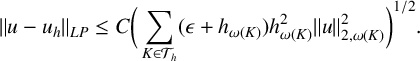 $$ \begin{align*} \|u - u_h\|_{LP} \leq C \bigg(\sum_{K \in \mathcal{T}_h} (\epsilon+ h_{\omega(K)}) h_{\omega(K)}^{2}\|u\|_{2,\omega(K)}^2\bigg)^{1/2}.\end{align*} $$
Proof. We first use the triangle inequality to write
 $$ \begin{align} \|u-u_h\|_{LP} \leq \|u-\Pi_hu\|_{LP} + \|\Pi_h u -u_h\|_{LP}. \end{align} $$
The approximation of the first term on the right-hand side of (3.2) is given in Lemma 3.3. We now turn our attention on estimating the second term on the right-hand side of (3.2). We first use the coercivity of $A(\cdot ,\cdot )$
to write
$A(\cdot ,\cdot )$
to write
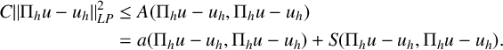 $$ \begin{align*} C \|\Pi_h u - u_h\|_{LP}^2 &\leq A(\Pi_h u - u_h, \Pi_h u - u_h) \\ &= a(\Pi_h u - u_h, \Pi_h u - u_h) + S(\Pi_h u - u_h, \Pi_h u - u_h). \end{align*} $$
For brevity, we let $w_h = \Pi _h u - u_h.$
Then,
$w_h = \Pi _h u - u_h.$
Then,
 $$ \begin{align*} C \|\Pi_h u - u_h\|_{LP}^2 \leq a(\Pi_h u - u, w_h) + a(u - u_h, w_h) + S(\Pi_h u - u, w_h) + S(u - u_h, w_h). \end{align*} $$
From Lemma 3.2, we have
 $$ \begin{align*}a(u - u_h, w_h) + S(u - u_h, w_h) = S(u,w_h),\end{align*} $$
and hence
 $$ \begin{align*} C \|\Pi_h u - u_h\|_{LP}^2 &\leq a(\Pi_h u - u, w_h) +S(\Pi_h u - u, w_h) + S(u , w_h). \end{align*} $$
We now let
 $$ \begin{align*} I_1 = a(\Pi_h u - u, w_h) , \; I_2= S(\Pi_h u - u, w_h) \quad \text{and}\quad I_3 = S(u,w_h),\end{align*} $$
so that
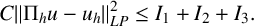 $$ \begin{align*} C \|\Pi_h u - u_h\|_{LP}^2 \leq I_1 + I_2 +I_3.\end{align*} $$
Since
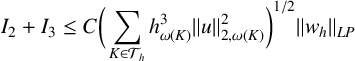 $$ \begin{align} I_2 + I_3 \leq C \bigg(\sum_{K \in \mathcal{T}_h} h_{\omega(K)}^{3}\|u\|_{2,\omega(K)}^2\bigg)^{1/2} \|w_h\|_{LP} \end{align} $$
from Lemmas 3.2 and 3.4, we need to estimate $I_1$
only. We have
$I_1$
only. We have
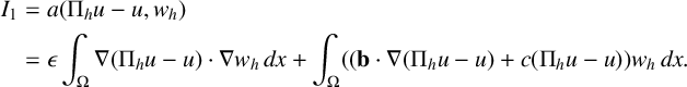 $$ \begin{align*} I_1&=a(\Pi_h u - u, w_h) \\ &= \epsilon\int_{\Omega} \nabla (\Pi_h u -u)\cdot \nabla w_h \,dx + \int_{\Omega} ( (\mathbf{b} \cdot \nabla (\Pi_hu -u)+ c (\Pi_h u -u) )w_h \,dx. \end{align*} $$
Thus, we have, from the approximation property of $\Pi _h$
,
$\Pi _h$
,
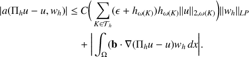 $$ \begin{align} \nonumber |a(\Pi_h u - u, w_h)| &\leq C \bigg(\sum_{K \in \mathcal{T}_h} (\epsilon +h_{\omega(K)} ) h_{\omega(K)} \|u\|_{2,\omega(K)} \bigg) \|w_h\|_{LP}\\ &\quad +\bigg| \int_{\Omega} (\mathbf{b} \cdot \nabla (\Pi_hu -u)w_h\,dx\bigg|. \end{align} $$
We integrate by parts the advection term and get
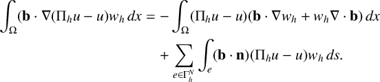 $$ \begin{align*} \int_{\Omega} (\mathbf{b} \cdot \nabla (\Pi_hu -u)w_h\,dx &= -\int_{\Omega} (\Pi_hu -u) (\mathbf{b} \cdot \nabla w_h +w_h \nabla \cdot \mathbf{b}) \,dx \\ &\quad + \sum_{e \in \Gamma^N_h} \int_{e} (\mathbf{b}\cdot\mathbf n) (\Pi_hu -u)w_h\,ds. \end{align*} $$
Let
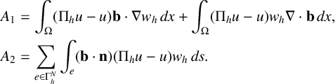 $$ \begin{align*} A_1 &= \int_{\Omega} (\Pi_hu -u) \mathbf{b} \cdot \nabla w_h\,dx +\int_{\Omega} (\Pi_hu -u) w_h \nabla \cdot \mathbf{b} \,dx , \\ A_2 &= \sum_{e \in \Gamma^N_h} \int_{e} (\mathbf{b}\cdot\mathbf n) (\Pi_hu -u)w_h\,ds. \end{align*} $$
We first consider the first term in $A_1$
. By using the definition of
$A_1$
. By using the definition of $\Pi _h$
, we have
$\Pi _h$
, we have
 $$ \begin{align*} \int_{\Omega} (\Pi_hu -u) \mathbf{b} \cdot \nabla w_h \,dx = \int_{\Omega} (\Pi_hu -u) \mathbf{b} \cdot \nabla w_h \,dx - \int_{\Omega} (\Pi_hu -u) \Pi^*_h(\mathbf{b} \cdot \nabla w_h) \,dx.\end{align*} $$
Thus, we get
 $$ \begin{align*} \int_{\Omega} (\Pi_hu -u) \mathbf{b} \cdot \nabla w_h \,dx &= \int_{\Omega} (\Pi_hu -u) \kappa_h( \mathbf{b} \cdot \nabla w_h) \,dx \\ &=\sum_{K \in \mathcal{T}_h} \int_{K} h_K^{-1/2} (\Pi_hu -u) h_K^{1/2}\kappa_h( \mathbf{b} \cdot \nabla w_h) \,dx. \end{align*} $$
Hence, an application of the approximation property of $\Pi _h$
yields
$\Pi _h$
yields
 $$ \begin{align*} \int_{\Omega} (\Pi_hu -u) \mathbf{b} \cdot \nabla w_h \,dx \leq C \sum_{K \in \mathcal{T}_h} h_{\omega(K)}^{3/2} \|u\|_{2, \omega(K)} \sqrt{ \sum_{K \in \mathcal{T}_h} \int_{K} h_{K} \kappa_h( \mathbf{b} \cdot \nabla w_h)^2\,dx}.\end{align*} $$
For the second term in $A_1$
, we use an approximation property of
$A_1$
, we use an approximation property of $\Pi _h$
to obtain
$\Pi _h$
to obtain
 $$ \begin{align*} \int_{\Omega} (\Pi_hu -u) w_h \nabla \cdot \mathbf{b} \,dx \leq C \sum_{K \in \mathcal{T}_h} h_{\omega(K)}^{2} \|u\|_{2, \omega(K)} \|w_h\|_{0,K}.\end{align*} $$
An application of the Cauchy–Schwarz inequality yields
 $$ \begin{align*} A_2= \sum_{e \in \Gamma^N_h} \int_{e} (\mathbf{b}\cdot\mathbf n) (\Pi_hu -u)w_h\,ds \leq C \sum_{e \in \Gamma^N_h} \||\mathbf{b}\cdot \mathbf n|^{1/2} (\Pi_h u -u)\|_{0,e} \||\mathbf{b}\cdot \mathbf n|^{1/2}w_h\|_{0,e}.\end{align*} $$
We now use the estimation (3.1) to write
 $$ \begin{align*} A_2 = \sum_{e \in \Gamma^N_h} \int_{e} (\mathbf{b}\cdot\mathbf n) (\Pi_hu -u)w_h\,ds \leq C \sum_{K \in \mathcal{T}_h}h_{\omega(K)}^{3/2} \|u\|_{2, \omega(K)} \|w_h\|_{LP}.\end{align*} $$
Combining the estimates for $A_1$
,
$A_1$
, $A_2$
and (3.4), we have
$A_2$
and (3.4), we have
 $$ \begin{align*}I_1 \leq |a(\Pi_h u - u, w_h)| \leq C \bigg(\sum_{K \in \mathcal{T}_h} [(\epsilon +h_{\omega(K)} ) h_{\omega(K)} +h_{\omega(K)}^{3/2}] \|u\|_{2, \omega(K)}\bigg)\|w_h\|_{LP}.\end{align*} $$
The proof now follows by using the estimate of $I_2+I_3$
from (3.3).
$I_2+I_3$
from (3.3).
3.1 Biquadratic finite element approach
We now briefly outline the biquadratic finite element approach using a biorthogonal system. The finite element space based on the mesh $\mathcal {T}_h$
is defined as
$\mathcal {T}_h$
is defined as
 $$ \begin{align*} W_h= \{v_h \in H^1(\Omega)\mid v_h|_T=\hat{v}_h\circ F^{-1}_{T}, \hat{v}_h\in \mathcal{Q}_2(\hat{T}), T\in \mathcal{T}_h \},\quad W_{0,h} = W_h \cap V_0, \end{align*} $$
where $\mathcal {Q}_2(\hat {T})$
is the space of the biquadratic finite element space on the element T. In this case, we need a better approximation property for the space
$\mathcal {Q}_2(\hat {T})$
is the space of the biquadratic finite element space on the element T. In this case, we need a better approximation property for the space $Q_h$
. While both projectors
$Q_h$
. While both projectors $\Pi _h$
and
$\Pi _h$
and $\Pi ^*_h$
are stable in
$\Pi ^*_h$
are stable in $L^2$
- and
$L^2$
- and $H^1$
-norms, they should satisfy the following properties.
$H^1$
-norms, they should satisfy the following properties.
-
(1) Approximation in
$L^2$
-norm: if
$ v \in H^{3}(\omega (K))$
and
$w \in H^{2}(\omega (K))$
for
$ K \in \mathcal {T}_h$
, then
$$ \begin{align*} \|\Pi_h v-v\|_{0,K} \leq Ch^3 \|v\|_{3,\omega(K)}\quad\text{and}\quad \|\Pi^*_h w-w\|_{0,K}\leq C h^2 \|w\|_{2,\omega(K)}. \end{align*} $$
Thus for
$ v \in H^{3}(\Omega )$
and
$ w \in H^{2}(\Omega )$
,
$$ \begin{align*} \|\Pi_h v-v\|_{0,\Omega} \leq Ch^{3} \|v\|_{3,\Omega}\quad\text{and}\quad \|\Pi^*_h w-w\|_{0,\Omega}\leq C h^2 \|w\|_{2,\Omega}. \end{align*} $$
-
(2) Approximation in
$H^1$
-norm: if
$ v \in H^{3}(\omega (K))$
for
$ K \in \mathcal {T}_h$
, then
$$ \begin{align*} \|\Pi_h v-v\|_{1,K} \leq Ch^2 \|v\|_{3,\omega(K)}. \end{align*} $$
Thus for
$ v \in H^{3}(\Omega )$
,
$$ \begin{align*} \|\Pi_h v-v\|_{1,\Omega} \leq Ch^2 \|v\|_{3,\Omega}. \end{align*} $$


As it is standard to have these approximation properties for $\Pi _h$
, approximation properties of
$\Pi _h$
, approximation properties of $\Pi _h^*$
follow from the fact that the space
$\Pi _h^*$
follow from the fact that the space $Q_h$
contains the bilinear finite element space [Reference Braess4, Reference Brenner and Scott5, Reference Lamichhane17]. Working with the biquadratic finite element method, we have the following approximation property of the discrete solution.
$Q_h$
contains the bilinear finite element space [Reference Braess4, Reference Brenner and Scott5, Reference Lamichhane17]. Working with the biquadratic finite element method, we have the following approximation property of the discrete solution.
Theorem 3.6. Let $u \in H^{3}(\Omega )$
and
$u \in H^{3}(\Omega )$
and $u_h \in W_h$
be the solutions of (1.2) and (2.2), respectively. Then, there exists a constant C independent of the mesh-size h such that the following a priori error estimate holds true:
$u_h \in W_h$
be the solutions of (1.2) and (2.2), respectively. Then, there exists a constant C independent of the mesh-size h such that the following a priori error estimate holds true:
 $$ \begin{align*} \|u - u_h\|_{LP} \leq C \bigg(\sum_{K \in \mathcal{T}_h} (\epsilon+ h_{\omega(K)}) h_{\omega(K)}^{4}\|u\|_{3,\omega(K)}^2\bigg)^{1/2}. \end{align*} $$
3.2 Weak boundary condition formulation
The formulation (1.2) uses the Dirichlet boundary as a strong condition. Imposing the Dirichlet boundary condition weakly is a way to alleviate the instability in the boundary layer [Reference Freund and Stenberg8]. We thus include the weak boundary condition using the Nitsche technique [Reference Freund and Stenberg8, Reference Heinrich and Nicaise12] in our stabilization method.
Let $\Gamma _{-} \subset \Gamma _{D}$
be defined as
$\Gamma _{-} \subset \Gamma _{D}$
be defined as $\Gamma _{-} = \lbrace x\in \Gamma _{D} \mid \boldsymbol {b}\cdot \boldsymbol {n} <0\rbrace $
and let
$\Gamma _{-} = \lbrace x\in \Gamma _{D} \mid \boldsymbol {b}\cdot \boldsymbol {n} <0\rbrace $
and let $\beta $
be a positive penalty parameter. We define the bilinear form
$\beta $
be a positive penalty parameter. We define the bilinear form $B_{w}( \cdot ,\cdot )$
and linear functional
$B_{w}( \cdot ,\cdot )$
and linear functional $F( \cdot )$
by
$F( \cdot )$
by
 $$ \begin{align*} B_{w}( u,v )&= -\langle \boldsymbol{b}\cdot \boldsymbol{n}u,v \rangle_{\Gamma_{-}} -\langle \varepsilon\nabla u\cdot\boldsymbol{n},v \rangle_{\Gamma_D} + \langle u,\varepsilon\nabla v\cdot\boldsymbol{n} \rangle_{\Gamma_D} + \beta \langle u,\varepsilon v \rangle_{-1,h,\Gamma_D},\\ F( v ) &= -\langle \boldsymbol{b}\cdot\boldsymbol{n}g,v \rangle_{\Gamma_{-}} + \langle g,\varepsilon\nabla v\cdot\boldsymbol{n} \rangle_{\Gamma_D} + \beta \langle g,\varepsilon v \rangle_{-1,h,\Gamma_D}, \end{align*} $$
where
 $$ \begin{align*} \langle u_{h},v_{h} \rangle_{\Gamma_D} &= \sum_{e\subset \Gamma_D} \int_{e} u_{h} v_{h} \; ds,\\ \langle u_{h},v_{h} \rangle_{-1,h,\Gamma_D} &= \sum_{e\subset \Gamma_D} h_{e}^{-1} \int_{e} u_{h} v_{h} \; ds. \end{align*} $$
This lets us reformulate the discrete problem to include the weak boundary condition as follows: find $u_{h} \in V_{h}$
such that
$u_{h} \in V_{h}$
such that
 $$ \begin{align*} \tilde{A}( u_{h},v_{h} ) = \tilde{\ell}( v_{h} ), \quad v_{h}\in V_{h}, \end{align*} $$
where
 $$ \begin{align*} \tilde{A}( u_{h},v_{h} ) &= A( u_{h},v_{h} ) + B_{w} ( u_{h},v_{h} ),\\ \tilde{\ell}( v_{h} ) &= \ell( v_{h} ) + F( v_{h} ). \end{align*} $$
The a priori error estimate presented in Theorem 3.6 extends easily to the formulation with the weak boundary condition [Reference Dond and Gudi7, Reference Freund and Stenberg8, Reference Heinrich and Nicaise12].
4 A posteriori error estimator
While not the main focus of this paper, we will briefly discuss a candidate for an a posteriori error estimator which can be used with the adaptive finite element method. When using an adaptive finite element scheme, an a posteriori error estimator and a marking scheme are used to determine which elements are to be refined at each iteration. The local error estimate
 $$ \begin{align} \eta_{T} ( \mathcal{T};v ) &= \bigg(h_{T}\int_{T} (\vec{b}\cdot \nabla v - \Pi_{h}^{*} {\vec{b}\cdot \nabla v})^{2} dx\bigg)^{1/2} \end{align} $$
is calculated for each element, and is used for calculating the global error estimator as well as selecting elements to be refined with the marking scheme. The global error estimator,
 $$ \begin{align} \eta ( \mathcal{T};v ) &= \bigg(\sum_{T\in \mathcal{T}} \eta_{T}( \mathcal{T};v )^{2}\bigg)^{1/2} \nonumber\\ &= \sqrt{S( v,v )}, \end{align} $$
is also used by the marking scheme. The Dörfler marking scheme is a popular marking scheme used in adaptive finite element which selects a set $\mathcal {M}$
, which is a subset of the collection of all elements
$\mathcal {M}$
, which is a subset of the collection of all elements $\mathcal {T}$
, such that the cardinality of
$\mathcal {T}$
, such that the cardinality of $\mathcal {M}$
is minimized, while also satisfying
$\mathcal {M}$
is minimized, while also satisfying
 $$ \begin{align} \theta \eta ( \mathcal{T};v )^{2} &\leq \sum_{T\in\mathcal{M}} \eta_{T}( \mathcal{T};v )^{2} \end{align} $$
for some user defined variable $\theta \in (0,1]$
. In other words, if any element is removed from
$\theta \in (0,1]$
. In other words, if any element is removed from $\mathcal {M}$
, then (4.3) would not be satisfied. Note that if
$\mathcal {M}$
, then (4.3) would not be satisfied. Note that if $\theta =0$
, then no elements are marked for refinement, and if
$\theta =0$
, then no elements are marked for refinement, and if $\theta =1$
, then all elements, except for those where
$\theta =1$
, then all elements, except for those where $\eta _{T}( \mathcal {T};v )=0$
, are marked for refinement, which is equivalent to using uniform refinement scheme.
$\eta _{T}( \mathcal {T};v )=0$
, are marked for refinement, which is equivalent to using uniform refinement scheme.
5 Numerical results
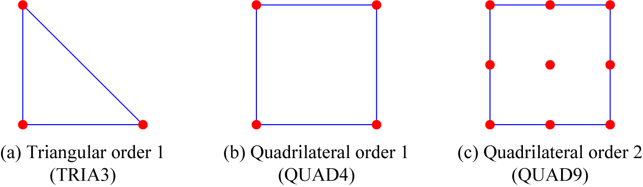
In this section, we present five examples, the first four of which act as numerical verification for the effectiveness of the stabilization method using our biorthogonal projection. The last example will demonstrate the ability of the stabilization method to be used in an adaptive finite element context. Examples 5.2, 5.3 and 5.4 are taken from [Reference Dond and Gudi7] and Example 5.5 is taken from [Reference Ganesan and Tobiska10]. For each example, we present the numerical convergence rates achieved when using the proposed stabilization on the standard linear triangular element, as well as the standard bilinear and biquadratic quadrilateral elements shown in Figure 1.
Remark 5.1. Working with general quadrilaterals, the reference element mapping $F_T$
is not affine. In the linear finite element method, this mapping can be approximated by an affine mapping by evaluating
$F_T$
is not affine. In the linear finite element method, this mapping can be approximated by an affine mapping by evaluating $F_T$
at the centroid of the element T.
$F_T$
at the centroid of the element T.
From this point onwards, we will refer to the standard linear triangular element as TRIA3, the standard bilinear quadrilateral element as QUAD4 and the standard biquadratic quadrilateral element as QUAD9.
The numerical results demonstrate the effectiveness of the biorthogonal stabilization method when using weak (Nitsche) boundary conditions, and also when using strong (Dirichlet) boundary conditions.
Example 5.2. We consider the partial differential equation (PDE) (1.1) with parameters $\varepsilon = 10^{-8}$
,
$\varepsilon = 10^{-8}$
, $\mathbf {b} = ( 2,3 )$
,
$\mathbf {b} = ( 2,3 )$
, $c=1$
, and where
$c=1$
, and where $\Omega = ( 0,1 )^{2}$
,
$\Omega = ( 0,1 )^{2}$
, $\Gamma _{D} = \partial \Omega $
,
$\Gamma _{D} = \partial \Omega $
, $\Gamma _{N} = \emptyset $
for which the exact solution is
$\Gamma _{N} = \emptyset $
for which the exact solution is
 $$ \begin{align*}u( x,y ) &= x^{3}( 1-x )y( 1-y^{4} ). \end{align*} $$
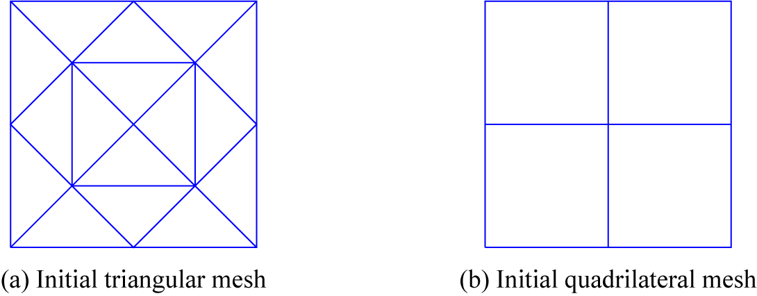
This problem, taken from [Reference Dond and Gudi7], has a smooth solution with no discontinuities on the domain, demonstrating how well the stabilization using the biorthogonal method works on simple problems. For the numerical testing, the initial mesh used for the triangular and quadrilateral elements are shown in Figure 2.
The standard elements, where the dots represent the degree of freedom points.
Initial mesh for Example 5.2.
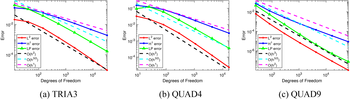
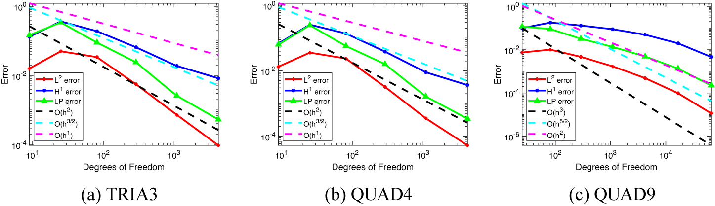
The norm error of the solutions generated by solving the weak boundary formulation achieve the expected rates of convergence. The three graphs in Figure 3 represent the solutions obtained using TRIA3, QUAD4 and QUAD9 elements. For each element, the $L^{2}$
,
$L^{2}$
, $H^{1}$
and
$H^{1}$
and $LP$
norms achieve or exceed the expected rate of convergence after the third iteration of the method.
$LP$
norms achieve or exceed the expected rate of convergence after the third iteration of the method.
The $L^{2}$
,
$L^{2}$
, $H^{1}$
and
$H^{1}$
and $LP$
error convergence using our method with the weak boundary condition formulation plotted against the number of degrees of freedom.
$LP$
error convergence using our method with the weak boundary condition formulation plotted against the number of degrees of freedom.
Example 5.3. This example considers the PDE (1.1) with coefficients $\varepsilon = 10^{-8}$
,
$\varepsilon = 10^{-8}$
, $\mathbf {b} = ( 1,1 )$
,
$\mathbf {b} = ( 1,1 )$
, $c=1$
, and where
$c=1$
, and where $\Omega = ( 0,1 )^{2}$
,
$\Omega = ( 0,1 )^{2}$
, $\Gamma _{D} = \partial \Omega $
,
$\Gamma _{D} = \partial \Omega $
, $\Gamma _{N} = \emptyset $
for which the exact solution is (see Figure 4a)
$\Gamma _{N} = \emptyset $
for which the exact solution is (see Figure 4a)
 $$ \begin{align*} u( x,y ) &= \bigg(\frac{\exp( (x-1)/\varepsilon )-1}{\exp( -1/\varepsilon )-1} + ( x-1 )\bigg) \bigg(\frac{\exp( (y-1)/\varepsilon )-1}{\exp( -1/\varepsilon )-1} + ( y-1 )\bigg). \end{align*} $$
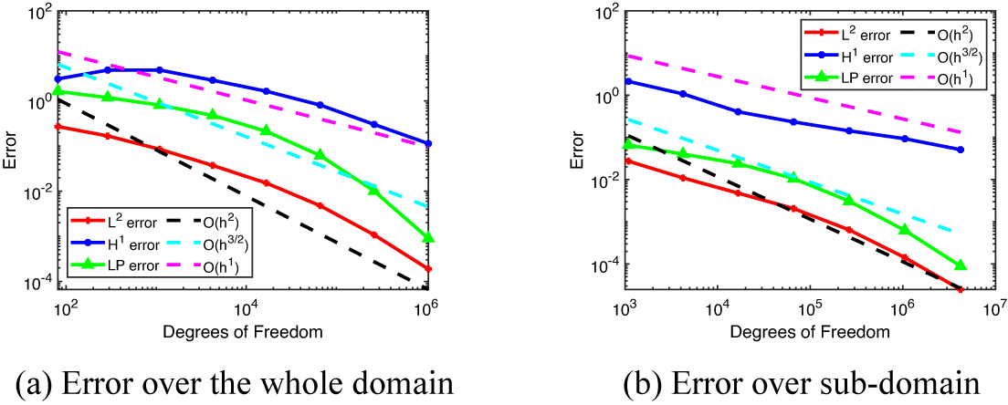
For this example from [Reference Dond and Gudi7], the error term of the solution taken over the entire domain is known to converge suboptimally for the $L^{2}$
and
$L^{2}$
and $H^{1}$
norms [Reference Dond and Gudi7, Reference Knobloch and Tobiska16, Reference Matthies and Tobiska22]. This is due to the exponential layer near the
$H^{1}$
norms [Reference Dond and Gudi7, Reference Knobloch and Tobiska16, Reference Matthies and Tobiska22]. This is due to the exponential layer near the $x=1$
and
$x=1$
and $y=1$
boundaries, where the layer is much smaller than the mesh size h. However, when the solution is analysed in a subdomain that does not contain the exponential layer, such as the subdomain
$y=1$
boundaries, where the layer is much smaller than the mesh size h. However, when the solution is analysed in a subdomain that does not contain the exponential layer, such as the subdomain $[ 0,3/4 ]^{2}$
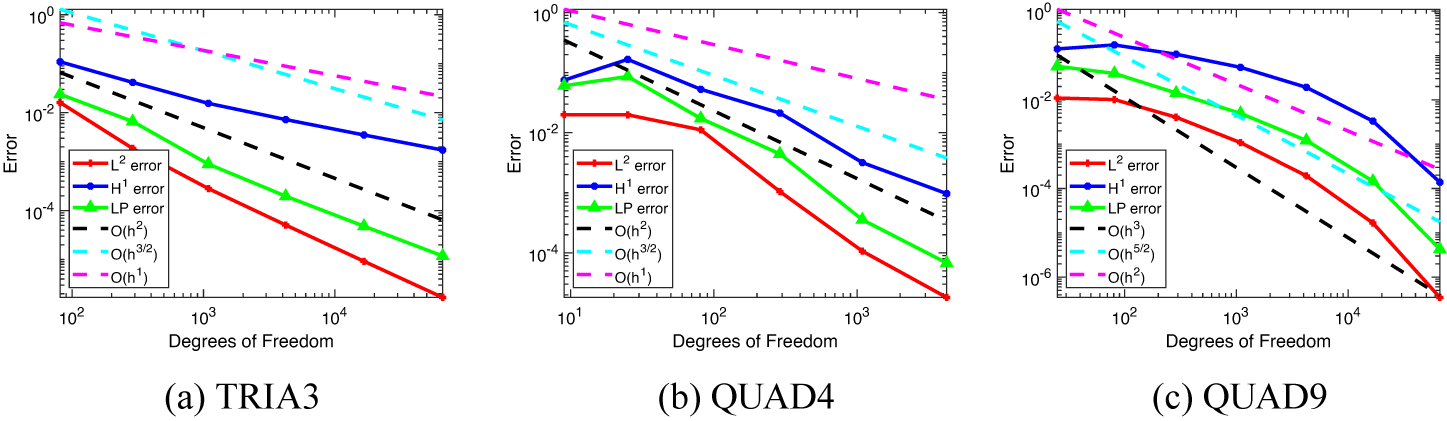
used in [Reference Knobloch and Tobiska16, Reference Matthies and Tobiska22], the approximation is as expected when using the biorthogonal stabilization with weak boundary condition. This is shown for all three element types in Figure 5.
$[ 0,3/4 ]^{2}$
used in [Reference Knobloch and Tobiska16, Reference Matthies and Tobiska22], the approximation is as expected when using the biorthogonal stabilization with weak boundary condition. This is shown for all three element types in Figure 5.
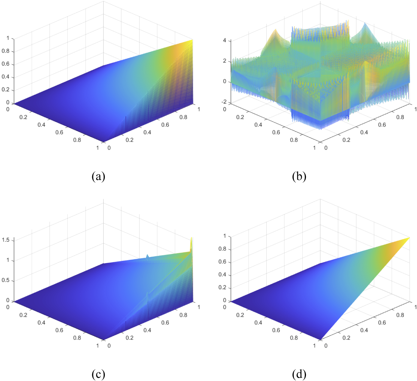
Linear finite element solutions generated for Example 5.3 with mesh size $h=0.0055$
. (a) Exact solution. (b) Solution using non-stabilized formulation. (c) Solution using stabilized formulation with strong boundary condition. (d) Stabilized formulation with weak boundary condition.
$h=0.0055$
. (a) Exact solution. (b) Solution using non-stabilized formulation. (c) Solution using stabilized formulation with strong boundary condition. (d) Stabilized formulation with weak boundary condition.
The $L^{2}$
,
$L^{2}$
, $H^{1}$
and
$H^{1}$
and $LP$
error convergence using our method with the weak boundary condition formulation over the subdomain
$LP$
error convergence using our method with the weak boundary condition formulation over the subdomain $[ 0,3/4 ]^{2}$
plotted against the number of degrees of freedom for Example 5.3.
$[ 0,3/4 ]^{2}$
plotted against the number of degrees of freedom for Example 5.3.
As displayed in Figure 4(b), if stabilization is not employed, the approximate solution has spurious oscillations. When stabilization is employed, the solutions improve vastly, as displayed in Figures 4(c) and 4(d), which employ stabilization with the strong and weak boundary conditions, respectively. This result is true not only for the TRIA3 case but also for the QUAD4 and QUAD9 elements.
Example 5.4. Here, we consider the PDE (1.1) with coefficients $\varepsilon = 10^{-8}$
,
$\varepsilon = 10^{-8}$
, $\mathbf {b} = ( 2,3 )$
,
$\mathbf {b} = ( 2,3 )$
, $c=2$
, and where
$c=2$
, and where $\Omega = ( 0,1 )^{2}$
,
$\Omega = ( 0,1 )^{2}$
, $\Gamma _{D} = \partial \Omega $
,
$\Gamma _{D} = \partial \Omega $
, $\Gamma _{N} = \emptyset $
for which the exact solution is
$\Gamma _{N} = \emptyset $
for which the exact solution is
 $$ \begin{align*} u( x,y ) &= 16x( 1-x )y( 1-y )\bigg( \frac{1}{2} + \frac{\tan^{-1}( 200( 1/4^{2} -( x-1/2 )^{2} -( y-1/2 )^{2} ) )}{\pi} \bigg). \end{align*} $$
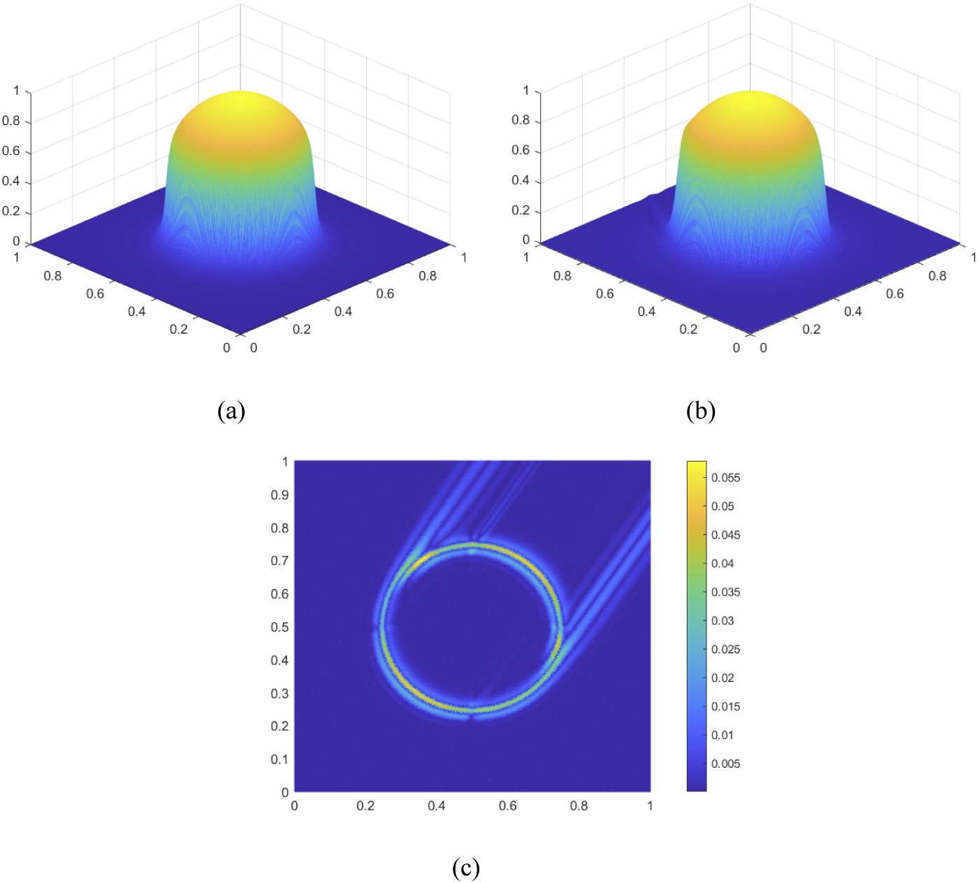
For this example from [Reference Dond and Gudi7], there is a transition layer imposed by the solution, much similar to that in Example 5.3. However, unlike Example 5.3, the transition layer is not located close to the boundary. In this problem, the transition layer lies on a circle in the domain with radius $0.25$
and centre
$0.25$
and centre $( 0.5,0.5 )$
. A different issue emerges than that in Example 5.3, since here the transition layer encompasses a large proportion of the domain.
$( 0.5,0.5 )$
. A different issue emerges than that in Example 5.3, since here the transition layer encompasses a large proportion of the domain.
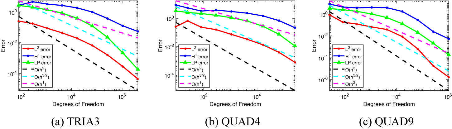
The results indicate that the transition layer causes the convergence rate to be below the theoretical expected rate in the early few steps of refinement, as shown in Figure 6. The discrepancy is eventually corrected when the mesh-size becomes smaller.
The $L^{2}$
,
$L^{2}$
, $H^{1}$
and
$H^{1}$
and $LP$
error convergence using our method with the weak boundary condition formulation plotted against the number of degrees of freedom for Example 5.4.
$LP$
error convergence using our method with the weak boundary condition formulation plotted against the number of degrees of freedom for Example 5.4.
The transition layer is the main source of error for the solutions generated, as shown in Figure 7. These graphs numerically demonstrate that most of the error occurs in the immediate neighbourhood of the transition layer.
Linear finite element solutions generated for Example 5.4 with mesh-size $h=0.0055$
. (a) Exact solution. (b) Stabilized formulation with weak boundary condition. (c) Magnitude of the error between exact solution and numerical solution with the weak boundary condition.
$h=0.0055$
. (a) Exact solution. (b) Stabilized formulation with weak boundary condition. (c) Magnitude of the error between exact solution and numerical solution with the weak boundary condition.
Example 5.5. In this example, we consider the PDE (1.1) with coefficients $\varepsilon = 10^{-8}$
,
$\varepsilon = 10^{-8}$
, $\mathbf {b} = ( 2,3 )$
,
$\mathbf {b} = ( 2,3 )$
, $c=1$
, and where
$c=1$
, and where $\Omega = ( 0,1 )^{2}$
,
$\Omega = ( 0,1 )^{2}$
, $\Gamma _{D} = \partial \Omega $
,
$\Gamma _{D} = \partial \Omega $
, $\Gamma _{N} = \emptyset $
for which the exact solution is
$\Gamma _{N} = \emptyset $
for which the exact solution is
 $$ \begin{align*} u( x,y ) &= xy^{2} - y^{2}\exp\bigg( \frac{2( x-1 )}{\varepsilon} \bigg) -x\exp\bigg( \frac{3( y-1 )}{\varepsilon} \bigg) + \exp\bigg( \frac{2( x-1 ) + 3( y-1 )}{\varepsilon} \bigg). \end{align*} $$
In this problem from [Reference Ganesan and Tobiska10], transition layers are again lying close to the $x=1$
and
$x=1$
and $y=1$
boundary. The error rates for this problem also perform poorly when taken to be over the entire domain for each respective element type. However, when evaluated over a subdomain that excludes the transition layers, the error rates perform as expected, which agrees with the observation made for the same phenomenon in Example 5.3. This is shown in Figure 8, where the expected rates of convergence are achieved or exceeded within the first iterations of the method for first-order elements and requires additional iterations for the second-order element.
$y=1$
boundary. The error rates for this problem also perform poorly when taken to be over the entire domain for each respective element type. However, when evaluated over a subdomain that excludes the transition layers, the error rates perform as expected, which agrees with the observation made for the same phenomenon in Example 5.3. This is shown in Figure 8, where the expected rates of convergence are achieved or exceeded within the first iterations of the method for first-order elements and requires additional iterations for the second-order element.
The $L^{2}$
,
$L^{2}$
, $H^{1}$
and
$H^{1}$
and $LP$
error convergence using our method with the weak boundary condition formulation over the subdomain
$LP$
error convergence using our method with the weak boundary condition formulation over the subdomain $[ 0,3/4 ]^{2}$
plotted against the number of degrees of freedom for Example 5.5.
$[ 0,3/4 ]^{2}$
plotted against the number of degrees of freedom for Example 5.5.
Example 5.6. To demonstrate how the stabilization performs with a non-constant convection term $\mathbf {b}$
, we consider the PDE (1.1) with coefficients
$\mathbf {b}$
, we consider the PDE (1.1) with coefficients $\varepsilon = 10^{-8}$
,
$\varepsilon = 10^{-8}$
, $\mathbf {b} = ( 1+x, 1+y )$
,
$\mathbf {b} = ( 1+x, 1+y )$
, $c=2$
, and where
$c=2$
, and where $\Omega = ( 0,1 )^{2}$
,
$\Omega = ( 0,1 )^{2}$
, $\Gamma _{D} = \partial \Omega $
,
$\Gamma _{D} = \partial \Omega $
, $\Gamma _{N} = \emptyset $
for which the exact solution is
$\Gamma _{N} = \emptyset $
for which the exact solution is
 $$ \begin{align*} u( x,y ) &= 16x( 1-x )y( 1-y )\bigg( \frac{1}{2} + \frac{\tan^{-1}( 200( 1/4^{2} -( x-1/2 )^{2} -( y-1/2 )^{2} ) )}{\pi} \bigg). \end{align*} $$
As noticed in Figure 9(a), the $L^2$
and
$L^2$
and $H^1$
errors converge with the orders of
$H^1$
errors converge with the orders of $O(h^{1.5})$
and
$O(h^{1.5})$
and $O( h )$
, respectively. The convergence rate for the
$O( h )$
, respectively. The convergence rate for the $LP$
errors are also noticed to achieve better than
$LP$
errors are also noticed to achieve better than $O(h^{1.5})$
convergence, which is consistent with the theory presented.
$O(h^{1.5})$
convergence, which is consistent with the theory presented. $L^{2}$
,
$L^{2}$
, $H^{1}$
and
$H^{1}$
and $LP$
error using TRIA3 element for Example 5.6, which has the non-constant
$LP$
error using TRIA3 element for Example 5.6, which has the non-constant $\mathbf {b}$
in the PDE formulation. (a) Graph presenting the errors over the entire domain. (b) Graph presenting the errors over the subdomain that does not include elements that cross the transition layer.
$\mathbf {b}$
in the PDE formulation. (a) Graph presenting the errors over the entire domain. (b) Graph presenting the errors over the subdomain that does not include elements that cross the transition layer.
The $L^{2}$
,
$L^{2}$
, $H^{1}$
and
$H^{1}$
and $LP$
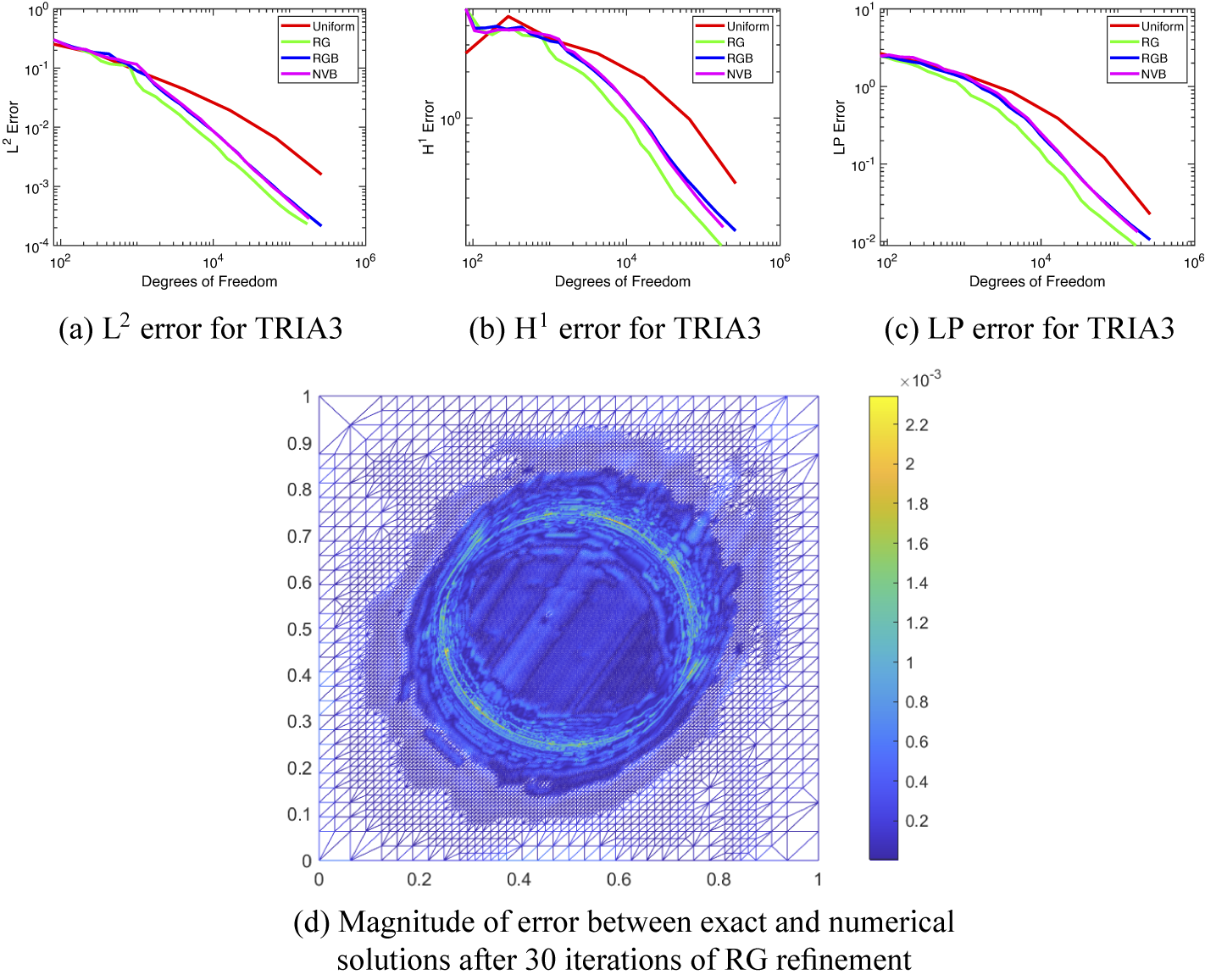
error convergence comparing the results from Example 5.4, denoted by the uniform refinement having the red line, with the adaptive finite element scheme using three different refinement schemes. The RG refinement is denoted by the green line, the RGB refinement is denoted by the blue line and the newest-vertex-bisection is denoted by the magenta line. The adaptive results are achieved using the Dörfler marking scheme with
$LP$
error convergence comparing the results from Example 5.4, denoted by the uniform refinement having the red line, with the adaptive finite element scheme using three different refinement schemes. The RG refinement is denoted by the green line, the RGB refinement is denoted by the blue line and the newest-vertex-bisection is denoted by the magenta line. The adaptive results are achieved using the Dörfler marking scheme with $\theta =0.5$
. (Colour available online.)
$\theta =0.5$
. (Colour available online.)
We now examine the errors in part of the domain $\Omega $
that does not include the transition layer. The results in Figure 9(b) demonstrate that the
$\Omega $
that does not include the transition layer. The results in Figure 9(b) demonstrate that the $L^2$
and
$L^2$
and $LP$
errors converge with order
$LP$
errors converge with order $O(h^{2})$
or better. The
$O(h^{2})$
or better. The $H^1$
error appears to converge slightly lower than
$H^1$
error appears to converge slightly lower than $O( h )$
.
$O( h )$
.
Example 5.7. For this example, we use the same problem presented in Example 5.4, except, here we extend the stabilization formulation to an adaptive finite element setting to demonstrate how the local stabilization term can be used to compute an a posteriori error estimator to reduce error. To this end, we use three standard refinement schemes, which are Red–Green (RG) refinement, Red–Green–Blue (RGB) refinement and newest-vertex-bisection (NVB) refinement on the TRIA3 elements [Reference Funken and Schmidt9]. The local a posteriori error estimator (4.1) is used with the Dörfler marking scheme (4.3), where $\theta =0.5$
, to select which elements to refine. The results in Figure 10 show that for all error measures used, the results presented in Example 5.4, denoted by the red line, can be further improved upon when the same stabilization term is used in conjunction with the adaptive finite element method. This is due to the marking scheme selecting the elements along the boundary layer for refinement, because they contribute a larger amount of the error as measured by the a posteriori error estimator (4.2).
$\theta =0.5$
, to select which elements to refine. The results in Figure 10 show that for all error measures used, the results presented in Example 5.4, denoted by the red line, can be further improved upon when the same stabilization term is used in conjunction with the adaptive finite element method. This is due to the marking scheme selecting the elements along the boundary layer for refinement, because they contribute a larger amount of the error as measured by the a posteriori error estimator (4.2).
This selection preference is revealed when comparing Figure 7(c), which shows the grid when using uniform refinement, with Figure 10(d), which uses RG adaptive refinement.
Example 5.8. The final example is the same problem presented in Example 5.4, however, this time, it is calculated on an unstructured grid. Here, we create an unstructured grid initially with random points, as shown in Figure 11(a), then use Red refinement on all elements to get the next refined grid for each iteration. This tests our stabilization method for an initial unstructured grid. From Figure 11(b), we see that the $L^{2}$
and
$L^{2}$
and $H^{1}$
convergence rates are of order
$H^{1}$
convergence rates are of order $O(h^{1.5})$
and
$O(h^{1.5})$
and $O( h )$
, respectively. The
$O( h )$
, respectively. The $LP$
error convergence rate also achieves the optimal rate of
$LP$
error convergence rate also achieves the optimal rate of $O(h^{1.5})$
as expected.
$O(h^{1.5})$
as expected.
The randomly generated unstructured grid and the error convergence when using the TRIA3 elements.

6 Conclusion
In this paper, we have proven an optimal a priori error estimate for a biorthogonal system based local projection stabilization for a convection-dominated PDE. We have also demonstrated the performance of the stabilization with numerical examples. Finally, we have presented a direction of possible future works by extending the approach to an adaptive finite element method for increased efficiency, when dealing with cases involving internal boundary layers.


 Open access