


1. Introduction
Currently, the actuarial market is permeated by several innovative insurance products that have been proposed by insurance companies with a twofold aim: to satisfy the demand of protection in old age and to provide new investment instruments with benefits linked to the lifetime of an individual. The academic contributions developed in the last decades evidence how, during years, all the proposed innovative insurance products have been characterized by an increasing and consistent financial content. According to this evidence, their fair evaluation models have to be established in a framework where both the financial and actuarial risk factors of the contract are accurately taken into account.
A very general framework would be characterized by an economy in which interest rates are stochastic since, as evidenced by the dynamics displayed by interest rates in the last fifteen years, they are far away from being flat and sometimes become negative for several reasons like the financial crises in 2008, the sovereign debt crisis in 2010, the pandemic in 2020 and the recent war in Ukraine. Clearly, this is not the only aspect to look at since, generally, the insurer invests the policy premiums in a reference portfolio made up of equities and bonds whose performance affects substantially the amount of the benefits paid by the insurer. Hence, the policyholder bears the uncertainty characterizing financial markets, which could also show a negative performance and reduce the investment outcomes. Under this perspective, if on one hand it is necessary to model the reference portfolio behaviour by a stochastic process to capture the financial market fluctuations, on the other hand the insurer must provide additional guarantees to make the product more appealing and to mitigate the risk affecting the policyholder investment in the policy contract. Finally, last but not least, mortality risk needs to be modelled accurately in order to understand its impact on the magnitude of the payments made by the insurer to the policyholder and linked to the events of the insured course of life.
To sum up, a complete evaluation framework for insurance contracts should consider all the sources of risk detailed above and their correlation structure in order to allow the insurer to obtain the fair policy evaluation, once the processes to accurately describe the interest rate, the reference portfolio, and the mortality patterns have been identified. The consideration of such a multiple risk factor model has the appealing feature of being quite realistic and allows insurers to obtain also accurate evaluation of long-term policies that are becoming more and more popular in the actuarial market. Indeed, the long-term exposure makes such policies more sensitive to changes in the economy that are reflected by interest rate and reference portfolio dynamics. In this sense, it is worth mentioning the work of Van-Haastrecht et al. (Reference Van-Haastrecht, Lord, Pelsser and Schrager2009), who consider the pricing of long-dated insurance contracts focusing on the valuation of insurance options with foreign exchange exposures or long-term equity.
One methodology to model simultaneously financial and actuarial risk in a unified way is to consider continuous time processes for all the risks involved in the analysis. An example of such a multiple risk factor model can be found in Hanna and Devolder (Reference Hanna and Devolder2023) where a multidimensional affine Brownian model has been proposed, permitting to model interest rates (Hull and White model), investment funds (Black and Scholes feature), and mortality (Hull and White model). The affine structure of the model permits to introduce easily correlations, including dependence between financial and actuarial risks. Indeed, if traditionally actuarial and financial risks are assumed to be independent, some evidence tends to prove that some dependence exists between finance and mortality (see, for instance, Dacorogna and Cadena, Reference Dacorogna and Cadena2015, and Dacorogna and Apicella, Reference Dacorogna and Apicella2016) and modern actuarial models analyse the consequences of this potential dependence (see, among others, Dhaene et al., Reference Dhaene, Kukush, Luciano, Schoutens and Stassen2013, Liu et al., Reference Liu, Mamon and Gao2014, and Deelstra et al., Reference Deelstra, Grasselli and Van Weverberg2016).
Traditionally, actuarial models are based on a basic assumption of independence between financial and actuarial components; this allows us to build specific models for each of the components without being obliged to create connections between these risk factors (e.g., between interest rates and force of mortality). In particular, using continuous time models, the valuation is greatly facilitated in presence of affine models. However, separate affine models for the different risk factors do not guarantee to have a global affine structure which is often necessary to obtain closed form expressions. For instance, if we use for interest rates a classical Hull and White (Reference Hull and White1993) model and for mortality a Cox et al. (Reference Cox, Ingersoll and Ross1985) model, and if we introduce some correlations between the two underlying Brownian motions, it is easy to see that even if the two components of the process are affine, we lose in general a global affine structure for the multiple factor model. Another difficulty is the ability to evaluate additional guarantees like surrender opportunity, which has the feature of an American-style option and cannot be in general evaluated by explicit formulas due to the fact that the distribution of the optimal exercise time is not known. In order to be able to compute fair valuations in such circumstances, a natural solution is to discretize these continuous time processes.
The contribution of this paper aims at providing an evaluation model for insurance contracts where multiple correlated risk factors may affect the policy fair value, by using a flexible lattice model obtained as a discretization of a continuous time model and able to embed financial and actuarial risks, including their correlations. Flexibility relies on the ability of the model to manage different specifications of the correlated processes governing interest rate, mortality, and reference fund dynamics, thus allowing the insurer to make the most appropriate choices among the processes commonly used in financial and actuarial markets. The advantage of using a lattice approach with respect to the other existing analytical and numerical methods relies also on computational efficiency and accuracy and on the fact that it is able to handle additional guarantees like a surrender opportunity. In this sense, it simplifies matters for what concerns the valuation of American-style guarantees, being other numerical approaches generally more complicated to implement than lattice-based methods. In addition, for instance, lattice methods do not suffer the bias characterizing the least squares Monte Carlo (LSM) approach of Longstaff and Schwartz (Reference Longstaff and Schwartz2001). Indeed, to deduce the optimal early strategy of an American option, the LSM method approximates the holding value function by simple least squares regressions based on the cross-sectional information from simulated paths. As a result, the algorithm accuracy is affected by the number of regressors in the cross-sectional regressions and the number of simulated paths. The convergence of the estimated price to the exact one is guaranteed only when these two numbers tend to infinity, and finite choices of them return estimated prices that are likely biased, as reported in Létourneau and Stentoft (Reference Létourneau and Stentoft2014). However, we would like to evidence that as suggested, among others, in Glasserman (Reference Glasserman2003) and Korn et al. (Reference Korn, Korn and Kroisandt2010), such a bias may be eliminated by determining, at first, an approximation for the optimal exercise boundary on the basis of a set of simulated prices of the underlyings and then by calculating the approximate value of the derivative with a huge number of newly simulated paths by using the approximate exercise boundary. Concerning a lattice approach, it has the appealing feature of returning prices that converges fast to the exact ones as the number of points discretizing the option lifetime increases. The only drawback with an approach of this kind is represented by the computational complexity, which is exponential in the number of factors as evidenced by Stentoft (Reference Stentoft2004). However, since our lattice model has as many risk factors as three at most, it may be preferable to the LSM method because its computational complexity does not constitute a problem, as shown in the numerical results.
The model starts discretizing mortality and interest rate dynamics through two different binomial recombining lattices. The values associated with the lattice nodes are generated in order to replicate the diffusion part of each process, while the probability associated with each branch is defined in a way that the first and second order local moments of the discrete model replicate, at least within the limit, the corresponding continuous-time versions. Such a methodology, originally proposed by Costabile and Massabó (Reference Costabile and Massabó2010), has been already applied in the field of financial and actuarial mathematics to discretize the processes appearing in more complex models used to solve different evaluation problems as reported in Russo and Staino (Reference Russo and Staino2018b), Costabile et al. (Reference Costabile, Massabó, Russo and Staino2021), and De Angelis et al. (Reference De Angelis, De Marchis, Martire and Russo2022), to name just a few. The latter models develop different bivariate lattice models to evaluate interest sensitive claims under stochastic volatility or, when considering stochastic interest rates like the framework proposed in this manuscript, options paying discrete dividends, variable annuities in presence of guaranteed minimum withdrawal benefit, and participating policies. They represent the main source of inspiration to develop the bivariate model presented hereafter that allows to embed mortality risk when evaluating, for instance, survival zero coupon bonds. Indeed, the construction of the bivariate model is based as usual on the combination of the lattice values for the interest rate and mortality rate in order to generate a lattice presenting four branches emanating from each node, in which the joint probability of each jump is defined in order to capture the correlation between the two processes.
To introduce an additional source of risk, such as the fund dynamic in order to evaluate fund-linked insurance products, we have to observe that its drift term depends upon the interest rate process. Hence, to discretize the fund process, we develop a similar bivariate tree but now the branching probabilities depend upon the interest rate values and are computed in order to ensure that the discrete first and second order local moments replicate their continuous-time counterparts, at least within the limit, for each possible determination of the interest rate. Finally, in order to embed mortality risk, we build up a trivariate tree with eight branches for each node where the jump probabilities capture the correlations of the three processes. The developed trivariate model represents the main novel part of the paper providing the insurer with an instrument that is able to manage simultaneously the financial and actuarial risks by choosing the most appropriate processes to capture interest rate, mortality, and fund dynamics. Trivariate lattice-based methodologies have been already applied in financial literature to solve the evaluation problem of American-style contingent claims when the interest rate and the volatility affecting the underlying asset dynamics are stochastic, as in Hilliard and Schwartz (Reference Hilliard and Schwartz1997) and Russo and Staino (Reference Russo and Staino2018a) but, to the best of the authors’ knowledge, their possible application has not yet been analysed in the field of actuarial sciences as proposed in this manuscript. However, it is worth noting that the overall framework and the processes considered in Hilliard and Schwartz (Reference Hilliard and Schwartz1997) and Russo and Staino (Reference Russo and Staino2018a) are different with respect to the ones analysed here that require different discretization approaches before constructing the trivariate model. To complete the analysis, extensive numerical experiments assess the model accuracy by considering some stylized policies, but the model application is not limited to them being it able to manage different contract specifications.
The paper is organized as follows. Section 2 is divided into subsections in order to introduce the framework and to provide a step-by-step description of the discretizations of the processes involved in the evaluation algorithms. Then, in Section 3, we present a preliminary bivariate model generated starting from the discretizations proposed for the interest rate and mortality rate processes. The model is used to evaluate survival zero coupon bonds in order to show the impact of considering correlated processes. In Section 4, we propose a trivariate tree used to evaluate fund-linked insurance products and provide some examples of application to equity-linked policies with or without the presence of a surrender option. Finally, in Section 5, we provide extensive numerical experiments aiming at assessing the accuracy of the proposed models and, in Section 6, we draw the conclusions.
2. Framework and process discretizations
2.1. The framework
We will consider various kinds of life insurance contracts, issued at time 0 and with maturity T, for an insured initially aged x. Our aim is to compute the fair value of these contracts. A first basic life insurance product is a pure endowment contract (without bonus), which can be also called by analogy with finance “survival zero coupon”. This product pays a fixed sum in case of survival at maturity T (therefore at age $x+T$
) and nothing in case of death before maturity. Clearly, to evaluate this product, we need a two-factor model for interest rates and mortality (with an eventual dependence between the two factors). Other forms of contracts such as equity-linked products will also be considered later in the paper, where the liabilities of the insurer in case of survival or in case of death (or even in case of surrender) are linked to the value of a stochastic equity fund. This will now motivate the development of three-factor models (interest rates, investment fund and mortality). In order to model these various risk factors, we start from a continuous time approach.
$x+T$
) and nothing in case of death before maturity. Clearly, to evaluate this product, we need a two-factor model for interest rates and mortality (with an eventual dependence between the two factors). Other forms of contracts such as equity-linked products will also be considered later in the paper, where the liabilities of the insurer in case of survival or in case of death (or even in case of surrender) are linked to the value of a stochastic equity fund. This will now motivate the development of three-factor models (interest rates, investment fund and mortality). In order to model these various risk factors, we start from a continuous time approach.
We suppose that all the sources of risk are defined on a filtered probability space $(\Omega,\mathcal{F}, \mathbb{F}, \mathbb{P})$
, where the filtration
$(\Omega,\mathcal{F}, \mathbb{F}, \mathbb{P})$
, where the filtration $\mathbb{F}=(\mathcal{F}_t)_{t\geq 0}$
satisfies the usual condition of right continuity and completeness, and there exists an equivalent martingale measure
$\mathbb{F}=(\mathcal{F}_t)_{t\geq 0}$
satisfies the usual condition of right continuity and completeness, and there exists an equivalent martingale measure $\mathbb{Q}$
chosen as a risk-neutral pricing measure, that is, under
$\mathbb{Q}$
chosen as a risk-neutral pricing measure, that is, under $\mathbb{Q}$
the market value of a security equals the expected value of the cash-flows discounted at the risk-free rate. Hence, under
$\mathbb{Q}$
the market value of a security equals the expected value of the cash-flows discounted at the risk-free rate. Hence, under $\mathbb{Q}$
, we define a framework in which the interest rate process at time t,
$\mathbb{Q}$
, we define a framework in which the interest rate process at time t, $r_t$
, and the mortality intensity process related to a doubly-stochastic stopping time modelling the time of death of an individual of age x,
$r_t$
, and the mortality intensity process related to a doubly-stochastic stopping time modelling the time of death of an individual of age x, $\mu^x_t$
, are described by the following dynamics, respectively,
$\mu^x_t$
, are described by the following dynamics, respectively,
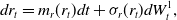 \begin{equation} dr_t=m_r(r_t)dt+\sigma_r(r_t)dW^1_t,\end{equation}
 \begin{equation} d\mu^x_t=m_{\mu}(\mu^x_t)dt+\sigma_{\mu}(\mu^x_t)dW^2_t,\end{equation}
while, without loss of generality and to simplify matters, the reference fund where the insurer invests the policy premiums is supposed to be made up of equities of the same kind, having value $S_t$
at time t and fluctuations described under
$S_t$
at time t and fluctuations described under $\mathbb{Q}$
by the equation
$\mathbb{Q}$
by the equation
 \begin{equation} dS_t=m_S(r_t,S_t)dt+\sigma_S(S_t)dW^3_t.\end{equation}
The Brownian motions $W^i_t$
, with
$W^i_t$
, with $i=1,2,3$
, are pairwise correlated with correlation coefficient
$i=1,2,3$
, are pairwise correlated with correlation coefficient $\rho_{ij}$
, with
$\rho_{ij}$
, with $i,j=1,2,3,i\neq j$
. This structure allows introducing correlations also between financial and actuarial risks. Clearly, the existence of an equivalent martingale measure
$i,j=1,2,3,i\neq j$
. This structure allows introducing correlations also between financial and actuarial risks. Clearly, the existence of an equivalent martingale measure $\mathbb{Q}$
has to be verified for special choices of the market coefficients in the SDEs of
$\mathbb{Q}$
has to be verified for special choices of the market coefficients in the SDEs of $r_t$
,
$r_t$
, $\mu_t^x,$
and
$\mu_t^x,$
and $S_t$
with the help of Girsanov’s theorem.
$S_t$
with the help of Girsanov’s theorem.
In this framework, we may treat different models by simply specifying differently the form of $m_r(r_t)$
and
$m_r(r_t)$
and $\sigma_r(r_t)$
,
$\sigma_r(r_t)$
, $m_\mu(\mu^x_t)$
and
$m_\mu(\mu^x_t)$
and $\sigma_\mu(\mu^x_t)$
, and
$\sigma_\mu(\mu^x_t)$
, and $m_S(r_t,S_t)$
and
$m_S(r_t,S_t)$
and $\sigma_S(S_t)$
. This aspect is of great importance because, for instance, it allows us to take into account more realistic models for capturing the interest rate fluctuations in the financial market where, specially in Europe, sometimes they show a negative pattern, that is, the Vasicek (Reference Vasicek1977) and the Hull and White (Reference Hull and White1993) models are examples of processes that can capture this aspect. Indeed, for instance, defining in (2.1)
$\sigma_S(S_t)$
. This aspect is of great importance because, for instance, it allows us to take into account more realistic models for capturing the interest rate fluctuations in the financial market where, specially in Europe, sometimes they show a negative pattern, that is, the Vasicek (Reference Vasicek1977) and the Hull and White (Reference Hull and White1993) models are examples of processes that can capture this aspect. Indeed, for instance, defining in (2.1) $m_r(r_t)=\kappa_r(\theta_r-r_t)$
and
$m_r(r_t)=\kappa_r(\theta_r-r_t)$
and $\sigma_r(r_t)=\sigma_r$
or
$\sigma_r(r_t)=\sigma_r$
or $\sigma_r(r_t)=\sigma_r\sqrt{r_t}$
, with
$\sigma_r(r_t)=\sigma_r\sqrt{r_t}$
, with $\kappa_r,\theta_r,\sigma_r$
constants and positive, we manage the Vasicek (Reference Vasicek1977) or the Cox et al. (Reference Cox, Ingersoll and Ross1985) model for interest rate, respectively. Similarly, it may be done for the mortality process in (2.2) detailing differently
$\kappa_r,\theta_r,\sigma_r$
constants and positive, we manage the Vasicek (Reference Vasicek1977) or the Cox et al. (Reference Cox, Ingersoll and Ross1985) model for interest rate, respectively. Similarly, it may be done for the mortality process in (2.2) detailing differently $m_{\mu}(\mu^x_t)$
and
$m_{\mu}(\mu^x_t)$
and $\sigma_{\mu}(\mu^x_t)$
(see, for instance, Dahl, Reference Dahl2004, Luciano and Vigna, Reference Luciano and Vigna2005, and Zeddouk and Devolder, Reference Zeddouk and Devolder2020), and for the equity process (2.3) choosing opportunely
$\sigma_{\mu}(\mu^x_t)$
(see, for instance, Dahl, Reference Dahl2004, Luciano and Vigna, Reference Luciano and Vigna2005, and Zeddouk and Devolder, Reference Zeddouk and Devolder2020), and for the equity process (2.3) choosing opportunely $m_S(r_t,S_t)$
and
$m_S(r_t,S_t)$
and $\sigma_S(S_t)$
.
$\sigma_S(S_t)$
.
In the section devoted to the presentation of numerical experiments, we apply this framework to evaluate, for instance, equity-linked term policies and equity-linked endowment policies with or without embedding a surrender option. This is done to provide just some examples of the model applications but, clearly, different contract specifications may be easily managed through the proposed method. Suppose to consider, for example, an equity-linked term policy in absence of the possibility of surrendering the contract early. In case of survival at maturity T, the policy pays an amount of money given by the maximum between the reference fund value at time T, $S_T$
, and the value of the minimum guaranteed amount that, without loss of generality, we suppose to be constant at level G, that is,
$S_T$
, and the value of the minimum guaranteed amount that, without loss of generality, we suppose to be constant at level G, that is, $\max(S_T,G)$
. Following the decomposition suggested by Brennan and Schwartz (Reference Brennan and Schwartz1976), the policy payoff at maturity may be written as
$\max(S_T,G)$
. Following the decomposition suggested by Brennan and Schwartz (Reference Brennan and Schwartz1976), the policy payoff at maturity may be written as $S_T+(G-S_T)^+$
where
$S_T+(G-S_T)^+$
where $(G-S_T)^+=\max(G-S_T,0)$
, that is, as the sum of the value of the reference fund at maturity,
$(G-S_T)^+=\max(G-S_T,0)$
, that is, as the sum of the value of the reference fund at maturity, $S_T$
, and of a put option written on the fund with strike price G, or as
$S_T$
, and of a put option written on the fund with strike price G, or as $G+(S_T-G)^+$
where
$G+(S_T-G)^+$
where $(S_T-G)^+=\max(S_T-G,0)$
, that is, as the sum of the value of the guaranteed amount, G, and of a call option written on the fund with strike price G. For instance, supposing to consider the put-decomposition, in absence of any surrender option, the equity-linked term policy value at time t under the risk-neutral measure
$(S_T-G)^+=\max(S_T-G,0)$
, that is, as the sum of the value of the guaranteed amount, G, and of a call option written on the fund with strike price G. For instance, supposing to consider the put-decomposition, in absence of any surrender option, the equity-linked term policy value at time t under the risk-neutral measure $\mathbb{Q}$
is computed as
$\mathbb{Q}$
is computed as
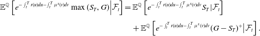 \begin{align*} \mathbb{E}^{\mathbb{Q}}\left[e^{-\int_t^T r(u)du-\int_t^T \mu^x(v)dv}\max(S_T,G)\Big\vert \mathcal{F}_t\right] & = \mathbb{E}^\mathbb{Q} \left[e^{-\int_t^T r(u)du-\int_t^T \mu^x(v)dv}S_T\vert \mathcal{F}_t\right]\\[4pt]& \quad +\mathbb{E}^\mathbb{Q} \left[e^{-\int_t^T r(u)du-\int_t^T \mu^x(v)dv}(G-S_T)^+\big\vert \mathcal{F}_t\right].\nonumber \end{align*}
Whenever the equity-linked term policy embeds a surrender option, the policyholder may exercise the option at any time before maturity thus escaping out of the contract by receiving a pre-specified surrender amount. The exercise of the surrender option is optimal on a financial point of view since the policyholder is a rational individual and, clearly, she/he follows a surrender strategy that is strictly dependent upon the type of the embedded guarantee. Without loss of generality, we model the surrender benefit as $\max(S_t,G)$
and the value of the policy contract at a generic time t may be written as
$\max(S_t,G)$
and the value of the policy contract at a generic time t may be written as
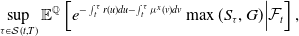 \begin{equation*} \sup_{\tau \in \mathcal{S}(t,T)}\mathbb{E}^{\mathbb{Q}}\left[e^{-\int_t^\tau r(u)du-\int_t^\tau \mu^x(v)dv}\max(S_\tau,G)\Big\vert \mathcal{F}_t\right],\nonumber \end{equation*}
where $\mathcal{S}(t,T)$
indicates the set of all the stopping times of the filtration
$\mathcal{S}(t,T)$
indicates the set of all the stopping times of the filtration $(\mathcal{F}_t)_{0\leq t \leq T}$
between t and T.
$(\mathcal{F}_t)_{0\leq t \leq T}$
between t and T.
Different specifications of the framework may be easily included by considering, for example, a continuous fee paid by the policyholder to have the minimum guarantee that fulfils the role of providing protection against the risk of a negative performance of the reference fund during the policy lifetime. In this case, part of the policy premium is paid by the policyholder for the guarantee and it may be supposed to be collected as a fee continuously withdrawn from the fund at a constant rate $\alpha$
, that is, the reference fund dynamics under the risk-neutral probability measure
$\alpha$
, that is, the reference fund dynamics under the risk-neutral probability measure $\mathbb{Q}$
will be given by
$\mathbb{Q}$
will be given by
 \begin{equation*} dS_t=m_S(r_t,\alpha,S_t)dt+\sigma_S(S_t)dW^3_t,\nonumber\end{equation*}
in which, among others, by considering a Black-Scholes dynamics, we have $m_S(r_t,\alpha,S_t)=(r_t-\alpha)S_t$
and
$m_S(r_t,\alpha,S_t)=(r_t-\alpha)S_t$
and $\sigma_S(S_t)=\sigma_S S_t$
where
$\sigma_S(S_t)=\sigma_S S_t$
where $\sigma_S$
is a positive parameter. In addition, for what concerns the policy contract, we can easily embed an early surrender penalty having, for example, the form
$\sigma_S$
is a positive parameter. In addition, for what concerns the policy contract, we can easily embed an early surrender penalty having, for example, the form $e^{-\kappa(T-t)}$
, where
$e^{-\kappa(T-t)}$
, where $\kappa>0$
represents the constant penalty rate. The effect of the penalty decreases when t increases and vanishes if the policyholder maintains the contract until its maturity so that, supposing to consider still the previous equity-linked term policy, the surrender benefit has the form
$\kappa>0$
represents the constant penalty rate. The effect of the penalty decreases when t increases and vanishes if the policyholder maintains the contract until its maturity so that, supposing to consider still the previous equity-linked term policy, the surrender benefit has the form $e^{-\kappa(T-t)}\max(S_t,G_t)$
. In this particular case, the value of the policy contract may be written as the following optimal stopping problem,
$e^{-\kappa(T-t)}\max(S_t,G_t)$
. In this particular case, the value of the policy contract may be written as the following optimal stopping problem,
 \begin{equation*} \sup_{\tau \in \mathcal{S}(t,T)}\mathbb{E}^{\mathbb{Q}} \left[e^{-\int_t^\tau r(u)du-\int_t^\tau \mu^x(v)dv}\left(e^{-\kappa(T-\tau)}\max(S_{\tau},G)\right)\Big\vert \mathcal{F}_t\right].\nonumber \end{equation*}
The proposed algorithm starts by discretizing the interest rate process (2.1) on the interval [0,T] through a recombining lattice, as detailed in Section 2.2. Then, a similar lattice is used to discretize the mortality rate process (2.2), as reported in Section 2.3. Finally, in Section 2.4, we provide the discretization of the equity process taking into account that its drift depends upon the interest rate process value. We evidence that in all the proposed discretization, we always work under the risk-neutral probability measure.
2.2. The interest rate process discretization
The interest rate process (2.1) is discretized by generating a binomial tree having a number of nodes that grows up linearly with the number of time steps, as detailed in the Costabile and Massabó (Reference Costabile and Massabó2010) approach. A similar discretization for the interest rate may be also found in Costabile et al. (Reference Costabile, Massabó, Russo and Staino2021) and De Angelis et al. (Reference De Angelis, De Marchis, Martire and Russo2022).
As usual, the definition of a lattice method starts by splitting the time horizon [0,T] into n intervals with equal width $\Delta t=T/n$
. For
$\Delta t=T/n$
. For $i=0,\ldots,n$
, node (i,0) is the lowest node at time
$i=0,\ldots,n$
, node (i,0) is the lowest node at time $i\Delta t$
, node (i,1) is the second lowest one and so on, while
$i\Delta t$
, node (i,1) is the second lowest one and so on, while $r(i,j),j=0,\ldots,i$
, is the value of the interest rate at node (i, j) of the discrete process. Clearly, the tree is rooted at
$r(i,j),j=0,\ldots,i$
, is the value of the interest rate at node (i, j) of the discrete process. Clearly, the tree is rooted at $r(0,0)=r_0$
and the other values that approximate the r-process in (2.1) at the i-th time interval are generated as follows:
$r(0,0)=r_0$
and the other values that approximate the r-process in (2.1) at the i-th time interval are generated as follows:
-
on the highest path, $r(i,i)=r(i-1,i-1)+\sigma_r(r(i-1,i-1))\sqrt{\Delta t}$
;
$r(i,i)=r(i-1,i-1)+\sigma_r(r(i-1,i-1))\sqrt{\Delta t}$
; -
on the lowest path, two possible cases arise according to the form considered for
$\sigma_r(r_t)$
in (2.1). Among others, if
$\sigma_r(r_t)=\sigma_r$
like in the Vasicek (Reference Vasicek1977) model, the interest rate process may assume negative values, so that we generate
$r(i,0)=r(i-1,0)-\sigma_r(r(i-1,0))\sqrt{\Delta t}$
; if we define
$\sigma_r(r_t)=\sigma_r\sqrt{r_t}$
, like in the Cox et al. (Reference Cox, Ingersoll and Ross1985) model, the interest rate process may assume only non-negative values and we generate
$r(i,0)=\max(r(i-1,0)-\sigma_r(r(i-1,0))\sqrt{\Delta t},0)$
; -
for all the nodes (i, j) falling between the highest and lowest path, where
$i=2,\ldots,n$
and
$j=1,\ldots,i-1$
, we generate
$r(i,j)=r(i-2,j-1)$
.


It means that the lattice node values are generated starting from the two edges where the construction coincides with the Cox and Rubinstein (Reference Cox and Rubinstein1985) scheme, while the internal lattice node values are defined by generating horizontal layers of nodes starting from the nodes on the two edges. In this way, the resulting lattice is characterized by a recombining shape that allows retaining the computational simplicity of the discretization in that the number of nodes grows linearly in the number of time steps. To complete the definition of the discrete-time approximating process, we need to define the transition probabilities associated with each node (i, j). Transition probabilities of an upward, $p_r(i,j)$
, or a downward,
$p_r(i,j)$
, or a downward, $q_r(i,j)=1-p_r(i,j)$
, movement (when starting from a generic value r(i, j)) are defined in order to replicate the interest rate expected value in the next time interval, that is,
$q_r(i,j)=1-p_r(i,j)$
, movement (when starting from a generic value r(i, j)) are defined in order to replicate the interest rate expected value in the next time interval, that is,
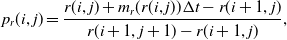 \begin{equation} p_r(i,j) = \frac{r(i, j)+m_r(r(i,j))\Delta t - r(i + 1,j)}{r(i + 1, j + 1) -r(i + 1, j)},\end{equation}
and ensure also to replicate the second order local moment of the continuous-time distribution, at least within the limit.
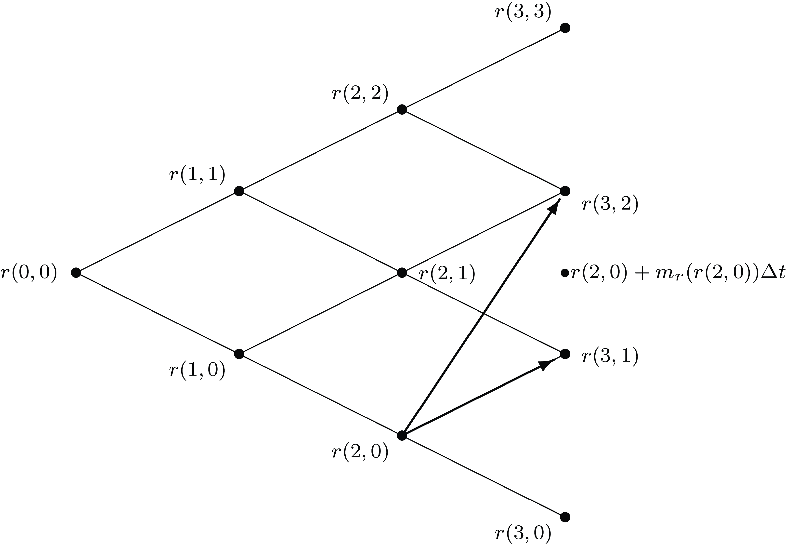
Figure 1. Example of multiple jumps in the r-process.
Whenever relation (2.4) does not return a legitimate probability, that is, a number between 0 and 1, multiple upward or downward jumps are allowed. It happens when $r(i, j) + m_r(r(i,j))\Delta t$
does not lay between
$r(i, j) + m_r(r(i,j))\Delta t$
does not lay between $r(i + 1, j+1)$
and
$r(i + 1, j+1)$
and $r(i + 1, j)$
and an example is given in Figure 1. Here, when the discrete process is at node (2, 0), its expected value is
$r(i + 1, j)$
and an example is given in Figure 1. Here, when the discrete process is at node (2, 0), its expected value is $r(2, 0) + m_r(r(2, 0))\Delta t$
. Hence, the successors cannot be r(3, 1) and r(3, 0) because they do not bracket the expected value, and the resulting transition probability will fall outside the interval [0, 1]. The algorithm chooses the successors of r(2, 0) as the two closest values
$r(2, 0) + m_r(r(2, 0))\Delta t$
. Hence, the successors cannot be r(3, 1) and r(3, 0) because they do not bracket the expected value, and the resulting transition probability will fall outside the interval [0, 1]. The algorithm chooses the successors of r(2, 0) as the two closest values $r(3, j), j = 0,\ldots, 3,$
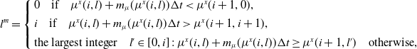
bracketing the expected value of the process (in Figure 1, they are r(3, 2) and r(3, 1)). In formulae, a multiple jump when the process is located at node (i, j) is obtained by defining
$r(3, j), j = 0,\ldots, 3,$
bracketing the expected value of the process (in Figure 1, they are r(3, 2) and r(3, 1)). In formulae, a multiple jump when the process is located at node (i, j) is obtained by defining $j^m$
as
$j^m$
as
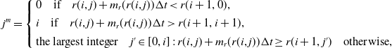 \begin{equation*} j^m=\left\{\begin{array}{l} 0 \quad \text{if} \quad r(i,j) +m_r(r(i,j))\Delta t < r(i + 1, 0),\\[4pt]i \quad \text{if} \quad r(i, j) + m_r(r(i,j))\Delta t > r(i + 1, i+1),\\[4pt]\text{the largest integer} \quad j'\in[0,i]\,:\,r(i, j) +m_r(r(i,j))\Delta t \geq r(i + 1, j') \quad \text{otherwise},\end{array}\right.\nonumber\end{equation*}
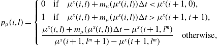
so that the successors are identified as $r(i+1,j^m+1)$
and
$r(i+1,j^m+1)$
and $r(i+1,j^m)$
with transition probabilities
$r(i+1,j^m)$
with transition probabilities
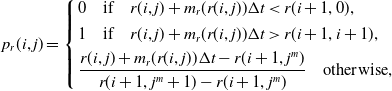 \begin{equation*} p_r(i, j) =\left\{\begin{array}{l} 0 \quad \text{if} \quad r(i, j) + m_r(r(i,j))\Delta t < r(i + 1, 0),\\[4pt]1 \quad \text{if} \quad r(i, j) + m_r(r(i,j))\Delta t > r(i + 1,i+1),\\[4pt]\dfrac{r(i, j) + m_r(r(i,j))\Delta t - r(i + 1, j^m)}{r(i + 1, j^m +1) - r(i + 1, j^m)} \quad \text{otherwise},\end{array}\right.\nonumber\end{equation*}
and $q_r(i,j)=1-p_r(i,j)$
, respectively.
$q_r(i,j)=1-p_r(i,j)$
, respectively.
2.3. The mortality rate process discretization
The procedure detailed in Section 2.2 is also applied to discretize the mortality rate process (2.2) but, in this case, we evidence that it is reasonable to consider only non-negative values for such a process. As a consequence, the lattice is cut at zero on the lowest path.Footnote 1 Briefly, denoting by $\mu^x(i,l),i=0,\ldots,$ $n,l=0,\ldots,i$
, the value of the mortality rate at node (i, l), and rooting the tree at
$n,l=0,\ldots,i$
, the value of the mortality rate at node (i, l), and rooting the tree at $\mu^x(0,0)=\mu^x_0$
, we directly approximate the
$\mu^x(0,0)=\mu^x_0$
, we directly approximate the $\mu^x$
-process in (2.2) as follows:
$\mu^x$
-process in (2.2) as follows:
-
on the highest path,
$\mu^x(i,i)=\mu^x(i-1,i-1)+\sigma_{\mu}(\mu^x(i-1,i-1))\sqrt{\Delta t}$
; -
on the lowest path,
$\mu^x(i,0)=\max(\mu^x(i-1,0)-\sigma_{\mu}(\mu^x(i-1,0))\sqrt{\Delta t},0)$
; and -
on the inner nodes (i, l), where
$i=2,\ldots,n$
and
$l=1,\ldots,i-1$
,
$\mu^x(i,l)=\mu^x(i-2,l-1)$
.


Upward, $p_{\mu}(i,l)$
, and downward,
$p_{\mu}(i,l)$
, and downward, $q_{\mu}(i,j)=1-p_{\mu}(i,l)$
, transition probabilities are defined in order to replicate the mortality intensity expected value in the next time interval, that is,
$q_{\mu}(i,j)=1-p_{\mu}(i,l)$
, transition probabilities are defined in order to replicate the mortality intensity expected value in the next time interval, that is,
 \begin{equation} p_{\mu}(i,l) = \frac{\mu^x(i, l) + m_{\mu}(\mu^x(i,l))\Delta t - \mu^x(i + 1,l)}{\mu^x(i + 1, l + 1) -\mu^x(i + 1, l)},\end{equation}
and they replicate also the second order local moment of the continuous-time distribution, at least within the limit. Whenever relation (2.5) does not ensure that $p_{\mu}(i,l)$
is between 0 and 1, as before we define multiple jumps as
$p_{\mu}(i,l)$
is between 0 and 1, as before we define multiple jumps as
 \begin{equation*} l^m=\left\{\begin{array}{l} 0 \quad \text{if} \quad \mu^x(i,l) +m_{\mu}(\mu^x(i,l))\Delta t < \mu^x(i + 1, 0),\\[4pt]i \quad \text{if} \quad \mu^x(i, l) + m_{\mu}(\mu^x(i,l))\Delta t > \mu^x(i + 1, i+1),\\[4pt]\text{the largest integer} \quad l'\in[0,i]\,:\,\mu^x(i, l) +m_{\mu}(\mu^x(i,l))\Delta t \geq \mu^x(i + 1, l') \quad \text{otherwise},\end{array}\right.\nonumber\end{equation*}
and transition probabilities as
 \begin{equation*} p_{\mu}(i, l) =\left\{\begin{array}{l} 0 \quad \text{if} \quad \mu^x(i, l) + m_{\mu}(\mu^x(i,l))\Delta t < \mu^x(i + 1, 0),\\[4pt]1 \quad \text{if} \quad \mu^x(i, l) + m_{\mu}(\mu^x(i,l))\Delta t > \mu^x(i + 1,i+1),\\[4pt]\dfrac{\mu^x(i, l) + m_{\mu}(\mu^x(i,l))\Delta t - \mu^x(i + 1, l^m)}{\mu^x(i + 1, l^m +1) - \mu^x(i + 1, l^m)} \quad \text{otherwise},\end{array}\right.\nonumber\end{equation*}
and $q_{\mu}(i,l)=1-p_{\mu}(i,l)$
, respectively.
$q_{\mu}(i,l)=1-p_{\mu}(i,l)$
, respectively.
2.4. The equity process discretization
To discretize the equity process (2.3), we have to take into account that its drift depends upon the value registered for the interest rate at a given time step. Hence, at first, as already done above, we proceed to discretize the diffusion part of the process and, then, we will capture the drift effect when computing the transition probabilities associated with each jump.
Denoting by $S(i,h),i=0,\ldots,n,h=0,\ldots,i$
, the equity value of the approximating process at node (i, h), and rooting the tree at
$S(i,h),i=0,\ldots,n,h=0,\ldots,i$
, the equity value of the approximating process at node (i, h), and rooting the tree at $S(0,0)=S_0$
, we approximate the diffusion part S-process in (2.3) as follows:
$S(0,0)=S_0$
, we approximate the diffusion part S-process in (2.3) as follows:
-
on the highest path,
$S(i,i)=S(i-1,i-1)+\sigma_S(S(i-1,i-1))\sqrt{\Delta t}$
; -
as before, on the lowest path, we can give attention to the specification given for
$\sigma_S(S_t)$
. For instance, supposing that
$\sigma_S(S_t)=\sigma_SS_t$
as in the standard Brownian motion, we compute at each step the quantity
$S(i,0)=S(i-1,0)-\sigma_S(S(i-1,0))\sqrt{\Delta t}$
; -
on the inner nodes (i, h), where
$i=2,\ldots,n$
and
$h=1,\ldots,i-1$
,
$S(i,h)=S(i-2,h-1)$
.


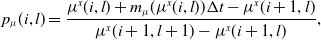
To define the probability that the equity value shows an upward or a downward jump, we have to take into account that the asset price process (2.3) is affected by the stochastic interest rate dynamic. Hence, for each possible interest rate determination, transition probabilities in the discrete model are defined in order to match the first and second order local moments of the continuous-time model, at least within the limit. With this aim, we define a “state of nature” as the triplet (i, j, h) in which the interest rate value is r(i, j) and the equity value is S(i, h), thus computing the upward probability as
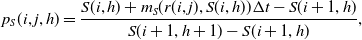 \begin{equation*} p_S(i,j,h)=\frac{S(i,h)+m_S(r(i,j),S(i,h))\Delta t-S(i+1,h)}{S(i+1,h+1)-S(i+1,h)},\nonumber\end{equation*}
and downward probability as $q_S(i,j,h)=1-p_S(i,j,h)$
.
$q_S(i,j,h)=1-p_S(i,j,h)$
.
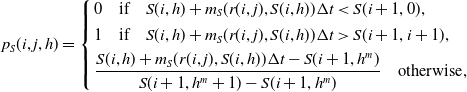
Whenever, multiple jumps are required to keep the value of $p_S(i,j,h)$
within the interval [0, 1], we define
$p_S(i,j,h)$
within the interval [0, 1], we define $h^m$
as
$h^m$
as
 \begin{equation*} h^m=\left\{\begin{array}{l} 0 \quad \text{if} \quad S(i,h) +m_S(r(i,j),S(i,h))\Delta t < S(i + 1, 0),\\[4pt]i \quad \text{if} \quad S(i, h) + m_S(r(i,j),S(i,h))\Delta t > S(i + 1, i+1),\\[4pt]\text{the largest integer} \quad h'\in[0,i]:S(i, h) +m_S(r(i,j),S(i,h))\Delta t \geq S(i + 1, h') \quad \text{otherwise},\end{array}\right.\nonumber\end{equation*}
so that the successors are $S(i+1,l^m+1)$
and
$S(i+1,l^m+1)$
and $S(i+1,l^m)$
with transition probabilities
$S(i+1,l^m)$
with transition probabilities
 \begin{equation*} p_S(i, j,h) =\left\{\begin{array}{l} 0 \quad \text{if} \quad S(i, h) + m_S(r(i,j),S(i,h))\Delta t < S(i + 1, 0),\\[4pt]1 \quad \text{if} \quad S(i, h) + m_S(r(i,j),S(i,h))\Delta t > S(i + 1,i+1),\\[4pt]\dfrac{S(i, h) + m_S(r(i,j),S(i,h))\Delta t - S(i + 1, h^m)}{S(i + 1, h^m +1) - S(i + 1, h^m)} \quad \text{otherwise},\end{array}\right.\nonumber\end{equation*}
and $q_S(i,j,h)=1-p_S(i,j,h)$
, respectively.
$q_S(i,j,h)=1-p_S(i,j,h)$
, respectively.
3. Valuation of bonds through a bivariate discrete model
The discretizations of the three processes provided in Section 2 may be combined in order to create evaluation models for insurance products. A first application we would like to propose is relative to the construction of a bivariate model that combines the two discretizations of the interest and mortality rates. The idea is similar to the one adopted by Costabile et al. (Reference Costabile, Massabó, Russo and Staino2021) and De Angelis et al. (Reference De Angelis, De Marchis, Martire and Russo2022) to develop their bivariate lattice, but the lattice construction is different on some aspects as detailed hereafter and, more important, it has a different aim, that is, the introduction of the mortality risk in the evaluation process. Under this perspective, we choose to evaluate survival zero coupon bonds paying one unit of money at maturity in case of survival and mortality bonds characterized by traditional fixed coupons at regular intervals and a principal at maturity becoming random and linked with realized longevity or mortality experiences. The aim is to show the impact of the correlation structure characterizing the two processes upon the bond values but, clearly, other products like interest sensitive claims may be easily evaluated by the generated model embedding the mortality risk.
3.1. The bivariate lattice and the joint branching probabilities
The lattices discretizing the r-process and the $\mu$
-process are combined into a sort of pyramid where each node is linked to four branches. The probability associated with each branch is computed by the product of the corresponding marginal probabilities in the lattice for
$\mu$
-process are combined into a sort of pyramid where each node is linked to four branches. The probability associated with each branch is computed by the product of the corresponding marginal probabilities in the lattice for $r_t$
and
$r_t$
and $\mu^x_t$
plus an adjusting addendum in order to take into account the process correlation. The pyramid is obtained by defining a state of nature as a triplet (i, j, l) with
$\mu^x_t$
plus an adjusting addendum in order to take into account the process correlation. The pyramid is obtained by defining a state of nature as a triplet (i, j, l) with $i=0,\ldots,n$
, and
$i=0,\ldots,n$
, and $j,l=0,\ldots,i$
, in correspondence of which the interest rate assumes value r(i, j) and the mortality rate has value
$j,l=0,\ldots,i$
, in correspondence of which the interest rate assumes value r(i, j) and the mortality rate has value $\mu^x(i,l)$
. Starting from a generic state (i, j, l), all the possible movements of the resulting joint process are captured by four scenarios labelled by a pair in which the first element refers to the r-process movement, upward denoted by “u”, or downward denoted by “d”, while the second element refers to the
$\mu^x(i,l)$
. Starting from a generic state (i, j, l), all the possible movements of the resulting joint process are captured by four scenarios labelled by a pair in which the first element refers to the r-process movement, upward denoted by “u”, or downward denoted by “d”, while the second element refers to the $\mu$
-movement. For instance, the pair ud identifies the branch with an upward movement in the r-dynamic and a downward movement in the
$\mu$
-movement. For instance, the pair ud identifies the branch with an upward movement in the r-dynamic and a downward movement in the $\mu$
-dynamic.
$\mu$
-dynamic.
The transition probabilities in correspondence of each scenario, $p_{uu},p_{ud},p_{du}$
, and
$p_{uu},p_{ud},p_{du}$
, and $p_{dd}$
, are obtained by solving the linear system arising by considering the following four conditions:
$p_{dd}$
, are obtained by solving the linear system arising by considering the following four conditions:
-
1. the probabilities sum is equal to 1,
(3.1)
\begin{equation} p_{uu}+p_{ud}+p_{du}+p_{dd}=1;\end{equation}
-
2. the marginal probability of the r-process is replicated, that is,
(3.2)
\begin{equation} p_{uu}+p_{ud}=p_r(i,j);\end{equation}
-
3. the marginal probability of the
$\mu$
-process is replicated, that is,(3.3)
\begin{equation} p_{uu}+p_{du}=p_{\mu}(i,l);\, \text{and}\end{equation}
-
4. the covariance between the discrete r-process and
$\mu$
-process must equal the covariance between the continuous-time processes, that is,(3.4)
\begin{equation} p_{uu}-p_{ud}-p_{du}+p_{dd}=\rho_{12}.\end{equation}


Solving simultaneously Equations (3.1)–(3.4), we obtain the following solutions:
 \[p_{uu}=p_r(i,j)p_{\mu}(i,l)+\frac{\rho_{12}}{4};\quad p_{ud}=p_r(i,j)q_\mu(i,l)-\frac{\rho_{12}}{4};\]
 \[ p_{du}=q_r(i,j)p_\mu(i,l)-\frac{\rho_{12}}{4};\quad \text{and}\quad p_{dd}=q_r(i,j)q_\mu(i,l)+\frac{\rho_{12}}{4}.\]
It is worth noting that all the probabilities above belong to the interval [0, 1] in the limit, that is, when the number of time steps n used to discretize the r-process and the $\mu^x$
-process tends to infinity. To show this aspect, consider for instance the probability
$\mu^x$
-process tends to infinity. To show this aspect, consider for instance the probability $p_{uu}$
for which we have
$p_{uu}$
for which we have $0 \leq p_{uu} \leq 1$
if
$0 \leq p_{uu} \leq 1$
if $-\frac{\rho_{12}}{4} \leq p_r(i,j)p_{\mu}(i,l)\leq 1-\frac{\rho_{12}}{4}$
, with
$-\frac{\rho_{12}}{4} \leq p_r(i,j)p_{\mu}(i,l)\leq 1-\frac{\rho_{12}}{4}$
, with $-1 \leq \rho_{12} \leq 1$
. The previous double inequality is always satisfied for any value of
$-1 \leq \rho_{12} \leq 1$
. The previous double inequality is always satisfied for any value of $\rho_{12}$
if
$\rho_{12}$
if $\frac{1}{4} \leq p_r(i,j)p_{\mu}(i,l)\leq \frac{3}{4}$
. The latter is always true when
$\frac{1}{4} \leq p_r(i,j)p_{\mu}(i,l)\leq \frac{3}{4}$
. The latter is always true when $n\rightarrow +\infty$
because
$n\rightarrow +\infty$
because $p_r(i,j)\rightarrow \frac{1}{2}$
and
$p_r(i,j)\rightarrow \frac{1}{2}$
and $p_{\mu}(i,l)\rightarrow \frac{1}{2}$
as
$p_{\mu}(i,l)\rightarrow \frac{1}{2}$
as $n\rightarrow +\infty$
.Footnote 2
$n\rightarrow +\infty$
.Footnote 2
3.2. Survival zero coupon bonds
We apply the proposed bivariate model for evaluating a survival zero coupon bond paying one unit of money at maturity T in case of survival, which in a continuous time framework it is equivalent to compute the expected value $\mathbb{E}^{\mathbb{Q}}\left[e^{-\int_t^T r(u)du-\int_t^T \mu^x(v)dv}\right]$
under the risk-neutral probability measure
$\mathbb{E}^{\mathbb{Q}}\left[e^{-\int_t^T r(u)du-\int_t^T \mu^x(v)dv}\right]$
under the risk-neutral probability measure $\mathbb{Q}$
imposing
$\mathbb{Q}$
imposing $t=0$
. To compute the fair bond value at inception, we have to use the proposed discretization proceeding backward on the bivariate tree. We label by B(i, j, l),
$t=0$
. To compute the fair bond value at inception, we have to use the proposed discretization proceeding backward on the bivariate tree. We label by B(i, j, l), $i=0,\ldots,n;\, j,l=0,\ldots,i$
, the fair bond value when the interest rate is located at node (i, j) and the mortality rate at node (i, l). At maturity, on the terminal state of nature (n, j, l), the bond value is given by
$i=0,\ldots,n;\, j,l=0,\ldots,i$
, the fair bond value when the interest rate is located at node (i, j) and the mortality rate at node (i, l). At maturity, on the terminal state of nature (n, j, l), the bond value is given by
 \begin{equation} B(n,j,l)=1,\end{equation}
and, proceeding backward, the fair bond value in state of nature (i, j, l) is computed as
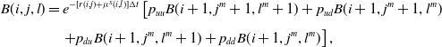 \begin{align} B(i,j,l) & = e^{-[r(i,j)+\mu^x(i,l)]\Delta t}\left[p_{uu}B(i+1,j^m+1,l^m+1)+p_{ud}B(i+1,j^m+1,l^m)\right.\nonumber\\[4pt]& \quad \left. + p_{du}B(i+1,j^m,l^m+1)+ p_{dd}B(i+1,j^m,l^m)\right],\end{align}
where we consider properly the interest rate and mortality risks and, for instance, $B(i+1,j^m+1,l^m+1)$
is the fair bond value when, starting from state of nature (i, j, l), all the processes show an upward movement. The backward induction proceeds up to node (0, 0, 0) that contains the fair bond value at the contract inception.
$B(i+1,j^m+1,l^m+1)$
is the fair bond value when, starting from state of nature (i, j, l), all the processes show an upward movement. The backward induction proceeds up to node (0, 0, 0) that contains the fair bond value at the contract inception.
3.3. Mortality bonds
The discretization technique can also be used for the pricing of securitization products based on mortality or longevity risks. Indeed, these products naturally combine financial and actuarial elements and the correlations between them will have a direct influence on their valuation. Securitization for the insurer is based on a mechanism of transfer of risk through financial markets instead of classical reinsurance. For instance, let us consider a bond characterized by traditional fixed coupons at regular intervals and a random principal at maturity, linked with realized longevity or mortality experiences as reported, among others, in Cox and Pedersen (Reference Cox and Pedersen2000) or Lin and Cox (Reference Lin and Cox2008). Still denoting by T the maturity of the bond, by c the fixed coupons annually paid, and by L(T) the stochastic principal to be defined, the initial price at time t (imposing $t<1$
to capture the effect of all the coupons) of the instrument under the risk-neutral probability measure
$t<1$
to capture the effect of all the coupons) of the instrument under the risk-neutral probability measure $\mathbb{Q}$
is given by
$\mathbb{Q}$
is given by
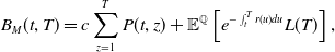 \begin{equation} B_{M}(t,T)=c\sum\limits_{z=1}^{T}P(t,z)+\mathbb{E}^{\mathbb{Q}}\left[e^{-\int_t^T r(u)du}L(T)\right],\end{equation}
where P(t, z) is the value at time t of the classical zero coupon bond price with maturity z, that is, $P(t,z)=\mathbb{E}^{\mathbb{Q}}\left[e^{-\int_t^z r(u)du}\right]$
.
$P(t,z)=\mathbb{E}^{\mathbb{Q}}\left[e^{-\int_t^z r(u)du}\right]$
.
The first term in the right-hand side of Equation (3.7) is very simple and explicit but the second one, through the term L(T), involves simultaneously interest rates and mortality risk with potential correlation. Indeed, depending on the kind of protection asked by the issuer of the bond, the payoff L(T) can be based on survival conditions (longevity risk) or on mortality results. Under this perspective, let us consider here a mortality bond. The purpose of the product is to protect the issuer against possible deviation of the observed mortality compared to a reference value defined ex ante. Assuming that we follow an initial cohort aged x at time t, the payoff is assumed to be given by $L(T)=Kl(T)$
, where K is the nominal of the bond and l(T) is a random variable identifying a loss function comparing the realized level of global mortality between age x and age
$L(T)=Kl(T)$
, where K is the nominal of the bond and l(T) is a random variable identifying a loss function comparing the realized level of global mortality between age x and age $x+(T-t)$
denoted by
$x+(T-t)$
denoted by $q_T$
to a reference level fixed at issuance and denoted by
$q_T$
to a reference level fixed at issuance and denoted by $q_t$
.
$q_t$
.
Let us consider, for instance, a linear product which can be seen as a Forward Rate Agreement at maturity between the observed and the expected mortalities. The loss function is equal to 1 if the realized mortality is equal to the expected one (in that case the bond will pay the normal nominal); if the realized mortality is higher (lower) than the expected one, the bond will pay less (more) than the nominal. In this case, the loss function is then given by $l(T)=1+\lambda(q_t-q_T)$
, where
$l(T)=1+\lambda(q_t-q_T)$
, where $\lambda$
is a positive factor between 0 and 1 (if
$\lambda$
is a positive factor between 0 and 1 (if $\lambda=0$
, there is no correction for mortality; if
$\lambda=0$
, there is no correction for mortality; if $\lambda=1$
, there is a complete recovery of the mortality spread; for
$\lambda=1$
, there is a complete recovery of the mortality spread; for $0<\lambda<1$
, we get a partial recovery). By introducing the corresponding survival rates defined by
$0<\lambda<1$
, we get a partial recovery). By introducing the corresponding survival rates defined by $p_t=1-q_t$
, the loss function becomes
$p_t=1-q_t$
, the loss function becomes $l(T)=1+\lambda(p_T-p_t)$
, so that the payoff of the principal at maturity is given by
$l(T)=1+\lambda(p_T-p_t)$
, so that the payoff of the principal at maturity is given by
 \begin{equation*} L(T)=Kl(T)=K\left[1+\lambda(p_T-p_t)\right]=K-\lambda Kp_t+\lambda Kp_T,\nonumber\end{equation*}
where $p_t$
is fixed while
$p_t$
is fixed while $p_T=e^{-\int_t^T \mu^x(v)dv}$
.
$p_T=e^{-\int_t^T \mu^x(v)dv}$
.
To sum up, the second term in the right-hand side of Equation (3.7) may be written as
 \begin{equation*} \mathbb{E}^{\mathbb{Q}}\left[e^{-\int_t^T r(u)du}L(T)\right]=(K-\lambda Kp_t)\mathbb{E}^{\mathbb{Q}}\left[e^{-\int_t^T r(u)du}\right]+\lambda K \mathbb{E}^{\mathbb{Q}}\left[e^{-\int_t^T r(u)du-\int_t^T \mu^x(v)dv}\right],\nonumber\end{equation*}
so that the mortality bond value at time t is definitively given by
 \begin{equation} B_{M}(t,T)=c\sum\limits_{z=1}^{T}P(t,z)+(K-\lambda Kp_t)\mathbb{E}^{\mathbb{Q}}\left[e^{-\int_t^T r(u)du}\right]+\lambda K \mathbb{E}^{\mathbb{Q}}\left[e^{-\int_t^T r(u)du-\int_t^T \mu^x(v)dv}\right].\end{equation}
To determine the mortality bond value at inception, that is, $t=0$
, through the proposed bivariate model, we have to treat separately the addenda appearing in (3.8). With this aim, we need an additional requirement concerning the number of time steps n used to discretize the time to maturity of the bond, T. Indeed, the presence of the coupon c annually paid implies that we must have a layer of nodes coinciding with each contract year in order to evaluate the present value of all the coupons consistently and without generating biases in the pricing procedure. In this perspective, we choose n as a multiple of T so that we are ensured that each calendar year is discretized through
$t=0$
, through the proposed bivariate model, we have to treat separately the addenda appearing in (3.8). With this aim, we need an additional requirement concerning the number of time steps n used to discretize the time to maturity of the bond, T. Indeed, the presence of the coupon c annually paid implies that we must have a layer of nodes coinciding with each contract year in order to evaluate the present value of all the coupons consistently and without generating biases in the pricing procedure. In this perspective, we choose n as a multiple of T so that we are ensured that each calendar year is discretized through $\frac{n}{T}$
time steps and we have a layer of nodes coinciding with each coupon payment epoch
$\frac{n}{T}$
time steps and we have a layer of nodes coinciding with each coupon payment epoch $z\in\mathbb{N}$
with
$z\in\mathbb{N}$
with $z\in[1,T]$
.
$z\in[1,T]$
.
The last addendum in (3.8) may be easily evaluated by formula (3.6), imposing at maturity $B(n,j,l)=\lambda K$
in formula (3.5). Indeed, it may be seen as a survival zero coupon bond paying the amount
$B(n,j,l)=\lambda K$
in formula (3.5). Indeed, it may be seen as a survival zero coupon bond paying the amount $\lambda K$
at maturity. The valuation of the first two addenda may be done simultaneously in a univariate environment since there is not mortality effect to capture but only a stochastic interest rate dynamics to manage. Hence, they may be seen together as parts of a coupon bond with annual coupon equal to c and nominal value paid at maturity T equal to
$\lambda K$
at maturity. The valuation of the first two addenda may be done simultaneously in a univariate environment since there is not mortality effect to capture but only a stochastic interest rate dynamics to manage. Hence, they may be seen together as parts of a coupon bond with annual coupon equal to c and nominal value paid at maturity T equal to $K-\lambda Kp_0$
, which may be evaluated along the tree developed to discretize the interest rate evolution. To determine the value at inception of such a coupon bond, at maturity T we define the quantity
$K-\lambda Kp_0$
, which may be evaluated along the tree developed to discretize the interest rate evolution. To determine the value at inception of such a coupon bond, at maturity T we define the quantity $B^c(n,j)=K-\lambda Kp_0+c$
, with
$B^c(n,j)=K-\lambda Kp_0+c$
, with $j=0,\ldots, n$
, as the sum of the nominal value plus the last paid coupon, and proceed backward by computing for
$j=0,\ldots, n$
, as the sum of the nominal value plus the last paid coupon, and proceed backward by computing for $i=n-1,\ldots,0$
, and
$i=n-1,\ldots,0$
, and $j=0,\ldots,i$
, the quantity
$j=0,\ldots,i$
, the quantity
 \begin{equation}B^c(i,j)=e^{-r(i,j)\Delta t}\left[p_r(i,j)B^c(i+1,j^m+1)+q_r(i,j)B^c(i+1,j^m)\right]+c \mathbb{I}_{\left\{z\in\mathbb{N}|i\Delta t=z, z\in[1,T-1]\right\}},\nonumber\end{equation}
where $\mathbb{I}_{\{\cdot\}}$
is the indicator function assuming value 1 when
$\mathbb{I}_{\{\cdot\}}$
is the indicator function assuming value 1 when $i\Delta t$
coincides with a contract year and 0 otherwise. Finally, the value of the mortality bond at inception is given by the sum
$i\Delta t$
coincides with a contract year and 0 otherwise. Finally, the value of the mortality bond at inception is given by the sum $B^c(0,0)+B(0,0,0)$
.
$B^c(0,0)+B(0,0,0)$
.
4. Valuation of equity-linked life insurances policies through a trivariate discrete model
A second application we would like to propose in this paper considers contemporaneously all the discretizations of the interest rate, mortality rate, and equity processes and develop an algorithm based on the construction of a trivariate model inspired by a methodology presented in Hilliard and Schwartz (Reference Hilliard and Schwartz1997) and Russo and Staino (Reference Russo and Staino2018a). The aim is to generate an algorithm that is able to evaluate the linked products in the insurance markets and to easily manage the presence of a surrender option that allows the policyholder to escape out of the contract early.
4.1. The trivariate lattice and the joint branching probabilities
The lattices discretizing the r-process, the $\mu$
-process, and the S-process are combined into a trivariate environment where each node has eight branches each one presenting a probability computed by the product of the marginal probabilities of the jumps in the lattice for
$\mu$
-process, and the S-process are combined into a trivariate environment where each node has eight branches each one presenting a probability computed by the product of the marginal probabilities of the jumps in the lattice for $r_t$
,
$r_t$
, $\mu^x_t$
, and
$\mu^x_t$
, and $S_t$
, plus an adjusting addendum to take into account the pairwise process correlations. In detail, here we define a state of nature as a quadruplet (i, j, l, h) with
$S_t$
, plus an adjusting addendum to take into account the pairwise process correlations. In detail, here we define a state of nature as a quadruplet (i, j, l, h) with $i=0,\ldots,n$
, and
$i=0,\ldots,n$
, and $j,l,h=0,\ldots,i$
, in correspondence of which the interest rate assumes value r(i, j), the mortality rate has value
$j,l,h=0,\ldots,i$
, in correspondence of which the interest rate assumes value r(i, j), the mortality rate has value $\mu^x(i,l)$
, and the fund has value S(i, j, h). Starting from a generic state (i, j, l, h), the trivariate lattice presents eight possible scenarios, each one labelled with an ordered triplet. The first element of the triplet refers to the discrete interest rate process, upward denoted by “u” or downward denoted by “d”, the second element refers to the
$\mu^x(i,l)$
, and the fund has value S(i, j, h). Starting from a generic state (i, j, l, h), the trivariate lattice presents eight possible scenarios, each one labelled with an ordered triplet. The first element of the triplet refers to the discrete interest rate process, upward denoted by “u” or downward denoted by “d”, the second element refers to the $\mu^x$
-movement, and the third element to the S-movement. For instance, the triplet uuu identifies the branch in which all the processes show an upward movement, the triplet uud denotes the branch in which the discrete r-dynamics and
$\mu^x$
-movement, and the third element to the S-movement. For instance, the triplet uuu identifies the branch in which all the processes show an upward movement, the triplet uud denotes the branch in which the discrete r-dynamics and $\mu^x$
-dynamics show an upward movement and the discrete S-dynamics shows a downward movement, and so on.
$\mu^x$
-dynamics show an upward movement and the discrete S-dynamics shows a downward movement, and so on.
At this point, we have to define the joint transition probabilities of the resulting model, $p_{uuu},p_{uud},p_{udu},p_{udd},p_{duu},p_{dud},p_{ddu}$
, and
$p_{uuu},p_{uud},p_{udu},p_{udd},p_{duu},p_{dud},p_{ddu}$
, and $p_{ddd}$
, which are computed by solving the linear system arising by considering the conditions detailed hereafter:
$p_{ddd}$
, which are computed by solving the linear system arising by considering the conditions detailed hereafter:
-
1. the probabilities sum is equal to 1,
(4.1)
\begin{equation} p_{uuu}+p_{uud}+p_{udu}+p_{udd}+p_{duu}+p_{dud}+p_{ddu}+p_{ddd}=1;\end{equation}
-
2. the marginal probability of the r-process is replicated, that is,
(4.2)
\begin{equation} p_{uuu}+p_{uud}+ p_{udu}+p_{udd}=p_r(i,j);\end{equation}
-
3. the marginal probability of the
$\mu^x$
-process is replicated, that is,(4.3)
\begin{equation} p_{uuu}+p_{uud}+ p_{duu}+p_{dud}=p_{\mu}(i,l);\end{equation}
-
4. the marginal probability of the S-process is replicated, that is,
(4.4)
\begin{equation} p_{uuu}+p_{udu}+ p_{duu}+p_{ddu}=p_S(i,j,h);\end{equation}
-
5. the covariance between the discrete r-process and
$\mu^x$
-process matches the covariance between the corresponding continuous-time processes, that is,(4.5)
\begin{equation} p_{uuu}+p_{uud}-p_{udu}-p_{udd}-p_{duu}-p_{dud}+p_{ddu}+p_{ddd}=\rho_{12};\end{equation}
-
6. the covariance between the discrete r-process and S-process matches the covariance between the corresponding continuous-time processes, that is,
(4.6)
\begin{equation} p_{uuu}-p_{uud}+p_{udu}-p_{udd}-p_{duu}+p_{dud}-p_{ddu}+p_{ddd}=\rho_{13};\end{equation}
-
7. the covariance between the discrete
$\mu^x$
-process and S-process matches the covariance between the corresponding continuous-time processes, that is,(4.7)
\begin{equation} p_{uuu}-p_{uud}-p_{udu}+p_{udd}+p_{duu}-p_{dud}-p_{ddu}+p_{ddd}=\rho_{23};\end{equation}
-
8. the discrete triple cross product matches the corresponding continuous-time one, that is,
(4.8)
\begin{equation} p_{uuu}-p_{uud}-p_{udu}+p_{udd}-p_{duu}+p_{dud}+p_{ddu}-p_{ddd}=0.\end{equation}


Solving simultaneously Equations (4.1)–(4.8), we obtain the following solutions:
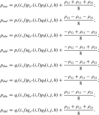 \begin{eqnarray*} p_{uuu} &=& p_r(i,j)p_{\mu^x}(i,l)p_S(i,j,h)+\frac{\rho_{12}+\rho_{13}+\rho_{23}}{8}; \nonumber\\[7pt] p_{uud} &=& p_r(i,j)p_{\mu^x}(i,l)q_S(i,j,h)+\frac{\rho_{12}-\rho_{13}-\rho_{23}}{8}; \nonumber\\[7pt] p_{udu} &=& p_r(i,j)q_{\mu^x}(i,l)p_S(i,j,h)+\frac{-\rho_{12}+\rho_{13}-\rho_{23}}{8}; \nonumber\\[7pt] p_{udd} &=& p_r(i,j)q_{\mu^x}(i,l)q_S(i,j,h)+\frac{-\rho_{12}-\rho_{13}+\rho_{23}}{8};\nonumber \\[7pt] p_{duu} &=& q_r(i,j)p_{\mu^x}(i,l)p_S(i,j,h)+\frac{-\rho_{12}-\rho_{13}+\rho_{23}}{8};\nonumber \\[7pt] p_{dud} &=& q_r(i,j)p_{\mu^x}(i,l)q_S(i,j,h)+\frac{-\rho_{12}+\rho_{13}-\rho_{23}}{8};\nonumber \\[7pt] p_{ddu} &=& q_r(i,j)q_{\mu^x}(i,l)p_S(i,j,h)+\frac{\rho_{12}-\rho_{13}-\rho_{23}}{8};\nonumber \\[7pt] p_{ddd} &=& q_r(i,j)q_{\mu^x}(i,l)q_S(i,j,h)+\frac{\rho_{12}+\rho_{13}+\rho_{23}}{8}.\nonumber\end{eqnarray*}
We have to observe that, substantially, we have four different values for the correction term added to the product of the marginal process probabilities, and, in the solutions above, each one of these four terms is replicated two times. It is easy to prove that all the probabilities of the trivariate model belong to the interval [0, 1], in the limit (i.e., when the number of time steps n used to discretize the r-process, the $\mu^x$
-process and the S-process tends to infinity) when each one of the four different correction terms is greater than
$\mu^x$
-process and the S-process tends to infinity) when each one of the four different correction terms is greater than $-\frac{1}{8}$
. For instance, if we consider
$-\frac{1}{8}$
. For instance, if we consider $p_{uuu}$
, in the limit we have that
$p_{uuu}$
, in the limit we have that $\lim\limits_{n\rightarrow +\infty} p_{uuu}=\frac{1}{8}+\frac{\rho_{12}+\rho_{13}+\rho_{23}}{8}$
because
$\lim\limits_{n\rightarrow +\infty} p_{uuu}=\frac{1}{8}+\frac{\rho_{12}+\rho_{13}+\rho_{23}}{8}$
because $p_r(i,j)\rightarrow \frac{1}{2}$
,
$p_r(i,j)\rightarrow \frac{1}{2}$
, $p_{\mu}(i,l)\rightarrow \frac{1}{2}$
, and
$p_{\mu}(i,l)\rightarrow \frac{1}{2}$
, and $p_S(i,j,h)\rightarrow \frac{1}{2}$
as
$p_S(i,j,h)\rightarrow \frac{1}{2}$
as $n\rightarrow +\infty$
. Hence,
$n\rightarrow +\infty$
. Hence, $0\leq p_{uuu} \leq 1$
in the limit if
$0\leq p_{uuu} \leq 1$
in the limit if $-\frac{1}{8}\leq \frac{\rho_{12}+\rho_{13}+\rho_{23}}{8}\leq \frac{7}{8}$
. The right-hand side inequality is always satisfied so that we have a legitimate probability when
$-\frac{1}{8}\leq \frac{\rho_{12}+\rho_{13}+\rho_{23}}{8}\leq \frac{7}{8}$
. The right-hand side inequality is always satisfied so that we have a legitimate probability when $\frac{\rho_{12}+\rho_{13}+\rho_{23}}{8}\geq -\frac{1}{8}$
. Clearly, there are correlation structures that are admissible in our model but do not satisfy the previous condition. These cases have to be preliminarily investigated if they are of practical utility when valuing a given insurance contract but surely, on a theoretical point of view, they may lead to possible negative probabilities in the trivariate model that can generate instabilities, a well known fact in the literature of finite difference methods for solving PDEs.
$\frac{\rho_{12}+\rho_{13}+\rho_{23}}{8}\geq -\frac{1}{8}$
. Clearly, there are correlation structures that are admissible in our model but do not satisfy the previous condition. These cases have to be preliminarily investigated if they are of practical utility when valuing a given insurance contract but surely, on a theoretical point of view, they may lead to possible negative probabilities in the trivariate model that can generate instabilities, a well known fact in the literature of finite difference methods for solving PDEs.
4.2. Fair value computation of insurance contracts
To determine the fair value of an insurance contract in the proposed framework, we proceed backward along the trivariate lattice computing the policy value in correspondence of each state of nature (i, j, l, h), with $i=0,\ldots,n;\, j,l,h=0,\ldots,i$
. In this sense, we provide a couple of examples of application of the proposed algorithm. We start considering the simplest case of an equity-linked term policy with a minimum guarantee in which, later, we embed a surrender option that allows the policyholder to escape out of the contract before maturity. Then, we consider equity-linked endowment policies with minimum guarantee and surrender option. What we propose are just some possible examples of application of the proposed model but, clearly, it can be also applied to evaluate different contracts like variable annuities, participating policies, etc.
$i=0,\ldots,n;\, j,l,h=0,\ldots,i$
. In this sense, we provide a couple of examples of application of the proposed algorithm. We start considering the simplest case of an equity-linked term policy with a minimum guarantee in which, later, we embed a surrender option that allows the policyholder to escape out of the contract before maturity. Then, we consider equity-linked endowment policies with minimum guarantee and surrender option. What we propose are just some possible examples of application of the proposed model but, clearly, it can be also applied to evaluate different contracts like variable annuities, participating policies, etc.
4.2.1. Equity-linked term policies
We consider an equity-linked term policy characterized by a minimum guarantee having the function of protecting the policyholder’s investment against a bad performance of the fund. It means that the insurer pays at least a minimum amount G that, to simplify matters without loss of generality, we suppose equal to the initial investment $S_0$
, that is,
$S_0$
, that is, $G=S_0$
. More in detail, at maturity, T, the insurer has to pay an amount given by
$G=S_0$
. More in detail, at maturity, T, the insurer has to pay an amount given by $\max[S(T),G]$
. It is worth noting that, to evaluate the policy fair value, we can also refer to the Brennan and Schwartz (Reference Brennan and Schwartz1976) decomposition for the policy payoff at maturity,
$\max[S(T),G]$
. It is worth noting that, to evaluate the policy fair value, we can also refer to the Brennan and Schwartz (Reference Brennan and Schwartz1976) decomposition for the policy payoff at maturity, $\max[S(T),G]$
, evidencing that it is dependent upon a financial option payoff. In particular, they suggested both a put-decomposition as
$\max[S(T),G]$
, evidencing that it is dependent upon a financial option payoff. In particular, they suggested both a put-decomposition as
 \begin{equation} S(T)+\max[G-S(T),0],\end{equation}
and a call-decomposition as
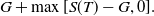 \begin{equation} G+\max[S(T)-G,0].\end{equation}
The decomposition in (4.9) characterizes the policy payoff at maturity as the sum of the fund value plus the payoff of a put option written on the fund with strike price G. Clearly, the option identifies the cost of the guarantee embedded into the contract. On the other hand, the decomposition in (4.10) characterizes the policy payoff at maturity as the sum of the amount G plus the value of a call option on the fund with strike price G.
To compute the fair policy value at inception, we have to use the proposed discretization proceeding backward on the trivariate tree. Supposing to work without considering the Brennan and Schwartz (Reference Brennan and Schwartz1976) decomposition,Footnote 3 we label by FV(i, j, l, h), $i=0,\ldots,n;\, j,l,h=0,\ldots,i$
, the policy fair value when the interest rate is located at node (i, j), the mortality is located at node (i, l), and equity is located at node (i, h). At maturity, on the terminal state of nature (n, j, l, h), the policy value is given by
$i=0,\ldots,n;\, j,l,h=0,\ldots,i$
, the policy fair value when the interest rate is located at node (i, j), the mortality is located at node (i, l), and equity is located at node (i, h). At maturity, on the terminal state of nature (n, j, l, h), the policy value is given by
 \begin{equation*} FV(n,j,l,h)=\max\left[S(n,h),G\right],\nonumber\end{equation*}
and, proceeding backward, the policy fair value in state of nature (i, j, l, h) is computed as
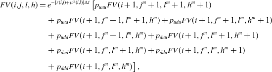 \begin{align*} FV(i,j,l,h) & =e^{-[r(i,j)+\mu^x(i,l)]\Delta t}\left[p_{uuu}FV(i+1,j^m+1,l^m+1,h^m+1)\right.\nonumber\\[4pt]& \quad +\left. p_{uud}FV(i+1,j^m+1,l^m+1,h^m)+p_{udu}FV(i+1,j^m+1,l^m,h^m+1)\right.\nonumber\\[4pt]& \quad +\left. p_{udd}FV(i+1,j^m+1,l^m,h^m)+p_{duu}FV(i+1,j^m,l^m+1,h^m+1)\right.\nonumber\\[4pt]& \quad +\left. p_{dud}FV(i+1,j^m,l^m+1,h^m)+p_{ddu}FV(i+1,j^m,l^m,h^m+1)\right.\nonumber\\[4pt]& \quad +\left. p_{ddd}FV(i+1,j^m,l^m,h^m)\right],\nonumber\end{align*}
where we consider properly the interest rate and mortality risks and, for instance, $FV(i+1,j^m+1,l^m+1,h^m+1)$
is the policy fair value when, starting from state of nature (i, j, l, h), all the processes show an upward movement. The backward induction proceeds up to node (0, 0, 0, 0) that contains the policy fair value at the contract inception.
$FV(i+1,j^m+1,l^m+1,h^m+1)$
is the policy fair value when, starting from state of nature (i, j, l, h), all the processes show an upward movement. The backward induction proceeds up to node (0, 0, 0, 0) that contains the policy fair value at the contract inception.
Now we add to the previous policy contract a surrender option providing the policyholder with the right to terminate the contract early. If the policyholder exercises the surrender option, she/he will receive the surrender value of the contract, SV, depending upon both the current value of the fund and the minimum guaranteed amount, G. We hypothesize that the surrender value is defined as $SV(i,j,l,h)=\max[S(i,h),G]$
.
$SV(i,j,l,h)=\max[S(i,h),G]$
.
To compute the fair policy value at inception, we start again from maturity, where the policy value is still given by
 \begin{equation*} FV(n,j,l,h)=\max\left[S(n,h),G\right],\nonumber\end{equation*}
and, proceeding backward, the policy fair value in state of nature (i, j, l, h) is computed as
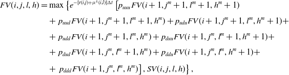 \begin{align*} FV(i,j,l,h) & =\max\left\{e^{-[r(i,j)+\mu^x(i,l)]\Delta t}\left[p_{uuu}FV(i+1,j^m+1,l^m+1,h^m+1)\right.\right.\nonumber\\[4pt]& \quad +\left. p_{uud}FV(i+1,j^m+1,l^m+1,h^m)+p_{udu}FV(i+1,j^m+1,l^m,h^m+1)+\right.\nonumber\\[4pt]& \quad +\left. p_{udd}FV(i+1,j^m+1,l^m,h^m)+p_{duu}FV(i+1,j^m,l^m+1,h^m+1)+\right.\nonumber\\[4pt]& \quad +\left. p_{dud}FV(i+1,j^m,l^m+1,h^m)+p_{ddu}FV(i+1,j^m,l^m,h^m+1)+\right.\nonumber\\[4pt]& \quad +\left.\left. p_{ddd}FV(i+1,j^m,l^m,h^m)\right], SV(i,j,l,h)\right\},\nonumber\end{align*}
where we insert the possibility for the insurer to escape out of the contract receiving the surrender amount.
4.2.2. Equity-linked endowment policies
This section is devoted to generalize the previous analysis. Indeed, it provides a pricing algorithm for an equity-linked endowment policy embedding both a minimum guarantee and a surrender option. Whenever the insured is alive at the contract maturity, in each state of nature (n, j, l, h), the insurance company has to pay $\max[S(n,h),G]$
. Reversely, the insurer pays an amount specified as
$\max[S(n,h),G]$
. Reversely, the insurer pays an amount specified as $f_D(i,j,l,h)=G$
whenever the insured dies before maturity. It is worth noting that different specifications of the capital paid in case of death may be treated in the proposed framework.
$f_D(i,j,l,h)=G$
whenever the insured dies before maturity. It is worth noting that different specifications of the capital paid in case of death may be treated in the proposed framework.
Once again, our goal is to compute the fair policy value at inception, proceeding backward from maturity where
 \begin{equation*} FV(n,j,l,h)=\max\left[S(n,h),G\right].\nonumber\end{equation*}
In this case, the policy fair value without surrender option in state of nature (i, j, l, h) is computed as
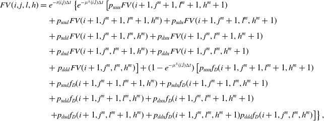 \begin{align} FV(i,j,l,h) & = e^{-r(i,j)\Delta t}\left\{e^{-\mu^x(i,l)\Delta t}\left[p_{uuu}FV(i+1,j^m+1,l^m+1,h^m+1)\right.\right.\nonumber\\[4pt]& \quad +p_{uud}FV(i+1,j^m+1,l^m+1,h^m)+p_{udu}FV(i+1,j^m+1,l^m,h^m+1) \nonumber\\[4pt]& \quad +p_{udd}FV(i+1,j^m+1,l^m,h^m)+p_{duu}FV(i+1,j^m,l^m+1,h^m+1) \nonumber\\[4pt]& \quad +p_{dud}FV(i+1,j^m,l^m+1,h^m)+p_{ddu}FV(i+1,j^m,l^m,h^m+1) \nonumber\\[4pt]& \quad +\left.p_{ddd}FV(i+1,j^m,l^m,h^m)\right]+(1-e^{-\mu^x(i,l)\Delta t}) \left[p_{uuu}f_D(i+1,j^m+1,l^m+1,h^m+1) \right.\nonumber\\[4pt]& \quad +p_{uud}f_D(i+1,j^m+1,l^m+1,h^m)+p_{udu}f_D(i+1,j^m+1,l^m,h^m+1) \nonumber\\[4pt]& \quad +p_{udd}f_D(i+1,j^m+1,l^m,h^m)+p_{duu}f_D(i+1,j^m,l^m+1,h^m+1) \nonumber\\[4pt]& \quad \left.\left. + p_{dud}f_D(i+1,j^m,l^m+1,h^m)+p_{ddu}f_D(i+1,j^m,l^m,h^m+1) p_{ddd}f_D(i+1,j^m,l^m,h^m)\right]\right\},\end{align}
while, whenever a surrender option is embedded in the endowment contract, the fair policy value in state of nature (i, j, l, h) is computed as the maximum between the quantity in the right-hand side of Equation (4.11) and the surrender value S(i, j, l, h).
5. Numerical results
In this section, we provide some numerical experiments supporting both the bivariate and the trivariate models presented above. Hereafter, we start each section by specifying the form of the processes considered for the interest rate, the mortality rate, and the equity. Then, we provide valuations for the contracts detailed in the previous sections. Clearly, other insurance contracts may be easily evaluated through the proposed models by making different choices of the process dynamics. Indeed, the following represents just a possible choice of the form assigned to processes (2.1), (2.2), and (2.3), but as already evidenced the model is able to work under any specification of the three processes among the ones commonly used in financial and actuarial markets.
5.1. Bond valuations through the bivariate model
To evaluate survival zero coupon bonds and mortality bonds, we specify the form of the dynamics characterizing the processes (2.1) and (2.2) as follows:
-
the r-process obeys to a Hull and White (Reference Hull and White1993) one-factor model with
$m_r(r_t)=\theta_r(t)-a(t)r_t$
and
$\sigma_r(r_t)=\sigma_r$
where, for the sake of simplicity and without loss of generality, we impose that
$\theta_r(t)$
and a(t) are positive constants, that is,
$\theta_r(t)=\theta_r$
and
$a(t)=a$
; -
the mortality
$\mu^x$
-process obeys to a Hull and White (Reference Hull and White1993) model with
$m_{\mu}(\mu^x_t)=\xi_{\mu}(t)-b(t)\mu^x_t$
and
$\sigma_{\mu}(\mu^x_t)=\sigma_{\mu}$
, where again we impose that
$\xi_{\mu}(t)$
and b(t) are positive constants, that is,
$\xi_{\mu}(t)=\xi_{\mu}$
and
$b(t)=b$
.


These choices relies on the fact that, under these conditions, it is possible to obtain an explicit solution to compute both the survival zero coupon bond price and the mortality bond price.
5.1.1. Survival zero coupon bonds
As in Hanna and Devolder (Reference Hanna and Devolder2023), the value at time t of a survival zero coupon bond paying one unit of money at maturity T is given by
 \begin{equation} B(t,T)=P(t,T){_{T-t}p}_{x+t}\rho(t,T),\end{equation}
where
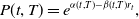 \begin{equation} P(t,T)=e^{\alpha(t,T)-\beta(t,T)r_t},\end{equation}
with
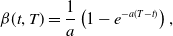 \begin{equation} \beta(t,T)=\frac{1}{a}\left(1-e^{-a(T-t)}\right),\end{equation}
and
 \begin{equation} \alpha(t,T)=\frac{(\beta(t,T)-T+t)(a\theta_r-0.5\sigma_r^2)}{a^2}-\frac{\sigma_r^2\beta^2(t,T)}{4a},\end{equation}
while
 \begin{equation} {_{T-t}p}_{x+t}=e^{\alpha'(t,T)-\beta'(t,T)\mu^x_t},\end{equation}
with
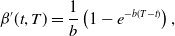 \begin{equation} \beta'(t,T)=\frac{1}{b}\left(1-e^{-b(T-t)}\right),\end{equation}
and
 \begin{equation} \alpha'(t,T)=\frac{(\beta'(t,T)-T+t)(b\xi_{\mu}-0.5\sigma_{\mu}^2)}{b^2}-\frac{\sigma_{\mu}^2\beta'^2(t,T)}{4b}.\end{equation}
Finally,
 \begin{equation} \rho(t,T)=e^{\frac{\sigma_r\sigma_{\mu}\rho_{12}}{ab}\left\{(T-t)-\frac{1-e^{-a(T-t)}}{a}-\frac{1-e^{-b(T-t)}}{b}+\frac{1-e^{-(a+b)(T-t)}}{a+b}\right\}}.\end{equation}
Using the results provided by formula (5.1) as the benchmark, we assess the accuracy of the results computed through the bivariate model and, then, conduct an analysis to show the effect of mortality on bond prices when varying the correlation coefficient value $\rho_{12}$
. In detail, in Table 1, we report the fair value at time
$\rho_{12}$
. In detail, in Table 1, we report the fair value at time $t=0$
of a bond paying one unit of money at time T, when varying T and the correlation value
$t=0$
of a bond paying one unit of money at time T, when varying T and the correlation value $\rho_{12}$
. The other parameter values are set up as:
$\rho_{12}$
. The other parameter values are set up as: $r_0=0.04$
,
$r_0=0.04$
, $\theta_r=0.04$
,
$\theta_r=0.04$
, $a=0.03$
,
$a=0.03$
, $\sigma_r=0.1$
,
$\sigma_r=0.1$
, $\mu^x_0=0.02$
,
$\mu^x_0=0.02$
, $\xi_{\mu}=0.02$
,
$\xi_{\mu}=0.02$
, $b=1.5$
, and
$b=1.5$
, and $\sigma_{\mu}=0.2$
. The first row reports, for each case, the value computed by the bivariate model (BM) when the number of time steps is fixed to
$\sigma_{\mu}=0.2$
. The first row reports, for each case, the value computed by the bivariate model (BM) when the number of time steps is fixed to $n=2000$
, while the second row reports the fair bond value computed by the explicit formula (5.1) (Exp.).
$n=2000$
, while the second row reports the fair bond value computed by the explicit formula (5.1) (Exp.).
Table 1. Fair survival bond values.
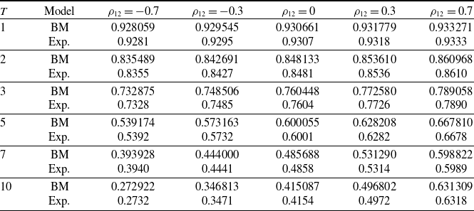
In Table 1, it is worth noting the accuracy of the results provided by the bivariate approximation with respect to the benchmark explicit values in all the analysed cases and the drastic effect of the correlation coefficient on the fair bond value. Clearly, this effect is more evident when increasing the bond maturity T and certifies how an accurate valuation of a product when embedding the mortality risk needs to be conducted taking properly into account the correlation insisting between financial and actuarial risks, that is, interest rate risk and mortality risk. To further show this evidence, in Figures 2 and 3, we show the correlation impact when varying $\rho_{12}\in[-1,1]$
and T from 1 year to 5 years in Figure 2 and from 6 years to 10 years in Figure 3. Both the figures confirm that an accurate determination of the correlation characterizing the two processes is absolutely requested in order to provide accurate fair bond value evaluations. Indeed, varying
$\rho_{12}\in[-1,1]$
and T from 1 year to 5 years in Figure 2 and from 6 years to 10 years in Figure 3. Both the figures confirm that an accurate determination of the correlation characterizing the two processes is absolutely requested in order to provide accurate fair bond value evaluations. Indeed, varying $\rho_{12}$
the fair bond value changes substantially and this effect is greater and greater when increasing the bond time to maturity T.
$\rho_{12}$
the fair bond value changes substantially and this effect is greater and greater when increasing the bond time to maturity T.

Figure 2. Fair bond values when varying $\rho_{12}\in[-1,1]$
and
$\rho_{12}\in[-1,1]$
and $T\in[1,5]$
.
$T\in[1,5]$
.
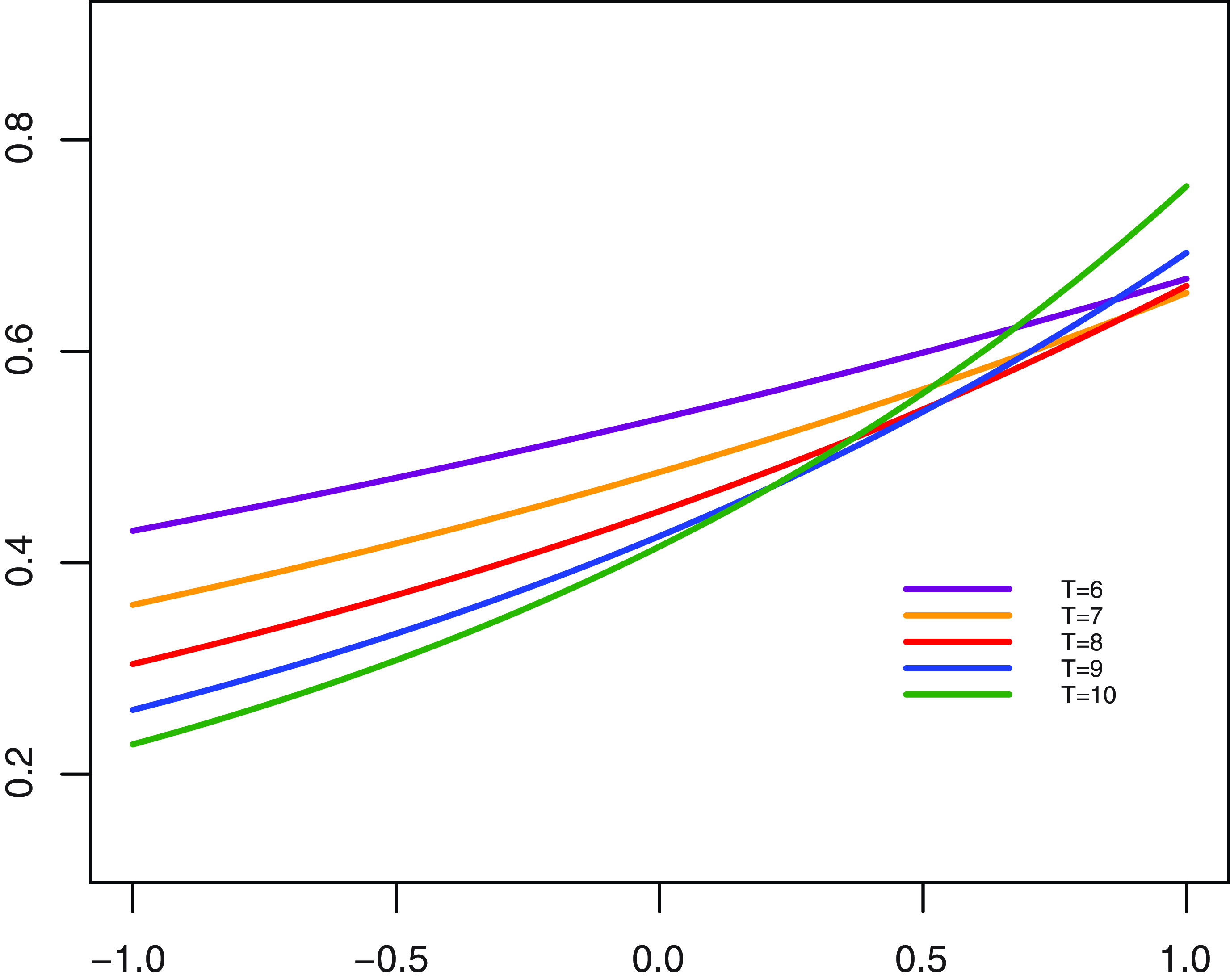
Figure 3. Fair bond values when varying $\rho_{12}\in[-1,1]$
and
$\rho_{12}\in[-1,1]$
and $T\in[6,10]$
.
$T\in[6,10]$
.
In Table 2, we provide a numerical analysis in order to show the convergence of the proposed bivariate model. In detail, we consider two cases already analysed in Table 1 in correspondence of $T=1$
and
$T=1$
and $\rho=-0.7$
, and of
$\rho=-0.7$
, and of $T=10$
and
$T=10$
and $\rho=0.7$
, and report the convergence pattern followed by the survival zero coupon bond values when doubling the number of time steps in the bivariate model. In the column “Difference”, we report the difference between two consecutive bond values, while in the column “Ratio” we report the ratio between two consecutive differences. It is worth evidencing that in both cases the ratios are closed to 0.5, the absolute value of the differences is about halved and the changes in bond values tend to zero when doubling the number of time steps, thus confirming the convergent behaviour of the values supplied by the bivariate model.
$\rho=0.7$
, and report the convergence pattern followed by the survival zero coupon bond values when doubling the number of time steps in the bivariate model. In the column “Difference”, we report the difference between two consecutive bond values, while in the column “Ratio” we report the ratio between two consecutive differences. It is worth evidencing that in both cases the ratios are closed to 0.5, the absolute value of the differences is about halved and the changes in bond values tend to zero when doubling the number of time steps, thus confirming the convergent behaviour of the values supplied by the bivariate model.
Table 2. Convergence patterns of the survival zero coupon bond values.
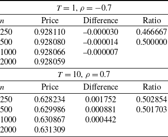
5.1.2. Mortality bonds
An explicit solution is also obtainable for the mortality bond characterized by traditional fixed coupons yearly payed and a principal at maturity becoming random and linked with realized longevity or mortality experiences. Denoting by T the maturity of the bond, c the fixed coupons and L(T) the stochastic principal, the price at time t (we impose $t<1$
to give consistency to the contract) of the instrument is given by
$t<1$
to give consistency to the contract) of the instrument is given by
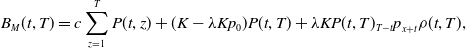 \begin{equation} B_{M}(t,T)=c\sum\limits_{z=1}^{T}P(t,z)+(K-\lambda K p_0) P(t,T)+\lambda K P(t,T){_{T-t}p}_{x+t}\rho(t,T),\end{equation}
where the involved quantities have been already defined above in Equations (5.2)–(5.8). The results provided by formula (5.9) are used as benchmark values to assess the accuracy of the results computed through the bivariate model for the mortality bond. In detail, in Table 3, we report the fair value at time $t=0$
of a mortality bond maturing at time T, when varying T and the correlation value
$t=0$
of a mortality bond maturing at time T, when varying T and the correlation value $\rho_{12}$
. We define the initial value of the survival probability as
$\rho_{12}$
. We define the initial value of the survival probability as $p_0=e^{-\mu^x_0T}$
and set up the other parameter values as:
$p_0=e^{-\mu^x_0T}$
and set up the other parameter values as: $r_0=0.04$
,
$r_0=0.04$
, $\theta_r=0.04$
,
$\theta_r=0.04$
, $a=0.03$
,
$a=0.03$
, $\sigma_r=0.1$
,
$\sigma_r=0.1$
, $\mu^x_0=0.02$
,
$\mu^x_0=0.02$
, $\xi_{\mu}=0.02$
,
$\xi_{\mu}=0.02$
, $b=1.5$
,
$b=1.5$
, $\sigma_{\mu}=0.2$
,
$\sigma_{\mu}=0.2$
, $K=100$
,
$K=100$
, $c=2$
, and
$c=2$
, and $\lambda=0.5$
. The first row reports, for each case, the value computed by the bivariate model (BM) when the number of time steps is fixed to
$\lambda=0.5$
. The first row reports, for each case, the value computed by the bivariate model (BM) when the number of time steps is fixed to $n=2000$
, while the second row reports the fair bond value computed by the explicit formula (5.9) (Exp.). Similarly to Table 1, Table 3 confirms the accuracy of the results provided by the bivariate approximation with respect to the benchmark explicit values in all the analysed cases and the drastic effect of the correlation coefficient on the fair mortality bond value.
$n=2000$
, while the second row reports the fair bond value computed by the explicit formula (5.9) (Exp.). Similarly to Table 1, Table 3 confirms the accuracy of the results provided by the bivariate approximation with respect to the benchmark explicit values in all the analysed cases and the drastic effect of the correlation coefficient on the fair mortality bond value.
In Table 4, we provide a numerical analysis to show the convergence of the mortality bond values that is similar to the one proposed in Table 2. Again, we consider two cases already analysed in Table 3 in correspondence of $T=2$
and
$T=2$
and $\rho=-0.7$
, and of
$\rho=-0.7$
, and of $T=10$
and
$T=10$
and $\rho=0.7$
, and show the convergence pattern followed by the mortality bond values when doubling the number of time steps in the bivariate model. As before, in both cases, the ratios are closed to 0.5, the absolute value of the differences is about halved and the changes in bond values tend to zero when doubling the number of time steps, thus confirming the convergent behaviour of the values supplied by the bivariate model.
$\rho=0.7$
, and show the convergence pattern followed by the mortality bond values when doubling the number of time steps in the bivariate model. As before, in both cases, the ratios are closed to 0.5, the absolute value of the differences is about halved and the changes in bond values tend to zero when doubling the number of time steps, thus confirming the convergent behaviour of the values supplied by the bivariate model.
Table 3. Fair mortality bond values.
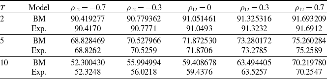
Table 4. Convergence patterns of the mortality bond values.
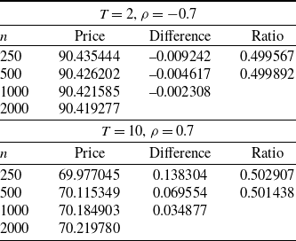
5.2. Equity-linked policy valuations through the trivariate model
To provide some numerical experiments using the presented trivariate model, we specify the form of the dynamics characterizing the processes (2.1), (2.2), and (2.3) as detailed hereafter:
-
the r-process follows a Hull and White (Reference Hull and White1993) one-factor model with
$m_r(r_t)=\kappa_r(\theta_r(t)-a(t)r_t)$
and
$\sigma_r(r_t)=\sigma_r$
where, for the sake of simplicity and without loss of generality, we impose that
$\theta_r(t)$
and a(t) are positive constants, that is,
$\theta_r(t)=\theta_r$
and
$a(t)=a$
; -
the mortality
$\mu^x$
-process follows a Cox et al. (Reference Cox, Ingersoll and Ross1985) model with
$m_{\mu}(\mu^x_t)=\xi_{\mu}(t)-b\mu^x_t$
and
$\sigma_{\mu}(\mu^x_t)=\sigma_{\mu}\sqrt{\mu^x_t}$
, where
$\xi_{\mu}(t)$
obeys to a Gompertz law of the form
$\xi_{\mu}(t)=Ae^{Bt}$
, with A and B positive constants; -
the equity S-process follows a Black-Scholes dynamics with
$m_S(r_t,S_t)=r_tS_t$
and
$\sigma_S(S_t)=\sigma_S S_t$
.


The numerical experiments aim at assessing the goodness of the proposed model and its applicability for valuing different insurance policies. We analyse insurance policies with or without embedding a surrender option in the policy contract in order to show the flexibility of the model and also consider different correlation structures among the three processes in order to show their impact on the policy values. To further support the numerical findings, in absence of the surrender option, we develop a Monte Carlo method assumed to be the benchmark. All the Monte Carlo simulations used to generate the results reported in this section are based on 400 observations and 100,000 trajectories.
In Table 5, we consider an equity-linked term policy with different times to maturity and provide a comparison with Monte Carlo simulations, when we do not embed in the policy contract the possibility for early surrender (No surr.). Whenever a surrender option is embedded in the policy contract, we define the surrender value in each state of nature as $SV(i,j,l,h)=\max\left[S(i,h),G\right]$
and report the corresponding policy value in the second column (Surr.) of each analysed case. We report the fair value at time
$SV(i,j,l,h)=\max\left[S(i,h),G\right]$
and report the corresponding policy value in the second column (Surr.) of each analysed case. We report the fair value at time $t=0$
of a policy maturing at time T, computed by the trivariate model (TM) with
$t=0$
of a policy maturing at time T, computed by the trivariate model (TM) with $n=400$
and the Monte Carlo (MC) simulations (standard errors (SE) are reported in brackets) when varying T and the correlation values
$n=400$
and the Monte Carlo (MC) simulations (standard errors (SE) are reported in brackets) when varying T and the correlation values $\rho_{12}$
,
$\rho_{12}$
, $\rho_{13}$
, and
$\rho_{13}$
, and $\rho_{23}$
. The other parameter values are set up as:
$\rho_{23}$
. The other parameter values are set up as: $r_0=0.04$
,
$r_0=0.04$
, $\theta_r=0.04$
,
$\theta_r=0.04$
, $a=0.03$
,
$a=0.03$
, $\sigma_r=0.01$
,
$\sigma_r=0.01$
, $\mu^x_0=0.02$
,
$\mu^x_0=0.02$
, $b=0.1$
,
$b=0.1$
, $\sigma_{\mu}=0.05$
,
$\sigma_{\mu}=0.05$
, $A=0.002$
,
$A=0.002$
, $B=0.001$
,
$B=0.001$
, $S_0=100$
,
$S_0=100$
, $\sigma_S=0.1358$
.
$\sigma_S=0.1358$
.
Table 5. Fair values of term policies.
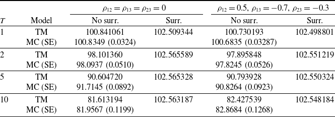
The results reported in Table 5 show the accuracy of the policy values computed by the proposed trivariate model with respect to the Monte Carlo benchmark values in absence of the surrender option. When introducing the surrender option, the policy contract assumes the feature of an American-style derivative that the trivariate model is able to manage and provides greater values with respect to the no-surrender case, as expected. We do not implement a least square Monte Carlo method since it is very complex to realize due to the presence of three different processes and very time consuming, while the proposed model is of straightforward application. This aspect supports further the algorithm flexibility of application.
In Table 6, we provide results for an equity-linked endowment policy using the same parameters of Table 5. We still consider both cases, with and without surrender options, define the surrender value in each state of nature as $SV(i,j,l,h)=\max\left[S(i,h),G\right]$
, and in addition we define by
$SV(i,j,l,h)=\max\left[S(i,h),G\right]$
, and in addition we define by $f_D(i,j,l,h)=G$
the amount paid to the policyholder in case of death, as already specified in Section 4.2.
$f_D(i,j,l,h)=G$
the amount paid to the policyholder in case of death, as already specified in Section 4.2.
In this case too, the results provided by the trivariate model are really close to the ones generated by the Monte Carlo simulations in absence of the surrender option, while they are greater with respect to the no-surrender case when embedding a surrender option, as expected.
In Table 7, we provide a numerical analysis in order to show the convergence of the trivariate model. In detail, we analyse the two cases reported in Tables 5 and 6 in correspondence of $T=1$
and
$T=1$
and $\rho_{12}=0.5$
,
$\rho_{12}=0.5$
, $\rho_{13}=-0.7$
,
$\rho_{13}=-0.7$
, $\rho_{23}=-0.3$
, in absence of the surrender option. For both cases, we show the convergence pattern followed by equity-linked policy values when doubling the number of time steps in the trivariate model. Again, the column “Difference” shows the difference between two consecutive policy values, while the column “Ratio” shows the ratio between two consecutive differences. In both analysed cases, the ratios are closed to 0.5, the absolute value of the differences is about halved and the changes in equity-linked policy values tend to zero when doubling the number of time steps, thus confirming the convergent behaviour of the values supplied by the trivariate model, too.
$\rho_{23}=-0.3$
, in absence of the surrender option. For both cases, we show the convergence pattern followed by equity-linked policy values when doubling the number of time steps in the trivariate model. Again, the column “Difference” shows the difference between two consecutive policy values, while the column “Ratio” shows the ratio between two consecutive differences. In both analysed cases, the ratios are closed to 0.5, the absolute value of the differences is about halved and the changes in equity-linked policy values tend to zero when doubling the number of time steps, thus confirming the convergent behaviour of the values supplied by the trivariate model, too.
Table 6. Fair values of endowment policies.
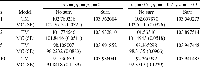
Table 7. Convergence patterns of the equity-linked policy values.
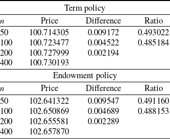
6. Conclusions
The paper proposes a lattice-based model that is able to combine financial and actuarial aspects when valuing insurance policies. Indeed, all sources of risks are managed in the proposed framework where interest rate, mortality, and equity dynamics move stochastically. An appealing feature of the model is its flexibility that relies on its ability to manage different specifications of the three processes, thus allowing the insurer to make the most appropriate choices concerning the dynamics to be used. The model is also able to handle additional guarantees like a surrender opportunity. On a methodological point of view, the paper provides both a bivariate and a trivariate model. The first case, in which we combine the discretizations proposed for the interest and mortality rates, is useful to compute, for instance, the value of survival zero coupon bond. Introducing an additional source of risk as the fund dynamic in order to evaluate fund-linked insurance products, we obtain a trivariate tree presenting eight branches emanating from each node in which the joint probability of each jump is defined in order to capture the proper pairwise process correlation. Extensive numerical experiments assess the model accuracy by considering some stylized policies, but the model application is not limited to them being it able to manage different contract specifications.
Future works will be focused on the analysis of the extension of the proposed models to different evaluation environments for which they are not of straightforward application. We may refer, for instance, to the frameworks currently used to evaluate products affected by climate risk where climate risk impacts both actuarial and financial aspects, to mortality bonds with nonlinear loss functions generating path dependent payoff, or to models that consider the impact of the inflation on the valuation of actuarial or financial products and capture its dynamics along time through a stochastic process, inflation becoming then an additional correlated risk factor. The latter is also of great interest due to the current evolution of inflation rates that are affecting substantially the purchasing power of economic agents. Another aspect to look at is the possibility to speed up the convergence rates of the proposed discretizations by introducing in the algorithm an extrapolation method like the one proposed, among others, by Korn and Müller (Reference Korn and Müller2009).
Acknowledgements
Emilio Russo acknowledges co-funding from Next Generation EU, in the context of the National Recovery and Resilience Plan, Investment PE8 – Project Age-It: “Ageing Well in an Ageing Society”. This resource was co-financed by the Next Generation EU [DM 1557 11.10.2022]. The views and opinions expressed are only those of the authors and do not necessarily reflect those of the European Union or the European Commission. Neither the European Union nor the European Commission can be held responsible for them. Emilio Russo and Alessandro Staino acknowledge co-funding from the Italian Ministry of University and Research, PRIN 2022 – Project number 2022FWZ2CR: “Building resilience to emerging risks in financial and insurance markets”. This resource was co-financed by the Italian Ministry of University and Research [DD 967 30.06.2023].
Competing interests
The authors declare none.
Appendix
As evidenced in Sections 2.2 and 2.3, both the lattices for the r-process and the $\mu$
-process follow a similar construction that starts from the definition of the values for the nodes on the edges and, then, obtains the values for the inner nodes by generating horizontal layers of nodes starting from the nodes located on the two edges. Hence, we limit to prove that
$\mu$
-process follow a similar construction that starts from the definition of the values for the nodes on the edges and, then, obtains the values for the inner nodes by generating horizontal layers of nodes starting from the nodes located on the two edges. Hence, we limit to prove that $p_r(i,j)\rightarrow \frac{1}{2}$
as
$p_r(i,j)\rightarrow \frac{1}{2}$
as $n\rightarrow +\infty$
because similarly we may prove that
$n\rightarrow +\infty$
because similarly we may prove that $p_{\mu}(i,l)\rightarrow \frac{1}{2}$
as
$p_{\mu}(i,l)\rightarrow \frac{1}{2}$
as $n\rightarrow +\infty$
. To prove that
$n\rightarrow +\infty$
. To prove that $p_r(i,j)\rightarrow \frac{1}{2}$
as
$p_r(i,j)\rightarrow \frac{1}{2}$
as $n\rightarrow +\infty$
, it is equivalent to prove that the probability of an upward movement starting from a node of the lattice edge (i.e., node
$n\rightarrow +\infty$
, it is equivalent to prove that the probability of an upward movement starting from a node of the lattice edge (i.e., node $(i,i),i=0,\ldots,n$
) tends to
$(i,i),i=0,\ldots,n$
) tends to $\frac{1}{2}$
because the inner node values replicate the values on the edges. To simplify matters, we suppose that no multiple jumps occur so that, by considering a node (i, i) on the highest edge, the successors bracketing the process expected value, that is,
$\frac{1}{2}$
because the inner node values replicate the values on the edges. To simplify matters, we suppose that no multiple jumps occur so that, by considering a node (i, i) on the highest edge, the successors bracketing the process expected value, that is, $r(i,j)+m_r(r(i,i))\Delta t$
, are
$r(i,j)+m_r(r(i,i))\Delta t$
, are $r(i+1,i+1)$
and
$r(i+1,i+1)$
and $r(i+1,i)$
. Due to the proposed construction, their value coincide with
$r(i+1,i)$
. Due to the proposed construction, their value coincide with $r(i+1,i+1)=r(i,i)+\sigma_r(r(i,i))\sqrt{\Delta t}$
, because it is still on the upper edge, and
$r(i+1,i+1)=r(i,i)+\sigma_r(r(i,i))\sqrt{\Delta t}$
, because it is still on the upper edge, and $r(i+1,i)=r(i-1,i-1)$
, being it an inner lattice node. Applying formula (2.4), we can compute the probability of an upward movement as follows:
$r(i+1,i)=r(i-1,i-1)$
, being it an inner lattice node. Applying formula (2.4), we can compute the probability of an upward movement as follows:
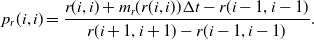 \begin{equation} p_r(i,i) = \frac{r(i, i)+m_r(r(i,i))\Delta t - r(i - 1,i-1)}{r(i + 1, i + 1) -r(i - 1, i-1)}.\end{equation}
Recalling that by construction we have $r(i+1,i+1)=r(i,i)+\sigma_r(r(i,i))\sqrt{\Delta t}$
and, similarly,
$r(i+1,i+1)=r(i,i)+\sigma_r(r(i,i))\sqrt{\Delta t}$
and, similarly, $r(i,i)=r(i-1,i-1)+\sigma_r(r(i-1,i-1))\sqrt{\Delta t}$
, we may also obtain
$r(i,i)=r(i-1,i-1)+\sigma_r(r(i-1,i-1))\sqrt{\Delta t}$
, we may also obtain $r(i+1,i+1)$
as a function of
$r(i+1,i+1)$
as a function of $r(i-1,i-1)$
, that is, the value on the lattice edge two steps before:
$r(i-1,i-1)$
, that is, the value on the lattice edge two steps before:
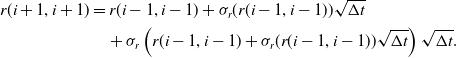 \begin{align*}r(i+1,i+1) & =r(i-1,i-1)+\sigma_r(r(i-1,i-1))\sqrt{\Delta t}\\& \quad +\sigma_r\left(r(i-1,i-1)+\sigma_r(r(i-1,i-1))\sqrt{\Delta t}\right)\sqrt{\Delta t}.\nonumber\end{align*}
By substituting in formula (A1) the values of $r(i+1,i+1)$
and r(i, i) written above as a function of
$r(i+1,i+1)$
and r(i, i) written above as a function of $r(i-1,i-1)$
and by a little algebra, we may obtain
$r(i-1,i-1)$
and by a little algebra, we may obtain $p_r(i,i)$
as the sum of two addenda as showed hereafter:
$p_r(i,i)$
as the sum of two addenda as showed hereafter:
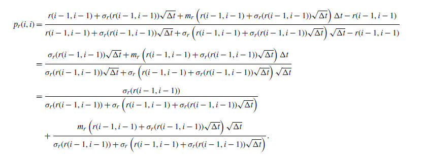 \begin{align*} p_r(i,i) & = \frac{r(i-1,i-1)+\sigma_r(r(i-1,i-1))\sqrt{\Delta t}+m_r\left(r(i-1,i-1)+\sigma_r(r(i-1,i-1))\sqrt{\Delta t}\right)\Delta t - r(i - 1,i-1)}{r(i-1,i-1)+\sigma_r(r(i-1,i-1))\sqrt{\Delta t}+\sigma_r\left(r(i-1,i-1)+\sigma_r(r(i-1,i-1))\sqrt{\Delta t}\right)\sqrt{\Delta t} -r(i - 1, i-1)}\nonumber\\[4pt]& = \frac{\sigma_r(r(i-1,i-1))\sqrt{\Delta t}+m_r\left(r(i-1,i-1)+\sigma_r(r(i-1,i-1))\sqrt{\Delta t}\right)\Delta t}{\sigma_r(r(i-1,i-1))\sqrt{\Delta t}+\sigma_r\left(r(i-1,i-1)+\sigma_r(r(i-1,i-1))\sqrt{\Delta t}\right)\sqrt{\Delta t} }\nonumber\\[4pt]& =\frac{\sigma_r(r(i-1,i-1))}{\sigma_r(r(i-1,i-1))+\sigma_r\left(r(i-1,i-1)+\sigma_r(r(i-1,i-1))\sqrt{\Delta t}\right)}\nonumber\\[4pt]& \quad +\frac{m_r\left(r(i-1,i-1)+\sigma_r(r(i-1,i-1))\sqrt{\Delta t}\right)\sqrt{\Delta t}}{\sigma_r(r(i-1,i-1))+\sigma_r\left(r(i-1,i-1)+\sigma_r(r(i-1,i-1))\sqrt{\Delta t}\right) }.\nonumber\end{align*}
When $n\rightarrow +\infty$
,
$n\rightarrow +\infty$
, $\Delta t \rightarrow 0$
so that the first addendum tends to
$\Delta t \rightarrow 0$
so that the first addendum tends to $\frac{1}{2}$
, the second addendum tends to 0 under the condition that the process drift and diffusion are finite, and to sum up
$\frac{1}{2}$
, the second addendum tends to 0 under the condition that the process drift and diffusion are finite, and to sum up $p_r(i,j)\rightarrow \frac{1}{2}$
.
$p_r(i,j)\rightarrow \frac{1}{2}$
.


 Open access