


1. Introduction
Pension buyout deals provide an attractive solution for defined benefit (DB) pension schemes to immediately discharge their liabilities by transferring all risks to an insurer or other financial agent (Blake et al., Reference Blake, Cairns, Coughlan, Dowd and MacMinn2013; Lin et al., Reference Lin, MacMinn and Tian2015). While such deals require the pension fund to pay an upfront fee to the insurer, all unexpected future changes to interest rates, mortality rates and other risk factors are then borne by the insurer. From the buyout insurer’s point of view, these transactions can be very advantageous by providing an opportunity to earn attractive returns from capital markets based on their expertise in asset and liability management (Biffis and Blake, Reference Biffis and Blake2009). From the DB pension schemes’ point of view, pension buyouts provide more freedom, allowing the DB plan sponsors to take on more risky projects with high positive net present values. This creates added value compared to other financial contracts that can be used to hedge annuities, such as longevity swaps (Cox et al., Reference Cox, Lin and Shi2018).
The vast majority of the existing literature on pension buyouts has focused on understanding the philosophy of such deals and the newly emerged pension bulk annuity market. For instance, Monk (Reference Monk2009) complements the previous works of Kirkpatrick (Reference Kirkpatrick2007) and Blake et al. (Reference Blake, Cairns and Dowd2008) by evaluating the pension bulk annuity market in the UK and then analyses its implications for the USA. Moreover, buyout deals are investigated as a transaction for both insolvent and solvent plans in the same study. Biffis and Blake (Reference Biffis and Blake2013) analyse pension buyouts and longevity securitisation in the same context and develop a coherent model of intermediation of longevity exposures between DB plans and capital markets. Furthermore, Biffis and Blake (Reference Biffis and Blake2014) discuss a natural way for longevity risk to be transferred to the capital markets and evaluate buyout firms in this context as ‘aggregators of the pension liabilities of small companies into larger pools’. To the best of our knowledge, the study of Lin et al. (Reference Lin, Shi and Arik2017) is the first published work on pricing pension buy-ins and buyouts. They develop a benchmark pricing model for both pension buy-ins and buyouts under the independence assumption between financial and insurance markets. Furthermore, Cox et al. (Reference Cox, Lin and Shi2018) investigate how to make pension buyout contracts more affordable for underfunded DB plans as these contracts can be very expensive when the pension fund runs a deficit. Arik et al. (Reference Arik, Yolcu-Okur, Şahin and Uğur2018) investigate pricing pension buyouts by considering a specific dependence structure between mortality and interest rate risk.
In this study, we focus on pension buyout and life annuity prices assuming that mortality rates and financial markets are not independent. In particular, we are interested in how a pandemic, such as COVID-19, that simultaneously causes unexpected high mortality and increased uncertainty in the global economy, may affect buyout and annuity prices. We examine buyout prices for a hypothetical population based on an extensive simulation analysis with the aim to shed some light on the uncertainty over future (bulk annuity) market valuations (Rothesay, 2022). Our analysis is centred around the question how prices are influenced by simultaneous shocks to mortality and financial markets as opposed to independent shocks. To cover a variety of market conditions, we run our simulation studies with a wide range of parameter values. The set-up also takes into account that we are pricing long-term products with annual payments. Assuming that shocks take place simultaneously in mortality and financial markets is clearly an approximation as the reaction of financial markets to changes in mortality might be delayed, and, of course, shocks to mortality might develop over the space of several weeks. However, we argue that the long-term nature of the contract considered in this paper justifies approximating the exact timing of a mortality shock and the market reaction to it by a simultaneous shock. For short-term financial products with a maturity of a few months rather than several years, a detailed empirical analysis of the timing of market reaction to mortality shocks would be crucial.
We use the pricing framework for pension buyouts developed by Arik et al. (Reference Arik, Yolcu-Okur, Şahin and Uğur2018) with some significant modifications: (i) we consider a different dependence structure between mortality rates and financial markets by assuming common shocks rather than a common Wiener process driving the risk processes – Section 1.1 has a detailed discussion of the independence assumption, (ii) we propose a jump diffusion model to describe the evolution of mortality rates with upward shocks and assume that the jumps in this model also affect financial markets and, finally, (iii) financial markets are assumed to be impacted via shocks to the short rates or asset returns. We also modify the numerical implementation of the buyout pricing formula to effectively deal with the required nested simulations.
With this paper, we aim to investigate the net effect that the shocks have on annuities and buyout prices. To investigate the effect of different factors, we run a large number of simulations with very different settings. Our findings indicate that while the independence assumption might be questionable, see Section 1.1, the impact on prices is rather limited – independent shocks seem to result in similar buyout prices as simultaneous shocks. The greatest impact on buyout prices is coming from asset price volatility, see Section 5 for details.
The remainder of this paper is organised as follows. After discussing the independence assumption in Section 1.1, we explain the models for mortality and short rate dynamics in Section 2, and then we show how to derive the price of a pension buyout deal in Section 3. In Section 4, we explain how to carry out nested simulations to obtain life annuity prices. In Section 5, we present the applicability of the proposed approach using three main scenarios. Section 6 concludes the paper.
1.1 The (in-)dependence assumption and empirical relevance of this study
The independence assumption between financial and mortality risks is very convenient as it allows for pricing the risks independently of each other. After all, it is helpful when the expectation of a product is the product of the expectations. However, this is a very strong assumption which should come with strong justification. While this assumption might be intuitive to some extend under the real-world (or empirical) measure, it is questionable whether it still holds under the pricing measure. Dhaene et al. (Reference Dhaene, Kukush, Luciano, Schoutens and Stassen2013) provide a beautiful and detailed discussion of this issue including a very simple example for a financial–biometrical market where the independence assumption holds under the real-world measure but not under the risk-neutral pricing measure.
Furthermore, the appropriateness of the real-world independence assumption is also challenged in several published studies including Ruhm (Reference Ruhm2000), Brainerd and Siegler (Reference Brainerd and Siegler2003), Nicolini (Reference Nicolini2004), Tapia Granados (Reference Tapia Granados2005), Jonung and Roeger (Reference Jonung and Roeger2006), Burns et al. (Reference Burns, Mensbrugghe and Timmer2008), Riberio and Pietro (Reference Riberio and Pietro2009), Jalen and Mamon (Reference Jalen and Mamon2009), Hanewald (Reference Hanewald2011), Liu et al. (Reference Liu, Mamon and Gao2014), Dacorogna and Cadena (Reference Dacorogna and Cadena2015), Aro and Pennanen (Reference Aro and Pennanen2014) and Seklecka et al. (Reference Seklecka, Lazam, Pantelous and O’Hare2019). For instance, Jalen and Mamon (Reference Jalen and Mamon2009) state that ‘in the long run, interest rates can be influenced by the relative size of the population, which in turn, is influenced by mortality development (as well as fertility)’, and ‘in the short term, a catastrophic event that seriously affects the size of the population, such as major natural disasters or a nuclear war, can also affect interest rates’. It is worth to note that empirical studies suggest a weak (negative) correlation, for example 10–20%, between the changes in mortality rates and financial markets in normal times, but strong dependency as a result of extreme changes in mortality, for example, a severe drop in equity returns as
 $-4.57$
% where the average return is 4.87% (Jonung and Roeger, Reference Jonung and Roeger2006; Riberio and Pietro, Reference Riberio and Pietro2009; Dacorogna and Cadena, Reference Dacorogna and Cadena2015).
$-4.57$
% where the average return is 4.87% (Jonung and Roeger, Reference Jonung and Roeger2006; Riberio and Pietro, Reference Riberio and Pietro2009; Dacorogna and Cadena, Reference Dacorogna and Cadena2015).
The relationship between financial and biometrical risks is further complicated by risk perception. For instance, the ‘risks-as-feelings hypothesis’ indicates that feelings are the main drivers of decision-making mechanisms, and background mood or feelings could impact the assessment of risky decisions (Johnson and Tversky, Reference Johnson and Tversky1983 Loewenstein et al., Reference Loewenstein, Weber, Hsee and Welch2001; Nofsinger, Reference Nofsinger2005). In behavioural finance, it is argued that the social mood can affect the stock market – for example, suicide rates are argued to impact the financial markets (negatively) (Nofsinger, Reference Nofsinger2005; Choi, Reference Choi2016).
In early 2020, we observed that capital markets were falling due to uncertainty related to the effect of the COVID-19 pandemic on the global economy and stock markets. For instance, the Shanghai and Hang Seng indexes fell, around 6–8%, between January and March 2020. At the same time, it started to become clear to investors around the globe that mortality from this new virus is very high. For example, the observed total mortality in Wuhan city between 1 January and 31 March 2020 was reported to be significantly higher, 56%, as compared to the same period in 2019 (Liu et al., Reference Liu, Zhang, Yan, Zhou, Yin, Qi, Wang, Pan, You, Yang, Zhao, Wang, Liu, Lin, Wu, Li, Chen and Zhou2021). Also, the three main US indexes, the S&P 500, Nasdaq and Dow Jones, fell sharply, around 10%, in a week in February 2020, suffering the worst week since the financial crisis of 2008 while the UK’s FTSE 100 share index dropped 3.3% (Hussain, Reference Hussain2020; David, Reference David2020). While financial markets recovered, economic uncertainty continued throughout the years 2020 and 2021.
This discussion leads us to the conclusion that the independence assumption is questionable. Therefore, we assume in this paper that upward shocks in mortality rates have an impact on financial markets, leading to decreasing interest rates or asset returns (Jalen and Mamon, Reference Jalen and Mamon2009; Liu et al., Reference Liu, Zhang, Yan, Zhou, Yin, Qi, Wang, Pan, You, Yang, Zhao, Wang, Liu, Lin, Wu, Li, Chen and Zhou2021).
2. Modelling framework
In this section, we provide an overview of the continuous time models we use for mortality rates, interest rates and asset prices. Throughout the remainder of this paper, let
 $(\Omega,\mathcal{I}, \mathcal{I}_t, \mathbb{Q})$
be a probability space equipped with a filtration
$(\Omega,\mathcal{I}, \mathcal{I}_t, \mathbb{Q})$
be a probability space equipped with a filtration
 $\mathcal{I}_t$
. This probability space represents our combined modelling framework for mortality rates and financial market, and, in particular, the
$\mathcal{I}_t$
. This probability space represents our combined modelling framework for mortality rates and financial market, and, in particular, the
 $\sigma$
-algebra
$\sigma$
-algebra
 $\mathcal{I}_t$
represents the information up to time t generated by the joint evolution of mortality rates and financial markets.
$\mathcal{I}_t$
represents the information up to time t generated by the joint evolution of mortality rates and financial markets.
Since this paper is concerned with risk-neutral pricing of buyout contracts and annuities, we will describe the three parts of our model – mortality, interest rates and asset prices – under the risk-neutral pricing measure
 $\mathbb{Q}$
. This means in particular that all discounted price processes are
$\mathbb{Q}$
. This means in particular that all discounted price processes are
 $\mathbb{Q}$
-martingales. As we will choose mortality parameters based on observed mortality rates and the intensity of jumps based on the observed frequency of mortality shocks, this means that we assume that mortality dynamics are the same under the real-world measure
$\mathbb{Q}$
-martingales. As we will choose mortality parameters based on observed mortality rates and the intensity of jumps based on the observed frequency of mortality shocks, this means that we assume that mortality dynamics are the same under the real-world measure
 $\mathbb{P}$
and the pricing measure
$\mathbb{P}$
and the pricing measure
 $\mathbb{Q}$
. In other words, our pricing measure is a minimal entropy measure – we are choosing our pricing measure to be as close to the real-world measure as possible while making sure that all discounted price processes are
$\mathbb{Q}$
. In other words, our pricing measure is a minimal entropy measure – we are choosing our pricing measure to be as close to the real-world measure as possible while making sure that all discounted price processes are
 $\mathbb{Q}$
-martingales, see, for example, Dhaene et al. (Reference Dhaene, Stassen, Devolder and Vellekoop2015). This modelling choice is justified since we do not consider any traded mortality derivatives with observable market prices. Other choices of
$\mathbb{Q}$
-martingales, see, for example, Dhaene et al. (Reference Dhaene, Stassen, Devolder and Vellekoop2015). This modelling choice is justified since we do not consider any traded mortality derivatives with observable market prices. Other choices of
 $\mathbb{Q}$
would be possible, of course, but any such choice will always be subjective, see, for example, Dawson et al. (Reference Dawson, Dowd, Cairns and Blake2010), Zhou et al. (Reference Zhou, Li and Tan2013) and Bauer et al. (Reference Bauer, Börger and Ruß2010). Finally, risk-neutral valuation will be used to find annuity prices and buyout prices. Those prices are, therefore, discounted martingales under
$\mathbb{Q}$
would be possible, of course, but any such choice will always be subjective, see, for example, Dawson et al. (Reference Dawson, Dowd, Cairns and Blake2010), Zhou et al. (Reference Zhou, Li and Tan2013) and Bauer et al. (Reference Bauer, Börger and Ruß2010). Finally, risk-neutral valuation will be used to find annuity prices and buyout prices. Those prices are, therefore, discounted martingales under
 $\mathbb{Q}$
by construction which ensures that the financial market model is arbitrage free.
$\mathbb{Q}$
by construction which ensures that the financial market model is arbitrage free.
2.1 Modelling shocks
The key ingredient for our models is a pure jump process J that we use to model unexpected strong changes in mortality, interest rates or asset returns.
More precisely, in our model, J(t) is a compound Poisson process such that
 \begin{eqnarray*} J(t) = \sum_{i=1}^{N(t)}{ Y(i) },\end{eqnarray*}
where
 $\{N(t)\;:\;t \geq 0\}$
is a Poisson process with constant jump-arrival intensity
$\{N(t)\;:\;t \geq 0\}$
is a Poisson process with constant jump-arrival intensity
 $\lambda > 0$
under
$\lambda > 0$
under
 $\mathbb{Q}$
. The terms of the J(t) process,
$\mathbb{Q}$
. The terms of the J(t) process,
 $\{Y(i), \, i=1,2,3,\ldots\}$
, representing jump sizes, are assumed to be distributed exponentially with mean
$\{Y(i), \, i=1,2,3,\ldots\}$
, representing jump sizes, are assumed to be distributed exponentially with mean
 $j>0$
(Biffis, Reference Biffis2005). That means, at any jump time
$j>0$
(Biffis, Reference Biffis2005). That means, at any jump time
 $\tau >0$
, we have
$\tau >0$
, we have
 $ J(\tau) - J(\tau^-) \sim \mbox{Exp}(1/j)$
under
$ J(\tau) - J(\tau^-) \sim \mbox{Exp}(1/j)$
under
 $\mathbb{Q}$
.
$\mathbb{Q}$
.
2.2 Modelling mortality rates
For the mortality rate process, we consider a continuous time specification of the well-known LC model for the force of mortality,
 $\mu(t, x+t)$
, of a life aged x in year
$\mu(t, x+t)$
, of a life aged x in year
 $t=0$
:
$t=0$
:
 \begin{eqnarray} \mu(t, x+t) = \exp\big(\alpha(x+t) + \beta (x+t) \kappa(t) \big). \end{eqnarray}
In contrast to the original idea by Lee and Carter (Reference Lee and Carter1992), we model the period effect
 $\kappa(t)$
as a continuous time process, namely a Brownian motion with drift, following Protter (Reference Protter2004) and Biffis and Denuit (Reference Biffis and Denuit2006), that is,
$\kappa(t)$
as a continuous time process, namely a Brownian motion with drift, following Protter (Reference Protter2004) and Biffis and Denuit (Reference Biffis and Denuit2006), that is,
 \begin{eqnarray} d\kappa(t) = \delta_\kappa dt + \sigma_\kappa d W_\kappa(t). \end{eqnarray}
In light of the empirical findings mentioned in the introduction, we are particularly interested in upward jumps (unexpected high mortality rates) and therefore, we extend our model for the period effect to include a jump process that only allows for positive jumps:
 \begin{eqnarray} \mu(t, x+t) = \exp\bigg(\alpha(x+t) + \beta(x+t) \big( \kappa(t) + v_{\mu}\, J(t) \big) \bigg), \end{eqnarray}
where the jump process J(t), described in Section 2.1, is added to
 $\kappa$
and rescaled with the age-effect
$\kappa$
and rescaled with the age-effect
 $\beta(x+t)$
and a constant
$\beta(x+t)$
and a constant
 $v_{\mu}>0$
. Given that pandemics and other catastrophes would affect some ages more than others, the impact of jump process should be age-specific. In this setting,
$v_{\mu}>0$
. Given that pandemics and other catastrophes would affect some ages more than others, the impact of jump process should be age-specific. In this setting,
 $\beta(x+t)$
allows us to re-scale the jump process with respect to age in a natural manner.
$\beta(x+t)$
allows us to re-scale the jump process with respect to age in a natural manner.
For our simulation study, we will generate sample paths of mortality rates by first generating paths of the period effect
 $\kappa$
using a standard Euler scheme to approximate (2.3) such that
$\kappa$
using a standard Euler scheme to approximate (2.3) such that
 \begin{eqnarray}\kappa(t+{\Delta t}) = \kappa(t) + \delta_\kappa {\Delta t} + \sigma_\kappa {\Delta W}_{\kappa}(t),\end{eqnarray}
where
 ${\Delta W}_{\kappa}(t)=W_{\kappa}(t+{\Delta t}) - W_{\kappa}(t)$
are normally distributed with zero expectation and variance
${\Delta W}_{\kappa}(t)=W_{\kappa}(t+{\Delta t}) - W_{\kappa}(t)$
are normally distributed with zero expectation and variance
 ${\Delta t}$
. To generate mortality scenarios, we also require age effects at non-integer ages which we calculate from the age effects at integer ages with linear interpolation, that is,
${\Delta t}$
. To generate mortality scenarios, we also require age effects at non-integer ages which we calculate from the age effects at integer ages with linear interpolation, that is,
 \begin{eqnarray}\alpha(x+\Delta t) = ( 1 - \Delta t ) \alpha(x) + \Delta t \alpha( x + 1 ) \end{eqnarray}
 \begin{eqnarray} \beta(x+\Delta t) = ( 1 - \Delta t ) \beta(x) + \Delta t\beta( x + 1 ),\end{eqnarray}
for
 $0 < {\Delta t} <1$
. Finally, mortality scenarios at discrete times
$0 < {\Delta t} <1$
. Finally, mortality scenarios at discrete times
 $t = k \Delta t$
for
$t = k \Delta t$
for
 $k=1,2, \ldots$
are then generated using (2.3).
$k=1,2, \ldots$
are then generated using (2.3).
2.3 Modelling short rates
The dynamics of the short rates are governed by a Cox–Ingersoll–Ross (CIR) process defined on
 $(\Omega,\mathcal{I}, \mathcal{I}_t, \mathbb{Q})$
. Cox et al. (Reference Cox, Ingersoll and Ross1985) propose to model instantaneous short rate dynamics as follows:
$(\Omega,\mathcal{I}, \mathcal{I}_t, \mathbb{Q})$
. Cox et al. (Reference Cox, Ingersoll and Ross1985) propose to model instantaneous short rate dynamics as follows:
 \begin{eqnarray}dr(t) = \zeta (\theta - r(t) ) dt + \sigma_r \sqrt {r(t)} dW_r(t),\end{eqnarray}
where
 $\theta$
represents the long-term average short rate,
$\theta$
represents the long-term average short rate,
 $\zeta>0$
is the speed of adjustment (or speed of mean-reversion) and
$\zeta>0$
is the speed of adjustment (or speed of mean-reversion) and
 $\sigma_r>0$
is a constant that determines the volatility of the short rate. The process
$\sigma_r>0$
is a constant that determines the volatility of the short rate. The process
 $W_r$
is a standard Brownian motion under the measure
$W_r$
is a standard Brownian motion under the measure
 $\mathbb{Q}$
. We assume that the processes
$\mathbb{Q}$
. We assume that the processes
 $W^{\mu}$
,
$W^{\mu}$
,
 $W^{r}$
and J are independent under
$W^{r}$
and J are independent under
 $\mathbb{Q}$
.
$\mathbb{Q}$
.
We will consider a generalised version of the CIR model to reflect the (negative) influence of a pandemic or other mortality shocks on short rates:
 \begin{eqnarray} dr(t) = \zeta ( \theta - r(t) ) dt + \sigma_r \sqrt{r(t)} dW_r (t) - v_r dJ(t), \end{eqnarray}
such that the jump process J(t) is the same as we use in the mortality model, but it is rescaled with a different constant
 $ v_r >0$
.
$ v_r >0$
.
Note that having the same jump process J affecting mortality
 $\mu$
in (2.3) and the short rate r means that not only the timing of shocks is the same for both processes, but also the magnitudes are the same (up to the scaling constants
$\mu$
in (2.3) and the short rate r means that not only the timing of shocks is the same for both processes, but also the magnitudes are the same (up to the scaling constants
 $v_\mu$
and
$v_\mu$
and
 $v_r$
). We have chosen this approach for its simplicity but also for the fact that we believe a large shock to mortality will result in a large shock to interest rates. A more sophisticated way of modelling the jumps could allow for a more subtle relationship between them.
$v_r$
). We have chosen this approach for its simplicity but also for the fact that we believe a large shock to mortality will result in a large shock to interest rates. A more sophisticated way of modelling the jumps could allow for a more subtle relationship between them.
As our analysis is based on simulations, we replace
 $\sqrt{r(t)}$
in (2.8) with
$\sqrt{r(t)}$
in (2.8) with
 $\sqrt{|r(t)|}$
to deal with simulated negative values of r(t), that is,
$\sqrt{|r(t)|}$
to deal with simulated negative values of r(t), that is,
 \begin{equation}dr(t) = \zeta ( \theta - r(t) ) dt + \sigma_r \sqrt{ \vert{r(t)}\vert } dW_r (t) - v_r dJ(t).\end{equation}
This approach follows Higham and Mao (Reference Higham and Mao2005) and leads to a computationally safer version of the CIR model. Yet, (2.9) still holds the possibility of producing negative short rates which causes numerical problems and buyout premiums that do not reflect realistic market prices.
However, negative interest rate policies were introduced by several central banks, including the European Central Bank, in recent years, specifically since 2012 (Brandao-Marques et al., Reference Brandao-Marques, Casiraghi, Gelos, Kamber and Meeks2021). Also, overnight lending rates have been negative in the past, for example, the Euro OverNight Index Average, EONIA, realised around
 $-48$
% in June 2021 (ECB, 2021; EONIA, 2021). There are different estimates for a technical minimum for negative interest rates that reflect varying assumptions, such as storage, summarised in Table 1.
$-48$
% in June 2021 (ECB, 2021; EONIA, 2021). There are different estimates for a technical minimum for negative interest rates that reflect varying assumptions, such as storage, summarised in Table 1.
Table 1. Estimation of the effective lower bound for negative interest rates. Source: Brandao-Marques et al. (Reference Brandao-Marques, Casiraghi, Gelos, Kamber and Meeks2021).

In our simulation study, we discretise the expression for r in (2.8) to simulate short rate scenarios. Additionally, to allow for negative rates but avoid rates which we think are too low, we restrict the short rates to be bounded from below by a constant
 $r_b<0$
. Therefore, sample paths of the short rate process, r, are generated as follows:
$r_b<0$
. Therefore, sample paths of the short rate process, r, are generated as follows:
 \begin{eqnarray} r^0(t+{\Delta t}) &=& r(t) + \zeta \big( \theta - r(t) \big) {\Delta t} +\sigma_r \sqrt{\vert{ r(t)} \vert } \Big({\Delta W}_r(t)\Big) - v_r \Delta J(t) \nonumber \\[5pt] r(t+{\Delta t}) &=& \max\{r^0(t+{\Delta t}), r_b\},\end{eqnarray}
where
 ${\Delta W}_r(t)=W_r(t+{\Delta t})-W_r(t)$
,
${\Delta W}_r(t)=W_r(t+{\Delta t})-W_r(t)$
,
 $\Delta J(t)= J(t+{\Delta t}) - J(t)$
, and
$\Delta J(t)= J(t+{\Delta t}) - J(t)$
, and
 $r^0$
is the ‘candidate’ short value at the next time step that is then compared to the lower limit
$r^0$
is the ‘candidate’ short value at the next time step that is then compared to the lower limit
 $r_b$
and replaced if required.
$r_b$
and replaced if required.
As briefly stated in the introduction, apart from the impact of common shocks to mortality, short rates and asset returns on annuity and buyout prices, we also assess the impact of independent jumps affecting these dynamics. This means that the shocks on different dynamics may happen at different time points and are of different sizes. More formally, we replace the model for r in (2.9) with
 \begin{equation}dr(t) = \zeta ( \theta - r(t) ) dt + \sigma_r \sqrt{ \vert{r(t)}\vert } dW_r (t) - v_r dJ_r(t),\end{equation}
where
 $J_{r}$
is a jump process defined in the same way and with the same parameters as J but which is independent of J. This alternative model is relevant for the simulation study with independent jumps in Section 5.
$J_{r}$
is a jump process defined in the same way and with the same parameters as J but which is independent of J. This alternative model is relevant for the simulation study with independent jumps in Section 5.
2.4 Asset price model
In this paper, we consider a buyout deal in which the assets and liabilities of a pension fund are transferred to a pension insurer. In this section, we therefore introduce a model for the value process of those assets.
We denote the value of the insurer’s assets at time t with A(t) and assume that the process A is the sum of a geometric Brownian motion and the compensated jump process
 \[\ {\tilde{\!\!J}}_t = J_t - \lambda j t\]
where
 $j=\mathbb{E}[Y_i]$
is the expected jump size under
$j=\mathbb{E}[Y_i]$
is the expected jump size under
 $\mathbb{Q}$
and
$\mathbb{Q}$
and
 $\lambda$
is the intensity. Note that the process
$\lambda$
is the intensity. Note that the process
 $\ {\tilde{\!\!J}}$
is a
$\ {\tilde{\!\!J}}$
is a
 $\mathbb{Q}$
-martingale. More precisely, our asset price model is given by
$\mathbb{Q}$
-martingale. More precisely, our asset price model is given by
 \begin{eqnarray} dA(t) &=& A(t) \left( r(t) dt+\sigma_A dW_A(t) - v_A d\ {\tilde{\!\!J}}(t) \right) \\[5pt] &=& A(t) \Big(\left[r(t)+ v_A \lambda j \right]dt+\sigma_A dW_A(t) - v_A dJ(t) \Big), \nonumber\end{eqnarray}
where W is a standard Brownian motion under the pricing measure
 ${\mathbb{Q}}$
, and
${\mathbb{Q}}$
, and
 $v_A>0$
is a constant. Note that jumps in asset prices are always downward, and, again, the common J means that timing and size (up to scaling with
$v_A>0$
is a constant. Note that jumps in asset prices are always downward, and, again, the common J means that timing and size (up to scaling with
 $v_A$
) of jumps are equal in
$v_A$
) of jumps are equal in
 $\mu$
and A – also see comments after (2.8). We are assuming that the insurer is subject to regulatory trading constraints such that asset prices cannot become negative, and our model reflects that assumption. We have also assumed in (2.13) that the volatility
$\mu$
and A – also see comments after (2.8). We are assuming that the insurer is subject to regulatory trading constraints such that asset prices cannot become negative, and our model reflects that assumption. We have also assumed in (2.13) that the volatility
 $\sigma_A$
is constant. We think this is just assuming that the insurer will regularly rebalance the portfolio to ensure constant volatility and therefore a stable exposure to asset risk.
$\sigma_A$
is constant. We think this is just assuming that the insurer will regularly rebalance the portfolio to ensure constant volatility and therefore a stable exposure to asset risk.
The value of the insurer’s assets can also change when an additional contribution from the insurer is required at pension payment dates as explained in detail below. We therefore introduce the notation
 $A(t^+)$
to describe the asset value at time t after such an injection of cash. Starting from the new asset value
$A(t^+)$
to describe the asset value at time t after such an injection of cash. Starting from the new asset value
 $A(t^+)$
at time t, the asset price will then evolve following the dynamics in (2.13) until the next time of pension payments when a further injection of funds might be required.
$A(t^+)$
at time t, the asset price will then evolve following the dynamics in (2.13) until the next time of pension payments when a further injection of funds might be required.
In our simulation study, we generate scenarios for A(t) only for M time points
 $t_i, i=1,\ldots, M$
, at which pension payments are made and potential deficits will have to be balanced by the pension insurer. Therefore, we generate scenarios for A as follows:
$t_i, i=1,\ldots, M$
, at which pension payments are made and potential deficits will have to be balanced by the pension insurer. Therefore, we generate scenarios for A as follows:
 \begin{eqnarray}A(t_{i+1})&=&A(t_i^+) \exp \bigg( \int_{t_i}^{t_{i+1}} { r(s)-\frac{1}{2}\sigma_A^2 ds} + \sigma_A \int_{t_i}^{t_{i+1}} dW_A - v_A \int_{t_i}^{t_{i+1}} d \ {\tilde{\!\!J}} \bigg) \nonumber\\[5pt] &= &A(t_i^+)\exp \bigg( \frac{1}{52} \sum_{k=1}^{52} r\left(t_i +\frac{k}{52}\right) - \frac{1}{2}\sigma_A^2 + \sigma_A Z(t_i) - v_A \Delta \ {\tilde{\!\!J}}(t_i) \bigg), \end{eqnarray}
for
 $i=1,\ldots,M$
, where we use a larger time step (one year in our numerical study) for the increment of the Brownian motion
$i=1,\ldots,M$
, where we use a larger time step (one year in our numerical study) for the increment of the Brownian motion
 $W_A$
but a shorter one week time step for the interest rate process r to obtain a more accurate approximation of the integral
$W_A$
but a shorter one week time step for the interest rate process r to obtain a more accurate approximation of the integral
 $\int r(s) ds$
. The random variables
$\int r(s) ds$
. The random variables
 $Z(t_i), i=1,\ldots, M$
, are independent and follow a standard normal distribution,
$Z(t_i), i=1,\ldots, M$
, are independent and follow a standard normal distribution,
 $ \Delta \ {\tilde{\!\!J}}(t_i) = \ {\tilde{\!\!J}}(t_{i+1}) - \ {\tilde{\!\!J}}(t_i)$
, and the initial asset value A(0) is a constant.
$ \Delta \ {\tilde{\!\!J}}(t_i) = \ {\tilde{\!\!J}}(t_{i+1}) - \ {\tilde{\!\!J}}(t_i)$
, and the initial asset value A(0) is a constant.
As for the model for r, we can replace the common jump process J with a compound Poisson process
 $J_A(t)$
which is independent of J to contrast common shocks with independent shocks in the simulation study in Section 5.
$J_A(t)$
which is independent of J to contrast common shocks with independent shocks in the simulation study in Section 5.
3. Pricing pension buyouts
In this section, we introduce our valuation approach for a pension buyout deal between a pension fund and an insurer. Following Arik et al. (Reference Arik, Yolcu-Okur, Şahin and Uğur2018), we assume that the buyout deal is such that all of the pension fund’s assets and liabilities are transferred to an insurance company or some other financial institution, which we call the pension insurer. The complete transfer of liabilities means that the pension insurer will now have to cover any deficits that might arise at times of pension payments. In return, the pension fund makes a single payment (in addition to the assets) to the insurer at outset. The value of this payment is the risk-neutral expectation of all future payments made by the insurer to cover deficits and can be seen as the price of the buyout contract.
Assuming that pensions are paid at times
 $t_1, \ldots, t_M$
, and that the total amount paid at each time is given by
$t_1, \ldots, t_M$
, and that the total amount paid at each time is given by
 ${S}(t_i, x) {C}$
, where
${S}(t_i, x) {C}$
, where
 ${S}(t_i, x)$
is the number of survivors at time
${S}(t_i, x)$
is the number of survivors at time
 $t_i$
from the cohort aged x at time 0, that is aged
$t_i$
from the cohort aged x at time 0, that is aged
 $x+t_i$
at time
$x+t_i$
at time
 $t_i$
, and
$t_i$
, and
 ${C}$
is the constant pension payment, a pension deficit arises when the available assets,
${C}$
is the constant pension payment, a pension deficit arises when the available assets,
 $A(t_i)$
, are insufficient to cover the payment
$A(t_i)$
, are insufficient to cover the payment
 ${S}(t_i, x) C$
and the expected future payments to members. If a deficit occurs at any time, the insurer will make a contribution to the assets that is sufficient to eliminate the deficit. At any time
${S}(t_i, x) C$
and the expected future payments to members. If a deficit occurs at any time, the insurer will make a contribution to the assets that is sufficient to eliminate the deficit. At any time
 $t_i$
, the pension insurer will therefore have to make a payment equal to
$t_i$
, the pension insurer will therefore have to make a payment equal to
 \begin{equation}\max \left\{ \Big({L}(t_i) + {S}(t_i, x){C}\Big) - A(t_i),0 \right\}= \max \left\{ {L}(t_i) - \Big( A(t_i)-{S}(t_i, x){C}\Big),0 \right\} ,\end{equation}
where
 ${L}(t_i)$
is the expected present value of all future pension payments due after time
${L}(t_i)$
is the expected present value of all future pension payments due after time
 $t_i$
, and we can think of
$t_i$
, and we can think of
 $A(t_i)-{S}(t_i, x){C}$
as the available assets after the payment at time
$A(t_i)-{S}(t_i, x){C}$
as the available assets after the payment at time
 $t_i$
.
$t_i$
.
Using the notation
 $A(t_i^+)$
to describe the asset value at time
$A(t_i^+)$
to describe the asset value at time
 $t_i$
after pension payments and potential contributions from the insurer given in (3.1), we obtain
$t_i$
after pension payments and potential contributions from the insurer given in (3.1), we obtain
 \begin{eqnarray} A(t_i^+) &=& A(t_i) - {S}(t_i, x) {C} + \max \left\{ {L}(t_i) - ( A(t_i)-{S}(t_i, x){C}),0 \right\} \nonumber \\[5pt] &=& \max \left\{ {L}(t_i), A(t_i)-{S}(t_i, x){C} \right\} , \end{eqnarray}
which means that the insurer’s payments restore the pension assets to a value sufficient to cover the current value of all future liabilities.
The fair price
 ${P_{\text{buyout}}} (t_0)$
of a buyout deal at time
${P_{\text{buyout}}} (t_0)$
of a buyout deal at time
 $t_0$
conditional on the available information
$t_0$
conditional on the available information
 $\mathcal{I}_{t_0}$
is then given by the expected value under
$\mathcal{I}_{t_0}$
is then given by the expected value under
 $\mathbb{Q}$
of all discounted insurer payments given in (3.1):
$\mathbb{Q}$
of all discounted insurer payments given in (3.1):
 \begin{equation}\begin{array}{rcl}{P_{\text{buyout}}} (t_0) = \frac{1}{{L}(t_0)}\sum_{i=1}^{M} \mathbb{E}^{\mathbb{Q}}\Big[ e^{-\int_{t_0}^{t_i}{r(s)ds}} \times \max \left\{ {L}(t_i) - ( A(t_i)-{S}(t_i, x)\, {C}),0 \right\} \Big\vert\; \mathcal{I}_{t_0} \Big]. \end{array}\end{equation}
Note that in (3.3) we have specified the price per one unit of liabilities at
 $t_0$
.
$t_0$
.
While we follow Arik et al. (Reference Arik, Yolcu-Okur, Şahin and Uğur2018) and call
 ${P_{\text{buyout}}}$
‘the fair price of a buyout deal’, we should mention that, given that the pension bulk annuity market is not complete, there are many risk-neutral measures and choosing a pricing measure is important. There is also the option to choose a very different pricing approach, for example, taking the supremum of the expectations calculated under a number of different risk-neutral probability measures, or a cost of capital approach. However, we are focusing here on the importance of shocks and therefore do not consider different pricing philosophies. Also, note that (3.3) includes the final value of the assets. To be more precise, at time
${P_{\text{buyout}}}$
‘the fair price of a buyout deal’, we should mention that, given that the pension bulk annuity market is not complete, there are many risk-neutral measures and choosing a pricing measure is important. There is also the option to choose a very different pricing approach, for example, taking the supremum of the expectations calculated under a number of different risk-neutral probability measures, or a cost of capital approach. However, we are focusing here on the importance of shocks and therefore do not consider different pricing philosophies. Also, note that (3.3) includes the final value of the assets. To be more precise, at time
 $t_M$
when the final payment is made, the value of future liabilities is
$t_M$
when the final payment is made, the value of future liabilities is
 $L(t_M) = 0$
since we assumed that there are no survivors beyond time
$L(t_M) = 0$
since we assumed that there are no survivors beyond time
 $t_M$
. Therefore, in any future scenario in which
$t_M$
. Therefore, in any future scenario in which
 $A(t_M) > {S}(t_M, x) C$
there will be assets remaining after the final payment to pension fund members has been made. If those assets are owned by the pension insurer, then the buyout price
$A(t_M) > {S}(t_M, x) C$
there will be assets remaining after the final payment to pension fund members has been made. If those assets are owned by the pension insurer, then the buyout price
 ${P_{\text{buyout}}}$
should be reduced by the fair value (at time 0) of those assets, that is,
${P_{\text{buyout}}}$
should be reduced by the fair value (at time 0) of those assets, that is,
 ${P_{\text{buyout}}}$
should be reduced by
${P_{\text{buyout}}}$
should be reduced by
 $ \mathbb{E}^{\mathbb{Q}}\Big[ e^{-\int_{t_0}^{t_M}{r(s)ds}} \max \left \{A(t_M) - {S}(t_M, x) C, 0\right\} \Big]$
. However, we concentrate here on the premium required to pay for potential deficits and therefore calculate
$ \mathbb{E}^{\mathbb{Q}}\Big[ e^{-\int_{t_0}^{t_M}{r(s)ds}} \max \left \{A(t_M) - {S}(t_M, x) C, 0\right\} \Big]$
. However, we concentrate here on the premium required to pay for potential deficits and therefore calculate
 ${P_{\text{buyout}}}$
according to (3.3) assuming that the final assets will be shared by surviving pension fund members and a pension fund sponsor, for example, an employer.
${P_{\text{buyout}}}$
according to (3.3) assuming that the final assets will be shared by surviving pension fund members and a pension fund sponsor, for example, an employer.
As mentioned above,
 ${S}(t, x)$
is the expected number of survivors at time t for a cohort aged x at time
${S}(t, x)$
is the expected number of survivors at time t for a cohort aged x at time
 $t_0=0$
in any given mortality scenario, and we assume that
$t_0=0$
in any given mortality scenario, and we assume that
 \begin{equation}{S}(t, x) = {S}(t_0, x) \exp\left( -\int_{t_0}^{t} \mu(s,x+s) ds \right),\end{equation}
where
 $\mu$
is the stochastic force of mortality defined in Section 2.2. It is important to note that all members of the considered pension fund are assumed to be of the same age x at time
$\mu$
is the stochastic force of mortality defined in Section 2.2. It is important to note that all members of the considered pension fund are assumed to be of the same age x at time
 $t_0$
. However, it is possible to consider different cohorts in a given pension scheme by applying (3.4) for different age groups. In that case, the total expected number of survivors would be shown as
$t_0$
. However, it is possible to consider different cohorts in a given pension scheme by applying (3.4) for different age groups. In that case, the total expected number of survivors would be shown as
 $S(t) =\sum_{x}{S(t,x)}$
.
$S(t) =\sum_{x}{S(t,x)}$
.
The liability process is given by
 $L(t) = C {S}(t, x) a(t,x)$
, where a(t,x) is the value of a life annuity paid annually in arrears to a life aged
$L(t) = C {S}(t, x) a(t,x)$
, where a(t,x) is the value of a life annuity paid annually in arrears to a life aged
 $x+t$
at time t, for a cohort aged x at time
$x+t$
at time t, for a cohort aged x at time
 $t_0=0$
, that is,
$t_0=0$
, that is,
 \begin{eqnarray*} a(t,x) &=& \sum_{t_i > t} \mathbb{E}^{\mathbb{Q}} \left[ \frac{{S}(t_i, x)}{{S}(t, x)} \exp \left( -\int_{t}^{t_i} r(s)ds \right) \Big| \mathcal{I}_{t} \right] \\[5pt] &=& \sum_{t_i>t} \mathbb{E}^{\mathbb{Q}} \left[ \exp \left( -\int_{t}^{t_i} \mu(s,x+s) + r(s) ds \right) \Big| \mathcal{I}_{t} \right]. \end{eqnarray*}
4. Numerical implementation
Our aim is to study the fair price
 ${P_{\text{buyout}}}(t_0)$
of a pension buyout deal as defined in (3.3). As an analytical expression is not available, we will use Monte Carlo methods to obtain an approximate buyout price. In this section, we explain how we simulate
${P_{\text{buyout}}}(t_0)$
of a pension buyout deal as defined in (3.3). As an analytical expression is not available, we will use Monte Carlo methods to obtain an approximate buyout price. In this section, we explain how we simulate
 $L(t_i)$
,
$L(t_i)$
,
 ${S}(t_i)$
and the discount factor
${S}(t_i)$
and the discount factor
 $\exp \left( -\int_{t_0}^{t_i} r(s) ds \right)$
that are required to apply (3.3).
$\exp \left( -\int_{t_0}^{t_i} r(s) ds \right)$
that are required to apply (3.3).
To simplify notation, we will assume for the remainder of the paper that pension payments are made annually, that is,
 $t_i = t_0 + i$
for
$t_i = t_0 + i$
for
 $i=1, \ldots, M$
.
$i=1, \ldots, M$
.
The underlying processes that drive the mortality and financial scenarios are
 $\mu$
, r and A. Those processes are simulated following the approach in Section 2. As mentioned earlier, for the short rate process r and mortality rate
$\mu$
, r and A. Those processes are simulated following the approach in Section 2. As mentioned earlier, for the short rate process r and mortality rate
 $\mu$
we simulate weekly values, while for A we only simulate values at payment times
$\mu$
we simulate weekly values, while for A we only simulate values at payment times
 $t_i$
.
$t_i$
.
Based on a simulated path of
 $\mu$
we obtain simulated values of
$\mu$
we obtain simulated values of
 ${S}(t_i, x)$
, the expected number of lives aged x at time
${S}(t_i, x)$
, the expected number of lives aged x at time
 $t=0$
that survive to time
$t=0$
that survive to time
 $t_i$
in any given mortality scenario. We calculate the value of
$t_i$
in any given mortality scenario. We calculate the value of
 ${S}$
for any given path of
${S}$
for any given path of
 $\mu(t,x)$
by approximating the integral in (3.4):
$\mu(t,x)$
by approximating the integral in (3.4):
 \begin{equation*} {S}(t_i,x) = {S}(t_0, x) \exp\left( -\sum_{k=1}^i \frac{1}{52} \, \mu(t_k, x+t_k) \right). \end{equation*}
Finally, to compute the price
 ${P_{\text{buyout}}} (t_0)$
we need to consider the liabilities,
${P_{\text{buyout}}} (t_0)$
we need to consider the liabilities,
 $L(t_i)$
, that is, the expected value of future pension payments due after time
$L(t_i)$
, that is, the expected value of future pension payments due after time
 $t_i$
. The liabilities are given by:
$t_i$
. The liabilities are given by:
 \begin{eqnarray} L(t_i) &=& C\,S(t_i, x)\, a(t_i,x),\end{eqnarray}
where
 $ S(t_i,x) $
is the number of survivors at time
$ S(t_i,x) $
is the number of survivors at time
 $t_i$
, and
$t_i$
, and
 $ a(t_i,x) $
denotes the value of a life annuity paid annually in arrears from time
$ a(t_i,x) $
denotes the value of a life annuity paid annually in arrears from time
 $t_i$
to a life that is agedx at time 0:
$t_i$
to a life that is agedx at time 0:
 \begin{eqnarray} a(t_i,x) &=&\sum_{t_k>t_i} \mathbb{E}^{\mathbb{Q}} \left[\exp \left( -\int_{t_i}^{t_k} \mu(s,x+s) + r(s) ds \right) \Big| \mathcal{I}_{t_i}\right],\end{eqnarray}
where x is the cohort age at time 0, so that the cohort age becomes
 $x+t_i$
at time
$x+t_i$
at time
 $t_i$
.
$t_i$
.
We use Monte Carlo simulations to approximate
 $a(t_i,x)$
numerically. A straightforward approach to approximate
$a(t_i,x)$
numerically. A straightforward approach to approximate
 $a(t_i,x)$
would be to simulate several random paths of
$a(t_i,x)$
would be to simulate several random paths of
 $\big(\mu(s,x+s) + r(s)\big)$
starting from
$\big(\mu(s,x+s) + r(s)\big)$
starting from
 $\mu(t_i,x+t_i)$
and
$\mu(t_i,x+t_i)$
and
 $r(t_i)$
and then calculate the mean of the exponential of the integrals over those paths to approximate the expectation in (4.2). However, this would need to be done for each
$r(t_i)$
and then calculate the mean of the exponential of the integrals over those paths to approximate the expectation in (4.2). However, this would need to be done for each
 $t_i$
and many possible starting points of
$t_i$
and many possible starting points of
 $\mu(t_i,x+t_i)$
and
$\mu(t_i,x+t_i)$
and
 $r(t_i)$
since we are dealing with a conditional expectation. That method leads to a large number of nested simulations. Figure 1 provides an illustration for this approach based on three time points.
$r(t_i)$
since we are dealing with a conditional expectation. That method leads to a large number of nested simulations. Figure 1 provides an illustration for this approach based on three time points.

Figure 1. An illustration of nested simulations. Source of figure: Feng et al. (Reference Feng, Cui and Li2016).
In the figure, the outer loop refers to the scenario in the first stage of the simulation whereas the inner loop, representing paths conditional on the risk factors from a given outer loop, can be considered to be the second stage of projection for each scenario in the outer loop.
To avoid nested simulations, a technique, known as preprocessed inner loops or a factor-based approach, commonly practised in the insurance industry, is applied (Hardy, Reference Hardy2003; Feng et al., Reference Feng, Cui and Li2016). In this method, the idea is to create a set of grid points for
 $\mu(t,x+t)$
and r(t) in the outer loop scenarios. These pairs are tabulated in the way described in Table 2 for
$\mu(t,x+t)$
and r(t) in the outer loop scenarios. These pairs are tabulated in the way described in Table 2 for
 $t=1$
. The number of grid points is not expected to be very large as the main aim is to reduce run time (Feng et al., Reference Feng, Cui and Li2016). In our application, the number of grid points is
$t=1$
. The number of grid points is not expected to be very large as the main aim is to reduce run time (Feng et al., Reference Feng, Cui and Li2016). In our application, the number of grid points is
 $n=10$
, and the lower and upper bounds for the two risk factors are determined based on 10,000 scenarios for
$n=10$
, and the lower and upper bounds for the two risk factors are determined based on 10,000 scenarios for
 $\mu(t)$
and r(t). The ten grid points are then distributed uniformly between the minimum (
$\mu(t)$
and r(t). The ten grid points are then distributed uniformly between the minimum (
 $\mu^1(t)$
,
$\mu^1(t)$
,
 $r^1(t)$
) and maximum values (
$r^1(t)$
) and maximum values (
 $\mu^n(t)$
,
$\mu^n(t)$
,
 $r^n(t)$
).
$r^n(t)$
).
Table 2. An illustration of one of the many (preprocessed) life annuity tables at time
 $t_i$
. This specific table is for time
$t_i$
. This specific table is for time
 $t_i=1$
when pensioners would be aged 66, for a cohort aged
$t_i=1$
when pensioners would be aged 66, for a cohort aged
 $x=65$
at time 0. The fixed values
$x=65$
at time 0. The fixed values
 $r^k(1)$
and
$r^k(1)$
and
 $\mu^k(1)$
are chosen grid points that cover a reasonable range of possible values of the (random) interest rate r(1) and the mortality rate
$\mu^k(1)$
are chosen grid points that cover a reasonable range of possible values of the (random) interest rate r(1) and the mortality rate
 $\mu(1, x+1)$
.
$\mu(1, x+1)$
.

At each grid point in Table 2, an inner loop calculation is carried out so that the life annuity value
 $a(t,x)^{ij}$
for the ith mortality scenario and the jth short rate scenario at time t can be determined. Annuity values for a pair of realised risk factors,
$a(t,x)^{ij}$
for the ith mortality scenario and the jth short rate scenario at time t can be determined. Annuity values for a pair of realised risk factors,
 $(\mu(t), r(t))$
, that are not observed on the grid
$(\mu(t), r(t))$
, that are not observed on the grid
 $\{ ( \mu^{i}(t),\, r^{j}(t) ),\, i=1,\ldots,n,\, j=1,\ldots, n\}$
, are obtained by interpolating annuity values of neighbouring pairs in the preprocessed table, see Appendix A for details.
$\{ ( \mu^{i}(t),\, r^{j}(t) ),\, i=1,\ldots,n,\, j=1,\ldots, n\}$
, are obtained by interpolating annuity values of neighbouring pairs in the preprocessed table, see Appendix A for details.
5. Numerical illustrations
We analyse the impact of a severe pandemic or other mortality shock on pension buyout prices assuming that mortality rates and financial markets are not independent. We model the joint movement of mortality and financial risk factors with the jump process J introduced in Section 2.1, and we consider two specific models for the dependency structure. In Model 1, we assume that the jump process J affects mortality and short rate dynamics (
 $v_r>0$
), but not asset prices (
$v_r>0$
), but not asset prices (
 $v_A=0$
), and in Model 2 we assume that
$v_A=0$
), and in Model 2 we assume that
 $v_r=0$
and
$v_r=0$
and
 $v_A>0$
, so that mortality shocks are linked to downward shocks in asset prices. Meanwhile, we do not consider a model where mortality shocks could affect both short rates and asset prices at the same time. This is because, given that short rates appear in the dynamics of the asset price process in (2.13), such a model could lead to a potential inter-correlation problem, which would make it difficult to identify the effect that each of the two individual risks has on annuity and buyout prices.
$v_A>0$
, so that mortality shocks are linked to downward shocks in asset prices. Meanwhile, we do not consider a model where mortality shocks could affect both short rates and asset prices at the same time. This is because, given that short rates appear in the dynamics of the asset price process in (2.13), such a model could lead to a potential inter-correlation problem, which would make it difficult to identify the effect that each of the two individual risks has on annuity and buyout prices.
For all models, we calculate annuity values and buyout prices using a variety of assumptions for the relevant parameters. For each model, we also compare the obtained prices to prices calculated assuming that the joint jump process J is replaced by independent jump processes, that is
 $J_r$
and
$J_r$
and
 $J_A$
for short rates and asset returns, respectively. This allows us to see the effect of joint shocks as compared to independent shocks. We also include a baseline model (Model 0) with no jumps, that is,
$J_A$
for short rates and asset returns, respectively. This allows us to see the effect of joint shocks as compared to independent shocks. We also include a baseline model (Model 0) with no jumps, that is,
 $v_\mu = v_r = v_A = 0$
. Table 3 summarises the three models.
$v_\mu = v_r = v_A = 0$
. Table 3 summarises the three models.
Table 3. Modelling assumptions in the numerical illustrations. Scenarios for mortality rates, short rates and asset prices are generated according to (2.1), (2.10) and (2.13).

For our numerical studies, we assume there are 10,000 members alive in a UK pension fund at time 0. All 10,000 lives are exactly aged 65 at time 0. The maximum age w is assumed to be exact age 110 such that
 $S(t) = 0$
for all
$S(t) = 0$
for all
 $t \geq 110 - 65 = 45$
, that is, the pension scheme is closed at time
$t \geq 110 - 65 = 45$
, that is, the pension scheme is closed at time
 $t=45$
as there are no remaining survivors. In order to offload the liabilities, the pension trustees consider to purchase a buyout deal at time 0. We assume that at
$t=45$
as there are no remaining survivors. In order to offload the liabilities, the pension trustees consider to purchase a buyout deal at time 0. We assume that at
 $t=0$
there is no deficit or surplus in the pension fund, that is,
$t=0$
there is no deficit or surplus in the pension fund, that is,
 $A(0) = L(0)$
. The buyout price is determined by considering payoffs during the entire period. We assume that the buyout insurer would release any potential surplus, which could be available after the payments made to the last survivor and the pension sponsor as part of the buyout contract. This assumption is made because the pricing formula in (3.3) does not address what happens to the remaining assets after all pensioners are deceased. Lin et al. (Reference Lin, Shi and Arik2017), for instance, addressed this in relation to investment risk premium calculation.
$A(0) = L(0)$
. The buyout price is determined by considering payoffs during the entire period. We assume that the buyout insurer would release any potential surplus, which could be available after the payments made to the last survivor and the pension sponsor as part of the buyout contract. This assumption is made because the pricing formula in (3.3) does not address what happens to the remaining assets after all pensioners are deceased. Lin et al. (Reference Lin, Shi and Arik2017), for instance, addressed this in relation to investment risk premium calculation.
In Table 4, we present the details of the contract in addition to various parameter values.
Table 4. Parameter values for simulation and calibration purposes.

The parameter values for the mortality rates are estimated from observed death and exposure data for the male population in England and Wales aged 65–110 and above in the years 1960–2018. Mortality data were obtained from the Human Mortality Database (HMD, 2021). The LC model was fitted in R using the Demography package, (Hyndman et al., Reference Hyndman, Booth, Tickle and Maindonald2021). The usual parameter constraints were applied:
 $\sum_{x=65}^{110} {\beta(x) }= 1$
and
$\sum_{x=65}^{110} {\beta(x) }= 1$
and
 $\sum_{t=1960}^{2018} { \kappa(t)} = 0$
. The estimated values of the age and period effects are shown in Figure 2. We then fitted a standard random walk model to the estimated
$\sum_{t=1960}^{2018} { \kappa(t)} = 0$
. The estimated values of the age and period effects are shown in Figure 2. We then fitted a standard random walk model to the estimated
 $\kappa$
process to obtain estimates for
$\kappa$
process to obtain estimates for
 $\delta$
and
$\delta$
and
 $\sigma$
. As mentioned in Section 2, we choose
$\sigma$
. As mentioned in Section 2, we choose
 $\mathbb{Q}$
to be as close to the real-world measure as possible while making all discounted price processes
$\mathbb{Q}$
to be as close to the real-world measure as possible while making all discounted price processes
 $\mathbb{Q}$
-martingales. As there are no observed prices for mortality derivatives in our market model, this choice of
$\mathbb{Q}$
-martingales. As there are no observed prices for mortality derivatives in our market model, this choice of
 $\mathbb{Q}$
implies that the mortality dynamics under
$\mathbb{Q}$
implies that the mortality dynamics under
 $\mathbb{Q}$
are the same as under the real-world measure.
$\mathbb{Q}$
are the same as under the real-world measure.

Figure 2. Estimated age effects
 $\alpha$
and
$\alpha$
and
 $\beta$
, and estimated period effect
$\beta$
, and estimated period effect
 $\kappa$
for the LC model in (2.1) for males in England and Wales aged 65–110 in the years 1960–2018.
$\kappa$
for the LC model in (2.1) for males in England and Wales aged 65–110 in the years 1960–2018.
The suggested parameter values for the short rate process r are reported in Table 1 and Figure 1 in the study of Dowd et al. (Reference Dowd, Blake and Cairns2011).
As the main focus of this paper is on the impact of mortality and financial shocks, we run our simulation study with different values for the jump intensity parameter
 $\lambda$
, see Table 4. To help us choose values for
$\lambda$
, see Table 4. To help us choose values for
 $\lambda$
, we refer to the list of pandemics in Dacorogna and Cadena (Reference Dacorogna and Cadena2015) and Cadena (2015) and Bedenham et al. (Reference Bedenham, Kirk, Luhano and Shields2021), provided here for completeness, see Table 5 and Figure 3. Although the list in Table 5 suggests seven main pandemics during the last century, we choose a wide range of values for
$\lambda$
, we refer to the list of pandemics in Dacorogna and Cadena (Reference Dacorogna and Cadena2015) and Cadena (2015) and Bedenham et al. (Reference Bedenham, Kirk, Luhano and Shields2021), provided here for completeness, see Table 5 and Figure 3. Although the list in Table 5 suggests seven main pandemics during the last century, we choose a wide range of values for
 $\lambda$
(from 0.01 to 0.1) to investigate the sensitivity of pension buyout prices with respect to the expected number of jumps. Note that
$\lambda$
(from 0.01 to 0.1) to investigate the sensitivity of pension buyout prices with respect to the expected number of jumps. Note that
 $\lambda=0.1$
corresponds to 10 outbreaks per 100 years. This is because recent scientific evidence suggests that ‘the risk of pandemics is increasing rapidly with more than five new diseases emerging in people every year, any one of which has the potential to spread and become pandemic’ (IPBES, 2020; Bedenham et al., Reference Bedenham, Kirk, Luhano and Shields2021).
$\lambda=0.1$
corresponds to 10 outbreaks per 100 years. This is because recent scientific evidence suggests that ‘the risk of pandemics is increasing rapidly with more than five new diseases emerging in people every year, any one of which has the potential to spread and become pandemic’ (IPBES, 2020; Bedenham et al., Reference Bedenham, Kirk, Luhano and Shields2021).
Table 5. List of major pandemics with the year when they started and the number of worldwide deaths in million (Dacorogna and Cadena, Reference Dacorogna and Cadena2015).

1 Globally reported cases according to World Health Organisation as of October 2022 (WHO, 2022).

Figure 3. Zoonotic disease outbreaks occurred over the past century. Source of figure: Bedenham et al. (Reference Bedenham, Kirk, Luhano and Shields2021).
The values of
 $v_r$
and
$v_r$
and
 $v_{\mu}$
, which adjust the jump size for the short rate and the mortality, are chosen without reference to empirical data. However, we think that the range of values allows us to study the sensitivity of the buyout price with respect to the severity of the interest rate and mortality shocks. Besides, a further sensitivity analysis for buyout prices in Model 1, where the choice of
$v_{\mu}$
, which adjust the jump size for the short rate and the mortality, are chosen without reference to empirical data. However, we think that the range of values allows us to study the sensitivity of the buyout price with respect to the severity of the interest rate and mortality shocks. Besides, a further sensitivity analysis for buyout prices in Model 1, where the choice of
 $v_r$
and
$v_r$
and
 $v_{\mu}$
can be crucial, is examined with respect to a wider range of values of
$v_{\mu}$
can be crucial, is examined with respect to a wider range of values of
 $v_r$
and
$v_r$
and
 $v_{\mu}$
. This analysis leads to consistent results with the values in Table 4 (Appendix C).
$v_{\mu}$
. This analysis leads to consistent results with the values in Table 4 (Appendix C).
Finally, we choose the values of the asset price parameters to reflect the dynamics of a portfolio suggested by Lin et al. (Reference Lin, Shi and Arik2017) that consists of three positions: 10% of funds are invested in stocks, 85% in bonds and the remaining 5% are held in cash. We believe that this investment strategy is not unrealistic for annuity insurers who tend to have a rather low exposure to equity risk and prefer fixed income securities (FitchRatings, 2011). In their study, Lin et al. (Reference Lin, Shi and Arik2017) have also suggested values for the correlation between the three asset classes and parameter values for the price dynamics. Adopting those parameter values, we find that the price process of the portfolio can be modelled as in (2.13) and (3.2) with the parameter values given in Table 4.
5.1 Shocks in mortality and short rates
We start our discussion with considering our baseline model in which there are no jumps. The obtained annuity values at age 65 are shown in Table 6. We find in Table 6 that the annuity values for the low interest rate environment, where
 $\theta$
, the long-term mean of r, is set to 2%, are about twice the annuity values calculated for the high interest rate setting where
$\theta$
, the long-term mean of r, is set to 2%, are about twice the annuity values calculated for the high interest rate setting where
 $\theta$
is 8%.
$\theta$
is 8%.
Table 6. Annuity values and buyout prices (and 95% central intervals of the Monte Carlo distribution) for our baseline model (Model 0).

We also show the obtained annuity values for selected age groups, specifically 66, 75 and 85, based on various starting points of r and
 $\kappa$
in (4.2), where x-axis shows different values of r and y-axis shows values of
$\kappa$
in (4.2), where x-axis shows different values of r and y-axis shows values of
 $\kappa$
, in the high interest rate environment,
$\kappa$
, in the high interest rate environment,
 $\theta=8\%$
, in Figure 4. The figure points out higher annuity prices for smaller
$\theta=8\%$
, in Figure 4. The figure points out higher annuity prices for smaller
 $\kappa$
values, that is associated with lower mortality rates, at a given interest rate level, and lower annuity prices for higher interest rates at a given level of
$\kappa$
values, that is associated with lower mortality rates, at a given interest rate level, and lower annuity prices for higher interest rates at a given level of
 $\kappa$
.
$\kappa$
.

Figure 4. Contour plots for annuity values in the high interest environment,
 $\theta=0.08$
, under Model 0.
$\theta=0.08$
, under Model 0.
The buyout prices in Table 6 are obtained from (3.3). The calculated buyout price for a low mean interest rate,
 $\theta=2\%$
, and a low asset volatility,
$\theta=2\%$
, and a low asset volatility,
 $\sigma_A = 2\%$
, is
$\sigma_A = 2\%$
, is
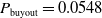 ${P_{\text{buyout}}} = 0.0548$
meaning that the fair buyout premium is 5.48% of the initial liability value L(0). Note that this premium is on top of the assets with value A(0) which we assume to have the same value as the liabilities, that is,
${P_{\text{buyout}}} = 0.0548$
meaning that the fair buyout premium is 5.48% of the initial liability value L(0). Note that this premium is on top of the assets with value A(0) which we assume to have the same value as the liabilities, that is,
 $A(0) = L(0)$
. The additional 5.48% are required to compensate the buyout insurer for covering the risk of deficits occurring in the future. We find that this premium increases significantly from 5.48% to 56.82% when a more risky asset portfolio strategy, that is
$A(0) = L(0)$
. The additional 5.48% are required to compensate the buyout insurer for covering the risk of deficits occurring in the future. We find that this premium increases significantly from 5.48% to 56.82% when a more risky asset portfolio strategy, that is
 $\sigma_A=30\%$
, is applied. The same effect can be observed in a high interest rate environment. In addition, we find that for low volatility investment strategies, that is
$\sigma_A=30\%$
, is applied. The same effect can be observed in a high interest rate environment. In addition, we find that for low volatility investment strategies, that is
 $\sigma_A=2\%$
, the buyout premium increases as a result of a higher mean short rate, but this is the opposite for a high volatility asset strategy.
$\sigma_A=2\%$
, the buyout premium increases as a result of a higher mean short rate, but this is the opposite for a high volatility asset strategy.
The final column in Table 6 shows the product
 $L(0) {P_{\text{buyout}}}$
, that is, the fair buyout premium for a life annuity of 1 per annum. We observe in Table 6 that those premiums are lower in the high interest rate environment. The lowest premium per unit of annual annuity is about 0.71 units in the high interest rate – low volatility environment, and the highest premium is paid in the low interest rate – high volatility setting.
$L(0) {P_{\text{buyout}}}$
, that is, the fair buyout premium for a life annuity of 1 per annum. We observe in Table 6 that those premiums are lower in the high interest rate environment. The lowest premium per unit of annual annuity is about 0.71 units in the high interest rate – low volatility environment, and the highest premium is paid in the low interest rate – high volatility setting.
The dependence of the buyout price
 ${P_{\text{buyout}}}$
on the riskiness of the asset strategy as measured by the volatility
${P_{\text{buyout}}}$
on the riskiness of the asset strategy as measured by the volatility
 $\sigma_A$
is clearly important. We will investigate the role of
$\sigma_A$
is clearly important. We will investigate the role of
 $\sigma_A$
further in Section 5.3.
$\sigma_A$
further in Section 5.3.
In the next step of our simulation study, we add jumps to the mortality rates as specified in (2.3) with
 $v_\mu = 100$
. We consider three possible values for the jump intensity
$v_\mu = 100$
. We consider three possible values for the jump intensity
 $\lambda$
, which we consider to be empirically relevant as they correspond to one, seven or ten mortality shock on average per 100 years,
$\lambda$
, which we consider to be empirically relevant as they correspond to one, seven or ten mortality shock on average per 100 years,
 $\lambda = 0.01, 0.07, 0.1$
. This choice seems justified given the observations in Table 5. The annuity values and buyout premiums calculated from such models are shown in Table 7. Comparing this table to Table 6, we find that the mortality shocks have significant impact on buyout prices for
$\lambda = 0.01, 0.07, 0.1$
. This choice seems justified given the observations in Table 5. The annuity values and buyout premiums calculated from such models are shown in Table 7. Comparing this table to Table 6, we find that the mortality shocks have significant impact on buyout prices for
 $v_{\mu}=100$
. For a lower value of
$v_{\mu}=100$
. For a lower value of
 $v_{\mu}$
, for example 1, only a very small impact is observed for different values of
$v_{\mu}$
, for example 1, only a very small impact is observed for different values of
 $\lambda$
, which can be considered negligible for any practical purposes (Appendix B). This results seems to be particularly relevant in light of the COVID-19 pandemic and the question of how insurers should recalibrate their mortality models. Given our results, we argue that buyout prices are highly sensitive to uncertainty driven by the severity of the pandemic, which can be associated with
$\lambda$
, which can be considered negligible for any practical purposes (Appendix B). This results seems to be particularly relevant in light of the COVID-19 pandemic and the question of how insurers should recalibrate their mortality models. Given our results, we argue that buyout prices are highly sensitive to uncertainty driven by the severity of the pandemic, which can be associated with
 $v_{\mu}$
.
$v_{\mu}$
.
Table 7. Annuity values and buyout prices (and 95% central intervals of the Monte Carlo distribution), with jumps in the mortality rate but no jumps in the short rate or asset price process. The scaling parameters for J in equations (2.3), (2.10) and (2.13) are
 $v_r=0$
,
$v_r=0$
,
 $v_{\mu}=100$
,
$v_{\mu}=100$
,
 $v_A=0$
.
$v_A=0$
.

We now turn to financial shocks, in particular, negative shocks, to the short rate. We first consider such shocks in isolation before looking at shocks affecting both, mortality and interest rates. As we are only allowing downward jumps in interest rates, the inclusion of such jumps reduces the average short rate over the remaining time the pension fund operates. It is therefore no surprise that annuity values increase slightly from Tables 6–8. However, the changes to buyout prices from Tables 6–8 are rather small.
Table 8. Annuity values and buyout prices (and 95% central intervals of the Monte Carlo distribution), with jumps in the short rate but no jumps in the mortality rate or asset price process. The scaling parameters for J in Equations (2.3), (2.10) and (2.13) are
 $v_r=0.02, 0.10$
,
$v_r=0.02, 0.10$
,
 $v_{\mu}=0$
,
$v_{\mu}=0$
,
 $v_A=0$
.
$v_A=0$
.

We now add shocks to mortality and interest rates, referring Model 1, where the shocks affect both dynamics simultaneously. The results for this modelling approach are reported in Table 9, and we find that the buyout prices are significantly different than those reported in Table 6. However, they are only marginally different from those presented in Table 7. Given that introducing a jump process into our short rate model has led to small changes, comparing prices in Tables 6 and 8, it is to be expected that prices obtained in Table 9 are comparable to those in Table 7.
Table 9. Annuity values and buyout prices (and 95% central intervals of the Monte Carlo distribution) in Model 1. The scaling parameters for J in equations (2.3), (2.10) and (2.13) are
 $v_r=0.02, 0.10$
,
$v_r=0.02, 0.10$
,
 $v_{\mu}=100$
,
$v_{\mu}=100$
,
 $v_A=0$
.
$v_A=0$
.

To see the impact of simultaneous shocks as compared to independent shocks, we consider independent shocks affecting mortality and short rates, that is, we have independent jump process
 $J_r$
. The findings are tabulated in Table 10, and, for the low interest rate environment, the results mostly suggest very slight or marginal differences to those presented in Table 9. However, this conclusion changes slightly when a high interest rate environment is considered. Simultaneous jumps can lead to both, higher or lower buyout premiums as compared to independent jumps. Differences are not huge, but in many cases significant in the sense that the 95% intervals are not overlapping.
$J_r$
. The findings are tabulated in Table 10, and, for the low interest rate environment, the results mostly suggest very slight or marginal differences to those presented in Table 9. However, this conclusion changes slightly when a high interest rate environment is considered. Simultaneous jumps can lead to both, higher or lower buyout premiums as compared to independent jumps. Differences are not huge, but in many cases significant in the sense that the 95% intervals are not overlapping.


5.2 Shocks in mortality and asset returns
We add shocks to mortality rates and asset returns as specified in (2.3) and (2.13), respectively, in Model 2. The short rates follow the CIR model, described in (2.7), in this setting. We find that buyout prices, shown in Table 11, in the low interest environment, are slightly higher than the ones obtained in Model 1 in Table 9. However, there is an adverse relationship in the high interest rate environment. There are some significant changes in the high interest rate – low volatility setting when
 $\lambda=0.01$
. For instance, the buyout price for
$\lambda=0.01$
. For instance, the buyout price for
 $v_r=0.1$
in this setting, Table 11, is 11.41% of the initial liability in comparison to 13.09% in Model 1 in Table 9.
$v_r=0.1$
in this setting, Table 11, is 11.41% of the initial liability in comparison to 13.09% in Model 1 in Table 9.
Table 11. Annuity values and buyout prices (and 95% central intervals of the Monte Carlo distribution) in Model 2. The scaling parameters for J in equations (2.3), (2.10) and (2.13) are
 $v_r=0$
,
$v_r=0$
,
 $v_{\mu}=100$
,
$v_{\mu}=100$
,
 $v_A=0.02, 0.10$
.
$v_A=0.02, 0.10$
.

We also calculate buyout prices by replacing the joint jump process J in Model 2 with independent jump process
 $J_A$
for the asset prices. The results are presented in Table 12, indicating almost identical or slightly higher buyout prices to those reported in Table 11.
$J_A$
for the asset prices. The results are presented in Table 12, indicating almost identical or slightly higher buyout prices to those reported in Table 11.


5.3 Asset volatility
We have seen that the asset volatility
 $\sigma_A$
is an important parameter with great impact on the buyout price
$\sigma_A$
is an important parameter with great impact on the buyout price
 ${P_{\text{buyout}}}$
. In addition, the asset volatility can be controlled by the fund managers who decide about the asset mix in the underlying investment with price process A. To have a more complete picture of the role that
${P_{\text{buyout}}}$
. In addition, the asset volatility can be controlled by the fund managers who decide about the asset mix in the underlying investment with price process A. To have a more complete picture of the role that
 $\sigma_A$
plays for pricing buyout contracts, we plot Figures 5–6 showing buyout prices as a function of
$\sigma_A$
plays for pricing buyout contracts, we plot Figures 5–6 showing buyout prices as a function of
 $\sigma_A$
.
$\sigma_A$
.

Figure 5. Buyout prices in Model 1, with and without independent jumps, and the baseline model in addition to shocks affecting mortality or short rate dynamics separately in the low,
 $\theta=0.02$
(left), and high,
$\theta=0.02$
(left), and high,
 $\theta=0.08$
(right), interest rate environments for
$\theta=0.08$
(right), interest rate environments for
 $\lambda=0, 0.1$
;
$\lambda=0, 0.1$
;
 $v_r=0, 0.1$
;
$v_r=0, 0.1$
;
 $v_{\mu}=0,100$
;
$v_{\mu}=0,100$
;
 $v_A=0, 0.1$
.
$v_A=0, 0.1$
.

Figure 6. Buyout prices in Models 1–2, with and without independent jumps, and the baseline model in the low,
 $\theta=0.02$
(left), and high,
$\theta=0.02$
(left), and high,
 $\theta=0.08$
(right), interest rate environments for
$\theta=0.08$
(right), interest rate environments for
 $\lambda=0, 0.1$
;
$\lambda=0, 0.1$
;
 $v_r=0, 0.1$
;
$v_r=0, 0.1$
;
 $v_{\mu}=0,100$
;
$v_{\mu}=0,100$
;
 $v_A=0, 0.1$
.
$v_A=0, 0.1$
.
Figure 5 demonstrates buyout prices in Model 1, with and without independent jumps, along with the baseline model (no jumps) and the models with jumps in the short rates or mortality rates across different asset volatilities between 0.02 and 0.30. The figure shows an increasing trend in buyout prices with respect to an increasing level of asset volatility in both interest rate environments, with a steeper increase for higher values of
 $\sigma_A$
, associated with more risky asset strategies, in the low interest environment
$\sigma_A$
, associated with more risky asset strategies, in the low interest environment
 $\theta=2\%$
. The lowest premiums happen in the no jumps setting for a given asset volatility, followed by the ones with jumps in the short rates. The highest premiums realise in Model 1 with independent jumps, although the rest has remained comparable to those.
$\theta=2\%$
. The lowest premiums happen in the no jumps setting for a given asset volatility, followed by the ones with jumps in the short rates. The highest premiums realise in Model 1 with independent jumps, although the rest has remained comparable to those.
Figure 6 shows buyout premiums across Models 1–2, with and without independent jumps, along with the baseline model (no jumps) in two interest rate environments. Once again the lowest premiums are realised in the baseline model. Although buyout prices look very similar across different models, they are slightly higher in the low interest rate environment for the models with independent jumps, where the differences are bigger in the high interest environment.
6. Discussion and conclusion
We have examined pension buyout prices for a hypothetical population by considering an unexpected upward shock in mortality rates and a simultaneous movement in financial markets. The sensitivity of the buyout price to different parameter values is explored with particular emphasis on contrasting simultaneous shocks to independent shocks.
We observe that there is a significant difference between buyout prices assuming no jumps and prices calculated under the assumption of possible jumps. However, it turns out that the independence assumption is less critical. In fact, we observe only relatively small differences between buyout prices (or annuity values) calculated based on the assumption of independent shocks and simultaneous shocks. In other words as long as the jump intensities are similar, models with independent jump processes lead to similar buyout prices as models with simultaneous jumps. We further see that the changes in buyout prices in the existence of dependence between mortality and short rates are mainly driven by the uncertainty in mortality rates.
On the financial side, asset volatility is the most important factor for buyout prices. Of course, this raises a number of questions since the riskiness of investments can be controlled by fund managers. While it is beyond the scope of this paper, we think that the issue of choosing an appropriate volatility assumption is more important for buyout prices than any of the other parameters in our model. Finally, although life annuity prices decline when mortality increases, we find in Tables 11 and 12 that the impact on related buyout prices depends on the volatility of the assets. For a risky investment strategy with high volatility, we find that buyout processes are lower for higher jump intensities (and lower annuity values). The picture is different for low volatility investment strategies with high jump intensities increasing buyout premiums.
The proposed model has been chosen to be as simple as possible while allowing for common and independent jumps. One possible extension of the model might be to keep common jump times but allow for independent (or weakly dependent) jump sizes. A further possible extension would be replacing the Brownian motion in the LC model with some other process. In discrete time, it is well documented that a random walk is not the best fitting time series model for the period effect.
Another crucial assumption that could be relaxed is that shocks appear simultaneously, that is, markets react immediately to extreme mortality events. This assumption can of course be questioned, in particular, when a pandemic is considered in which excess deaths are observed over a long time horizon. As mentioned in the introduction, we consider our approach a good approximation given the long-term nature of the considered buyout contract. A detailed modelling of the delay with which markets react to mortality events would be a very useful extension and could be built into our proposed methodology. However, this would require a very carefully tuned model to avoid arbitrage opportunities that might arise if market reactions are predictable.
Another line of research could further extend our model and our numerical analysis by considering further risk factors in the financial market that might have an impact on pension fund portfolios, for example exchange rates, inflation. In this context, it would also be interesting to consider models where a mortality shock has an impact on several financial risk factors. In our numerical study, we focused on one risk factor only (either interest rates or asset prices) to identify the effect that a shock in each of those has on buyout prices. However, this assumption could be relaxed by considering a simulation set-up in which a mortality shock impacts several risk factors simultaneously. Yet again, this might require a carefully tuned model to avoid potential inter-correlations across different dynamics while pricing pension buyouts.
To gain further insight into the question of how important the independence assumption is, one could fine-tune the simulation study by choosing a wider range of possible parameters or, even better, choose parameters based on an empirical study that aims to fit a joint model to mortality, interest rates and share prices. However, we would expect that the rarity of large mortality shocks, see table Table 5, and the general volatility in the financial market would make the resulting estimates rather unreliable with very wide confidence intervals.
Acknowledgements
This study was part of the research programme at the Research Centre for Longevity Risk – a joint initiative of NN Group and the University of Amsterdam, with additional funding from the Dutch government’s Public Private Partnership programme.
Conflicts of interest
The author(s) declare none.
Appendix A. Interpolation method
Let us assume that we would like to calculate a life annuity value for a pair of
 $(\mu, r)$
, where
$(\mu, r)$
, where
 $\mu^{i} < \mu < \mu^{i+1}$
and
$\mu^{i} < \mu < \mu^{i+1}$
and
 $r^{j} < r < r^{j+1}$
, using one of the preprocessed tables, for example Table 2. Also, for now, suppose that the relevant life annuity value, a(t, x), is represented by
$r^{j} < r < r^{j+1}$
, using one of the preprocessed tables, for example Table 2. Also, for now, suppose that the relevant life annuity value, a(t, x), is represented by
 $a_{t}(\mu, r)$
as a function of
$a_{t}(\mu, r)$
as a function of
 $\mu$
and r. Following Feng et al. (Reference Feng, Cui and Li2016), the corresponding life annuity value can be obtained as
$\mu$
and r. Following Feng et al. (Reference Feng, Cui and Li2016), the corresponding life annuity value can be obtained as
 \begin{eqnarray*} a_{t}\big(\mu, r^j \big) &=& \frac{\mu^{i+1} - \mu }{\mu^{i+1} - \mu^{i} }\, a_{t} \big(\mu^{i}, r^{j}\big) + \frac{\mu - \mu^i }{\mu^{i+1} - \mu^{i} }\, a_{t} \big(\mu^{i+1}, r^{j}\big)\\[5pt] a_{t}\big(\mu, r^{j+1} \big) &=& \frac{\mu^{i+1} - \mu }{\mu^{i+1} - \mu^{i} }\, a_{t} \big(\mu^{i}, r^{j+1}\big) + \frac{\mu - \mu^i }{\mu^{i+1} - \mu^{i} }\, a_{t} \big(\mu^{i+1}, r^{j+1}\big)\\[5pt] a_{t}\big(\mu, r \big) &=& \frac{r^{j+1} - r }{r^{j+1} - r^{j} }\, a_{t} \big(\mu, r^{j}\big) + \frac{r - r^j }{r^{j+1} - r^{j} } \, a_{t} \big(\mu, r^{j+1}\big). \end{eqnarray*}
Appendix B. Annuity values and buyout prices in high interest rate scenario


Appendix C. Buyout prices for different values of
 $v_{\mu}$
and
$v_r$
in high and low interest rate scenarios
$v_{\mu}$
and
$v_r$
in high and low interest rate scenarios


Table C.1. Buy-out prices (and 95% central intervals of the Monte Carlo distribution) in Model 1. The scaling parameters for J in equations (2.3), (2.10) and (2.13) are
 $v_r=0.5, \,5, \,50, \,80$
,
$v_r=0.5, \,5, \,50, \,80$
,
 $v_{\mu}=0.5, \,5, \,50, \,80$
,
$v_{\mu}=0.5, \,5, \,50, \,80$
,
 $v_A=0$
,
$v_A=0$
,
 $\lambda = 0.1$
.
$\lambda = 0.1$
.


Figure C.1. Buyout prices in Model 1 for selected values of
 $v_{\mu}$
for
$v_{\mu}$
for
 $v_r=0.5$
(left) and
$v_r=0.5$
(left) and
 $v_r=80$
(right) in the low,
$v_r=80$
(right) in the low,
 $\theta=0.02$
, and high,
$\theta=0.02$
, and high,
 $\theta=0.08$
, interest rate environments for
$\theta=0.08$
, interest rate environments for
 $\lambda=0.1$
;
$\lambda=0.1$
;
 $v_{\mu}=0.5, 80$
;
$v_{\mu}=0.5, 80$
;
 $v_A=0$
.
$v_A=0$
.
Appendix D. Contour plots for life annuity premiums in low interest rate scenarios

Figure D.1. Contour plots for life annuity contracts when
 $\lambda=0.1$
,
$\lambda=0.1$
,
 $v_r=0.1$
,
$v_r=0.1$
,
 $v_{\mu} = 0$
and
$v_{\mu} = 0$
and
 $\theta=0.08$
.
$\theta=0.08$
.

Figure D.2. Contour plots for life annuity contracts when
 $\lambda=0.1$
,
$\lambda=0.1$
,
 $v_r=0$
,
$v_r=0$
,
 $v_{\mu} = 100$
and
$v_{\mu} = 100$
and
 $\theta=0.08$
.
$\theta=0.08$
.

Figure D.3. Contour plots for life annuity contracts when
 $\lambda=0.1$
,
$\lambda=0.1$
,
 $v_r=0.1$
,
$v_r=0.1$
,
 $v_{\mu} = 100$
and
$v_{\mu} = 100$
and
 $\theta=0.08$
.
$\theta=0.08$
.
Appendix E. Contour plots for life annuity premiums in low interest rate scenarios

Figure E.1. Contour plots for life annuity contracts based on Model 0 when
 $\theta$
is 0.02.
$\theta$
is 0.02.

Figure E.2. Contour plots for life annuity contracts when
 $\lambda=0.1$
,
$\lambda=0.1$
,
 $v_r=0.1$
,
$v_r=0.1$
,
 $v_{\mu} = 0$
and
$v_{\mu} = 0$
and
 $\theta=0.02$
.
$\theta=0.02$
.

Figure E.3. Contour plots for life annuity contracts when
 $\lambda=0.1$
,
$\lambda=0.1$
,
 $v_r=0$
,
$v_r=0$
,
 $v_{\mu} = 100$
and
$v_{\mu} = 100$
and
 $\theta=0.02$
.
$\theta=0.02$
.

Figure E.4. Contour plots for life annuity contracts when
 $\lambda=0.1$
,
$\lambda=0.1$
,
 $v_r=0.1$
,
$v_r=0.1$
,
 $v_{\mu} = 100$
and
$v_{\mu} = 100$
and
 $\theta=0.02$
.
$\theta=0.02$
.

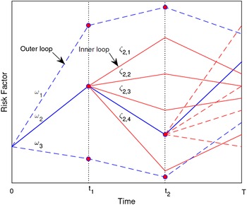


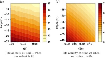

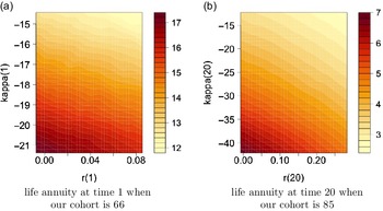


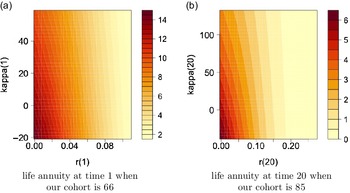


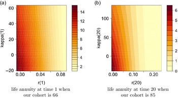


 Open access