

1. Introduction
Due to the longevity phenomenon, forecasting mortality has become more and more important for actuaries, pension sponsors and policymakers. Since the seminal work of Lee and Carter (Reference Lee and Carter1992), (dynamic) factor models (DFMs), including the Lee–Carter (LC), the Cairns–Blake–Dowd (CBD) models (Cairns et al., Reference Cairns, Blake and Dowd2006) and others (see e.g., French and O’Hare, Reference French and O’Hare2013; Chulia et al., Reference Chulia, Guillen and Uribe2016; Heinemann, 2017; Gao et al., Reference Gao, Shang and Yang2019; He et al., Reference He, Huang, Shi and Yang2021), have become the workhorse for mortality modelling.Footnote 1 Their mathematical simplicity can partly explain this success story since they assume that a small number of factor processes drive age-specific mortality rates. For instance, in the LC model, the log-mortality rates $\log m_{x,t}$
at time t are driven by the same factor across different ages. However, depending on the data at hand, this simple factor structure might be too restrictive to describe the evolution of the mortality dynamics adequately. In particular, empirical studies often find that the inclusion of a cohort effect, that is a process indexed by
$\log m_{x,t}$
at time t are driven by the same factor across different ages. However, depending on the data at hand, this simple factor structure might be too restrictive to describe the evolution of the mortality dynamics adequately. In particular, empirical studies often find that the inclusion of a cohort effect, that is a process indexed by $t-x$
, improves the fit of the model significantly, but the identification and estimation of such age-period-cohort models is often difficult (see e.g., Kuang et al., Reference Kuang, Nielsen and Nielsen2008; Hunt and Villegas, Reference Hunt and Villegas2015).
$t-x$
, improves the fit of the model significantly, but the identification and estimation of such age-period-cohort models is often difficult (see e.g., Kuang et al., Reference Kuang, Nielsen and Nielsen2008; Hunt and Villegas, Reference Hunt and Villegas2015).
The downside of such DFMs is also well documented in the time series literature. As Lin and Michailidis (Reference Lin and Michailidis2020) put it, “the identification of factors is often problematic, especially when we wish to give them an economic interpretation…. even when all such ‘common’ factors are taken into account, there will be important residual interdependencies … that remain to be explained”. One popular alternative that has emerged in the past several decades is the Vector Autoregressive (VAR) model. These models do not assume a factor structure and are thus much more flexible than DFMs. The mortality modelling community has recently also started to embrace VAR models as a strong competitor to factor models (Lazar and Denuit, Reference Lazar and Denuit2009). Nevertheless, the application of VAR models to high-dimensional time series is not straightforward due to the curse of dimensionality. In particular, while in typical, economic applications, the dimension of the time series is often less than 10, and this number can easily reach 100 or larger in the context of mortality modelling, leading to a huge number of parameters (5000) even in the simplest, first-order [VAR(1)] case. Moreover, mortality data are usually only available annually, with $T<100$
. This has forced existing VAR-type mortality papers to introduce parametric constraints. These constraints can be either a priori given or data-driven. For instance, Li and Lu (Reference Li and Lu2017) assume that the only non-zero elements of the coefficient matrix are on the diagonal (corresponding to the regression coefficients of their own lags), or the second (respectively the third) lower diagonal (corresponding to the regression coefficients of their adjacent lags). Although the model of Li and Lu (Reference Li and Lu2017) has the appealing property of ensuring co-integration of the log-mortality rates for any pair of ages, their sparsity constraint on the coefficient matrix is quite restrictive and has been questioned by the subsequent literature (see, e.g., Doukhan et al., Reference Doukhan, Pommeret, Rynkiewicz and Salhi2017; Guibert et al., Reference Guibert, Lopez and Piette2019; Shi, Reference Shi2020; Feng et al., Reference Feng, Shi and Chang2021; Chang and Shi, Reference Chang and Shi2021). Alternative regularisation methods, such as the elastic net and the Lasso, have been proposed to address the curse of dimensionality. These recent contributions, though, also have their limitations.
$T<100$
. This has forced existing VAR-type mortality papers to introduce parametric constraints. These constraints can be either a priori given or data-driven. For instance, Li and Lu (Reference Li and Lu2017) assume that the only non-zero elements of the coefficient matrix are on the diagonal (corresponding to the regression coefficients of their own lags), or the second (respectively the third) lower diagonal (corresponding to the regression coefficients of their adjacent lags). Although the model of Li and Lu (Reference Li and Lu2017) has the appealing property of ensuring co-integration of the log-mortality rates for any pair of ages, their sparsity constraint on the coefficient matrix is quite restrictive and has been questioned by the subsequent literature (see, e.g., Doukhan et al., Reference Doukhan, Pommeret, Rynkiewicz and Salhi2017; Guibert et al., Reference Guibert, Lopez and Piette2019; Shi, Reference Shi2020; Feng et al., Reference Feng, Shi and Chang2021; Chang and Shi, Reference Chang and Shi2021). Alternative regularisation methods, such as the elastic net and the Lasso, have been proposed to address the curse of dimensionality. These recent contributions, though, also have their limitations.
First, unlike Li and Lu (Reference Li and Lu2017) and the original LC and CBD models, these latter models are not written on the level of the log-mortality,Footnote 2 but on their first-order difference, that is the mortality improvement rate. Even though the dilemma of whether to differentiate the series before applying VAR-type models arises frequently both in the economic (see, e.g., Williams, Reference Williams1978) and actuarial literature (Haberman and Renshaw, Reference Haberman and Renshaw2012; Mitchell et al., Reference Mitchell, Brockett, Mendoza-Arriaga and Muthuraman2013; Chulia et al., Reference Chulia, Guillen and Uribe2016; Guibert et al., Reference Guibert, Lopez and Piette2019; Jarner and Jallbjørn, 2020), we believe that the differentiation approach has several downsides. Indeed, models written on the differences (implicitly) assume that mortality rates are first-order integrated (i.e., I(1)). This assumption is usually made out of mathematical convenience, without being tested against other alternative hypothesis. Moreover, while the theory on unit root tests of univariate time series is well documented, their performance in a small-T context is known to be often unsatisfactory. Moreover, when applied to the $(\kappa_{t})$
process estimated from the LC model, the result of the tests should be interpreted very carefully, since
$(\kappa_{t})$
process estimated from the LC model, the result of the tests should be interpreted very carefully, since $\kappa_{t}$
is not directly observed, but can only be indirectly estimated and is hence subject to estimation error. For instance, the unit root hypothesis in the LC model has recently been questioned by Leng and Peng (Reference Leng and Peng2016). Furthermore, even if the I(1) assumption holds true, a model written on the improvement rates is not able to detect potential co-integration relationships. In some cases, such properties might be desirable, since they spell biological reasonableness, that is, the mortality at different ages do not diverge. Interestingly, this assumption is not imposed in the original, LC model, but was merely an empirically plausible specification, when the model was applied to the US data.
$\kappa_{t}$
is not directly observed, but can only be indirectly estimated and is hence subject to estimation error. For instance, the unit root hypothesis in the LC model has recently been questioned by Leng and Peng (Reference Leng and Peng2016). Furthermore, even if the I(1) assumption holds true, a model written on the improvement rates is not able to detect potential co-integration relationships. In some cases, such properties might be desirable, since they spell biological reasonableness, that is, the mortality at different ages do not diverge. Interestingly, this assumption is not imposed in the original, LC model, but was merely an empirically plausible specification, when the model was applied to the US data.
Second, Guibert et al. (Reference Guibert, Lopez and Piette2019) report that when fitting large VAR(p) models on mortality improvement rates, a large p typically leads to better fit. This may be an indication of likely over-differentiation. This issue also raises further concerns about the curse of dimensionality (especially in a small T context), as well as the choice of the optimal order. Guibert et al. (Reference Guibert, Lopez and Piette2019) propose to fix a prior p, and they acknowledge that “by increasing the lag order (and by using regularisation techniques), some non-null coefficients can be forced to zero in favour of other coefficients in autoregressive matrices of higher lag order.”
A potential alternative to VAR(p) models is the Vector Autoregressive and Moving Average (VARMA) models. The VARMA model is, roughly speaking, the multivariate analogue of ARMA process and is hence a legitimate, parsimonious competitor of VAR(p). However, their application to time series data is still in its infancy due to (i) identification difficulties that are proper to (multivariate) VARMA models (see e.g., Gouriéroux et al., Reference Gouriéroux, Monfort and Renne2020); (ii) the much more complicated, non-linear estimation procedure (see e.g., Litterman, Reference Litterman1986; Chan and Eisenstat, Reference Chan and Eisenstat2017), compared to the Ordinary Least Square (OLS)-type estimators frequently employed for VAR models.
This paper proposes to solve the aforementioned challenges through a new approach, called Factor-Augmented VAR (or FAVAR) model. This model, first introduced by Bernanke et al. (Reference Bernanke, Boivin and Eliasz2005), is a trade-off between standalone DFM and VAR models and has since received much attention in (macro-) econometrics (see e.g., Dufour and Stevanović, Reference Dufour and Stevanović2013; Bai et al., Reference Bai, Li and Lu2016). The original FAVAR formulation has also evolved and given rise to several variants depending on the specific application. In particular, recently, Chan and Eisenstat (Reference Chan and Eisenstat2015) propose a new specification, which, roughly speaking, is obtained from the VAR(1) model by adding one unobserved factor process. This factor allows for a natural, systemic (longevity) risk factor interpretation, similar to the $(\kappa_{t})$
process in the LC model. This feature is especially instructive and interesting since this way, the model allows for DFM and VAR models as special cases, and hence naturally enjoys many of the better properties of both elementary models that are well known to actuaries. On the one hand, the FAVAR model inherits VAR’s flexibility of capturing serial correlation. On the other hand, the common factor extends the VAR(1) model, while at the same time being much more parsimonious than the aforementioned alternative extensions such as VAR(p) and VARMA models. Finally, by gathering the LC and the VAR approach within the same framework, the FAVAR model also makes model comparison much more convenient.
$(\kappa_{t})$
process in the LC model. This feature is especially instructive and interesting since this way, the model allows for DFM and VAR models as special cases, and hence naturally enjoys many of the better properties of both elementary models that are well known to actuaries. On the one hand, the FAVAR model inherits VAR’s flexibility of capturing serial correlation. On the other hand, the common factor extends the VAR(1) model, while at the same time being much more parsimonious than the aforementioned alternative extensions such as VAR(p) and VARMA models. Finally, by gathering the LC and the VAR approach within the same framework, the FAVAR model also makes model comparison much more convenient.
We propose to estimate the FAVAR model in a Bayesian fashion, using the state-of-the-art shrinkage prior (or Minnesota prior) developed in the Bayesian VAR (BVAR) literature. This approach, introduced by Litterman (Reference Litterman1986), is instrumental in dealing with the curse of dimensionality through Bayesian shrinkage. More precisely, the prior distribution has the effect of “pushing” the posterior distribution towards some benchmark model. This latter will be chosen by the user of our model, according to his/her prior belief, as well as other constraints he/she wants to put in place, such as biological reasonableness, which rules out long-term divergence of logged mortality rates at different ages. For instance, in the empirical section, we let the prior distribution of the parameters to be concentrated around a value corresponding to the sparse VAR proposed in Li and Lu (Reference Li and Lu2017). Our choice of the prior can be viewed as the Bayesian analogue of the frequentist regularization techniques already known to the mortality literature. This interpretation is particularly interesting, given the Bayesian posterior median interpretation of the Lasso estimate in a linear regression setting (see Tibshirani, Reference Tibshirani1996; Park and Casella, Reference Park and Casella2008). Note that recently, Bayesian Lasso (Billio et al., Reference Billio, Casarin and Rossini2019) and elastic net models (Gefang, Reference Gefang2014) have also gained popularity and are thus a possible alternative to the Minnesota prior. Nevertheless, in light of the recent debate on sparsity versus density (Giannone et al., Reference Giannone, Lenza and Primiceri2021), we opt for the Minnesota-type shrinkage prior over Lasso-type methods.
Compared to the existing frequentist regularisation approaches in the mortality literature, our Bayesian approach has several distinctive advantages. First, it naturally introduces parameter uncertainty, which is essential for stress testing and risk management in the pension and insurance industries. In particular, because pension and annuity products are typically indexed to macroeconomic and financial indicators, both need to be forecast or simulated by the financial economist/pension sponsor. Consequently, a unified modelling framework would be highly welcome. BVAR-type models are natural candidates given their strong popularity in macroeconomic forecasting, especially when quantifying forecasting uncertainty. Second, because the FAVAR model (as well as the LC and CBD models) involves an unobserved factor, it belongs to the family of state-space models. In the actuarial literature, such models are typically estimated using a two-step approach. First, the latent factor(s) path is estimated from the raw mortality time series, as if they were deterministically given. These estimated paths are then used in the second stage to estimate the dynamics of the factor process. This approach induces efficiency loss (see Bernanke et al., Reference Bernanke, Boivin and Eliasz2005 for a discussion), and to make things worse, Leng and Peng (Reference Leng and Peng2016) show that they are asymptotically inconsistent, even in the plain LC model. A more rigorous, but cumbersome way is to compute the likelihood function in one step by integrating out all possible paths of the latent factor. This can be done both frequentistly and in a Bayesian way. Under the frequentist approach, the model parameter is first estimated, then the path of the latent factor is filtered out. If the modeller were to further measure parameter uncertainty, the filtering exercise needs to be conducted for each draw of the parameter value, making the computation formidable. The strength of the Bayesian approach here is it combines the parameter estimation and factor filtering tasks in one step. This is the approach we take, and we rely on state-of-the-art Markov chain Monte Carlo (MCMC) techniques to minimise the computational burden.
Despite these benefits, the use of Bayesian methods in mortality modelling is still sparse and has been largely confined to DFM models (Czado et al., Reference Czado, Delwarde and Denuit2005; Pedroza, Reference Pedroza2006; Reichmuth and Sarferaz, Reference Reichmuth and Sarferaz2008; Cairns et al., Reference Cairns, Blake, Dowd, Coughlan and Khalaf-Allah2011; Antonio et al., Reference Antonio, Bardoutsos and Ouburg2015; Li et al., Reference Li, De Waegenaere and Melenberg2015; van Berkum et al., Reference van Berkum, Antonio and Vellekoop2017; Alexopoulos et al., Reference Alexopoulos, Dellaportas and Forster2019; Li et al., Reference Li, Zhou, Zhu, Chan and Chan2019; Wang et al., Reference Wang, Pantelous and Vahid2021).Footnote 3 To our knowledge, the only paper employing BVAR to mortality data is Njenga and Sherris (Reference Njenga and Sherris2020). These authors first fit the three-parameter Heligman–Pollard model to the age-specific, cross-sectional mortality tables for each year t to obtain a three-dimensional process of parameters $\theta_{t}$
, which they then use to fit the BVAR model. Besides the fact that our FAVAR model includes an extra latent factor, our approach further differs from theirs in several aspects. First, Njenga and Sherris (Reference Njenga and Sherris2020) adopt the “sum of coefficient” prior (Sims and Zha, Reference Sims and Zha1998). This latter, which is also an extension of the Minnesota prior, assumes a priori the existence of (co)-integration. Even though we could also follow this route, in this paper, we take a different approach and construct our prior by inspiring directly from the original Minnesota prior, without imposing non-stationarity (see our discussions above). Second, similar to the LC model, it is unclear how the estimation error induced during the fitting of the Heligman–Pollard model impacts the estimation at the second BVAR stage. Thirdly, the BVAR model fitted to
$\theta_{t}$
, which they then use to fit the BVAR model. Besides the fact that our FAVAR model includes an extra latent factor, our approach further differs from theirs in several aspects. First, Njenga and Sherris (Reference Njenga and Sherris2020) adopt the “sum of coefficient” prior (Sims and Zha, Reference Sims and Zha1998). This latter, which is also an extension of the Minnesota prior, assumes a priori the existence of (co)-integration. Even though we could also follow this route, in this paper, we take a different approach and construct our prior by inspiring directly from the original Minnesota prior, without imposing non-stationarity (see our discussions above). Second, similar to the LC model, it is unclear how the estimation error induced during the fitting of the Heligman–Pollard model impacts the estimation at the second BVAR stage. Thirdly, the BVAR model fitted to $(\theta_{t})$
does not guarantee the positivity of its components, leaving room to potentially implausible scenarios. Fourthly, since the Heligman–Pollard model involves a non-linear transformation from
$(\theta_{t})$
does not guarantee the positivity of its components, leaving room to potentially implausible scenarios. Fourthly, since the Heligman–Pollard model involves a non-linear transformation from $\theta_{t}$
to the vector of age-specific mortality rates, a potential, linear (co)-integration property of process
$\theta_{t}$
to the vector of age-specific mortality rates, a potential, linear (co)-integration property of process $(\theta_{t})$
typically does not translate into linear (co)-integration relationships of the log-mortality rates. In other words, it is difficult to compare this specification with existing approaches, especially when it comes to the resulting, long-run dynamics of the mortality rate process. Fifthly, since parameter
$(\theta_{t})$
typically does not translate into linear (co)-integration relationships of the log-mortality rates. In other words, it is difficult to compare this specification with existing approaches, especially when it comes to the resulting, long-run dynamics of the mortality rate process. Fifthly, since parameter $\theta_{t}$
is low-dimensional, the BVAR’s advantage of parameter shrinkage is less pronounced. Finally, Njenga and Sherris (Reference Njenga and Sherris2020) do not describe the estimation of their model. Given that our model has a large number (around 6000) of parameters and it differs from BVAR by the introduction of an extra factor, we feel it helpful to provide the actuarial community with a step-by-step introduction to the estimation of BVAR and FAVAR models.
$\theta_{t}$
is low-dimensional, the BVAR’s advantage of parameter shrinkage is less pronounced. Finally, Njenga and Sherris (Reference Njenga and Sherris2020) do not describe the estimation of their model. Given that our model has a large number (around 6000) of parameters and it differs from BVAR by the introduction of an extra factor, we feel it helpful to provide the actuarial community with a step-by-step introduction to the estimation of BVAR and FAVAR models.
Our model is illustrated using data from two populations: US males and French males. These two datasets differ in several key aspects. First, the US data have a very small time series dimension ( $T<100$
), whereas observations start as early as 1816 in the French case. This difference of the sample size has implications on the different ability of the Bayesian model to “learn” from the data. In particular, the difference between our estimated FAVAR model and the Li and Lu model is far more important for the French males than for American males. This result demonstrates the necessity of introducing more flexible models, especially when the sample size of a dataset is large enough to warrant such an extension. Second, Li and Lu (Reference Li and Lu2017)’s model works well only on the US data, but much less so on the French ones. In the empirical section, we explain how this preliminary finding can be used to guide the specification of our prior distribution,. Overall, we show that the FAVAR model performs significantly better than the LC and the sparse VAR model.
$T<100$
), whereas observations start as early as 1816 in the French case. This difference of the sample size has implications on the different ability of the Bayesian model to “learn” from the data. In particular, the difference between our estimated FAVAR model and the Li and Lu model is far more important for the French males than for American males. This result demonstrates the necessity of introducing more flexible models, especially when the sample size of a dataset is large enough to warrant such an extension. Second, Li and Lu (Reference Li and Lu2017)’s model works well only on the US data, but much less so on the French ones. In the empirical section, we explain how this preliminary finding can be used to guide the specification of our prior distribution,. Overall, we show that the FAVAR model performs significantly better than the LC and the sparse VAR model.
The paper is organised as follows. Section 2 introduces the FAVAR model. Section 3 describes the Bayesian estimation approach, which is inspired and adapted from the BVAR literature. Section 4 applies the methodology to US and French male mortality data and compares it with the benchmark models of Lee and Carter (Reference Lee and Carter1992) and Li and Lu (Reference Li and Lu2017). Section 5 concludes.
2. The model
2.1. Review of existing mortality models
Let us denote $m_{x,t}$
, the mortality rate at age x and date t, a high-dimensional time series observed over time. The mortality modelling literature has recently focused on two strands of models, namely the dynamic factor model and the VAR-type model.
$m_{x,t}$
, the mortality rate at age x and date t, a high-dimensional time series observed over time. The mortality modelling literature has recently focused on two strands of models, namely the dynamic factor model and the VAR-type model.
The original LC model specifies the log-mortality rates $\log m_{x,t}$
are driven by the same factor across different ages:
$\log m_{x,t}$
are driven by the same factor across different ages:
 \begin{equation*}\log m_{x,t}=a_{x}+b_{x}\kappa_{t}+\epsilon_{x,t},\qquad\forall x,t,\end{equation*}
where $a_{x}$
and
$a_{x}$
and $b_{x}$
are age-specific intercept and slope, respectively, and
$b_{x}$
are age-specific intercept and slope, respectively, and $\epsilon_{x,t}$
is an normally distributed i.i.d error term. To project the processes forward, the standard trick is to consider
$\epsilon_{x,t}$
is an normally distributed i.i.d error term. To project the processes forward, the standard trick is to consider
 \begin{equation*}\kappa_{t}=\gamma+\kappa_{t-1}+\eta_{t},\eta_{t}\sim N(0,\sigma_{\eta}^{2}).\end{equation*}
Several variants of this dynamic factor model, including the two-factor CBD model (Cairns et al., Reference Cairns, Blake and Dowd2006) and others (see, e.g., Heinemann, 2017), have been introduced to the mortality literature.
The VAR(p) model, instead of using a low-dimensional dynamic factors explaining the high-dimensional mortality movements, assumes that
 \begin{equation*}\log m_{x,t}=\alpha_{x,0}+\sum_{i=1}^{p}\sum_{j=0}^{d-1}\alpha_{x,x_{0}+j}^{i}\log(m_{j,t-i})+\epsilon_{x,t}\;\forall x,t,\end{equation*}
where $d$ is the total number of ages for which mortality data are available. The model is highly parameterised that the mortality literature has only considered VAR with one lag case. Even in the one lag case, the number of parameters is $(d+1)d$
, and Li and Lu (Reference Li and Lu2017) specifies the sparse version of it as
$(d+1)d$
, and Li and Lu (Reference Li and Lu2017) specifies the sparse version of it as
 \begin{equation*}\log m_{x,t}=\alpha_{x,0}+\alpha_{x,1}\log m_{x,t-1}+\alpha_{x,2}\log m_{x+1,t-1}+\alpha_{x,3}\log m_{x+2,t-1}+\epsilon_{x,t},\ \forall x,t\end{equation*}
subject to the constraints:
 \begin{align*}\alpha_{x,1}+\alpha_{x,2}+\alpha_{x,3} & =1,\forall x\\[5pt]\alpha_{x,k} & \geq0,\forall x,k=1,2,3.\end{align*}
Li and Lu show that the additional constraints above ensure the co-integration of these processes.
2.2. The FAVAR model
The two base models of the previous section motivated us to consider the following model written on the log-mortality rates:
 \begin{equation}\log(m_{x,t})=a_{x}+\sum_{j=0}^{d-1}a_{x,x_{0}+j}\log(m_{j,t-1})+b_{x}\kappa_{t}+\epsilon_{x,t},\end{equation}
where $x_{0}$
is the lowest age for which mortality rates are observable,
$x_{0}$
is the lowest age for which mortality rates are observable, $(\epsilon_{t})$
is an i.i.d. random vector satisfying:
$(\epsilon_{t})$
is an i.i.d. random vector satisfying:
 \begin{equation}\epsilon_{t}=\left\{ \epsilon_{x_{0},t},....,\epsilon_{x_{0}+d-1,t}\right\} \sim N\left(0,diag\left(S\right)\right),\qquad\textrm{with}\qquad S=(\sigma_{0}^{2},....,\sigma_{d-1}^{2})',\end{equation}
and factor $(\kappa_{t})$
is unobservable, following the dynamics:
$(\kappa_{t})$
is unobservable, following the dynamics:
 \begin{equation}\kappa_{t}=\gamma_{1}+\gamma_{2}\kappa_{t-1}+\eta_{t},\end{equation}
where $(\eta_{t})$
is another i.i.d. sequence and is mutually independent with
$(\eta_{t})$
is another i.i.d. sequence and is mutually independent with $(\epsilon_{t})$
, following:
$(\epsilon_{t})$
, following:
 \begin{equation}\eta_{t}\sim N(0,\sigma_{\eta}^{2}).\end{equation}
Equation (2) implies, among others, that $\epsilon_{x,t},x=1,2,...$
are mutually independent. This assumption, borrowed from the LC model, has recently been relaxed in VAR-type mortality models such as Li and Lu (Reference Li and Lu2017) and Guibert et al. (Reference Guibert, Lopez and Piette2019), using a two-stage approach. The first stage is a Seemingly Unrelated Regression (SUR), that is, the coefficient matrix of the VAR model is estimated as if the different components of
$\epsilon_{x,t},x=1,2,...$
are mutually independent. This assumption, borrowed from the LC model, has recently been relaxed in VAR-type mortality models such as Li and Lu (Reference Li and Lu2017) and Guibert et al. (Reference Guibert, Lopez and Piette2019), using a two-stage approach. The first stage is a Seemingly Unrelated Regression (SUR), that is, the coefficient matrix of the VAR model is estimated as if the different components of $\epsilon_{t}$
are independent. Then the pseudo-residuals are recovered and used to compute the empirical estimator of the covariance matrix. However, in this paper, we will stick with the independence assumption for two reasons. First, this is the assumption retained in Litterman’s Minnesota prior and is also adopted by Njenga and Sherris (Reference Njenga and Sherris2020). Second, restricting the covariance matrix to be diagonal leads to an important dimension reduction and makes the MCMC computation much simpler (see Section 3 for details). Third, since process
$\epsilon_{t}$
are independent. Then the pseudo-residuals are recovered and used to compute the empirical estimator of the covariance matrix. However, in this paper, we will stick with the independence assumption for two reasons. First, this is the assumption retained in Litterman’s Minnesota prior and is also adopted by Njenga and Sherris (Reference Njenga and Sherris2020). Second, restricting the covariance matrix to be diagonal leads to an important dimension reduction and makes the MCMC computation much simpler (see Section 3 for details). Third, since process $(y_{t})$
likely features non-stationarity, the impact of the mis-specification of the covariance matrix could be much smaller than a potential mis-specification of the coefficient matrix. Fourth, it is well known that the (frequentist) estimation of covariance matrix without constraint is highly unreliable in large dimensions (see e.g., Ledoit and Wolf, Reference Ledoit and Wolf2003), and this is especially the case in the SUR framework, given the efficiency loss induced during the first stage. As we will explain in detail in the next section, even though there are standard Bayesian tools to handle the non-diagonal covariance matrix, the curse of dimensionality issue remains acute.
$(y_{t})$
likely features non-stationarity, the impact of the mis-specification of the covariance matrix could be much smaller than a potential mis-specification of the coefficient matrix. Fourth, it is well known that the (frequentist) estimation of covariance matrix without constraint is highly unreliable in large dimensions (see e.g., Ledoit and Wolf, Reference Ledoit and Wolf2003), and this is especially the case in the SUR framework, given the efficiency loss induced during the first stage. As we will explain in detail in the next section, even though there are standard Bayesian tools to handle the non-diagonal covariance matrix, the curse of dimensionality issue remains acute.
Note that in the above model, the factor $\kappa_{t}$
is only identified up to an affine transformation. Thus, for identification purpose, we shall let
$\kappa_{t}$
is only identified up to an affine transformation. Thus, for identification purpose, we shall let
 \begin{equation}b_{x_{0}}=1.\end{equation}
We set the initial $\kappa,\kappa_{0},$
as a model parameter. This identification condition is slightly different from the standard one used in the LC model but is much more common in the literature on factor models and has also been mentioned as an alternative in Section 6 of their paper.
$\kappa,\kappa_{0},$
as a model parameter. This identification condition is slightly different from the standard one used in the LC model but is much more common in the literature on factor models and has also been mentioned as an alternative in Section 6 of their paper.
The proposed approach also shares some similar spirit but is yet different from the so-called Global Vector Autoregressive (GVAR) model. This latter, introduced by Pesaran et al. (Reference Pesaran, Schuermann and Weiner2004) in macro-econometrics to model the dependence of economic variables across different countries, has recently been applied in mortality forecasting by Li and Shi (Reference Li and Shi2021). There are several major differences between our model and the GVAR. First, the GVAR model is mostly appropriate in a multiple-population framework, in which mortality rates of different countries are first modelled separately with a VAR model, and then the different countries are linked together through the GVAR. In the case of single population mortality, it is less natural to separate ex ante the set of all ages into different groups. Our model, on the other hand, is mainly motivated by a single-population framework.Footnote 4 Secondly, although the GVAR specification also adds a factor into a VAR model, this factor is usually assumed observable, such as a linear combination of the observed time series of interest with pre-fixed weights (Li and Shi, Reference Li and Shi2021). Put differently, the GVAR model does not allow for the LC or other factor model as special cases.Footnote 5
Our approach of combining VAR and factor models is also different from the approach of Bernanke et al. (Reference Bernanke, Boivin and Eliasz2005), Biffis and Millossovich (Reference Biffis and Millossovich2006), Debón et al. (Reference Debón, Montes, Mateu, Porcu and Bevilacqua2008), and Mavros et al. (Reference Mavros, Cairns, Streftaris and Kleinow2017). This latter literature propose to first fit a factor model, recover the residuals and then estimate a VAR-type model on these residuals. Even though it would be interesting to compare these two approaches in the future, we note that in these latter models, the status of the DFM and VAR models are different, since the DFM is used as the benchmark, whereas the VAR is merely used as a means to improve the fit of the DFM.
Factor-augmented VAR representation. The above model can be more conveniently represented using a matrix, factor VAR form:
 \begin{align*}y_{t} & =a+Ay_{t-1}+\kappa_{t}b+\epsilon_{t},\end{align*}
where $y_{t}=\left\{ \log(m_{x_{0},t}),...,\log(m_{x_{0}+d-1,t})\right\}^{\prime},a=\left\{ a_{x_{0}},...,a_{x_{0}+d-1}\right\}^{\prime},b=\left\{ b_{x_{0}},....,b_{x_{0}+d-1}\right\}^{\prime}$
are d dimensional column vectors and the
$y_{t}=\left\{ \log(m_{x_{0},t}),...,\log(m_{x_{0}+d-1,t})\right\}^{\prime},a=\left\{ a_{x_{0}},...,a_{x_{0}+d-1}\right\}^{\prime},b=\left\{ b_{x_{0}},....,b_{x_{0}+d-1}\right\}^{\prime}$
are d dimensional column vectors and the $d\times d$
matrix A is given by:
$d\times d$
matrix A is given by:
 \begin{equation*}A=\left[\begin{array}{c@{\quad}c@{\quad}c@{\quad}c@{\quad}c}a_{x_{0},x_{0}} & ... & a_{x_{0},x_{0}+j} & ... & a_{x_{0},x_{0}+d-1}\\[5pt]... & ... & .. & ... & ...\\[5pt]a_{x_{0}+i,x_{0}} & .. & a_{x_{0}+i,x_{0}+j} & .. & a_{x_{0}+i,x_{0}+d-1}\\[5pt]... & ... & ... & ... & ...\\[5pt]a_{x_{0}+d-1,x_{0}} & ... & a_{x_{0}+d-1,x_{0}+j} & ... & a_{x_{0}+d-1,x_{0}+d-1}\end{array}\right].\end{equation*}
In particular, if matrix $A=0$
, we get the one-factor LC model; if instead vector
$A=0$
, we get the one-factor LC model; if instead vector $b=0$
, then we have a pure VAR model. It has been argued that VAR models provide a better fit to mortality data (Guibert et al., Reference Guibert, Lopez and Piette2019), compared to factor models. However, the LC model, as well as its extensions such as the CBD models, have the great advantage of ensuring co-integration between mortality rates at different ages, a property not satisfied by most VAR-based mortality models. To our knowledge, only the model of Li and Lu (Reference Li and Lu2017) allows for such an a priori co-integration relationship, but their model requires a very restrictive specification of the coefficient matrix A. In the general case, when both A and b are non-zero, the above model is a FAVAR model (Bernanke et al., Reference Bernanke, Boivin and Eliasz2005; Chan and Eisenstat, Reference Chan and Eisenstat2015). To motivate this terminology, let us consider the factor-augmented vector
$b=0$
, then we have a pure VAR model. It has been argued that VAR models provide a better fit to mortality data (Guibert et al., Reference Guibert, Lopez and Piette2019), compared to factor models. However, the LC model, as well as its extensions such as the CBD models, have the great advantage of ensuring co-integration between mortality rates at different ages, a property not satisfied by most VAR-based mortality models. To our knowledge, only the model of Li and Lu (Reference Li and Lu2017) allows for such an a priori co-integration relationship, but their model requires a very restrictive specification of the coefficient matrix A. In the general case, when both A and b are non-zero, the above model is a FAVAR model (Bernanke et al., Reference Bernanke, Boivin and Eliasz2005; Chan and Eisenstat, Reference Chan and Eisenstat2015). To motivate this terminology, let us consider the factor-augmented vector $\tilde{y_{t}}=[y_{t}',\kappa_{t}]'$
, then we can rewrite the system as a VAR:
$\tilde{y_{t}}=[y_{t}',\kappa_{t}]'$
, then we can rewrite the system as a VAR:
 \begin{equation*}\tilde{y}_{t}=\left[\begin{array}{c}a\\[5pt]\gamma_{1}\end{array}\right]+\left[\begin{array}{c@{\quad}c}A & \gamma_{2}b\\[5pt]\mathbf{0}_{1\times d} & \gamma_{2}\end{array}\right]\tilde{y}_{t-1}+\left[\begin{array}{c@{\quad}c}\mathbb{\mathbf{I}}_{d} & b\\[5pt]0 & 1\end{array}\right]\tilde{\epsilon_{t}},\end{equation*}
where the new error $\tilde{\epsilon_{t}}=(\epsilon'_{t},\eta_{t})'.$
3. Bayesian estimation
Since VAR models are parameter-rich, their estimation can be challenging. The parameter estimates are likely erratic without prior information, rendering the resulting impulse response function and forecasts unreliable. Hence, Bayesian approach is often called on to address the curse of dimensionality through the specification of shrinkage prior. Roughly speaking, this shrinkage approach can be viewed as the Bayesian analogue of frequentist, regularisation techniques. Indeed, whereas in the frequentist regression context, Lasso and elastic net algorithms force most of the regression parameters to be exactly zero, Bayesian shrinkage priors resemble more ridge regression, in the sense that they are usually concentrated around a vector of parameter values $\theta_{0}$
corresponding to a simpler model. This way, the posterior distribution of the unknown parameters will also concentrate around
$\theta_{0}$
corresponding to a simpler model. This way, the posterior distribution of the unknown parameters will also concentrate around $\theta_{0}$
but are not required to be sparse.
$\theta_{0}$
but are not required to be sparse.
This section starts with a quick reminder of the BVAR model and explains the standard (dependent or independent) conjugate priors. Then we introduce a popular shrinkage prior, also called Minnesota prior. This latter, however, cannot be applied directly in our context due to several reasons. First, the Minnesota prior is designed for plain VAR models instead of for FAVAR. Moreover, it is concentrated around the central scenario that the log-mortality rates are random walks, not co-integrated. Thus, we will adapt the Minnesota prior, by changing the mean of its prior distribution to a new vector corresponding to co-integrated VAR model à la Li and Lu (Reference Li and Lu2017) and specify independent prior for the augmented factor part of the FAVAR model.
3.1. Specification of the prior
“Conjugate” priors for BVAR. Consider the baseline VAR model:
 \begin{equation*}y_{t}=a+Ay_{t-1}+\epsilon_{t},\qquad\epsilon_{t}\sim N(0,\Sigma),\forall t.\end{equation*}
If $\Sigma$
is fixed, then the standard conjugate prior of the
$\Sigma$
is fixed, then the standard conjugate prior of the $d+d^{2}$
dimensional vector parameter
$d+d^{2}$
dimensional vector parameter $vec[a';\;A']$
is Gaussian,Footnote 6 whereas for fixed a and A, the standard conjugate prior for
$vec[a';\;A']$
is Gaussian,Footnote 6 whereas for fixed a and A, the standard conjugate prior for $d\times d$
matrix parameter
$d\times d$
matrix parameter $\Sigma$
is Inverse-Wishart (IW) with dispersion parameter
$\Sigma$
is Inverse-Wishart (IW) with dispersion parameter $\nu$
and scale matrix S [henceforth
$\nu$
and scale matrix S [henceforth $IW(\nu,S)$
]. In case where both (a, A) and
$IW(\nu,S)$
]. In case where both (a, A) and $\Sigma$
are unknown and stochastic, there are two usual prior specifications, depending on whether
$\Sigma$
are unknown and stochastic, there are two usual prior specifications, depending on whether $vec[a';\;A']$
and
$vec[a';\;A']$
and $\Sigma$
are assumed independent:
$\Sigma$
are assumed independent:
-
dependent conjugate prior:
(3.1)where the \begin{equation}vec[a';\;A']|\Sigma\sim N(\mu_{a},\Sigma\otimes\tilde{\Sigma}_{a}),\qquad\Sigma\sim IW(\nu,S),\end{equation}
$(d+1)\times(d+1)$
matrix
$\tilde{\Sigma}_{a}$
is symmetric definite non-negative, and the symbol
$\otimes$
denotes the Kronecker product;
\begin{equation}vec[a';\;A']|\Sigma\sim N(\mu_{a},\Sigma\otimes\tilde{\Sigma}_{a}),\qquad\Sigma\sim IW(\nu,S),\end{equation}
$(d+1)\times(d+1)$
matrix
$\tilde{\Sigma}_{a}$
is symmetric definite non-negative, and the symbol
$\otimes$
denotes the Kronecker product;
-
independent Gaussian-Inverse Wishart prior:
(3.2)where the
\begin{equation}vec[a;\;A']\sim N(\mu_{a},\Sigma_{a}),\quad\Sigma\sim IW(\nu,S),\end{equation}
$(d^{2}+d)\times(d^{2}+d)$
matrix
$\Sigma_{a}$
is symmetric positive definite, and
$vec[a;\;A']$
and
$\Sigma$
are independent.


Prior specification (3.1) is commonly called the “natural conjugate prior” (Zellner, Reference Zellner1971). Its main advantage is that the associated posterior and the one-step-ahead predictive density are Normal-Wishart, with closed-form density. This prior, however, has also several serious downsides. First, the Kronecker product implies cross-equation restrictions on the covariance matrix. In particular, this structure requires, for each component of $y_{t}$
, a symmetric treatment of its own lags and lags of other variables. This might sound at odds with existing mortality VAR models, in which the weight of one component’s own lag is typically more important.
$y_{t}$
, a symmetric treatment of its own lags and lags of other variables. This might sound at odds with existing mortality VAR models, in which the weight of one component’s own lag is typically more important.
As a comparison, the independent prior (3.2) is much more flexible. However, unlike the natural conjugate prior, it does not lead to a closed-form posterior distribution. Nevertheless, this prior still has the nice property that the conditional posterior of each block of the parameter given the other, that are $\ell(\Sigma|a,A)$
and
$\ell(\Sigma|a,A)$
and $\ell(a,A|\Sigma)$
, are of known classes (IW and Gaussian, respectively). This suggests straightforward, Gibbs sampling-type MCMC algorithms. Note, however, that in high dimensions, the sampling of vector or matrix parameters can still be very costly, and further restrictions are needed. Hence, the introduction of Minnesota prior below.
$\ell(a,A|\Sigma)$
, are of known classes (IW and Gaussian, respectively). This suggests straightforward, Gibbs sampling-type MCMC algorithms. Note, however, that in high dimensions, the sampling of vector or matrix parameters can still be very costly, and further restrictions are needed. Hence, the introduction of Minnesota prior below.
The Minnesota prior for VAR. Introduced by Litterman (Reference Litterman1986), the shrinkage, or Minnesota prior is one of the most popular prior specifications for VAR models. This prior can be viewed as a simplified version of the aforementioned independent prior (3.2). For the prior mean $\mu_{a}$
of vec[a
′, A
′], the Minnesota prior involves setting
$\mu_{a}$
of vec[a
′, A
′], the Minnesota prior involves setting $\mathbb{E}[a]=0$
and
$\mathbb{E}[a]=0$
and $\mathbb{E}[A]=Id$
. As for the covariance matrix parameters S and
$\mathbb{E}[A]=Id$
. As for the covariance matrix parameters S and $\Sigma_{a}$
, Litterman assumes that:
$\Sigma_{a}$
, Litterman assumes that:
-
(a) The
$d\times d$
symmetric positive definite matrix
$\Sigma$
is diagonal almost surely. Thus, each of its diagonal entries follows inverse gamma distribution
$IG(\nu,s_{i})$
, where
$s_{i}$
is the i-th diagonal entry of S. Litterman further fixes
$s_{i}$
by OLS estimate of the error variance in the i-th equation of the VAR model. -
(b) The
$(d+d^{2})\times(d+d^{2})$
symmetric positive definite matrix
$\Sigma_{a}$
is also diagonal, and its entries are related to those of S through:


 \begin{equation}\Sigma_{a}=diag(vec(V)),\end{equation}
where the $d\times(d+1)$
matrix V is given by:
$d\times(d+1)$
matrix V is given by:
 \begin{equation}V=\begin{cases}c_{1}s_{i} & i=1\\[5pt]c_{2} & j=i-1\\[9pt]\dfrac{c_{3}s_{i+1}}{s_{j}} & j\neq i-1\end{cases}\end{equation}
for some constants $c_{1},c_{2},c_{3}$
to be chosen by the modeller. Here, the degree of shrinkage is controlled by parameters
$c_{1},c_{2},c_{3}$
to be chosen by the modeller. Here, the degree of shrinkage is controlled by parameters $c_{1},c_{2},c_{3}$
. The smaller the c’s, the stronger belief one has on the benchmark model. This ad hoc specification is mainly motivated by computational reasons. Indeed, first, for
$c_{1},c_{2},c_{3}$
. The smaller the c’s, the stronger belief one has on the benchmark model. This ad hoc specification is mainly motivated by computational reasons. Indeed, first, for $d=100$
, sampling from a
$d=100$
, sampling from a $d\times d$
Inverse-Wishart distribution is computationally very intensive, let alone the potential numerical instability that may result, if the stochastic matrix is close to singularity.Footnote 7
$d\times d$
Inverse-Wishart distribution is computationally very intensive, let alone the potential numerical instability that may result, if the stochastic matrix is close to singularity.Footnote 7
Secondly, without the diagonal assumption, matrix $\Sigma_{a}$
involves roughly
$\Sigma_{a}$
involves roughly $5\times10^{7}$
parameters.
$5\times10^{7}$
parameters.
Adapting the Minnesota prior to accommodate for a baseline model with co-integration. Under the Minnesota prior, the prior mean of the coefficient matrix A is identity: $\mathbb{E}[A]=Id$
. In other words, the dynamics of the process
$\mathbb{E}[A]=Id$
. In other words, the dynamics of the process $(y_{t})$
is assumed to be centred around the benchmark model of random walk without draft, instead of being co-integrated. While this feature is widely accepted for economic variables, the lack of co-integration might be undesirable for mortality forecasting, since it is the synonym of long-term divergence between mortality rates at different ages. One natural alternative is to replace the identity matrix by the coefficient matrix estimated from the sparse VAR model of Li and Lu (Reference Li and Lu2017). Indeed, the authors show that their model significantly outperforms the LC model. Note, however, that since A has a Gaussian prior distribution, even though its mean matrix is sparse, draws from its distribution have non-zero entries. Therefore, this specification is much more flexible than the model of Li and Lu (Reference Li and Lu2017). Moreover, instead of setting all prior means of the vector a to zero as in the Minnesota prior (corresponding to the popular random walk without drift assumption in economics), we set them to be 1 to reflect the decreasing trend of the mortality rates over time, that is the longevity phenomenon:
$(y_{t})$
is assumed to be centred around the benchmark model of random walk without draft, instead of being co-integrated. While this feature is widely accepted for economic variables, the lack of co-integration might be undesirable for mortality forecasting, since it is the synonym of long-term divergence between mortality rates at different ages. One natural alternative is to replace the identity matrix by the coefficient matrix estimated from the sparse VAR model of Li and Lu (Reference Li and Lu2017). Indeed, the authors show that their model significantly outperforms the LC model. Note, however, that since A has a Gaussian prior distribution, even though its mean matrix is sparse, draws from its distribution have non-zero entries. Therefore, this specification is much more flexible than the model of Li and Lu (Reference Li and Lu2017). Moreover, instead of setting all prior means of the vector a to zero as in the Minnesota prior (corresponding to the popular random walk without drift assumption in economics), we set them to be 1 to reflect the decreasing trend of the mortality rates over time, that is the longevity phenomenon:
 \begin{equation}vec[a';\;A']\sim N(\mu_{a},\Sigma_{a}),\qquad\mu_{a}=\Big(1,1,...,1,vec(A_{0})\Big)'.\end{equation}
Then for the diagonal elements of $\Sigma$
, we slightly modify Litterman’s specification by assuming that they are i.i.d.:
$\Sigma$
, we slightly modify Litterman’s specification by assuming that they are i.i.d.:
 \begin{equation}\sigma_{j}^{2}\sim IG(\nu_{0},s_{0})\quad\forall j=x_{0},...\omega-1,\end{equation}
where $s_{0}$
is fixed, rather than estimated using OLS. Finally, we retain the same specification for
$s_{0}$
is fixed, rather than estimated using OLS. Finally, we retain the same specification for $\Sigma_{a}$
as the Minnesota prior.
$\Sigma_{a}$
as the Minnesota prior.
Extending to a FAVAR model. It suffices now to set the prior distribution of the parameters characterising the factor $(\kappa_{t})$
of the model that are the age-specific loading vector b, the scalars
$(\kappa_{t})$
of the model that are the age-specific loading vector b, the scalars $\gamma_{1}$
(intercept),
$\gamma_{1}$
(intercept), $\gamma_{2}$
(drift), as well as the variance
$\gamma_{2}$
(drift), as well as the variance $\sigma_{\eta}^{2}$
of the residuals
$\sigma_{\eta}^{2}$
of the residuals $(\eta_{t})$
. We assume that they are mutually independent and are also independent of all the above parameters, with marginal distributions:
$(\eta_{t})$
. We assume that they are mutually independent and are also independent of all the above parameters, with marginal distributions:
 \begin{align*}(b_{x_{0}+1},...,b_{x_{0}+d-1})' & \sim N(\mu_{b},\Sigma_{b}),{\qquad}\textrm{where} \qquad\mu_{b}\in\mathbb{R}^{d-1}\\[5pt] (\gamma_{1},\gamma_{2})' & \sim N\Big((\mu_{\gamma},\mu_{\gamma})',\sigma^{2}\mathbf{I}_{2}\Big),\\[5pt] \sigma_{\eta}^{2} & \sim IG(\nu_{1},s_{1})\\[5pt] \kappa_{1} & \sim N(0,\sigma_{k}^{2}).\end{align*}
Note that here, vector $(b_{x_{0}+1},...,b_{x_{0}+d-1})'$
is of dimension
$(b_{x_{0}+1},...,b_{x_{0}+d-1})'$
is of dimension $d-1$
since
$d-1$
since $b_{x_{0}}$
is set to 1 for identification purpose.
$b_{x_{0}}$
is set to 1 for identification purpose.
3.2. Potential alternative prior specifications
We have now completely specified the prior we will use in the empirical part of the paper. Before moving forward, let us mention that this prior is very flexible. While being less general, several of its submodels might have a more straightforward interpretation and thus could also be of interest to the mortality forecaster.
For instance, we could fix $\gamma_{2}$
to 1 so that factor
$\gamma_{2}$
to 1 so that factor $(\kappa_{t})$
is constrained to be a random walk. Second, instead of shrinking matrix A towards
$(\kappa_{t})$
is constrained to be a random walk. Second, instead of shrinking matrix A towards $A_{0}$
with unit eigenvalue, we can shrink it instead towards a matrix whose spectral radius is smaller than 1. This way factor
$A_{0}$
with unit eigenvalue, we can shrink it instead towards a matrix whose spectral radius is smaller than 1. This way factor $(\kappa_{t})$
will be solely responsible for the common longevity phenomenon as in the LC model, whereas the VAR part of the model captures the remaining, (stationary) dynamics. In particular, if we let the only non-zero entries of matrix
$(\kappa_{t})$
will be solely responsible for the common longevity phenomenon as in the LC model, whereas the VAR part of the model captures the remaining, (stationary) dynamics. In particular, if we let the only non-zero entries of matrix $A_{0}$
to be the first subdiagonal (which captures the cohort effect, see Li and Lu, Reference Li and Lu2017), then we get a competitor of the LC model with cohort effect, which have been shown to suffer from identification issues (see e.g., Hunt and Villegas, Reference Hunt and Villegas2015).
$A_{0}$
to be the first subdiagonal (which captures the cohort effect, see Li and Lu, Reference Li and Lu2017), then we get a competitor of the LC model with cohort effect, which have been shown to suffer from identification issues (see e.g., Hunt and Villegas, Reference Hunt and Villegas2015).
Another intuitive submodel is when we force the spectral radius of A to be equal to 1,Footnote 8 while at the same restricting $\gamma_{2}$
to lie between 0 and 1. This way, our FAVAR model is more tilted towards the spatial VAR model of Li and Lu (Reference Li and Lu2017), but the extra common factor
$\gamma_{2}$
to lie between 0 and 1. This way, our FAVAR model is more tilted towards the spatial VAR model of Li and Lu (Reference Li and Lu2017), but the extra common factor $(\kappa_{t})$
will be able to better capture common, extreme mortality shocks such as COVID and heat wave. The modelling of such mortality shocks is essential for the pricing of mortality-related derivatives (see e.g., Chen and Cox, Reference Chen and Cox2009; Zhou et al., Reference Zhou, Li and Tan2013; Bauer and Kramer, Reference Bauer and Kramer2016). Here, one question of fundamental importance that has been long debated is whether the effect of such a shock on the mortality rates is permanent (see Cox et al., Reference Cox, Lin and Wang2006) or transitory (see Chen and Cox, Reference Chen and Cox2009). In our model, since A has eigenvalues that are either equal to or smaller than 1, the effect of a (transitory) shock on
$(\kappa_{t})$
will be able to better capture common, extreme mortality shocks such as COVID and heat wave. The modelling of such mortality shocks is essential for the pricing of mortality-related derivatives (see e.g., Chen and Cox, Reference Chen and Cox2009; Zhou et al., Reference Zhou, Li and Tan2013; Bauer and Kramer, Reference Bauer and Kramer2016). Here, one question of fundamental importance that has been long debated is whether the effect of such a shock on the mortality rates is permanent (see Cox et al., Reference Cox, Lin and Wang2006) or transitory (see Chen and Cox, Reference Chen and Cox2009). In our model, since A has eigenvalues that are either equal to or smaller than 1, the effect of a (transitory) shock on $(\kappa_{t})$
on (linear combinations) of
$(\kappa_{t})$
on (linear combinations) of $y_{t}$
is decomposed into one transitory part and one permanent part. In other words, this kind of model would be very appropriate to compare the relative importance of transitory and permanent effects of the past extreme mortality shocks. This is an alternative to the aforementioned pricing-related literature, which usually make a priori assumptions on the nature of the shocks.
$y_{t}$
is decomposed into one transitory part and one permanent part. In other words, this kind of model would be very appropriate to compare the relative importance of transitory and permanent effects of the past extreme mortality shocks. This is an alternative to the aforementioned pricing-related literature, which usually make a priori assumptions on the nature of the shocks.
3.3. Other regularisation methods
Several authors have tested regularisation methods such as elastic net and Lasso to address the curse of dimensionality in the mortality modelling space. These recent contributions, though, also have their own limitations.
First, unlike Li and Lu (Reference Li and Lu2017) and the original LC and CBD models, these latter models are not written on the level of the log-mortality, but on their first-order difference, that is the mortality improvement rate. Even though the dilemma of whether to differentiate the series before applying VAR-type models arises frequently both in the economic (see e.g., Williams, Reference Williams1978) and actuarial literature (see e.g., Guibert et al., Reference Guibert, Lopez and Piette2019), we believe that the differentiation approach has several downsides. Indeed, models written on the mortality improvement rate (implicitly) assume that mortality rates are first-order integrated (i.e., I(1)). This assumption is usually made out of mathematical convenience, without being tested against other alternative hypothesis. Interestingly, this assumption is not imposed in the original, LC model, but was merely an empirically plausible specification when the model was applied to the US data. Indeed, while the theory on unit root tests of univariate time series is well documented, their performance in a small-T context is known to be often unsatisfactory. Moreover, when applied to the $(\kappa_{t})$
process estimated from the LC model, the result of the tests should be interpreted very carefully, since
$(\kappa_{t})$
process estimated from the LC model, the result of the tests should be interpreted very carefully, since $\kappa_{t}$
is not directly observed, but can only be indirectly estimated and is hence subject to estimation error. For instance, the unit root hypothesis in the LC model has recently been questioned by Leng and Peng (Reference Leng and Peng2016) and Liu et al. (Reference Liu, Ling, Li and Peng2019a); Liu et al. (Reference Liu, Ling and Peng2019b). Furthermore, even if the I(1) assumption holds true, a model written on the improvement rates is not able to detect potential co-integration relationships. In some cases, such properties might be desirable, since they spell biological reasonableness, that is the mortality at different ages do not diverge.
$\kappa_{t}$
is not directly observed, but can only be indirectly estimated and is hence subject to estimation error. For instance, the unit root hypothesis in the LC model has recently been questioned by Leng and Peng (Reference Leng and Peng2016) and Liu et al. (Reference Liu, Ling, Li and Peng2019a); Liu et al. (Reference Liu, Ling and Peng2019b). Furthermore, even if the I(1) assumption holds true, a model written on the improvement rates is not able to detect potential co-integration relationships. In some cases, such properties might be desirable, since they spell biological reasonableness, that is the mortality at different ages do not diverge.
Second, Guibert et al. (Reference Guibert, Lopez and Piette2019) report that for such models, a large p typically leads to better fit. This may be an indication of likely over-differentiation. Moreover, this issue raises further concerns about the curse of dimensionality, as well as the choice of the optimal order. Guibert et al. (Reference Guibert, Lopez and Piette2019) propose to fix a prior p, and they acknowledge that “by increasing the lag order (and by using regularisation techniques), some non-null coefficients can be forced to zero in favour of other coefficients in autoregressive matrices of higher lag order.” Moreover, it is well known that a d-dimensional VAR(p) model is equivalent to a VAR(1) model of dimension pd. For large p, this dimension is way larger than the time series dimension T, rendering the estimation of the coefficient matrices of the VAR(p) problematic (see a further discussion in Section 4.6).
Compared to the existing frequentist regularization approaches in the mortality literature, our Bayesian approach has several distinctive advantages. First, it is more convenient to account for parameter uncertainty and evaluate its impact on forecasting (see e.g., Czado et al., Reference Czado, Delwarde and Denuit2005), that is,
 \begin{equation*}f(y_{T+h}|y_{1},...,y_{T})=\int f(y_{T+h}|\theta,y_{1},...,y_{T})\pi(\theta|y_{1},...,y_{T})d\theta,\end{equation*}
where $\pi(\theta|y_{1},...,y_{T})$
here denote the posterior distribution of the model parameters given the observed dataset. This is crucial in mortality modelling for several reasons. First, in a small T context, standard large sample theory may break down, as evidenced by, for example Leng and Peng (Reference Leng and Peng2016). As a result, given the huge sensitivity of the long-term pension projections vis-à-vis the presence or the lack thereof the unit root, it would be preferable if we could provide probabilistic answers to questions such as: (i) given the data, what is the probability that the log-mortality process is (co-)integrated? (ii) What is the impact of the parameter uncertainty on the evaluation of future pension liabilities? The proposed Bayesian approach can efficiently address these questions by assigning an appropriate prior distribution on the parameters and computing the posterior distribution numerically. In particular, instead of assuming a priori that the log-mortality rates are integrated and estimate a VAR model on the differentiated series, our model will be fitted to the level of the log-mortality rates.
$\pi(\theta|y_{1},...,y_{T})$
here denote the posterior distribution of the model parameters given the observed dataset. This is crucial in mortality modelling for several reasons. First, in a small T context, standard large sample theory may break down, as evidenced by, for example Leng and Peng (Reference Leng and Peng2016). As a result, given the huge sensitivity of the long-term pension projections vis-à-vis the presence or the lack thereof the unit root, it would be preferable if we could provide probabilistic answers to questions such as: (i) given the data, what is the probability that the log-mortality process is (co-)integrated? (ii) What is the impact of the parameter uncertainty on the evaluation of future pension liabilities? The proposed Bayesian approach can efficiently address these questions by assigning an appropriate prior distribution on the parameters and computing the posterior distribution numerically. In particular, instead of assuming a priori that the log-mortality rates are integrated and estimate a VAR model on the differentiated series, our model will be fitted to the level of the log-mortality rates.
Second, because the FAVAR model (as well as the LC and CBD models) involves an unobserved factor, it belongs to the family of state-space models. In the actuarial literature, such models are typically estimated using a two-step approach. First, the latent factor(s) path is estimated from the raw mortality time series, as if they were deterministically given. These estimated paths are then used in the second stage to estimate the dynamics of the factor process. This approach induces efficiency loss, and to make things worse, Leng and Peng (Reference Leng and Peng2016) show that they are asymptotically inconsistent, even in the plain LC model. A more rigorous, but cumbersome way is to compute the likelihood function in one step by integrating out all possible paths of the latent factor, as Equation (A2) in the next section. This can be done both in a frequentist and in a Bayesian way. Under the frequentist approach, the model parameter is first estimated, then the path of the latent factor is filtered out. If the modeller were to further measure parameter uncertainty, the filtering exercise needs to be conducted for each draw of the parameter value, making the computation formidable. The strength of the Bayesian approach here is it combines the parameter estimation and factor filtering tasks in one step, within the MCMC as detailed in the next section.
3.4. Sampling from the posterior distribution using MCMC
The likelihood function and the factor-augmented likelihood function. Let us first compute the likelihood function of the observed process $(y_{t})$
, for given value of the parameter vector
$(y_{t})$
, for given value of the parameter vector $\theta$
. By integrating out the factor path, this likelihood function is equal to:
$\theta$
. By integrating out the factor path, this likelihood function is equal to:
 \begin{equation}f(\mathbf{Y}|\theta)=\int\ell({\boldsymbol{{Y}}},\boldsymbol{\kappa|}\theta)d\boldsymbol{\kappa},\end{equation}
where the integral is of dimension T, and $\ell(\mathbf{Y,\boldsymbol{\kappa}}|\theta)$
is the joint likelihood function of the observation
$\ell(\mathbf{Y,\boldsymbol{\kappa}}|\theta)$
is the joint likelihood function of the observation ${\boldsymbol{{Y}}}$
and the latent process
${\boldsymbol{{Y}}}$
and the latent process $\boldsymbol{\kappa}$
, with
$\boldsymbol{\kappa}$
, with $\mathbf{Y}=[y_{2},...,y_{T}]'$
,
$\mathbf{Y}=[y_{2},...,y_{T}]'$
, $\boldsymbol{\kappa}=[\kappa_{2},...,\kappa_{T}]'$
. We have
$\boldsymbol{\kappa}=[\kappa_{2},...,\kappa_{T}]'$
. We have
 \begin{align}\log\ell(\mathbf{Y,\boldsymbol{\kappa}}|\theta) & =-\frac{T-1}{2}\sum_{x=x_{0}}^{d-1}\log(2\pi\sigma_{x}^{2})-\frac{1}{2}\sum_{t=2}^{T}(y_{t}-a-Ay_{t-1}-b\kappa_{t})'\Sigma^{-1}\left(y_{t}-a-Ay_{t-1}-b\kappa_{t}\right),\nonumber \\[5pt] & \quad-\frac{1}{2}\sum_{t=2}^{T}\frac{(\kappa_{t}-\gamma_{1}-\gamma_{2}\kappa_{t-1})^{2}}{\sigma_{\eta}^{2}}-\frac{T-1}{2}\log(2\pi\sigma_{\eta}^{2}),\end{align}
where the first term on the right-hand side (RHS) is the complete (or augmented) log-likelihood function given the path of the latent factor, whereas the second term is the log-likelihood function of the latent process. Note that under the Gaussian assumption of the error term $\epsilon_{t}$
, we have a linear, Gaussian state-space model (see Durbin and Koopman, Reference Durbin and Koopman2012). Therefore, the likelihood function in Equation (3.7) allows for closed-form formula (see Appendix). This closed-form likelihood function can be used to conduct alternative, frequentist maximum likelihood function. From a Bayesian perspective, however, since the integrated likelihood function (3.7) depends on parameter
$\epsilon_{t}$
, we have a linear, Gaussian state-space model (see Durbin and Koopman, Reference Durbin and Koopman2012). Therefore, the likelihood function in Equation (3.7) allows for closed-form formula (see Appendix). This closed-form likelihood function can be used to conduct alternative, frequentist maximum likelihood function. From a Bayesian perspective, however, since the integrated likelihood function (3.7) depends on parameter $\theta$
in a highly complex manner, no suitable MCMC algorithm exists to sample from the posterior distribution
$\theta$
in a highly complex manner, no suitable MCMC algorithm exists to sample from the posterior distribution $\ell(\theta|{\boldsymbol{{Y}}})$
. As a consequence, in the following, we do
$\ell(\theta|{\boldsymbol{{Y}}})$
. As a consequence, in the following, we do $\textit{not}$
use directly use this function, but work with the joint, factor-augmented likelihood function (3.8).
$\textit{not}$
use directly use this function, but work with the joint, factor-augmented likelihood function (3.8).
By the Bayes formula, the joint posterior distribution of $\theta$
and
$\theta$
and $\boldsymbol{\kappa}$
given
$\boldsymbol{\kappa}$
given ${\boldsymbol{{Y}}}$
is
${\boldsymbol{{Y}}}$
is
 \begin{equation*}\ell(\theta,\boldsymbol{\kappa}|{\boldsymbol{{Y}}})\propto\ell(\theta)\ell(\mathbf{Y,\boldsymbol{\kappa}}|\theta).\end{equation*}
Let us now sample from this distribution. Because it is high-dimensional and the normalisation constant in the above equation is intractable, we resort to MCMC. We remark that on the one hand, for fixed $\boldsymbol{\kappa}$
, the RHS reduces to the posterior distribution of the parameters of a BAR-type model (with a common,
$\boldsymbol{\kappa}$
, the RHS reduces to the posterior distribution of the parameters of a BAR-type model (with a common, $\textit{observed}$
factor
$\textit{observed}$
factor $\kappa_{t}$
); on the other hand, for fixed
$\kappa_{t}$
); on the other hand, for fixed $\boldsymbol{\theta}$
, the RHS reduces to the posterior distribution of a Gaussian AR(1) process. To take advantage of this nice feature, we will use the block Gibbs sampler, by sampling alternately (Carter and Kohn, Reference Carter and Kohn1994; Chan and Jeliazkov, Reference Chan and Jeliazkov2009) from the two conditional distributions:
$\boldsymbol{\theta}$
, the RHS reduces to the posterior distribution of a Gaussian AR(1) process. To take advantage of this nice feature, we will use the block Gibbs sampler, by sampling alternately (Carter and Kohn, Reference Carter and Kohn1994; Chan and Jeliazkov, Reference Chan and Jeliazkov2009) from the two conditional distributions:
 \begin{equation*}\left\{ \boldsymbol{\kappa}|\theta,\mathbf{Y}\right\} \rightleftarrows\left\{ \theta|\boldsymbol{\kappa},\mathbf{Y}\right\} .\end{equation*}
That is, we first sample a path of $\boldsymbol{\kappa}$
, then go on to sample a realisation of
$\boldsymbol{\kappa}$
, then go on to sample a realisation of $\theta$
, and so on. Let us now explain how each of these two conditional distributions are sampled.
$\theta$
, and so on. Let us now explain how each of these two conditional distributions are sampled.
Sampling $\boldsymbol\theta$
. Again, due to the dimension of
$\boldsymbol\theta$
. Again, due to the dimension of $\theta$
, instead of sampling it directly from the distribution
$\theta$
, instead of sampling it directly from the distribution $\theta|\boldsymbol{\kappa},\mathbf{Y}$
, we use the block Gibbs sampler. More precisely, we regroup its components into five blocks that are:
$\theta|\boldsymbol{\kappa},\mathbf{Y}$
, we use the block Gibbs sampler. More precisely, we regroup its components into five blocks that are:
 \begin{equation}\theta=[vec(a',A')',b,(\gamma_{1},\gamma_{2}),vec(\Sigma),\sigma_{\eta}^{2}]'.\end{equation}
Then, we update each of these blocks one by one, by drawing from the following conditional distributions:
-
sample vector a and matrix A from
$vec[a',A']'|\mathbb{\mathbf{Y}},\boldsymbol{\kappa,}b,\gamma_{1},\gamma_{2},\Sigma,\sigma_{\eta}^{2}\sim N(\tilde{\mu}_{a},\tilde{K}_{a}^{-1})$
, where:
\begin{align*}\tilde{K_{a}} & =\Sigma_{a}^{-1}+\mathbf{X}'\mathbf{X}\otimes\Sigma^{-1},\qquad\textrm{with} \quad\mathbf{X}=[(1,y_{1}'),....(1,y_{T-1}')']'\\[5pt]\tilde{\mu_{a}} & =\left(\tilde{K_{a}}\right)^{-1}\left(vec(\Sigma^{-1}\left(\mathbb{\mathbf{Y}}-\boldsymbol{\kappa'}b\right)'\mathbf{X})+\Sigma_{a}^{-1}\mu_{a}\right)\end{align*}
-
sample
$(b_{x_{0}+1,...,}b_{x_{0}+d-1})$
from
$(b_{x_{0}+1,...,}b_{x_{0}+d-1})'|\mathbb{\mathbf{Y}},a,A,\boldsymbol{\kappa,}\gamma_{1,},\gamma_{2},\Sigma,\sigma_{\eta}^{2}\sim N(\tilde{\mu}_{b},\tilde{K}_{b}^{-1})$
, where: Here,
\begin{align*}\tilde{K}_{b} & =(\Sigma^{-1})_{2:d_{x}}\boldsymbol{\kappa}'\boldsymbol{\kappa}+\Sigma_{b}^{-1}\\[5pt]\tilde{\mu}_{b} & =\tilde{K}_{b}^{-1}\left(\Sigma^{-1}\left(\mathbb{\mathbf{Y}}-\mathbf{X}\alpha\right)^{\prime}\boldsymbol{\kappa}\right)_{2:d_{x}}\end{align*}
$(\Sigma^{-1})_{2:d}$
denotes the
$\left(d-1\right)\times\left(d-1\right)$
matrix by excluding the first column and row of
$d\times d$
matrix
$\Sigma^{-1}$
. Similarly,
$\left(\Sigma^{-1}\left(\mathbb{\mathbf{Y}}-\mathbf{X}\alpha\right)^{\prime}\boldsymbol{\kappa}\right)_{2\;:\;d}$
is the column vector of dimension
$d-1$
by excluding the first component of
$\Sigma^{-1}\left(\mathbb{\mathbf{Y}}-\mathbf{X}\alpha\right)^{\prime}\boldsymbol{\kappa}.$
-
sample vector
$(\gamma_{1},\gamma_{2})'$
from
$(\gamma_{1},\gamma_{2})'|\mathbb{\mathbf{Y}},a,A,b,\boldsymbol{\kappa},\Sigma,\sigma_{\eta}^{2}\sim N(\tilde{\mu}_{\gamma},\tilde{K}_{\gamma}^{-1})$
, where:
\begin{align*}\tilde{K}_{\gamma} & =\sum_{t=1}^{T-1}\left[\begin{array}{c@{\quad}c}1 & \kappa_{t}\\[5pt] \kappa_{t} & \kappa_{t}^{2}\end{array}\right]\left(\sigma_{\eta}^{2}\right)^{-1}+\left(\sigma^{2}\right)^{-1}\mathbb{I}_{2}\\[5pt]\tilde{\mu}_{\gamma} & =\tilde{K}_{\gamma}^{-1}\left(\sum_{t=1}^{T-1}\left[\begin{array}{c}\kappa_{t+1}\\[5pt]\kappa_{t}\kappa_{t+1}\end{array}\right]\left(\sigma_{\eta}^{2}\right)^{-1}+\left[\begin{array}{c}\left(\sigma^{2}\right)^{-1}\mu_{\gamma}\\[5pt]\left(\sigma^{2}\right)^{-1}\mu_{\gamma}\end{array}\right]\right)\end{align*}
-
sample the entries of the diagonal matrix
$\Sigma$
independently, from the same distribution
$\Sigma_{1,1}|\mathbb{\mathbf{Y}},a,A,\boldsymbol{\kappa,}\gamma_{1,},\gamma_{2},b,\sigma_{\eta}^{2}\sim IG(\tilde{\nu},\tilde{S})$
, where:
\begin{align*}\tilde{\nu} & =\frac{T}{2}+\nu_{0}\\[5pt]\tilde{S} & =S_{0}+\frac{1}{2}diag\left(\left[\mathbf{Y}-\mathbf{X}\alpha-\boldsymbol{\kappa}b'\right]'\left[\mathbf{Y}-\mathbf{X}\alpha-\boldsymbol{\kappa}b'\right]\right)\end{align*}
-
sample scalar
$\eta$
from
$\sigma_{\eta}^{2}|\mathbb{\mathbf{Y}},a,A,\boldsymbol{\kappa,}\gamma_{1,},\gamma_{2},\Sigma,b\sim IG(\bar{v},\bar{S})$
, where:
\begin{align*}\bar{v} & =\frac{T-1}{2}+\nu_{1}\\[5pt]\bar{S} & = S_{1}+\frac{1}{2}\sum_{t=2}^{T}(\kappa_{t}-\gamma_{1}-\gamma_{2}\kappa_{t-1})^{2}\end{align*}


Sampling factor path $\boldsymbol{\kappa}$
. Let us now sample the latent factor from the conditional distribution
$\boldsymbol{\kappa}$
. Let us now sample the latent factor from the conditional distribution $\boldsymbol{\kappa}|\mathbb{\mathbf{Y}},\theta$
. While it is possible to rewrite the model in its state-space form and sample via the standard algorithm of Carter and Kohn (Reference Carter and Kohn1994), we remark that this conditional distribution is multivariate Gaussian:
$\boldsymbol{\kappa}|\mathbb{\mathbf{Y}},\theta$
. While it is possible to rewrite the model in its state-space form and sample via the standard algorithm of Carter and Kohn (Reference Carter and Kohn1994), we remark that this conditional distribution is multivariate Gaussian:
 \begin{align}\boldsymbol{\kappa}|\mathbb{\mathbf{Y}},\theta & \sim N(\mu_{k},K^{-1}),\nonumber \\[5pt]{\textrm{where}{\quad}}K= & \left([\mathbf{I}_{T-1},\mathbf{0}_{T-1}]-\gamma_{2}H\right)^{\prime}\left([\mathbf{I}_{T-1},\mathbf{0}_{T-1}]-\gamma_{2}H\right)\frac{1}{\sigma_{\eta}^{2}}+\left[\begin{array}{c@{\quad}c}\sigma_{k}^{-2} & \mathbf{0}'_{\!\!T-1}\\[5pt]\mathbf{0}_{T-1} & b'\Sigma^{-1}b\mathbf{I}_{T-1}\end{array}\right]\end{align}
 \begin{align}\mu_{k}= K^{-1}\left[\begin{array}{c}0\\[5pt]\left(\mathbf{Y}-\mathbf{X}\alpha\right)^{\prime}\Sigma^{-1}b\end{array}\right]+\frac{\gamma_{1}}{\sigma_{\eta}^{2}}\left([\mathbf{I}_{T-1},\mathbf{0}_{T-1}]-\gamma_{2}H\right)^{\prime}\mathbf{1}_{T-1}.\nonumber\end{align}
Since in our application, the dimension T is small and $\boldsymbol{\kappa}$
can be sampled easily. This direct approach has several benefits. First, it avoids running inner loops, which is particularly cumbersome. Second, through precision sampling (Chan and Jeliazkov, Reference Chan and Jeliazkov2009; Chan and Eisenstat, Reference Chan and Eisenstat2018), the cost of sampling is very low, thanks to the relative sparsity of the precision matrix K in 3.10.
$\boldsymbol{\kappa}$
can be sampled easily. This direct approach has several benefits. First, it avoids running inner loops, which is particularly cumbersome. Second, through precision sampling (Chan and Jeliazkov, Reference Chan and Jeliazkov2009; Chan and Eisenstat, Reference Chan and Eisenstat2018), the cost of sampling is very low, thanks to the relative sparsity of the precision matrix K in 3.10.
4. Empirical analysis
To illustrate our methodology, let us now estimate the FAVAR model using data from two populations, the French male and US male general populations. Li and Lu (Reference Li and Lu2017) show that their sparse VAR model fits well on the US male population, and it will be shown later on that the same is not true for the French male population. For each of the two populations, we will also compare the performance of the FAVAR model with that of the LC, as well as Li and Lu (Reference Li and Lu2017) model. Both data are downloaded freely from the Human Mortality Database (HMD).Footnote 9 The HMD provides mortality rates for all ages ranging from 0 to 110, Since the mortality rates beyond 100 are typically very erratic, we will focus on ages between 0 and 80.Footnote 10 Hence, in our application $d=81$
.
$d=81$
.
4.1. US male population
The data. For the US male population, mortality rates are observed from the year 1950 till 2017. We use data from 1930 to 2007 to estimate the model and the observations between 2008 and 2017 for forecast evaluation. Hence, in this example, $T=79$
. Figure 1 plots the evolution between 1930 and 2017 of the log-mortality rates at four different ages (20,40,60 and 80). We observe that first, for a given date, the higher the age, the higher the mortality rates; second, there is a general downward trend of the mortality rates over the past eight decades, which is the longevity phenomenon. Further, the four time series tend to move together, with the synchronisation more pronounced between neighbouring ages. This suggests that they are likely co-integrated with a co-integration vector
$T=79$
. Figure 1 plots the evolution between 1930 and 2017 of the log-mortality rates at four different ages (20,40,60 and 80). We observe that first, for a given date, the higher the age, the higher the mortality rates; second, there is a general downward trend of the mortality rates over the past eight decades, which is the longevity phenomenon. Further, the four time series tend to move together, with the synchronisation more pronounced between neighbouring ages. This suggests that they are likely co-integrated with a co-integration vector $(\!-\!1,1)$
.
$(\!-\!1,1)$
.

Figure 1. Evolution of the log US male mortality rates over time at ages 20, 40, 60 and 80 years, respectively.
Prior specification and model estimation. Let us now specify the values of the hyperparameters of the FAVAR model. Since Li and Lu (Reference Li and Lu2017) document the satisfactory fit of their model for the US male population, we will also assume that the prior mean of matrix A is of the same form as in Li and Lu (Reference Li and Lu2017). That is, only the diagonal and the two immediate lower diagonals are allowed to be non-zero. This prior mean will be estimated by OLS for simplicity.Footnote 11
We then specify the hyperparameters $c_{1},c_{2}$
and
$c_{1},c_{2}$
and $c_{3}$
in Equation (3.4). Remind that these hyperparameters control the tightness of the prior, that is, to which extent the intercept vector parameter a and the coefficient matrix parameter A are concentrated around (i.e., shrunk towards) their respective mean values. More precisely,
$c_{3}$
in Equation (3.4). Remind that these hyperparameters control the tightness of the prior, that is, to which extent the intercept vector parameter a and the coefficient matrix parameter A are concentrated around (i.e., shrunk towards) their respective mean values. More precisely, $c_{1}$
controls the shrinkage on the intercept terms,
$c_{1}$
controls the shrinkage on the intercept terms, $c_{2}$
controls the shrinkage on the coefficients
$c_{2}$
controls the shrinkage on the coefficients $A_{i,i}$
, corresponding to the regression coefficients of each of the components of
$A_{i,i}$
, corresponding to the regression coefficients of each of the components of $y_{t}$
on its own lagged values, and
$y_{t}$
on its own lagged values, and $c_{3}$
controls the shrinkage on
$c_{3}$
controls the shrinkage on $A_{i,j},i\neq j$
, that is, the regression coefficients of each variable on other lagged variables. We take
$A_{i,j},i\neq j$
, that is, the regression coefficients of each variable on other lagged variables. We take $c_{1}$
to be large (
$c_{1}$
to be large ( $c_{1}=100$
) so that there is virtually no shrinkage effect on a. Then, in order to study the effect of the shrinkage towards the benchmark model, that is, how the tightness of the prior impacts the model fit, we consider two specifications for the coupe
$c_{1}=100$
) so that there is virtually no shrinkage effect on a. Then, in order to study the effect of the shrinkage towards the benchmark model, that is, how the tightness of the prior impacts the model fit, we consider two specifications for the coupe $(c_{2}$
,
$(c_{2}$
, $c_{3})$
, corresponding to strong and weak shrinkage, respectively:
$c_{3})$
, corresponding to strong and weak shrinkage, respectively:
-
strong shrinkage, with small values of
$c_2$
and
$c_3$
:
$c_1 = 100$
,
$c_2 = 0.1^4$
,
$c_3 = 0.1^4$
-
weak shrinkage, with larger values of
$c_2$
and
$c_3$
:
$c_1 = 100$
,
$c_2 = 0.1^3$
,
$c_3 = 0.1^3$


Finally, the rest of the hyperparameters are fixed as follows:
 \begin{align*}\mu_{b} & =\mathbf{0}_{d-1},\Sigma_{b}=100\mathbb{I}_{d-1}\\[5pt]\mu_{\gamma} & =0,\sigma^{2}=0.01\\[5pt]\nu_{0} & =5,s_{0}=0.01\\[5pt]v_{1} & =5,s_{1}=0.01.\end{align*}
To check that the MCMC algorithms has indeed converged, in Appendix B, we report traceplots of several parameters, a standard diagnostic tool in the MCMC literature (see Cowles and Carlin, Reference Cowles and Carlin1996).
Horse race between the FAVAR, sparse VAR and LC models. To estimate each of the above two FAVAR models, we run MCMC with 11,000 iterations, the first 1000 of which serving as the burn-in. The CPU time is roughly 10 min.Footnote 12 Besides the posterior distribution of the model parameters, we also get, as a by-product, the fitted log-mortality rates. More precisely, for the g-th iteration, where $g=1001,1002,...,11,000$
, we sample the model parameters
$g=1001,1002,...,11,000$
, we sample the model parameters $a^{g},A^{g},b^{g}$
as well as the path of the latent dynamic factor
$a^{g},A^{g},b^{g}$
as well as the path of the latent dynamic factor $\boldsymbol{\kappa}^{g}=(\kappa_{t}^{g},t=1,...,T)$
. Then the in-sample fitted value of the log-mortality rates for the
$\boldsymbol{\kappa}^{g}=(\kappa_{t}^{g},t=1,...,T)$
. Then the in-sample fitted value of the log-mortality rates for the $g-$
th set of parameters are given by:
$g-$
th set of parameters are given by:
 \begin{equation*}\hat{y}_{t}^{g}=a^{g}+A^{g}y_{t-1}+b^{g}\kappa_{t}^{g},\qquad\forall t\in\left\{ 1,2...,T-1\right\} .\end{equation*}
Then, we average $\hat{y}_{t}^{g}$
the across all the iterations g for each given t to get the “average” fit.
$\hat{y}_{t}^{g}$
the across all the iterations g for each given t to get the “average” fit.
For comparison purpose, we also estimate the LC model, the sparse VAR model of Li and Lu (Reference Li and Lu2017) in a frequentist way as suggested in these two papers. Figure 2 below plots, for three different ages (20, 40 and 60 years), the fitted log-mortality rates obtained from these three models against the observed values.

Figure 2. Heat map of the joint histogram (based on 10,000 iterations of the MCMC) of the $\rho(A)$
and
$\rho(A)$
and $\gamma_{2}$
. Left panel: the model with strong shrinkage; right panel: the model with weak shrinkage.
$\gamma_{2}$
. Left panel: the model with strong shrinkage; right panel: the model with weak shrinkage.
We see that the fitted log-mortality rates of both the FAVAR and the sparse VAR model follow quite well the historical data, whereas the LC model delivers the least satisfactory fit. To further compare the first two models quantitatively, we report the mean square error (MSE) of the different models. The MSE of the LC and sparse VAR models can be computed straightforwardly, by averaging the squared forecast errors across different ages and years. As for the FAVAR model, we first obtain the point forecasts by averaging forecasts across the different draws of the MCMC and then compute the MSE based on these point forecasts. Table 1 below reports these metrics.
Both FAVAR models and the Li and Lu model strongly dominate LC model in terms of the in-sample MSE, with the former two doing further improving the Li and Lu model. For the out-of-sample forecast, we see that the Li and Lu model’s performance deteriorates when the forecast horizon increases. This result is different from the findings of Li and Lu (Reference Li and Lu2017) (see their Figure 6), which report slightly better predictive power of their model compared to the LC. This seemingly incoherence can be explained by the fact that as we have mentioned before, we estimated the Li and Lu model using equation-by-equation OLS, without further smoothing the parameters across different equations. As a consequence, the Li and Lu model we estimated is likely over-fitted compared to the ones obtained in Li and Lu (Reference Li and Lu2017). When we move from the Li and Lu model to the FAVAR models, we see that the out-of-sample MSE decreases drastically. Finally, when we compare the two different prior specifications of the FAVAR model, the one with strong shrinkage works slightly better at all horizons in general, and at high horizon (10) in particular. Further, this is true both in terms of the MSE and the std of the MSE. To further understand how the two prior specifications differ in terms of model fit, we compare in Figure 3 the entries of the posterior mean of matrix A under the two prior specifications.
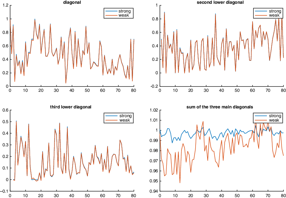
Figure 3. Entries of the coefficient matrix on the three diagonals under the two prior specifications, as well as the sum of these three diagonals. Values on the x-axis correspond to the age of interst, which ranges between 0 and 100.
In both cases, the entries of the posterior mean of A are close to, but not exactly equal to 0, except near the main diagonal as well as the two lower, subdiagonals. By comparing the two panels, we can see that as expected, when the strong shrinkage is used, the non-diagonal entries of matrix A are even closer to zero. To dig deeper into the comparison, let us now focus on the entries on the main diagonal, as well as the two subdiagonals immediately below the main diagonal. Their values, as well as their sums, are displayed in Figure 4.
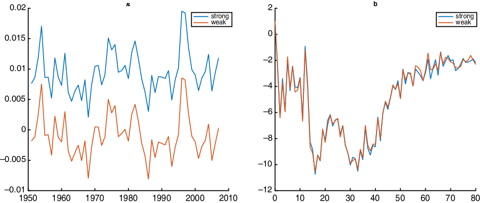
Figure 4. Left panel: posterior trajectory of the latent factor over time in the FAVAR model; right panel: the curve of the associated loading factor across different ages. The blue and orange full lines indicate the specifications with strong and weak shrinkage, respectively.
When the strong shrinkage is used, the sum of the three diagonals is closer to 1 for most ages. This is expected, since this equality is satisfied in the benchmark, Li and Lu model. Thus by relaxing the sparsity constraint of matrix A, the FAVAR model provides more flexibility and improves the fit and the precision of forecast. One caveat of our results is that even though the entries of A are shrunk towards the benchmark model, since the entries of this latter have not been smoothed, this strong variation is somehow inherited by the posterior distribution of A, as is illustrated by the erratic curve of the three diagonals in Figure 4. Note, however, that a similar downside can also exist, if any other VAR models including those involving frequentist shrinkage algorithm (see e.g., Guibert et al., Reference Guibert, Lopez and Piette2019). Note, however, that this downside can be mitigated in several ways. First, as suggested in Li and Lu (Reference Li and Lu2017), we can estimate the Li and Lu model using Ridge regression instead of using OLS so that the prior mean of A is smoother. Alternatively, one might also change the prior covariance matrix of the coefficient matrix A. More precisely, instead of assuming its entries to be mutually independent in the Minnesota prior, we could specify its distribution diagonal by diagonal taking different diagonals mutually independent. Then, within each diagonal, one could assume that the joint distribution of the entries follows Gaussian distribution, with a high correlation between neighbouring terms to ensure smoothness. Since A’s distribution remains Gaussian, the MCMC algorithm described above can be easily adapted to this new specification.
Posterior factor component. In the left panel of Figure 5, we display the posterior mean of the factor path $(\kappa_{t})$
, under either the strong or the weak shrinkage prior. We exclude
$(\kappa_{t})$
, under either the strong or the weak shrinkage prior. We exclude $\kappa_{1}$
, since it is set to be zero.
$\kappa_{1}$
, since it is set to be zero.

Figure 5. Posterior bivariate density of $\gamma_{2}$
and
$\gamma_{2}$
and $\rho(A)$
under the four prior specifications: left panel: the model with strong shrinkage prior; right panel: the model with weak shrinkage prior.
$\rho(A)$
under the four prior specifications: left panel: the model with strong shrinkage prior; right panel: the model with weak shrinkage prior.
Table 1. In-Sample and out-of-Sample MSE.

We can see that first, process $(\kappa)$
seems to have a stationary path.Footnote 13 Second, its path does not differ too much between the two models with strong and weak shrinkage, echoing the comparable forecasting performance shown in Table 1.
$(\kappa)$
seems to have a stationary path.Footnote 13 Second, its path does not differ too much between the two models with strong and weak shrinkage, echoing the comparable forecasting performance shown in Table 1.
Joint posterior distribution. Let us now focus on the joint posterior distribution of regression coefficient $\gamma_{2}$
and the spectral radius
$\gamma_{2}$
and the spectral radius $\rho(A)$
of A, that is the maximum absolute eigenvalue of the eigenvalues of A. These two parameters are important, since in a frequentist setting, their values are essential in determining the long-term dynamics of process
$\rho(A)$
of A, that is the maximum absolute eigenvalue of the eigenvalues of A. These two parameters are important, since in a frequentist setting, their values are essential in determining the long-term dynamics of process $(y_{t})$
. Indeed,
$(y_{t})$
. Indeed,
-
If
$\gamma_{2}$
is between 0 and 1, then process
$(\kappa_{t})$
is stationary. Then


-
− if the eigenvalues of A are all smaller than 1, then process
$(y_{t})$
is also stationary. -
− if some of the eigenvalues of A are equal to 1, then
$Id-A$
is of reduced rank and some of the components of
$y_{t}$
are integrated. Then there might exists co-integration relationships, and the co-integration vectors are the left eigenvectors of matrix
$Id-A$
. -
− if some of the eigenvalues of A are larger than 1, then some of the components of
$y_{t}$
are geometrically explosive.


-
If instead
$\gamma_{2}$
is equal to 1, that is process
$(\kappa_{t})$
is integrated, then:


-
− if the eigenvalues of A are all smaller than 1, then process
$(y_{t})$
is integrated of order 1 and no co-integration relationship exists. -
− if some of the eigenvalues of A are equal to 1, then process
$(y_{t})$
is integrated of order 2.


Figure 6 below plots the joint density of $\gamma_{2}$
and
$\gamma_{2}$
and $\rho(A)$
for each of the two prior specifications.
$\rho(A)$
for each of the two prior specifications.

Figure 6. US male mortality for age.
In both panels, $\gamma_{2}$
is close to zero. In other words, the US data strongly suggest the necessity of the VAR component to capture the decreasing trend of mortality, as compared to the well-established LC model. It is worth noting, however, that the median of the distribution of
$\gamma_{2}$
is close to zero. In other words, the US data strongly suggest the necessity of the VAR component to capture the decreasing trend of mortality, as compared to the well-established LC model. It is worth noting, however, that the median of the distribution of $\rho(A)$
tends to be larger than 1. This “counter-intuitive” feature can be explained by several of the following reasons. First, if we consider an unconstrained VAR model for this dataset, since the dimension of vector
$\rho(A)$
tends to be larger than 1. This “counter-intuitive” feature can be explained by several of the following reasons. First, if we consider an unconstrained VAR model for this dataset, since the dimension of vector $y_{t}$
,
$y_{t}$
, $d=100$
, is larger than
$d=100$
, is larger than $T=79$
, the coefficient matrix A is not identified and hence cannot be estimated using OLS. In other words, we can find values of A such that an unconstrained VAR model produces perfect fit. This is the standard
$T=79$
, the coefficient matrix A is not identified and hence cannot be estimated using OLS. In other words, we can find values of A such that an unconstrained VAR model produces perfect fit. This is the standard $``p>n$
” issue in statistics and could be potentially solved in several ways. In our approach, even though this issue is mitigated by putting a Bayesian prior on A, this solution remains imperfect. First, we could follow the literature and limit the age range of our data to, say, 50,…,100, so that d becomes smaller tan T. Second, we could consider even stronger shrinkage prior, so as to penalise the deviation of A from its benchmark value, whose spectral radius is equal to 1. Moreover, in order to force the spectral radius of A to be exactly equal to 1 so that we get exact co-integration relationships, we could also use other types of priors, such as the sum of coefficient prior proposed by Sims and Zha (Reference Sims and Zha1998) and used in Njenga and Sherris (Reference Njenga and Sherris2020). This latter extension, however, is out of the scope of the current paper and will be left for future research. Note, also, that the fact that the median of
$``p>n$
” issue in statistics and could be potentially solved in several ways. In our approach, even though this issue is mitigated by putting a Bayesian prior on A, this solution remains imperfect. First, we could follow the literature and limit the age range of our data to, say, 50,…,100, so that d becomes smaller tan T. Second, we could consider even stronger shrinkage prior, so as to penalise the deviation of A from its benchmark value, whose spectral radius is equal to 1. Moreover, in order to force the spectral radius of A to be exactly equal to 1 so that we get exact co-integration relationships, we could also use other types of priors, such as the sum of coefficient prior proposed by Sims and Zha (Reference Sims and Zha1998) and used in Njenga and Sherris (Reference Njenga and Sherris2020). This latter extension, however, is out of the scope of the current paper and will be left for future research. Note, also, that the fact that the median of $\rho(A)$
is larger than 1 does not necessarily mean that the prediction. Note, also, that since the operator
$\rho(A)$
is larger than 1 does not necessarily mean that the prediction. Note, also, that since the operator $\rho(\cdot)$
is nonlinear, the spectral radius of the posterior mean of A is different from the mean of
$\rho(\cdot)$
is nonlinear, the spectral radius of the posterior mean of A is different from the mean of $\rho(A)$
. In particular, the latter is larger than 1, whereas the former is equal to 0.9951 or 1.0031, depending on the (strong or weak) shrinkage. In other words, on average, the future evolution of the mortality do not explode. This feature is further confirmed by the fan plots of the probability forecasts.
$\rho(A)$
. In particular, the latter is larger than 1, whereas the former is equal to 0.9951 or 1.0031, depending on the (strong or weak) shrinkage. In other words, on average, the future evolution of the mortality do not explode. This feature is further confirmed by the fan plots of the probability forecasts.
Table 2. In-sample and out-of-sample MSE.

Predictive density. Figure 7 reports the fan plots of the density forecast of the log-mortality for two ages (55 and 65 years). We do so for three models (LC, Li and Lu, and FAVAR). For each model, we simulate a large number of future mortality scenarios and take the 16 and 84 percentiles as the confidence bounds of the forecasts.Footnote 14

Figure 7. Evolution of the log-mortality over time at ages 20, 40, 60 and 80 years for the French male population.
The decreasing trend of the mortality predicted by the model seems to be steady, rather than accelerating. Note, also that we observe a significant jump-off for the first year of forecasting ( $t=2009$
), due to the fact that for the last year of the sample size (
$t=2009$
), due to the fact that for the last year of the sample size ( $t=2008$
), the fitted mortality rate is not equal to the historical value. This jump-off error, however, is well documented in the literature, see for example, Lee and Miller (Reference Lee and Miller2001).
$t=2008$
), the fitted mortality rate is not equal to the historical value. This jump-off error, however, is well documented in the literature, see for example, Lee and Miller (Reference Lee and Miller2001).
We end this subsection on a few comments about the time and age dimension, as well as the forecast horizon. In the above analysis, we have chosen all ages between 0 and 100 years and used data between 1930 and 2007 for estimation. The choice of such a large age dimension is motivated by our desire to demonstrate the ability of the Bayesian model to tackle the high-dimensional “ $p>n$
” issue. In some actuarial applications, it might be more useful to focus on post-retirement age, while at the same time focus on data after the WW2. In Appendix C, we propose an analysis in which we randomly choose the age and time dimension and compare the performance of our model against its two competitors (LC and Li and Lu) when these random sample are picked. Similarly, the forecast horizon has previously been set to 10 years, which correspond to the length of the data we left out for backtesting. Because this horizon might seem rather short for some actuarial applications, in Appendix D, we also report the forecast of the log-mortality for a horizon of 50 years.
$p>n$
” issue. In some actuarial applications, it might be more useful to focus on post-retirement age, while at the same time focus on data after the WW2. In Appendix C, we propose an analysis in which we randomly choose the age and time dimension and compare the performance of our model against its two competitors (LC and Li and Lu) when these random sample are picked. Similarly, the forecast horizon has previously been set to 10 years, which correspond to the length of the data we left out for backtesting. Because this horizon might seem rather short for some actuarial applications, in Appendix D, we also report the forecast of the log-mortality for a horizon of 50 years.
4.2. French male data
In this subsection, we will replicate the same analysis as for US males and compare the new results with those obtained previously.
Data. Similar as for the US data, we use the French data (from 1950 to 2008). We partition our data into the training set (from 1950 to 2007) and the validation set (from 2008 to 2018) and use the same age range (0–80 years) as before. Figure 8 is the analogue of Figure 1 and provides the evolution of the log-mortality rates at four different ages.

Figure 8. The dynamic time trend and its age specific responses.
Remind that for the US data, the difference between the four different series tends to be stationary over time. This does not seem to be the case for the French data, since the mortality rates at younger ages (20 and 40 years) decreases at a much higher pace than those at higher ages (60 and 80 years). Since one of the key consequences of the Li and Lu (Reference Li and Lu2017) model is the stationarity of these log-mortality differentials, this pattern suggests that this latter model might be much less suitable for the French male mortality data. This intuition will also be quantitatively confirmed later on in Table 2.
Prior specification and model estimation. Given the likely inadequacy of Li and Lu (Reference Li and Lu2017)’s model for the French data, we will slightly change the prior specification of our FAVAR model. More precisely, instead of setting the prior mean of matrix A to be the coefficient matrix of the Li and Lu model, we will simply follow the standard Minnesota prior, by setting $\mathbb{E}[A]$
to be the identity matrix. Then we also consider two prior specifications, corresponding to strong and weak shrinkages. Compared to the US data (
$\mathbb{E}[A]$
to be the identity matrix. Then we also consider two prior specifications, corresponding to strong and weak shrinkages. Compared to the US data ( $T=79$
), our T is much larger now (
$T=79$
), our T is much larger now ( $T=193$
). Thus, we will be able to loosen the tightness of the prior. As a consequence, both the strong and weak shrinkages proposed below are weaker than their counterparts used for the US data:
$T=193$
). Thus, we will be able to loosen the tightness of the prior. As a consequence, both the strong and weak shrinkages proposed below are weaker than their counterparts used for the US data:
-
strong shrinkage, with small values of
$c_{2}$
and
$c_{3}$
:
$c_{1}=100,c_{2}=0.2^{2.35},c_{3}=0.1^{2.35}$
-
weak shrinkage, with larger values of
$c_{2}$
and
$c_{3}$
:
$c_{1}=100,c_{2}=0.2^{2},c_{3}=0.1^{2}.$


Finally, the values of the other hyperparameters are set as the same as for US males. Table 2 below, which is the analogue of Table 1, reports both in-sample and out-of-sample MSE of the four models.
As expected, the Li and Lu model leads to moderate improvement in terms of the in-sample fit and short-term (one-year-ahead or five-year-ahead) forecasting compared to the LC model but is quite unsatisfactory when we increase the forecast horizon to 10 years. On the other hand, we can see that both the strong and weak FAVAR model deliver much better results, both in sample and out-of-sample.
The dynamic time trend. Let us now focus on the filtered trajectory of $(\kappa_{t})$
. One remarkable difference between Figure 9 (for French data) and Figure 5 (for US data) is that there are several large spikes in Figure 9, mainly during the two World Wars as well as around the French (February) revolution of 1848. This confirms the usefulness of augmenting the standard VAR model with a common factor, especially for the sake of capturing extreme mortality events.
$(\kappa_{t})$
. One remarkable difference between Figure 9 (for French data) and Figure 5 (for US data) is that there are several large spikes in Figure 9, mainly during the two World Wars as well as around the French (February) revolution of 1848. This confirms the usefulness of augmenting the standard VAR model with a common factor, especially for the sake of capturing extreme mortality events.
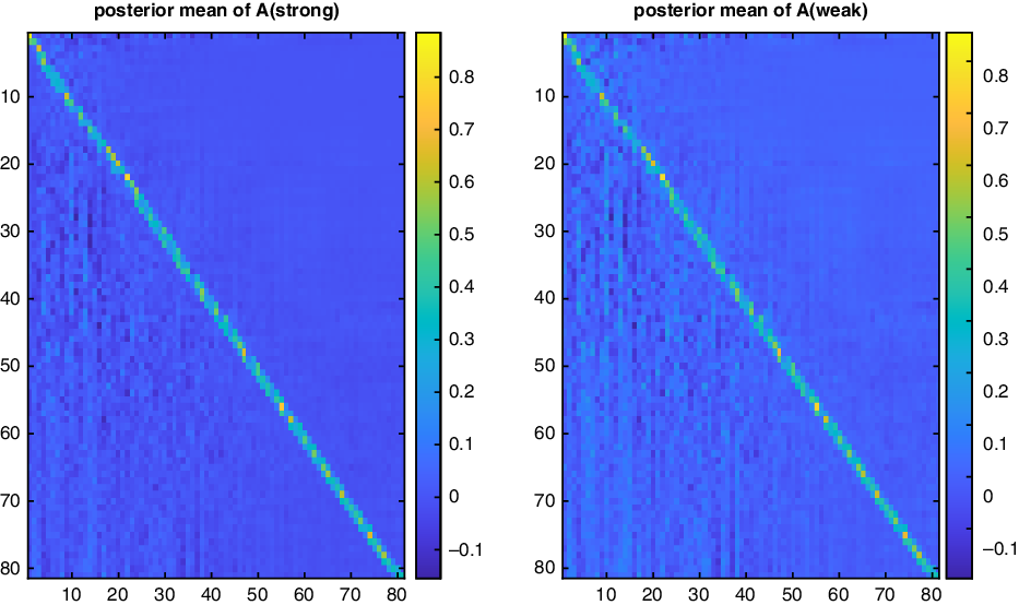
Figure 9. Heat map of the posterior mean of matrix A for French male population. Left panel: the posterior mean with strong shrinkage prior; Right panel: the posterior mean with weak shrinkage prior.
The Posterior VAR component. Figure 10 below is the analogue of Figure 6 for French male population.

Figure 10. The posterior mean of $A_{i,0}$
and
$A_{i,0}$
and $A_{i,19}$
for different ages i.
$A_{i,19}$
for different ages i.
Compared to the US data, more entries off the main diagonals are significant for the French population. In particular, the entries on the first column of the posterior mean of A indicate a strong Granger causality between infant mortality and mortality at other age groups. In Figure 10, we plot the posterior mean of $A_{i,0}$
and
$A_{i,0}$
and $A_{i,19}$
, say, for i varying between 0 and 100. The value of
$A_{i,19}$
, say, for i varying between 0 and 100. The value of $A_{i,19}$
is negligible except for its neighbouring age groups. In contrast, the value of
$A_{i,19}$
is negligible except for its neighbouring age groups. In contrast, the value of $A_{i,0}$
is generally non-zero and increases in i. This dependence of the mortality rate of the elderly population on infant mortality might be explained by the fact that both the infant and the elderly population’s mortality improvement are heavily dependent on that of the health care services. This feature would not have been uncovered, had we restricted ourselves to the Li and Lu model or its related extensions (see Feng et al., Reference Feng, Shi and Chang2021).
$A_{i,0}$
is generally non-zero and increases in i. This dependence of the mortality rate of the elderly population on infant mortality might be explained by the fact that both the infant and the elderly population’s mortality improvement are heavily dependent on that of the health care services. This feature would not have been uncovered, had we restricted ourselves to the Li and Lu model or its related extensions (see Feng et al., Reference Feng, Shi and Chang2021).
Figure 11 reports the values on three diagonals of the posterior mean of A. Remind that the prior mean of A is equal to the identity matrix, corresponding to a sum of exactly 1 of these three diagonals. In contrast, the lower right panel of Figure 12 suggest that a posteriori, this sum is quite far from being equal to 1. This means that the underlying benchmark model $y_{t}=y_{t-1}+b\kappa_{t}+\epsilon_{t}$
is not appropriate for the French data.Footnote 15 But thanks to the larger sample size, the algorithm has been able to “learn” from the data and managed to find a more appropriate form for A.
$y_{t}=y_{t-1}+b\kappa_{t}+\epsilon_{t}$
is not appropriate for the French data.Footnote 15 But thanks to the larger sample size, the algorithm has been able to “learn” from the data and managed to find a more appropriate form for A.

Figure 11. Entries of the coefficient matrix on the three diagonals under the two prior specifications, as well as the sum of these three diagonals.

Figure 12. Heat map of the joint histogram of $\rho(A)$
and
$\rho(A)$
and $\gamma_{2}$
. Left panel: the result with strong prior; right panel: the result with weak prior.
$\gamma_{2}$
. Left panel: the result with strong prior; right panel: the result with weak prior.
Posterior Joint distribution of $\rho(A)$
and
$\rho(A)$
and $\gamma_{2}$
. Figure 13 plots the joint posterior distribution of
$\gamma_{2}$
. Figure 13 plots the joint posterior distribution of $\rho(A)$
and
$\rho(A)$
and $\gamma_{2}$
.
$\gamma_{2}$
.

Figure 13. French data forecast.
For this model, the maximum eigenvalue for the posterior mean of A is 1.0001 and 1.0088, respectively, in the two prior set-ups.
Predictive density. Finally, we display the predictive density of the log-mortality rates in the next 10 years, for ages 55 and 65 years, respectively.
Finally, in Appendix D, we report also the prediction of the log-mortality under our model with a foreast horizon of 50 years.
5. Conclusion
This paper has introduced the (Bayesian) FAVAR model into the mortality forecasting literature. This model is a flexible extension of both DFM (LC and CBD) and VAR models. In particular, it extends the sparse VAR model proposed in Li and Lu (Reference Li and Lu2017) by (i) making the coefficient matrix flexible instead of sparse; (ii) adding an extra common factor à la LC model. Furthermore, we have carefully explained the choice of the prior distribution and a straightforward MCMC algorithm to estimate this parameter-rich model and derive the parameter estimate’s uncertainty. Finally, we have illustrated the flexibility of our Bayesian approach through the US and French mortality data by considering different prior specifications.
Note that our model has a slight difference from other FAVAR models in the macroeconomics literature. Indeed, in these latter models, the unobserved factor(s) $(\kappa_{t})$
is often further related to other (possibly multivariate) variables
$(\kappa_{t})$
is often further related to other (possibly multivariate) variables $x_{t}$
not included in the “main” variable of interest
$x_{t}$
not included in the “main” variable of interest $y_{t}$
, through a linear relationship of the type:
$y_{t}$
, through a linear relationship of the type:
 \begin{equation}x_{t}=My_{t}+c\kappa_{t}\end{equation}
for suitable matrices M and c. Such a specification, along with equation (1), allows the macroeconomist to extract extra information from the “auxiliary” process $(x_{t})$
to predict
$(x_{t})$
to predict $y_{t}$
better. In our model, however, the factor brings in no extra information other than what is already contained in the mortality rates. It has been shown in the mortality literature (see, e.g., Boonen and Li, Reference Boonen and Li2017) that the inclusion of economic variables can potentially be beneficial to the forecasting performance.Footnote 16 As a consequence, a natural avenue for future research would be to expand our model and include economic variables
$y_{t}$
better. In our model, however, the factor brings in no extra information other than what is already contained in the mortality rates. It has been shown in the mortality literature (see, e.g., Boonen and Li, Reference Boonen and Li2017) that the inclusion of economic variables can potentially be beneficial to the forecasting performance.Footnote 16 As a consequence, a natural avenue for future research would be to expand our model and include economic variables $x_{t}$
. This would also be particularly relevant if the modeller were interested in a joint projection of economic and demographic scenarios.
$x_{t}$
. This would also be particularly relevant if the modeller were interested in a joint projection of economic and demographic scenarios.
Acknowledgement
The authors wish to thank Profs. Farshid Vahid, Athanasios Pantelous and Jackie Li for helpful comments. Yang Lu thanks NSERC (RGPIN-2021-04144 and DGECR-2021-00330) for financial support. Part of the work is conducted when Lu was working at University of Paris 13.
Appendix A. The expression of the likelihood function
Let us rewrite the logged joint likelihood (3.8) into:
 \begin{align}\log l(\mathbf{Y,\boldsymbol{\kappa}}|\theta)= & -\frac{T-1}{2}\sum_{x=x_{0}}^{x_{0}+d-1}\log(\sigma_{x}^{2})\nonumber \\[5pt] &\quad -\frac{T-1}{2}\log(\sigma_{\eta}^{2})-\frac{1}{2}trace\left(\left[Y-X\alpha-\boldsymbol{\kappa}b'\right]\Sigma^{-1}\left[Y-X\alpha-\boldsymbol{\kappa}b'\right]\right) \\[5pt] & \quad-\frac{1}{2\sigma_{\eta}^{2}}\left[\left(\mathbf{I}_{T-1}-\gamma_{2}H\right)\boldsymbol{\kappa}-\gamma_{1}\mathbf{1}_{T-1}\right]'\left[\left(\mathbf{I}_{T-1}-\gamma_{2}H\right)\boldsymbol{\kappa}-\gamma_{1}\mathbf{1}_{T-1}\right],\nonumber\end{align}
where the $T\times T$
square matrix H is such that
$T\times T$
square matrix H is such that $H\boldsymbol{\kappa}=[0,\kappa_{2},...,\kappa_{T-1}]'.$
Then by integrating out the Gaussian process
$H\boldsymbol{\kappa}=[0,\kappa_{2},...,\kappa_{T-1}]'.$
Then by integrating out the Gaussian process $\boldsymbol{\kappa}$
, we can simplify Equation (3.7) into:
$\boldsymbol{\kappa}$
, we can simplify Equation (3.7) into:
 \begin{equation}\log\left(f(\mathbf{Y}|\theta)\right)=-\frac{1}{2}\log(2\pi|\boldsymbol{\Sigma_{\boldsymbol{{Y}}}}|)-\frac{1}{2}vec(Y-X\alpha-V)'\boldsymbol{\Sigma_{\boldsymbol{{Y}}}}^{-1}vec(Y-X\alpha-V),\end{equation}
where matrix $\Sigma_{Y}$
is given by:
$\Sigma_{Y}$
is given by:
 \begin{align*}\boldsymbol{\Sigma_{\boldsymbol{{Y}}}}= & \Sigma\otimes\mathbf{I}_{T-1}+\sigma_{\eta}^{2}bb'\otimes\left[\left(\mathbf{I}_{T-1}-\gamma_{2}H\right)^{\prime}\left(\mathbf{I}_{T-1}-\gamma_{2}H\right)\right]^{-1}\\[5pt]V= & \left[\left(\mathbf{I}_{T-1}-\gamma_{2}H\right)'\left(\mathbf{I}_{T-1}-\gamma_{2}H\right)\right]^{-1}\left(\mathbf{I}_{T-1}-\gamma_{2}H\right)^{\prime}\mathbf{1}_{T-1}b'.\end{align*}
Appendix B. Checking algorithm convergence using traceplot
To demonstrate the convergence of the Gibbs sampler, we resort to traceplots. For each component of the vector of parameters, the traceplot reports the evolution of the simulated values of this parameter across different MCMC iterations. For illustration purpose, in Figure 1, we only choose four components from the vector of parameters: $a_{1}$
(northwest panel),
$a_{1}$
(northwest panel), $b_{1}$
(northeast panel),
$b_{1}$
(northeast panel), $\gamma_{1}$
and
$\gamma_{1}$
and $S_{1}$
.Footnote 17 In our estimation procedure, the parameter is sampled for a total of 1000 times, hence in Figure 13, the x-coordinate is
$S_{1}$
.Footnote 17 In our estimation procedure, the parameter is sampled for a total of 1000 times, hence in Figure 13, the x-coordinate is $s=1,...,1000$
. For instance, the northwest panel indicate that most of the simulated values of
$s=1,...,1000$
. For instance, the northwest panel indicate that most of the simulated values of $a_{1}$
lie between 0.5 and
$a_{1}$
lie between 0.5 and $-0.5$
. Generally speaking, we can reasonably say that the MCMC algorithm has converged, if there is sufficient variation of the parameters across different iterations. From the four panels of Figure 1, we can see that this is indeed the case for each of the parameters.
$-0.5$
. Generally speaking, we can reasonably say that the MCMC algorithm has converged, if there is sufficient variation of the parameters across different iterations. From the four panels of Figure 1, we can see that this is indeed the case for each of the parameters.

Figure B.1: Traceplot of 1000 MCMC samples post burning for US male mortality data for age 50–101 years and year 1950–2007.
Appendix C. Impact of the choice of age range and sample period on estimation
Let us now test the robustness of our proposed model against LC, VARFootnote 18 Li&Lu, as well as the functional data (henceforth, FDM) model of Hyndman and Ullah (Reference Hyndman and Ullah2007), for different choices of age groups and sampling periods. We focus on the US and French male mortality data for illustration purposes. We replicate the estimation/forecasting procedure a total of 100 times. These replications differ in the sample period and range of age retained for estimation purposes. More precisely,
-
for the sample period, we randomly select the sample from
$1933+D$
to 2007 where the random variable D (for delay) follows
$D\sim bin(70,0.3)$
. In other words, the average sample size is 2007-1933+1-70(0.3)=53 across the 100 replications. -
for the age of range retained for estimation, we randomly select
$N_{x}=30+bin(30,0.5)$
different age groups from age 0 to 100 years, which implies that on average, we have 45 ages cohorts.


For each replication, we compute the RMSE of the four models when it comes to in-sample, 1-year-ahead, 5-year-ahead and 10-year-ahead forecast, respectively.
US male population
Table C.1 below reports the RMSE for US male population for the five models.
Table C.1: In-Sample/Out-of-Sample for US Male population. The four numbers presented are RMSE of in-sample fit, forecast of horizon 1, 5 and 10 periods.
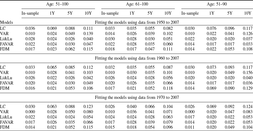
We can see that the Hyndman and Ullah (Reference Hyndman and Ullah2007) FDM model provides good in-sample fit but is not very competitive when it comes to out-of-sample forecast. The same remark applies to the VAR model, which likely suffers from some degree of over-fitting. The FAVAR model, on the other hand, has smaller in-sample fit compared to its major competitors LC and Li and Lu, while outforming these two latters in terms of out-of-sample performance.
Appendix D. Long-term forecast
In the main text, the forecast horizon has been fixed to a maximum of 10 years. In this Appendix, let us project the log-mortality to a longer horizon using the FAVAR model. For both US male and French male populations, we use data from 1950 onwards with age group 50–91 years and project the mortality from 2019 to 2068, which amounts to a total of 50 periods. The realised log-mortality and the central forecast (benchmarked against the LC) are plotted in the Figures D.1 and D.2 below for US male and French male populations, respectively.

Figure D.1: Long-term mortality forecast for US male population for four different ages. Dotted lines are historical mortality rates; full lines are point forecasts given by the FAVAR model; dashed lines are the point forecasts given by the LC model.

Figure D.2: Long-term mortality forecast for French male population for four different ages. Dotted lines are historical mortality rates; full lines are point forecasts given by the FAVAR model; dashed lines are the point forecasts given by the LC model.
In both cases, we observe quasi-linear improvement of the log-mortality at various ages. We can also remark that the slow down of the mortality improvement observed among younger ages in both US and France is projected to propagate into higher ages progressively in the future, creating a sort of “wave.” This can be interpreted as the cohort effect (Li and Lu, Reference Li and Lu2017), or the “heat wave” effect (Li and Liu, Reference Li and Liu2020).
Table D.1: In-Sample/Out-of-Sample for French Male populations. The four numbers presented are RMSE of in-sample fit, forecast of horizon 1, 5 and 10 periods.


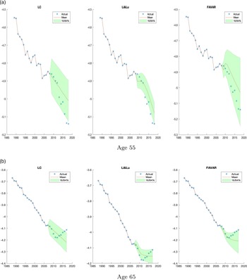


 Open access