


Impact Statement
Fiducial markers such as gold nanoparticles are often added to samples in transmission electron tomography to assist in image alignment prior to 3D reconstruction. Particularly for thick samples, tracking of individual fiducials often fails due to low contrast. ClusterAlign is a software that follows the structure of fiducial clusters, rather than individuals, to serve for alignment of the tilt series and 3D reconstruction.
1. Introduction
Electron tomography offers a powerful set of tools to reveal cellular anatomy in three dimensions. The most popular implementation is that of tilt tomography in the transmission microscope. A set of 2D projection images is recorded, from which a 3D volume representation is reconstructed by one of the available algorithms, which include weighted back projection, direct Fourier inversion, and iterative techniques. An essential intermediate step is that of aligning the 2D images to approximate the ideal rotation of a rigid body around a unique tilt axis. In practice, the mechanical mechanism of rotation always introduces some shifts or drift that must be corrected by translation of the images. Additionally, electron-optical distortions as well as geometric distortions due to beam exposure may need to be corrected for a successful reconstruction. In order to facilitate the alignment, high contrast nanoparticles such as colloidal gold are often distributed over the specimen in order to assist in correcting or compensating these faults. Tracking the nanoparticles from tilt to tilt across the series serves to establish precisely the tilt axis orientation and to bring the 2D images into alignment around it. As manual tracking is tedious, a number of algorithms have been developed for automatic detection and tracking of the fiducial markers(Reference Amat, Moussavi, Comolli, Elidan, Downing and Horowitz 1 –Reference Lawrence, Bouwer, Perkins and Ellisman 6 ). Despite significant advances in software, precise tracking of fiducials can still be difficult to automate, however. Alternatively, a number of fiducial-less alignment algorithms have been developed(Reference Castaño-Díez, Scheffer, Al-Amoudi and Frangakis 7 –Reference Noble and Stagg 13 ). A recent and successful addition is AreTomo, which is based on successive matching of projections from partial reconstruction to align the tilt series(Reference Zheng, Wolff and Greenan 14 ). In such cases, added fiducials may be used as a diagnostic of the alignment quality and indicator of the need for follow-up refinement. The widespread adoption of tomographic acquisition in batch mode accentuates the need for unattended alignment as a first step in data interpretation.
The introduction of scanning transmission electron microscopy(Reference Hohmann-Marriott, Sousa and Azari 15 , Reference Wolf, Houben and Elbaum 16 ), as well as soft X-ray imaging(Reference Do, Isaacson, McDermott, Le Gros and Larabell 17 –Reference Kapishnikov, Berthing and Hviid 19 ) modalities, has expanded the range of specimen thickness accessible to cryo-tomography(Reference Elbaum 20 ). The specimen can no longer be considered a thin slab when its thickness may typically reach half the lateral field of view. This introduces specific issues for alignment. The pileup of features in a thick specimen flattens the contrast overall, hindering the effectiveness of fiducial-less alignment, and on the other hand small fiducials may be poorly resolved in transmission through the thick material. This problem often becomes acute at high tilt angles where the projected thickness increases, and moreover, high-contrast features in the sample itself may hide or shadow the fiducials over a limited range of tilt angles. Thus, it becomes difficult even to identify individual particles reliably in every projection and to track the particles across large gaps in tilt views. One popular approach is to build a model of the rotation that can predict the projected position of individual fiducial markers, allowing the user to accept or correct the prediction so as to fill the gaps(Reference Mastronarde and Held 5 –Reference Kremer, Mastronarde and McIntosh 21 ). Other approaches generate overlapping chains of landmarks, each covering a part of the tilt range(Reference Chen, Bell, Shi, Sun, Wang and Ludtke 8 –Reference Messaoudi, Boudier, Sorzano and Marco 12 ), or make use of a local invariant criterion(Reference Han, Wang, Liu, Sun and Zhang 3 ). Further developments are underway, with an emphasis on unattended operation to support the ever-increasing throughput of data acquisition.
Here we offer a complementary strategy to that of following individual fiducial markers. We identify extended clusters that transform geometrically between each of the tilted projections and a single reference view at low tilt angle, where visibility is optimal. Essentially, these are the subsets of fiducials that lie at similar height perpendicular to the view direction, and whose distributions transform with the cosine of the tilt angle. Multiple such clusters may be found and may even overlap, for example, when particles are located on two sides of a slab. The verified cluster vertices are then used as fiducials, rather than the locations of individual particles. Thus, we avoid the need to follow the same particle sequentially from tilt to tilt, and the cluster location is inherently robust to disappearance of individual particles. The relative motions of multiple identified cluster vertices are then used as fiducial markers to constrain the precise position and angle of the tilt axis by least squares fitting. The program can output the list of tracked fiducials in a format compatible with IMOD(Reference Mastronarde and Held 5 ) or Tomoalign(Reference Fernandez, Li, Bharat and Agard 9 ), a stack containing the aligned tilt series, or a completed 3D reconstruction. In addition, a text file reports the transformations and error estimates generated during the processing.
Alignment error is primarily translational and thus expected to be corrected by solving for Δx,Δy shifts of the image, but the algorithm is tolerant to moderate global in-plane and out of plane rotations. Note that clusters are defined by a common height with respect to the tilt axis and need not be composed of apparently adjacent fiducials in any given projection. Thus, the aim of the software is to optimize translational alignments under conditions of problematic fiducial visibility without manual intervention.
2. Method
2.1. Software features
A flowchart of the processing appears in Figure 1. The workflow involves three major stages: fiducial particle identification, cluster assignment, and rigid body fitting of the tilt axis. Compatibility is maintained with IMOD file formats and conventions. The software is written in C#, makes use of the EMGU/OpenCV library,(Reference Bradski 22 , 23 ) and is available as open source under the GNU-GPLv3 license (see Data Availability Statement). Processing 800 fiducials in a tilt series of 57 frames of 2k × 2k frame size requires 4 min on a 24-core Intel Xeon-based computer, and the reconstruction using Nvidia RTX 3060 GPU with binning of 2 takes an additional 4 min.
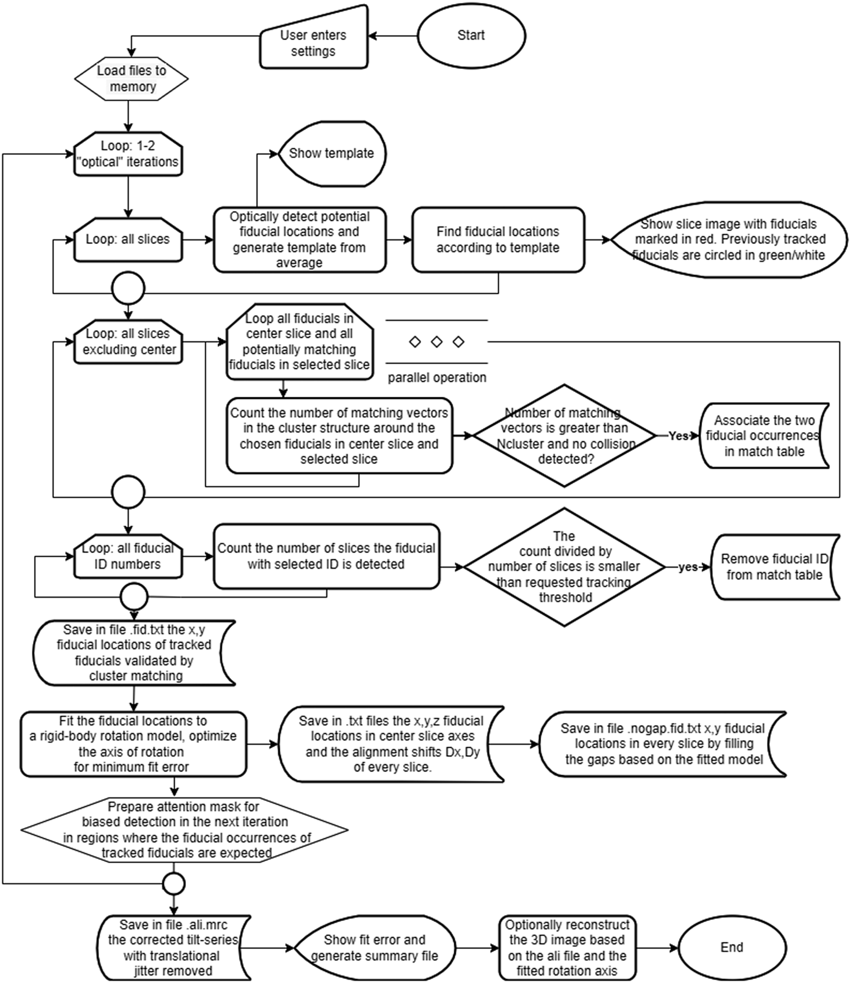
Figure 1. A flowchart of the ClusterAlign processing workflow.
The key input parameters appear in Table 1 and the user interface in Figure 2. Most parameters are self-explanatory. Significance of those related to cluster assignment is explained below. Practical details appear in the user manual (see Data Availability Statement).
Table 1. Settings.


Figure 2. The ClusterAlign user interface. See the user manual for more information.
The software supports optional loading of external fiducial files and pre-aligned stacks for refinement, optional reconstruction in single or dual axis, and loading of an attention mask for special uses explained in the user manual. There is also support for cosine sampling tomograms, which can be acquired by varying the aspect ratio of the scan pattern(Reference Seifer, Houben and Elbaum 24 ).
The user may choose to run the analysis in two iterations to enhance precisions. The information that is carried between iterations is global and does not include particular trajectories. The knowledge gained in the first iteration is used to update the tracking threshold, to generate attention maps, and to determine fiducial size. The predicted locations of fiducial according to a rigid body model are displayed during the second iteration.
The output of the program is a text-based fiducial list of the form used by Tomoalign (.fid.txt), which can be converted to the binary IMOD format (.fid) using the command point2model. An aligned tilt series is generated either by imposing only translation corrections without adjustment of the tilt axis (_jali.mrc), or in standard form (_ali.mrc) globally aligned with tilt axis vertical and centered. Optionally, the package can output a Simultaneous Iterative Reconstruction Technique (SIRT) reconstruction based on the Astra toolbox(Reference Palenstijn, Batenburg and Sijbers 25 , Reference van Aarle, Palenstijn and De Beenhouwer 26 ), which corresponds to the exact fitted rotation axis. (This option is available only on computers equipped with GPU and Matlab.) The default generated tilt series (_jali.mrc) best matches our Matlab tomogram reconstruction using rotation axis properties found in file (.output.txt), while the standard form is intended for compatibility with other reconstruction software such as IMOD or tomo3d(Reference Agulleiro and Fernandez 27 ). No attempt is made to optimize view angles that deviate from the mechanical tilts, nor local alignments to compensate for specimen distortion. Optimizations such as focused local alignment or global distortion corrections may be performed in other dedicated software such as Tomoalign(Reference Fernandez, Li, Bharat and Agard 9 ), EMClarity(Reference Himes and Zhang 10 ), or constrained reconstruction model(Reference Han, Li, Yang, Zhang and Gao 28 ). Furthermore, the Astra toolbox can reconstruct from several rotation axes at once. We provide a Matlab module for dual axis reconstruction that can be used after separate alignment of each tilt series in ClusterAlign. The method involves rotating the second series by 90° and passing to Astra the 3D center coordinates of each tilt series (example is shown in the Supplementary Materials).
2.2. Particle localization
Detection and localization of particles is an initial step before the actual cluster analysis. The locations of particles are found based on template matching using an average generated from the measured data, an approach that has been used in RAPTOR(Reference Amat, Moussavi, Comolli, Elidan, Downing and Horowitz 1 ). The main difference from previous works is in the method of threshold calculation and in the way particle candidates are selected to generate a template.
The main distinctive feature that allows initial marking the center of particles is the “convoluted divergence,” which is calculated as follows:
 $$ G(M)\hskip0.35em =\hskip0.35em \sqrt{{({\mathrm{ker}}_x\circledast {\mathrm{\nabla}}_xM)}^2+{({\mathrm{ker}}_y\circledast {\mathrm{\nabla}}_yM)}^2,} $$
where $ {\nabla}_xM $
is the gradient in the x direction of the raw gray image. Similarly
$ {\nabla}_xM $
is the gradient in the x direction of the raw gray image. Similarly $ {\nabla}_yM $
is the gradient for the y direction.
$ {\nabla}_yM $
is the gradient for the y direction. $ {\ker}_x $
denotes a small matrix with nonzero elements over positions of a ring that envelopes the range of possible fiducial particle sizes as entered in the user settings. The values of the nonzero elements are
$ {\ker}_x $
denotes a small matrix with nonzero elements over positions of a ring that envelopes the range of possible fiducial particle sizes as entered in the user settings. The values of the nonzero elements are $ {\left({\ker}_x\right)}_{i,j}\hskip0.35em =\hskip0.35em j/\sqrt{i^2+{j}^2} $
,
$ {\left({\ker}_x\right)}_{i,j}\hskip0.35em =\hskip0.35em j/\sqrt{i^2+{j}^2} $
, $ {\left({\ker}_y\right)}_{i,j}\hskip0.35em =\hskip0.35em i/\sqrt{i^2+{j}^2} $
, where i and j are in reference to the center element of the matrix.
$ {\left({\ker}_y\right)}_{i,j}\hskip0.35em =\hskip0.35em i/\sqrt{i^2+{j}^2} $
, where i and j are in reference to the center element of the matrix. $ (A\hskip0.35em \circledast \hskip0.35em B) $
denotes convolution of A with B.
$ (A\hskip0.35em \circledast \hskip0.35em B) $
denotes convolution of A with B.
The next step is to dilate (i.e., replace pixel values by maxima values of) the image of convoluted divergence, $ G(M), $
using a mask with elements 1 over a filled circle the size of the largest particle expected, and elements 0 outside the circle. The locations where
$ G(M), $
using a mask with elements 1 over a filled circle the size of the largest particle expected, and elements 0 outside the circle. The locations where $ G(M) $
= Dilated
$ G(M) $
= Dilated $ \{G(M)\} $
are the peaks of such spots and are considered as candidate fiducial locations. Although the implementation is different, the detection algorithm bears a resemblance to the radiality transform used in the SRRF fluorescence localization microscopy method(Reference Gustafsson, Culley, Ashdown, Owen, Pereira and Henriques
29
).
$ \{G(M)\} $
are the peaks of such spots and are considered as candidate fiducial locations. Although the implementation is different, the detection algorithm bears a resemblance to the radiality transform used in the SRRF fluorescence localization microscopy method(Reference Gustafsson, Culley, Ashdown, Owen, Pereira and Henriques
29
).
Images that have been pre-aligned by cross-correlation or other means contain data-free margins with a sharp gradient at the edges. The program identifies the margins based on regions with zero values of $ G(M) $
and removes these margins from further processing.
$ G(M) $
and removes these margins from further processing.
For each projection in the tilt series, the raw image M[n] is band pass filtered between spatial periods of 1/3 and 20 of the fiducial size, as defined in the user settings panel. The result after further manipulations is a regularized gray image M†[n]. Regions at the sides of M† that are outside the expected projection of a thin layer in the center tilt are masked since any fiducial found there will not be traceable to one that appears in the center slice.
A threshold of the peaks in M† should determine which of the candidate locations of fiducial particles are to be accepted for the next screening process. The maximum allowed number of peaks is determined by the user-defined “maximum number of fiducials” (NfidMax). Initial threshold is calculated by the triangle type threshold algorithm found in EMGU/OpenCV. Then, M† is temporarily multiplied by a mask of spots around the locations of candidate fiducials and the number of contours is counted using the FindContours function. If the count is larger than the maximum allowed number of fiducials, then the threshold is increased incrementally and the process is repeated until the number of fiducials is reduced to fall within the expected range. If such iterations fail, the threshold is determined based on the histogram of gray levels and the total expected area of fiducials.
In the next step, the average image of potential fiducials is generated based on their selected locations. Since we wish to reduce artifacts at sharp edges, the fiducials are filtered according to isotropy. An identified fiducial is considered sufficiently isotropic for inclusion in the average if the normalized correlation between its image and its transposed image is greater than 0.4. This criterion also filters small clusters of particles from consideration. The average fiducial image serves as a template, which is correlated with M† to generate a map H (using the MatchTemplate function in EMGU/OpenCV of type “correlation-normalized”).
The peaks in the correlation map H are considered the candidates for precise locations of the fiducial particles. In order to select the best candidates counted up to NfidMax, the process of finding the suitable threshold is repeated as described above, this time based on the gray levels of M†2 × H and a mask of the candidate locations convoluted with maximum expected fiducial size. The final locations are selected from those candidate locations according to the threshold.
This rather elaborate protocol achieves a high sensitivity (up to 99%) of nanoparticle detection in the sample, excluding most of the artifacts (false negative expected between 1 and 6%) while optimizing the precision of locations reported for the selected particles.
2.3. Fiducial registration by clusters
With a list of detected particle locations in each projection image, the next step is to track them throughout the tilt series. The conventional approach is to track fiducials that are displaced in a direction perpendicular to the tilt axis in adjacent tilt images, working incrementally through the stack. For thick specimens, this approach is not robust because of the very large displacements observed, and because of the possibility for a tracked particle to disappear behind a dense object in the specimen. We apply here an alternative strategy based on recognition of particle clusters.
Each particle location in every slice is selected as a vertex, from which vectors are drawn to all neighboring particles within the user-defined maximum cluster radius. Vector lengths are normalized in the component perpendicular to the tilt axis by the cosine of the tilt angle. The set of vectors emerging from each vertex is then compared between the tilted images and the common center reference image (see Figure 3). Matches are accepted within a tolerance defined in the user settings, typically to 200% of the average fiducial size. (The tolerance allows for some displacement in the z plane.) When the number of matching vectors is greater than a threshold number NCluster (which may be defined by the user or automatically) the vertex is considered a candidate for tracking of a given fiducial at a given slice. If these candidates are indeed unique and are found in a sufficient number of slices (in terms of a user-defined “tracking threshold”), the vertex fiducials are registered as locations of a bona fide fiducial for tracking. Note that recognition of the vector pattern is robust to translations, so the strategy of comparison between tilted projections and an untilted reference does not require a pre-alignment of the tilt series.

Figure 3. Tracking a fiducial across different projections is based on comparing the normalized vectors pointing from each of the detected particle to the surrounding particles in all possible clusters, and approving the cluster association if a sufficient number of vectors match the corresponding patten in the zero-tilt reference image.
Tracking fiducials is the most demanding task in terms of computation time, so the calculations are handled by multi-threading of several CPU cores. Since the success of pairing depends sometimes on the order of the search, the process is not completely deterministic, and thus we may observe a small variability of results for certain ranges of parameters. In particular, collisions may occur where a given particle may be assigned at different tilts to different clusters. Such collisions are detected and removed in advance of the registration of the matches.
2.4. Rigid body analysis
The goal is to align the images by removing the translational shifts $ \left({\Delta x}_{(n)},{\Delta y}_{(n)}\right) $
in every slice n, which originate in mechanical jitter or optical distortions. Thus, to find the translational shifts it is necessary to fit the available information on the set of fiducial particles p at slice n, (
$ \left({\Delta x}_{(n)},{\Delta y}_{(n)}\right) $
in every slice n, which originate in mechanical jitter or optical distortions. Thus, to find the translational shifts it is necessary to fit the available information on the set of fiducial particles p at slice n, ( $ {x}_{(n)}^p $
,
$ {x}_{(n)}^p $
, $ {y}_{(n)}^p $
), with a model. The model considered for rigid body rotation with shifts is
$ {y}_{(n)}^p $
), with a model. The model considered for rigid body rotation with shifts is
 $$ \left(\begin{array}{c}{x}_{(n)}^p\\ {}{y}_{(n)}^p\\ {}{z}_{(n)}^p\end{array}\right)\hskip0.35em =\hskip0.35em {A}_{\left({\theta}_n\right)}^{\overrightarrow{\omega}}\left(\begin{array}{c}{x}_c^p\\ {}{y}_c^p\\ {}{z}_c^p\end{array}\right)-\left(\begin{array}{c}{\Delta x}_{(n)}\\ {}{\Delta y}_{(n)}\\ {}\hskip1em 0\end{array}\right). $$
We denote the center index c as the one parallel to the tilt angle $ \theta \hskip0.35em =\hskip0.35em 0 $
. For each vertex, the values
$ \theta \hskip0.35em =\hskip0.35em 0 $
. For each vertex, the values $ {x}_c^p $
and
$ {x}_c^p $
and $ {y}_c^p $
are known from the projected image at
$ {y}_c^p $
are known from the projected image at $ \theta \hskip0.35em =\hskip0.35em 0 $
. Similarly, at every projection angle
$ \theta \hskip0.35em =\hskip0.35em 0 $
. Similarly, at every projection angle $ {\theta}_n $
the locations
$ {\theta}_n $
the locations $ {x}_{(n)}^p,\hskip0.35em {y}_{(n)}^p $
are known with respect to the common lab frame. The rotation axis is defined as
$ {x}_{(n)}^p,\hskip0.35em {y}_{(n)}^p $
are known with respect to the common lab frame. The rotation axis is defined as
 $$ \overrightarrow{\omega}\hskip0.35em =\hskip0.35em \left(\begin{array}{c}\cos \psi \sin \varphi \\ {}\cos \psi \cos \varphi \\ {}\hskip1.5em \sin \psi \end{array}\right), $$
where $ \varphi $
denotes the azimuth of the rotation axis projected on the x-y plane in the center framework, and
$ \varphi $
denotes the azimuth of the rotation axis projected on the x-y plane in the center framework, and $ \psi $
is the out of plane angle. Assuming that the sample (and stage) rotates by a tilt angle
$ \psi $
is the out of plane angle. Assuming that the sample (and stage) rotates by a tilt angle $ {\theta}_n $
around a general fixed axis
$ {\theta}_n $
around a general fixed axis $ \overrightarrow{\omega} $
, the transformation matrix based on(Reference Korn and Korn
30
) is found
$ \overrightarrow{\omega} $
, the transformation matrix based on(Reference Korn and Korn
30
) is found
 $$ {A}_{\left(\theta \right)}={\displaystyle \begin{array}{l}\cos \theta \hskip0.35em \unicode{x1D540}+\left(1-\cos \theta \right)\left(\begin{array}{ccc}\hskip1em {\cos}^2\psi {\sin}^2\varphi & {\cos}^2\psi \cos \varphi \sin \varphi & \cos \psi \sin \psi \sin \varphi \\ {}{\cos}^2\psi \cos \varphi \sin \varphi & \hskip1em {\cos}^2\psi {\cos}^2\varphi & \cos \psi \sin \psi \cos \varphi \\ {}\hskip0.5em \cos \psi \sin \psi \sin \varphi & \cos \psi \sin \psi \cos \varphi & \hskip3em {\sin}^2\psi \end{array}\right)\\ {}+\sin \theta \left(\begin{array}{ccc}\hskip3em 0& -\sin \psi & \hskip1.5em \cos \psi \cos \varphi \\ {}\hskip1.5em \sin \psi & \hskip3em 0& -\cos \psi \sin \varphi \\ {}-\cos \psi \cos \varphi & \cos \psi \sin \varphi & \hskip4em 0\end{array}\right).\end{array}} $$
We solve iteratively for the height of fiducial p in the sample, $ {z}_c^p $
, and for the projected stage translations
$ {z}_c^p $
, and for the projected stage translations $ \Delta x\left[n\right], $ $ \Delta y\left[n\right] $
based on the inverse of equation (1).
$ \Delta y\left[n\right] $
based on the inverse of equation (1).
Obtaining $ {x}_c^p $
and
$ {x}_c^p $
and $ {y}_c^p $
is trivial if a projection at tilt angle
$ {y}_c^p $
is trivial if a projection at tilt angle $ \theta \hskip0.35em =\hskip0.35em 0 $
is available. Otherwise, we calculate the locations of each particle in the center frame from a tilt angle
$ \theta \hskip0.35em =\hskip0.35em 0 $
is available. Otherwise, we calculate the locations of each particle in the center frame from a tilt angle $ {\theta}_0 $
nearest to zero as follows:
$ {\theta}_0 $
nearest to zero as follows:

The lateral shifts are defined zero at tilt angle $ {\theta}_0 $
and the value of the fiducial height
$ {\theta}_0 $
and the value of the fiducial height $ {z}_c^p $
in equation (3) is initialized to zero in the first iteration. Subsequently, it is later propagated from previous iterations (denoted p.i).
$ {z}_c^p $
in equation (3) is initialized to zero in the first iteration. Subsequently, it is later propagated from previous iterations (denoted p.i).
For convenience, we search for the axis of rotation $ \overrightarrow{\omega} $
with deviation of up to 15° from either the x or y axes as defined in the user settings (larger in plane rotations should be compensated in advance by specifying approximate angle φ in the settings). In the following, we denote angle brackets with subscript n as the average of different slices n (either mean or median depending on the number of samples). The elements of the rotation matrix A are indexed with respect to vector (x,y,z). Accordingly, the height of the fiducial
$ \overrightarrow{\omega} $
with deviation of up to 15° from either the x or y axes as defined in the user settings (larger in plane rotations should be compensated in advance by specifying approximate angle φ in the settings). In the following, we denote angle brackets with subscript n as the average of different slices n (either mean or median depending on the number of samples). The elements of the rotation matrix A are indexed with respect to vector (x,y,z). Accordingly, the height of the fiducial $ {z}_c^p $
should be extracted from the differences in y or x positions of the fiducial p between the center slice and other slices
$ {z}_c^p $
should be extracted from the differences in y or x positions of the fiducial p between the center slice and other slices
 $$ {z}_c^p\left(\overrightarrow{\omega}\hskip0.35em =\hskip0.35em \hat{x}\right)\hskip0.35em =\hskip0.35em {\left\langle \left({y}_{(n)}^p+\Delta y\left[n\right]-{\left({A}_{\theta_n}^{\overrightarrow{\omega}}\right)}_{2,1}{x}_c^p-{\left({A}_{\theta_n}^{\overrightarrow{\omega}}\right)}_{2,2}{y}_c^p\right)/{\left({A}_{\theta_n}^{\overrightarrow{\omega}}\right)}_{2,3}\right\rangle}_n $$
 $$ {z}_c^p\left(\overrightarrow{\omega}\hskip0.35em =\hskip0.35em \hat{y}\right)\hskip0.35em =\hskip0.35em {\left\langle \left({x}_{(n)}^p+\Delta x\left[n\right]-{\left({A}_{\theta_n}^{\overrightarrow{\omega}}\right)}_{1,1}{x}_c^p-{\left({A}_{\theta_n}^{\overrightarrow{\omega}}\right)}_{1,2}{y}_c^p\right)/{\left({A}_{\theta_n}^{\overrightarrow{\omega}}\right)}_{1,3}\right\rangle}_n. $$
Thus, we generalize the calculation using
 $$ {z}_c^p\hskip0.35em =\hskip0.35em \frac{{\left({A}_{\theta_n}^{\overrightarrow{\omega}}\right)}_{1,3}{z}_c^p\left(\overrightarrow{\omega}\hskip0.35em =\hskip0.35em \hat{y}\right)+{\left({A}_{\theta_n}^{\overrightarrow{\omega}}\right)}_{2,3}{z}_c^p\left(\overrightarrow{\omega}\hskip0.35em =\hskip0.35em \hat{x}\right)}{{\left({A}_{\theta_n}^{\overrightarrow{\omega}}\right)}_{1,3}^2+{\left({A}_{\theta_n}^{\overrightarrow{\omega}}\right)}_{2,3}^2}. $$
The translational shifts (jitter) are calculated by iterations based on equation (1) as follows:
 $$ {\Delta x}_{(n)}\hskip0.35em =\hskip0.35em {\left\langle {\left({A}_{\theta_n}^{\overrightarrow{\omega}}\right)}_{1,1}{x}_c^p+{\left({A}_{\theta_n}^{\overrightarrow{\omega}}\right)}_{1,2}{y}_c^p+{\left({A}_{\theta_n}^{\overrightarrow{\omega}}\right)}_{1,3}{z}_c^p-{x}_{(n)}^p\right\rangle}_p $$
 $$ {\Delta y}_{(n)}\hskip0.35em =\hskip0.35em {\left\langle {\left({A}_{\theta_n}^{\overrightarrow{\omega}}\right)}_{2,1}{x}_c^p+{\left({A}_{\theta_n}^{\overrightarrow{\omega}}\right)}_{2,2}{y}_c^p+{\left({A}_{\theta_n}^{\overrightarrow{\omega}}\right)}_{3,3}{z}_c^p-{y}_{(n)}^p\right\rangle}_p. $$
In equation (5), we take a “med-average” of different fiducials p. Namely, we sort the values by order and calculate the average of 20% of the values located in the center of the ordered list, thus rejecting false fiducial points while at the same time reducing the standard deviation by arithmetic average.
The fitting error is calculated as
 $$ \mathrm{error}\hskip0.35em =\hskip0.35em {{\left\langle {\left({x}^p\left[n\right]+\Delta x\left[n\right]-{x}_{\mathrm{sim}}\left[p,n\right]\right)}^2+\left({y}^p\left[n\right]+\Delta y\left[n\right]-{y}_{\mathrm{sim}}\right[p,n\left]\right){}^2\right\rangle}_{n,p}}^{1/2} $$
where “sim” stands for simulated values, and the vector is calculated as
 $$ \left(\begin{array}{c}{x}_{\mathrm{sim}}\left[p,n\right]\\ {}{y}_{\mathrm{sim}}\left[p,n\right]\\ {}{z}_{\mathrm{sim}}\left[p,n\right]\end{array}\right)\hskip0.35em =\hskip0.35em {A}_{\left(\theta \left[n\right]\right)}^{\overrightarrow{\omega}}\left(\begin{array}{c}{x}_c^p\\ {}{y}_c^p\\ {}{z}_c^p\end{array}\right). $$
The process is repeated for different parameters of $ \varphi $
and
$ \varphi $
and $ \psi $
in a range of ±15° with respect to the assumed orientation of the rotation axis. By minimizing the fitting error, those parameters and the final solution of
$ \psi $
in a range of ±15° with respect to the assumed orientation of the rotation axis. By minimizing the fitting error, those parameters and the final solution of $ \Delta x\left[n\right], $ $ \Delta y\left[n\right] $
are determined.
$ \Delta y\left[n\right] $
are determined.
3. Results and Demonstration
We have confirmed that the image analysis is able to detect most of the fiducials that could be recognized by eye. Figure 4a shows an example where the detected particles are circled in red, and highlights in green about one fifth of them. Specifically, these tracked fiducials are validated as cluster vertices and will be used to optimize the series alignment. Figure 4b–d shows the assignment of fiducial particles to a single cluster viewed from three angles: −50°, −2°, and +20°. The specimen is a vitrified cell of Plasmodium falciparum imaged by cryo-scanning transmission electron tomography (CSTET) in bright field mode with sampling 2 nm/pixel in a Titan Krios microscope (Thermo Fisher Scientific) at 300 kV acceleration(Reference Mullick, Rechav, Leiserowitz, Dzikowski, Regev-Rudzki and Elbaum 31 (. The single-tilt series covered a range from −56° and +56° in steps of 2°. Gold nanoparticles are scattered over the sample to serve as fiducials, but due to the specimen thickness of 1 μm they are just marginally visible by eye at the higher tilts.

Figure 4. Fiducial detection and cluster assignment. (a) Detected fiducials are marked in red, while the particles outlined in green have been identified as belonging to a common cluster in the untilted view. Panels (b–d) show views at −50°, −2°, and +20°, respectively.
The user settings (Table 1, Figure 2) are as follows: cluster radius 400 pixels, fiducial size 7.5 pixels ±30%, fiducial location tolerance 200%, maximal number of fiducials 800, tracking threshold of 80%, without second optical iteration (no repeat of the analysis), and with a generous alignment tolerance of 150 pixels. The minimum count of fiducials in a cluster, Ncluster, was varied with each run. Association between a fiducial appearance in the center slice and its appearance in another slice is approved if the number of relevant matching vectors is equal or greater than Ncluster. The tracking of a given fiducial is recorded only if its location as a vertex center is found in a number of tilt slices that exceeds the tracking threshold times the total number of slices (here, e.g., we ignore fiducials that could be found in less than 46 slices out of 57). In addition, we neither count nor report fiducial locations that can be associated with multiple fiducials in the center slice, the process which is called collision blockage. For the purpose of demonstration, a flag called “ignore_collisions” in the code was altered between true and false to test the influence of rejecting fiducials that match with more than one fiducial in the center slice. Moreover, when the user sets Ncluster = Auto, the threshold value Ncluster is determined independently for each fiducial and is determined as the maximum that yields only one association in fiducial location in a number of slices according to the tracking threshold.
Following the description above, the tilt axis position and orientation was solved iteratively from the locations of tracked fiducials across the tilt series. The aligned series was then reconstructed by our Matlab program using SIRT3D in ASTRA toolbox, activated in the GUI window of ClusterAlign. The 3D slices shown in Figure 5 demonstrate details of the parasite as well as two separate layers of fiducials.

Figure 5. SIRT3D reconstruction after automated alignment with ClusterAlign, showing 3 layers of the sample at different heights. Fiducials appear in planes both below (left) and above (right) the cellular content.
The symmetry of intensity projections (spines) in the YZ plane radiating from each fiducial is a qualitative mark of a successful alignment. Figure 6 compares reconstruction using automated alignment in IMOD versus ClusterAlign. For a fair comparison, both reconstructions were performed using IMOD. The ClusterAlign result is visually superior. Manual refinement may be applied to either workflow, but of course that contradicts the goal of hands-off processing.

Figure 6. YZ sections through reconstructions (weighted back projection in IMOD) after automated alignment using ClusterAlign (a) or IMOD (b).
Fiducials located significantly apart in z locations cannot form clusters that sustain their structure during rotation, as viewed in the image plane. Even if we observe several sets of fiducial points “traveling” to different directions during rotation due to differences in z coordinate, the algorithm will associate cluster members for each vertex of similar height while ignoring the nonmembers. Collisions are not likely to occur unless the uniqueness in structure of each cluster is compromised. However, anticipating possible warping and distortions we limit the radius of the clusters when possible. This also serves to accelerate the processing. The rationale is that nearby fiducials (e.g., those on the same side of the sample) are likely to spread at similar height in z. We test this assumption for the dataset of Figure 5 using files generated by ClusterAlign that report on the accepted fiducial locations in the central frame of axes. The plot in Figure 8 was produced using the dataset of Figure 7 and Ncluster = auto; it shows that indeed the average and minimum difference in z location is smaller for nearby fiducials. Additional examples are shown in the Supplementary Materials.

Figure 7. Fiducials that lie nearby in the plane are likely to lie at similar height (more examples are shown in the Supplementary Materials).
In the following, we present quantitative measures to evaluate the software operation. First, we need a numerical measure of the fiducial visibility. A convenient estimate of the signal to noise ratio related to fiducial detection is found by averaging 2D images of many detected fiducials and their surrounding background. Adapting from(Reference Luo, Yoo, Wu, Wang and Yin
32
), we define the contrast to noise ratio (CNR) based on $ \left\langle {I}_f^2\right\rangle $
, the average template of all potential fiducials within ±30° tilt angles (applicable to the center tilt within 5% accuracy), and the standard deviation (STD) of the raw image as
$ \left\langle {I}_f^2\right\rangle $
, the average template of all potential fiducials within ±30° tilt angles (applicable to the center tilt within 5% accuracy), and the standard deviation (STD) of the raw image as
 $$ \mathrm{CNR}\hskip0.35em =\hskip0.35em \frac{{{\left\langle {I}_f^2\right\rangle}_{\mathrm{max}}}^{1/2}-{{\left\langle {I}_f^2\right\rangle}_{\mathrm{min}}}^{1/2}}{\mathrm{STD}(I)} $$
The difference between the maximum and minimum of the average fiducial image represents the difference between object and background. The square over the image intensity is justified by the observed improvement in fiducial detection compared to linear averaging, consistent with their intensities standing out locally over the specimen. For the example at hand we found CNR = 1.0. This is a rather low value, indicating a difficult dataset for conventional fiducial-based tracking methods. A case of strong contrast in a plastic-embedded section (training data for IMOD reconstruction, https://bio3d.colorado.edu/imod/doc/etomoTutorial.html) obtained a CNR = 3.5.
Alignment precision depends on the number of tracked fiducials (validated by cluster centers) as well as the fidelity of their localization. As seen in Figure 8a, their number depends inversely on the number of cluster members (NCluster) when collisions, for example, ambiguous assignments in the zero tilt image, are ignored. When collision suppression is enforced, the number of tracked fiducials finds a maximum, as small clusters fare poorly in the collision test. These tendencies repeat in all datasets that we have studied, and imply quite reasonably that the confidence in the discrimination of tracked fiducials is higher when they are supported on a larger cluster count, and that the collision suppression is an effective filter to retain the reliable subset of tracked fiducials. In the example shown the number of tracked fiducial is maximum (45) for NCluster = 25. The maximum in cluster count provides a means to optimize the cluster size automatically in the face of an unknown total number of fiducial particles. We can evaluate the fitting error as the root mean square (RMS) distance in (x,y) between a reported fiducial location and its predicted location according to a fitted rigid body rotation model, for all accepted (tracked) fiducial points. The RMS of the fitting error per slice is stored in a file during execution. Figure 8b shows that the fitting error depends sensitively on the collision blocking but not on the cluster size when colliding assignments are suppressed.

Figure 8. Effects of cluster size. (a) The number of tracked fiducials reaches a maximum when ambiguous assignments (collisions) are ignored. This feature can be used to assign the cluster size automatically. (b) Blocking of collisions has a strong effect on fitting error for smaller cluster sizes.
As an independent analysis tool, we evaluate alignment errors based on projection matching, namely, the evaluation of projection shifts, calculated based on peak locations in cross-correlation between the corrected (aligned) tilt images and the reprojected tilt images from a 3D reconstruction. We calculate reprojections from a general reconstruction, leaving out only slices with fitting error exceeding 15 pixels. In comparison, the calculation of resolution based on the value of cross-correlation between image and reprojection is more delicate and requires leaving out the one tilt angle from each dedicated reconstruction(Reference Cardone, Grünewald and Steven 33 ). The Matlab code for alignment error assessment is available under the name clusteralign_test.m and makes use of the Astra toolbox(Reference Palenstijn, Batenburg and Sijbers 25 , Reference van Aarle, Palenstijn and De Beenhouwer 26 ) for weighted back projection reconstruction and projection. (Iterative reconstruction such as SIRT should not be used in this evaluation(Reference Houben and Bar Sadan 11 )). Sub-pixel resolution is achieved using Fast Fourier Transform interpolation code(Reference Schabel 34 ). Figure 9a shows that for raw tilt series data, which includes rough misalignments, the quantification of alignment error using projection matching (circles) is similar to the errors based on fitting fiducial locations to a rigid body model (triangles). Since the reconstruction of the unaligned stack is blurry, the cross-correlation at some points is too low to provide numerical values for comparison. However, considering some inaccuracy in both the fiducial locations and correlation, the evaluation is consistent. Figure 9b presents RMS of error in fit of reported fiducial locations to rigid body model after alignment by various methods. The fiducial locations are reported in fid.txt file, per tilt slice, both by ClusterAlign and IMOD. In the case of IMOD, we observe that the tracking is successful, but some of the reported locations are fictitious, that is, they are based on a model and not actually detected. In contrast, the fiducial locations reported by ClusterAlign are found independently of the rigid body model and appear to have lower residues. In the first iteration of ClusterAlign, which obtained 65 tracked fiducials, except for one error point there is improvement over the IMOD report. In the second optical iteration of ClusterAlign, which obtained six tracked fiducials in this case, all large errors are removed and the RMS fit errors of the fiducial locations are mostly below 1 pixel. While the number 6 may appear alarmingly small, it represents six vertices of clusters containing tens of identified nanoparticles, all of which contribute to determination of the tilt axis. It should be noted that IMOD provides further tools to correct manually the locations errors, but our analysis refers to automated batch mode of a difficult tilt series. The batch mode process in IMOD reports on 2.8 nm (1.4 pixels) weighted mean residual error. In Figure 9c, we show the actual alignment errors evaluated based on projection matching evaluation performed on the aligned files. In ClusterAlign, most of the errors are below 0.5 pixels and on average about half the errors from IMOD. In IMOD, three slices at high tilt angles could not be aligned; where the coarse cross-correlation based on image contrast fails, the fiducial tracking cannot recover. These tilts would normally be excluded from the reconstruction, but precisely these high tilt images contribute to resolution in the axial (z) direction.

Figure 9. Alignment errors. (a) The quantification of alignment errors using projection matching (circles) is in correlation with errors based on fitting fiducial locations to a rigid body model (triangles) in the case of a raw tilt series having large misalignments. (b) After alignment, the RMS of errors in fitting the fiducial locations reported in fid.txt file to a rigid body model, per tilt slice. (c) Alignment errors based on projection matching evaluation. The inset shows a zoom-in on the points in the outer chart.
Another CSTET sample tested (HFF-1 cell) shows a good fiducial visibility (CNR = 2.8) and a copious amount of fiducials. The alignment errors based on projection matching evaluation are shown in Figure 10. The alignment settings used maximum fiducial number 2,000 and average particle size 6.5 pixel. After the first optical iteration ClusterAlign found 389 tracked fiducials, and thus the same number of points was requested in etomo using the batch alignment. After a second optical iteration in ClusterAlign, 16 tracked fiducials remained. The median error increased from about 0.2 pixels to 0.5 pixels, but all the significant errors at high tilts were reduced below 1.5 pixels. For comparison, IMOD performance was either comparable or slightly better in most points, but failed significantly at 5 points of high tilt angles. The correlation between coarse and fine alignment is again dominant. We expect that the performance of ClusterAlign at sub-pixel errors should ideally depend on the fitting error divided by the square root of the number of analyzed points per slice, which is in principle the number of tracked fiducials. Thus, the increase in the median error after the second iteration is a consequence of decrease in the number of tracked fiducials. The latter is a consequence of managed cluster rejections aiming to increase the tracking threshold and achieve higher slice coverage.

Figure 10. (a) Alignment errors based on projection matching method for a second dataset. The alignment in ClusterAlign, based on 389 tracked fiducial points after first iteration, is comparable to IMOD alignment. After second iteration in ClusterAlign, 16 tracked fiducials are left, and while the sub-pixel performance is reduced the significant errors at high tilts are eliminated. The inset shows a zoom-in on the points in the outer chart. (b) A section through the reconstruction generated automatically in ClusterAlign.
4. Discussion and Conclusion
ClusterAlign is a tool for fiducial-based tomographic reconstruction. It offers automated cluster tracking, alignment, and reconstruction that is tolerant to gaps in tilt views and to skew in the rotation axis. Hence, it is especially suited for analysis of thick samples. The software is freely available and should add to the growing toolchest for tomographic reconstruction. Ongoing improvement in tilt series alignment methods carries several positive implications. Foremost, proper alignment at high tilt angles is crucial for depth resolution. Excluding high tilt contributions from reconstruction is acceptable for workflows involving sub-tomogram averaging, where the missing information is obtained from multiple particles in complementary orientations, but the exclusion will be detrimental in reconstruction of unique structures. Second, avoiding the need for manual refinements is essential in order to keep up with ever more rapid data collection. Reconstruction quality depends on sub-pixel precision, as misalignments are projected to the entire thickness of reconstruction. ClusterAlign is especially useful for tomograms that are difficult to align and reconstruct by other means. In addition, we offer several tools to compare performance with other alignment algorithms. These include import and export of fiducial location files in a format compatible with tomoalign and convertible to IMOD .fid, evaluation of the aligned stack on the basis of projection matching, and reporting locations of fiducials without alignment corrections (by setting alignment tolerance to zero). The software also extracts the 3D position of the fiducials and thus provides a tool for characterization of fiducial spread in the sample.
The idea of cluster analysis for fiducial tracking was introduced in TxBr(Reference Lawrence, Bouwer, Perkins and Ellisman 6 , Reference Phan, Boassa and Nguyen 35 ) and Raptor(Reference Amat, Moussavi, Comolli, Elidan, Downing and Horowitz 1 ), where clusters are compared between neighboring tilt view for improving the cross-correlation approach. In TxBr, the 3D locations of the fiducials are estimated based on triangulation of two tilt views, but the accuracy depends on successful alignment by cross-correlation. Later, affine-invariant vector products based on four fiducial points were used to provide a unique fingerprint of any such cluster under rotation.(Reference Han, Wang, Liu, Sun and Zhang 3 ) The advantage in this elegant approach is that any four points could join a cluster, irrespective of the location in z. ClusterAlign is using solely fiducial particle locations for alignment. It searches for unique patterns in many points at once and is robust for tracking in the case of thick samples, with large lateral movements and poor visibility of fiducials at high tilt angles. A possible extension is to take into account in the second iteration the z values that are known for tracked fiducials in the first. Based on the differences in z, it would then be possible to predict accurately the dependence of the vector length on tilt angle and thus include clusters members irrespective of their height in z; however, this approach has not been implemented so far due to cost in calculation time. Finally, we can comment that the ClusterAlign approach seems to imitate the human perception of tracking fiducials based on their relations to nearby points.
Acknowledgments
The authors acknowledge the acquisition of microscope data by Debakshi Mullick, and the sample preparations by Debakshi Mullick and Arina Dalaloyan. M.E. is the Head of the Irving and Cherna Moskowitz Center for Nano and Bionano Imaging and incumbent of the Sam and Ayala Zacks Professorial Chair in Chemistry. The laboratory has benefited from the historical generosity of the Harold Perlman family.
Competing Interests
The authors declare no competing interests exist.
Authorship Contributions
S.S. developed the new software and analyzed the data. S.S. and M.E. discussed the algorithm, studied the results, and wrote the paper.
Funding Statement
This work was funded in part by grants from the Israel Science Foundation (1696/18), and the Weizmann SABRA—Yeda-Sela—WRC Program, the Estate of Emile Mimran, and The Maurice and Vivienne Wohl Biology Endowment.
Data Availability Statement
Source code and user manual are available at https://github.com/Pr4Et/ClusterAlign and a Click-Once Windows application installer is available at https://sourceforge.net/projects/clusteralign/files/.
Supplementary Materials
To view supplementary material for this article, please visit http://doi.org/10.1017/S2633903X22000071.


 Open access