


Impact Statement
This paper introduces three methods for performing spatial analysis on multiplex digital pathology images. We apply the methods to synthetic datasets and regions of interest from a murine colorectal carcinoma, in order to illustrate their relative strengths and weaknesses. We note that these methods have wider application to marked point pattern data from other sources.
1. Introduction
The move to digital pathology is revolutionizing the way in which histological samples are processed, viewed and analyzed. Until recently, pathology was restricted to expert manual assessment of hematoxylin and eosin and immunohistochemistry (IHC) slides stained with a small number of colored dyes. Multiplex modalities now enable digital visualization of whole slide images (WSIs), stained with relatively large numbers of markers, at submicrometer resolution. Digital pathology slides can be generated using a variety of methods, including multiplex IHC, imaging mass cytometry (IMC), co-detection by indexing (CODEX/Phenocycler), and multiplexed ion beam imaging.(1–4) These platforms can generate images with 50 or more cellular markers (see, e.g., Reference (Reference Merritt, Ong and Church5)). As the number of cell types discernible in a multiplex image increases, simply viewing an image can be challenging because of the difficulty in choosing a unique coloring for each cell marker. Additionally, existing statistical methods struggle to exploit the full range of spatial information contained within the data, with analysis dominated by nonspatial metrics such as cell counts or basic spatial metrics such as mean intercellular distances, which do not account for the wider spatial context within an image. While the methodology underlying different imaging technologies may vary, the images they generate all encode high-resolution information about the spatial location of multiple cell markers. As such, computational methods developed to analyze cell locations generated from one multiplex modality can be applied straightforwardly to data generated from another.
State-of-the-art pipelines for the statistical analysis of multiplex images typically involve at least two preprocessing steps: cell segmentation, in which the boundaries of individual cells are identified, and cell classification, in which cells are assigned to categories based on the panel of markers used for image generation.(6–9) The accuracy of cell segmentation has improved significantly in recent years, driven primarily by advances in artificial intelligence (AI)-based approaches for cell detection.(Reference Greenwald, Miller and Moen10, Reference Stringer, Wang, Michaelos and Pachitariu11) Many of these methods can be accessed via open source digital pathology platforms such as Qupath(Reference Bankhead, Loughrey and Fernández12 ) or MCMICRO(Reference Schapiro, Sokolov and Yapp13 ), commercial tools such as HALO (indicalab.com/halo) and Visiopharm (visiopharm.com), and standalone software such as Deepcell(Reference Greenwald, Miller and Moen10) and Cellpose.(Reference Stringer, Wang, Michaelos and Pachitariu 11 ) By contrast, there are fewer tools for cell classification, due perhaps to variation in the panels used for a given study. Existing tools are typically iterative and semi-supervised.(Reference Schapiro, Jackson and Raghuraman 6 , Reference Weeratunga, Denney and Bull 7 , Reference Vahid, Brown and Steen 14 )
The above improvements in preprocessing digital pathology slides are increasing the demand for methods that can describe and quantify the spatial information contained within multiplex images. Such information is important because there is increasing evidence that physical contact can alter cell behaviors and drive disease progression. For example, the formation of tumor microenvironment of metastasis (TMEM) doorways is implicated in the metastasis of cancer stem cells.(Reference Robinson, Sica and Liu 15 , Reference Harney, Arwert and Entenberg 16 ) TMEMs form when a MenaHi tumor cell, a macrophage, and an endothelial cell come into physical contact on the surface of a blood vessel.(Reference Sharma, Tang and Wang 17 ) This three-way spatial interaction enables tumor cells first to intravasate and then to metastasize to other parts of the body, and has also been implicated in cancer cell acquisition of a stem-like phenotype.(Reference Sharma, Tang and Wang 17 ) Other biological effects that manifest in altered spatial interactions include clustering of immune cells and alveolar progenitor cells in the lungs during COVID-19 progression,(Reference Weeratunga, Denney and Bull 7 ) and the formation of distinct cellular neighbourhoods which drive antitumoral immune responses in the invasive front of colorectal cancer. For example, neighbourhoods which are rich in both granuloctyes and PD-1 + CD4+ T cells correlate positively with patient survival.(Reference Schürch, Bhate and Barlow 18 ) While spatially averaged statistics, such as cell counts, can be readily calculated from segmented and classified images, describing and quantifying the spatial organization of cell types requires more complex analytical tools.
One promising approach for exploiting the spatial structure of multiplex images is AI and machine learning, which learns to identify those regions of an image that are most strongly associated with clinical features such as patient prognosis and disease status.(Reference Colling, Pitman and Oien 19 , Reference Sobhani, Robinson, Hamidinekoo, Roxanis, Somaiah and Yuan 20 ) Machine learning approaches include convolutional neural networks, generative adversarial networks, and transformers. They have been used to perform a range of tasks, such as automatic identification of informative regions in WSIs,(Reference Broad, Wright, de Kamps and Treanor 21 ) segmentation of ductal carcinoma in situ,(Reference Sobhani, Hamidinekoo and Hall 22 ) and prediction of molecular signatures from tissue morphology.(Reference Hu, Sirinukunwattana, Gaitskell, Wood, Verrill, Rittscher and Wang 23 ) However, such machine learning methods typically require large training datasets and it can be difficult to understand or interpret their predictions. Further, machine learning methods usually require the same marker combinations to be used in each image, with data ideally collected from the same equipment; otherwise they may require retraining on additional datasets. “Interpretable” machine learning models or “explainable AI” provide potential solutions to this, but have yet to achieve widespread application.(Reference Colling, Pitman and Oien 19 , Reference Evans, Retzlaff and Geißler 24 , Reference Border and Sarder 25 )
Segmented and classified multiplex images can be viewed as marked point processes, in which $ \left(x,y\right) $
coordinates representing cell centers are labeled with a “mark” describing their cell type. Statistical and mathematical methods for analyzing these data are typically more amenable to interpretation than machine learning approaches, since they quantify interactions between specific cell populations. For example, statistics such as the mean minimum distance between two cell types provide an accessible entry point for analysis of spatial data (e.g., References (Reference Phillips, Matusiak and Rivero-Gutierrez26, Reference Hagos, Akarca and Ramsey27)), and are available in several software tools.(Reference Bankhead, Loughrey and Fernández12
, Reference Palla, Spitzer and Klein
28
) Statistical approaches based on correlation metrics that were originally developed for ecological applications can also be used to determine whether pairs of cells are colocated more (or less) frequently than would be expected through random chance.(Reference Weeratunga, Denney and Bull
7
, Reference Gatenbee, Baker and Schenck
29
) By viewing a multiplex image as a network in which two cell centers are connected if the cells are in physical contact, methods from network science can be used to identify common, recurring motifs within the cell interactions.(Reference Weeratunga, Denney and Bull
7
) Notably, many network-based approaches use graph neural networks to analyze the spatial patterns formed by the different cell populations (see, e.g., References (Reference Jaume, Pati, Anklin, Foncubierta and Gabrani30, Reference Martin, Malacrino and Wojciechowska31)). Recently, topological data analysis (TDA), a mathematical field which quantifies the shape of datasets, has emerged as a powerful tool for characterizing histology data across multiple scales of resolution in terms of topological features such as connected components and “loops.”(Reference Vipond, Bull and Macklin
32
, Reference Aukerman, Carrière, Chen, Gardner, Rabadán and Vanguri
33
)
$ \left(x,y\right) $
coordinates representing cell centers are labeled with a “mark” describing their cell type. Statistical and mathematical methods for analyzing these data are typically more amenable to interpretation than machine learning approaches, since they quantify interactions between specific cell populations. For example, statistics such as the mean minimum distance between two cell types provide an accessible entry point for analysis of spatial data (e.g., References (Reference Phillips, Matusiak and Rivero-Gutierrez26, Reference Hagos, Akarca and Ramsey27)), and are available in several software tools.(Reference Bankhead, Loughrey and Fernández12
, Reference Palla, Spitzer and Klein
28
) Statistical approaches based on correlation metrics that were originally developed for ecological applications can also be used to determine whether pairs of cells are colocated more (or less) frequently than would be expected through random chance.(Reference Weeratunga, Denney and Bull
7
, Reference Gatenbee, Baker and Schenck
29
) By viewing a multiplex image as a network in which two cell centers are connected if the cells are in physical contact, methods from network science can be used to identify common, recurring motifs within the cell interactions.(Reference Weeratunga, Denney and Bull
7
) Notably, many network-based approaches use graph neural networks to analyze the spatial patterns formed by the different cell populations (see, e.g., References (Reference Jaume, Pati, Anklin, Foncubierta and Gabrani30, Reference Martin, Malacrino and Wojciechowska31)). Recently, topological data analysis (TDA), a mathematical field which quantifies the shape of datasets, has emerged as a powerful tool for characterizing histology data across multiple scales of resolution in terms of topological features such as connected components and “loops.”(Reference Vipond, Bull and Macklin
32
, Reference Aukerman, Carrière, Chen, Gardner, Rabadán and Vanguri
33
)
A range of spatial statistics can be used to analyze point processes. These include the Morisita–Horn index, which quantifies dissimilarity between two populations(Reference Hagos, Akarca and Ramsey 27 , Reference Sobhani, Muralidhar and Hamidinekoo 34 ); Ripley’s K function, which describes clustering or exclusion between points(Reference Baddeley, Møller and Waagepetersen 35 , Reference Ripley 36 ); and the J-function, which identifies clustering or exclusion by computing nearest-neighbor distributions.(Reference van Lieshout and Baddeley 37 , Reference Bull, Macklin and Quaiser 38 ) For points with more complex, continuous marks, such as cell size or marker intensity, methods such as mark correlation functions(39–42 ) or mark variograms(Reference Wälder and Stoyan 43 , Reference Stoyan and Wälder 44 ) can be used. For a detailed description of spatial statistical methods for analyzing spatial point patterns, we refer the interested reader to textbooks such as References (45–47).
While the above methods have been successfully applied to histology data, the complexity of multiplex imaging data means that there is scope for more detailed statistical and mathematical analyses which surpass what is possible with existing methods. In this paper, we focus on one spatial statistic – the cross-pair correlation function (cross-PCF) – which we use as a foundation to show how existing tools can be adapted to create new statistics that provide more detailed descriptions of multiplex imaging data. The PCF quantifies colocalization and exclusion between pairs of points, across multiple length scales. It is closely related to the cross-PCF, which identifies correlation between cells of different types. PCF approaches are useful, but their limitations restrict their wider applicability to multiplex data:
-
1. Cross-PCFs cannot easily resolve heterogeneity in spatial clustering within a region of interest (ROI). Variants of the cross-PCF that account for such heterogeneity do not quantify the contributions of different subregions of an ROI to its overall signal.(Reference Baddeley, Møller and Waagepetersen 35 )
-
2. Cross-PCFs can identify correlations between pairs of cells in a spatial neighbourhood, but not between three or more cell types.
-
3. Cross-PCFs require cell marks to be discrete, or categorical. Several alternative methods can accommodate continuous marks (e.g., References (Reference Ben-Said39, Reference Wälder and Stoyan43, Reference Stoyan and Wälder44)), but are unsuitable for establishing how the spatial association between cells changes as their continuous marks vary.
In this paper, we discuss three extensions of the cross-PCF that address these limitations. The topographical correlation map (TCM) identifies heterogeneity in the correlation between pairs of cells across an ROI, and has previously been applied by us to IMC data.(Reference Weeratunga, Denney and Bull 7 ) The neighbourhood correlation function (NCF) extends the cross-PCF to quantify the correlation between three or more different cell types. Finally, the weighted-PCF (wPCF) quantifies correlation between two cell populations where one, or both, have a continuous mark, and has been applied to synthetic data.(Reference Bull and Byrne 48 ) In this paper, we present the first applications of the NCF and the wPCF to multiplex imaging data.
Other authors have attempted to address some of these limitations using methods that differ from those we propose. For example, Lavancier et al.(Reference Lavancier, Pécot, Zengzhen and Kervrann
49
) show how to generate a map of colocalization scores based on the correlation of objects in two binary images, which could be applied to multiplex data before segmentation (in contrast to the TCM, which is developed for point data). Anselin(Reference Anselin
50
) introduced the local indicator of spatial association (LISA), which decomposes global spatial statistics into local metrics that can then be mapped onto the tissue. The TCM follows this approach, with the addition of a linearization step that enables local contributions to the cross-PCF to be combined by summing kernels at each point to form a smooth surface. Previous attempts to compute the correlation between more than two points simultaneously have also been proposed, such as the triangle-counting function(Reference Baddeley, Rubak and Turner
45
, Reference Illian, Penttinen, Stoyan and Stoyan
46
, Reference Schladitz and Baddeley
51
) and the $ n $
-point correlation function.(Reference Kerscher, Mecke and Stoyan
52
, Reference Martinez and Saar
53
) In particular, the NCF adopts a similar approach to the triangle-counting function, but with the distance between three (or more) points being described by the radius of the smallest circle enclosing those points rather than the maximum distance between some pair of them (since this metric generalizes more readily to
$ n $
-point correlation function.(Reference Kerscher, Mecke and Stoyan
52
, Reference Martinez and Saar
53
) In particular, the NCF adopts a similar approach to the triangle-counting function, but with the distance between three (or more) points being described by the radius of the smallest circle enclosing those points rather than the maximum distance between some pair of them (since this metric generalizes more readily to $ n $
points and is sensitive to the location of all of them, rather than the most distant pair). Finally, the wPCF uses a kernel approach to permit the local contribution to the cross-PCF from each point to vary according to how closely their continuous mark matches a specified target value. This varies substantially from previous approaches to define PCF-like functions on points with continuous marks, which are typically not expressed as functions of a target mark.(Reference Ben-Said
39
, Reference Stoyan and Stoyan
41
, Reference Wälder and Stoyan
43
, Reference Stoyan and Wälder
44
)
$ n $
points and is sensitive to the location of all of them, rather than the most distant pair). Finally, the wPCF uses a kernel approach to permit the local contribution to the cross-PCF from each point to vary according to how closely their continuous mark matches a specified target value. This varies substantially from previous approaches to define PCF-like functions on points with continuous marks, which are typically not expressed as functions of a target mark.(Reference Ben-Said
39
, Reference Stoyan and Stoyan
41
, Reference Wälder and Stoyan
43
, Reference Stoyan and Wälder
44
)
The remainder of the paper is structured as follows. In the methods section, we define the TCM, NCF and wPCF, and present motivating examples generated from synthetic data. We also introduce a biological dataset that derives from multiplex IHC images of a murine model of colorectal cancer.(Reference Jackstadt, van Hooff and Leach 54 ) In the results section, we apply the TCM, NCF, and wPCF to this ROI, and demonstrate how each statistic identifies different properties of the spatial interactions that exist between different immune cell populations and cancer cells. We conclude by discussing how these methods expand the scope of the cross-PCF for analyzing multiplex images, and suggest possible directions for further investigation.
2. Methods
In this section, we introduce the synthetic and experimental datasets which we analyze in this paper. We then define the PCF and cross-PCF and their extensions: the TCM, NCF, and wPCF. The definitions are accompanied by illustrative examples based on the synthetic datasets.
2.1. Data
We constructed two synthetic datasets, which are used in the Methods section to develop intuition and understanding of the different spatial statistics. We also introduce a murine colorectal cancer imaging dataset, which is used in the Results section to illustrate the performance of the methods on multiplex imaging data.
2.1.1. Synthetic data
2.1.1.1. Synthetic dataset I
We consider two cell types, with categorical marks $ {C}_1 $
and
$ {C}_1 $
and $ {C}_2 $
. We generate point clouds using different point processes on the left- and right-hand sides of a
$ {C}_2 $
. We generate point clouds using different point processes on the left- and right-hand sides of a $ 1000\hskip.4em \mu \mathrm{m}\times 1000\hskip0.4em \mu \mathrm{m} $
square domain (see Figures 2a and 4a). On the left half of the domain (i.e., for
$ 1000\hskip.4em \mu \mathrm{m}\times 1000\hskip0.4em \mu \mathrm{m} $
square domain (see Figures 2a and 4a). On the left half of the domain (i.e., for $ x\le 500 $
), a Thomas point process is used to generate clustered data.(Reference Thomas
55
) This modified Neyman–Scott process samples cluster centers from a Poisson process and samples a fixed number of points from Gaussian distributions around each cluster center.(Reference Neyman and Scott
56
) In synthetic dataset I, we randomly position 20 cluster centers in
$ x\le 500 $
), a Thomas point process is used to generate clustered data.(Reference Thomas
55
) This modified Neyman–Scott process samples cluster centers from a Poisson process and samples a fixed number of points from Gaussian distributions around each cluster center.(Reference Neyman and Scott
56
) In synthetic dataset I, we randomly position 20 cluster centers in $ x\le 500 $
, and sample 10 points of each cell type from a 2D Gaussian distribution, with standard deviation
$ x\le 500 $
, and sample 10 points of each cell type from a 2D Gaussian distribution, with standard deviation $ \sigma =20 $
and mean
$ \sigma =20 $
and mean $ \mu $
located at the cluster center. In
$ \mu $
located at the cluster center. In $ x>500 $
, the same process is used, but 10 cluster centers are chosen independently for each cell type, leading to a composite point pattern containing 300 cells of each type. By construction, synthetic dataset I exhibits strong colocalization between cells of types
$ x>500 $
, the same process is used, but 10 cluster centers are chosen independently for each cell type, leading to a composite point pattern containing 300 cells of each type. By construction, synthetic dataset I exhibits strong colocalization between cells of types $ {C}_1 $
and
$ {C}_1 $
and $ {C}_2 $
in
$ {C}_2 $
in $ x\le 500 $
, while each cell type is located in independent clusters in
$ x\le 500 $
, while each cell type is located in independent clusters in $ x>500 $
. We assign a second, continuous mark
$ x>500 $
. We assign a second, continuous mark $ m $
to cells of type
$ m $
to cells of type $ {C}_2 $
. Those with
$ {C}_2 $
. Those with $ x\le 500 $
are randomly assigned a continuous mark
$ x\le 500 $
are randomly assigned a continuous mark $ m\in \left[\mathrm{0,0.5}\right] $
while those with
$ m\in \left[\mathrm{0,0.5}\right] $
while those with $ x>500 $
are assigned a mark
$ x>500 $
are assigned a mark $ m\in \left(\mathrm{0.5,1}\right] $
. Consequently, when a cluster contains both cell types, cells of type
$ m\in \left(\mathrm{0.5,1}\right] $
. Consequently, when a cluster contains both cell types, cells of type $ {C}_2 $
have low marks (
$ {C}_2 $
have low marks ( $ m\le 0.5 $
), and when it contains only cells of type
$ m\le 0.5 $
), and when it contains only cells of type $ {C}_2 $
high marks (
$ {C}_2 $
high marks ( $ m\ge 0.5 $
) are present.
$ m\ge 0.5 $
) are present.
2.1.1.2. Synthetic dataset II
The second synthetic dataset comprises two distinct point patterns, each containing cells of types, $ {C}_1 $
,
$ {C}_1 $
, $ {C}_2 $
, and
$ {C}_2 $
, and $ {C}_3 $
(see Figure 3). In both patterns, three cluster centers are positioned at
$ {C}_3 $
(see Figure 3). In both patterns, three cluster centers are positioned at $ \left(x,y\right)=\left(\mathrm{200,200}\right),\left(\mathrm{500,800}\right),\left(\mathrm{800,200}\right) $
. For the first point cloud, each cluster contains 25 cells from two different cell types, with locations chosen from a 2D normal distribution (mean
$ \left(x,y\right)=\left(\mathrm{200,200}\right),\left(\mathrm{500,800}\right),\left(\mathrm{800,200}\right) $
. For the first point cloud, each cluster contains 25 cells from two different cell types, with locations chosen from a 2D normal distribution (mean $ \mu $
at the cluster center, standard deviation
$ \mu $
at the cluster center, standard deviation $ \sigma =50 $
), so that all three pairwise combinations of cell types are represented (for a total of 50 cells of each type). The same process is used to generate the second point cloud, except all three cell types are present in each cluster (i.e., a total of 75 cells of each type). By contrast, in the first pattern, no cluster contains all three cell types but each pairwise combination of cell types is present in one cluster.
$ \sigma =50 $
), so that all three pairwise combinations of cell types are represented (for a total of 50 cells of each type). The same process is used to generate the second point cloud, except all three cell types are present in each cluster (i.e., a total of 75 cells of each type). By contrast, in the first pattern, no cluster contains all three cell types but each pairwise combination of cell types is present in one cluster.
2.1.2. Multiplex IHC
2.1.2.1. Animals
Intestinal tumor tissue from a villinCreERKrasG12D/+Trp53fl/flRosa26N1icd/+ (KPN) mouse was used.(Reference Jackstadt, van Hooff and Leach
54
) Procedures were conducted in accordance with Home Office UK regulations and the Animals (Scientific Procedures) Act 1986. Mice were housed individually in ventilated cages, in a specific-pathogen-free facility, at the Functional Genetics Facility (Wellcome Center for Human Genetics, University of Oxford) animal unit. All mice had unrestricted access to food and water, and had not been involved in any previous procedures. The strain used in this study was maintained on C57BL/6 J background for $ \ge 6 $
generations.
$ \ge 6 $
generations.
2.1.2.2. Multiplex immune panel and image preprocessing
Akoya Biosciences OPAL Protocol (Marlborough, MA) was employed for multiplex immunofluorescence staining on FFPE tissue sections of 4- $ \mu \mathrm{m} $
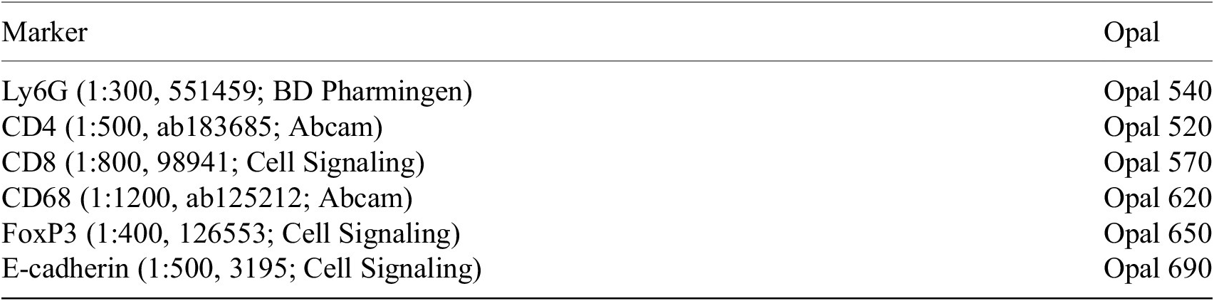
thickness. The staining was performed on the Leica BOND RXm auto-stainer (Leica Microsystems, Germany). Six consecutive staining cycles were conducted using primary antibody-Opal fluorophore pairs. The marker panel used is shown in Table 1.
$ \mu \mathrm{m} $
thickness. The staining was performed on the Leica BOND RXm auto-stainer (Leica Microsystems, Germany). Six consecutive staining cycles were conducted using primary antibody-Opal fluorophore pairs. The marker panel used is shown in Table 1.
List of markers and opals used in the multiplex panel
The tissue sections were incubated with primary antibody for an hour, and the BOND Polymer Refine Detection System (DS9800, Leica Biosystems, Buffalo Grove, IL) used to detect the antibodies. Epitope Retrieval Solution 1 or 2 was applied to retrieve the antigen for 20 min at 100 °C, in accordance with the standard Leica protocol, and, thereafter, each primary antibody was applied. The tissue sections were subsequently treated with spectral DAPI (FP1490, Akoya Biosciences) for 10 min and mounted with VECTASHIELD Vibrance Antifade Mounting Medium (H-1700-10; Vector Laboratories) slides. The Vectra Polaris (Akoya Biosciences) was used to obtain whole-slide scans and multispectral images (MSIs). Batch analysis of the MSIs from each case was performed using inForm 2.4.8 software, and the resultant batch-analyzed MSIs were combined in HALO (Indica Labs) to create a spectrally unmixed reconstructed whole-tissue image. Cell segmentation and phenotypic density analysis was conducted thereafter across the tissue using HALO.
2.2. ROI overview
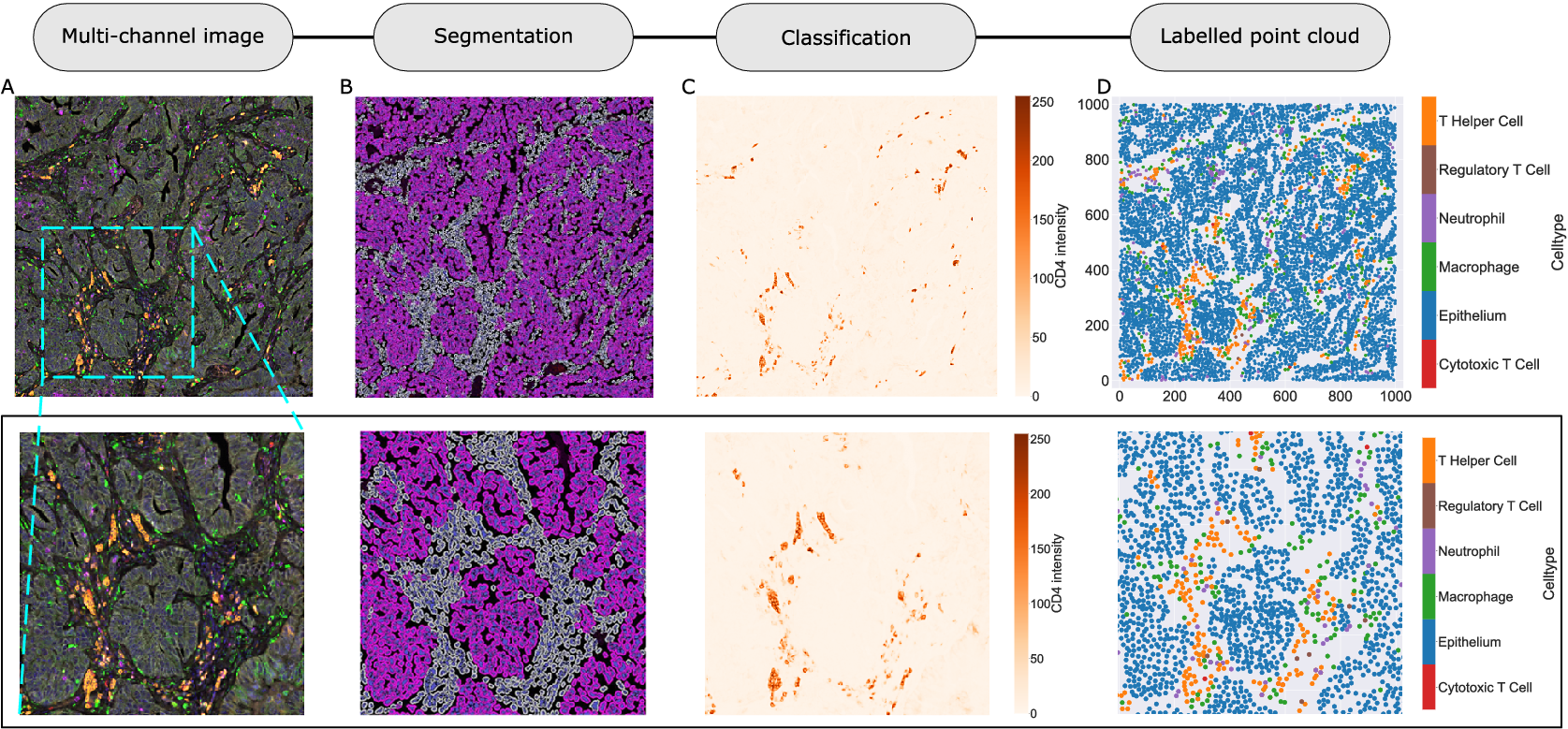
We consider a 1 mm × 1 mm ROI from a KPN mouse intestinal tumor, shown in Figure 1a (three additional regions from this tumor are included in the Supplementary Material). Each color channel corresponds to a different marker (blue – DAPI; orange – CD4; green – CD68; magenta – Ly6G; maroon – FoxP3; red – CD8; white – E-cadherin). To obtain a labeled point cloud, individual cell boundaries were identified via cell segmentation (HALO, panel b). Classification of cell types was achieved by considering the average pixel intensity within a cell boundary for each marker individually (e.g., CD4 pixel intensity, panel c), with combinations of cell markers defining different cell types as outlined in Table 2. The final marked point pattern (panel d) was obtained by assigning cell labels to the centroids associated with each cell boundary.
Obtaining point cloud data from a multiplex image. (a) 1 mm × 1 mm ROI from a multiplex IHC image of murine colorectal carcinoma (blue – DAPI; orange – CD4; green – CD68; magenta – Ly6G; maroon – FoxP3; red – CD8; white – E-cadherin). The epithelial cells (E-cadherin+) are cancer cells which form dense “tumor nests” that are surrounded by stromal regions. Immune cells are largely restricted to the stroma between tumor nests, so the region shows spatial correlation between immune cell subtypes (particularly macrophage, neutrophil, and T helper cell) within the stroma, and anticorrelation between immune cells and epithelial cells. (b) Cell segmentation (HALO) for the region in panel a. The edges of E-cadherin positive cells are shown in pink to aid comparison with panel a. (c) Pixel intensity from the color channel corresponding to the CD4 stain only. (d) Composite point cloud formed by classifying each cell type stained in panel a, with points placed at the centroids of segmented cells. Lower row: Magnified $ 500\hskip0.4em \mu \mathrm{m}\times 500\hskip0.4em \mu \mathrm{m} $
zoom from the upper panels.
$ 500\hskip0.4em \mu \mathrm{m}\times 500\hskip0.4em \mu \mathrm{m} $
zoom from the upper panels.
Cell types present in the ROI, with markers and number of cells present. Note that all cells must also contain sufficient DAPI staining to be classified as a cell. Due to low numbers of cytotoxic T cells and regulatory T cells, we exclude them from subsequent analyses
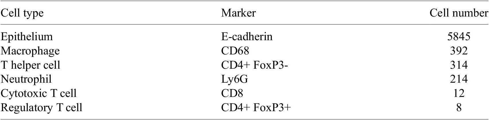
The ROI in Figure 1 was selected because of the clear separation between the spatial position of immune cell subtypes and tumor nests (epithelial cells), with immune cells located predominantly in regions between epithelial cell islands. Table 2 summarizes the different cell types, the markers used to define them, and the number of cells of each type in the ROI.
2.3. Spatial statistics
We consider a point pattern in a rectangular domain $ \Omega =\left[0,1000\hskip0.4em \mu \mathrm{m}\right]\times \left[0,1000\hskip0.4em \mu \mathrm{m}\right] $
. The point pattern comprises
$ \Omega =\left[0,1000\hskip0.4em \mu \mathrm{m}\right]\times \left[0,1000\hskip0.4em \mu \mathrm{m}\right] $
. The point pattern comprises $ N $
points (or cells). Cell
$ N $
points (or cells). Cell $ i $
(
$ i $
( $ i\in 1,2,\dots, N $
) has spatial location
$ i\in 1,2,\dots, N $
) has spatial location $ {\mathbf{x}}_{\mathbf{i}}=\left({x}_i,{y}_i\right) $
, and a set of marks which may be categorical (e.g., a label for a cell type, or a true/false label indicating whether a cell’s average stain intensity exceeds a threshold value), or continuous (e.g., the average stain intensity of a particular mark within a cell). For clarity, we denote categorical and continuous marks by
$ {\mathbf{x}}_{\mathbf{i}}=\left({x}_i,{y}_i\right) $
, and a set of marks which may be categorical (e.g., a label for a cell type, or a true/false label indicating whether a cell’s average stain intensity exceeds a threshold value), or continuous (e.g., the average stain intensity of a particular mark within a cell). For clarity, we denote categorical and continuous marks by $ c $
and
$ c $
and $ m $
, respectively. We use lowercase for marks associated with a particular point and uppercase for target values. We introduce the indicator function
$ m $
, respectively. We use lowercase for marks associated with a particular point and uppercase for target values. We introduce the indicator function $ \unicode{x1D540}\left(C,c\right) $
to determine whether a categorical mark associated with a point matches a target mark:
$ \unicode{x1D540}\left(C,c\right) $
to determine whether a categorical mark associated with a point matches a target mark:
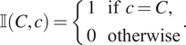 $$ \unicode{x1D540}\left(C,c\right)=\left\{\begin{array}{l}1\hskip1em \mathrm{if}\hskip0.4em c=C,\\ {}0\hskip1em \mathrm{otherwise}\end{array}\right.. $$
When we define correlation functions below, we will need to determine whether two points are separated by a distance “close to” $ r $
. We do this by defining an indicator function,
$ r $
. We do this by defining an indicator function, $ {I}_{\left[a,b\right)}(r) $
, which identifies whether the distance
$ {I}_{\left[a,b\right)}(r) $
, which identifies whether the distance $ r $
is within an interval
$ r $
is within an interval $ \left[a,b\right) $
:
$ \left[a,b\right) $
:
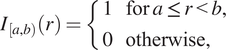 $$ {I}_{\left[a,b\right)}(r)=\left\{\begin{array}{ll}1& \mathrm{for}\hskip0.24em a\le r<b,\\ {}0& \mathrm{otherwise},\end{array}\right. $$
where $ a $
and
$ a $
and $ b $
are the real numbers with
$ b $
are the real numbers with $ a<b $
. We calculate the statistics below at a series of discrete points
$ a<b $
. We calculate the statistics below at a series of discrete points $ {r}_k $
, which is equivalent to considering a sequence of annuli of width
$ {r}_k $
, which is equivalent to considering a sequence of annuli of width $ dr>0 $
whose inner radii are separated by
$ dr>0 $
whose inner radii are separated by $ \delta r>0 $
, with
$ \delta r>0 $
, with $ {r}_{k+1}={r}_k+\delta r $
and
$ {r}_{k+1}={r}_k+\delta r $
and $ {r}_0=0 $
(if
$ {r}_0=0 $
(if $ dr=\delta r $
then the annuli are nonoverlapping). We denote by
$ dr=\delta r $
then the annuli are nonoverlapping). We denote by $ {A}_r\left(\mathbf{x}\right) $
the area of the annulus with inner radius
$ {A}_r\left(\mathbf{x}\right) $
the area of the annulus with inner radius $ r $
and width
$ r $
and width $ dr $
centered at the point
$ dr $
centered at the point $ \mathbf{x} $
, intersected with the domain. If this annulus lies wholly inside the domain then
$ \mathbf{x} $
, intersected with the domain. If this annulus lies wholly inside the domain then $ {A}_r\left(\mathbf{x}\right)=\pi \left({\left(r+ dr\right)}^2-{r}^2\right)=\pi \left(2r+ dr\right) dr $
; otherwise, only the area contained within the domain is recorded.
$ {A}_r\left(\mathbf{x}\right)=\pi \left({\left(r+ dr\right)}^2-{r}^2\right)=\pi \left(2r+ dr\right) dr $
; otherwise, only the area contained within the domain is recorded.
It is important to distinguish between the theoretical forms of correlation functions, which relate to properties of a point process which has generated a pattern, and the empirical forms of the same functions, which relate to observations of data (regardless of whether that data are generated from an underlying point process). In the definitions below, we consider only empirical versions of these functions, which may be defined differently (e.g., by using different kernels or edge-correction terms): for a detailed discussion of the differences between empirical and theoretical spatial statistics, we refer the interested reader to textbooks such as Reference (Reference Baddeley, Rubak and Turner45).
It is important to note that these functions cannot distinguish, in a technical sense, between colocalization of cells due to co-intensity (points being found in the same region due to, e.g., the tissue being partitioned into tumor and stromal regions) or correlation (points being found in the same region because they are subject to the same reference process). Since cell location data are not generated by a well-defined statistical process, statistical correlation and co-intensity cannot be readily distinguished using multiplex imaging data, and we use the terms interchangeably throughout this manuscript. We note also that, in this manuscript, we use statistics to illustrate their potential as tools to guide quantitative analysis of multiplex imaging. In order to assess the significance of these (or other) spatial statistics, appropriate significance testing should be performed. For a given statistic, this could be achieved by, for example, generating a simulation envelope using data derived from CSR and comparing this with the observed measurements.
2.3.1. Pair correlation function
2.3.1.1. Aims
The PCF, $ {g}_C(r) $
, quantifies spatial clustering or exclusion between pairs of points separated by a distance
$ {g}_C(r) $
, quantifies spatial clustering or exclusion between pairs of points separated by a distance $ r $
within an ROI, compared to a suitably selected null distribution. While a range of null distributions could be considered (e.g., using a Matérn hard core process to simulate randomly distributed cell centers separated by a minimum distance to approximate a cell radius(Reference Matérn
57
)), we assume the null distribution is complete spatial randomness (CSR) as represented by a homogeneous spatial Poisson point process with intensity
$ r $
within an ROI, compared to a suitably selected null distribution. While a range of null distributions could be considered (e.g., using a Matérn hard core process to simulate randomly distributed cell centers separated by a minimum distance to approximate a cell radius(Reference Matérn
57
)), we assume the null distribution is complete spatial randomness (CSR) as represented by a homogeneous spatial Poisson point process with intensity $ \lambda >0 $
chosen to match the intensity of the point pattern being analyzed.
$ \lambda >0 $
chosen to match the intensity of the point pattern being analyzed.
2.3.1.2. Definition
Let $ {N}_C={\sum}_{i=1}^N\unicode{x1D540}\left(C,{c}_i\right) $
be the number of points in
$ {N}_C={\sum}_{i=1}^N\unicode{x1D540}\left(C,{c}_i\right) $
be the number of points in $ \Omega $
with
$ \Omega $
with $ {c}_i=C $
, for some categorical mark
$ {c}_i=C $
, for some categorical mark $ C $
. The empirical PCF,
$ C $
. The empirical PCF, $ {g}_C(r) $
, is defined as follows:
$ {g}_C(r) $
, is defined as follows:
 $$ {g}_C(r)=\frac{1}{N_C}\sum \limits_{i=1}^N\unicode{x1D540}\left(C,{c}_i\right)\left(\sum \limits_{j=1}^N\unicode{x1D540}\left(C,{c}_j\right)\frac{I_{\left[0, dr\right)}\left(|{\mathbf{x}}_i-{\mathbf{x}}_j|-r\right)}{A_r\left({\mathbf{x}}_i\right)}/\frac{N_C}{A}\right) $$
where $ A $
is the total area of the domain
$ A $
is the total area of the domain $ \Omega $
and
$ \Omega $
and $ dr>0 $
. There are many ways to account for edge effects associated with points close to the domain boundary, although the choice of a particular method is generally not critical (see, e.g., Reference (Reference Baddeley, Rubak and Turner45) for a detailed discussion of this). Throughout this paper, we account for them by adjusting the contribution of each point to account for the area of each annulus contained within the domain,
$ dr>0 $
. There are many ways to account for edge effects associated with points close to the domain boundary, although the choice of a particular method is generally not critical (see, e.g., Reference (Reference Baddeley, Rubak and Turner45) for a detailed discussion of this). Throughout this paper, we account for them by adjusting the contribution of each point to account for the area of each annulus contained within the domain, $ {A}_r\left(\mathbf{x}\right) $
. This form of edge correction ensures that the local contribution to the PCF of a given point is based on the ratio of the observed number of points to the area of the annulus that falls within the domain; note that many other forms of edge correction are used throughout the literature,(Reference Baddeley, Rubak and Turner
45
) and can be substituted here without substantially changing the methods introduced below.
$ {A}_r\left(\mathbf{x}\right) $
. This form of edge correction ensures that the local contribution to the PCF of a given point is based on the ratio of the observed number of points to the area of the annulus that falls within the domain; note that many other forms of edge correction are used throughout the literature,(Reference Baddeley, Rubak and Turner
45
) and can be substituted here without substantially changing the methods introduced below.
For a theoretical PCF, CSR generates a value of 1. We note from Equation (3) that, for the empirical PCF, $ {g}_C(r)\approx 1 $
for data generated under CSR. Further, if
$ {g}_C(r)\approx 1 $
for data generated under CSR. Further, if $ {g}_C(r)>1 $
then points separated by distance
$ {g}_C(r)>1 $
then points separated by distance $ r $
are observed more frequently than expected under CSR and we say that points at this length scale are clustered relative to CSR. Similarly,
$ r $
are observed more frequently than expected under CSR and we say that points at this length scale are clustered relative to CSR. Similarly, $ {g}_C(r)<1 $
indicates fewer points than expected and is interpreted as exclusion at length scale
$ {g}_C(r)<1 $
indicates fewer points than expected and is interpreted as exclusion at length scale $ r $
.
$ r $
.
The structure of Equation (3) provides the basis for the generalizations of the PCF introduced below.
2.3.2. Cross PCF
2.3.2.1. Aims
The cross-PCF describes the correlation between pairs of points separated by distance $ r $
which may have different categorical labels.(Reference Baddeley, Rubak and Turner
45
)
$ r $
which may have different categorical labels.(Reference Baddeley, Rubak and Turner
45
)
2.3.2.2. Definition
Consider the categorical marks $ {C}_1 $
and
$ {C}_1 $
and $ {C}_2 $
. The cross-PCF,
$ {C}_2 $
. The cross-PCF, $ {g}_{C_1{C}_2}(r) $
, is defined as follows:
$ {g}_{C_1{C}_2}(r) $
, is defined as follows:
 $$ {g}_{C_1{C}_2}(r)=\frac{1}{N_{C_1}}\sum \limits_{i=1}^N\unicode{x1D540}\left({C}_1,{c}_i\right)\left(\sum \limits_{j=1}^N\unicode{x1D540}\left({C}_2,{c}_j\right)\frac{I_{\left[0, dr\right)}\left(|{\mathbf{x}}_i-{\mathbf{x}}_j|-r\right)}{A_r\left({\mathbf{x}}_i\right)}/\frac{N_{C_2}}{A}\right), $$
where $ {N}_{C_i}={\sum}_{j=1}^N\unicode{x1D540}\left({C}_i,{c}_j\right) $
is the number of points with mark
$ {N}_{C_i}={\sum}_{j=1}^N\unicode{x1D540}\left({C}_i,{c}_j\right) $
is the number of points with mark $ {C}_i $
. We note that when
$ {C}_i $
. We note that when $ {C}_1={C}_2 $
, Equation (4) reduces to Equation (3) (i.e., the cross-PCF reduces to the PCF).
$ {C}_1={C}_2 $
, Equation (4) reduces to Equation (3) (i.e., the cross-PCF reduces to the PCF).
2.3.2.3. Example
The interpretation of the cross-PCF is similar to that for the PCF, with $ {g}_{C_1{C}_2}(r)>1 $
indicating correlation between points with marks
$ {g}_{C_1{C}_2}(r)>1 $
indicating correlation between points with marks $ {C}_1 $
and
$ {C}_1 $
and $ {C}_2 $
separated by distance
$ {C}_2 $
separated by distance $ r $
and
$ r $
and $ {g}_{C_1{C}_2}(r)<1 $
indicating exclusion at distance
$ {g}_{C_1{C}_2}(r)<1 $
indicating exclusion at distance $ r $
.
$ r $
.
In Figure 2, we compute two cross-PCFs for synthetic dataset I. In Figure 2a, cells with labels $ {C}_1 $
and
$ {C}_1 $
and $ {C}_2 $
are strongly spatially correlated on the left half of the domain, while they are clustered separately on the right half. Figure 2b shows the cross-PCFs
$ {C}_2 $
are strongly spatially correlated on the left half of the domain, while they are clustered separately on the right half. Figure 2b shows the cross-PCFs $ {g}_{C_1{C}_2}(r) $
and
$ {g}_{C_1{C}_2}(r) $
and $ {g}_{C_2{C}_1}(r) $
for this point pattern. Colocalization between the cell types is identified for
$ {g}_{C_2{C}_1}(r) $
for this point pattern. Colocalization between the cell types is identified for $ r\hskip0.35em \lesssim \hskip0.35em 200 $
. The cross-PCFs are almost identical, since the cross-PCF is symmetric up to boundary correction terms. While the cross-PCF successfully identifies the presence of clustering between the two cell types, it does not provide information about differences in colocalization on the left- and right-hand sides of the domain.
$ r\hskip0.35em \lesssim \hskip0.35em 200 $
. The cross-PCFs are almost identical, since the cross-PCF is symmetric up to boundary correction terms. While the cross-PCF successfully identifies the presence of clustering between the two cell types, it does not provide information about differences in colocalization on the left- and right-hand sides of the domain.
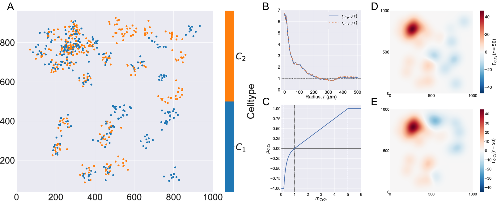
Motivating example I: Cross-PCF and topographical correlation map. (a) Synthetic dataset I: a synthetic point pattern involving two cell types, with labels $ {C}_1 $
and
$ {C}_1 $
and $ {C}_2 $
. For
$ {C}_2 $
. For $ 0\le x\le 500 $
, points with labels
$ 0\le x\le 500 $
, points with labels $ {C}_1 $
and
$ {C}_1 $
and $ {C}_2 $
cluster together; for
$ {C}_2 $
cluster together; for $ 500<x\le 1000 $
, points of types
$ 500<x\le 1000 $
, points of types $ {C}_1 $
and
$ {C}_1 $
and $ {C}_2 $
form distinct, homogeneous clusters. (b) The cross-PCFs
$ {C}_2 $
form distinct, homogeneous clusters. (b) The cross-PCFs $ {g}_{C_1{C}_2}(r) $
and
$ {g}_{C_1{C}_2}(r) $
and $ {g}_{C_2{C}_1}(r) $
for the point pattern in panel a. The cross-PCF detects the short range clustering between cells of types
$ {g}_{C_2{C}_1}(r) $
for the point pattern in panel a. The cross-PCF detects the short range clustering between cells of types $ {C}_1 $
and
$ {C}_1 $
and $ {C}_2 $
, which is present for
$ {C}_2 $
, which is present for $ 0\le x\le 500 $
. The cross-PCFs are almost identical, differing only for large
$ 0\le x\le 500 $
. The cross-PCFs are almost identical, differing only for large $ r $
because of boundary correction terms. (c) Function used to linearize the mark
$ r $
because of boundary correction terms. (c) Function used to linearize the mark $ {m}_{C_1{C}_2} $
in Equation (6), used to calculate the TCM, for
$ {m}_{C_1{C}_2} $
in Equation (6), used to calculate the TCM, for $ \alpha =5 $
. Dashed lines represent
$ \alpha =5 $
. Dashed lines represent $ {m}_{C_1{C}_2}=1/\alpha, 1,\alpha $
, which correspond to the maximum detectable exclusion, CSR, and the maximum detectable clustering. (d, e) TCMs
$ {m}_{C_1{C}_2}=1/\alpha, 1,\alpha $
, which correspond to the maximum detectable exclusion, CSR, and the maximum detectable clustering. (d, e) TCMs $ {\Gamma}_{C_1{C}_2}\left(r=50,\mathbf{x}\right) $
and
$ {\Gamma}_{C_1{C}_2}\left(r=50,\mathbf{x}\right) $
and $ {\Gamma}_{C_2{C}_1}\left(r=50,\mathbf{x}\right) $
. The TCM identifies colocalization between cells of types
$ {\Gamma}_{C_2{C}_1}\left(r=50,\mathbf{x}\right) $
. The TCM identifies colocalization between cells of types $ {C}_1 $
and
$ {C}_1 $
and $ {C}_2 $
in
$ {C}_2 $
in $ 0\le x\le 500 $
, and distinguishes between the dense cluster in the top left quadrant and smaller clusters in the bottom left quadrant. The TCM also identifies exclusion between the two cell populations in
$ 0\le x\le 500 $
, and distinguishes between the dense cluster in the top left quadrant and smaller clusters in the bottom left quadrant. The TCM also identifies exclusion between the two cell populations in $ 500\le x\le 1000 $
and shows this to be less pronounced than the clustering in
$ 500\le x\le 1000 $
and shows this to be less pronounced than the clustering in $ 0\le x\le 500 $
. Note that while the regions of positive correlation are similar between panels d and e, the regions of negative correlation differ.
$ 0\le x\le 500 $
. Note that while the regions of positive correlation are similar between panels d and e, the regions of negative correlation differ.
2.3.3. Topographical correlation map
2.3.3.1. Aims
The TCM, $ {\Gamma}_{C_1{C}_2}\left(r,\mathbf{x}\right) $
, is an example of a LISA(Reference Anselin
50
) and was introduced by us in Reference (Reference Weeratunga, Denney and Bull7) to visualize spatial heterogeneity in the correlation between pairs of points across an ROI. In contrast to direct visualization of two point patterns, the TCM provides a quantitative summary of colocalization between the points which is spatially resolved across the ROI. Local maxima and minima of the TCM identify areas where points with different labels are (positively or negatively) correlated, relative to a baseline of CSR. Motivated by Equation (4), each point with mark
$ {\Gamma}_{C_1{C}_2}\left(r,\mathbf{x}\right) $
, is an example of a LISA(Reference Anselin
50
) and was introduced by us in Reference (Reference Weeratunga, Denney and Bull7) to visualize spatial heterogeneity in the correlation between pairs of points across an ROI. In contrast to direct visualization of two point patterns, the TCM provides a quantitative summary of colocalization between the points which is spatially resolved across the ROI. Local maxima and minima of the TCM identify areas where points with different labels are (positively or negatively) correlated, relative to a baseline of CSR. Motivated by Equation (4), each point with mark $ {C}_1 $
is assigned a value that quantifies its correlation with points with mark
$ {C}_1 $
is assigned a value that quantifies its correlation with points with mark $ {C}_2 $
. A series of kernels centered at each point with mark
$ {C}_2 $
. A series of kernels centered at each point with mark $ {C}_1 $
is summed to produce a spatial map of local correlations between the cell types. We note that, since these kernels are centered on points marked
$ {C}_1 $
is summed to produce a spatial map of local correlations between the cell types. We note that, since these kernels are centered on points marked $ {C}_1 $
, the TCM is not symmetric (i.e.,
$ {C}_1 $
, the TCM is not symmetric (i.e., $ {\Gamma}_{C_1{C}_2}\ne {\Gamma}_{C_2{C}_1} $
if
$ {\Gamma}_{C_1{C}_2}\ne {\Gamma}_{C_2{C}_1} $
if $ {C}_1\ne {C}_2 $
).
$ {C}_1\ne {C}_2 $
).
2.3.3.2. Definition
The TCM, $ {\Gamma}_{C_1{C}_2}\left(r,\mathbf{x}\right) $
, is visualized at a specific length scale
$ {\Gamma}_{C_1{C}_2}\left(r,\mathbf{x}\right) $
, is visualized at a specific length scale $ r $
, chosen to reflect the length scale at which one wishes to observe correlation. The choice of length scale can be determined from the corresponding cross-PCF
$ r $
, chosen to reflect the length scale at which one wishes to observe correlation. The choice of length scale can be determined from the corresponding cross-PCF $ {g}_{C_1,{C}_2}(r) $
, by identifying the value at which
$ {g}_{C_1,{C}_2}(r) $
, by identifying the value at which $ g(r)\approx 1 $
, for example, or based on a priori assumptions about biological behavior, for example by choosing a length scale associated with the approximate size of the cells of interest. Unless stated otherwise, we fix
$ g(r)\approx 1 $
, for example, or based on a priori assumptions about biological behavior, for example by choosing a length scale associated with the approximate size of the cells of interest. Unless stated otherwise, we fix $ r=50\mu \mathrm{m} $
which corresponds to clustering on the length scale of two to three cell diameters. We associate a continuous mark
$ r=50\mu \mathrm{m} $
which corresponds to clustering on the length scale of two to three cell diameters. We associate a continuous mark $ {m}_{C_1{C}_2}\left(r,{\mathbf{x}}_i\right) $
with each cell
$ {m}_{C_1{C}_2}\left(r,{\mathbf{x}}_i\right) $
with each cell $ i $
with mark
$ i $
with mark $ {C}_1 $
, such that
$ {C}_1 $
, such that
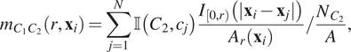 $$ {m}_{C_1{C}_2}\left(r,{\mathbf{x}}_i\right)=\sum \limits_{j=1}^N\unicode{x1D540}\left({C}_2,{c}_j\right)\frac{I_{\left[0,r\right)}\left(|{\mathbf{x}}_i-{\mathbf{x}}_j|\right)}{A_r\left({\mathbf{x}}_i\right)}/\frac{N_{C_2}}{A}, $$
where $ {A}_r\left({\mathbf{x}}_i\right) $
is the area of that part of the circle with radius
$ {A}_r\left({\mathbf{x}}_i\right) $
is the area of that part of the circle with radius $ r\mu \mathrm{m} $
centered at
$ r\mu \mathrm{m} $
centered at $ {\mathbf{x}}_i $
that falls within the ROI.
$ {\mathbf{x}}_i $
that falls within the ROI. $ {m}_{C_1{C}_2}\left(r,{\mathbf{x}}_i\right) $
can be viewed as the contribution of each point
$ {m}_{C_1{C}_2}\left(r,{\mathbf{x}}_i\right) $
can be viewed as the contribution of each point $ i $
to the cross-PCF,
$ i $
to the cross-PCF, $ {g}_{C_1{C}_2}(r) $
, for the special case of an annulus with inner radius 0 and width
$ {g}_{C_1{C}_2}(r) $
, for the special case of an annulus with inner radius 0 and width $ dr=r $
(note that this represents the cumulative contributions of the annuli used to calculate the cross-PCF up to distance
$ dr=r $
(note that this represents the cumulative contributions of the annuli used to calculate the cross-PCF up to distance $ r $
; that is, the contribution to the K-function – see, e.g., Reference (Reference Baddeley, Rubak and Turner45)). Thus,
$ r $
; that is, the contribution to the K-function – see, e.g., Reference (Reference Baddeley, Rubak and Turner45)). Thus, $ {m}_{C_1{C}_2}\left(r,{\mathbf{x}}_i\right) $
is interpreted similarly to the cross-PCF:
$ {m}_{C_1{C}_2}\left(r,{\mathbf{x}}_i\right) $
is interpreted similarly to the cross-PCF: $ {m}_{C_1{C}_2}\left(r,{\mathbf{x}}_i\right)<1 $
indicates anticorrelation between cells with marks
$ {m}_{C_1{C}_2}\left(r,{\mathbf{x}}_i\right)<1 $
indicates anticorrelation between cells with marks $ {C}_1 $
and
$ {C}_1 $
and $ {C}_2 $
separated by a distance of at most
$ {C}_2 $
separated by a distance of at most $ r\mu \mathrm{m} $
, and
$ r\mu \mathrm{m} $
, and $ {m}_{C_1{C}_2}\left(r,{\mathbf{x}}_i\right)>1 $
indicates correlation.
$ {m}_{C_1{C}_2}\left(r,{\mathbf{x}}_i\right)>1 $
indicates correlation.
Since $ {m}_{C_1{C}_2}\left(r,{\mathbf{x}}_i\right) $
is based on a ratio of observed counts to counts expected under CSR, its interpretation is nonlinear: an observation of three times as many points as expected corresponds to
$ {m}_{C_1{C}_2}\left(r,{\mathbf{x}}_i\right) $
is based on a ratio of observed counts to counts expected under CSR, its interpretation is nonlinear: an observation of three times as many points as expected corresponds to $ {m}_{C_1{C}_2}\left(r,{\mathbf{x}}_i\right)=3 $
, while three times fewer points than expected leads to
$ {m}_{C_1{C}_2}\left(r,{\mathbf{x}}_i\right)=3 $
, while three times fewer points than expected leads to $ {m}_{C_1{C}_2}\left(r,{\mathbf{x}}_i\right)=1/3 $
. To facilitate interpretation, we rescale
$ {m}_{C_1{C}_2}\left(r,{\mathbf{x}}_i\right)=1/3 $
. To facilitate interpretation, we rescale $ {m}_{C_1{C}_2}\left(r,{\mathbf{x}}_i\right) $
to produce a transformed mark
$ {m}_{C_1{C}_2}\left(r,{\mathbf{x}}_i\right) $
to produce a transformed mark $ {\mu}_{C_1{C}_2}\left(r,{\mathbf{x}}_i\right) $
in which clustering and exclusion can be compared on a linear scale, with
$ {\mu}_{C_1{C}_2}\left(r,{\mathbf{x}}_i\right) $
in which clustering and exclusion can be compared on a linear scale, with $ {\mu}_{C_1{C}_2}\left(r,{\mathbf{x}}_i\right)=0 $
when
$ {\mu}_{C_1{C}_2}\left(r,{\mathbf{x}}_i\right)=0 $
when $ {m}_{C_1{C}_2}\left(r,{\mathbf{x}}_i\right)=1 $
:
$ {m}_{C_1{C}_2}\left(r,{\mathbf{x}}_i\right)=1 $
:
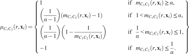 $$ {\mu}_{C_1{C}_2}\left(r,{\mathbf{x}}_i\right)=\left\{\begin{array}{lll}1& \hskip3em \mathrm{if}& {m}_{C_1{C}_2}\left(r,{\mathbf{x}}_i\right)\ge \alpha, \\ {}\left(\frac{1}{\alpha -1}\right)\left({m}_{C_1{C}_2}\left(r,{\mathbf{x}}_i\right)-1\right)\hskip3em & \hskip3em \mathrm{if}& 1<{m}_{C_1{C}_2}\left(r,{\mathbf{x}}_i\right)\le \alpha, \\ {}\left(\frac{1}{\alpha -1}\right)\left(1-\frac{1}{m_{C_1{C}_2}\left(r,{\mathbf{x}}_i\right)}\right)& \hskip3em \mathrm{if}& \frac{1}{\alpha }<{m}_{C_1{C}_2}\left(r,{\mathbf{x}}_i\right)\le 1,\\ {}-1& \hskip3em \mathrm{if}& {m}_{C_1{C}_2}\left(r,{\mathbf{x}}_i\right)\le \frac{1}{\alpha }.\end{array}\right\} $$
In Equation (6), the constant $ \alpha \hskip0.2em >1 $
describes the maximal degree of clustering (or exclusion) which can be resolved under this transformation. A sketch of Equation (6) is presented in Figure 2c, for
$ \alpha \hskip0.2em >1 $
describes the maximal degree of clustering (or exclusion) which can be resolved under this transformation. A sketch of Equation (6) is presented in Figure 2c, for $ \alpha =5 $
(henceforth, we fix
$ \alpha =5 $
(henceforth, we fix $ \alpha =5 $
).
$ \alpha =5 $
).
After calculating $ {\mu}_{C_1{C}_2}\left(r,{\mathbf{x}}_i\right) $
for each cell with mark
$ {\mu}_{C_1{C}_2}\left(r,{\mathbf{x}}_i\right) $
for each cell with mark $ {C}_1 $
, we center a Gaussian kernel with standard deviation
$ {C}_1 $
, we center a Gaussian kernel with standard deviation $ \sigma = r\mu \mathrm{m} $
, and scaled by
$ \sigma = r\mu \mathrm{m} $
, and scaled by $ {\mu}_{C_1{C}_2} $
, at
$ {\mu}_{C_1{C}_2} $
, at $ {\mathbf{x}}_i $
(examples showing the effect of varying
$ {\mathbf{x}}_i $
(examples showing the effect of varying $ r $
and
$ r $
and $ \sigma $
on the TCM are presented in the Supplementary Material). The TCM,
$ \sigma $
on the TCM are presented in the Supplementary Material). The TCM, $ {\Gamma}_{C_1{C}_2}\left(r,\mathbf{x}\right) $
, is obtained by summing over all cells with mark
$ {\Gamma}_{C_1{C}_2}\left(r,\mathbf{x}\right) $
, is obtained by summing over all cells with mark $ {C}_1 $
in the domain:
$ {C}_1 $
in the domain:
 $$ {\Gamma}_{C_1{C}_2}\left(r,\mathbf{x}\right)=\sum \limits_{i=1}^{N_{C_1}}\frac{\mu_{C_1{C}_2}}{2{\pi \sigma}^2}{e}^{-\frac{1}{2}{\left(\frac{\mid \mathbf{x}-{\mathbf{x}}_i\mid }{\sigma}\right)}^2}. $$
Regions in which the TCM is positive indicate that more points marked $ {C}_1 $
are positively correlated with points marked
$ {C}_1 $
are positively correlated with points marked $ {C}_2 $
in this area than would be expected under CSR, at length scales up to
$ {C}_2 $
in this area than would be expected under CSR, at length scales up to $ r\mu \mathrm{m} $
. Similarly, the TCM is negative in regions where points with mark
$ r\mu \mathrm{m} $
. Similarly, the TCM is negative in regions where points with mark $ {C}_1 $
are negatively correlated with points with mark
$ {C}_1 $
are negatively correlated with points with mark $ {C}_2 $
. The choice of
$ {C}_2 $
. The choice of $ \sigma $
changes the resolution of the TCM; we choose
$ \sigma $
changes the resolution of the TCM; we choose $ \sigma =r $
so that the resolution of the TCM approximately matches the maximum radius at which correlation contributes to the TCM (see the Supplementary Material for further details).
$ \sigma =r $
so that the resolution of the TCM approximately matches the maximum radius at which correlation contributes to the TCM (see the Supplementary Material for further details).
2.3.3.3. Example
Figure 2d,e shows the TCMs associated with synthetic dataset I (the point pattern in Figure 2a) for $ r=50 $
. Panel d shows
$ r=50 $
. Panel d shows $ {\Gamma}_{C_1{C}_2}\left(r=50,\mathbf{x}\right) $
and panel e shows
$ {\Gamma}_{C_1{C}_2}\left(r=50,\mathbf{x}\right) $
and panel e shows $ {\Gamma}_{C_2{C}_1}\left(r=50,\mathbf{x}\right) $
. Both TCMs identify differences in the colocalization of the two cell types on the left and right sides of the domain. In particular,
$ {\Gamma}_{C_2{C}_1}\left(r=50,\mathbf{x}\right) $
. Both TCMs identify differences in the colocalization of the two cell types on the left and right sides of the domain. In particular, $ {\Gamma}_{C_1{C}_2}\left(r=50,\mathbf{x}\right)\approx 40 $
in the upper left quadrant of panels d and e, indicating strong positive correlation, with weak association in the lower left (
$ {\Gamma}_{C_1{C}_2}\left(r=50,\mathbf{x}\right)\approx 40 $
in the upper left quadrant of panels d and e, indicating strong positive correlation, with weak association in the lower left ( $ {\Gamma}_{C_1{C}_2}\left(r=50,\mathbf{x}\right)\approx 10 $
). (Note that nonzero values of
$ {\Gamma}_{C_1{C}_2}\left(r=50,\mathbf{x}\right)\approx 10 $
). (Note that nonzero values of $ \Gamma $
are consistent with clustering or regularity. In practice, however, significance testing should be conducted before concluding that the observed value is significantly different from
$ \Gamma $
are consistent with clustering or regularity. In practice, however, significance testing should be conducted before concluding that the observed value is significantly different from $ \Gamma =0 $
.) For
$ \Gamma =0 $
.) For $ x\ge 500 $
both TCMs correctly identify the regions in which cells of types
$ x\ge 500 $
both TCMs correctly identify the regions in which cells of types $ {C}_1 $
and
$ {C}_1 $
and $ {C}_2 $
appear independently from one another (
$ {C}_2 $
appear independently from one another ( $ {\Gamma}_{C_1{C}_2}\left(r=50,\mathbf{x}\right)\approx -10 $
). The cross-PCFs in panel b are dominated by the correlation on the left-hand side of the domain, and are unable to resolve the heterogeneity in clustering between the left and right sides of the domain. We note that
$ {\Gamma}_{C_1{C}_2}\left(r=50,\mathbf{x}\right)\approx -10 $
). The cross-PCFs in panel b are dominated by the correlation on the left-hand side of the domain, and are unable to resolve the heterogeneity in clustering between the left and right sides of the domain. We note that $ {\Gamma}_{C_1{C}_2}\left(r,\mathbf{x}\right)\ne {\Gamma}_{C_2{C}_1}\left(r,\mathbf{x}\right) $
, since the kernels used to construct the TCM are centered on cells with label
$ {\Gamma}_{C_1{C}_2}\left(r,\mathbf{x}\right)\ne {\Gamma}_{C_2{C}_1}\left(r,\mathbf{x}\right) $
, since the kernels used to construct the TCM are centered on cells with label $ {C}_1 $
(and vice versa). While areas in which cells with mark
$ {C}_1 $
(and vice versa). While areas in which cells with mark $ {C}_1 $
and mark
$ {C}_1 $
and mark $ {C}_2 $
are co-located are identified by positive values of both
$ {C}_2 $
are co-located are identified by positive values of both $ {\Gamma}_{C_1{C}_2}\left(r,\mathbf{x}\right) $
and
$ {\Gamma}_{C_1{C}_2}\left(r,\mathbf{x}\right) $
and $ {\Gamma}_{C_2{C}_1}\left(r,\mathbf{x}\right) $
, their values differ in regions where one or other TCM is negative, as in these regions the cell densities vary (e.g., on the right-hand side of panels d and e). We, therefore, emphasize that
$ {\Gamma}_{C_2{C}_1}\left(r,\mathbf{x}\right) $
, their values differ in regions where one or other TCM is negative, as in these regions the cell densities vary (e.g., on the right-hand side of panels d and e). We, therefore, emphasize that $ {\Gamma}_{C_1{C}_2}\left(r,\mathbf{x}\right) $
provides a spatial map of subregions in which cells with mark
$ {\Gamma}_{C_1{C}_2}\left(r,\mathbf{x}\right) $
provides a spatial map of subregions in which cells with mark $ {C}_1 $
are correlated (or anticorrelated) with cells with mark
$ {C}_1 $
are correlated (or anticorrelated) with cells with mark $ {C}_2 $
. Finally, we note that the TCM is not a density map showing the presence (or absence) of the cell types individually; for example, when
$ {C}_2 $
. Finally, we note that the TCM is not a density map showing the presence (or absence) of the cell types individually; for example, when $ {\Gamma}_{C_1{C}_2}\left(r,\mathbf{x}\right)\approx 0 $
, either cells of type
$ {\Gamma}_{C_1{C}_2}\left(r,\mathbf{x}\right)\approx 0 $
, either cells of type $ {C}_1 $
are absent, or cells of both types are present in numbers consistent with CSR.
$ {C}_1 $
are absent, or cells of both types are present in numbers consistent with CSR.
2.3.4. Neighbourhood correlation function
2.3.4.1. Aims
The NCF $ (r) $
extends the PCF to quantify spatial colocation between three or more cell types with different categorical marks. We compare the observed number of triplets of points with marks
$ (r) $
extends the PCF to quantify spatial colocation between three or more cell types with different categorical marks. We compare the observed number of triplets of points with marks $ {C}_1,{C}_2 $
and
$ {C}_1,{C}_2 $
and $ {C}_3 $
within a neighbourhood of size
$ {C}_3 $
within a neighbourhood of size $ r $
against the number of triplets expected under CSR. Selecting an appropriate definition for such a neighbourhood is nontrivial: while it is straightforward to calculate the Euclidean distance between two points, many metrics can be used to calculate the proximity of three or more points. We require a metric that is interpretable and extends naturally to more than three points. Metrics such as the area of the polygon spanning the points are unsuitable (the area of the polygon is identically zero when all points fall on a straight line, even though the points could be far apart). We consider the minimum enclosing circle (details below) as it requires all cells to lie within a “neighbourhood” of each other (with the distance between any two points at most
$ r $
against the number of triplets expected under CSR. Selecting an appropriate definition for such a neighbourhood is nontrivial: while it is straightforward to calculate the Euclidean distance between two points, many metrics can be used to calculate the proximity of three or more points. We require a metric that is interpretable and extends naturally to more than three points. Metrics such as the area of the polygon spanning the points are unsuitable (the area of the polygon is identically zero when all points fall on a straight line, even though the points could be far apart). We consider the minimum enclosing circle (details below) as it requires all cells to lie within a “neighbourhood” of each other (with the distance between any two points at most $ 2r $
, where
$ 2r $
, where $ r $
is the radius of the minimum enclosing circle). While some methods instead consider the maximum pairwise distance between any two of the points to define the distance between a set of points (see, e.g., Reference (Reference Baddeley, Rubak and Turner45)), this is sensitive only to the location of the pair of points separated by the largest distance, and not to the location of other points in the set. The radius of the minimum enclosing circle can be interpreted in terms of pairwise distances (it is the length that minimizes the largest distance of any point from a common location, the center of the circle), but has a more natural interpretation in biological imaging contexts as the radius of the region in which the cells of interest are located.
$ r $
is the radius of the minimum enclosing circle). While some methods instead consider the maximum pairwise distance between any two of the points to define the distance between a set of points (see, e.g., Reference (Reference Baddeley, Rubak and Turner45)), this is sensitive only to the location of the pair of points separated by the largest distance, and not to the location of other points in the set. The radius of the minimum enclosing circle can be interpreted in terms of pairwise distances (it is the length that minimizes the largest distance of any point from a common location, the center of the circle), but has a more natural interpretation in biological imaging contexts as the radius of the region in which the cells of interest are located.
2.3.4.2. Definition
Consider a point pattern for which there are $ {N}_1 $
,
$ {N}_1 $
, $ {N}_2 $
, and
$ {N}_2 $
, and $ {N}_3 $
points with categorical marks
$ {N}_3 $
points with categorical marks $ {C}_1,{C}_2 $
, and
$ {C}_1,{C}_2 $
, and $ {C}_3 $
, respectively. We say that three points from this pattern fall within a “neighbourhood” of radius
$ {C}_3 $
, respectively. We say that three points from this pattern fall within a “neighbourhood” of radius $ r $
if there is a circle of radius
$ r $
if there is a circle of radius $ r $
which encloses all three points. For a given set of three points
$ r $
which encloses all three points. For a given set of three points $ \zeta =\left\{{\mathbf{x}}_1,{\mathbf{x}}_2,{\mathbf{x}}_3\right\} $
, let
$ \zeta =\left\{{\mathbf{x}}_1,{\mathbf{x}}_2,{\mathbf{x}}_3\right\} $
, let $ R\left(\zeta \right) $
be the radius of the smallest circle enclosing every point in
$ R\left(\zeta \right) $
be the radius of the smallest circle enclosing every point in $ \zeta $
(the “minimum enclosing circle”).
$ \zeta $
(the “minimum enclosing circle”).
There are $ {N}_1\times {N}_2\times {N}_3 $
possible triplets containing one point with each mark. We calculate
$ {N}_1\times {N}_2\times {N}_3 $
possible triplets containing one point with each mark. We calculate $ R $
for each of these, and then determine the number of circles of radius
$ R $
for each of these, and then determine the number of circles of radius $ r $
containing a unique grouping of cells with each mark (as for the PCF, these values are grouped into discrete bins of width
$ r $
containing a unique grouping of cells with each mark (as for the PCF, these values are grouped into discrete bins of width $ dr $
).
$ dr $
).
As for the PCF, we compare the number of minimum enclosing circles with radius $ r $
with the number expected under CSR. The probability of three points lying within a neighbourhood of radius
$ r $
with the number expected under CSR. The probability of three points lying within a neighbourhood of radius $ r $
,
$ r $
, $ {p}_3(r) $
, is:
$ {p}_3(r) $
, is:
 $$ {p}_3(r)=\underset{M\to \infty }{\lim}\frac{\sum_{i=1}^M{I}_{\left[0, dr\right)}\left(R\left(\left\{{\mathbf{x}}_i^1,{\mathbf{x}}_i^2,{\mathbf{x}}_i^3\right\}\right)-r\right)}{M}, $$
where $ {\mathbf{x}}_i^1 $
,
$ {\mathbf{x}}_i^1 $
, $ {\mathbf{x}}_i^2 $
, and
$ {\mathbf{x}}_i^2 $
, and $ {\mathbf{x}}_i^3 $
are three points within the domain, sampled under CSR. Since sampling such points is computationally cheap,
$ {\mathbf{x}}_i^3 $
are three points within the domain, sampled under CSR. Since sampling such points is computationally cheap, $ {p}_3(r) $
can practically be approximated for an arbitrary domain by sampling a large number of random triplets (in this section, we use
$ {p}_3(r) $
can practically be approximated for an arbitrary domain by sampling a large number of random triplets (in this section, we use $ M={10}^7 $
) and calculating their minimum enclosing circles. There are many standard algorithms for computing the radii of minimum enclosing circles (see, e.g., Reference (Reference Megiddo58), or (Reference Welzl and Maurer59) for the algorithm we use).
$ M={10}^7 $
) and calculating their minimum enclosing circles. There are many standard algorithms for computing the radii of minimum enclosing circles (see, e.g., Reference (Reference Megiddo58), or (Reference Welzl and Maurer59) for the algorithm we use).
For a point pattern containing $ N $
points, the NCF is defined as the ratio of the observed number of smallest neighbourhoods of radius
$ N $
points, the NCF is defined as the ratio of the observed number of smallest neighbourhoods of radius $ r $
to the number of such neighbourhoods expected under CSR,
$ r $
to the number of such neighbourhoods expected under CSR, $ {N}_1\times {N}_2\times {N}_3\times {p}_3(r) $
:
$ {N}_1\times {N}_2\times {N}_3\times {p}_3(r) $
:
 $$ {NCF}_{C_1{C}_2{C}_3}(r)=\sum \limits_{i=1}^N\sum \limits_{j=1}^N\sum \limits_{k=1}^N\unicode{x1D540}\left({C}_1,{c}_i\right)\unicode{x1D540}\left({C}_2,{c}_j\right)\unicode{x1D540}\left({C}_3,{c}_k\right)\frac{I_{\left[0, dr\right)}\left(R\left(\left\{{\mathbf{x}}_i,{\mathbf{x}}_j,{\mathbf{x}}_k\right\}\right)-r\right)}{\left({N}_1\times {N}_2\times {N}_3\right){p}_3(r).} $$
We note that it is straightforward to extend the NCF for $ n $
categorical marks:
$ n $
categorical marks:
 $$ {NCF}_{C_1\dots {C}_n}(r)=\sum \limits_{i_1=1}^N\dots \sum \limits_{i_n=1}^N\unicode{x1D540}\left({C}_{i_1},{c}_{i_1}\right)\times \dots \times \unicode{x1D540}\left({C}_{i_n},{c}_{i_n}\right)\frac{I_{\left[0, dr\right)}\left(R\left(\left\{{\mathbf{x}}_{i_1},\dots, {\mathbf{x}}_{i_n}\right\}\right)-r\right)}{\left({N}_1\times \dots \times {N}_n\right){p}_n(r)}, $$
where $ {p}_n(r) $
is the probability that
$ {p}_n(r) $
is the probability that $ n $
points sampled under CSR fall within a minimum enclosing circle of radius
$ n $
points sampled under CSR fall within a minimum enclosing circle of radius $ r $
.
$ r $
.
2.3.4.3. Example
As for the PCF, $ NCF(r)>1 $
indicates clustering and
$ NCF(r)>1 $
indicates clustering and $ NCF(r)<1 $
indicates exclusion. We interpret the length scale
$ NCF(r)<1 $
indicates exclusion. We interpret the length scale $ r $
associated with the NCF as the neighbourhood radius within which the points are contained.
$ r $
associated with the NCF as the neighbourhood radius within which the points are contained.
In Figure 3, we compare the cross-PCFs and $ {NCF}_{C_1{C}_2{C}_3} $
for the two point patterns from synthetic dataset II. In Figure 3a, each cluster consists of only two cell types, so that any pairwise combination of cell types can be found in close proximity while all three cell types are never in close proximity. In Figure 3e, each cluster contains all three cell types.
$ {NCF}_{C_1{C}_2{C}_3} $
for the two point patterns from synthetic dataset II. In Figure 3a, each cluster consists of only two cell types, so that any pairwise combination of cell types can be found in close proximity while all three cell types are never in close proximity. In Figure 3e, each cluster contains all three cell types.
Motivating example II: Neighbourhood Correlation Function. (a, e) Synthetic dataset II: point patterns in which three cell types are spatially correlated pairwise (a) or in triplets (e). In (a), each cluster contains only two cell types, so that all three cell types are never in close proximity. In (e), all three cell types are in close proximity in each cluster. Hence, in both point patterns, there is positive correlation between pairwise combinations of cell types, but the three-way correlations differ between the panels. (b, f) Cross-PCFs for the point patterns in panels a and e, respectively. These cross-PCFs appear identical, showing strong short-range correlation between the cell types (inside a cluster), exclusion from $ r=0.2 $
to
$ r=0.2 $
to $ r=0.4 $
, and a second peak of correlation around
$ r=0.4 $
, and a second peak of correlation around $ r=0.6 $
(between clusters). (c, g) Minimum enclosing circle for every combination of three points with marks
$ r=0.6 $
(between clusters). (c, g) Minimum enclosing circle for every combination of three points with marks $ {C}_1 $
,
$ {C}_1 $
, $ {C}_2 $
, and
$ {C}_2 $
, and $ {C}_3 $
(up to circles with a radius of
$ {C}_3 $
(up to circles with a radius of $ r=0.3 $
). Circles with small radii arise when all three cell types are in close proximity (panel g). Circles are colored according to their radius. (d, h) NCFs for the point patterns in panels a and e, respectively. The NCF in panel d correctly identifies short-range exclusion between the three cell types in panel a, while the NCF in panel h identifies strong short-range correlation between the three cell types.
$ r=0.3 $
). Circles with small radii arise when all three cell types are in close proximity (panel g). Circles are colored according to their radius. (d, h) NCFs for the point patterns in panels a and e, respectively. The NCF in panel d correctly identifies short-range exclusion between the three cell types in panel a, while the NCF in panel h identifies strong short-range correlation between the three cell types.
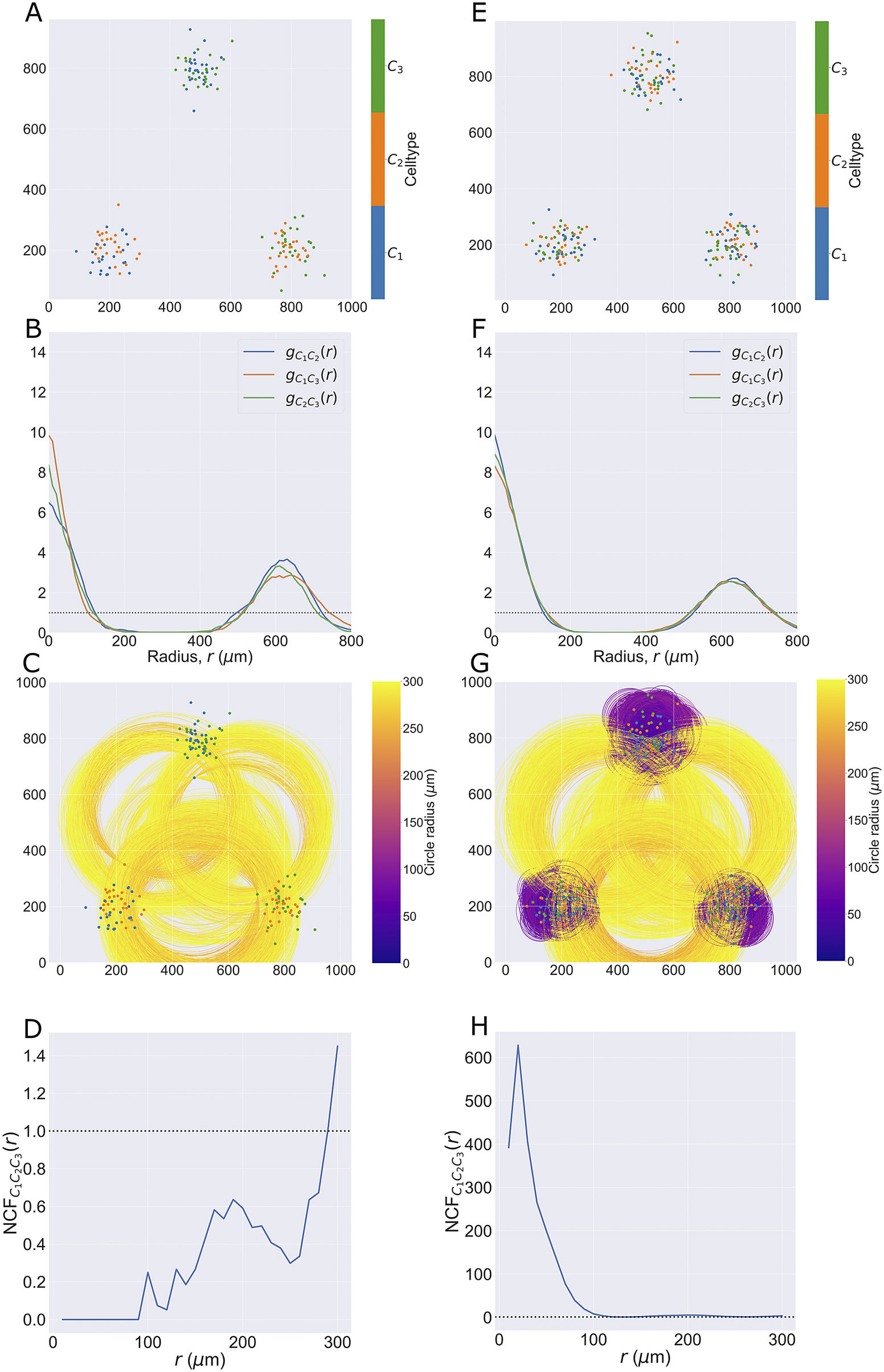
Figure 3b,f shows that, for synthetic dataset II, all cross-PCFs $ {g}_{C_1{C}_2} $
,
$ {g}_{C_1{C}_2} $
, $ {g}_{C_1{C}_3} $
, and
$ {g}_{C_1{C}_3} $
, and $ {g}_{C_2{C}_3} $
have the same shape and, hence, that pairwise correlation is insufficient to distinguish the two point patterns in this dataset. Figure 3c,g shows all minimum enclosing circles (with radius up to
$ {g}_{C_2{C}_3} $
have the same shape and, hence, that pairwise correlation is insufficient to distinguish the two point patterns in this dataset. Figure 3c,g shows all minimum enclosing circles (with radius up to $ 300\hskip0.4em \mu \mathrm{m} $
) for these point patterns, colored according to the radius of the circle; note that when all three cell types are present within the same cluster, there are a large number of small (purple) circles present. Figure 3d shows that, in this point pattern, all three cell types are never observed within a circle of radius
$ 300\hskip0.4em \mu \mathrm{m} $
) for these point patterns, colored according to the radius of the circle; note that when all three cell types are present within the same cluster, there are a large number of small (purple) circles present. Figure 3d shows that, in this point pattern, all three cell types are never observed within a circle of radius $ r<100\hskip0.4em \mu \mathrm{m} $
. The NCF increases from 0 to 1 as
$ r<100\hskip0.4em \mu \mathrm{m} $
. The NCF increases from 0 to 1 as $ r $
increases from 100 to 300, showing that circles with these radii may contain more triplets of cells of type
$ r $
increases from 100 to 300, showing that circles with these radii may contain more triplets of cells of type $ {C}_1 $
,
$ {C}_1 $
, $ {C}_2 $
, and
$ {C}_2 $
, and $ {C}_3 $
. In particular, these represent combinations of cells drawn from multiple clusters, requiring a large neighbourhood to encompass all three cell types and, hence, showing that the three do not often occur in close proximity of one another. In contrast, Figure 3h shows that the NCF distinguishes the two point patterns, by identifying strong correlation between the three cell types in neighbourhoods with radii of at most
$ {C}_3 $
. In particular, these represent combinations of cells drawn from multiple clusters, requiring a large neighbourhood to encompass all three cell types and, hence, showing that the three do not often occur in close proximity of one another. In contrast, Figure 3h shows that the NCF distinguishes the two point patterns, by identifying strong correlation between the three cell types in neighbourhoods with radii of at most $ 100\hskip0.4em \mu \mathrm{m} $
for the three-way correlation point pattern, which corresponds to the approximate radius of the clusters.
$ 100\hskip0.4em \mu \mathrm{m} $
for the three-way correlation point pattern, which corresponds to the approximate radius of the clusters.
2.3.5. Weighted-PCF
2.3.5.1. Aims
The wPCF extends the cross-PCF to describe correlation and exclusion between cells marked with labels that may be categorical or continuous. Here, we focus on pairwise comparisons between points marked with a categorical label (e.g., points of type $ {C}_1 $
) and those marked with a continuous label (e.g., points with mark
$ {C}_1 $
) and those marked with a continuous label (e.g., points with mark $ m\in \left[0,1\right] $
. The wPCF can also compute correlations between points labeled with two continuous marks (see Reference (Reference Bull and Byrne48) for an example of this).
$ m\in \left[0,1\right] $
. The wPCF can also compute correlations between points labeled with two continuous marks (see Reference (Reference Bull and Byrne48) for an example of this).
2.3.5.2. Definition
Consider a set of points labeled with categorical marks ( $ {C}_1 $
) and continuous marks (
$ {C}_1 $
) and continuous marks ( $ m\in \left[a,b\right] $
for some
$ m\in \left[a,b\right] $
for some $ a,b\in \mathrm{\mathbb{R}} $
). The wPCF describes the correlation between points with a given target mark
$ a,b\in \mathrm{\mathbb{R}} $
). The wPCF describes the correlation between points with a given target mark $ M\in \left[a,b\right] $
and those with a categorical mark
$ M\in \left[a,b\right] $
and those with a categorical mark $ {C}_1 $
, at a range of length scales
$ {C}_1 $
, at a range of length scales $ r $
.
$ r $
.
The cross-PCF cannot be calculated for such points since, for a continuous mark, $ \unicode{x1D540}\left(M,m\right) $
is zero almost everywhere. As such, we replace
$ \unicode{x1D540}\left(M,m\right) $
is zero almost everywhere. As such, we replace $ \unicode{x1D540}\left(C,c\right) $
with a generalized version, the “weighting function”
$ \unicode{x1D540}\left(C,c\right) $
with a generalized version, the “weighting function” $ w\left(M,m\right) $
, to account for values of continuous marks
$ w\left(M,m\right) $
, to account for values of continuous marks $ m $
that are “close to” a target mark
$ m $
that are “close to” a target mark $ M $
in the following way:
$ M $
in the following way:
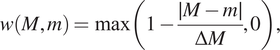 $$ w\left(M,m\right)=\max \left(1-\frac{\mid M-m\mid }{\Delta M},0\right), $$
where the positive parameter $ \Delta M $
determines the width of the function’s support. Many other functional forms could be used. Following,(Reference Bull and Byrne
48
) we use a triangular kernel due to the simplicity of the relationship between
$ \Delta M $
determines the width of the function’s support. Many other functional forms could be used. Following,(Reference Bull and Byrne
48
) we use a triangular kernel due to the simplicity of the relationship between $ \Delta M $
and the support of the weighting function (any marks more than
$ \Delta M $
and the support of the weighting function (any marks more than $ \Delta M $
from the target mark have weight 0). We note that other kernels, such as a Gaussian kernel, could also be used, but that those that have compact support,
$ \Delta M $
from the target mark have weight 0). We note that other kernels, such as a Gaussian kernel, could also be used, but that those that have compact support, $ w\left(M,M\right)=1 $
and
$ w\left(M,M\right)=1 $
and $ w\left(M,m\right)\in \left[0,1\right] $
, are likely to be most informative. Choosing an appropriate value for
$ w\left(M,m\right)\in \left[0,1\right] $
, are likely to be most informative. Choosing an appropriate value for $ \Delta M $
is important, and depends on the range over which the target marks vary and the desired ratio of signal to noise. In general, fixing
$ \Delta M $
is important, and depends on the range over which the target marks vary and the desired ratio of signal to noise. In general, fixing $ \Delta M\approx 0.1\times \left({M}_{\mathrm{max}}-{M}_{\mathrm{min}}\right) $
appears to provide a good balance, where
$ \Delta M\approx 0.1\times \left({M}_{\mathrm{max}}-{M}_{\mathrm{min}}\right) $
appears to provide a good balance, where $ {M}_{\mathrm{max}} $
and
$ {M}_{\mathrm{max}} $
and $ {M}_{\mathrm{min}} $
are the extremal values of the target marks (see Reference (Reference Bull and Byrne48) for details of alternative functional forms and a detailed analysis of how the choice of weighting function and
$ {M}_{\mathrm{min}} $
are the extremal values of the target marks (see Reference (Reference Bull and Byrne48) for details of alternative functional forms and a detailed analysis of how the choice of weighting function and $ \Delta M $
influence the signal to noise ratio in the resulting wPCF).
$ \Delta M $
influence the signal to noise ratio in the resulting wPCF).
The wPCF is defined as follows:
 $$ wPCF\left(r,M,{C}_1\right)=\frac{1}{N_{C_1}}\sum \limits_{i=1}^N\unicode{x1D540}\left({C}_1,{c}_i\right)\left(\sum \limits_{j=1}^N\frac{w\left(M,{m}_j\right){I}_{\left[0, dr\right)}\left(|{\mathbf{x}}_i-{\mathbf{x}}_j|-r\right)}{A_r\left({\mathbf{x}}_i\right)}/\frac{W_M}{A}\right), $$
where $ {W}_M={\sum}_{i=1}^N{w}_m\left(M,{m}_i\right) $
is the total “weight” associated with the target label
$ {W}_M={\sum}_{i=1}^N{w}_m\left(M,{m}_i\right) $
is the total “weight” associated with the target label $ M $
across all points. The wPCF extends the cross-PCF by weighting the contribution of each point based on how closely its continuous mark matches the target mark.
$ M $
across all points. The wPCF extends the cross-PCF by weighting the contribution of each point based on how closely its continuous mark matches the target mark.
We note that the wPCF can be used to compare point clouds with two continuous marks by replacing the categorical target mark $ {C}_1 $
with a second continuous mark (say,
$ {C}_1 $
with a second continuous mark (say, $ {M}_1 $
):
$ {M}_1 $
):
 $$ wPCF\left(r,{M}_1,{M}_2\right)=\frac{1}{W_{M_1}}\sum \limits_{i=1}^N{w}_1\left({M}_1,{m}_{1_i}\right)\left(\sum \limits_{j=1}^N\frac{w_2\left({M}_2,{m}_{2_j}\right){I}_{\left[0, dr\right)}\left(|{\mathbf{x}}_i-{\mathbf{x}}_j|-r\right)}{A_r\left({\mathbf{x}}_i\right)}/\frac{W_{M_2}}{A}\right). $$
In Equation (13) the weighting functions $ {w}_1 $
and
$ {w}_1 $
and $ {w}_2 $
quantify proximity to target marks
$ {w}_2 $
quantify proximity to target marks $ {M}_1 $
and
$ {M}_1 $
and $ {M}_2 $
, respectively. Note that since the ranges of the marks
$ {M}_2 $
, respectively. Note that since the ranges of the marks $ {m}_1 $
and
$ {m}_1 $
and $ {m}_2 $
may differ substantially, the functions
$ {m}_2 $
may differ substantially, the functions $ {w}_1 $
and
$ {w}_1 $
and $ {w}_2 $
may not necessarily use the same value of
$ {w}_2 $
may not necessarily use the same value of $ \Delta M $
in Equation (11) (e.g., see Reference (Reference Bull and Byrne48)).
$ \Delta M $
in Equation (11) (e.g., see Reference (Reference Bull and Byrne48)).
2.3.5.3. Example
We again use synthetic dataset I, where points with $ m<0.5 $
are on the left-hand side of the domain, and have been placed in clusters with the
$ m<0.5 $
are on the left-hand side of the domain, and have been placed in clusters with the $ {C}_1 $
cells. In contrast, points on the right-hand side have
$ {C}_1 $
cells. In contrast, points on the right-hand side have $ m>0.5 $
and cluster independently from the
$ m>0.5 $
and cluster independently from the $ {C}_1 $
clusters.
$ {C}_1 $
clusters.
Figure 4b shows $ wPCF\left(r,{C}_1,M\right) $
for the point pattern in Figure 4a, with cross sections of the wPCF shown in Figure 4c. For a given target value
$ wPCF\left(r,{C}_1,M\right) $
for the point pattern in Figure 4a, with cross sections of the wPCF shown in Figure 4c. For a given target value $ M $
, the cross sections of the wPCF can be interpreted in the same manner as the cross-PCF or PCF. Figure 4b identifies two types of correlation in the data, each associated with different values of
$ M $
, the cross sections of the wPCF can be interpreted in the same manner as the cross-PCF or PCF. Figure 4b identifies two types of correlation in the data, each associated with different values of $ m $
. For
$ m $
. For $ 0<r\approx 150 $
, there is strong short-range clustering between cells of type
$ 0<r\approx 150 $
, there is strong short-range clustering between cells of type $ {C}_1 $
and cells of type
$ {C}_1 $
and cells of type $ {C}_2 $
with
$ {C}_2 $
with $ m<0.5 $
, with weak short-range exclusion up to this length scale for
$ m<0.5 $
, with weak short-range exclusion up to this length scale for $ m>0.5 $
. Since cells on left-hand side of the domain have
$ m>0.5 $
. Since cells on left-hand side of the domain have $ 0\le m<0.5 $
, and those on the right-hand side have
$ 0\le m<0.5 $
, and those on the right-hand side have $ 0.5\le m\le 1 $
, this effect is consistent with the information from the cross-PCF and TCM above. One advantage of visualizing the wPCF as a heatmap (Figure 4b) is that it identifies threshold values of
$ 0.5\le m\le 1 $
, this effect is consistent with the information from the cross-PCF and TCM above. One advantage of visualizing the wPCF as a heatmap (Figure 4b) is that it identifies threshold values of $ M $
at which the nature of the cell–cell correlations changes, as demonstrated in Reference (Reference Bull and Byrne48).
$ M $
at which the nature of the cell–cell correlations changes, as demonstrated in Reference (Reference Bull and Byrne48).
Motivating example III: weighted-PCF. (a) Synthetic dataset I: the same point pattern from Figure 2, now shown with the continuous mark $ m $
associated with cells of type
$ m $
associated with cells of type $ {C}_2 $
. Recall cells of type
$ {C}_2 $
. Recall cells of type $ {C}_2 $
with
$ {C}_2 $
with $ 0\le x\le 500 $
have
$ 0\le x\le 500 $
have $ 0\le m< $
0.5, while those with
$ 0\le m< $
0.5, while those with $ 500<x\le 1000 $
have
$ 500<x\le 1000 $
have $ 0.5\le m\le 1 $
. (b) The wPCF,
$ 0.5\le m\le 1 $
. (b) The wPCF, $ wPCF\left(r,{C}_1,m\right) $
, for the point pattern in panel a identifies differences in clustering between cells of type
$ wPCF\left(r,{C}_1,m\right) $
, for the point pattern in panel a identifies differences in clustering between cells of type $ {C}_1 $
and cells of type
$ {C}_1 $
and cells of type $ {C}_2 $
with marks above or below
$ {C}_2 $
with marks above or below $ m=0.5 $
. (c) Cross sections of the wPCF in panel b. These plots distinguish the strong clustering of cells of type
$ m=0.5 $
. (c) Cross sections of the wPCF in panel b. These plots distinguish the strong clustering of cells of type $ {C}_1 $
with cells of type
$ {C}_1 $
with cells of type $ {C}_2 $
that have
$ {C}_2 $
that have $ m<0.5 $
and their weak exclusion from cells of type
$ m<0.5 $
and their weak exclusion from cells of type $ {C}_2 $
that have
$ {C}_2 $
that have $ m>0.5 $
.
$ m>0.5 $
.
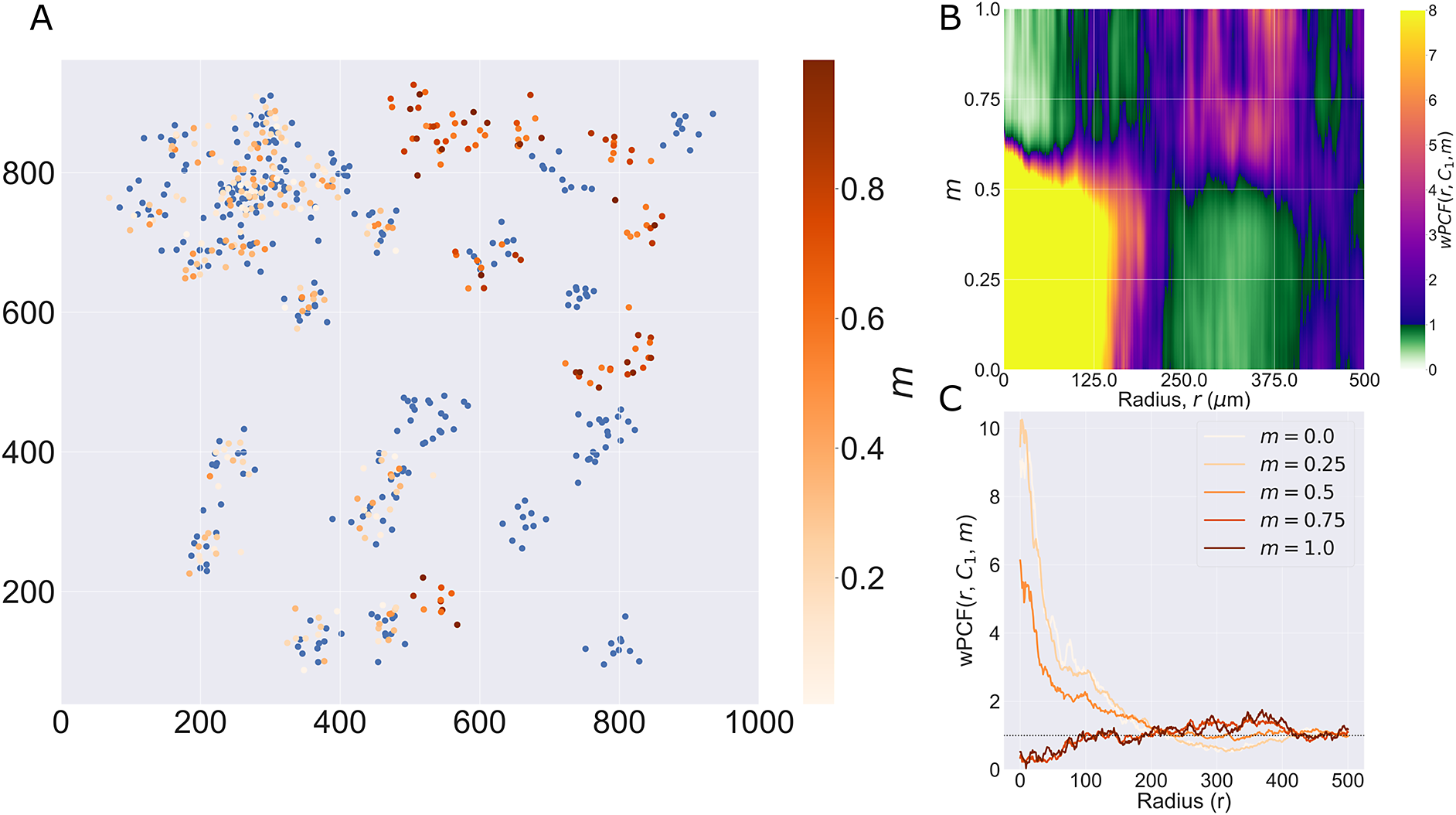
3. Results
In this section, we illustrate the utility of the TCM, NCF, and wPCF through their application to an ROI from a multiplex IHC image of a murine colorectal carcinoma (see the Methods section for details, and Section S1 of the Supplementary Material for similar analyses of three additional ROIs). Figure 5 shows the cross-PCFs that describe the pairwise correlations between all cell types present in the data. Due to the low numbers of cytotoxic and regulatory T cells, we focus subsequent analyses on relationships between epithelium and T helper cells (two abundant cell types that are spatially anticorrelated) and on T helper cells and macrophages (the most abundant immune cell subtypes, which are spatially correlated). When applying the NCF, we include neutrophils as a third immune cell subtype which colocalizes with T helper cells and macrophages.
Cross-PCFs for pairwise combinations of cell types in the ROI. Cross-PCFs for pairs of cell types from the ROI. We observe exclusion between epithelium and all immune cell subtypes, and strong pairwise correlation with macrophages, neutrophils, and T helper cells on short length scales. Results involving regulatory and cytotoxic T Cells are omitted as their cell counts are low in this ROI.
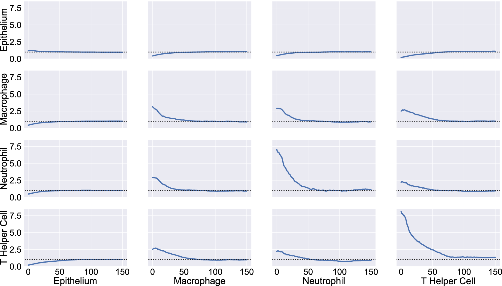
3.1. Cross-PCFs and TCMs identify colocalization and exclusion in cell center data
We first consider T helper cells (Th) and macrophages (M), which are shown to be colocalized from the cross-PCFs in Figure 5. Figure 6a shows the channels of the multiplex image that correspond approximately with T helper cells (CD4+, orange) and macrophages (CD68+, green); the cell centers of these cell populations within the ROI are shown in Figure 6b (see Figure 1 for other cell locations). In this ROI, both T helper cells and macrophages are predominantly found in the stromal tissue between islands of (cancerous) epithelial cells, leading to positive spatial correlation on short length scales ( $ 0\hskip0.35em \lesssim \hskip0.35em r\hskip0.35em \lesssim \hskip0.35em 75\hskip0.3em \mu m $
).
$ 0\hskip0.35em \lesssim \hskip0.35em r\hskip0.35em \lesssim \hskip0.35em 75\hskip0.3em \mu m $
).
PCF and TCM for positively correlated cell types. (a) Locations of T helper cells (CD4+, orange) and macrophages (CD68+, green) in the ROI (with DAPI, blue). These cell types colocalize in the tissue between epithelial cell islands. (b) Cell centers identified as T helper cells (orange) and macrophages (green). (c) Cross-PCF for T helper cells to macrophages, $ {g}_{ThM}(r) $
. These cell types are spatially colocated over a wide range of distances, that is,
$ {g}_{ThM}(r) $
. These cell types are spatially colocated over a wide range of distances, that is, $ {g}_{ThM}(r)>1 $
for
$ {g}_{ThM}(r)>1 $
for $ 0\hskip0.35em \lesssim \hskip0.35em r\hskip0.35em \lesssim \hskip0.35em 75\hskip0.3em \mu \mathrm{m} $
. (d) TCM for T helper cells to macrophages,
$ 0\hskip0.35em \lesssim \hskip0.35em r\hskip0.35em \lesssim \hskip0.35em 75\hskip0.3em \mu \mathrm{m} $
. (d) TCM for T helper cells to macrophages, $ {\Gamma}_{ThM} $
, for
$ {\Gamma}_{ThM} $
, for $ r=50\hskip0.3em \mu \mathrm{m} $
. Red regions indicate colocalization of the cell types in stromal regions, while blue regions correspond to isolated T helper cells.
$ r=50\hskip0.3em \mu \mathrm{m} $
. Red regions indicate colocalization of the cell types in stromal regions, while blue regions correspond to isolated T helper cells.
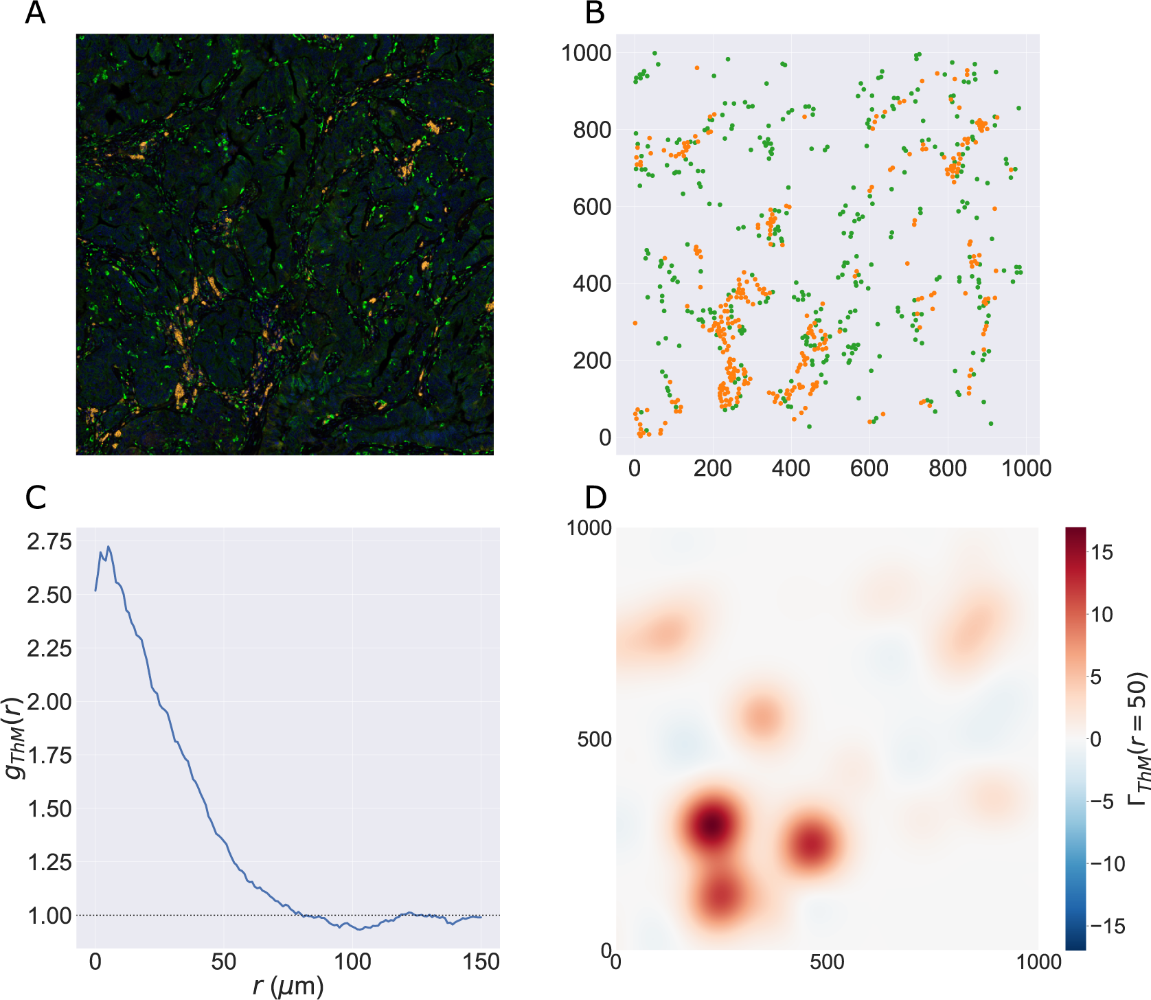
Colocalization is clearly identified by the cross-PCF in Figure 6c: for $ 0\hskip0.35em \le \hskip0.35em r\hskip0.35em \lesssim \hskip0.3em 75 $
,
$ 0\hskip0.35em \le \hskip0.35em r\hskip0.35em \lesssim \hskip0.3em 75 $
, $ {g}_{ThM}(r)>1 $
, indicating clustering between the cells of up to 2.75 times greater than expected under CSR, on length scales up to approximately
$ {g}_{ThM}(r)>1 $
, indicating clustering between the cells of up to 2.75 times greater than expected under CSR, on length scales up to approximately $ 75\hskip0.4em \mu \mathrm{m} $
(a distance approximating the width of the stromal region that separates epithelial clusters).
$ 75\hskip0.4em \mu \mathrm{m} $
(a distance approximating the width of the stromal region that separates epithelial clusters).
Figure 6d shows $ {\Gamma}_{ThM}\left(r,\mathbf{x}\right) $
for
$ {\Gamma}_{ThM}\left(r,\mathbf{x}\right) $
for $ r=50\hskip0.3em \mu \mathrm{m} $
. This permits the clustering identified by the cross-PCF to be mapped onto the ROI, revealing subregions in which T helper cells are spatially colocated with, or excluded from, macrophages. We observe strong clustering in stromal regions, with islands of weak exclusion where isolated T helper cells are present. We conclude that, while T helper cells typically colocalize with macrophages, certain subregions of the ROI that contain T helper cells have low numbers of macrophages within a
$ r=50\hskip0.3em \mu \mathrm{m} $
. This permits the clustering identified by the cross-PCF to be mapped onto the ROI, revealing subregions in which T helper cells are spatially colocated with, or excluded from, macrophages. We observe strong clustering in stromal regions, with islands of weak exclusion where isolated T helper cells are present. We conclude that, while T helper cells typically colocalize with macrophages, certain subregions of the ROI that contain T helper cells have low numbers of macrophages within a $ 50\hskip0.4em \mu \mathrm{m} $
radius. Further, these subregions do not contribute significantly to the overall correlation of T helper cells with macrophages in the cross-PCF.
$ 50\hskip0.4em \mu \mathrm{m} $
radius. Further, these subregions do not contribute significantly to the overall correlation of T helper cells with macrophages in the cross-PCF.
In Figure 7, we focus on T helper (Th) and epithelial cells (E), which are shown to be anticorrelated by the cross-PCFs in Figure 5. In Figure 7c, the cross-PCF $ {g}_{ThE}(r) $
shows exclusion for
$ {g}_{ThE}(r) $
shows exclusion for $ 0\le r\hskip0.35em \lesssim \hskip0.35em 75 $
, with the strongest exclusion occurring on small length scales. This exclusion is also identified by
$ 0\le r\hskip0.35em \lesssim \hskip0.35em 75 $
, with the strongest exclusion occurring on small length scales. This exclusion is also identified by $ {\Gamma}_{ThE}\left(r,\mathbf{x}\right) $
in Figure 7d, which shows that the cross-PCF is dominated by strong exclusion from T helper cells in the stromal islands between epithelial cells as expected. The contributions from T helper cells outside the stromal regions (e.g., those in the lower right quadrant of the ROI) are negligible compared to those in the lower left quadrant, due to the large number of T helper cells in that subregion.
$ {\Gamma}_{ThE}\left(r,\mathbf{x}\right) $
in Figure 7d, which shows that the cross-PCF is dominated by strong exclusion from T helper cells in the stromal islands between epithelial cells as expected. The contributions from T helper cells outside the stromal regions (e.g., those in the lower right quadrant of the ROI) are negligible compared to those in the lower left quadrant, due to the large number of T helper cells in that subregion.
PCF and TCM for negatively correlated cell types. (a) Locations of T helper (CD4+, orange) and epithelial cells (E-cadherin+, white) in the ROI (with DAPI, blue). Epithelial cells exist in clumped “nests,” with T helper cells restricted to the stromal regions between them. (b) Cell centers of T helper cells (orange) and epithelial cells (blue). (c) PCF for T helper cells to epithelial cells, $ {g}_{ThE}(r) $
. We observe strong spatial exclusion, as
$ {g}_{ThE}(r) $
. We observe strong spatial exclusion, as $ {g}_{ThE}(r)<1 $
for
$ {g}_{ThE}(r)<1 $
for $ r\hskip0.35em \lesssim \hskip0.35em 75 $
. (d) TCM for T helper cells to epithelial cells,
$ r\hskip0.35em \lesssim \hskip0.35em 75 $
. (d) TCM for T helper cells to epithelial cells, $ {\Gamma}_{ThE}\left(r,\mathbf{x}\right) $
, for
$ {\Gamma}_{ThE}\left(r,\mathbf{x}\right) $
, for $ r=50\hskip0.3em \mu \mathrm{m} $
. The blue regions showing strong exclusion indicate subregions of the ROI which are devoid of epithelial cells. The strongest signals occur where T helper cells are organized in large clusters, while regions with few T helper cells do not contribute significantly to the cross-PCF.
$ r=50\hskip0.3em \mu \mathrm{m} $
. The blue regions showing strong exclusion indicate subregions of the ROI which are devoid of epithelial cells. The strongest signals occur where T helper cells are organized in large clusters, while regions with few T helper cells do not contribute significantly to the cross-PCF.
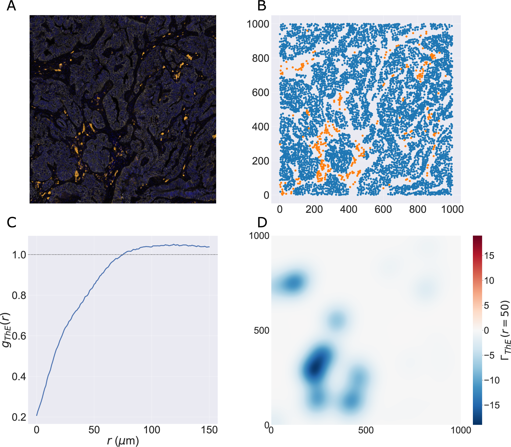
3.2. NCFs identify spatial correlations between three cell types simultaneously
Figure 8 shows the NCF for macrophages, T helper cells, and neutrophils (spatial locations shown in Figure 8a). We calculate the smallest circles enclosing each triplet containing one of each cell type, and note their radii. Figure 8b compares the number of circles with radius $ r $
observed in the data, with the expected number if macrophages, neutrophils and T helper cells are randomly distributed (obtained via simulation as described in the methods, for
$ r $
observed in the data, with the expected number if macrophages, neutrophils and T helper cells are randomly distributed (obtained via simulation as described in the methods, for $ M={10}^8 $
). More circles are observed than expected under CSR. By taking the ratio of the curves in Figure 8b, we generate the NCF in Figure 8c. The NCF shows that triplets comprising a macrophage, a neutrophil and a T helper cell are up to 35 times more likely to cluster within a neighbourhood of radius 0–
$ M={10}^8 $
). More circles are observed than expected under CSR. By taking the ratio of the curves in Figure 8b, we generate the NCF in Figure 8c. The NCF shows that triplets comprising a macrophage, a neutrophil and a T helper cell are up to 35 times more likely to cluster within a neighbourhood of radius 0– $ 20\hskip0.3em \mu \mathrm{m} $
than would be expected if the cells were randomly distributed. We conclude that these cell types are frequently found together.
$ 20\hskip0.3em \mu \mathrm{m} $
than would be expected if the cells were randomly distributed. We conclude that these cell types are frequently found together.
The NCF identifies spatial colocalization between three cell types. (a) Locations of T helper cells (orange), macrophages (green), and neutrophils (purple) extracted from the ROI. All three cell types are found in stromal regions, while macrophages and neutrophils are more likely to be observed within the epithelial islands (e.g., in the top left corner). (b) Expected and observed numbers of circles of radius $ r $
. (c) NCF obtained by computing the ratio of the curves in panel b,
$ r $
. (c) NCF obtained by computing the ratio of the curves in panel b, $ {\mathrm{NCF}}_{ThMN}(r) $
. For
$ {\mathrm{NCF}}_{ThMN}(r) $
. For $ r\hskip0.35em \lesssim \hskip0.35em 75\hskip0.3em \mu \mathrm{m} $
, neutrophils, macrophages, and T helper cells are colocalized within a circle of radius
$ r\hskip0.35em \lesssim \hskip0.35em 75\hskip0.3em \mu \mathrm{m} $
, neutrophils, macrophages, and T helper cells are colocalized within a circle of radius $ r $
more often than would be expected under CSR.
$ r $
more often than would be expected under CSR.

3.3. The wPCF identifies correlations without classification or segmentation
Recall that in order to apply the PCF, cross-PCF, TCM, and NCF, the multiplex imaging data must be segmented and then classified to identify cell centers and assign them categorical labels (or cell types). We now show how the wPCF can be applied directly to multiplex imaging data to identify spatial correlations, without segmentation or classification.
Figure 9 demonstrates that the wPCF can identify correlations when some cells are not classified. Rather than specifying a threshold value of the CD4 marker intensity to identify CD4+ cells, we instead view the average CD4 intensity of each cell as a continuous mark. Figure 9a shows epithelial cells determined by specifying a threshold, while Figure 9b shows all cells labeled according to their average CD4 intensity. The wPCF calculated in panel c shows that the spatial positions of cells with low CD4 intensity differ from those with high CD4 expression (with $ \Delta M=2 $
in Equation (11)). Figure 9c,d shows that cells with mean CD4 intensity below approximately 4 are not strongly correlated with epithelial cells. However, for larger values of CD4 intensity, the profiles of the wPCF are in good agreement with the cross-PCF
$ \Delta M=2 $
in Equation (11)). Figure 9c,d shows that cells with mean CD4 intensity below approximately 4 are not strongly correlated with epithelial cells. However, for larger values of CD4 intensity, the profiles of the wPCF are in good agreement with the cross-PCF $ {g}_{ThE}(r) $
(shown as a red dashed line in Figure 9d).
$ {g}_{ThE}(r) $
(shown as a red dashed line in Figure 9d).
The wPCF identifies correlation between epithelial cells and cells with different CD4 expression levels. (a) Epithelial cell centers. (b) Cell centers labeled according to the average CD4 stain intensity within each cell. (c) wPCF ( $ r $
,
$ r $
, $ E $
, CD4), showing clear qualitative and quantitative differences in colocalization with epithelial cells as CD4 expression levels vary. (d) Cross sections of the wPCF in panel c. Points with low CD4 expression have a different pattern of correlation than those with higher expression. The profile for cells with high CD4 expression corresponds to the cross-PCF
$ E $
, CD4), showing clear qualitative and quantitative differences in colocalization with epithelial cells as CD4 expression levels vary. (d) Cross sections of the wPCF in panel c. Points with low CD4 expression have a different pattern of correlation than those with higher expression. The profile for cells with high CD4 expression corresponds to the cross-PCF $ {g}_{ThE}(r) $
, calculated for cells which have been manually classified as T helper cells (red dashed line). Cells with low CD4 intensity colocalize with epithelial cells, likely due to many epithelial cells having low CD4 expression. Cells with higher expression of CD4 are anticorrelated with epithelial cells for
$ {g}_{ThE}(r) $
, calculated for cells which have been manually classified as T helper cells (red dashed line). Cells with low CD4 intensity colocalize with epithelial cells, likely due to many epithelial cells having low CD4 expression. Cells with higher expression of CD4 are anticorrelated with epithelial cells for $ 0\le r\hskip0.35em \lesssim \hskip0.35em 75 $
.
$ 0\le r\hskip0.35em \lesssim \hskip0.35em 75 $
.
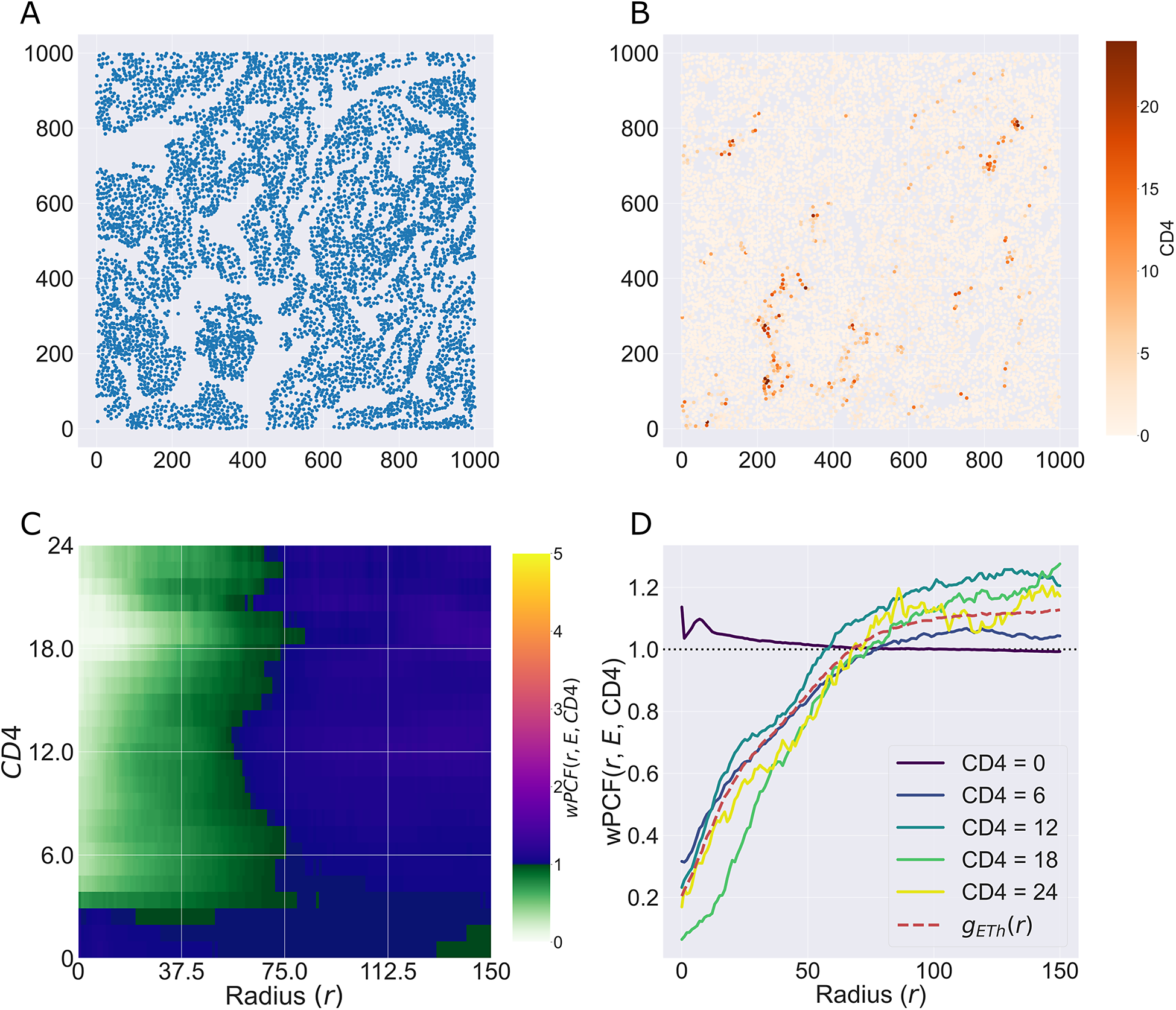
Finally, in Figure 10, we show that application of the wPCF to multiplex images, without cell segmentation or classification, can identify spatial correlation. Panels a and b show points from a regular lattice sampled from the multiplex image of the ROI, at a resolution of 1 point every $ 5\hskip0.3em \mu \mathrm{m} $
. In panel a, points are labeled according to a thresholded value of the epithelial cell marker, while in panel b, they are labeled according to the CD4 intensity at that pixel (note we use the notation “Opal 520,” the marker associated with CD4 cells, to distinguish these raw pixel intensities from the mean pixel intensities used in Figure 9). The wPCF which compares these marks is shown in panel c, and is in good qualitative and quantitative agreement with the wPCF from Figure 9 (with
$ 5\hskip0.3em \mu \mathrm{m} $
. In panel a, points are labeled according to a thresholded value of the epithelial cell marker, while in panel b, they are labeled according to the CD4 intensity at that pixel (note we use the notation “Opal 520,” the marker associated with CD4 cells, to distinguish these raw pixel intensities from the mean pixel intensities used in Figure 9). The wPCF which compares these marks is shown in panel c, and is in good qualitative and quantitative agreement with the wPCF from Figure 9 (with $ \Delta M=20 $
in Equation (11)). We conclude that applying the wPCF directly to pixels and stain intensities can identify the same spatial patterns of clustering and exclusion as those identified by the cross-PCF, without cell segmentation or classification.
$ \Delta M=20 $
in Equation (11)). We conclude that applying the wPCF directly to pixels and stain intensities can identify the same spatial patterns of clustering and exclusion as those identified by the cross-PCF, without cell segmentation or classification.
wPCF identifies correlation between epithelial cells and pixels with varying CD4 expression. The results from Figure 9 are recovered when the wPCF is calculated from points sampled from the original multiplex image using a regular $ 5\hskip0.3em \mu \mathrm{m} $
lattice, showing that the spatial correlation between T helper cells and epithelial cells can be identified without segmentation or classification. (a) Pixel intensities of the Opal 520 marker (associated with CD4), sampled across the ROI on a regular
$ 5\hskip0.3em \mu \mathrm{m} $
lattice, showing that the spatial correlation between T helper cells and epithelial cells can be identified without segmentation or classification. (a) Pixel intensities of the Opal 520 marker (associated with CD4), sampled across the ROI on a regular $ 5\hskip0.3em \mu \mathrm{m} $
lattice. (b) Pixels marked as Opal 780 positive (associated with epithelial cells), determined via thresholding, sampled across the ROI on a regular
$ 5\hskip0.3em \mu \mathrm{m} $
lattice. (b) Pixels marked as Opal 780 positive (associated with epithelial cells), determined via thresholding, sampled across the ROI on a regular $ 5\hskip0.3em \mu \mathrm{m} $
lattice. (c) wPCF describing correlation between pixels positive for Opal 780 and the pixel intensity of Opal 520. (d) Cross sections of the wPCF in panel c have the same shape as the cross-PCF in panel d for pixels with high CD4 intensity.
$ 5\hskip0.3em \mu \mathrm{m} $
lattice. (c) wPCF describing correlation between pixels positive for Opal 780 and the pixel intensity of Opal 520. (d) Cross sections of the wPCF in panel c have the same shape as the cross-PCF in panel d for pixels with high CD4 intensity.
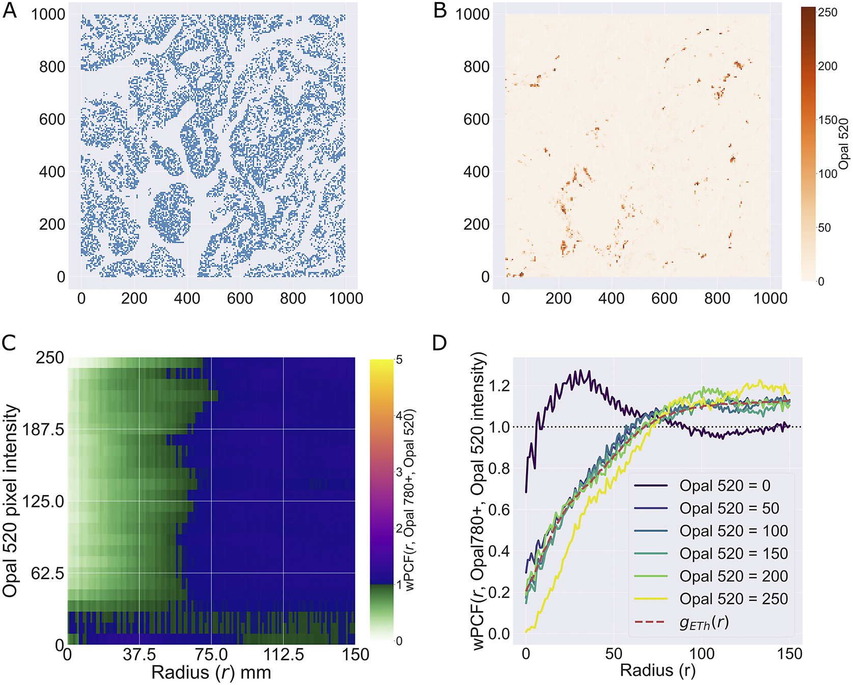
4. Discussion
Multiplex images contain a wealth of spatial information, and have the potential to greatly increase the information that can be extracted from histological samples. Each image provides a high-resolution map of cell locations across tissue samples that may contain millions of cells, together with detailed information about their phenotypes and morphology. As multiplex images become more widespread and as digital tools for their visualization and analysis improve, the demand for automated methods that can extract detailed spatial information from them is increasing. Such methods should be agnostic to the technology used to generate the images, the disease under investigation, and the particular markers with which the sample has been stained.
Many existing methods can extract information from multiplex images. One popular approach involves using AI or machine learning approaches to identify correlations between features extracted from multiplex images and clinically relevant features such as disease progression. AI methods can be extremely powerful, but are not ideally suited to all situations. In particular, an AI algorithm may require vast numbers of images for use as training data. Further, the tissue type and panel of markers chosen for staining should be consistent across the training data, thereby reducing the applicability of the algorithm to samples from different diseases (e.g., an algorithm trained on multiplex images of immune cells in colorectal cancer cannot reliably be applied to images of immune cells in prostate cancer, or to images of stromal cells in colorectal cancer). AI methods can sometimes lack interpretability, making it difficult to understand which features of an image an algorithm is using and to understand when errors are likely to arise.
On the other hand, a range of statistical and mathematical methods can also describe features of multiplex images in an interpretable way. These methods may derive from a range of disciplines, such as network science, TDA, and spatial statistics. They provide quantitative descriptions of specific spatial features of an image; for example, ecological analyses may describe correlations in cell counts across subregions of an ROI with a fixed area, quantifying the strength of local correlations.(Reference Gatenbee, Baker and Schenck 29 ) Existing metrics have typically been developed to address a specific problem. As a result, multiple methods may be used to describe the same features of a point pattern. For instance, the field of spatial statistics encompasses a range of methods designed to identify correlations in point patterns, with specialized tools to address specific use cases. The PCF has been specialized to account for interactions between multiple classes of point (the cross-PCF), points generated from processes that vary across a region (inhomogeneous-PCF(Reference Baddeley, Møller and Waagepetersen 35 )), or points labeled with continuous marks (mark correlation functions, weighted-PCFs). Such metrics can provide detailed information about the spatial structure of multiplex images, even though they may have been developed for other types of data. In order to understand multiplex images using quantitative metrics, we propose the application of multiple statistics (which may derive from different mathematical fields), designed to quantify specific properties of the image.
In this paper, we have focused on three methods for extending the PCF that have been specifically designed for application to multiplex medical images. Each is applied here for the first time to multiplex IHC images from the Vectra Polaris system, in order to illustrate how they address limitations in the PCF. We now summarize each method in turn, focusing on their strengths and weaknesses.
4.1. Topographical correlation map
The TCM can visualize spatial correlations between pairs of cell populations across an ROI, highlighting subregions of strong positive or negative correlation that can be difficult to identify by visual inspection. The TCM can be calculated without requiring the user to estimate the intensity of an inhomogeneous point process; rather, it identifies subregions in which local interactions between the point patterns differ from those that would be obtained under homogeneous CSR. While we have used the TCM for visualization, it generates quantitative information which can be used for subsequent analysis. For example, the number and size of the local minima and maxima could be used as summary statistics to compare and classify images. The TCM can also be analyzed via a sub/super level-set filtration.(Reference Feng and Porter 60 ) This method from TDA can quantify spatial heterogeneity in heatmaps.
We note that, by design, the TCM is asymmetric (i.e., $ {\Gamma}_{ab}\left(r,\mathbf{x}\right)\ne {\Gamma}_{ba}\left(r,\mathbf{x}\right) $
). As such, care is needed when interpreting the TCM. In particular, while
$ {\Gamma}_{ab}\left(r,\mathbf{x}\right)\ne {\Gamma}_{ba}\left(r,\mathbf{x}\right) $
). As such, care is needed when interpreting the TCM. In particular, while $ {\Gamma}_{ab}\left(r,\mathbf{x}\right) $
and
$ {\Gamma}_{ab}\left(r,\mathbf{x}\right) $
and $ {\Gamma}_{ba}\left(r,\mathbf{x}\right) $
should coincide in regions of positive correlation, they may differ in regions of negative correlation. Further, regions where
$ {\Gamma}_{ba}\left(r,\mathbf{x}\right) $
should coincide in regions of positive correlation, they may differ in regions of negative correlation. Further, regions where $ {\Gamma}_{ab}\left(r,\mathbf{x}\right)\approx 0 $
cannot be used to infer the presence (or absence) of either cell type without consideration of other metrics (e.g., local cell densities).
$ {\Gamma}_{ab}\left(r,\mathbf{x}\right)\approx 0 $
cannot be used to infer the presence (or absence) of either cell type without consideration of other metrics (e.g., local cell densities).
4.2. Neighbourhood correlation function
The NCF identifies whether groups of three or more cells are found in a circular neighbourhood of radius $ r $
more or less frequently than expected under CSR. Since it requires distance calculations between
$ r $
more or less frequently than expected under CSR. Since it requires distance calculations between $ n $
cell types, the computational complexity of the NCF is at least
$ n $
cell types, the computational complexity of the NCF is at least $ O\left({N}^n\right) $
. This limits its potential application to WSIs or to identifying correlations between a large number of cell types simultaneously: although calculating each enclosing circle is fast,(Reference Megiddo
58
) as the maximum number of circles which must be calculated is
$ O\left({N}^n\right) $
. This limits its potential application to WSIs or to identifying correlations between a large number of cell types simultaneously: although calculating each enclosing circle is fast,(Reference Megiddo
58
) as the maximum number of circles which must be calculated is $ {N}_1\times \dots \times {N}_n $
(where
$ {N}_1\times \dots \times {N}_n $
(where $ {N}_i $
is the number of cells of type
$ {N}_i $
is the number of cells of type $ i $
) the computational effort involved increases rapidly as the total number of cells and number of cell types increase. As for the PCF, the runtime performance of the algorithm can be improved by calculating the NCF up to a maximal neighbourhood size of interest
$ i $
) the computational effort involved increases rapidly as the total number of cells and number of cell types increase. As for the PCF, the runtime performance of the algorithm can be improved by calculating the NCF up to a maximal neighbourhood size of interest $ r $
; this reduces the number of
$ r $
; this reduces the number of $ n $
-wise maximum enclosing circles that must be calculated (any combination of points containing a pair separated by more than the length scale of interest can be immediately discarded). The NCF also relies on repeated sampling of random data to identify the expected number of neighbourhoods that would be observed under CSR. For a given region, this probability can be calculated in advance to an arbitrary level of precision, and becomes more accurate with more samples. However, more research is needed to determine the minimum number of samples needed to achieve a given accuracy.
$ n $
-wise maximum enclosing circles that must be calculated (any combination of points containing a pair separated by more than the length scale of interest can be immediately discarded). The NCF also relies on repeated sampling of random data to identify the expected number of neighbourhoods that would be observed under CSR. For a given region, this probability can be calculated in advance to an arbitrary level of precision, and becomes more accurate with more samples. However, more research is needed to determine the minimum number of samples needed to achieve a given accuracy.
The process of calculating the NCF suggests that in future work it could be adapted to produce a spatially-resolved map, similar to the TCM, which would indicate areas of an ROI in which $ n $
cells of interest colocalize. For example, Figure 3c,g suggest that placing a kernel on each neighbourhood which is weighted inversely to the radius of the circle would generate a landscape in which colocalization of multiple populations would be identified at local maxima.
$ n $
cells of interest colocalize. For example, Figure 3c,g suggest that placing a kernel on each neighbourhood which is weighted inversely to the radius of the circle would generate a landscape in which colocalization of multiple populations would be identified at local maxima.
4.3. Weighted-PCF
The wPCF generalizes the cross-PCF to data with continuous labels (e.g., cell centers that have not been classified into discrete categories, or to pixels which have not been segmented to find cell centers). As such it can be calculated without classification or cell segmentation preprocessing steps. However, this also increases the number of “parameters” required. In particular, the choice of weighting function determines the ratio of signal/noise identified by the wPCF and must be considered in advance (see Reference (Reference Bull and Byrne48) for a detailed examination of the impact of varying the weighting function on the wPCF). The tuning parameters used to construct the wPCF are in some ways similar to those used to perform cell classification (e.g. threshold values for stain intensities). Since it requires careful choice of the weighting function and associated parameters, users should carefully consider the most appropriate choice of method for comparing their data, since depending on the context methods designed to directly compare random fields of intensities may be more appropriate than the point process setting (see, e.g., Reference (Reference Lagache, Sauvonnet, Danglot and Olivo-Marin61) for a detailed comparison of some relevant pixel-based and object-based methods for quantifying colocalization).
There is considerable scope for developing approaches to interpret the wPCF. The heatmap that it generates can be analyzed using techniques similar to those discussed for the TCM above. Further, since the wPCF generates outputs comparable to a series of cross-PCFs with different target marks, it may be possible to define an analogue of the TCM in order to localize regions in which the populations of interest colocalize. For example, a similar kernel method to that defined for the TCM could be used, in which kernels are scaled both by strength of colocalization (as in the current implementation) and by the weighting of the point relative to the target mark in the wPCF.
It is also possible to use the outputs from the wPCF to create a vectorized “spatial signature” which can be used to cluster regions which have similar spatial structures.(Reference Bull and Byrne 48 ) Such an approach could be used to automatically identify regions with similar spatial cellular interactions, or which contain spatial patterns associated with, for example, cancer progression or disease severity. Indeed, by vectorizing the spatial descriptors described within this paper the approach described in Reference (Reference Bull and Byrne48) to identify such “spatial biomarkers” could be extended.
4.4. Conclusions
Multiplex images contain vast amounts of spatial information which can be exploited using quantitative techniques. The spatial statistics considered in this paper represent one approach to analyzing these data, and benchmarking studies that compare the efficiency and insight of different methods are needed. There are several challenges associated with applying methods based on spatial statistical analysis of point patterns, such as those described in this paper, to large regions, such as whole slide images, or images with large numbers of different cell types (e.g., 60+). One major limitation relates to their scaling as the number of cells increases (see Supplementary Material), since WSIs may contain millions of individual cells. Improvements in the efficiency of code implementation are likely to be needed in these cases, such as parallelizing calculations or restricting the number of pairwise distance calculations that must be performed by introducing distance thresholds.
The methods described in this paper were designed to exploit the spatial information contained in multiplex images. We note, however, that they can be applied to multiple imaging modalities and multiple diseases. Equally, each method can be applied to generic point cloud data from contexts outside of biology.
We have previously shown that combining spatial statistics can generate more comprehensive descriptions of point data than individual metrics alone.(Reference Bull, Macklin and Quaiser 38 , Reference Bull and Byrne 48 ) In future work, we will determine how complementary methods from mathematical fields such as spatial statistics, network science, and topology, can build upon this to provide a rigorous quantitative description of how data are spatially distributed.
Supplementary material
The supplementary material for this article can be found at http://doi.org/10.1017/S2633903X24000011.
Data availability statement
Python code for reproducing the results described in this paper, along with the relevant data, is available on github at https://github.com/JABull1066/ExtendedCorrelationFunctions.
Author contributions
Conceptualization: J.A.B. Methodology: J.A.B., E.J.M., S.J.L., and H.M.B. Data curation: J.A.B. and E.J.M. Data visualization: J.A.B. and E.J.M. Investigation: J.A.B., E.J.M., S.J.L., and H.M.B. Writing original draft: J.A.B., E.J.M., S.J.L., and H.M.B. All authors approved the final submitted draft.
Funding statement
J.A.B. was supported by Cancer Research UK (CR-UK) grant number CTRQQR-2021\100002, through the Cancer Research UK Oxford Centre. E.J.M. was supported by the Lee Placito Medical Research Fund (University of Oxford), and by CR-UK grant number C5255/A18085, through the Cancer Research UK Oxford Centre. S.J.L. was supported by CR-UK grant number DRCNPG-Jun22\100002.
Competing interest
The authors declare no competing interests exist.
Ethical standards
The research meets all ethical guidelines, including adherence to the legal requirements of the study country.


 Open access