


Impact Statement
In recent decades, single-particle tracking analysis has become a powerful method to evaluate biomolecules’ diffusion dynamics and interactions in living cellular ecosystems. Because changes in biomolecule dynamics can lead us to understand either functional states or signaling pathways, this tool allows characterizing the mechanisms of one molecule at a time within single trajectories by extracting mobility-related properties together with performing mean-squared displacement approaches to quantitatively analyze diffusion, thus getting further track classification. Here, we present TrackAnalyzer, a new open-source plugin that extends from TrackMate’s single-particle tracking analysis broadly applicable under ImageJ or Fiji, which prevents users from using complex instruments and provides intuitive data analysis schemes hence leading users to a proper interpretation of information extracted from trajectories.
1. Introduction
With the development of breakthrough live-cell imaging techniques in optical microscopy, such as confocal and total Internal reflection microscopy (TIRF) over the last 40 years, quantitative analysis of dynamic processes at the subcellular level has become crucial to acquire valuable information related to dynamics intracellular processes over long periods of time with a spatial resolution of a few tens of nanometers(Reference Vera, Biswas, Senecal, Singer and Park 1 ). In this context, due to advances in fluorescent protein labeling and software, single-particle tracking (SPT) analysis as a time-lapse imaging tool has become standard in life sciences to measure motion, diffusion properties, and the changing spatial distribution of single-particles in real-time with high-temporal resolution and high signal-to-noise ratio(Reference Cui, Yu, Yao, Xing, Lin and Li 2 ). As particles are fluorescently labeled, SPT analysis must seek to roughly reconstruct the motion of single particles of interest over consecutive time points. Its combination with markers allows monitoring of vital cellular processes such as cell differentiation(Reference Kok, Hebert and Huelsz-Prince 3 ). The estimation of frame-to-frame correspondence among particles at the cellular and molecular levels (with high accuracy and high reproducibility) requires a high signal-to-noise ratio. However, this is not always achieved due to severe noise from a fluctuating background, autofluorescence, blinking, photobleaching, phtototoxicity(Reference Hilsenbeck, Schwarzfischer and Skylaki 4 ), poor contrast, extremely high particle density, or motion heterogeneity. To address these challenging events, inherent to the dynamic organization of cellular components (and essential for many biological processes) such as cell division, differentiation, cell adhesion, or migration(Reference Manzo and Garcia-Parajo 5 ), SPT algorithms explicitly take some countermeasures to guarantee the correct tracking of these fluorescent particles. Specifically: (I) gap-closing events when a single particle temporarily disappears from focus and reappears later; this type of event is closely related to fluorophore blinking and stochastic fluctuations of spot or cell intensity so the tracker algorithm may bridge missing detections in a predefined number of subsequent frames(Reference Kuhn, Hettich, Davtyan and Gebhardt 6 ); (II) merging events when two single particles approach each other and fuse into a unique object; (III) splitting events when a single-particle splits into two new single-particles(Reference Jaqaman, Loerke and Mettlen 7 ). To correctly compute trajectories, single-particle candidates considered as relevant must be accurately detected and isolated from each other and from a background with nanometer spatial and millisecond temporal resolution(Reference Rahm, Malkusch, Endesfelder, Dietz and Heilemann 8 ). Thus, enhancing the signal-to-noise ratio is mandatory; the higher the background noise, the more distorted the tracking. SPT analysis involves spatial methods for (I) single-particle detection in which each spot or cell is segmented, identified, located, and isolated from the background establishing X–Y–Z–T coordinate correspondences frame-by-frame, and temporal methods for (II) single-particle linking in which each single-particle detected is assigned over time into a single track.
While manual SPT of biological processes may be straightforward when the particle density is low, tracking large datasets of sparse living cells is often a subjective, barely reproducible, and tedious task. Consequently, its automation is very much appreciated. Due to experimental constraints, fully automated SPT approaches frequently perform poorly when the experimental conditions change. For this reason, the possibility of combining automation with user control(Reference Aragaki, Ogoh, Kondo and Aoki 9 ) may facilitate the quantification of live cell events. At present, there is still a lack of user-friendly and comprehensive software for SPT to cope with the enormous amount of time-lapse microscopy acquisitions arising from quite different experimental conditions. Given the current situation, we decided to construct TrackAnalyzer to allow the user to set up sophisticated SPT analyses tailored to his/her experimental conditions, apply this analysis in batch mode to a large collection of similar acquisitions, and finally analyze the results. Our software is available through an open-source plugin for Fiji(Reference Schindelin, Arganda-Carreras and Frise 10 ) or ImageJ(Reference JSchindelin, Rueden, Hiner and Eliceiri 11 ). TrackAnalyzer performs the detection of the spots or cells to follow, the construction of the tracks, quantitative diffusion analysis, trajectory analysis, cluster size analysis, and single-step photobleaching analysis (see Figure 1). Our viewer allows 2D visualization of the spots (or cells) and tracks, spot/track filtering, and classification into user-defined specific spot/track types.
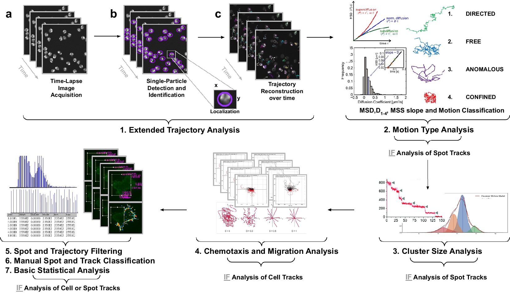
Figure 1. Illustration of the workflow to perform single particle tracking together with subsequent analysis of diffusion using TrackAnalyzer software which consists of several processes. (Reference Vera, Biswas, Senecal, Singer and Park1) Extended Trajectory Analysis. (a) After Acquisition time series of multi-movie data sets. (b) Localization, detection, and subsequent identification of single particles frame by frame. A wide range of features is extracted based on the location, radius, and image data. (c) Single particles are linked to building trajectories over time (single-particle tracking). (Reference Cui, Yu, Yao, Xing, Lin and Li2) Motion Type Analysis. The resulting trajectories and links are analyzed after the tracking step to characterize them and evaluate the type of motion by applying quantitative analysis of diffusion, mean square displacement (MSD), and moment scaling spectrum (MSS) slope. (Reference Kok, Hebert and Huelsz-Prince3) Cluster Size Analysis. The number of receptors per spot is calculated by applying Gaussian Mixture Model fitting and Single-step Photobleaching Analyses. (Reference Hilsenbeck, Schwarzfischer and Skylaki4) Chemotaxis and Migration Analysis. Several quantitative and statistical features (center of mass, forward migration indices, velocity, …) are calculated to characterize trajectories. (Reference Manzo and Garcia-Parajo5) Spot and Trajectory Filtering, (Reference Kuhn, Hettich, Davtyan and Gebhardt6) Manual Spot and Track Classification, and (Reference Jaqaman, Loerke and Mettlen7) Basic Statistical Analysis. Features extracted from spots and tracks will be used to either filter or classify them depending on user-defined conditions.
For detecting and constructing the tracks, our software takes advantage of the previously published open-source software TrackMate(Reference Tinevez, Perry and Schindelin 12 ), which is an extensible platform running for either Fiji or ImageJ, openly available and very well-documented. TrackMate provides algorithms for spot or cell detection, track construction (automated, semi-automated, and manual tracking), visualization, and subsequent feature extraction. In this way, TrackMate addresses both usability and flexibility to provide users with a user-friendly tool to tackle the complexity of this type of analysis.
For the classification of the different types of trajectories, we use TraJClassifer(Reference Wagner, Kroll, Haramagatti, Lipinski and Wiemann 13 ). This software classifies trajectories into their respective motion types: normal diffusion (ND), anomalous diffusion (AD), confined diffusion (CD), and directed motion (DM). An interesting feature of TraJClassifier is that trajectories can be divided into segments, and the motion type of each segment can be analyzed.
TrackAnalyzer implements an algorithm to calculate the diffusion coefficients of each trajectory. The algorithm is based on the mean-square-displacement (MSD) curve as a function of the time lag of each trajectory (see Section 5 in Materials and Methods). The short-time lag diffusion coefficient ( $ {D}_{1-4} $
) is also calculated by fitting the first user-defined points of the MSD curve(Reference Manzo and Garcia-Parajo
5
). MSD-based methods are reliable for short trajectories, but they may be error-prone in longer trajectories due to their nonlinearity and lack of distinction between modes of motion(Reference Ewers, Smith, Sbalzarini, Lilie, Koumoutsakos and Helenius
14
). To overcome this nonlinearity and describe nonlinear diffusion, the anomalous exponent or alpha value (
$ {D}_{1-4} $
) is also calculated by fitting the first user-defined points of the MSD curve(Reference Manzo and Garcia-Parajo
5
). MSD-based methods are reliable for short trajectories, but they may be error-prone in longer trajectories due to their nonlinearity and lack of distinction between modes of motion(Reference Ewers, Smith, Sbalzarini, Lilie, Koumoutsakos and Helenius
14
). To overcome this nonlinearity and describe nonlinear diffusion, the anomalous exponent or alpha value ( $ \alpha $
) is calculated by the power-law form of the MSD, indicating the nonlinear relationship of the MSD with time(Reference Ferrari, Manfroi and Young
15
). The exponent of this power function determines whether the motion is confined (0<
$ \alpha $
) is calculated by the power-law form of the MSD, indicating the nonlinear relationship of the MSD with time(Reference Ferrari, Manfroi and Young
15
). The exponent of this power function determines whether the motion is confined (0< $ \alpha $
<0.6), anomalous (0.6<
$ \alpha $
<0.6), anomalous (0.6< $ \alpha $
<0.9), free (0.9<
$ \alpha $
<0.9), free (0.9< $ \alpha $
<1.1), or directed (
$ \alpha $
<1.1), or directed ( $ \alpha $
>1.1)(Reference Manzo and Garcia-Parajo
5
). For long trajectories, the moment scaling spectrum (MSS) together with its slope (
$ \alpha $
>1.1)(Reference Manzo and Garcia-Parajo
5
). For long trajectories, the moment scaling spectrum (MSS) together with its slope ( $ {S}_{\mathrm{MSS}} $
) is introduced as a method to categorize the various modes of motion(Reference Manzo and Garcia-Parajo
5
). While MSD-based analysis uses only the second moment, which can mislead in judging the type of motion, MSS uses higher-order moments of the displacements. In this way, an
$ {S}_{\mathrm{MSS}} $
) is introduced as a method to categorize the various modes of motion(Reference Manzo and Garcia-Parajo
5
). While MSD-based analysis uses only the second moment, which can mislead in judging the type of motion, MSS uses higher-order moments of the displacements. In this way, an $ {S}_{\mathrm{MSS}} $
value of 0.5 defines Brownian or free motion, and
$ {S}_{\mathrm{MSS}} $
value of 0.5 defines Brownian or free motion, and $ {S}_{\mathrm{MSS}} $
values below and above 0.5 determine confined and DM, respectively. Finally, a
$ {S}_{\mathrm{MSS}} $
values below and above 0.5 determine confined and DM, respectively. Finally, a $ {S}_{\mathrm{MSS}} $
of 0 determines immobility(Reference Ewers, Smith, Sbalzarini, Lilie, Koumoutsakos and Helenius
14
).
$ {S}_{\mathrm{MSS}} $
of 0 determines immobility(Reference Ewers, Smith, Sbalzarini, Lilie, Koumoutsakos and Helenius
14
).
TrackAnalyzer also analyzes the spot or cell intensities along the whole trajectory. At this point, we provide the user with different algorithms to estimate the background fluorescence intensity described in Section 5.2 and use this estimated value to correct the raw measurement observed in the acquired images. This approach allows the identification of photobleaching. In combination with this approach, this tool provides an alternative strategy to evaluate the cluster size by fitting a Gaussian mixture model to the histogram of the logarithm of the background-subtracted integrated spot intensities.
Finally, we have also integrated the Chemotaxis and Migration Tool(Reference Zantl and Horn 16 ) to quantify both chemotaxis and migration experiments.
2. Results
2.1. Overview of the analysis procedure
The analysis workflow starts with the user calling TrackMate and setting up an analysis in this tool that correctly identifies the spots or cells and tracks in the specific experimental conditions of the dataset. TrackMate offers state-of-the-art segmentation and trajectory construction algorithms. After setting up the analysis, TrackMate will produce an XML file with the analysis parameters (this file also contains the results of the video analyzed, although these specific results are not of interest in our context of automated analysis of a collection of videos). The input to our software is the XML file produced by TrackMate, with the analysis parameters and the directory with the videos to be analyzed in batch mode. For each video in the input directory, we will create an output directory with the results of all the different analyses on that video (Figure 2). Before launching the analysis in batch mode, the user must choose the parameters for all the different kinds of analyses performed on the tracks detected by TrackMate. Specifically:
-
1. Extended trajectory analysis. We provide a number of tools that help to extend the spot and trajectory analysis offered by TrackMate. In particular, the user may choose a specific frame range so that all spots detected out of this range are excluded. The user may also exclude all spots detected outside of a cell. We also offer different output options such as generating a summary file for each video, exporting the results in XML, text file, or as a RoiSet that can be handled by ImageJ’s RoiManager. Finally, the user may choose any XY scatter plot with information coming from the detected spots or cells, links, or tracks-related features (Figure 3).
-
2. Motion-type analysis. TrackAnalyzer offers several ways of analyzing the motion type of the different trajectories. As a result, we classify trajectories into immobile or mobile depending on the threshold set by the user, and within these into confined, anomalous, free or Brownian, or directed trajectories. We calculate the short-time lag diffusion coefficient ( $ {D}_{1-4} $
),MSD, and diffusion coefficient for all trajectories (the formal definition of all these quantities are given in Section 5.1). These measurements are especially well-suited to short trajectories and characterize the movement’s onset. Additionally, trajectories are classified into short and long trajectories, depending on a threshold given by the user. Long trajectories are further analyzed using the MSS, better suited to account for their nonlinearities. Finally, we have also integrated TraJClassifier that allows the local classification of the trajectory motion type, that is, a spot may behave in one way during the first half of the trajectory and in another way in the second half. TraJClassifier’s classification is based on a random forest trained on simulated data with different kinds of motion.
$ {D}_{1-4} $
),MSD, and diffusion coefficient for all trajectories (the formal definition of all these quantities are given in Section 5.1). These measurements are especially well-suited to short trajectories and characterize the movement’s onset. Additionally, trajectories are classified into short and long trajectories, depending on a threshold given by the user. Long trajectories are further analyzed using the MSS, better suited to account for their nonlinearities. Finally, we have also integrated TraJClassifier that allows the local classification of the trajectory motion type, that is, a spot may behave in one way during the first half of the trajectory and in another way in the second half. TraJClassifier’s classification is based on a random forest trained on simulated data with different kinds of motion. -
3. Cluster size analysis. This analysis tries to estimate the number of fluorophores at each spot. This information is very useful for identifying the presence of monomers, dimers, trimers, etc., within a cluster. An unbiased estimate should account for the background fluorescence, which must be subtracted before further analysis. TrackAnalyzer offers several methods to estimate the background, described in Section 5.2. In particular, we use the following two methods to estimate the number of fluorophores:
-
a. a Gaussian mixture model fit of the histogram of the logarithm of the background-subtracted integrated spot intensities.
-
b. a single-step photobleaching analysis. This technique analyzes the time evolution of the fluorescence of an individual spot along its trajectory. The number of photobleaching steps over time is a lower bound of the number of fluorophores in the spot.
4. Chemotaxis and migration analysis. The identified trajectories can be subjected to a chemotactic and migration analysis (as implemented by the Chemotaxis and Migration tool of ImageJ(Reference Zantl and Horn 16 , Reference Zengel, Nguyen-Hoang, Schildhammer, Zantl and Kahl 17 )). This tool allows the quantitative and statistical analysis of the migration of the spot center of mass (CM) and the calculation of the forward migration indices (FMI), velocity (V), and directness (D) (described in 7, 6, and 8 in Section 5.1).
5. Spot and trajectory filtering. The user may explore the results once the batch analysis has been performed on all videos. This is done through a visualization tool that allows navigating the spots and tracks, showing information about their location in space and time and quality measures (as reported by TrackMate). This information is displayed as an interactive table. Clicking on any of its rows automatically brings us to the selected spot and track within the video.
At this point, the user may further filter the results by applying specific criteria:
-

-
• Spots and tracks can be manually selected/deselected for further statistical analysis.
-
• The user can manually draw a region in the video and select/deselect spots and trajectories inside or outside that region.
6. Manual trajectory classification. Additionally, spots and tracks can be categorized by visually setting thresholds on the histogram of any of the features displayed in the table. Categories or classes can be defined by an arbitrary number of features (see Figure 4) to determine specific spot and track types for further classification.
The table of selected spots and tracks, along with their characterization in terms of spatial and time location and different descriptors, can be exported as a CSV file for further analysis outside our tool.
7. Basic statistical analysis. The final step of our tool offers basic exploratory statistical operations. For instance, the user may construct XY plots with any features calculated for the spots and tracks. These plots can be done only for one specific trajectory category (see the previous point in the workflow) or for all of them with their category used as a color. Histograms of the different features can also be calculated, and basic statistical descriptors (mean, standard deviation, minimum, maximum, quantiles, …) are given.
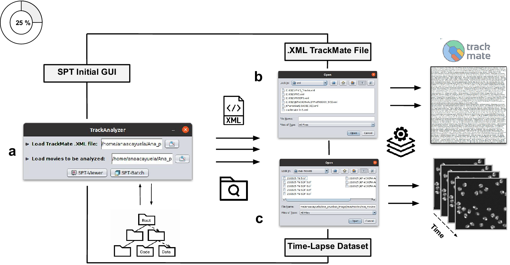
Figure 2. Illustration of getting started with the TrackAnalyzer plugin. (a) GUI structure of TrackAnalyzer. (b) TrackAnalyzer is started by selecting the .XML TrackMate configuration file and the time-lapse data sets to be analyzed in (c).
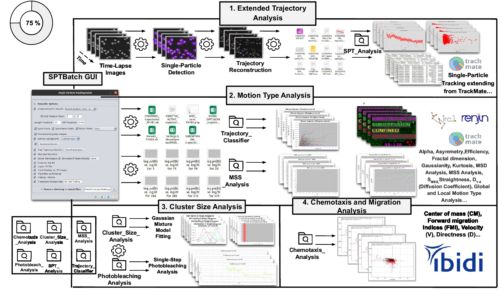
Figure 3. Schematic overview of the SPTBatch procedure for single-particle tracking along with subsequent motion trajectory analysis, cluster size, and single-step photobleaching analysis together with chemotaxis analysis in batch mode. (Reference Vera, Biswas, Senecal, Singer and Park1) Extended trajectory analysis. Single-particle tracking analysis extending from TrackMate running in batch mode using multiple sets of files. (Reference Cui, Yu, Yao, Xing, Lin and Li2) Motion Type Analysis. Trajectory analysis is executed to calculate short-time lag diffusion coefficient, diffusion coefficient, mean squared displacement curve, motion type classification, … (Reference Kok, Hebert and Huelsz-Prince3) Cluster size analysis and single-step photobleaching analysis is run. (Reference Hilsenbeck, Schwarzfischer and Skylaki4) Chemotaxis and migration analysis to quantify chemotactic cell migration.
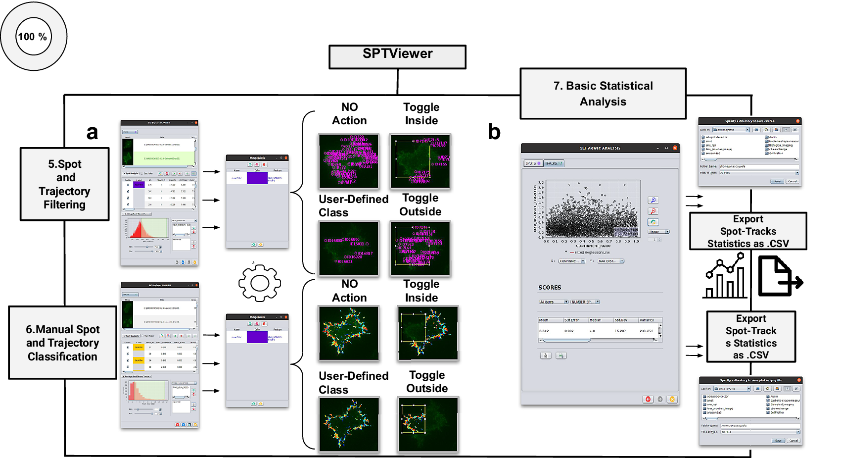
Figure 4. Schematic overview of the manual analysis for spot and trajectory filtering. (a) The double tabbed wizard-like GUI of our viewer in which the user can configure the settings for either spot or trajectory filtering along with user-definition of classes to identify specific spot or track types retaining. (b) SPTViewer last wizard enables to configure dynamic scatter plots to display any spot/track feature as a function of any other.
2.2. Validation of the method
2.2.1. Experimental dataset 1: Analysis of spot tracks
Analysis of the dynamic of CXCR4 at the plasma membrane of Jurkat CXCR4 $ {}^{-/-} $
cells electroporated with CXCR4-AcGFPm. In this example, we will illustrate the features that TrackAnalyzer offers for the different kinds of analysis of the tracks of spots. In particular, Steps 1, 2, and 3 (see Section 2.1 in Overview of the analysis procedure). Two datasets with Jurkat CXCR4
$ {}^{-/-} $
cells electroporated with CXCR4-AcGFPm. In this example, we will illustrate the features that TrackAnalyzer offers for the different kinds of analysis of the tracks of spots. In particular, Steps 1, 2, and 3 (see Section 2.1 in Overview of the analysis procedure). Two datasets with Jurkat CXCR4 $ {}^{-/-} $
cells electroporated with CXCR4-AcGFPm were used. This cell line, derived from human T lymphocytes, was generated using the CRISPR/Cas9 system to eliminate the endogenous expression of CXCR4(Reference García-Cuesta, Rodríguez-Frade and Gardeta
18
). Therefore, these cells only express CXCR4 labeled with AcGFPm. Cell sorting allowed us to obtain cells expressing 8,500 to 22,000 receptors per cell to work in single-particle conditions. It has been reported that ligand CXCL12 stimulation promotes CXCR4 nanoclustering at the cell membrane, which is necessary for a correct cell function(Reference Martínez-Muñoz, Rodríguez-Frade and Barroso
19
). In a previous work(Reference Martínez-Muñoz, Rodríguez-Frade and Barroso
19
), particles in TIRF images were automatically detected, tracked and analyzed using described algorithms for diffusion analysis(Reference Sorzano, Martínez-Muñoz, Cascio, García-Cuesta, Vargas, Mellado and Rodriguez Frade
20
) implemented in MATLAB. We now compare the results obtained in our previous work with TrackAnalyzer’s results.
$ {}^{-/-} $
cells electroporated with CXCR4-AcGFPm were used. This cell line, derived from human T lymphocytes, was generated using the CRISPR/Cas9 system to eliminate the endogenous expression of CXCR4(Reference García-Cuesta, Rodríguez-Frade and Gardeta
18
). Therefore, these cells only express CXCR4 labeled with AcGFPm. Cell sorting allowed us to obtain cells expressing 8,500 to 22,000 receptors per cell to work in single-particle conditions. It has been reported that ligand CXCL12 stimulation promotes CXCR4 nanoclustering at the cell membrane, which is necessary for a correct cell function(Reference Martínez-Muñoz, Rodríguez-Frade and Barroso
19
). In a previous work(Reference Martínez-Muñoz, Rodríguez-Frade and Barroso
19
), particles in TIRF images were automatically detected, tracked and analyzed using described algorithms for diffusion analysis(Reference Sorzano, Martínez-Muñoz, Cascio, García-Cuesta, Vargas, Mellado and Rodriguez Frade
20
) implemented in MATLAB. We now compare the results obtained in our previous work with TrackAnalyzer’s results.
The image sets studied in this case consist of time-lapse images acquired by a TIRF microscope (Leica AM TIRF inverted; 100x oil-immersion objective HCX PL APO 100x/1.46 NA) equipped with an EM-CCD camera (Andor DU 885-CS0–10-VP), at 37 °C with 5% CO2. Image sequences of individual particles (500 frames) were then acquired at 49% laser (488-nm diode laser) power with a frame rate of 10 Hz (100 ms per frame). The penetration depth of the evanescent field used was 90 nm. The first dataset contains image sequences from 18 different cells on fibronectin (basal) conditions (Figure 5a), while the second dataset contains image sequences from 14 different cells on fibronectin+CXCL12 (stimulated) conditions (Figure 5b).
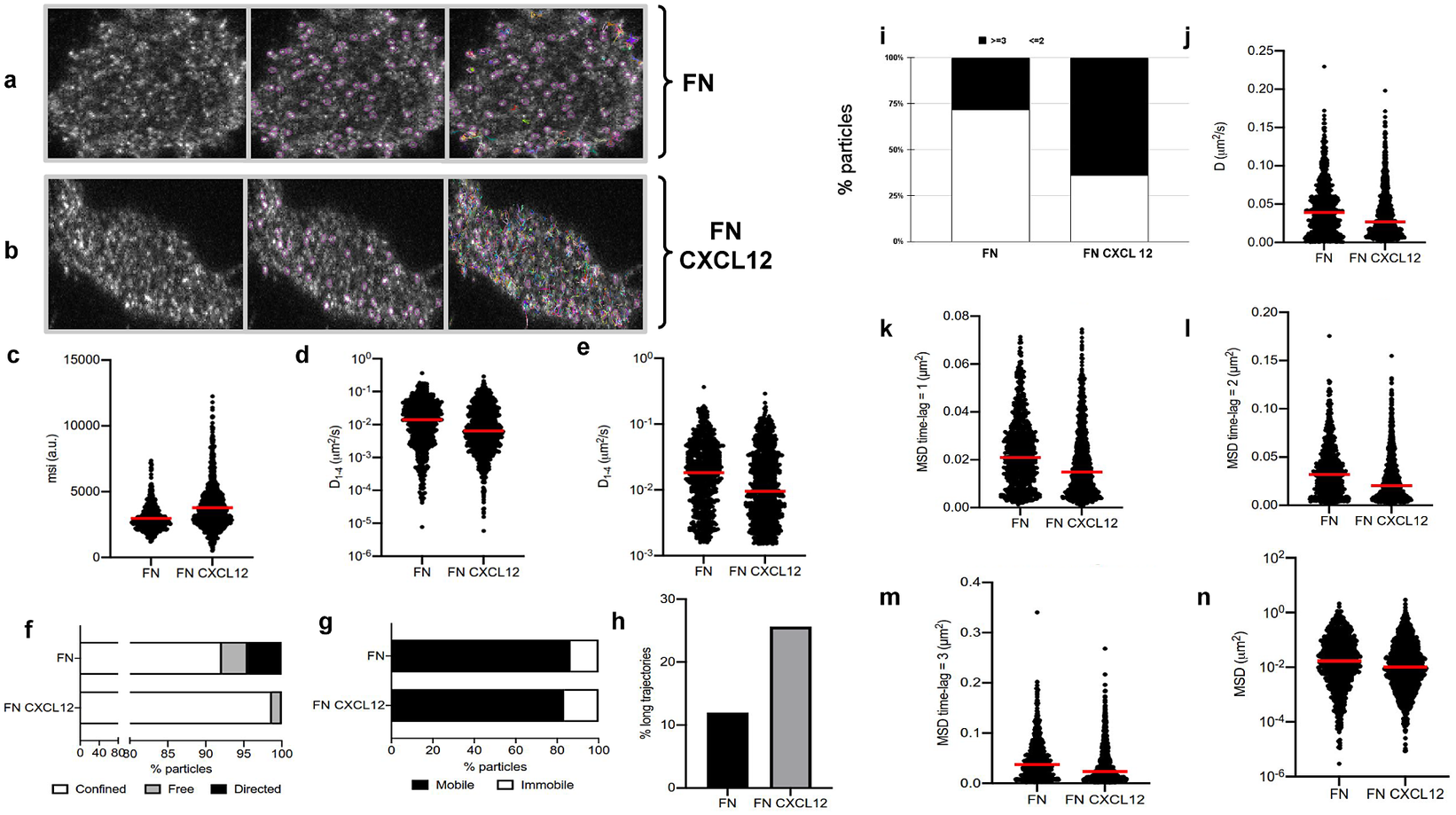
Figure 5. Application of TrackAnalyzer to track CXCR4-AcGFPm in JK CXCR4 $ {}^{-/-} $
cells electroporated with CXCR4-AcGFPm. (a-b) Images of Jurkat CXCR4
$ {}^{-/-} $
cells electroporated with CXCR4-AcGFPm. (a-b) Images of Jurkat CXCR4 $ {}^{-/-} $
cells electroporated with CXCR4-AcGFPm on fibronectin (FN)- (a) and FN + CXCL12-coated coverslips (b). Scale bar, 5 μm. (c–f) Tracking results from TrackAnalyzer (741 particles in 18 cells on FN and 1,209 particles in 14 cells on FN + CXCL12). (c) Mean spot intensity (MSI, arbitrary units, a.u.) from individual CXCR4-AcGFPm trajectories. The mean is indicated (red). Short-time lag diffusion coefficients (
$ {}^{-/-} $
cells electroporated with CXCR4-AcGFPm on fibronectin (FN)- (a) and FN + CXCL12-coated coverslips (b). Scale bar, 5 μm. (c–f) Tracking results from TrackAnalyzer (741 particles in 18 cells on FN and 1,209 particles in 14 cells on FN + CXCL12). (c) Mean spot intensity (MSI, arbitrary units, a.u.) from individual CXCR4-AcGFPm trajectories. The mean is indicated (red). Short-time lag diffusion coefficients ( $ {D}_{1-4} $
) of all (d) and mobile (e) single trajectories. The median is indicated (red). (***p
$ {D}_{1-4} $
) of all (d) and mobile (e) single trajectories. The median is indicated (red). (***p $ \le $
0.001, ****p
$ \le $
0.001, ****p $ \le $
0.0001, Welch’s t-test). (f) Percentage of confined, free and directed CXCR4-AcGFPm particles at the cell membrane using the slope of MSS. (g) Percentage of mobile and immobile CXCR4-AcGFPm particles at the cell membrane. (h) Percentage of long trajectories of CXCR4-AcGFPm particles at the cell membrane. (i) Frequency of CXCR4-AcGFP particles containing the same number of receptors [monomers plus dimers (Reference Cui, Yu, Yao, Xing, Lin and Li2)
$ \le $
0.0001, Welch’s t-test). (f) Percentage of confined, free and directed CXCR4-AcGFPm particles at the cell membrane using the slope of MSS. (g) Percentage of mobile and immobile CXCR4-AcGFPm particles at the cell membrane. (h) Percentage of long trajectories of CXCR4-AcGFPm particles at the cell membrane. (i) Frequency of CXCR4-AcGFP particles containing the same number of receptors [monomers plus dimers (Reference Cui, Yu, Yao, Xing, Lin and Li2) $ \le $
or nanoclusters (Reference Kok, Hebert and Huelsz-Prince3)
$ \le $
or nanoclusters (Reference Kok, Hebert and Huelsz-Prince3) $ \ge $
in cells, calculated from MSI values of each particle as compared with the MSI value of monomeric CD86-AcGFP. (j) Diffusion coefficients (D) of single trajectories. The median is indicated (red). (k) Mean Squared Displacement (MSD) of single trajectories using the first-time lag. The median is indicated (red). (l) Mean Squared Displacement (MSD) of single trajectories using the second time lag. The median is indicated (red). (m) Mean Squared Displacement (MSD) of single trajectories using third time-lag. The median is indicated (red). (n) Mean Squared Displacement (MSD) of single trajectories using more than three time-lags. The median is indicated (red).
$ \ge $
in cells, calculated from MSI values of each particle as compared with the MSI value of monomeric CD86-AcGFP. (j) Diffusion coefficients (D) of single trajectories. The median is indicated (red). (k) Mean Squared Displacement (MSD) of single trajectories using the first-time lag. The median is indicated (red). (l) Mean Squared Displacement (MSD) of single trajectories using the second time lag. The median is indicated (red). (m) Mean Squared Displacement (MSD) of single trajectories using third time-lag. The median is indicated (red). (n) Mean Squared Displacement (MSD) of single trajectories using more than three time-lags. The median is indicated (red).
Before entering into TrackAnalyzer, we generated an XML parameter file with TrackMate. Spots were identified through subpixel localization applying Laplacian of Gaussian (LoG) detector(Reference Tinevez, Perry and Schindelin 12 ) (estimated object diameter = 0.5 μm, quality threshold = 500, Sub-pixel localization = true, Median filtering = true). Frame-to-frame spot linking was performed using TrackMate’s linear assignment problem (LAP) by closing gaps (linking max distance = 0.5 μm; track segment gap closing = 0.1 μm and 6 frames; track filtering of those trajectories of at least 20 frames).
We then launched TrackAnalyzer in batch mode to analyze all videos in the datasets with the same parameters. The following paragraphs provide the parameters and describe the results of the different kinds of analyses.
-
1. Extended trajectory analysis. We did not discard any of the identified tracks. As can be seen in Figure 5c, stimulation with CXCL12 promotes an increase in the mean spot intensities (MSI) mean value of CXCR4 particles (2,970 arbitrary units for fibronectin versus 3,781 arbitrary units for fibronectin+CXCL12) reflecting an increase of larger CXCR4 nanoclusters.
-
2. Motion-type analysis. A diffusion coefficient of 0.0015 was set as the threshold to discriminate among mobile and immobile particles, which is the percentile 95 of the diffusion coefficients of purified AcGFPm protein particles immobilized on glass coverslips(Reference Martínez-Muñoz, Rodríguez-Frade and Barroso 19 ). Figure 5d,e,g,j–n show the
$ {D}_{1-4} $
, D, MSD, and percentage of the immobile particles. There is an increase in the percentage of immobile particles in CXCL12-stimulated conditions (6.12% for fibronectin vs 10.40% for fibronectin+CXCL12). Mobile particles also showed a reduction in the MSD and
$ {D}_{1-4} $
demonstrating a significant reduction in overall receptor diffusivity (0,012 μm2/s for fibronectin vs 0,007 μm2/s for fibronectin+CXCL12). These results are consistent with those previously obtained using Matlab(Reference García-Cuesta, Rodríguez-Frade and Gardeta
18
, Reference Martínez-Muñoz, Rodríguez-Frade and Barroso
19
), in which CXCL12 stimulation promoted the formation of larger nanoclusters of CXCR4 that also showed a different dynamic behavior as compared with the receptor in basal conditions.


We classified the trajectories whose length is larger than 50 frames into confined, anomalous, Brownian (free), or directed (Figure 5f) using the MSS described in Section 5.1 along with the percentage of long trajectories per condition.
3. Cluster size analysis. We used the background subtraction method 4 (described in Section 5.2). The total number of receptors per particle was assessed by dividing the mean particle intensity by the particle arising from monomeric protein, that is CD86-AcGFP, estimated through the analysis of spots with just one photobleaching step. Therefore, this value was used as the monomer reference to estimate the number of receptors or molecules per particle, as shown in Figure 5i.
2.2.2. Experimental dataset 2: Analysis of cell tracks
Analysis of the directed cell migration capacity of Jurkat cells. In this section, we illustrate the chemotaxis and migration analysis module. To do so, we only use Steps 1 and 4 (see Section 2.1 in Overview of the analysis procedure). Note that some of the steps only apply to spots and not cells, for instance, Steps 2 and 3.
4. Chemotaxis and migration analysis. In this analysis, we will illustrate other features of TrackAnalyzer to evaluate directional cell migration. Two datasets with Jurkat cells were used. To assess the ability of these cells, which express CXCR4 endogenously, to migrate toward CXCL12 gradients, we used fibronectin-coated chemotaxis chambers (Ibidi μ Slide Chemotaxis System; 80326). As CXCL12 is the ligand of CXCR4, we expected that cells migrate toward the gradient. The image sets studied in this case consist of time-lapse images acquired by a Microfluor inverted microscope (Leica) every 2 min for 6 h at 37 °C with $ 5\% $
CO2. Single-cell tracking analysis was performed using TrackMate to generate an XML parameter file. Cells were identified through subpixel localization by applying LoG detector (estimated object diameter = 0.5 μm, quality threshold = 15.0, Sub-pixel localization = true, Median filtering = true). Frame-to-frame cell linking was performed using TrackMate’s LAP by closing gaps (linking max distance = 60 μm; track segment gap closing = 60 μm and 2 frames). Then we launched TrackAnalyzer to analyze all videos in the datasets with these parameters. Therefore, directional cell migration was assessed (Figure 6) by evaluating the corresponding spider plots (representing the trajectories of the tracked cells) (Figure 6a,b), forward migration index (FMI) (Figure 6e), directionality (D) (Figure 6f), the CM (Figure 6d) and velocity (V) (Figure 6c) provided by chemotaxis and migration plugin integration. Quantitation of the results showed that JK cells sensed the CXCL12 gradient to increase the FMI, directionality, CM and velocity.
$ 5\% $
CO2. Single-cell tracking analysis was performed using TrackMate to generate an XML parameter file. Cells were identified through subpixel localization by applying LoG detector (estimated object diameter = 0.5 μm, quality threshold = 15.0, Sub-pixel localization = true, Median filtering = true). Frame-to-frame cell linking was performed using TrackMate’s LAP by closing gaps (linking max distance = 60 μm; track segment gap closing = 60 μm and 2 frames). Then we launched TrackAnalyzer to analyze all videos in the datasets with these parameters. Therefore, directional cell migration was assessed (Figure 6) by evaluating the corresponding spider plots (representing the trajectories of the tracked cells) (Figure 6a,b), forward migration index (FMI) (Figure 6e), directionality (D) (Figure 6f), the CM (Figure 6d) and velocity (V) (Figure 6c) provided by chemotaxis and migration plugin integration. Quantitation of the results showed that JK cells sensed the CXCL12 gradient to increase the FMI, directionality, CM and velocity.
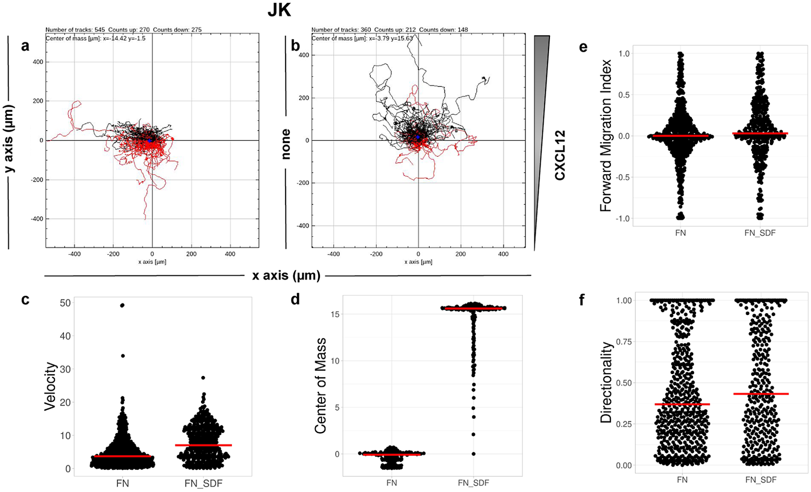
Figure 6. Migration of JK cells in response to a CXCL12 gradient. (a,b) Representative spider plots showing the trajectories of tracked cells migrating along the gradient (black) or moving in the opposite direction (red). Black and red dots in the plots represent the final position of each single-tracked cell. The grey triangle indicates CXCL12 gradient. Quantification of the velocity (c), center of mass (d), forward migration index (e), and directionality (f) of experiments performed.
Note that Steps 5, 6, and 7 are not presented in this section because its applicability does not address the biological questions arising from this context. Rather, they are deeply described in detail in Section 2.1 in Overview of the analysis procedure.
3. Discussion
TrackAnalyzer extends the existing tools for single-particle tracking analysis in two ways:
-
1. Batch-mode analysis. Most existing tools in ImageJ and Fiji allow the analysis of a single time-lapse dataset. However, many users and facilities do not have a single dataset but many datasets to analyze. Our tool allows the automatic analysis of all of them by configuring the analysis in one of them and replicating the same analysis to all other videos within the same experiment relying on the graphical user interface (GUI).
-
2. Extended analysis. Most existing tools in ImageJ and Fiji specialize in a particular aspect of the tracks, for instance: TrackMate in identifying the spots and linking them into tracks; TraJClassifier in identifying their motion; Chemotaxis and Migration Tool in analyzing their motion from a different perspective. However, the user is also interested in other features like cluster size, measuring the motion in multiple ways, classifying the tracks into different categories and comparing their different features as a function of their categories, and removing from the analysis those tracks that have been incorrectly identified or focusing the analysis in a particular region of the cell. Our tool builds upon existing powerful tools and adds newly implemented measures to allow a more thorough analysis of all the tracks recorded in an experiment. In this way, we allow a very rich analysis of the particles’ behavior under various experimental conditions and allow a quantitative comparison of the different parameters that characterize the particles.
A track analysis’s strength is correctly identifying the spots and their linkage to tracks. This is a rather challenging task that, if performed incorrectly, totally ruins the automatic analysis. TrackMate is extremely flexible in this aspect. It provides many different algorithms for spot identification, all of them fully configurable through a myriad of parameters (although the default values of most of them already give good results). TrackMate is also very strong and flexible in constructing the tracks from the set of spots. It also offers several highly configurable algorithms. In this regard, we consider that a semiautomated approach in which the user makes sure to configure the spot and track detection for his/her experimental conditions is crucial. This step is the key to the success of all the subsequent analyses. We have decided to rely on TrackMate for this identification step, as it is one of the most successful and adaptable programs available.
Icy(Reference de Chaumont, Dallongeville and Chenouard 21 ) could have been an alternative to TrackMate. Icy is a free and open-source software for image analysis mainly oriented toward analyzing biological images with a modular design composed of a kernel and plugins. Icy software integrates the Spot Tracking plugin(Reference Chenouard, Bloch and Marin 22 ), which ships automated methods for extracting tracks (particle tracking) from multiple objects (particle detection) as well as the Track Manager plugin which provides relevant information from them (track analysis) in a sequence of 2D or 3D images. Track Manager allows the use of DSP-like trackProcessors enabling the display of tracks, time-based or ROI-based selection, and the generation of various views such as overlaid and animated local flow and polar graphs. These tools afford track filtering, classification (split tracks into tracklets to further statistically classify as Brownian/confined or directed), characterization by extracting features (confinement ratio, displacement distance, lifetime, intensity profile, instant speed, MSD, interaction analysis among tracked objects…) together with post-processing (export tracks into CSV files). This is a powerful tool to accurately perform common SPT analyses but compared with the integration of TraJClassifier, Icy may lack advanced track analysis capabilities. TraJClassifer provides diffusion characterization through the TraJ library and subsequent track classification by using simulated tracks of ND, subdiffusion, CD and DM. Then a group of features is estimated for each track, which together with the corresponding class, are used to train a random forest approach by means of Renjin. This extended track analysis also supports local analysis by splitting the track into single segments with different motion types.
TrackAnalyzer benefits from the ImageJ ecosystem, probably the most known, flexible, and longest-lived software for biomedical sciences. Consequently, TrackAnalyzer leverages a lot of plugins for scientific image processing (as we have already done by integrating TrackMate with TraJClassifier and the Chemotaxis and Migration tool). To the best of our knowledge, TrackAnalyzer is the first tracking program within ImageJ that enables users to characterize and classify trajectories by a large number of descriptors, including the intensity and length of the tracks, multiple characterizations of their motion, cluster size by various methods, and their chemotactic features. Some protocols to quantitatively assess the tracks’ motion, cluster size, and intensity analysis were already designed in our previous work(Reference Sorzano, Martínez-Muñoz, Cascio, García-Cuesta, Vargas, Mellado and Rodriguez Frade 20 ). However, TrackAnalyzer now largely supersedes our analysis capacity.
4. Conclusions
In this paper, we have introduced TrackAnalyzer, a new Java-based plugin, an open-source and user-friendly toolkit to perform SPT analysis of multidimensional data in batch mode. This plugin operates equally well under ImageJ or Fiji ecosystems extending from TrackMate algorithms for (I) spot detection and spot analysis in which each spot receives a wide range of features based on its location, radius, and metadata information; (II) linking spots together to build trajectories and get the subsequent trajectory analysis; (III) post-processing actions after SPT analysis such as 2D visualization and user-defined filtering of spots and trajectories. Our approach is semiautomatic as the user needs to define the TrackMate workflow to identify the spots. This strategy makes us capable of dealing with challenging experimental scenarios such as low signal-to-noise ratios or strong fluorescence backgrounds. In addition to the standard track analysis offered by TrackMate, we have included multiple ways of filtering the detected spots and tracks and various characterizations of their motion type, cluster size, chemotaxis, and migration properties.
5. Materials and Methods
5.1. Motion analysis
Calculation of Mean Squared Displacement (MSD)
The MSD is the most common approach for analyzing single-particle tracks(Reference Manzo and Garcia-Parajo
5
). Let us call $ \Delta t $
to the time difference between one frame in the time-lapse video and the next. The MSD of the particle
$ \Delta t $
to the time difference between one frame in the time-lapse video and the next. The MSD of the particle $ j $
with time lag
$ j $
with time lag $ n\Delta t $
is defined as follows(Reference Wagner, Kroll, Haramagatti, Lipinski and Wiemann
13
):
$ n\Delta t $
is defined as follows(Reference Wagner, Kroll, Haramagatti, Lipinski and Wiemann
13
):
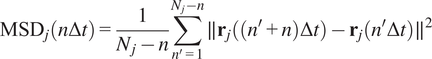 $$ {\mathrm{MSD}}_j\left(n\Delta t\right)=\frac{1}{N_j-n}\sum \limits_{n^{\prime }=1}^{N_j-n}\parallel {\mathbf{r}}_j\left(\left({n}^{\prime }+n\right)\Delta t\right)-{\mathbf{r}}_j\left({n}^{\prime}\Delta t\right){\parallel}^2 $$
where $ {\mathbf{r}}_j\left({n}^{\prime}\Delta t\right) $
is the 2D location of the
$ {\mathbf{r}}_j\left({n}^{\prime}\Delta t\right) $
is the 2D location of the $ j $
th particle at time
$ j $
th particle at time $ {n}^{\prime}\Delta t $
, and
$ {n}^{\prime}\Delta t $
, and $ {N}_j $
is the length of the
$ {N}_j $
is the length of the $ j $
-th trajectory in frames.
$ j $
-th trajectory in frames.
Calculation of Diffusion Coefficient ( $ D $
)
$ D $
)
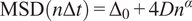
The diffusion coefficient ( $ D $
) is defined as the slope of the linear fitting of the first time lag of the MSD curve:
$ D $
) is defined as the slope of the linear fitting of the first time lag of the MSD curve:
 $$ \mathrm{MSD}\left(n\Delta t\right)={\Delta}_0+4 Dn\hskip1em n=1 $$
Calculation of the Short-Time Lag Diffusion Coefficient ( $ {D}_{1-N} $
)
$ {D}_{1-N} $
)
The short-time lag diffusion coefficients ( $ {D}_{1-N} $
) are defined as the slope of the linear fitting of the first N time lags (defined by the user) of the MSD curve:
$ {D}_{1-N} $
) are defined as the slope of the linear fitting of the first N time lags (defined by the user) of the MSD curve:
 $$ \mathrm{MSD}\left(n\Delta t\right)={\Delta}_0+4{D}_{1-N}n\hskip1em n=1,2,\dots N-1 $$
Calculation of the Anomalous Exponent ( $ \alpha $
)
$ \alpha $
)
The MSD plots must be fitted according to the AD model by power law fitting(Reference Manzo and Garcia-Parajo 5 ) according to the following equation:
 $$ \mathrm{MSD}\left(n\Delta t\right)={\Delta}_0+4{Dn}^{\alpha } $$
being $ \alpha $
the anomalous exponent. The particle motion-type is classified as confined (0 <
$ \alpha $
the anomalous exponent. The particle motion-type is classified as confined (0 < $ \alpha $
< 0.6), Brownian or free (0.9 <
$ \alpha $
< 0.6), Brownian or free (0.9 < $ \alpha $
< 1.1) or directed (
$ \alpha $
< 1.1) or directed ( $ \alpha $
> 1.1)(Reference Manzo and Garcia-Parajo
5
).
$ \alpha $
> 1.1)(Reference Manzo and Garcia-Parajo
5
).
5.1.1.
Calculation of moment scaling spectrum (MSS) and its slope,
$ \left({S}_{\mathrm{MSS}}\right) $

In the case of long trajectories, theMSS(Reference Ferrari, Manfroi and Young
15
, Reference Arts, Smal, Paul, Wyman and Meijering
23
, Reference Vega, Freeman, Grinstein and Jaqaman
24
) and its slope $ \left({S}_{\mathrm{MSS}}\right) $
were proposed as an approach to improve the calculation of MSD for nonlinear diffusion. For each trajectory
$ \left({S}_{\mathrm{MSS}}\right) $
were proposed as an approach to improve the calculation of MSD for nonlinear diffusion. For each trajectory $ j $
the moments of displacement
$ j $
the moments of displacement $ \left({\mu}_{j,\nu}\right) $
were calculated for
$ \left({\mu}_{j,\nu}\right) $
were calculated for $ \nu =1,\dots, 6 $
as a function of time according to the following equation:
$ \nu =1,\dots, 6 $
as a function of time according to the following equation:
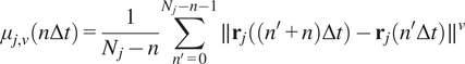 $$ {\mu}_{j,\nu}\left(n\Delta t\right)=\frac{1}{N_j-n}\sum \limits_{n^{\prime }=0}^{N_j-n-1}\parallel {\mathbf{r}}_j\left(\left({n}^{\prime }+n\right)\Delta t\right)-{\mathbf{r}}_j\left({n}^{\prime}\Delta t\right){\parallel}^{\nu } $$
where $ {r}_j $
designates the position vector of track
$ {r}_j $
designates the position vector of track $ j $
at the time
$ j $
at the time $ n\Delta t $
being
$ n\Delta t $
being $ \Delta t $
the time interval and
$ \Delta t $
the time interval and $ n $
the frame number
$ n $
the frame number $ n=0,1,\dots {N}_j-1 $
being
$ n=0,1,\dots {N}_j-1 $
being $ {N}_j $
the trajectory length. The MSD is just a special case with
$ {N}_j $
the trajectory length. The MSD is just a special case with $ \nu =2 $
. In our implementation, we calculate all moments from
$ \nu =2 $
. In our implementation, we calculate all moments from $ \nu =1 $
to
$ \nu =1 $
to $ \nu =6 $
for each trajectory by plotting
$ \nu =6 $
for each trajectory by plotting $ \left({\mu}_{j,\nu}\right) $
against
$ \left({\mu}_{j,\nu}\right) $
against $ n\Delta t $
in a double logarithmic plot, getting the scaling moments
$ n\Delta t $
in a double logarithmic plot, getting the scaling moments $ {\gamma}_{j,\nu } $
from assuming each moment
$ {\gamma}_{j,\nu } $
from assuming each moment $ \mu $
depends on the time shift according to
$ \mu $
depends on the time shift according to $ {\mu}_{\nu}\left(n\Delta \right)\sim n\Delta {t}^{\gamma \mu} $
(Reference Ewers, Smith, Sbalzarini, Lilie, Koumoutsakos and Helenius
14
, Reference Ferrari, Manfroi and Young
15
). Therefore plotting
$ {\mu}_{\nu}\left(n\Delta \right)\sim n\Delta {t}^{\gamma \mu} $
(Reference Ewers, Smith, Sbalzarini, Lilie, Koumoutsakos and Helenius
14
, Reference Ferrari, Manfroi and Young
15
). Therefore plotting $ {\gamma}_{\nu } $
against
$ {\gamma}_{\nu } $
against $ \nu $
gives the MSS and its slope (
$ \nu $
gives the MSS and its slope ( $ {S}_{\mathrm{MSS}} $
) from linear regression characterizes the type of motion(Reference Siebrasse, Djuric and Schulze
25
): free (
$ {S}_{\mathrm{MSS}} $
) from linear regression characterizes the type of motion(Reference Siebrasse, Djuric and Schulze
25
): free ( $ {S}_{\mathrm{MSS}} $
= 0.5), directed (
$ {S}_{\mathrm{MSS}} $
= 0.5), directed ( $ {S}_{\mathrm{MSS}} $
> 0.5), immobile (
$ {S}_{\mathrm{MSS}} $
> 0.5), immobile ( $ {S}_{\mathrm{MSS}} $
< 0.5).
$ {S}_{\mathrm{MSS}} $
< 0.5).
5.1.2.
Calculation of forward migration index
$ \left({\mathrm{FMI}}^{\parallel },{\mathrm{FMI}}^{\perp}\right) $

The FMIis an important measure for directed, chemotactic cell migration. It represents the efficiency of the forward migration of cells in the direction of a chemical gradient, $ \mathbf{u} $
. We assume that
$ \mathbf{u} $
. We assume that $ \mathbf{u} $
has unit length, and we also consider a direction perpendicular to
$ \mathbf{u} $
has unit length, and we also consider a direction perpendicular to $ \mathbf{u} $
that will be referred to as
$ \mathbf{u} $
that will be referred to as $ {\mathbf{u}}^{\perp } $
. For a given particle,
$ {\mathbf{u}}^{\perp } $
. For a given particle, $ j $
, let
$ j $
, let $ {\mathbf{r}}_j(0) $
and
$ {\mathbf{r}}_j(0) $
and $ {\mathbf{r}}_j\left({N}_j\Delta t\right) $
be the first and last locations of its trajectory. The efficiency of the displacement in both directions are as follows:
$ {\mathbf{r}}_j\left({N}_j\Delta t\right) $
be the first and last locations of its trajectory. The efficiency of the displacement in both directions are as follows:
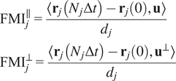 $$ {\displaystyle \begin{array}{l}{\mathrm{FMI}}_j^{\parallel }=\frac{\left\langle {\mathbf{r}}_j\left({N}_j\Delta t\right)-{\mathbf{r}}_j(0),\mathbf{u}\right\rangle }{d_j}\\ {}{\mathrm{FMI}}_j^{\perp }=\frac{\left\langle {\mathbf{r}}_j\left({N}_j\Delta t\right)-{\mathbf{r}}_j(0),{\mathbf{u}}^{\perp}\right\rangle }{d_j}\end{array}} $$
where $ \left\langle \cdot, \cdot \right\rangle $
denotes the inner product, and
$ \left\langle \cdot, \cdot \right\rangle $
denotes the inner product, and $ {d}_j $
is the total length of the
$ {d}_j $
is the total length of the $ j $
-th trajectory. The FMIs must be between −1 and 1. The larger the FMI in absolute value, the stronger the chemotactic effect is on the direction being studied. Finally, for a whole video, the FMI in a particular direction, parallel or perpendicular, is defined as the average of the corresponding particle FMIs.
$ j $
-th trajectory. The FMIs must be between −1 and 1. The larger the FMI in absolute value, the stronger the chemotactic effect is on the direction being studied. Finally, for a whole video, the FMI in a particular direction, parallel or perpendicular, is defined as the average of the corresponding particle FMIs.
5.1.3. End center of mass (
$ {\mathbf{r}}_{end} $
)

The CM represents the average of all single-cell endpoints. Its $ x $
and
$ x $
and $ y $
values indicate the direction in which the group of cells primarily travelled.
$ y $
values indicate the direction in which the group of cells primarily travelled.
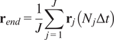 $$ {\mathbf{r}}_{end}=\frac{1}{J}\sum \limits_{j=1}^J{\mathbf{r}}_j\left({N}_j\Delta t\right) $$
where $ J $
is the total number of cells and
$ J $
is the total number of cells and $ {\mathbf{r}}_j\left({N}_j\Delta t\right) $
are the coordinates of the endpoint of each cell.
$ {\mathbf{r}}_j\left({N}_j\Delta t\right) $
are the coordinates of the endpoint of each cell.
5.1.4. Directness (
$ D $
)

The directness or directionality measures the straightness of the cell trajectories. For each cell, it is calculated by comparing the Euclidean distance and the accumulated distance between the starting point and the endpoint of a migrating cell:
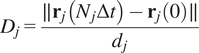 $$ {D}_j=\frac{\parallel {\mathbf{r}}_j\left({N}_j\Delta t\right)-{\mathbf{r}}_j(0)\parallel }{d_j} $$
The directness values are always positive. A directness of $ D=1 $
equals a straight-line migration from the start to the endpoint. The directness of a video is the average of the directness of all its cells.
$ D=1 $
equals a straight-line migration from the start to the endpoint. The directness of a video is the average of the directness of all its cells.
5.2. Estimation of the background fluorescence
We now describe the different methods that we propose to estimate the background fluorescence.
-
• Subtract Bg 1 (manual). Manual identification for each frame. This method enables user to manually select an indefinite number of positions over the Z-Projection image to ensure that the mean intensity measured belongs exclusively to areas within cell outside spots. This approach measures the mean background intensity for each frame for all selected locations along the video.
-
• Subtract Bg 2 (spot ring). This approach estimates the mean background intensity of each spot. It measures the intensity in a ring ranging from its radius to twice its radius.
-
• Subtract Bg 3 (inside the cell, not excluding spots). This approach measures the mean background intensity for each frame by identifying the cell in each frame based. Then, the background mean intensity value is computed as the average within these masks (not excluding spots).
-
• Subtract Bg 4 (inside the cell excluding spots). This approach measures the mean background intensity for each frame by identifying the cell in each frame based. The background is estimated as the average intensity within the cell, excluding the spot positions.
-
• Subtract Bg 5 (rolling ball). This method estimates a locally varying background as the average within a rolling ball(Reference Sternberg 26 ). It is important to note that the ball radius must be larger than the radius of the largest spot in the image.
5.3. Development and Implementation
TrackAnalyzer was developed in the Eclipse Integrated Development Environment (IDE)(Reference desRivieres and Wiegand 27 ) for Java Developers version 2019–12 (4.14.0), an open-source platform mainly written in Java and used in computer programming for computer programming developing user-friendly Java applications. Each plugin is a Java application that inherits from ImageJ’s plugin class extending from the TrackMate ecosystem. The core software and GUI were built using Java 8. Plots and histograms were implemented using the JFreeChart library. For reading the input images, we used the Bio-formats library(Reference Linkert, Rueden and Allan 28 ). For handling XML files, we used JDom, and for taking Microsoft Office Formats (.xls,.xlsx), we used Apache POI libraries. In the case of classifying trajectories, we called the TraJ Java library for diffusion trajectory (2D) analysis.
The source code and documentation are available at https://github.com/QuantitativeImageAnalysisUnitCNB/TrackAnalyzer_.
5.4. Installation in Fiji or ImageJ
TrackAnalyzer must be installed as a plugin of Fiji or ImageJ (https://imagej.nih.gov/ij/download.html) and consequently can be executed in Windows, Mac OS, or Linux systems. The next step is to install TrackAnalyzer, which can be done by downloading the plugin from http://sites.imagej.net/TrackAnalyzer/plugins/ and moving into the ImageJ/Fiji plugins subfolder. Alternatively, it can be dragged and dropped into the ImageJ/Fiji main window or installed through the ImageJ/Fiji menu bar Plugins → Install → Path to File. After installing the plugin, ImageJ or Fiji must be restarted. Note that to visualize the wizard-like GUI that guides the user through the set of predefined steps in this plugin, the user must navigate to TrackAnalyzer_Additional_Files, download from plugins folder the JWizardComponent_.jar, and locate it into the ImageJ/Fiji plugins subfolder. Moreover, to avoid any bugs while running the TraJClassifier motion classification routine, the user must download the .jar files from jars folder the .jar files and move them into the ImageJ/Fiji jars subfolder. For those users using Fiji, all steps described above can be skipped, the TrackAnalyzer update site can be followed according to the instructions at https://imagej.net/Following_an_update_site.
5.5. Supported image file formats
Our plugin deals with a wide range of file formats using Bio-Formats(Reference Linkert, Rueden and Allan 28 ), an open-source library from life sciences supporting or reading almost any image format or multidimensional data as z-stacks, time series, or multiplexed images keeping metadata easily accessible. On top of that, the user can access a list of time-lapse images available during the whole procedure to update the analysis as often as needed.
Acknowledgments
We are very grateful to members of the Department of Immunology and Oncology at the National Center for Biotechnology for providing us with the time-lapse datasets and their collaborative help in this research.
Competing interest
The authors declare none.
Authorship contribution
A.C.L., J.A.G-P., and C.O.S.S. conceived the project and designed the algorithms. A.C.L. wrote the software code and performed all experiments. E.M.G-C. prepared the samples and acquired the images at the microscope. All authors wrote and revised the manuscript.
Funding statement
This research was supported by the Spanish MICINN (PRE2018–086112) by the FPI fellowship from the Spanish Ministry of Science and Innovation through the Severo Ochoa excellence accreditation SEV-2017-0712-18-1. Also, we would like to acknowledge economic support from Grant PID2019-104757RB-I00 funded by MCIN/AEI/ 10.13039/501100011033/ and “ERDF A way of making Europe”, by the “European Union”, SEV-2017-0712 funded by MCIN/AEI/10.13039/501100011033, European Union (EU) and Horizon 2020 through grant HighResCells (ERC - 2018 - SyG, Proposal: 810057).
Data availability statement
The source code and documentation for the plugin are available at https://github.com/QuantitativeImageAnalysisUnitCNB/TrackAnalyzer_.


 Open access