


Impact Statement
The advent of spatially resolved transcriptomics (SRT) technologies has facilitated the study of gene expression in an anatomical context. However, next-generation sequencing (NGS)-based SRT approaches pose an emerging challenge: integrating transcriptome-wide spatial gene expression with high-resolution tissue images (brightfield histology or fluorescent antibody staining) to generate precise maps of spatial gene expression across intact tissue sections. We developed VistoSeg as an image-processing software to address these needs. VistoSeg is currently compatible with the Visium and Visium Spatial Proteogenomics (Visium-SPG) platforms (10× Genomics), which are NGS-based SRT assays employing histological and immunofluorescent tissue images, respectively. VistoSeg provides computational imaging-processing tools to extract cell number, cell type identity, and other image-derived metrics at spatially defined locations across the tissue section to incorporate with corresponding gene expression measurements.
1. Introduction
In the past decade, RNA sequencing (RNA-seq) moved beyond profiling in homogenate tissue to defining gene expression at single-cell or single-nucleus (sc/snRNA-seq) resolution. This technological development motivated the generation of new computational methods that answered many previously unaddressed biological questions. However, spatial information about where cells resided within the tissue remained lacking. Spatially resolved transcriptomics (SRT) is a new class of technologies that measures gene expression along spatial coordinates.(Reference Marx1) Next-generation sequencing (NGS)-based SRT technologies are especially powerful for their ability to define transcriptome-wide gene expression patterns across intact tissue sections. While there are several laboratories that have developed custom methods to perform NGS-based SRT,(Reference Rodriques, Stickels, Goeva, Martin, Murray, Vanderburg, Welch, Chen, Chen and Macosko2–Reference Fu, Sun, Chen, Dong, Lin, Palmiter, Lin and Gu5) the commercially available Visium platform from 10× Genomics is the leading and most widely adopted technology for generating transcriptome-wide spatial gene expression data in intact tissue sections.(Reference Moses and Pachter6) Because SRT data includes paired gene expression and microscopy images from the same tissue section, analysis of this data necessitates tools to integrate both modalities.
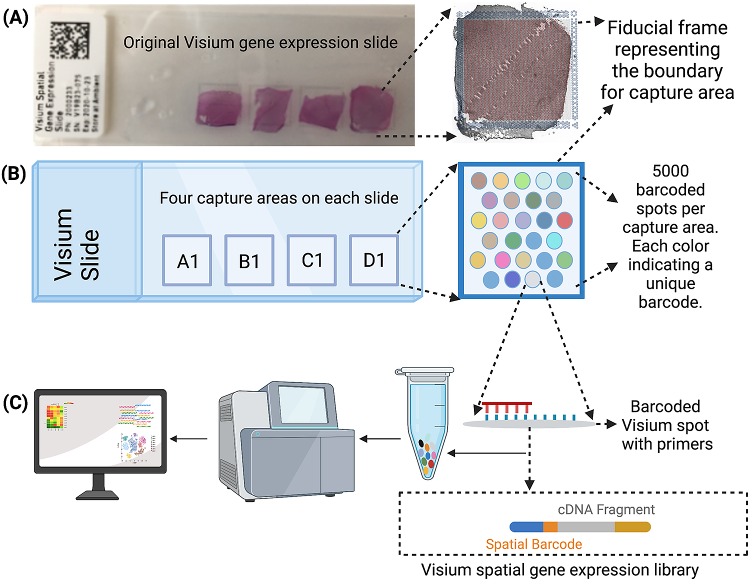
The Visium workflow uses an on-slide spatial barcoding strategy to map RNA-seq reads to defined anatomical locations (“spots”) in an intact tissue section (Figure 1a). Briefly, each slide contains four arrays (Figure 1b: A1, B1, C1, D1), and each array contains ~5,000 gene expression capture “spots,” which are 55 μm in diameter (2,375 μm2 in area) and spaced 100 μm center-to-center in a honeycomb pattern (Figure 1b). On-slide cDNA synthesis incorporates spatial barcodes for each spot, which is followed by RNA-seq to obtain gene expression measurements at each anatomical location (Figure 1c). The platform currently supports two major workflows: Visium-H&E and Visium-Spatial Proteogenomics (Visium-SPG). In the Visium-H&E workflow, tissue sections are stained with hematoxylin and eosin (H&E), and a brightfield histological image is acquired. In Visium-SPG, tissue sections are labeled with antibodies conjugated to fluorophores, and multiplex fluorescent images are acquired to visualize specific proteins of interest. In both cases, images are used to create an integrated map of transcriptome-wide gene expression within the tissue architecture. In the case of Visium-SPG, transcriptomic data can also be analyzed in the context of proteomic data from antibody labeling.
Visium workflow. (a) Visium spatial gene expression slide containing four 6.5 mm x 6.5 mm capture areas bound by a fiducial frame. (b) Each capture area contains a grid printed with ~5,000 spots with unique spatial barcodes that allow mRNA measurements to be mapped back to the X–Y location on the tissue. (c) Spatial barcodes are incorporated during on-slide cDNA synthesis. The cDNA is eluted off the slide, and libraries are prepared and sequenced. Reads are mapped to spatial coordinates on the histological image using SpaceRanger software (10× Genomics), which provides a transcriptome-wide readout of gene expression at each spatial coordinate.
To maintain RNA integrity for compatibility with downstream transcriptomic workflows, speed and throughput capacity are important considerations for image acquisition protocols. In line with these considerations, imaging is often performed on slide scanners or other high-throughput microscopy systems that are commonly used for pathology image acquisition and analysis. To support integration with downstream molecular gene expression data, preprocessing utilities are needed to separate the large whole-slide images into single images representing each individual tissue section. These images then need to be further segmented to extract meaningful metrics about cell number, morphology, position, etc. Current analytical tools available from 10× Genomics focus heavily on gene expression data and do not support in-depth processing or analysis (e.g., nuclear or cellular segmentation) of imaging data. Specifically, 10× Genomics provides two software programs, Loupe Browser(7) and SpaceRanger,(8) which enable data extraction and primary visualization of SRT data, but have limited functionality for more advanced processing.
Other existing software also fail to provide the necessary functionalities that would allow users to take the images from preprocessing to quantitative integration of gene expression data with extracted metrics. For example, the open source software package QuPath(Reference Bankhead, Loughrey, Fernández, Dombrowski, McArt, Dunne, McQuaid, Gray, Murray, Coleman, James, Salto-Tellez and Hamilton9) does not support preprocessing of the multichannel fluorescent images and requires downsampling, resulting in reduced image resolution when opening, cropping and exporting images. The commercially available image analysis software HALO enables quantification and classification of cells and nuclei, but does not support integration with gene expression data. Several software packages have been developed in the Python and R programming languages for cell segmentation and subsequent registration of microscopy images to anatomical reference atlases.(Reference Stringer, Wang, Michaelos and Pachitariu10, Reference Fürth, Vaissière, Tzortzi, Xuan, Märtin, Lazaridis, Spigolon, Fisone, Tomer, Deisseroth, Carlén, Miller, Rumbaugh and Meletis11) While some of these frameworks have been applied to SRT data,(Reference Ortiz, Navarro, Jurek, Märtin, Lundeberg and Meletis12) they were designed and optimized for cultured cells and mouse brain tissue sections. In contrast, other packages, such as Fiji(Reference Schindelin, Arganda-Carreras, Frise, Kaynig, Longair, Pietzsch, Preibisch, Rueden, Saalfeld, Schmid, Tinevez, White, Hartenstein, Eliceiri, Tomancak and Cardona13) and CellProfiler,(Reference McQuin, Goodman, Chernyshev, Kamentsky, Cimini, Karhohs, Doan, Ding, Rafelski, Thirstrup, Wiegraebe, Singh, Becker, Caicedo and Carpenter14) lack functions to automatically split large whole-slide images into individual arrays and have limited features for visualizing large images.
The limited functionality of currently available resources poses a significant problem for the field because the acquired images contain valuable information that could be more fully mined and incorporated into downstream analyses.(Reference Hu, Li, Coleman, Schroeder, Ma, Irwin, Lee, Shinohara and Li15, Reference Bao, Deng, Wan, Shen, Wang, Dai, Altschuler and Wu16) For example, in the Visium-H&E platform, cell/nuclei segmentation in the H&E images can be used to estimate the number of cells in each gene expression spot or to identify cell types based on classic morphologies.(Reference Bao, Deng, Wan, Shen, Wang, Dai, Altschuler and Wu16, Reference Pratapa, Doron and Caicedo17) Analysis of H&E images can also identify spots containing a single cell, or spots enriched in specific cellular compartments (i.e., axon- and dendrite-rich neuropil in brain tissue).(Reference Maynard, Collado-Torres, Weber, Uytingco, Barry, Williams, Catallini, Tran, Besich, Tippani, Chew, Yin, Kleinman, Hyde, Rao, Hicks, Martinowich and Jaffe18) Gene expression clustering algorithms are also beginning to incorporate metrics from imaging data, such as RGB (Red, Green, Blue) color values, to better define anatomically relevant spatial regions across tissue sections.(Reference Hu, Li, Coleman, Schroeder, Ma, Irwin, Lee, Shinohara and Li15)
Furthermore, Visium-SPG technology is especially powerful as it can be used to label specific cell types. Combining gene expression data with images where known cell types have been fluorescently labeled can generate a ground truth for evaluating in silico methods that aim to perform spot deconvolution and identify cell type proportions across spots.(Reference Kleshchevnikov, Shmatko, Dann, Aivazidis, King, Li, Elmentaite, Lomakin, Kedlian, Gayoso, Jain, Park, Ramona, Tuck, Arutyunyan, Vento-Tormo, Gerstung, James, Stegle and Bayraktar19–Reference Elosua-Bayes, Nieto, Mereu, Gut and Heyn21) Using the Visium-SPG platform, images can also be segmented to identify the locations and quantify the abundance of proteins that are associated with known pathologies. This data can then be used to analyze local gene expression in the context of pathology to better understand molecular associations of disease.(Reference Andersson, Larsson, Stenbeck, Salmén, Ehinger, Wu, Al-Eryani, Roden, Swarbrick, Borg, Frisén, Engblom and Lundeberg22) Moreover, since RNA expression is not always fully predictive of protein abundance levels, Visium-SPG and its associated fluorescent images can be used to quantify protein abundance. This is especially relevant for proteins where RNA quantification cannot serve as a proxy for expression, such as extracellular matrix proteins or secreted factors.(Reference Buccitelli and Selbach23)
To address these challenges and provide an end-to-end solution that is tailored to image-processing analysis for the Visium-H&E and -SPG platforms, we developed VistoSeg. VistoSeg is a MATLAB-based software package that facilitates preprocessing, segmentation, analysis and visualization of H&E and immunofluorescent images generated on the Visium-H&E and Visium-SPG platforms for integration with gene expression data. We also provide user-friendly tutorials and vignettes to support the application of VistoSeg to new datasets generated by the scientific community.
2. Results
Here we describe the implementation and requirements for VistoSeg, an automated pipeline for processing high-resolution histological or immunofluorescent images acquired using Visium-H&E or Visium-SPG workflows, for integration with downstream spatial transcriptomics analysis.
2.1. H&E image processing
Prior to image analysis, we collected brain tissue sections from the dorsolateral prefrontal cortex (Figure 2a) and performed the Visium-H&E workflow.(Reference Maynard, Collado-Torres, Weber, Uytingco, Barry, Williams, Catallini, Tran, Besich, Tippani, Chew, Yin, Kleinman, Hyde, Rao, Hicks, Martinowich and Jaffe18) Tissue sections were stained with H&E, and brightfield histology images were acquired using a Leica Aperio CS2 slide scanner (Figure 2b). Because the TIFF images acquired on the slide scanner include the whole slide, which contains four arrays (Figure 2c), the image needs to be split into individual capture area arrays to proceed with downstream analysis. We created a function (splitslide) that reads in the TIFF image as an RGB matrix and splits it along the x-axis into four equal RGB matrices. Each individual RGB matrix is considered a capture area and is saved as a separate RGB TIFF file at 70% resolution of the raw individual RGB matrix. For example, a matrix that is of size 10,000 × 10,000 × 3 pixels is resized to 7,000 × 7,000 × 3 pixels. Since MATLAB requires that image files (TIFF, PNG, JPEG) be no larger than 232 − 1 bytes, image downsampling is necessary since the raw files would exceed these limitations. Individual resized matrices/images are saved at the downsampled resolution of at least 2,000 pixels in either dimension (X and Y).
VistoSeg workflow for Visium H&E image processing. (a) Example data collection from postmortem human dorsolateral prefrontal cortex (DLPFC). Each tissue block and corresponding 10-μm section spans the six cortical layers and white matter. (b) Four tissue sections were placed on a Visium gene expression slide and stained with H&E. Brightfield images were acquired using a Leica Aperio CS2 slide scanner. (c) The CS2 scanner produces a large, high-resolution image of the entire slide in TIFF format, which VistoSeg splits into four individual capture areas using splitslide. (d) VistoSeg uses a two-step process for nuclei segmentation, called VNS and refineVNS, to segment nuclei in each individual capture area. (e) Concurrent with nuclei segmentation, individual capture area images from (d) are processed using SpaceRanger (10× Genomics) to align gene expression data to the histological image and export spot metrics including spot diameter, spot spacing and spot coordinates (titled by default as “tissue_positions_list.csv” and “scalefactors_json.json”). (f) The countNuclei function in VistoSeg computes the number of cells/nuclei per spot using the outputs from SpaceRanger, which is then exported as the “tissue_spot_counts.csv” file. (g) VistoSeg includes an interactive GUI, spotspotcheck, which enables the user to toggle between the segmented binary image and raw histology image to visually inspect the segmented nuclei in each spot. Users can zoom in/out on the high-resolution image. A search tab enables users to locate spots of interest based on the barcode identifier, which enables exploration of image features related to gene expression patterns.
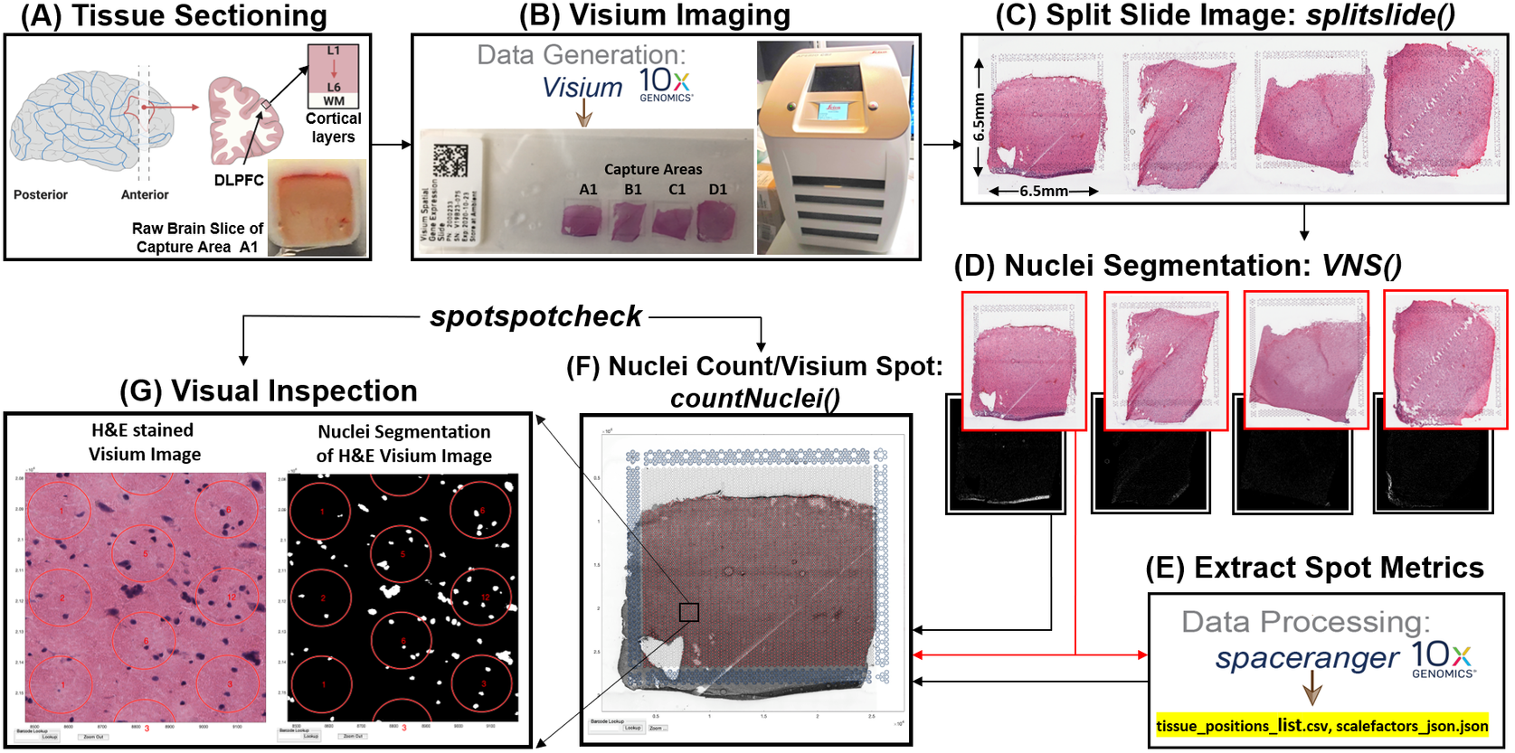
To align the sequencing files containing gene expression information with specific spatial locations (i.e., spots) on the image, users must employ the SpaceRanger software provided by 10× Genomics.(8) Using the fiducial frame on the image as reference, SpaceRanger uses the downsized TIFF files produced by the splitSlide function(24) as input to extract the barcode identifier (ID), pixel (X, Y) centroid location, and radius of each spot. SpaceRanger does not extract any information from the image beyond the presence or absence of tissue at a particular location. The output of SpaceRanger is a list of tissue positions (.csv) and the scale factors (.json) (named as tissue_positions_list.csv and scalefactors_json.json by default) to enable the quantification of gene expression in a spatial context. Further information regarding the workflow and implementation of SpaceRanger(8) is available on our accompanying website: http://research.libd.org/VistoSeg/step-3-spaceranger.html. To facilitate extraction of relevant imaging metrics at the same spatial locations (spots) queried for gene expression, VistoSeg uses the output .csv and .json files from SpaceRanger to build the spot grid on the image and enable the extraction of image-based metrics (e.g., nuclei count, percentage spot covered by nuclei) for each spot location (Figure 2e). The image-based information and the gene expression-based data are grouped together using the spot barcode identifier, which enables the quantification of gene expression and morphology metrics in a spatial context.
To segment nuclei from the H&E image (Figure 3a), we performed Gaussian smoothing and then applied contrast adjustments (Figure 3a) to enhance nuclei visibility in the image (Figure 3b). The enhanced image was then converted from RGB color space to CIELAB color space, also called L*a*b color space (Figure 3c). L*a*b color space is defined by: “L,” luminosity layer measures lightness from black to white; “a,” chromaticity layer measures color along the red–green axis; and “b,” chromaticity layer measures color along blue–yellow axis. CIELAB color space enables the quantification of the individual color gradients that are visually observable across the image. The a*b color space is extracted from the L*a*b-converted image and used as input to K-means clustering with the MATLAB function imsegkmeans (Figure 3d), along with the number of color gradients (k) that were visually identified in the image. The function output creates a binary mask for each color gradient (k) in the image. Given that nuclei in H&E images have a bright color that can be easily differentiated from the background, we used a binary mask generated from the nuclei color gradient for initial nuclei segmentation to identify nuclei as regions of interest (ROIs; Figure 3d, cluster 3, Figure 3d’). We combined these steps (Figure 3a–d’) into a function termed VNS (Visium Nuclei Segmentation).
VistoSeg workflow for Visium H&E image segmentation. (a) Raw histology image of human dorsolateral prefrontal cortex. (b) Gaussian smoothed and contrast-adjusted image of the raw histology image in (a). (c) Enhanced image from (b) converted from RGB color space to L*a*b color space. (d) Different color gradients (k = 5) identified by the MATLAB function imsegkmeans applied to the raw histology image. Cluster 3 corresponded to the nuclei, stained blue in the raw histology image. (d’) An inset of nuclei cluster 3 in (d). (e) Output of refineVNS from nuclei cluster 3 (d’). The refineVNS function allows for separation of adjacent nuclei. (f) Final binary nuclei segmentation obtained from (e).
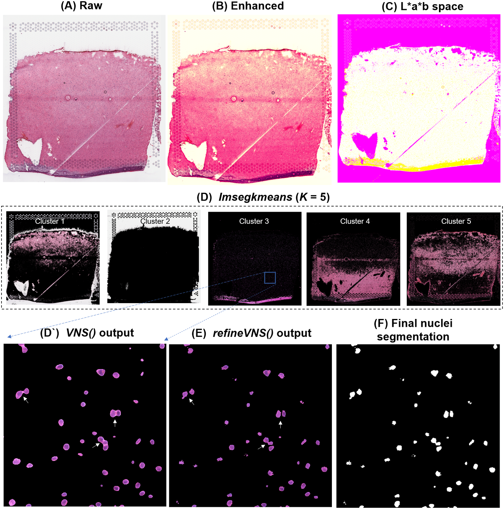
Due to the smoothing step applied, the nuclei edges are blurred, and hence nuclei in close proximity to one another are segmented as a single ROI (Figure 3d’). To further refine these segmentations to detect and quantify individual nuclei (Figure 3f), we created a second function (termed refineVNS) that extracts the intensity of the pixels from the binary mask of nuclei generated by VNS and applies intensity thresholding(Reference Raju and Neelima25) to separate the darker nuclei regions at the center from the lighter regions at the borders (Figure 3e). The final segmentation output is a binary image. The use of our VNS and refineVNS function results in segmentation of individual cell bodies in human DLPFC tissue (Figures 2g and 3d–f).
2.2. Multichannel fluorescent image processing
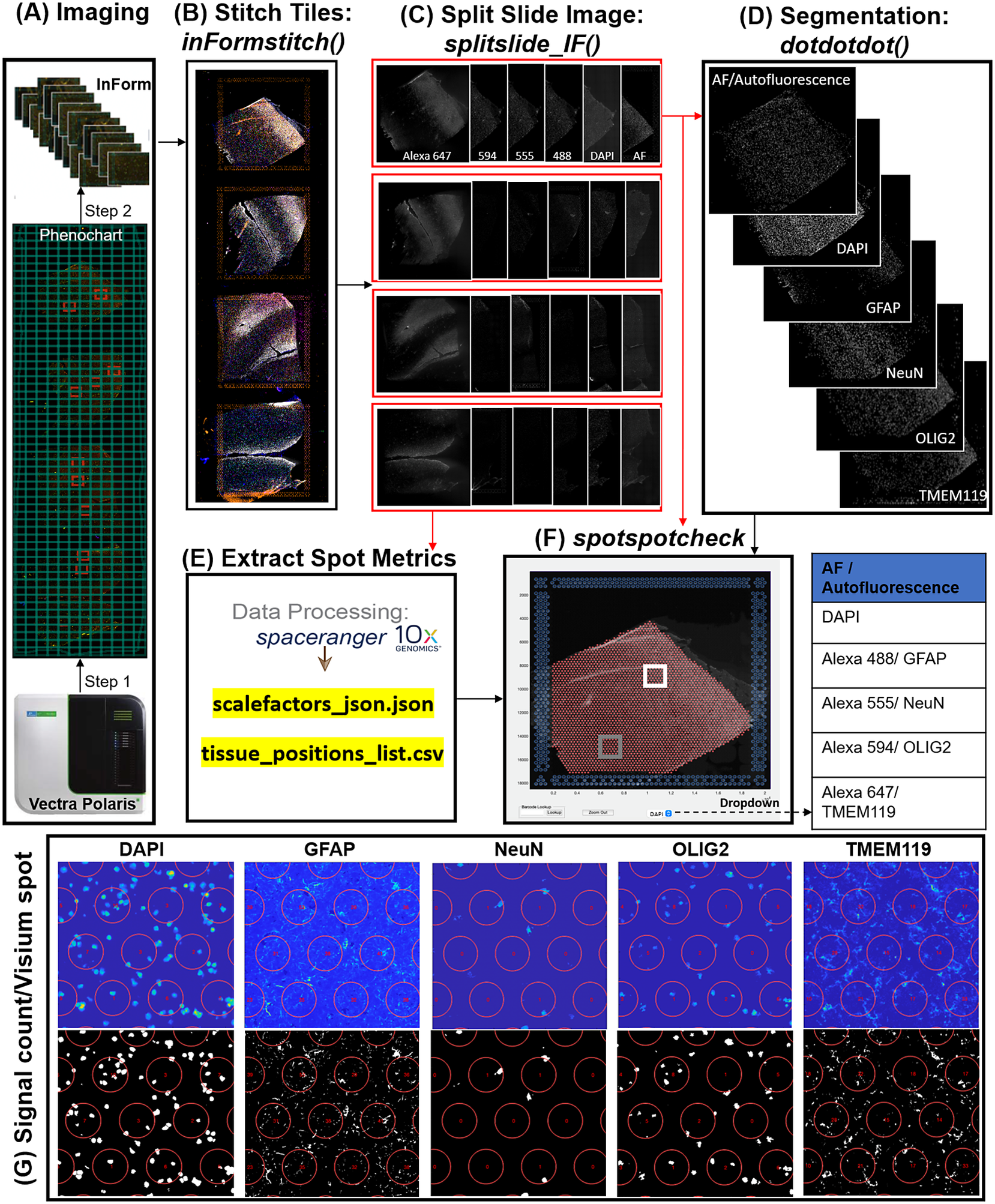
In the Visium-SPG platform, samples are subjected to immunofluorescent antibody labeling to detect specific proteins of interest, thereby generating proteomic data that can be quantified and integrated with transcriptomic data. We collected four individual tissue sections of the human dorsolateral prefrontal cortex (DLPFC) spanning the six cortical layers and white matter and performed the Visium-SPG workflow (Figure 4). To visualize cellular composition and cell type distribution across the tissue section, samples were immunostained with four established cell type markers: NeuN (Alexa 555) for neurons, TMEM119 (Alexa 647) for microglia, GFAP (Alexa 488) for astrocytes, and OLIG2 (Alexa 647) for oligodendrocytes. Immunofluorescent images were acquired using a Vectra Polaris slide scanner (Akoya Biosciences) and processed to decompose the multispectral profiles (Figure 4a).(26, 27) The final image outputs were spectrally unmixed multichannel TIFF tiles of the entire slide (~600 tiles). These individual tiles were stitched to recreate a multichannel TIFF image spanning the whole slide (Figure 4b) using the X and Y coordinates of each tile, as saved in the filename, to position tiles (inFormStitch). Next, this image was split along the Y-axis into four individual capture area images in multichannel TIFF format (splitSlide_IF; Figure 4c). We then segmented each fluorescent channel to identify ROIs (Figure 4d) as previously described.(Reference Maynard, Tippani, Takahashi, Phan, Hyde, Jaffe and Martinowich28) Finally, we used the countNuclei function to quantify the size, intensity and location of segmented signals in each channel for integration with gene expression data (Figure 4e). The output table from countNuclei has two columns per channel by default: (1) count of segmented ROIs per Visium spot and (2) proportion of the spot covered by the segmented signal. Other user-defined metrics, including mean fluorescent intensity per spot or mean intensity of segmented ROIs for each channel within a spot, can also be extracted. Quantification of immunofluorescent signals in white matter of the dorsolateral prefrontal cortex (Figure 4g) is consistent with our expectation of higher counts for glial cells stained by TMEM119 (microglia), GFAP (astrocytes) and OLIG2 (oligodendrocytes) compared to the neuron-enriched gray matter (Supplementary Figure 1).
VistoSeg workflow for Visium-SPG immunofluorescent image processing and segmentation. (a) Multispectral immunofluorescent images of the gene expression slide from the Visium-SPG workflow were acquired using a Vectra Polaris slide scanner (Akoya). All arrays on the slide were annotated as a single selection using Phenochart software (Akoya) and split into multiple tiles. Each tile was spectrally unmixed into multichannel TIFFs using inForm software (Akoya) by applying spectral fingerprints specific for each fluorophore. Autofluorescence was separated into its own channel. (b) After unmixing, the tiles from (a) were put into the VistoSeg preprocessing workflow and stitched using the inFormstitch function to recreate a multichannel TIFF of the whole slide. (c) The recreated multichannel TIFF was then split into individual arrays using splitSlide_IF. (d) Representative segmentation for capture area A1. Nuclei segmentation to identify fluorescent signal for the nucleus (DAPI) and each labeled protein (GFAP, NEUN, OLIG2, TMEM119) was performed by integrating functions from our previously published software, dotdotdot.(Reference Maynard, Tippani, Takahashi, Phan, Hyde, Jaffe and Martinowich28) (e) Using the split images from (c), Space Ranger (10× Genomics) was used to align multiplex fluorescent imaging and gene expression data and obtain extracted spot metrics (Visium spot diameter, spot spacing and spot coordinates) from each image in the “tissue_positions_list.csv” and “scalefactors_json.json” files. (f) The spotspotcheck GUI in VisotSeg provides a dropdown menu for each fluorescent channel in the multichannel TIFF (labeled by the spectral profile assigned to each protein of interest: DAPI, GFAP, NeuN, OLIG2, TMEM119 in this example). It allows for visual inspection by hovering over different regions in the image. For example, we explored the white matter (white square) and gray matter (gray square) in this representative sample. (g) The signal count per gene expression spot computed by countNuclei on the white matter (white square in f) confirms increased abundance of OLIG2, GFAP and TMEM119 staining, and relative depletion of NeuN staining, in line with expectations.
2.3. Integration of segmentation output with gene expression spot location
We generated an additional function (termed countNuclei) to calculate the number of nuclei residing within each spot. This function uses the point-in-polygon concept to calculate the number of nuclei per spot by integrating the coordinate information obtained from SpaceRanger with the segmentation mask to calculate the number of nuclei per spot. The countNuclei function accepts segmentation from alternative methods, if saved in a “.mat” format. The output of this function is a table that contains the number of nuclei and the percentage nuclei coverage per gene expression spot, which can be exported as a .csv file for each sample to be used in downstream analyses. Two types of nuclei counts are provided per spot, based on the two possible measurement criteria for calling presence/absence of nuclei: (1) inclusion of the centroid of the ROI within the spot, (2) user-defined threshold for the number of pixels necessary to count a cell as within the spot.
To enable the user to visually inspect nuclei segmentation output, we developed a GUI termed spotspotcheck. This GUI reconstructs and overlays the spot grid, generated using the output of SpaceRanger, onto the original image and the binary segmentation, generated using the output of refineVNS, to display the nuclei count in each spot. The spotspotcheck GUI supports both H&E images (Figure 2g and Supplementary Figures 2 and 3) and immunofluorescent images (Figure 4f,g, Supplementary Figure 1). Additionally, the GUI provides a dropdown menu (Figure 4f) to select different channels in the multichannel TIFF image. This allows the user to (1) toggle between the nuclei segmentation and images, (2) search for spots with specific spatial barcode IDs, and (3) zoom in and out to a specific location on the image. The user can visualize the nuclei count information by checking the “Get cell counts” option in the spotspotcheck start window. spotspotcheck enables users to perform bidirectional visual inspection, meaning that the user can evaluate morphological features in the high-resolution image and verify segmentation accuracy. Alternatively, the user can visually inspect whether gene expression patterns are related to any image features by querying specific spots through their barcode ID.
Following alignment of gene expression with image-based data, the number of nuclei present in each gene expression spot can be integrated into downstream analysis, such as creating a SpatialExperiment (spe) object,(Reference Righelli, Weber, Crowell, Pardo, Collado-Torres, Ghazanfar, Lun, Hicks and Risso29) which incorporates image-based quantifications, along with other variables, into the spot-level information. The nuclei count can then be used to perform quality control procedures and downstream analysis at the spot level. For example, during quality control, spots with an abnormally high nuclei count can be excluded.(Reference McCarthy, Campbell, Lun and Wills30) Furthermore, the nuclei count along with the spot-level gene expression matrix are required inputs for spot deconvolution methods such as Tangram.(Reference Biancalani, Scalia, Buffoni, Avasthi, Lu, Sanger, Tokcan, Vanderburg, Segerstolpe, Zhang, Avraham-Davidi, Vickovic, Nitzan, Ma, Subramanian, Lipinski, Buenrostro, Brown, Fanelli, Zhuang and Regev20)
3. Discussion
VistoSeg leverages the MATLAB Image Processing Toolbox(31) to provide user-friendly functionality for processing, analysis and interactive visualization of both H&E and fluorescent images generated in conjunction with the Visium platform. A major feature of the VistoSeg pipeline is the quantification and localization of detected ROIs in H&E images (Visium-H&E workflow) or each individual fluorescent channel (Visium-SPG workflow). VistoSeg extracts multiple user-defined metrics, including number of cells per spot, percentage of a spot occupied by cells or proteins of interest, mean fluorescent intensity in a spot, and mean fluorescent intensity of the segmented regions in the spot to aid in the interpretation and utility of SRT data.
This quantitative output from VistoSeg can be integrated with spatial gene expression data to improve spot-level resolution and add biological insights to downstream analyses. For example, using H&E images of the human dorsolateral prefrontal cortex analyzed with VistoSeg, we identified “neuropil” spots lacking cell bodies, which we hypothesized were enriched for neuronal processes. We confirmed this hypothesis by demonstrating that these “neuropil” spots are enriched for genes previously shown to be expressed in synaptic terminals.(Reference Maynard, Collado-Torres, Weber, Uytingco, Barry, Williams, Catallini, Tran, Besich, Tippani, Chew, Yin, Kleinman, Hyde, Rao, Hicks, Martinowich and Jaffe18) VistoSeg can also be used to identify spots that contain only a single cell or specific number of cells to help refine the selection of spots used for downstream gene expression analysis. Additionally, VistoSeg can identify spots with disease-associated pathology, allowing for the analysis of gene expression changes associated with pathological alterations in local microenvironments. For example, SRT has been used to identify gene expression changes associated with amyloid beta pathology in Alzheimer’s disease.(Reference Chen, Lu, Craessaerts, Pavie, Sala Frigerio, Corthout, Qian, Laláková, Kühnemund, Voytyuk, Wolfs, Mancuso, Salta, Balusu, Snellinx, Munck, Jurek, Fernandez, Saido, Huitinga and De Strooper32) VistoSeg opens opportunities to directly incorporate different pathology-associated metrics with transcriptomic changes in diseased tissues.
Importantly, VistoSeg output can be further integrated with other software(Reference Phillip, Han, Chen, Wirtz and Wu33, Reference Logan, Shan, Bhatia and Carpenter34) to identify and classify specific cell types based on nuclear or cellular morphology. For example, spatial domains corresponding to specific tumor pathology can vary in cell size, shape and density across tissue sections. Identification of these pathological lesions can provide important insights into the role of spatially restricted gene expression in disease progression.(Reference Chang, He, Wang, Chen, Li, Liu, Yu, Su, Ma, Allen, Lin, Sun, Liu, Javier Otero, Chung, Fu, Li, Xu and Ma35, Reference Palla, Spitzer, Klein, Fischer, Schaar, Kuemmerle, Rybakov, Ibarra, Holmberg, Virshup, Lotfollahi, Richter and Theis36) We further anticipate that outputs of VistoSeg can be used to calculate other tissue parameters, such as cell density, for incorporation into unsupervised clustering approaches to identify data-driven spatial domains more directly related to cytoarchitecture. Given that a single Visium spot contains multiple cells with several cell types, spot deconvolution algorithms are rapidly being developed to predict the proportion of different cell types in each spot.(Reference Sang-aram, Browaeys, Seurinck and Saeys37, Reference Li, Zhou, Li, Chen, Liao, Zhang, Zhang, Wang, Sun and Gao38) Spot deconvolution algorithms generally require Visium gene expression data (with or without cell counts) and single cell/nucleus RNA-seq gene expression data from the same tissue type (Supplementary Figure 4). Some spot deconvolution software, including Tangram(Reference Biancalani, Scalia, Buffoni, Avasthi, Lu, Sanger, Tokcan, Vanderburg, Segerstolpe, Zhang, Avraham-Davidi, Vickovic, Nitzan, Ma, Subramanian, Lipinski, Buenrostro, Brown, Fanelli, Zhuang and Regev20) and Cell2Location,(Reference Kleshchevnikov, Shmatko, Dann, Aivazidis, King, Li, Elmentaite, Lomakin, Kedlian, Gayoso, Jain, Park, Ramona, Tuck, Arutyunyan, Vento-Tormo, Gerstung, James, Stegle and Bayraktar19) require the user to input the number of cells per spot, while others do not require this information. However, spot deconvolution results were improved for methods that include cell counts per spot compared to methods that do not use any image-level spot metrics.(Reference Huuki-Myers, Spangler, Eagles, Montgomery, Kwon, Guo, Grant-Peters, Divecha, Tippani, Sriworarat, Nguyen, Ravichandran, Tran, Seyedian, PsychENCODE, Hyde, Kleinman, Battle, Page, Ryten and Maynard39) Spot deconvolution algorithms have already begun to leverage cell counts from imaging data,(Reference Hu, Li, Coleman, Schroeder, Ma, Irwin, Lee, Shinohara and Li15) and we anticipate that more quantitative outputs from software such as VistoSeg can improve the identification of biologically relevant spatial domains and associated cell type proportions.
In summary, VistoSeg was designed to address an image analysis gap in the most widely used, commercially available SRT-processing pipeline, the Visium Spatial Gene Expression platforms. However, we note some limitations with Vistoseg, such as large memory requirements (~75 GB) for loading and saving images. Furthermore, the VNS function requires manual user inputs and cannot currently be fully automated. However, we note that similar existing image analysis software, such as HALO,(40) QuPath(Reference Bankhead, Loughrey, Fernández, Dombrowski, McArt, Dunne, McQuaid, Gray, Murray, Coleman, James, Salto-Tellez and Hamilton9) and Squidpy,(Reference Palla, Spitzer, Klein, Fischer, Schaar, Kuemmerle, Rybakov, Ibarra, Holmberg, Virshup, Lotfollahi, Richter and Theis36) also have limitations on processing times and parametrization, and there are currently no available modules to support integration of gene expression data with segmented images. While Vistoseg was primarily designed for the available Visium platforms, we anticipate its functions will be relevant to other NGS-based SRT platforms should future assays become available from other vendors. We note that among all current SRT technologies, Visium is by far the leading platform in the field(Reference Moses and Pachter6) with over 60 institutions utilizing the technology at the time of publication, further supporting the need for improved imaging-processing tools.
While we recognize that MATLAB is closed source, it is compatible with open science(41) and readily available to academic users. MATLAB supports the ability to read images from various proprietary file formats from multiple instrument manufacturers. All code for VistoSeg is freely available (see Data Availability), and the main output of VistoSeg is in .csv format, which can be easily incorporated into commonly used pipelines for analysis of SRT data such as R objects for SpatialExperiment(Reference Righelli, Weber, Crowell, Pardo, Collado-Torres, Ghazanfar, Lun, Hicks and Risso29) and Seurat,(Reference Hao, Hao, Andersen-Nissen, Mauck, Zheng, Butler, Lee, Wilk, Darby, Zager, Hoffman, Stoeckius, Papalexi, Mimitou, Jain, Srivastava, Stuart, Fleming, Yeung, Rogers and Satija42) or Python objects for AnnData.(Reference Virshup, Rybakov, Theis, Angerer and Wolf43) In addition, conversion utilities like zellkonverter(Reference Zappia44) facilitate intercommunication among these programing languages. As other packages are made available that expand on the key infrastructure provided by SpatialExperiment, VistoSeg will continue to be compatible with them.
4. Conclusion
We developed VistoSeg as a user-friendly image-processing toolkit, which is optimized for NGS-based SRT technologies, including the commercially available Visium platforms, to facilitate integration of the rich anatomical and/or proteomic data in the H&E and fluorescent images accompanying spatial gene expression data. VistoSeg performs automatic splitting of whole-slide images for downstream data processing and allows for segmenting, visualizing, and quantifying individual high-resolution raw histology and immunofluorescent images. The pipeline is easily adaptable for images obtained from Visium H&E and Visium-SPG workflows from different tissues, organs and species. The pipeline is available at http://research.libd.org/VistoSeg and includes a detailed tutorial with example data for implementing VistoSeg.
5. Materials and methods
5.1. Post-mortem human brain tissue
Post-mortem human brain tissue was obtained at the time of autopsy with informed consent from the legal next of kin, through the Maryland Department of Health IRB protocol #12–24, and from the Department of Pathology of Western Michigan University Homer Stryker MD School of Medicine, the Department of Pathology of University of North Dakota School of Medicine and Health Sciences, and the County of Santa Clara Medical Examiner-Coroner Office in San Jose, CA, all under the WCG protocol #20111080. Details of tissue acquisition, handling, processing, dissection, clinical characterization, diagnoses, neuropathological examinations and quality control measures have been described previously.(Reference Lipska, Deep-Soboslay, Weickert, Hyde, Martin, Herman and Kleinman45)
5.2. Tissue preparation and image acquisition for Visium H&E
Tissue was cryosectioned on a Leica 3050 cryostat at 10-micron thickness and collected onto a Visium Spatial Gene Expression slide (catalog no. 2000233; 10× Genomics). H&E staining was performed on fresh-frozen tissue according to manufacturer’s instructions to identify nuclei (dark blue/purple) and cytoplasm (pink) in the tissue section. The two stains combine to label features of the tissue in various shades of pink and blue. Thus, the range of colors present in the staining depends on the cellular composition of the tissue. Following H&E staining, the Visium slide was imaged on a Leica Aperio CS2 slide scanner (Figure 1b) equipped with a color camera and a 20×/0.75 NA objective with a 2× optical magnification changer, which meets the recommended microscopy specification outlined by Visium Spatial Gene Expression Imaging Guidelines from 10× Genomics.(46) This protocol produced high-resolution (0.253 μm per pixel) images for downstream analysis.
5.3. Immunofluorescent staining and image acquisition for Visium-SPG
Immunofluorescent staining was performed according to the manufacturer’s instructions (catalog no.CG000312 Rev C; 10× Genomics). Briefly, post-mortem human dorsolateral prefrontal cortex (n = 4 tissue sections from four individual donors) was microdissected and cryosectioned at 10-micron thickness. Sections were mounted on a Visium Spatial Gene Expression Slide (catalog no. 2000233; 10× Genomics), fixed in prechilled methanol, blocked in BSA-containing buffer, and incubated for 30 min at room temperature with primary antibodies against NeuN, TMEM119, GFAP, and OLIG2 (mouse anti-NeuN antibody conjugated to Alexa 488 [Sigma Aldrich; Cat# MAB377X, 1:100], rabbit anti-TMEM119 antibody [Sigma Aldrich; Cat# HPA051870, 1:20], rat anti-GFAP antibody [Thermofisher; Cat# 13-0300, 1:100], and goat anti-OLIG2 antibody [R&D systems; Cat# AF2418, 1:20]). Following washes, appropriate secondary antibodies were applied for 30 min at room temperature (donkey anti-rabbit IgG conjugated to Alexa 555 [Thermofisher; Cat# A-31572, 1:300], donkey anti-rat IgG conjugated to Alexa 594 [Thermofisher; Cat# A-21209, 1: 600], and donkey anti-goat IgG conjugated to Alexa 647 [Thermofisher, Cat# A-21447, 1:400]). DAPI (Thermofisher; Cat# D1306, 1:3000, 1.67 μg/ml) was applied for nuclear counterstaining. The slide was coverslipped with 85% glycerol and imaged on a Vectra Polaris slide scanner (Akoya Biosciences) at 20× magnification with the following exposure time per given channel: 2.1 ms for DAPI, 143 ms for Opal 520, 330 ms for Opal 570, 200 ms for Opal 620, 1070 ms for Opal 690, 100 ms for Autofluorescence prior to downstream transcriptomics. Slide scanning generated a qptiff image file, which was then selected for a region of interest (ROI) in Phenochart software (Akoya Biosciences) with an annotation tool outlining the entire slide. The resulting boundaries created a grid line of multiple tiles that made up the entire demarcated ROI. The annotated qptiff image was then processed in InForm software (Akoya Biosciences) and subjected to linear unmixing with the reference spectral profiles of corresponding fluorophores. InForm performs linear unmixing tile by tile while producing linearly unmixed tile images in tiff. The subsequent individual tile images were processed through the VistoSeg pipeline to extract final quantitative output.
5.4. cDNA synthesis and library preparation
Following imaging, gene expression libraries were generated on the slide, followed by denaturing and amplification. Standard Illumina sequencing was performed according to manufacturer’s specifications.
5.5. System requirements and availability for VistoSeg
Project name: VistoSeg
Project home page: https://github.com/LieberInstitute/VistoSeg, http://research.libd.org/VistoSeg/
Operating system(s): MAC, Windows, LINUX
Programming language: MATLAB
Other requirements:
(1) MATLAB Image Processing Toolbox
(2) MATLAB v2019a or later
(3) Minimum ~ (3*raw image) 80 GB RAM for the initial (splitSlide) step and <16GB for all the remaining steps
(4) SpaceRanger (10× Genomics) v1.0 or higher
(5) Loupe browser (10× Genomics) v5 or higher
License: GNU GENERAL PUBLIC LICENSE, Version 3, June 29, 2007.
Any restrictions to use by nonacademics: license required.
Glossary of terms
- 10× Genomics:
-
commercial vendor producing Visium technology
- barcode identifier (ID):
-
unique genomic sequence for each spatially restricted position on a Visium slide
- CIELAB or L*a*b:
-
color model incorporating perceptual lightness (L) with colors unique to human vision (red, green, blue and yellow), to enable the detection and calculation of visibly evident changes in color patterns
- countNuclei:
-
a function used to generate the nuclei count file that stores the information about the number of segmented nuclei in each spot
- GUI:
-
graphical user interface
- imsegkmeans:
-
a MATLAB function that uses K-means clustering-based image segmentation
- inFormstitch:
-
a MATLAB function used to stitch all spectrally unmixed individual tiles of a Visium-SPG immunofluorescent slide image to recreate a multispectral TIFF image
- Loupe browser:
-
Primary Visualization software provided by 10× Genomics
- MATLAB:
-
MATrix LABoratory
- NGS:
-
next-generation sequencing
- refine(VNS):
-
a function that refines the segmentation done using VNS function
- RGB:
-
red, green, blue color model
- ROI:
-
region of interest
- SpaceRanger:
-
analysis software provided by 10× Genomics to align transcript reads to the genome and assign them to a Visium spot
- splitslide:
-
a MATLAB function used to split the whole-slide Visium-H&E image into individual capture arrays
- splitSlide_IF:
-
a MATLAB function that splits the multispectral TIFF image obtained using inFormStitch function into individual capture arrays
- spotspotcheck:
-
a GUI that allows the user to visualize and quantify nuclei segmentation results performed using VNS and refineVNS
- SRT:
-
spatially resolved transcriptomics
- Visium H&E:
-
Visium assay using H&E staining.
- Visium-SPG:
-
Visium Spatial Proteogenomics assay using immunofluorescent staining
- VNS:
-
a MATLAB function that segments nuclei for Visium H&E images
Supplementary material
The supplementary material for this article can be found at https://doi.org/10.1017/S2633903X23000235.
Data availability statement
Examples of code, data, output and results are available at http://research.libd.org/VistoSeg/index.html#data-availability and https://github.com/LieberInstitute/VistoSeg.(47) All inputs and outputs are available through Figshare.(Reference Tippani, Divecha, Weber, Kwon, Spangler, Jaffe, Hicks, Martinowich, Collado-Torres, Page and Maynard48) Public datasets provided by 10× Genomics.(49)
Acknowledgments
We thank Anthony Ramnauth (LIBD) and Uma Kaipa (LIBD) for testing code functionality. We thank the “spatialLIBD” team (LIBD and JHU) for their feedback on VistoSeg and testing the software across multiple datasets. We thank Amy Deep-Soboslay and her diagnostic team for curation of brain samples. We thank the neuropathology team for their assistance with tissue dissection. We thank the physicians and staff at the brain donation sites and the generosity of donor families for supporting our research efforts. Finally, we thank the families of Connie and Stephen Lieber and Milton and Tamar Maltz for their generous support to this work. A preprint of this work is available on bioRxiv: https://doi.org/10.1101/2021.08.04.452489.
Funding statement
This work was supported by the Lieber Institute for Brain Development and the National Institute of Health grants U01MH122849 and R01MH126393.
Competing interest
A.E.J. is now a full-time employee at Neumora Therapeutics, a for-profit biotechnology company, which is unrelated to the contents of this manuscript. J.L.C. is now a full-time employee at Delfi Diagnostics, a for-profit biotechnology company, which is unrelated to the contents of this manuscript. Their contributions to the manuscript were made while previously employed by the Lieber Institute for Brain Development. All other authors declare no competing interests.


 Open access