


Introduction
Habitat selection is influenced by a number of proximate and ultimate factors (Block and Brennan Reference Block and Brennan1993), including habitat structures, floristics, competition, food availability and predation risk (MacArthur and MacArthur Reference MacArthur and MacArthur1961, Southwood Reference Southwood1977, Noon Reference Noon1981, Muller et al. Reference Muller, Stamps, Krishnan and Willits1997). The prevalent definition of habitat selection is the disproportionate use of environmental conditions to influence survival and ultimate fitness (Block and Brennan Reference Block and Brennan1993), which takes place at multiple spatial and temporal scales (Johnson Reference Johnson1980, Kotliar and Wiens Reference Kotliar and Wiens1990). Landscape-scale features (macrohabitat) are correlated with the distribution and abundance of populations and often describe discrete arrays of, e.g., specific vegetation types. Particular features of an environment that act as proximal cues to stimulate settling of an individual animal constitute its microhabitat which can represent specific habitat patches or individual home ranges (Block and Brennan Reference Block and Brennan1993). When investigating habitat selection, it is widely recommended to include more than one spatial scale, preferably within a nested hierarchy (Wiens et al. Reference Wiens, Rotenberry and Van Horne1987, Kotliar and Wiens Reference Kotliar and Wiens1990) as it can be difficult or impossible to determine in advance the most ecologically relevant scale for different environmental variables.
The current knowledge of Baillon’s Crake Zapornia pusilla ecology is very limited, comprising only general information about the species’ ecological requirements and habitat selection. Few specific studies exist, which are all descriptive in nature (Noll Reference Noll1924, Szabó Reference Szabó1970) and compendia mostly report anecdotal observations or refer to other Palaearctic Porzana and Zapornia species (e.g. Glutz von Blotzheim et al. Reference Glutz von Blotzheim, Bauer and Bezzel1994). Typical habitats include palustrine wetlands, freshwater to saline, with dense vegetation such as marshes, floodplains, inundated grasslands and irrigated crops (Taylor and Van Perlo Reference Taylor and Van Perlo1998). Suitable wetlands are often seasonally and only shallowly flooded with water levels ranging from a few to 30 cm (Glutz von Blutzheim et al. Reference Glutz von Blotzheim, Bauer and Bezzel1994, Taylor and Van Perlo Reference Taylor and Van Perlo1998). However, outside the breeding season the species is reported to occur in a wider variety of habitats with water levels up to 2 m (Marchant and Higgins Reference Marchant and Higgins1993). Vegetation cover is typically dominated by relatively fine-stemmed sedge and grass species, including the genera Carex, Cyperus, Eleocharis, Juncus, Scirpus and Phalaris (Szabó Reference Szabó1970, Glutz von Blotzheim et al. Reference Glutz von Blotzheim, Bauer and Bezzel1994, Taylor and Van Perlo Reference Taylor and Van Perlo1998) which form a dense and usually uniform vegetation cover. Nesting locations are often associated with tussocks of e.g. Eleocharis spp. or tall forbs such as Althaea officinalis (Szabo Reference Szabó1970) and nests consist predominantly of fresh and soft plant material (Glutz et al. Reference Glutz von Blotzheim, Bauer and Bezzel1994). Glutz et al. (Reference Glutz von Blotzheim, Bauer and Bezzel1994) described the habitats occasionally comprising ditches and sparsely vegetated shallows and Taylor and Van Perlo (Reference Taylor and Van Perlo1998) reported that the species normally forages in unvegetated spots. But the significance of edge structures, open water bodies and other small-scale features for Baillon’s Crake habitat has not been investigated yet. Likewise, virtually nothing is known about the extent and dynamics of the species’ home ranges or population densities. Taylor (Reference Taylor, Harrison, Allan, Underhill, Herremans, Tree, Parker and J. Brown1997) provided the only estimate for breeding Baillon’s Crakes for a wetland in KwaZulu-Natal, South Africa, while densities in European breeding grounds are assumed to be generally marginal (e.g. Dies and Dies Reference Dies, Dies, Marti and Moral2003) owing to the small European population which comprises only 740–3,200 breeding pairs (BirdLife International 2004).
Across both its European and African ranges, the species is considered to be declining as a consequence of severe habitat degradation, e.g. the cultivation and drainage of ephemeral wetlands (Koshelev Reference Koshelev and Tucker1994, Taylor and Van Perlo Reference Taylor and Van Perlo1998). Accordingly, only a handful of observations are reported annually both for its Palaearctic and Afrotropical breeding grounds (e.g. DAK 2010). All the more remarkable was the discovery of a potentially large breeding population of Baillon’s Crake in the Senegal River Delta, north-west Senegal (Seifert et al. Reference Seifert, Becker and Flade2012), where the species was only assumed to spend the non-breeding season (Roux and Morel Reference Roux and Morel1966). Based on capture data from 2007, Flade (Reference Flade2008) presumed the floodplains of the Parc National des Oiseaux du Djoudj (PNOD) to accommodate the majority if not the entire European population during the Northern hemisphere winter months. By now, the area’s significance exclusively as a non-breeding site for European migrants is questionable after the observation of many individuals reproducing both in the PNOD and Diawling National Park (Mauritania) at that time (Seifert et al. Reference Seifert, Becker and Flade2012, Reference Seifert, Haase, Van Wilgenburg, Voigt and Schmitz Ornés2016, Seifert & Sidaty Reference Seifert and Sidaty2013). However, local Baillon’s Crake abundance may surpass by far any other number estimated for known populations, which would underline the relevance of the PNOD and adjacent floodplains throughout the Senegal River Delta as important refuge.
Knowledge of a species’ ecological requirements is a prerequisite for effective conservation (e.g. Luck Reference Luck2002), particularly if the species is assumed to be declining due to modification and degradation of its habitats. Information about habitat suitability allows both the inference of specific habitat management measures as well as models to estimate potential distribution or population sizes (Guisan and Zimmermann Reference Guisan and Zimmermann2000) which can facilitate the set-up of conservation priorities. Accordingly, the aim of this study was to (1) determine factors that influence occurrence of Baillon’s Crakes both on a macro- as well as microhabitat scale. Thereby we address the question whether structural characteristics of vegetation or plant species composition are more relevant for the species’ habitat selection. Furthermore, we intend to (2) predict the extent of suitable habitat and (3) estimate the potential maximum population size of Baillon’s Crakes within and in the vicinity of the PNOD in order to assess the significance of the Senegal River Delta for the species.
Material and methods
Study area
Our fieldwork was performed within and north of the PNOD (16°20’N, 16°12’W), the so-called Djoudj area (Figure 1). The study area (in total 41,184 ha) comprises a network of former tributaries of the Senegal River, seasonal lakes and shallowly inundated floodplains which are nowadays artificially flooded during the rainy season between July and October (Fall et al. Reference Fall, Hori, Kann and Diop2003). In the course of the subsequent dry season, the majority of the area, vast grass and sedge marshes, falls dry successively. The typical vegetation consists of ephemeral salt-resistant plant species such as Eleocharis mutata, Oryza longistaminata, Scirpus maritimus, S. littoralis and Sporobolus robustus. Cattail stands Typha australis prevail at locations with stronger influence of freshwater and along the banks of the Senegal River.
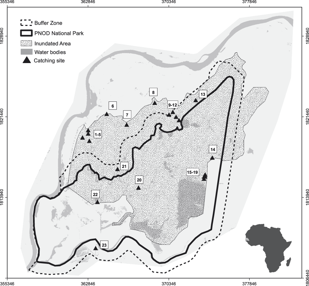
Figure 1. Study area (Djoudj) and location of 23 study sites (1 -5 = Tiguet I – V, 6 = Tiguet East, 7 = Debi West, 8 = Debi East, 9-12 = Crocodil I – IV, 13 = Diadiam, 14 = Grand Lac North, 15-19 = Grand Lac I – V, 20 = Gainthe, 21 = Tiguel, 22 = Lac Tantale, 23 = Typha).
Study sites and capture of Baillon’s Crakes
Baillon’s Crakes were caught in 23 geographically separated study sites between December and March during our field work periods in the dry seasons 2009 (n = 10), 2009/2010 (n = 9) and 2013 (n = 4) (Figure 1). The capture sites were selected by sampling different vegetation types all over the study area which a) provided enough vegetation cover and b) were sufficiently inundated with water levels varying from five to 40 cm. Based on literature on habitat requirements (e.g. Szabó Reference Szabó1970, Taylor and Van Perlo Reference Taylor and Van Perlo1998) these settings were regarded as minimum preconditions for the potential presence of Baillon‘s Crakes. Birds were caught with a set of 30 – 40 cage traps (Bub Reference Bub1995) which were installed at regular intervals of approximately 10 m along transect lines within the study sites. Captured birds were aged into adult, juvenile and chick, and body measurements as well as respective trap coordinates were recorded.
Telemetry
In total, 23 adult birds with body mass >40 g were equipped with 1.3 g lightweight radio-transmitters (PIP3 single celled tags, Biotrack Ltd.) in the field seasons 2009 (n = 7) and 2009/2010 (n = 15) at the three study sites Grand Lac (GL), Tiguet (TG) and Debi (DB, only one individual in 2009). Transmitters were attached using a leg-loop harness following Haramis and Kearns (Reference Haramis and Kearns2000). Radio-tracking was conducted with a hand-held three-element Yagi-antenna connected to a Sika receiver (Biotrack Ltd.). Tagged individuals were recorded starting 48 h after capture. Locations of individuals were collected every second (2010) or third day (2009) from 07h00 to 14h00 and occasionally in the afternoons from 16h00 to 19h00. Thereby we tried to obtain relocations for each individual at least three times in the course of the day with approx. 1.5 h between the fixes. Relocations were assessed by triangulation (White and Garrot Reference White and Garrott1990) using three to five bearings, and LOCATE (Nams Reference Nams2006) was used to determine Baillon’s Crake locations. All directions were recorded within five minutes to minimise errors due to the birds’ movements. Radio-tracking was performed only by N. Seifert in both field seasons.
Estimation of home ranges
Only individuals with >10 relocations and a tracking period of > five days were included in the home range estimation. As we detected large movements after capturing the birds, we did not consider the location of the respective cage traps in the analyses. Home range boundaries were calculated with a fixed kernel estimator (Hooge and Eichenlaub Reference Hooge and Eichenlaub1997) reporting the 95% kernel density home range for each Baillon’s Crake using the R-package “adehabitatHR” (Calenge Reference Calenge2006). The smoothing parameter h was estimated via the reference bandwith “href” as the number of relocations was too small for some individuals (<20) to apply a least squares cross-validation procedure (e.g. Seaman and Powell Reference Seaman and Powell1996). In order to detect directional shifts in the position of the home ranges, we calculated the centroid for each daily set of relocations per bird and measured the distances and directions between the first and last centroid.
Environmental variables
Land cover classes in GL and TG
As nearly all radio-tracked Baillon’s Crakes were followed in the two study sites Grand Lac (GL) and Tiguet (TG), we aimed at generating high resolution vegetation maps for each site to capture small-scale features which might be ecologically relevant for Baillon’s Crake habitat selection. For this purpose, we took aerial photographs during the field season 2009/2010 using a Sutton Flow kite (Kite Aerial Photography) which was flown over the sites following transects in N-S (TG) or E-W (GL) direction. A 7-megapixel point & shoot camera (Canon Powershot G6) combined with a 2 GB storage medium was mounted on a Picavet-suspension approx. 50 m underneath the kite. Imagery was obtained in 3072 x 2304 pixel images taken at a shooting frequency of one image per minute. The ground resolution of these images depends on the flying height of the kite (e.g. 5 cm at a flying height of 130 m above the ground, Becker et al. Reference Becker, Kutzbach, Forbrich, Schneider, Jager, Thees and Wilking2008). For ground verification, we installed a 30 x 30 m grid of white paper plates with known GPS position (4 m accuracy) as ground control points within the sites. These points were later used to georectify and merge the pictures into one image per site using ArcGIS 10.1 (ESRI 2015). Each site was photographed twice to ensure sufficient overlap of images.
The georectified imagery was polygonised and classified by hand, using ArcGIS, defining six classes of herbaceous vegetation types dominated by one plant species, nine classes of mixed stands, three classes of tree/shrub species as well as other land cover classes such as zones with scarce vegetation cover (<50%), unvegetated soil, open water and trampling path (Table 1, Appendix S2, S3 in the online supplentary material). Two raster maps were obtained with a resolution of 0.25 m2 per pixel cell by rasterizing the resulting land cover maps.
Table 1. Land cover classes of vegetation maps and additional structural habitat parameters for the entire Djoudj area (DJOUDJ) and study sites Grand Lac (GL) and Tiguet (TG). Fraction of land cover classes given in % of total area.
* % of 130 x 130 m pixel cells containing edge structures of respective vegetation class.

Land cover classes Djoudj area
Land cover data for the entire study area was obtained from the classification of high resolution satellite images taken in January 2011 with a resolution of 0.5 m2 (Tegetmeyer et al. Reference Tegetmeyer, Fricke and Seifert2014). The derived order synonym vegetation and land cover map with a resolution of 1 m2 per pixel cell contained six classes of dominant vegetation (Table 1) and five general land-cover classes: woody vegetation (e.g. Acacia sp., Tamarix senegalensis, Salvadora persica), sandy soil, open water, bare soil and cultivated rice paddies.
Habitat selection analyses
Habitat selection was analysed considering multiple scales, both on a population as well as an individual level following Thomas and Taylor (Reference Thomas and Taylor1993) who differentiated between three designs which correspond to different levels of selection identified by Wiens (Reference Wiens1973). While first order selection applies to the level of population and e.g. its geographic range, second and third order selection occur at the individual level, either at the scale of local sites or plot patterns in territories (second order) or patterns of utilisation (third order).
Individual level (Design II, III)
For second and third order habitat selection, we compared the use and availability of each habitat class by calculating the Manly selection ratio wj
 $${w_j}\, = \,{{{u_j}} \over {{a_j}}}$$
where uj is the proportion of use of the habitat class j and aj is the proportion of availability of this habitat class (Manly et al. Reference Manly, McDonald, Thomas, McDonald and Erickson2002). Habitat selection ratios were significant if their 95% confidence intervals did not include 1; values >1 indicated selection while values <1 indicated avoidance (Manly et al. Reference Manly, McDonald, Thomas, McDonald and Erickson2002).
Firstly, habitat use was measured for each radio-tracked individual (= 95% kernel density home range), but availability was assumed to be the same for all individuals, considering the entire extent of the respective study site (= Design II). Secondly, both use and availability of the habitat classes was measured for each individual, implying that availability varies from one animal to the other (= Design III). Accordingly, for each radio-tracked Baillon’s Crake, available habitat units correspond to the pixel cells of the 0.25 m2 vegetation maps (GL and TG) falling inside the limits of the 95% kernels. Used habitat units correspond to the pixel cells containing the relocations. To account for the GPS accuracy of ± 4 m, we extracted all pixel cells in a radius of 4 m around each relocation. In total 16 (GL) and 18 (TG) different habitat classes as well as edge length of open water bodies and trampling paths were considered (Table 1).
Population level
For modelling habitat selection on a landscape level in order to assess the extent of suitable habitat and infer a potential population size for the Baillon’s Crake in the study area, we used both logistic regression models as well as Poisson models based on capture data of the 23 study sites (Figure 1).
We subdivided the trap transects in each study site into 130 x 130 m blocs corresponding to the mean home range size of 1.77 ha (see Results) and summed up the number of Baillon’s Crakes captured within the first three days after the installation of the transect. By this, we derived two response variables comprising count and presence/absence data for a total of 108 trap transect blocs, respectively.
The values of explanatory variables were obtained from a 1.77 ha circle (r = 75.06 m) drawn around each midpoint of the transect blocs, extracting the sum of pixel cells for each of the 11 land cover classes of the study area’s vegetation map. In addition, we calculated the edge length of patches of different vegetation classes to consider effects of edge structures in our models.
The vegetation map was used to generate a 130 x 130 m raster layer for each of the vegetation and land cover classes, every pixel cell containing the sum of the underlying 1 m2 pixel cells per class. The resolution of this set of raster layers corresponded to the area sampled in each trap transect bloc.
To derive the presence probability of Baillon’s Crake in a given 130 x 130 raster cell, we used logistic regression models with a logit link function, assuming a Bernoulli distribution (McCullagh and Nelder Reference McCullagh and Nelder1989) for the response variable. A Poisson model was chosen to estimate population density for a given raster cell. As the 108 trap transect blocs were grouped into 23 geographically separated sites (Figure 1), we had to consider that transect blocs within one study site are more similar to each other than to blocs of other sites. Accordingly, we included “site” as a random factor, using generalised linear models (Bolker et al. Reference Bolker, Brooks, Clark, Geange, Poulsen, Stevens and White2009).
After controlling for collinearity, we included the following explanatory variables as main effects into our global models: ELE, ORZYA, SCL, SCM, SPORO, TYPHA, Water and WOOD as well as Edge_ELE, Edge_ORY, Edge_SCL and Edge_TYPH (Table 1). All numerical variables were centred and standardised. Model assumptions were tested by graphical analysis of residuals. We used a stepwise backward selection to choose the best model using Akaike’s information criterion corrected for small sample size (AICc, Burnham and Anderson Reference Burnham and Anderson2002; Appendix S1). To assess the predictive performance of the best models, we performed cross-validation, allocating the data into cross-validation groups corresponding to the 23 separate study sites. The models were fitted using 22 of our 23 sites and the predictive power was tested using the remaining site. The cross-validation score was calculated as the sum of the squared differences between cross-validated predictions and our observation data. The model predictions were graphically compared with the probability of presence (logistic model) and the number of the individuals of the count data (Poisson model), respectively.
Predicting the extent of suitable habitat and population size
The best (final) models were used to predict the presence probability (logistic model) and density of Baillon’s Crake (Poisson model) for each 100 x 100 raster cell. We calculated the potential population size as well as the lower and upper limit of the 95% credible interval (CI) by summing up all predicted density values. The area of potentially suitable habitat was determined by calculating the sum of all raster cells with a presence probability of >0.5. All spatial data were handled in ArcGIS 10.1 and 10.2 and the R-package “raster” (Hijmans et al. Reference Hijmans and Etten2014) and “maptools” (Bivand and Lewin-Koh Reference Bivand and Lewin-Koh2014). GLMMs were fitted using the glmer function from the “lme4” package (Bates et al. Reference Bates, Maechler, Bolker and Walker2014).
Results
Home ranges
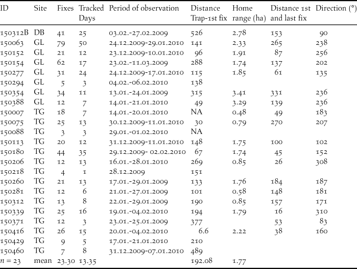
Mean home range size was 1.77 ± 0.86 ha (minimum HR: 0.48 ha, maximum HR: 3.41 ha; Table 2, Appendix S2, S3). We found no significant effect of number of fixes or tracking days on home range size (n fixes: F1,16 = 2.71, p = 0.11, n days: F1,16 = 2.39, p = 0.14). Home ranges were significantly larger in GL (Wilcoxon-test, W = 59.5, P = 0.008) with a mean of 2.42 ha compared to 1.28 ha in TG. It should be noted that, generally, some individuals in GL could be tracked over long periods (Table 2) though we did not find the number of fixes or tracking days significantly different at the two study sites (Wilcoxon-test, n fixes: W = 44.5, P = 0.12; n days: W = 39, P = 0.35).
Table 2. Key data of Baillon’s Crakes radio-tracked during the field seasons 2009 and 2009–2010 in three sites (DB = Debi, GL = Grand Lac, TG = Tiguet) within and in the vicinity of the PNOD, Senegal. Home range size is estimated by 95% fixed kernels.
Individuals moved between initial capture and first relocation on average 192.08 ± 121.45 m (e.g. Figure 2), while later movements between consecutive daily centroids during the tracking period were shorter with a mean of 35.68 ± 12.49 m. Only for three birds detected distances between capture and first relocation corresponded to the mean daily movement (Table 2). Both in GL as well as in TG a tendency was observable that centroids of daily relocations shifted towards south (Fig. 3). Eighty percent of birds radio-tracked at GL showed a south-westerly movement, while directions in TG were less distinct with 63% southerly, but also easterly and north-westerly directions (18% each). Considering only birds for which movements were >130 m (corresponding to edge length of mean home range size), movements were consistently oriented towards south and south-west (Figures 2, 3).
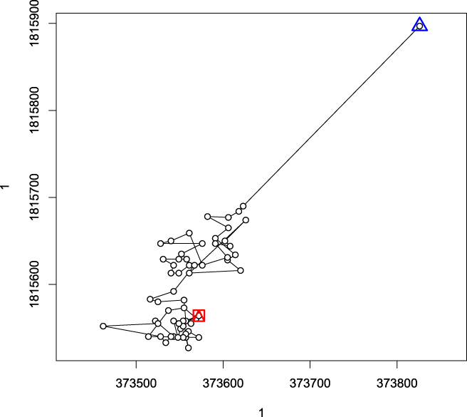
Figure 2. Individual trajectory for radio-tracked bird ID 150154. Triangle: position of the trap. Square and triangle: last relocation. Lines connect consecutive relocations.

Figure 3. Directional shifts in home ranges (first and last centroid of daily relocations). Dark grey = GL, light grey = TG. Solid lines = movements >130 m, dashed lines = movements <130 m.
Habitat selection
Individual level
Comparing the composition of land cover classes within the 17 home ranges with the study sites’ overall composition (Design II), structures such as trampling paths and edges along open water bodies were used more than expected based on their availability both in GL and TG (Figures 4a,b, 5a,b). Homogeneous stands of E. mutata were significantly selected by birds radio-tracked in GL, while Baillon’s Crakes in TG tended to prefer O. longistaminata. Stands of S. littoralis were avoided at GL despite the species’ clear dominance at the study site. Whereas shrubs and trees were significantly avoided at GL, home ranges of three birds at TG comprised single acacia trees (Figure 4b). In general, the wide confidence intervals of most of the estimates yielded high individual variability in selection of the respective land cover classes.
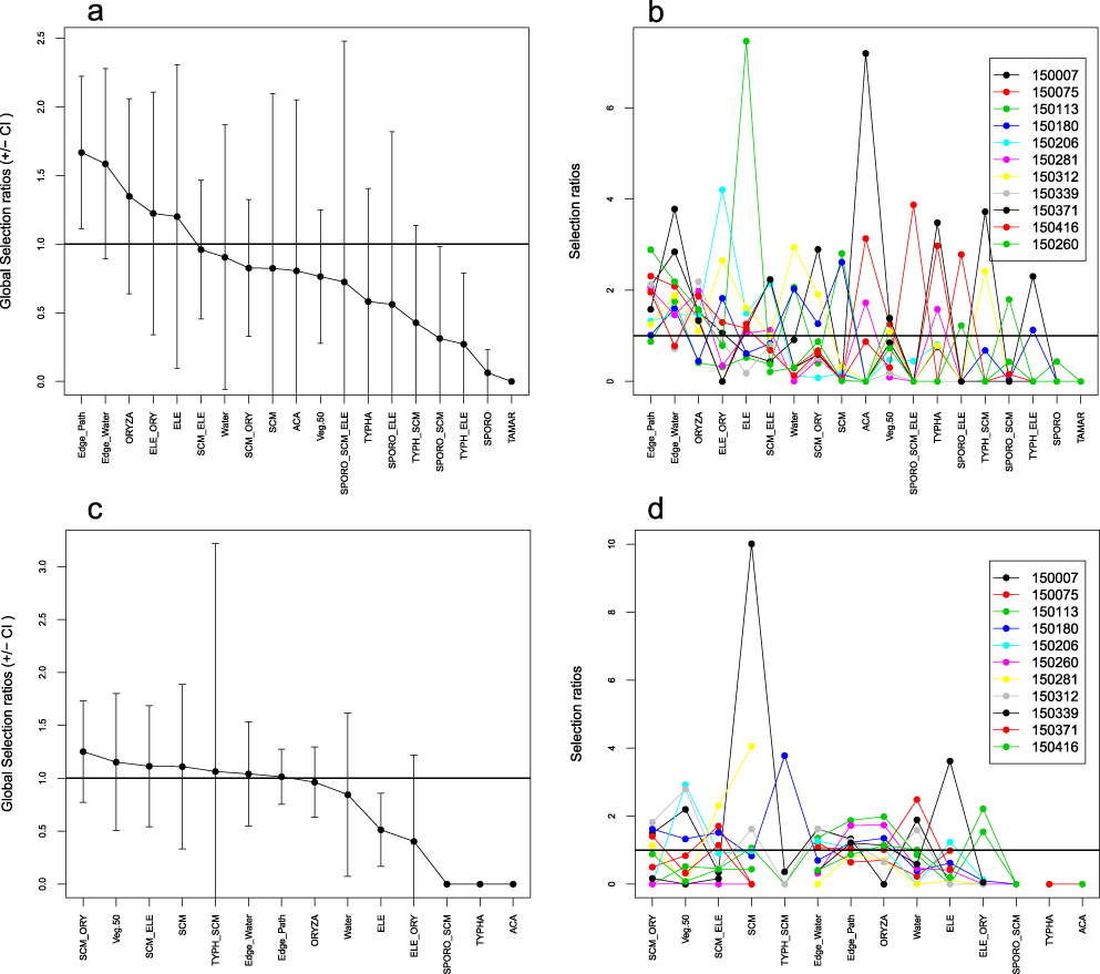
Figure 4. a & c) Global and b & d) individual Manly selection ratios (± SE) for Design II (a, b) and Design III (c,d) for six Baillon’s Crakes radio-tracked at study site GL. Ratios are significant if their 95% confidence intervals do not include 1; values >1 indicate selection, values <1 indicate avoidance.
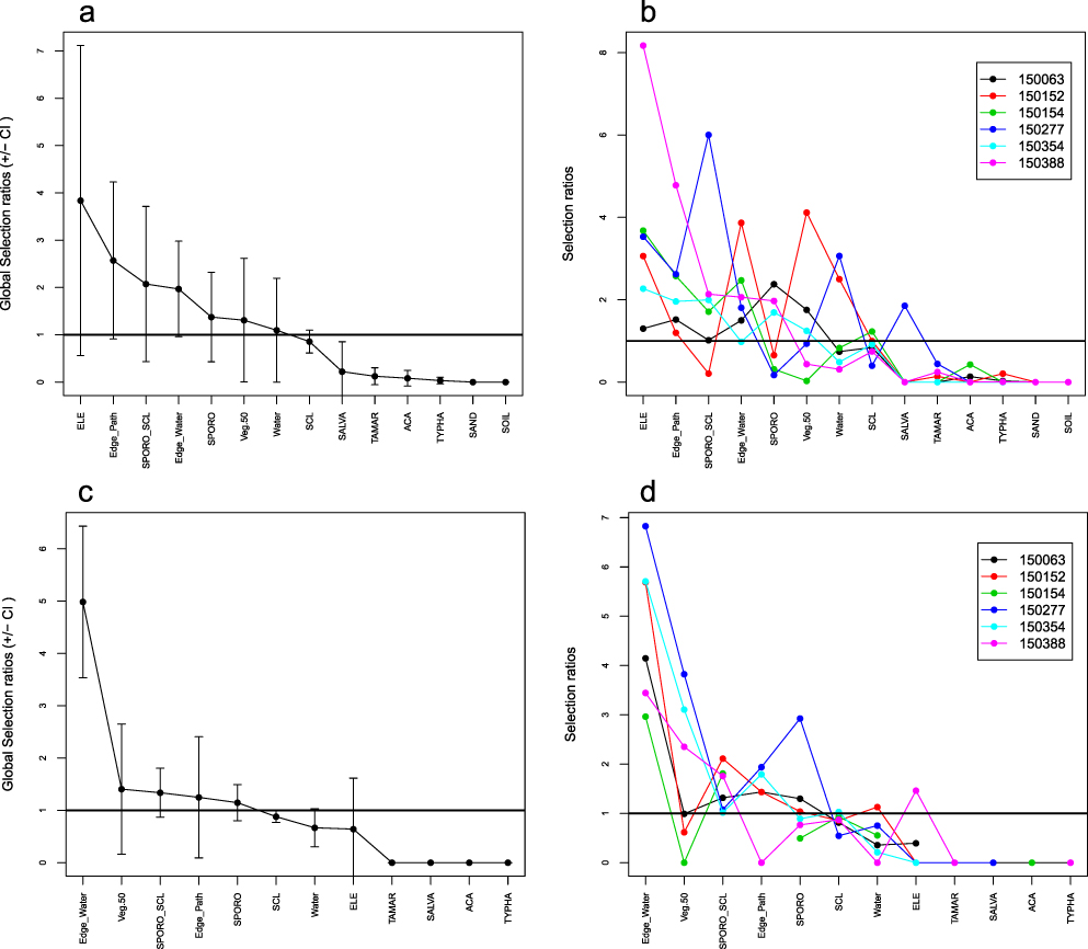
Figure 5. a & c) Global and b & d) individual Manly selection ratios (± SE) for Design II (a, b) and Design III (c,d) for eleven Baillon’s Crakes radio-tracked at study site TG. Ratios are significant if their 95% confidence intervals do not include 1; values >1 indicate selection, values <1 indicate avoidance.
Considering both use and availability of habitat parameters for each radio-tracked Baillon’s Crake individually (Design III) by comparing composition of land cover classes at the bird’s relocations with the overall composition within its respective 95% Kernel, only the global Manly selection ratio for Edge_water proved to be significantly positive for GL (Figure 4c). Overall, selection was highly variable across the radio-tracked individuals identifying no general preference for specific habitat parameters (Figures 4d, 5d).
Population level
The best models included four (logistic model) and five (Poisson model) habitat variables, respectively (Table 3a,b, Appendix S1). Thereby, edge structure of T. australis and O. longistaminata as well as S. littoralis stands affected probability of presence of Baillon’s Crakes positively, while it was negatively correlated to the occurrence of monotonous stands of T. australis (Table 3a). Density of Baillon’s Crakes was positively affected by edge structures of E. mutata and O. longistaminata. However, densities decreased when area of E. mutata, T. australis and S. maritimus increased (Table 3b). The cross-validation scores of the best models were 0.233 and 2.595 (logistic, Poisson), respectively. Cross-validated model prediction versus presence probability (Fig. 6a) and captures (Fig. 6b) revealed that both models could be used for relatively reliable predictions of presence/densities in comparable habitats.
Table 3. Standardized effect sizes (± SE) of the best models (logistic, Poisson).
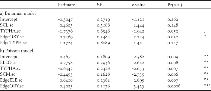

Figure 6. Cross-validated model predictions versus probability of presence (a) and captures (b). Grey dots indicate grouped mean values (and 95% credible interval). The black line indicates perfect fit. Mean values below the line indicate underestimation of presence probability/densities while values above the line show overestimation by the models.
Habitat suitability and population size estimate
We applied the logistic model to the land-cover raster data set obtained from the satellite picture (Tegetmeyer et al. Reference Tegetmeyer, Fricke and Seifert2014) and derived a map of probability of presence for Baillon’s Crakes in the Djoudj area (Figure 7). By using presence probability as a proxy of habitat suitability, the predicted area of potential Baillon’s Crake habitat with a probability >0.5 sums up to 9,516 ha (95% CI: 3,138–19,166 ha). Applying the Poisson model to the land-cover raster data set and summing predicted numbers of individuals for each raster cell, we obtained a potential population size of 10,714 Baillon’s Crakes in the study area. The 95% confidence interval ranged from 3,146 to 17,408 individuals.

Figure 7. Prediction of presence probability of the Baillon’s Crake within the Djoudj area.
Discussion
Home ranges
The extent of a home range might be governed by a multitude of different factors. Differences of home range sizes can be attributed to sex (Legare and Eddleman Reference Legare and Eddleman2001), age (Krüger et al. Reference Krüger, Reid and Amar2014) or body conditions (e.g. Harestad and Bunnel Reference Harestad and Bunnel1979). Home range size often negatively correlates with resource abundance (Village Reference Village1982, Glenn et al. Reference Glenn, Hansen and Anthony2004), leading to strong variation between habitat types (Conway et al. Reference Conway, Eddleman, Anderson and Hanebury1993, Rush et al. Reference Rush, Mordecai, Woodrey and Cooper2010). Furthermore, territories in the breeding season are often smaller than those established during the non-breeding season, as e.g. in the case of Clapper Rails Rallus longirostris which expand their home ranges from a median of 0.28 ha to several square kilometres after breeding (Eddleman and Conway Reference Eddleman, Conway, Poole and Gill1998, Cumbee et al. Reference Cumbee, Gaines, Mills, Garvin, Stephens, Novak and Brisbin2008).
With a mean size of 1.77 ha, the home range estimates for Baillon’s Crake in the Senegal River Delta are in the range of home range sizes inferred from radio-tracking reported for other small rallid species such as the Black Rail Laterallus jamaicensis (0.51–3.1 ha; Legare and Eddleman Reference Legare and Eddleman2001), Yellow Rail Coturnicops noveboracensis (1.2 ha, Bookhout and Stenzel Reference Bookhout and Stenzel1987) and Spotted Crake Porzana porzana (median 1.32 ha, Schäffer Reference Schäffer1999). We found the variability in home range size to be rather low compared to other studies (e.g. Spotted Crake 0.44–55.46 ha, Schäffer Reference Schäffer1999; King Rail Rallus elegans 0.8–32.8 ha, Pickens and King Reference Pickens and King2013). However, considering the short range of our transmitters of approximately 1,000 m, we might have missed longer movements of birds which would have increased home range sizes. Dispersal-like movements following the breeding season are generally poorly investigated in rallids but observed for Virginia Rail Rallus limicola and Sora Rail Porzana carolina (Johnson and Dinsmore Reference Johnson and Dinsmore1985) of which some individuals were found to start moving distances >500 m when chicks became independent. We can only speculate whether the abrupt loss of signals of four birds in GL and two birds in TG despite “favourable” water levels in the field season 2009/2010 (N. Seifert unpubl. data) can be interpreted as such short-range dispersal movements. Rapidly decreasing water levels of 0.5 cm*day-1 in the course of the season (Seifert et al. Reference Seifert, Koschkar and Schmitz Ornés2015) might have been a reason for birds to leave the study sites as hypothesised for four birds in TG (2009/2010) where home ranges were dry when the birds’ signal was lost. Other birds shifted their home ranges towards zones which were still inundated as indicated by southward (TG) and south-westward (GL) movements which corresponded to the respective relief in GL and TG (Franke Reference Franke2013, N. Seifert unpubl. data).
In general, interpretation of our data is complicated by the mostly unclear reproductive status of the radio-tracked birds. The breeding season in the Senegal River Delta starts in October and may last until January/March, depending on water levels in the PNOD and its vicinity (Seifert et al. Reference Seifert, Becker and Flade2012). Accordingly, within the period December–March, some birds might still be breeding while others have already completed reproduction. Furthermore, some Baillon’s Crakes might as well stem from distant breeding areas and use the Senegal River Delta as a non-breeding site (Seifert et al. Reference Seifert, Haase, Van Wilgenburg, Voigt and Schmitz Ornés2016). Accordingly, our data do not allow an explicit statement about the size of Baillon’s Crakes’ breeding home ranges but rather give an approximation possibly comprising breeding, post-breeding and potentially wintering home ranges. Certainly, longer observation periods would help e.g. to delineate possible core areas (frequently visited spots within the home range) and thus the deduction of the birds’ status.
Consistent for almost all radio-tracked individuals was the observation of longer distances between the location of capture and the first relocations after 48 h. Based on a very low recapture probability observed during our field seasons in the Senegal River Delta (total number of captured Baillon’s Crakes 2007–2013: 337 individuals, of which 15 individuals were recaptured within the same field season) and for other crake species in the Peene River valley, northeast Germany (A. Eilers, B. Herold, N. Seifert unpubl. data), we hypothesise that Baillon’s Crakes respond rather sensitively on disturbances such as capture. Besides the possibility that birds become trap-shy our data suggest that intrusions can lead to evasive movements, forcing the birds to abandon former and establish new home ranges. This behaviour should be taken into consideration for the design of studies investigating e.g. densities of rail species based on capture-recapture data.
Habitat selection
On the population level, our regression models confirmed that the occurrence of Baillon’s Crakes in the floodplains of the Senegal River delta is positively correlated to rather low and dense vegetation types such as S. littoralis while tall and rough-textured stands such as T. australis have an explicit negative effect both on abundance as well as presence probability. This finding is in accordance with previous observations of Baillon’s Crakes in European breeding grounds selecting for fine-stemmed vegetation and avoiding extensive reed-beds and cattail stands (Noll Reference Noll1924, Szabó Reference Szabó1970). Furthermore, Baillon’s Crakes were generally less abundant in vegetation dominated by species which do not provide adequate cover such as E. mutata and S. maritimus. While monospecific stands of E. mutata can form impenetrable and flat layers when plants collapse due to wind and decreasing water levels, S. maritimus grows more sporadically, often forming loose stands with poor cover, especially in lower depressions with high water levels (Tegetmeyer et al. Reference Tegetmeyer, Fricke and Seifert2014, N. Seifert unpubl. data).
Variables expressing heterogeneity in vegetation composition were included both in the logistic as well as Poisson model, revealing increasing presence probability and abundance with increasing edge length of patches of O. longistaminata as well as E. mutata and T. australis, respectively. All selected vegetation types have in common that transition between different specific patches is quite distinct. O. longistaminata often forms monospecific and very dense stands with its leaves forming a continuous overhead cover, resulting in well-defined edges at the transition to other bordering stands. The same effect is observed for small patches of E. mutata, especially when collapsed, while stands of T. australis interspersed into bulrush- and grass-dominated habitats indicate areas of rather sparse vegetation with a high proportion of open water and thus also distinct edge structures. The importance of edge structures in Baillon’s Crakes’ habitat selection was also reflected on the individual level, manifested in second order habitat selection by selective use of the land cover classes “path” and edge length of water bodies by radio-tracked birds in the study sites GL and TG.
Preferences for edges have been identified in several habitat selection studies of bird species inhabiting comparable habitats such as Aquatic Warbler Acrocephalus paludicola (Tanneberger Reference Tanneberger2008), Reed Warbler A. scirpaeus, Marsh Warbler A. palustris and Sedge Warbler A. schoenobaenus (Surmacki Reference Surmacki2005). Likewise, the composition of home ranges of King Rails revealed selection of microhabitat based on distance to open water and plant species richness (Pickens and King Reference Pickens and King2013) and studies of foraging behaviour of Clapper Rails indicated extensive use of emergent marsh edges (Clark and Lewis Reference Clark and Lewis1983, Zembal and Fancher Reference Zembal, Massey and Fancher1989, Rush et al. Reference Rush, Mordecai, Woodrey and Cooper2010). Most studies explain this pattern with a better food supply, as structural as well as micro-climatic conditions near edges are more favourable for many invertebrates (Voigts Reference Voigts1976, Kaminski and Prince Reference Kaminski and Prince1981) with e.g. dipterans being blown over the lower area and stopped in front of higher vegetation stands, while Odonata may use such boundaries for spatial guidance (Baldi and Kisbenedek Reference Baldi and Kisbenedek1999). Rehm and Baldassarre (Reference Rehm and Baldassarre2007) found especially the interface between vegetation and open water an important parameter explaining abundance of several marsh bird species such as Sora Rail and Virginia Rail as well as American Bittern Botaurus lentiginosus and Least Bittern Ixobrychus exilis. In contrast to the aforementioned studies, the authors consider the reduction of intraspecific competition is due to visual isolation of territorial birds by a spatially complex pattern of interspersed vegetation and water as the main reason promoting increased breeding densities.
In the two study sites GL and TG, invertebrate abundances especially of Brachycera, Coleoptera and Saltatoria were found to be significantly higher at vegetation edges (Seifert et al. Reference Seifert, Koschkar and Schmitz Ornés2015). Accordingly, it seems likely that food availability is an important factor for Baillon’s Crakes leading to disproportionate use of edge structures. It can also be speculated whether the smaller home range sizes found for TG are a response to higher heterogeneity (plant species richness, edge structures) of the study site, potentially providing higher food supplies. This would be comparable to Pickens and King (Reference Pickens and King2013) who found home ranges of Clapper Rails being smaller and movements significantly shorter when 95% kernels contained greater amounts of small, interspersed water bodies. However, based on our rather small sample size and the unclear reproductive status of radio-tracked birds, other underlying factors such as reduced intra-specific competition could not be investigated in this study and therefore cannot be excluded here.
Interestingly, in second order habitat selection, only E. mutata stands in GL were significantly selected among vegetation types by radio-tracked birds. Beside those patches providing invertebrate-rich edge structures, the plant fraction of Baillon’s Crakes’ diet was found to consist almost exclusively of seeds of E. mutata (Seifert et al. Reference Seifert, Koschkar and Schmitz Ornés2015), indicating that this plant species also provides an important component of the birds’ diet. Furthermore, fresh stalks of the plants may be used as nesting material as the majority of nests in GL were found in small patches of E. mutata (N. Seifert unpubl. data). As most individuals did not clearly select any other vegetation type, we hypothesise that in second order selection representing home ranges, structural characteristics of vegetation are generally more important for Baillon’s Crake habitat selection than plant species composition.
Third order habitat selection revealed rather low selection levels with only relocation of individuals at GL being disproportionally more associated with edges along water bodies. Apart from this, individual ratios showed on the one hand strong differences in selectivity between animals, resulting in wide confidence intervals and non-significant global selection ratios. On the other hand, ratios were distributed close to 1, indicating little difference in individual use and resource availability within the home ranges. Several explanations may account for this apparent lack of (consistent) selectivity. Firstly, in hierarchical selection analyses there may well be levels already too high to detect differences in usage and availability as major selection has already been made on a lower level (Johnson Reference Johnson1980, Thomas and Taylor 1990). Accordingly, the smallest scale in selection considered in this study might be below the smallest scale at which Baillon’s Crakes (in our study design) perceive and respond to habitat structure (Kotliar and Wiens Reference Kotliar and Wiens1990). Secondly, however, due to the rather low number of relocations obtained for most of the radio-tracked birds, we were not able to delineate core areas which could have revealed stronger patterns of selectivity within the home ranges by identifying and weighing repeated usage of certain habitat structures.
Furthermore, owing to its strong seasonal dynamics water level was not considered in our analyses, although this parameter is most probably of major importance and influences all levels of habitat selection of Baillon’s Crakes (B. Taylor pers. obs.). Especially in TG, where some areas of the study site fell dry in the course of the season, birds were forced to constrict their whereabouts to remaining patches which were still water-logged. Thus, availability of some habitat structures may have been more restricted than we were able to account for in our study design.
Habitat suitability and population size estimate
Based on our models, we predicted the extent of suitable habitat in the Djoudj area to comprise 9,516 ha (95% CI 3,138–19,166 ha). However, these numbers should rather be interpreted as a potential maximum extent, as water level could not be included in our models. In practice, water levels in the floodplains decrease from approximately mid-November on (Schwöppe et al. Reference Schwöppe, Terlutter and Willers1991), after the closure of sluices usually around mid-October (I. Diop in litt.). Thus, the effective size of suitable area diminishes in the course of the dry season until almost all shallowly inundated sites are dry by March (N. Seifert, C. Tegetmeyer pers. obs.). However, the gradual reduction of habitat size may not be linear as Baillon’s Crakes seem to prefer intermediate water levels from 10 to 30 cm (Taylor and Van Perlo Reference Taylor and Van Perlo1998, Franke Reference Franke2013, Seifert Reference Seifert2015) and some formerly deeply flooded sites in the centre of the National Park may become suitable rather late during the season while others are already completely dry by then.
Our population density model predicted a population size of 10,714 Baillon’s Crakes (95% CI 3,146–17,408) within the study area. Referring to the potential extent of suitable habitat, this would result in a density of 0.90–1.12 birds*ha-1 which is of the same magnitude as our home range size estimates with a mean of 1.77 ha suggests. Assuming that one home range comprises one breeding pair and does not overlap substantially with home ranges nearby, densities would constitute 0.88 birds*ha-1. Abundance data for Baillon’s Crakes both in breeding as well as non-breeding habitats are scarce with only Taylor (unpubl. data 1997 in Taylor and Van Perlo Reference Taylor and Van Perlo1998) reporting a minimum of 2 birds*ha-1 in a breeding site in South Africa and densities of 4 birds*ha-1 for non-breeding birds in Kenya. A sole observation of 41 birds*ha-1 indicates that the species can potentially occur in very high densities, at least outside the breeding season (Taylor and Van Perlo Reference Taylor and Van Perlo1998). Against this background our estimates seem rather low. However, data from study sites where birds were repeatedly captured during the field season indicate that densities vary clearly between sites and years (N. Seifert unpubl. data). Thus, Baillon’s Crakes are most probably not homogeneously distributed throughout the habitats in the Djoudj area. Furthermore, decreasing water levels may force the birds to gather in sites which are still inundated, leading to potentially increasing densities towards the end of the season.
In general, comparison of abundance data of rallid species might be futile as numbers are often reported to be highly variable. The population of Spotted Crakes in Biebrza Valley can differ by 90% (Schäffer Reference Schäffer1994) between years. Jenkins et al. (Reference Jenkins, Buckton and Ormerod1995) estimated the population density of Water Rails Rallus aquaticus to sum up to 14 birds*ha-1 while Brambilla and Rubolini (Reference Brambilla and Rubolini2004) inferred breeding densities of 1.85 birds*ha-1. As the controlling factor governing abundance of crakes is often specified to be water level (e.g. Koshelev Reference Koshelev and Tucker1994, Schäffer Reference Schäffer1999, Pickens and King Reference Pickens and King2013, B. Taylor pers. comm.), we assume that the size of the Baillon’s Crake population in the Djoudj area may also vary substantially between years owing to inter-annual differences in water regime, governed by factors such as meteorological conditions as well as the hydrological management of the PNOD.
Significance of the Djoudj and the Senegal River Delta
Owing to the species’ secretive behaviour and erratic occurrence, population estimates for Baillon’s Crake should be considered highly tentative and certainly erroneous. The official projection by BirdLife International (2015) assumes a global population size of 8,700–25,000 mature individuals, while some national population estimates are already up to 100,000 breeding pairs (e.g. China; Brazil Reference Brazil2009). For Africa, only a few population estimates exist with Taylor (Reference Taylor, Harrison, Allan, Underhill, Herremans, Tree, Parker and J. Brown1997) assuming the South African breeding population to consist of 5,400 breeding pairs, while Wetlands International (2016) extrapolate a total of 10,000–25,000 individuals for Eastern and Southern Africa including Madagascar. Accordingly, based on these strong uncertainties it is impossible to infer the proportion of the global (or at least African) population for which the Djoudj area might serve as habitat. However, with a potential of 9,500 ha of suitable wetlands, the PNOD and the Senegal River Delta might be of outstanding importance for African and possibly also European populations of the Baillon’s Crake. Although connectivity between European breeding sites and the Senegal River Delta has still not been fully understood, Seifert et al. (Reference Seifert, Haase, Van Wilgenburg, Voigt and Schmitz Ornés2016) suggested that the Djoudj area as well as adjacent floodplains in the delta (e.g. Diawling NP) could possibly be regarded as a source, playing an important role for the maintenance of the declining breeding populations in Europe.
Moreover, our discovery of a quite substantial but so far entirely overlooked population calls the reliability of recent population size assessments for Baillon’s Crake into question. Most of the national estimates are considered to be of medium or poor quality (BirdLife International 2015) or do not exist at all. It seems likely that there might be further important refuges whose relevance for the species are not yet sufficiently recognised. However, for a sound inference of e.g. the conservation status of the Baillon’s Crake it is indispensable to improve the baseline data both by intensification of field surveys and e.g. comprehensive modelling approaches to counteract the difficulties in recording this evasive species. Especially for West African wetlands such as the Inner Niger Delta, Mali, which are increasingly influenced and altered by agricultural utilisation and hydroelectric power production, further research is necessary to investigate potential occurrence of the species and enhance population estimates for the region.
Implications for habitat management
It is well established that habitats need to be sufficiently inundated as a prerequisite for the occurrence of Baillon’s Crake (Taylor and Van Perlo Reference Taylor and Van Perlo1998). Accordingly, providing appropriate water levels throughout the (breeding) season is the key measure in managing the species’ habitats. Therefore, water levels between 10 and 30 cm should be targeted as these levels allow a dense growth of the typical sedge or bulrush dominated vegetation. However, the establishment of monospecific stands should be avoided as diversity of both plant species and habitat structure increases the abundance of invertebrate food and thus habitat suitability. Small-scale structures such as open water bodies or bare soil, trampling paths and a mosaic of higher and lower vegetation can be generally achieved and maintained by a low-intensity livestock grazing scheme with e.g. wetland adapted cattle. In some habitats prone to succession, grazing also reduces the invasion of plant species with unfavourable growth structure such as Typha or Phragmites spp. and can prevent the shift of wetland margins into shrub communities. However, as cattle grazing in wetland habitats can be problematic due to increased risk of erosion through excessive trampling and overgrazing as documented for many African wetlands (e.g. Driver et al. 2011), intensity, length and timing of the grazing period need to be carefully managed. For some regions and habitats, controlled burning can be an alternative way to sustain favourable vegetation composition and structure (e.g. McWilliams et al. Reference McWilliams, Sloat, Toft and Hatch2007). At some latitudes, though, effects of burning have to be carefully considered as biomass from the previous year provides essential cover during the onset of the breeding season (T. Wulf, W. Heim pers. comm.).
Supplementary Material
To view supplementary material for this article, please visit https://doi.org/10.1017/S0959270917000077
Acknowledgements
We are very grateful to Peter Becker, Steffen Koschkar and Marco Thoma for tireless and irreplaceable assistance in the field. The team of the Station Biologique du PNOD, namely Colonel Ibrahima Diop, Talla Diop, Moussa Thiam, Pap NDiaye as well as Dah Diop, and Yalli Diop always made our stay a pure pleasure. We thank Melanie Mielke and Katharina Groba who contributed considerably by polygonizing aerial imagery. Fränzi Korner Nievergelt provided valuable statistical advice while Martin Haase and Birgit Schauer kindly improved the draft of the manuscript. Last but not least we thank Martin Flade and Barry Taylor for their careful and constructive review of our contribution. We are indebted to the Stresemann-Fond of the German Ornithologists’ Union (DO-G), the Evangelisches Studienwerk Villigst e.V. and the German Academic Exchange Service (DAAD) for financial support.


