
The Chairman (Mr P. Fulcher, F.I.A.): We are here to discuss the Ersatz Model Tests paper. James Sharpe is an independent consultant actuary focussing on the calibration of internal models and matching adjustment portfolios. His co-authors are as follows: Stuart Jarvis, who is an actuary working at an investment management firm. He works with clients on strategic asset allocation and portfolio construction. That involves building and maintaining asset liability models. Finally, Andrew Smith, who will not be making a presentation but will be available to participate in the discussion. He has had 30 years’ experience of stochastic modelling in insurance and pensions.
Our opener this evening is Parit Jakhria. He is the head of long-term investment strategy at Prudential. Within the Profession, he is a member of the Finance and Investment Board and chairs the research subcommittee of that board.
All four of the individuals are members of the cross-party Extreme Events Working Party, but this particular paper was written in their individual capacities.
The format for this evening is that I am going to ask Parit to give a brief introduction, then James and Stuart are going to give a PowerPoint presentation and talk to introduce the paper. Then we will throw the meeting open for some comments.
Mr P. C. Jakhria, F.I.A.: My intention is to give you a brief background to the paper to help illustrate why it is important to the actuarial and insurance industry.
Most insurers are quite complex. On the liabilities side, they might have details of millions of different policies and various different products, et cetera, which need to be summarised. On the asset side it could be even more complex because they would need to create a simplified model of the global asset markets.
We know that to have a perfect model of the world of asset markets the model would need to be, potentially, as big as the world itself. It may even be worse than this because you need the model to run faster than real time for the projection, so it needs to be significantly larger. Alternatively, you need to make simplifications and come up with a model that is not perfect.
In conclusion, you need a summarised version of the model. It does not stop there, unfortunately, because there are two other exogenous factors to extrapolate for which make this more challenging. Firstly, most life insurers require projection of the liabilities quite far into the future. For example, a deferred pension could take you out up to 50 years.
Secondly, the regulations ask you to extrapolate in terms of probability as well, because you need to come up with a one in 200 stress test across all of your sets of liabilities. This requires you to search the tails of the distribution of the approximate model.
If this was not enough, often the amount of data and the material with which you have to make your judgement on the model is quite sparse. So the ersatz model team are going to take you through what this means and how to create some robustness in terms of testing and making best use of the modelling reserves.
Mr S. J. Jarvis, F.I.A.: I am going to assume that most of you have read the paper. It is a fairly technical topic but we have tried to explore the philosophical issues that it raises. We think it raises some important questions about the way that we, as a profession, use models.
What we are going to do, initially, in presenting the paper is to give an overview. We will explain some of our terms, what we mean by ersatz models, and explain the kind of tests that we applied to these models, which is a philosophical question. James (Sharpe) is then going to dig into some of the results of the paper in a bit more detail. But he is going to be fairly brief about this as we are particularly keen to hear your views and perspectives.
What I hope that we can do with this paper is to help us, as a profession, to be more accepting of model fits that are not perfect. We are all members of the Extreme Events Working Party. Much of the work of that working party has been to challenge the idea that perfection even exists. We are operating here, if you like, in social science. It is a different environment to hard science. You are not trying to uncover physical law with statistics. Rather, models provide a means for us to impose some kind of degree of order on the reality which is often quite messy. We need to do that in order to help us, or to help our clients, to make decisions.
Firstly, and I guess that this is the question which many of you asked when you heard about this paper this evening, is: what is an ersatz model? Ersatz just means a substitute for the real thing. Ersatz coffee was produced during the Second World War at a time of coffee scarcity. Obviously, in an actuarial context, the scarcity is often around data. Data is often too scarce for us to say with any confidence what model really drives our claims process, our investment process, or whatever it may be.
So what we have to do is fit a model, which we call an ersatz model. However, we are more or less clearly aware that this model is merely an estimate. We then proceed to use it to take decisions. What we as users or supervisors of these models have to ask, or what the regulator will ask of us, is: how should we test whether the model has been fitted appropriately? Is it appropriate to the use to which we are putting it? Dealing with these questions is the main topic of the paper.
Let us start with a simple example which is in the paper. We have a brief history of recent claims. These are shown on the left-hand slide of Figure 1. We are probably interested in estimating average future claims, the variability in these claims, how these claims co-vary with other lines of business, and from a reserving perspective we will want to worry about how bad future claims might be. So, we are interested in the tail of outcomes. Ten data points do not give us a lot to go on and we naturally feel the need to build a model in order to be able to answer these, and other, questions.
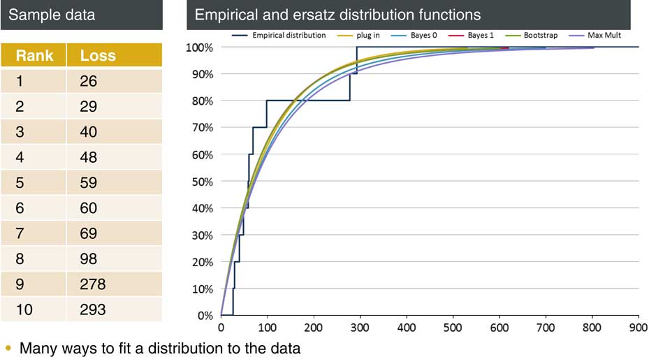
Figure 1 Example: predicting next year’s loss
Perhaps, by comparison with similar lines of business, we might have good reason to think that an exponential distribution provides a pretty good model of future claims. Or this might just be a social construct in that our predecessors have always used exponential models and we just follow in their footsteps. The mean of this data set is 100 so our simplest approach is just to take an exponential distribution with mean 100. This is the “plug-in” approach: we take some sample statistics, in this case just one, and set our model parameters to fit these exactly. This is the yellow curve. I suspect that this plug-in approach is by far the most common approach in real life situations today.
If we are worried about the fact that we have just pulled an exponential distribution out of the ether, we could simply use the empirical distribution which is the jagged line. This is unlikely to be very useful, we have no grounds for thinking that claims can never exceed 293, but perhaps it can be used to give us a qualitative or quantitative sense of whether our exponential assumption is questionable in this case.
A slightly different approach is a Bayesian one. We may be conscious that we are very uncertain about the mean of our exponential distribution and, while our data gives us reason for thinking that it might be near 100, it does not give us full confidence. So, we specify a prior distribution for the mean. For example, we may choose an inverse Gamma which keeps things analytically tractable. The net result is that we end up fitting a Pareto distribution to our data. Figure 1 shows a couple of choices here which are the blue and red lines. They are both improper priors which are scale-invariant and therefore might be called uninformative. Bayes 1 has the property that the estimates of the mean of the distribution are unbiased. Bayes 0 is a percentile-matching prior so the probability of exceeding the percentile estimate is exactly 1 minus the percentile for all percentile levels. We cannot have both at the same time but they are two potential routes that you might go down.
There are some other, more convoluted, approaches that we look at in the paper. One is the maximum multiplier method. This is perhaps a little esoteric. The method produces a fit based on the maximum rather than the average of our sample. We just focus on the maximum reading (293 in this case) and we fit a distribution based on that reading. We also look at a bootstrap method which is a way of smoothing the empirical distribution. We sample randomly from our original sample of 10, fit an exponential distribution each time and then average over these samples.
Each method gives you a way of at least making some prediction of the future. Which model you fit of course makes a difference, but it matters particularly in the tail. Things like mean and standard deviation, statements about roughly where the distribution is located and how wide it is, will usually be fairly clear even from a small amount of data. But statements about the thickness of the tail is are always much more dependent upon choices made by the modeller.
Figure 2 shows the previous chart blown up to show the top 25% and in particular the 99.5th percentile. The predictions for this percentile range from 530, for the plug-in method, to 803 for the maximum multiplier method.
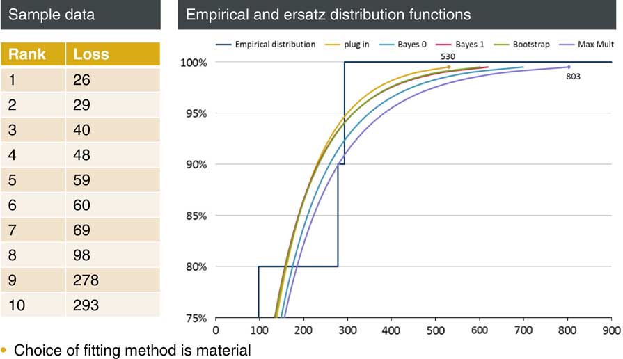
Figure 2 Model choice matters in the tail
So, how do we assess which of these five approaches is most appropriate to our needs?
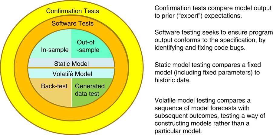
Figure 3 Testing: is a model good enough?
There are many tests we apply when investigating and checking models.
Very often we will apply a sort of “smell test” to the output. Does the output conform to what we would have expected? Is it consistent with what we have seen in other contexts? We might do a comparison, as in Figure 2, versus the empirical distribution. Does it seem to be broadly what the data is telling us?
These approaches depend on a degree of expertise, or at least experience, but are vulnerable to social groupthink. For example, perhaps we would never think of anything other than an exponential model because this is what everyone has always done for the last 50 years. Perhaps that is all that could be done 50 years ago when there was much less computing power.
Alternatively, we might check that the model is in conformity with its specification rather than our prior view. This is just a software test, seeking to capture any coding bugs.
We are interested here, though, in statistical tests we might apply, which are in the middle of Figure 3:
-
► An in-sample test will check that the realised data could have come from our fitted model.
-
► An out-of-sample model will seek to fit a model on one subset of data and then check the fit by comparing with a different subset. Cross-validation is one example of this; we are seeking to avoid overfitting.
Rather than just looking at a particular fit, an alternative testing approach is to focus on the methodology that was used to create this fit. If we apply this fit multiple times, then we can see how well the methodology performs. This also enables us to see what the model fitting will be able to achieve, and identify areas where we should be wary of relying on the model. Back testing is a classic example of this approach. If there is a long time series, fit a model at regular intervals based on the past and then test the future outcomes against this model. An alternative approach, which we advocate in this paper, is to test the fitting methodology by feeding it with generated data. We can then test the fitted, ersatz, model against the model used to generate the data, the true or reference model.
So that is the domain of our enquiry. We are often faced with a single past history. We want to say something about the range of uncertainty in the future. What we need is some kind of stochastic model.
If we knew what process drove the history we have seen, then we could use that to project forward to give us some sense about the range that we may see.
But we do not know that. We do not know the true model that produced the past history. So what we need to do is to fit a model, that is the ersatz model, and then we can use that fitted model to make ersatz projections.
As I have already said, in social science we do not have a physical constraint that determines the appropriate model. We are forced to simplify and fit a model that we then use to make real world decisions.
In my example we have an exponential distribution perhaps with a particular parameter. What we want to do is to generate a sample based on that parameter. We then fit a distribution, our ersatz distribution. We compare various statistics with that based on our true or reference distribution. You do this many times to see how well the fitting process performs in general.
In Figure 4 you can see how well this fitting process performs. We can compare the output from our ersatz model, the blue scenarios, against those we could generate from the reference model used to create the past.
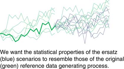
Figure 4 Is the ersatz model a good substitute?
Figure 5 shows, in summary, we have a reference model, for example, an exponential distribution with a particular parameter. We generate a sample from this reference model, fit an ersatz distribution and then compare various statistics of our fitted distribution against those for the reference model.
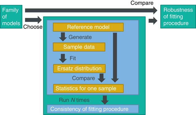
Figure 5 Tests on generated data
The results will depend on the particular sample that we happened to generate so we do this a large number of times and see how well our fitting procedure performs in general, that is, whether the fitted model is consistent, in some average sense to be determined, with the reference model.
Of course our fitting process might work well for this particular reference distribution but we often have to make a leap of faith in order to select a particular model. What if we had chosen a model that was slightly different or perhaps very different? Well, in this case we repeat the process for a family of models and again check whether the fitting process responds appropriately to different models. This is a test of robustness to the reference model. A fitting process might do fairly well on nearby models but lead to erratic behaviour if we stray too far. This knowledge will tell us what to beware of as we decide whether this fitting process is fit for our particular purpose. It will help us decide how confident we are about the kind of process that drives our data and what statistics of the ersatz distribution are important for our business decisions.
We have looked at a number of tests within the paper. There are two broad kinds of tests on which we focus: biased tests and percentile tests. With biased tests what you are doing is considering whether the particular parameter or level that is being estimated is consistent with the reference, or is there a systematic bias one way or the other.
This is particularly relevant in the context of things like Solvency II where you are looking to estimate a percentile. A different kind of test is where you estimate a percentile and estimate the likelihood of future outcomes falling above that percentile. If we make an estimate of the 99.5th percentile one would expect 0.5% of the future outcomes to fall above that. You might have a percentile that is unbiased but you will still have a probability of exceeding that percentile which is different. So there is need for a subtle awareness of the different roles of those two types of test which, I hope, comes through in the paper.
I am going to hand over to James (Sharpe) to talk about the results in more detail.
Mr J. A Sharpe, F.I.A.: In the next section of the presentation I am going to talk about some case studies that we have done where we have applied this approach in practice.
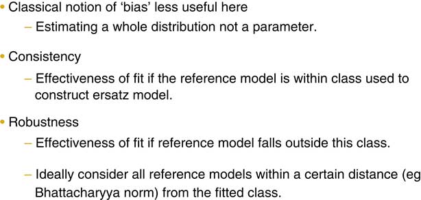
Figure 6 What makes a good fit?
But, before I do that, we need to consider what makes a good model fit? (Figure 6) There are a number of different tests which can be applied to a model when you fit it to a reference model. One of the classical statistical techniques is related to the notion of bias. Stuart (Jarvis) has just alluded to it. That is where the estimator for a parameter is unbiased.
In classical statistics this was always seen as something good at which to aim. Depending on the use of the model, it can indeed be a good aim. As actuaries, however, we are often trying to estimate the full distribution, so we might be in a position where we can tolerate some bias in exchange for some other features of the model which are better.
The second point is consistency. By consistency we mean our reference model and our ersatz model are from the same probability distribution so we are simulating some generated data from the reference model and then we fit each simulated data set to a model based on the same distribution. Then we test how well that is done.
The third point is robustness. The key point here occurs when the reference model is different from the ersatz fitted model. This is a great way of testing model error, as it shows the robustness of the fitting methodology to having the wrong model.
Figure 7 discusses consistency tests. As I mentioned, this is where the probability distribution from the reference model is the same as from the ersatz model.
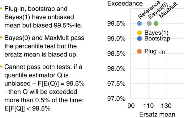
Figure 7 Consistency tests
This example is based on the first of our case studies which Stuart (Jarvis) has already discussed. As he mentioned, we have ten data points and our reference model is an exponential distribution.
The exponential distribution has a mean of 100 and we simulate ten data points from it. Then we fit five different models which are also based on the exponential distribution to the data set. We re-do that as many times as possible, say, 10,000 times or 100,000 times and then we can do any test we like on the output and work out how well the model fitting process is working.
You can see the plot on the right-hand side of the chart. This is showing the results of this approach of fitting five different exponential distributions to a reference model of an exponential distribution.
Along the X axis is the mean. Along the Y axis is the percentile exceedance test. We can see straight away that three of the model fitting methods have no bias. That is, they have given a good estimate of the mean.
To carry out the percentile exceedance test we fit our ersatz model and read off the 99.5th percentile, then we count how many exceptions we get above that from the reference model.
In our example, the Bayes 0 and the maximum multiple fitting methods have passed that test. They are also on the 99.5th level. The bootstrap method actually has about 1% of the real model above that. Thus it fails the exceedance test together with the Bayes 1 and the plug-in.
One important point that is discussed in more detail in the paper is that, in the case of an exponential, you cannot be both unbiased and pass the percentile exceedance test. So getting to the true reference model is not possible in the case of the exponential. Which approach is preferable depends on the purpose of your model fitting.
Figure 8 deals with robustness. This is something that probably worries many people who have come across financial time series. A particular issue is what happens if your data is from a fatter-generating process than the models that you are fitting to it. One of the things that we can do with this reference ersatz model testing approach is to test what happens if we do have that issue. In this case we have simulated returns from a Pareto distribution which has a fatter tail than the exponential distribution. The small points are the results from Figure 7. The larger points are the results from this test. You can again see that we have three model fitting methods that have no bias in estimating the mean. But all of them are failing the percentile exceedance test, which is not surprising because we are fitting with an exponential distribution against a reference model which has a fatter tail. The maximum multiple and the Bayes 0 give more robust model error. The MaxMult method gives more robust model error than the other fitting methods. It is an unusual way of fitting a distribution. Testing that model error is robust is not something that is commonly done.
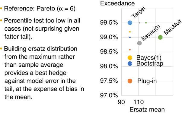
Figure 8 Robustness (1) fatter tail
Figure 9 is also about robustness. This time instead of testing for our reference model having fatter tails, we are testing for the data being auto correlated. That again is something that people fitting financial time series probably see quite often. If you are working with a data series you might not know for sure if there is auto correlation so what can you do about that? Often people just assume that there is no auto correlation, but here is a method where you can actually see what happens if there is auto correlation and our fitting method assumes that there is no auto correlation.
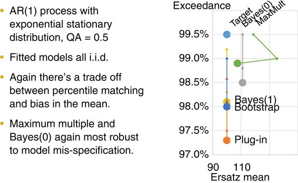
Figure 9 Robustness (2) auto correlation
On the right of the chart you can see the small points are showing the results of the previous two figures. The big points are showing the results from this test. We again have the unbiasedness of the Bayes 1, the bootstrap and the plug-in fitting methods. Again, the maximum multiple and the Bayes 0 could not perform much better on the model error robustness test.
In this case study of 10 years of general insurance (GI) loss data we were projecting just 1 year in the future. The issues we have considered become much more significant when you are projecting not just one but many years into the future. Thus we have repeated this same reference ersatz model fitting testing process with the Wilkie model, as in Figure 10. We have a reference model where we know what the Wilkie parameters are, we simulate some data from that and then we take an ersatz Wilkie model and we fit to that using a fitting method which is based on least squares parameter estimates. We do that many thousands of times and we can do whatever test we like on how well that fitting process is proceeding.
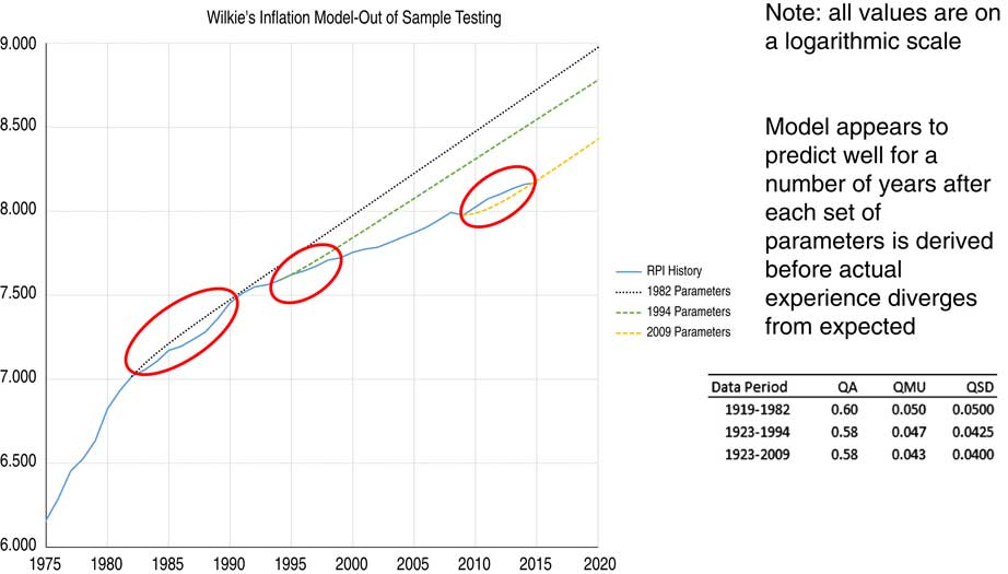
Figure 10 Example: Wilkie model for inflation
The least square parameter fitting method is intended to be unbiased. The results from this and the percentile exceedance test are shown in Figure 11.
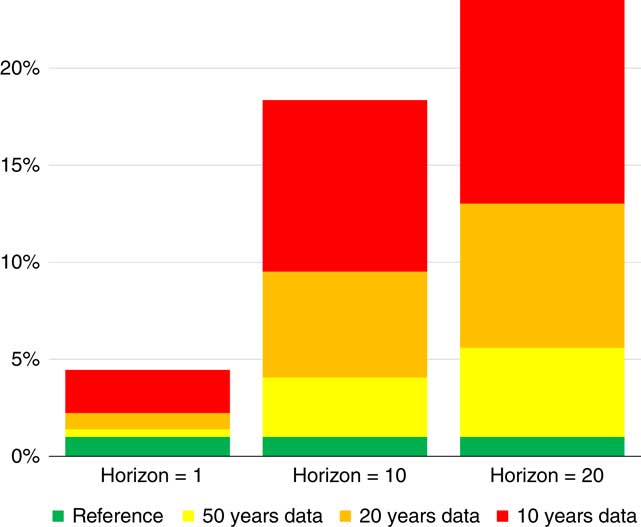
Figure 11 How often outcome < ersatz 1 percentile?
In the column on the left side we have simulated some historical data from the reference model. We are looking just one year in the future. We take the one percentile figure from our ersatz model and then we compare how often the true model is below that. If you had just 10 years of historical data and you are calibrating based on that, and you are looking 1 year in the future, you would find that about 4%–5% of the time the true model would be below that.
That issue is greatly enhanced when you are projecting further into the future. The worst case is shown in the bar on the right, when we have 10 years of historical data and we are projecting 20 years into the future. If you consider the 1 percentile figure from the ersatz distribution, you typically find that the reference model will be below that about a quarter of the time. There are generally more significant issues regarding the percentile exceedance test the further that you are projecting into the future.
One thing you can take away from our findings and perhaps put into practice relates to model validation. People with an internal model would have a calibration team producing an internal model and then often the validation team would check this methodology.
One approach to checking the methodology is to pick the calibration method that is being used and test it using this reference ersatz method. Typically a few different tests will be failed. As we saw previously, you cannot actually pass two tests at the same time: one will always be failed.
Typically, with validation, what happens is a number of different areas are investigated. Some sort of red, amber, green status is allocated and then, over time, you maybe work away at the reds and end up with just greens and perhaps a few ambers. We think that there are issues with the different fitting methods such that there will always be some red. That might not matter, depending on the purpose of the model. For example, if your purpose is to estimate the 99.5th or say a range of percentiles very accurately, like the 70th to the 90th, and it performs very well in that area, you might not be so worried if some of the parameters are biased.
One conclusion is that all models have issues so they are always wrong in some areas.
The second point is on testing versus generated data. I do not think many people are using the generated data testing approach in practice, but this is a strong validation testing method that can be used to supplement other methods such as testing empirical data and back testing.
We have also looked at model risk issues. This reference ersatz model fitting framework is a great way of understanding the model risk of your fitting methodology and also model and parameter uncertainty. We also have seen that the different model tests are conflicting. More details can be found in the associated full paper.
The Chairman: I will now hand over to the audience.
Mr J. Waters, F.I.A.: I was wondering if you had seen any companies doing anything like this in practice? It reminds me a little of the Lilliefors adjustment to the Kolmogorov–Smirnov Test, where you are testing for normality using the same sample that you used to fit the parameters of the normal distribution.
Mr A. D. Smith, H.F.I.A.: Yes, we have seen some of these things done. In general insurance, for example, there has been a lot of published work testing bootstrap methods for reserving variability, and there have been some disputes as to what those tests showed.
What we have managed to do is to articulate those tests in a more abstract sense that could also be applied to scenario generators and to life statistics. That was when we uncovered the fact that the tests conflicted. We think that that is a new result that had not previously been appreciated.
Probably the biggest risk facing most general insurers is catastrophe risk. However, we are not aware of this work having been done on the external catastrophe models used by general insurers. It is actually impossible for the insurers to apply these methods to the external models because they do not have the capability to recreate calibrations. So there is an institutional barrier to doing those tests. It does make you ask: what would you learn if you could do them and what can we do to break down that barrier?
On the question of the Lilliefors Test, this is exactly the sort of thing that we are proposing. If you had to derive the Lilliefors Test, you would need to simulate from historical data sets. You would need to fit your distribution by whatever method you liked, e.g., method of moments and you would need to calculate the Kolmogorov–Smirnov statistics.
Of course, if you are fitting normal distributions, you do not need to do that work because you can pick up a textbook and there are tables of critical values for the Lilliefors Test. But we do have situations where firms are, for example, fitting four parameter models to investment returns that could include skewness and kurtosis, and in those cases you have to do exactly what we have described. You have to re-run those methodologies to calculate the sampling behaviour of the Kolmogorov–Smirnov Test when you are fitting a four parameter model. So for that firms need to do, and are doing, precisely those calculations.
Mr A. J. Jeffery, F.I.A.: I thought that it might be interesting to share with you something that was presented at the longevity symposium last month. It was produced by Jon Palin, who has applied a synthetic set of data to modelling the cohort effect using the age period cohort (APC) model for longevity. The data that he applied had no cohort effect in it. The answer he obtained from data that had no cohort effect in it was quite a strong cohort effect.
The actual cohort effect in the period for which there was data was balanced out by other factors. But then as you project, you find the cohort effect predominating and coming to have an increasingly large effect.
What this is showing is that the APC model has a flaw in it. I colloquially would think of this as a hammer and it has gone looking for a nail and it has found it. This is a really important result which I think will be further disseminated over the next few months.
Mr G. J. Mehta, F.I.A.: How in practice do we make the choice of the reference model and its parameters in an objective way?
Mr Jarvis: There is, unfortunately, no easy answer to that question.
Mr Mehta: The reason I am asking this is to learn how to put these choices in perspective and communicate them to the different stakeholders. Let us say if I am not fitting a fat tail distribution and if I generate a reference model that has a fat tail distribution. As a calibrator you might be in difficulties if you do encounter problems of that nature.
Mr Jarvis: Ultimately, you need to make a choice or a number of choices. You need to make a choice about what broadcast models are going to be appropriate, and there is a social element embedded within that.
We have some ideas around the way you can make the process more model-free. For example, you may have some initial distribution and you look at all variations around that which are close in some probabilistic sense.
Ultimately, I think a lot of what we are exploring here is trying to give us tools, as modellers, to get a sense about how much that choice is driving what we are seeing. That is, to what extent would our confidence be different if we chose a different reference model or a different distribution?
Mr Smith: I will try to answer that and also to try to answer Tony (Jeffrey)’s previous point. There is an established statistical literature looking at robustness to which we have given some references.
There is a book by Huber & Ronchetti (Reference Huber and Ronchetti2009), to which we refer, discussing measures called influence functions which are partial derivatives of the output of a test with respect to the input factors.
There is also the concept of investigating robustness by looking at models within a neighbourhood of a particular model. That is discussed in the Hansen & Sargent (Reference Hansen and Sargent2008) book on robustness. Hansen was awarded a Nobel Prize in economics for his work in this area.
What we found was these are great theoretical concepts but they are incredibly difficult to implement numerically. They are also quite difficult to explain. So what we have done is something that is much simpler. We have said: suppose your best guess was the data came to an exponential distribution, what else might we consider instead? For example, there is a list of important distributions in the formulae and tables for actuarial examinations which might be good candidates. Given this, perhaps we might try a Pareto instead of an exponential and see how well it works.
In one sense this is arbitrary. But you are learning a lot and you are able to point out what happens if one model generated the data and we incorrectly fit another type of model.
To answer Tony (Jeffrey)’s point, you are right: one of the dangers of models is that the models spot patterns that are not there. One of the models we discuss in the paper, is the Wilkie model. One property of that model is a mean reversion effect, where after a year of good equity returns, you expect the next year to be worse, and after a year of bad returns you expect the next year to be better.
In the paper there is a reference, which Tom Wise and I put together, which shows when you take data from a random walk with no mean reversion and you put it through the Wilkie model calibration method quite a lot of the time you appear to see proof that there is mean reversion when you know there is not. As you say, that is a concern.
These sort of issues do not necessarily show that a model is flawed as it is just one particular test that has been failed. There are other tests which would be passed.
If you had a big list of tests, you could not pass them all at once. So the conclusion might not be that the model, say the APC model, is obviously poor.
The really useful information is to understand which test is really important for the application and recognise that some of the other tests will be failed.
Mr Jeffery: So if I can just come back, I did not actually say that the APC model was wrong or was useless. What I did say is it will look for a cohort. Now, we happen to know from other tests that the cohort exists. We are very certain that a cohort effect is working its way through the 1931 generation.
However, being alert to the danger of the model is the important thing. I suggest that is important not to fully concentrate on the statistical side but also look at the causality issues. You need to determine what the model is it actually saying and whether the results are generated by statistics.
I am not criticising the APC. I think that it is a very good model, but you have to be aware of its danger.
Mr Sharpe: Can I make a point on the choice of reference model? I think that when you are determining your ersatz model at the start you should do some exploratory data analysis and then you come up with a range of ersatz models you might use. In that process you are making some judgements, some assumptions, and on some of those certainly you might do some statistical tests to guide which approach to use. But in the presentation you showed what happens if those assumptions that you made are wrong. So those critical areas may be tested for, say, significant kurtosis.
Mr P. S. Langdon, F.I.A.: How does this process help if you have discontinuities in your models or the data-generating process?
Mr Smith: One of the models that is a particularly harsh reference model is what Taleb calls the Black Swan model, which is where your historical data has come from one process and recently, without you realising it, something changed and you are now in a different world.
It is quite clear that no statistical method is going to pass a test based on a Black Swan model. It is an inherent limitation of doing statistics that if you have a reference model where the past is divorced from the future, the statistics will not work. So to that extent there is not a lot that you can do apart from note that fact. You can of course check for more modest changes, for example, what would happen if there were a change in the rate of underlying inflation by 1% and you did not spot it, how would your model respond?
That is quite a common theme in the back testing literature for banking value at risk: how quickly does the model adapt to the high volatility regime? The answer is that it does not react immediately because if it did the model would be a so volatile as to be useless. If the model reacts too slowly then you will go well into the high volatility regime and potentially have huge numbers of big losses for which your model did not prepare you. That is one of the trade-offs.
Mr Jarvis: I work for an investment firm so we are always worried about what might happen to our portfolios, and we are always doing statistical tests, but we are also increasingly running scenarios, thinking about the kinds of thing that might happen to a portfolio or to a set of liabilities in the event of, say, a big spike in inflation, or Brexit, or whatever it may be.
Those are the kinds of things which I think we all need to understand about our businesses and portfolios, whatever they may be. There might be discontinuities but by running different scenarios we start to understand where are the risks and our exposures. It does not give you any probabilistic or statistical understanding, but, as a decision-maker, it gives you an understanding about where those risks sit.
Mr Jakhria: If you are forecasting, or looking one step ahead, it makes a lot of sense to get more of a handle on the tail. What slightly worries me is the situation where you project much further, say, 10, 20 or 30 years ahead. Does the number of permutations, in terms of how the model interacts with itself in terms of mean reversion or regime changes, simply make the family of models too big for it to be feasible to deal with mathematically?
Mr Smith: From a mathematical point of view, there is always some factor by which you could adjust your estimated standard deviation so that your model covers your desire for proportional outcomes. That might be a very large factor. I think that is because the further ahead you look, the more the uncertainty in the parameters you have fitted start to dominate those percentiles rather than the uncertainty that is captured within the model itself.
Those of us that were doing asset liability modelling in the 80s and 90s for pension schemes never really thought very hard about parameter error with the exception of David Wilkie, who was well before his time and published a solution in 1986 which was generally ignored.
It turns out that the biggest uncertainty was equity risk premium or something that practitioners were not actually modelling stochastically at all. That is definitely a cautionary tale and something which our testing methodology would pick up. The further ahead you are trying to project, the more it is that the uncertainty of your parameters comes to dominate those risks.
The Chairman: I guess for me a couple of the more interesting parts of the paper were about the cultural as well as the mathematical side of models. I guess the first one would be the whole name of the paper, ersatz modelling, starts with the point that all models are simplifications of reality. The question is: are they fit for purpose and are they correct?
A little anecdote here: in my first job in an investment bank, on my first day there, I went to watch a demonstration by a colleague of an asset liability model for insurance companies. He demonstrated it to the boss who said, with no irony whatsoever: “That model is great. And even better news, my car insurance is due for renewal tomorrow so I presume this will tell me to whom I should switch my premium”. This showed a genuine lack of understanding of the scope of the model.
Most of us, as actuaries, do modelling, so I ask these questions: Do we do a good enough job? Do the users of the models understand that our models are not perfect? Do boards and regulators, which have a habit of asking us to pass tests and jump through hoops, really understand?
Mr Jarvis: I think it is difficult to say whether people we are talking to understand the modelling that we do. I would say there is much more understanding than there was even 5 or 6 years ago. There is much more awareness that models can be a long way away from reality. I think the financial crisis has helped to make people aware of that, together with all the book writing that Nassim Taleb has done. There is a broad awareness that models are only a guide and not a version of the truth.
But it is always going to be the case that we, as modellers, understand much more about our models than the people to whom we present them. We will try our best to explain some of the deficiencies, but in a way it is perhaps contrary to our own interest to describe in too much detail what the issues are and too much what could go wrong.
Mr Smith: I would like to think that we can get to the point where we are much more comfortable discussing model limitations. At the moment, for some audiences, there can be a bit of a taboo about discussing model limitations. There is a fear that if you openly discuss the limitations of a model, that it will undermine confidence in that model and in the person who is presenting it.
We mention in the paper the example of a validation report that is all green. Naïvely you might think that is a sign of a good model whereas more likely it is a sign of self-deception.
There definitely is a need to be able to discuss those things more openly. At the moment, sometimes having discussions about model weaknesses is a bit like the interview question: what do you think is your greatest weakness? And you come up with something like: “Sometimes I work too hard”.
You look down lists of model limitations and you know perfectly well that the things that are listed as limitations are obviously both censored and things which are not really limitations at all.
There definitely is a cultural issue about being able to discuss model limitations openly. Some people have looked at modelling and said “this is an enormous amount of computation, it is an enormous amount of hassle and does it not show us things that we already know. Is it not obvious that if you are fitting models based on exponentials to something with fatter tails, you are going to underestimate the tails?”. For people in this room that probably is blindingly obvious. However, if the obviousness is sitting in your head and not committed to paper, somebody to whom it is not obvious will not be aware of it. Whereas, if you have a disciplined process of doing the testing and producing a result that cannot so easily be buried, there will be some progress on the model cultural aspect.
Mr Jakhria: It is interesting that the regulations ask you to use a single internal model to come up with a single estimate of the capital numbers. I do not know if that is manifested in the cultural bias you just discussed.
Mr Smith: I think many of us were involved in models long before Solvency II. And cultural biases were there, but it is perhaps concerning that they then became ingrained in regulations.
Mr J. C. T. Leigh, F.I.A.: I should like to return to the point that Andrew (Smith) made about discontinuities. I think it is a vital point when we are thinking about models. We obtain lots of data to use as the basis for the parameters of our model. We treat them as samples from a single probability distribution whereas, in fact, I suspect that in the real world, much of the time, each piece of data is a single sample from a different probability distribution.
With a bit of luck and with some continuity of business, that perhaps does not matter too much. But I think it is still a weakness and I think it manifests itself most greatly when you do have a major discontinuity.
You mentioned Brexit. But we know Brexit is going to happen and, when it does, we know there will be a big discontinuity. The problem is when we do not know there has been a big discontinuity, and I think that was probably a part of the problem with the financial crisis of a few years ago. The banks had built models to which, admittedly, there were quite a few theoretical objections but which made assumptions about the people taking out loans. These models were based on lending and default rates from people who had been given loans after they had had answers to various questions checked, and who had been checked for ability to repay and for the validity of their security, and so on.
That was changed within banks, probably without any policy change, to a system where, in effect, a loan was given to anyone who could fill in a form. That was not recognised in any of the models. The modellers probably would not have known how to reflect it and, indeed, quite possibly, the changes would not have happened if management had realised what was actually happening. You have there a major discontinuity in lending policy. That was what stymied all the models.
A different point that I would make is that I do feel somewhat uncomfortable with the idea that we can accept a model, or a formulation, that does well at a percentile level even though it may be biased at mean values. We are always being told that we must use our models for things other than capital projection if we are going to use them to set capital, and it is sometimes a bit of a struggle to persuade management to use the model for other things. If a model is only good at estimating, say, the 99.5th percentile, and is biased elsewhere, then I see that as quite a major problem in using models for other purposes.
The Chairman: I am tempted to say that that is a problem with the use test rather than a problem with the model but I will ask the authors if they wish to comment.
Mr Jarvis: I can only agree. Those of us who have been modelling for a while quickly learn that you build a model to do a particular job and you use a different model to do a different job. You are never going to have an all-singing, all-dancing model. You work out the need and you build a model using the best knowledge you have in that domain in order to make progress towards a decision.
The Chairman: One of the more fascinating mathematical results in the paper was that it essentially proved that was impossible to have a model satisfying all the potentially useful criteria.
Another point I took from the paper is that all models are wrong and a validation test that has a load of green on it is probably not a very good validation test. I wonder how people think their board or the regulator would react if they received a validation with a lot of red?
Mr Robinson: Insurers publish their 99.5th percentile to say how much capital they should hold. Do you think that it would also be valuable to publish a number that explained the uncertainty in that number? For example, you could specify a standard deviation of your required capital or percentile bounds in which you think your required capital lies.
Mr Smith: You are right to highlight that these numbers are very uncertain. Calculating a distribution of 99.5th percentiles is a difficult thing to do and is in itself subject to uncertainty. You have not really reduced the uncertainty by doing something even more uncertain around it. I think is an important thing to find ways of communicating the lack of confidence that any rational person would have on those models.
We gave the example of fitting a distribution and trying to come up with a one in 200 event based on ten data points. Some actuaries might say that is just an inherently stupid thing even to attempt to do. Unfortunately, it is something we are required to attempt to do, but that does not make it necessarily less stupid. What we have shown is you can say: “I have done this calculation and I have done it in order to pass these tests. Then here are the tests that it does not pass. You have set me a difficult task and I have done my best. This is how good my best is”.
I think it would be a step forward to explain what tests your method does not pass as well as the ones that it does pass.
I am sure that other people have views as to how you could communicate the uncertainty, the frailty, of the models that we use.
The Chairman: I think that it is worth reminding people again that all of the authors of the paper are members of the Extreme Events Working Party which was set up by the actuarial profession with the remit to outline what a one in 200 year event is for various stresses. It has probably been in operation for 7 or 8 years now. Its pretty immediate number one conclusion was that there is not an answer to what the one in 200 year event is for equity.
To be fair, this group has done as much as anyone to communicate the underlying uncertainty. The remit of the working party was to answer a stupid question, really.
Mr Jarvis: Yes, a stupid question that was asked by regulators. Regulators have been talking to actuaries for years and seem to have the opinion that “These guys are really clever. They will be able to test what this 99.5th percentile is”. In a way I suspect that, although we can blame the regulators, we probably should blame ourselves for some previous miscommunication.
Mr Sharpe: We did do some previous work a few years ago on the equity stress on value theory. We took the longest data series of non-overlapping data, something like 100 years data and fitted some extreme value distributions. Our best estimate for 99.50 was something like 40 something. A 95% confidence interval for that value was I think 20 something to 90 something. There was a huge level of uncertainty with the longest data set and using extreme value theory about the 99.5th estimate.
Mr Jakhria: I think that is assuming it all came from one distribution.
The Chairman: Something you touched on both in the paper and in the talk is that this methodology using the reference model probably does require a model where there is some robust or documented process for how it is actually calibrated.
You give the example in the paper of the Bank of England’s inflation forecast which is almost impossible to test, so who knows how the Bank would have reacted to slightly different data.
Is this lack of clarity a limitation of the methodology or is it actually highlighting an issue with models? If we frankly do not know how a model was calibrated, then that itself is quite a big red flag for a model.
Mr Smith: We have done a bit of thinking about this. You are right to say that the testing that we are proposing involves testing on computer-generated data. So if you wanted to apply that sort of test to the Bank of England you need to find 10,000 monetary policy committees who would be prepared to sit down and have their committee meeting based on test data and come up with their forecast. There probably are not enough skilled economists to populate all those committees and it would be quite expensive and quite laborious.
The way that I look at it is that there is a spectrum of estimates involving judgement. At one end you have technical statistical type models which you can easily test and at the other end of the spectrum you have political processes.
The Bank of England model is an overtly political process in that a system of voting within the monetary policy committee is used to come up with the numbers. I am not using “political” in a pejorative sense. It is just the nature of the process. Brexit is also a political process. If you want to check the answer for Brexit it is not possible to prove mathematically whether it was a sensible thing to have done. It is only possible to check issues such as: were the votes correctly counted? Did everybody who was entitled to vote have the opportunity to do so? Did anybody stuff ballot papers or break any other election rules? The checking of the political process involves checking the validation methodology and that the political process has been followed rather than that the outcome is correct.
The danger with some of the areas involving actuarial judgement is sometimes we see them as sitting in the middle. So we say that we cannot do political tests because it is a technical issue and we cannot do technical tests because it is a political issue. I would like to see a lot more clarity of understanding where the relevant boundaries lie.
To take another example, the ultimate forward rate under Solvency II extrapolates the yield curve. This was determined by a political process because there is a consultation paper from the regulator about how it is produced. The regulator does not produce consultation papers on entirely technical things. You do not expect to be able to produce a consultation paper on whether there are infinitely many prime numbers. That is a matter for mathematical proof.
We recognise political processes cannot be subject to ersatz model tests because the ersatz tests deal with mathematics.
What we need to do is to understand more of the processes where you have hybrids of technical and political elements and really try to be clear about where the boundary lies so the technical bits are thoroughly tested from a technical point of view and the political bits are thoroughly tested from a political point of view.
The Chairman: In a way that is a difficult issue if you look at it from the actuarial profession’s point of view. In some ways actuarial judgement has been what people regard as the added value of the actuary. At one end of the spectrum we are going to be replaced by politicians, at the other end of the spectrum we are going to be replaced by computers.
The actuary who sucks his or her pencil and makes a call is historically what this profession has aimed to produce. People come out at the other end of the exam process, which has quite an element of mystique, and are qualified to make judgements. I do not disagree with you but it feels quite a challenge to the way the profession is operated. The pensions world is probably going through this evolution a lot more slowly than the life world. The life world had to adapt to market consistency in a very short period of time. The pensions world has been dragged kicking and screaming in the same direction for the last 25–30 years. I think the non-life world probably still has an element of both approaches. There underwriters use their judgement and also very complicated actuarial modelling and additionally some fuzziness in between.
Mr Jakhria: As devil’s advocate, I would say that it is more a call to make your judgement more transparent. If we make it clear where we have made the judgements in terms of model structure, then it can be easier, as Andrew (Smith) says, to test the parts where we have not made judgements and then separately test the parts where we have made judgements. That is probably the only hope for the future of the profession.
Mr Jarvis: I am more on Parit (Jakhria)’s side than your side, Paul (Fulcher).
Mr Jarvis: What are we doing? We are helping to take decisions ultimately, decisions supported by models. The models do not give you the decisions. All kinds of things go into that process, as James (Sharpe) described it. You look at the data and you think about what kind of models would be sensible to fit. There is a choice that you have to make in terms of what modelling process you are going to apply.
Then there are various tests that you can apply to that process to think about whether it is going to lead you down a bad path and maybe have the kind of issues that you see with extrapolation, such as the cohort effect problems discussed earlier. There are all kinds of things which, as a user of the model, you need to make decisions about which require human judgement, for example, what kind of output you believe or do not believe.
You cannot put everything through a quantitative treadmill but you need to be clear about where the technical piece ends and where the actuarial judgement begins.
The Chairman: Solvency II has enshrined the concept of expert judgement. This is a formal concept that is explicitly labelled and has to be documented properly.
Have I created any thoughts in the audience about whether the actuarial profession has a future or not?
Mr Jakhria: There is a very interesting book by Martin Ford (Reference Ford2015) on robots and the threat of mass unemployment. I read that thinking and worrying about the future of actuaries. Based on the book, the only possible hope seems to be, as Stuart (Jarvis) mentioned earlier, collaboration. You have to collaborate to divide your problem into components that computers can solve more quickly than you and focus on components where one has to make a decision based on judgement. It is a fascinating book on the topic and I would encourage you to read it, perhaps when you are not already depressed with the current state of the world.
The Chairman: Regarding reading recommendations on that topic, there is another book which is more directly relevant called The Future of the Professions by father and sons called Susskind (Susskind & Susskind, Reference Susskind and Susskind2015). They are lawyers. Their conclusion is that there is not a future for professions. They do a very good job in the book of explaining what it is that a profession does, which is really having some specialist knowledge and therefore restricting access to certain activities. The need to have gone through professional exams would be a good example of restricting access, but also having trust is important. For example, doctors, actuaries and lawyers often claim that they can be trusted. People think professionals will make a decision objectively based on the data and knowledge that they have.
One of their points made in the book is that they still think that there is a future for the professions when it is almost life or death and someone is not prepared to trust a computer. They are more pessimistic when the activity is “number crunching”. We actuaries number crunch life and death.
Mrs E. J. Nicholson, F.I.A.: I am less worried about the threat to the actuarial profession because I see quite a lot happening around the expert judgement piece.
I am from a GI background, which probably means that I have quite a different perspective to people from other disciplines, but what I see as one of the key barriers to testing models at the moment is the resource constraints.
One of the things that I would be interested to understand is what thought you have given to prioritising statistical testing. Quite often when I am looking at models I see that a minimal amount of statistical testing is being done because there just is not time or resource or computing power to re-run the models over and over again on different bases.
The Chairman: I think it is acknowledged in the paper that this activity can be quite computationally intensive.
Mr Jarvis: The computing power that we all have available now is vast compared to what we would have imagined 5 or 10 years ago. I know that from my experience whenever we release a model from within my firm it is tested to the nth agree. It is tested in terms of what will it do and in terms of a whole series of backgrounds that we have within our firm. There is all kinds of unit testing taking place on models and this is a statistical kind of process. The models possibly would not pass some of the tests we are talking about today in the paper but at least there is an attempt to head towards that situation.
Mr Jakhria: I think the direction of travel of regulations and risk functions is also helping in that there are now dedicated model validation teams which I certainly do not remember 5 or 10 years ago. I do not recall the phrase “model validation” at the start of my career.
Chair: I think we can thank Solvency II for that development as well.
Mr Smith: There are lots of things that can go wrong with models and our paper is about statistical things that can go wrong with models. We have already had a comment from Paul (Fulcher) about whether the model will work if there was a sudden change in the environment. Julian (Leigh) gave the example of, essentially, a denaturing of the underlying process without people higher up being aware.
Those are all important things that could affect models. There is a sensible discussion to be had about what is proportionate for statistical testing as opposed to stress testing if the environment has changed or the data is not what we believe it to be. There is certainly a need for balance there.
The other point that still has to be worked out is how much of the statistical testing has to be done by the firm every time a model is used, and how much can be done in advance and written up in statistical textbooks.
We had the example earlier of the Lilliefors Test. The state of standard theory at the moment is that there is a Lilliefors test for normal distributions. There is not a similar published test for, say, hyperbolic or many other distributions. Firms who want to use those more complicated approaches have to build some of those tests. Presumably the time comes when that becomes textbook stuff. Just as whenever you take the average of a sample, you do not write out the proof that is an unbiased estimate of the mean. You can refer back to textbooks proving that is the case.
If it looks like an immensely complicated exercise, there may be some salvation, in that there are parts of the testing that can be done on behalf of larger groups by organisations specialising in those areas.
Mr Sharpe: It might be a good idea to have priorities in the testing. If there are some key uncertainties in the modelling it might be good practice to go ahead and test one of those uncertainties with quite high priority. I am putting forward the concept of basically testing what could go wrong if particular assumptions are incorrect. I would give that quite a high priority. It might not take too much computer power. I think running all the tests that we did in the paper is quite a lot of computational power. In practice, if you prioritised key areas, you would not be doing many different distributions all at once.
Mr Jarvis: To give you a sense of how unchallenging it is computationally, James (Sharpe) coded everything in one system, I coded everything in another, and Andrew (Smith) in a third, and we checked our results agreed.
The Chairman: I think what I take away from this excellent paper is all models are simplifications in reality. The question is not whether a model is correct or not, because it is not, it is a model. But it is whether it is fit for purpose.
There are various ways you can test a model. I think this new way the ersatz model team have suggested of using reference models and feeding data into your models to see how it works, is something which exists within the literature but has not been put down in the actuarial space before in a way that is standardised and consistent. Given the discussion that we have had it has also been addressed in a relatively practical way.
I think this is definitely an important contribution to the actuarial literature. I also liked the cultural discussion that it inspired. Frankly, if your model passes all the tests, you probably have not tested it properly. People need to understand the limitations of models. In reality, most of the examples the paper itself gives of model failures have probably been social and cultural. The Model Risk Working Party, which is a recent working party, also talks about social and cultural issues. Even just acknowledging the imperfections and the robustness of testing and allowing us to flush out what judgement is, what is political and what is statistical, itself changes cultures and therefore can help rid us of some of those issues.
So, I think this is a very important paper for the actuarial literature and I ask you to join me in thanking the authors.


 Open access