
The Chairman (Mr A. J. Clarkson, F.F.A.): Welcome to tonight’s discussion about the Aggregation and Simulation Techniques Working Party’s report – Simulation-based capital models: testing, justifying and communicating choices.
This paper covers copula and correlation assumptions and validation of the proxy model. Those are two of the areas that I find the hardest to validate when validating an internal model. In particular, how do you assess whether the fit of the proxy model is good enough when you do not know the right answer; how do you assess whether it matters whether there is a large difference in results from proxy and full models for one simulation if the simulation reflects risks that are not large for the company; how do you judge how many out-of-sample tests to run to compare results from the proxy and full models?
I should like to introduce David Stevenson and Steven Oram, who are members of the working party and will introduce the paper.
David was born and went to school in Thurso, which happens to be the birthplace of the first President of the Institute of Actuaries. He has a BSc from the University of Edinburgh and an MSc, PhD from the University of Warwick in Mathematics. He worked for Standard Life for over 20 years, including 4 in Frankfurt. His first experience in applying statistics in practice was a summer job as an undergraduate modelling the failure of fuel pins in a fast reactor core.
Steven graduated from the University of Dundee in 2007 with a BSc in Mathematics. Since then he has worked for Standard Life in a variety of roles, currently in capital and risk management.
Dr D. Stevenson, F.F.A.: I want initially to give a brief overview of the working party and some background to its work before I move on to copulas, particularly the issue of selecting correlations while allowing for tail dependence. I should like to go through a worked example of one of the techniques that we describe in the paper. Then I will hand over to Steven, who will say some words on the proxy models.
We have been seeing increasing sophistication in capital models. This has been partly motivated by Solvency II, which has the requirement to produce a full probability distribution forecast. There is also a requirement to justify assumptions on an empirical basis as well as all the statistical quality standards, documentation standards and validation requirements.
At least for those firms who have been seeking internal model approval, this has led to more sophisticated aggregation techniques, using simulation-type models and proxy functions, moving away from the correlation matrix approach, which was quite common in the former individual capital adequacy standards (ICAS) regime.
With that background of quality standards and validation requirements there is also the increasing scrutiny of the assumptions that go into this work by the stakeholders that are responsible for the quality of the internal model and meeting the standards, and the model validators themselves.
As a working party, our remit was to look into the different techniques that could be used, how actuaries could choose between the approaches and how those approaches could be validated, and the results of that validation communicated to stakeholders. We were not being asked to look at the relative technical merits of specific techniques. That was not our main focus.
We have produced a survey of the current practices in use by UK life insurers with internal models and some examples of how these approaches can be tested and the outcomes communicated.
Our focus has been on the copula and proxy model approach because that is the most widespread approach in the internal models that we understand have been approved to date. We hope that this will provide a useful reference document for actuaries who are working on internal models, and perhaps those who are going to submit internal model applications in future. We are not claiming that it is an absolutely foolproof and comprehensive toolkit. It has been based on information that we have been able to collect.
We stress that you should use the techniques that are appropriate to your own circumstances. Not necessarily every technique that is described in the paper will be appropriate.
To set the background, you have marginal risk distributions. These are distributions that describe how your marginal distributions behave. We also have a dependency structure, a copula, which tells you how to glue these things together in a way that reflects the dependency structure that you assume. Those two things give you a way of simulating from a multivariate distribution of those risk factors. You then have a proxy model, which is a way of describing how your balance sheet behaves under each of those shocks. You get a movement of own funds; you rank the movement of own funds and, at least for the purposes of Solvency II, you pick out the 99.5th percentile loss from that, and that is your solvency capital requirement (SCR). That is the basic idea.
I am just going to give a brief reminder of what is a copula; that is, the Gaussian or Student’s t copula. That definition will then be used in the example, which is one approach to calibrating the correlations of a Gaussian copula.
A copula, briefly, is a multivariate distribution with uniform marginals. Fundamentally, it is a recipe for gluing together the marginal distributions that you have defined in a way that reflects the underlying dependency structure.
If you can simulate from the copula, you can get a value that lies between 0 and 1 for each risk factor, then project that down onto the range of the marginal distribution, then project that back for the value of the marginal distribution to which that corresponds. Do that for every component of the copula. You will get a vector. In other words, you have a way of simulating from the multivariate distribution. That is basically what a copula is doing.
Most life companies that have had their internal models approved to date are using the Gaussian copula, the copula underlying the multivariate distribution; but there is a significant minority using a Student’s t copula.
That choice has been influenced by a number of factors. One is the balance between the transparency and complexity of the copula. How easy is it to explain it to your stakeholders? Do you want continuity with the correlation matrix approach under ICAS? Do you have a preference on whether to allow for tail dependence explicitly or implicitly? A t copula makes an explicit allowance for tail dependence.
The scarcity of data to support more complex models is another factor. Calibration does rely primarily on expert judgement, given the lack of data or even an absence of data in some cases. Do you want to go for a more complex model, which is difficult to justify, or do you use a simpler model and accept its limitations, but come up with a calibration that you can believe in, or at least that you can sufficiently rely on?
Underlying both of these copulas is a correlation matrix. The t copula has an additional parameter, the degrees of freedom parameter, which acts to control tail dependence. The Gaussian copula has zero tail dependence. The t copula has non-zero tail dependence.
The typical situation is that data is scarce or even non-existent. Data typically exists only for market risk factors, whose uses are limited. It may not contain sufficient information about extreme events. If you look at the data over different time periods, those may suggest different values for the correlations. So it is essential to supplement the data with an expert judgement overlay. If there is no data then you are forced to use expert judgement and to think about causal effects: what happens if one risk factor moves? What does it do to the other? What are the underlying risk drivers? Is there a common risk factor that underlies both of them and therefore increases the tendency of a large movement in one meaning a large movement in another?
Your own views on tail dependence and your own risk profile may affect which side of prudence on which you tend to err. If your balance sheet is sensitive to a particular assumption, or your capital requirements are sensitive to it, you are more likely to want to pay attention to the rationale underlying it.
Internal consistency of assumptions and benchmarking against other companies in the industry, if you are an outlier, will affect expert judgement.
Now I want to introduce the concept of the coefficient of finite tail dependence. This is looking at conditional probabilities. You are looking at the probability that if one risk factor exceeds its quantile, then the other risk factor will exceed its quantile. That is the coefficient of upper tail dependence, and there is a similar definition for lower tail dependence, as we see in Figure 1.
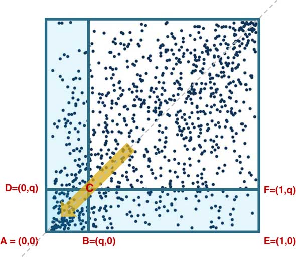
Figure 1 Coefficients of finite tail dependence
The coefficient of lower tail dependence is, broadly, for a given value of q, the probability that is contained in the little square divided by the probability that is contained in the rectangle. It does not matter which rectangle you choose. They both have the same probability.
I have used a slightly different definition to the usual one. With the copulas we are looking at, if you replace q by 1−q, the usual definition, these two functions coincide in the graphs. You can come up with empirical versions of these by taking the number of points that lie in the little square and the number of points that lie in the rectangle, and divide one by the other.
How do these look in practice? Conditional probabilities for a Gaussian model increase as you increase the correlation matrix. They also tend to 0 as the quantiles tend to 1. That reflects the lack of tail dependence within the Gaussian copula. For the t copula, we have, for example, one with the same correlations but with 5 and 10 degrees of freedom. What you see is that the conditional probabilities in the tail increase as the degrees of freedom decrease, and for the t copula they no longer tend to zero. They tend to a non-zero value.
Tail dependence is important because the probability of simultaneous extreme values in two or more risk factors depends on the presence of tail dependence. For example, we have a Gaussian copula with a 50% correlation assumption. Simply by moving to a t copula with the same correlation assumption but with 5 degrees of freedom, you effectively double the probability of the two risk factors, exceeding the 99 percentile at the same time.
If you are looking at extreme events, as you are for calculating capital requirements, the presence of tail dependence is something that you have to think about.
Those companies that have used the Gaussian copula, which does not include an explicit tail dependence, have tended to adjust the correlation assumptions in some way to compensate for this effect. I will come onto an example of one of these ways later.
The data that we have looked at is a set of equity credits, credit spread and interest rate risk factors from the end of 1996 to the end of 2014. That was 216 monthly movements in total. There is some significant correlation with equity credit. There is probably some tail behaviour as well.
Looking at different time periods, Figure 2 shows the Spearman’s rank correlation from the date on the x axis to the last date of the period (31 December 2014).
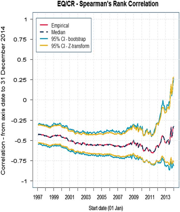
Figure 2 Spearman’s rank correlation; CI, confidence interval
As you can see, the correlation here does depend on time. We have plotted a 95% confidence interval around the central value, and if you look at the whole period the correlation is probably about −45% and maybe broadly a 10%–15% band either side of that for the confidence interval.
That might be helpful in informing a best estimate of what the correlation would be. Another technique that is sometimes used is to look at rolling correlations over shorter time periods.
In Figure 3 we have charted equity and credits over a window of 24 months, a rolling 24 months, and you can see from the chart that the correlation reached about minus 75% after the financial crisis in 2008–2009.
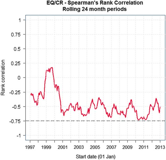
Figure 3 Spearman’s rank correlation over rolling 24 month periods. EQ/CR = equity values/corporate bond spreads
Another option would be to use statistical fitting techniques. There are a couple of variants. One is a method of moments, where you calculate the statistics from the sample data and you choose the parameters of your model to match them. For example, the Spearman’s inverse techniques can be used here, although if you have a t copula they do not solve it for the degrees of freedom. You have to estimate those using maximum likelihood.
The other statistical fitting technique is called maximum pseudo-likelihood. That is where you normalise the observations by dividing the ranks by N+1, where N is your number of observations. That gives you a result that lies strictly between 0 and 1. You evaluate the copula density function at those observations and form the likelihood function and optimise that in the usual way. There are standard packages, such as R, which do that. You can apply that to the data for periods of risk.
The key point to take away from this is if you are looking at the Gaussian or the t copula there is a relatively small change in the correlation assumption. For equity credit the degree of freedom parameter is quite small, which is possibly an indicator of some strong tail dependence, which you might want to look at further.
I want to go on to an example of one of the techniques in the paper which, if you have chosen to use a Gaussian copula, you might then use to inform how much you want to add on to your best estimate view of a correlation to allow for the tail dependence that is present.
This is based on some joint work with Stephen Makin but it goes back to ideas that were presented in a paper by Gary Venter in 2003.
There are other techniques available. This is just one of them. For example, with a t copula there is a technique that is based on matching higher rank invariants such as arachnitude, and that has been described in a paper by Shaw, Smith and Spivak in 2010.
How does this approach work? You take your data and plot the empirical coefficients of tail dependence, the empirical conditional probabilities that were described earlier. I have multiplied the equity returns in this example by −1 so we are looking at the tails where equity values fall and credit spreads increase, or equity values rise and credit spreads reduce.
There is some evidence of asymmetry. That might suggest that the Gaussian copula is, perhaps, not entirely appropriate. You then have on top of that the coefficient of the finite tail dependence for your chosen model. In this case it is the Gaussian model. I have used a correlation assumption of 50% here because that was roughly what came out of the likelihood estimation.
The line drops towards 0 and falls short of the tails. You can draw a confidence interval around that. I have used bootstrapping techniques. The bootstrapping is basically 5,000 simulations of 216 observations from a Gaussian copula with the chosen correlation assumption. If you find that values tend to lie outside that confidence interval, then that may be an indicator that that fit is not so good.
You can play around with this. You could change the assumptions that you put in. Moving the correlation assumptions to 60%, the line moves up. The confidence interval moves up as well. If you have a rough idea of where your base scenario is, the scenario that gives rise to your SCR, and if you have an idea of the direction of the risks to which you are exposed, you can play around with the charts and form a judgement on which correlation assumption you think best reflects the point in the tail where you are at with where you want to be.
In this case, if you were exposed to credit spreads up and equity returns down, and you have a scenario of maybe between the 90th and 95th percentile, then a correlation of the order of 70% might be okay. 70% seems broadly in the range in the tail.
Note that that results in adding on 20 percentage points to what you thought was a best estimate correlation, and that is well in excess of the confidence interval that you may have chosen based on the previous chart. So do not rely on confidence intervals alone. It is the conditional probabilities that you have to worry about.
Even then you still have sparse data in the tail. Once you have used these techniques, you have to think about the other factors that I mentioned earlier and overlay this with expert judgement in order to come up with your final view on the correlation assumptions.
There are some strengths and limitations of this approach. The key strength is that it is highly visual. You can place the charts in front of people and have a conversation about them. It is relatively straightforward for a Gaussian copula.
However, it does not generalise easily to other copulas. You still have to overlay it with expert judgement. It only looks along the 45° ray – that is, you are assuming the same percentile for both risks. You could try to broaden that by looking at ratios; instead of using the little square, you could use the little rectangle. But that is perhaps overly complex.
Mr S. Oram, F.F.A.: A proxy model is a model of the results produced by the full actuarial model suite, which is itself a model of reality. Proxy models were first used to partner copulas in simulation-based aggregation methods for calculations of capital requirements, an example of which is the Solvency II SCR. Here a copula is used to generate thousands – or potentially millions – of scenarios. The proxy model can then be used to calculate the balance sheet impact of each scenario quickly, which would not be possible using full models with current technology. Then the outputs are ranked and the SCR can be read off as the one-in-200 event.
Proxy models have since been extended to other uses, such as solvency monitoring. The key stages in building and using a proxy model are: design, which takes place upfront with periodic reviews; calibration, or, in other words, fitting the proxy model; and validation, which is testing how well fitted it is. Calibration and validation may be performed within the reporting cycle, but some firms seek to do elements of these off-cycle in order to meet reporting timescales.
There are many technical choices in the design and calibration of the proxy model, which we touch on in the paper, but the key focus is validation or how good is the proxy model at replicating the results of the full model, as that is what stakeholders will be interested in.
It is key that the validation takes into account the uses of the proxy model. So, for example, it will likely be used to calculate aggregate capital requirements such as the SCR, which is based on the results of thousands and millions of scenarios, as described previously. It will also be used to estimate balance sheet impacts based on evaluating individual scenarios in the proxy model following month-to-month or even day-to-day market movements. Each use requires the proxy model to be well fitted at different points of the probability distribution forecast. Typically scenarios that will be used to estimate the balance sheet response to short-term market movements will not be the same as those that affect the SCR. The consequence of the fitting errors will be different for each purpose, too.
It is therefore important to take into account the use of models when forming validation. Validation should also tell us something about the proxy model fit. It should be possible to investigate any issues by identifying which parts of the model are responsible for the errors observed, and to provide information for future refinements. It is vital that validation meets the needs of stakeholders, and that it provides clear information on the performance of the proxy model and draws clear conclusions on suitability for use. Finally, it must be practical to perform within the timescales required for reporting results.
A key type of validation is out-of-sample testing. Here a firm runs the same scenarios through its proxy model and full actuarial model suite, which are also known as “heavy models”, in order to compare results. Graphical displays of results, such as a scatter plot, can be informative. These can help to show at a glance how the proxy model performs at different points of the loss distribution, and can highlight issues that may be missed by summary statistics alone.
Here a perfect fit is effected by points in the 45° line, indicating that the proxy model and full model give the same results per scenario. Points on either side of the line indicate mis-statements, and it is good practice to consider the users of charts like this when creating them and to make it clear whether the proxy model is understating or overstating results.
Examination of the chart can indicate fitting issues such as clear outliers. We can investigate these to determine if there is a genuine error or a testing error. If it is a genuine error, it may not give cause for concern. For example, if it is a single point that occurs at a particular extreme combination of risks. However, a firm will want to know if it is indicative of a more systematic issue.
An example of a possible systematic issue is that losses are overstated in the region of the origin. This can affect the ability of the proxy model to accurately reflect short-term movements, such as those required for balance sheet estimation or for solvency monitoring. A firm would potentially want to look into these further, depending on the materiality.
A firm will aim to use its out-of-sample testing and other validation to answer two questions. First, is the model suitable for use? The answer may differ for different purposes. Second, can the model be improved either within the current cycle or in future?
We note that summary statistics can be informative but should not be the only source of information. Statistics alone will rarely diagnose a fitting issue.
Given tight timescales, tolerances can be invaluable in making objective decisions quickly, identifying areas which require further investigation. However, if these investigations do identify a limitation in proxy model fit during the reporting cycle, it is unlikely that a firm will have the opportunity to perform additional modelling to rectify it.
As a consequence, firms have adopted methods which use the results of out-of-sample testing to refine the proxy model calibration. We have outlined a number of such methods in the paper.
Ultimately, proxy models add an additional layer of approximation to the reported results and a firm’s validation can be used to understand and communicate the potential error around the true result which is caused by the proxy model.
I have touched on a number of considerations for validating proxy models. It is worth drawing on a key point of proxy modelling which is that errors are expected but bias and trends in errors are not. Validation should therefore focus on identifying these issues and provide output that enables stakeholders to gauge the potential impact on the end results. Visual inspection can be valuable in performing validation and as a communication tool.
The Chairman: I should like to introduce Jonathan Pears who will open the discussion. Jonathan is chief actuary at Standard Life.
Mr J. R. Pears, F.F.A. (opening the discussion): I found the paper successfully deals with some quite technical areas and diving down into them while remaining quite accessible and relevant. I also found that it provides practical advice for those trying to do this type of modelling and I am sure it will be a useful reference, having collected many techniques together.
The paper addresses a number of important themes. As the authors point out, the choice of the model and assumptions on dependency structure and the approach to aggregation can have big financial impacts and therefore potentially drive different action.
If you go back to the old approach in the individual capital adequacy of looking at individual risk factors, applying correlation and then maybe adjusting to come up with an answer, probably the biggest single number on the capital balance sheet was the diversification. Looking back to that, the amount of explanation of the judgements involved was probably relatively low compared with the significant impact that it has.
Given the limited data and the questions of the relevance of historic data, there is necessarily a significant degree of judgement in the choices being made here. Therefore, the communication of those judgements, the limitations and the consequences of using alternative approaches is important. But it is far from easy. I think that the paper addresses these issues well.
The first theme I will touch on, which is common to two sections of the paper – the section on dependency and the section on proxy modelling – is that of the high degree of judgement that is required in any model that is trying to approximate reality. The authors bring out, among other things, the scarcity of relevant data and features of the data that change over time. If you look at the work on escalating correlations, you will find in some periods they can be positive, in other periods negative.
There is a need for the model to be forward-looking and yet it is using historical data. It needs to be relevant to the current environment post-referendum rather than the past. The reliance that can be placed on past data is inevitably limited.
Models that fit well in some parts of the distribution may be a poor fit in others. That requires choices that are related to the use to which the model is put.
Another point that is brought out well is that the more features that the model tries to explain, the more relevant data is needed. Therefore, there is the potential risk of spurious results and inappropriate confidence unless these choices are properly explained.
Consequently, while the results and uses of the model are informed by data in modelling, it is important to recognise that ultimately the result is highly dependent on the choices and judgements involved and to not be fooled into thinking that by doing lots of work you have in some way a perfect answer.
That brings me onto the second theme which is that of communication. I have spent a great deal of time over the past 3 or 4 years trying to explain to boards and regulators the choices that are involved in models, the limitations and the judgements. It is not easy to give confidence in what you are doing and come to a practical solution and, at the same time, have people understand the judgements that are being made.
This is a fundamental part of the role of everyone working on the development of the models, not just those who are explaining the results to the board. Everyone involved should think through the consequences of the judgements that they are making in forming the recommendations.
Given the technical nature of some of the judgements, it will take hard work to get this right for the many stakeholders involved, who have different needs and different levels of familiarity with the material and whose appetites for engagement will differ.
I found that the authors provided some helpful suggestions in the paper of how to deal with this problem.
There is also reference material on the practical options for modelling dependency and the consequences of the choices involved.
The paper also provides a number of practical suggestions on the high-level top-down validation and on the communication of the results and the implications of choices.
One suggestion that the paper gives is to ask users to define a bad scenario and then to ask what probability their model puts on an event at least as bad as that. This, of course, leads to the question of what you mean by “as least as bad as”. You have a measure with your capital model and you can ask what the probability of a loss bigger than the loss that your model produces is. This approach has the benefit of making the result relevant to your risk profile but is perhaps not necessarily the most intuitive in terms of just looking at the events.
I wonder how bad are scenarios that could be used to help users understand what “as least as bad as” means, and get a feeling for the choices that are being made.
I particularly like the use of representative scenarios that the authors suggest as a method of illustrating the overall implications of the dependency structure. Here you are asking what scenario is equivalent to, say, the one-in-200 event?
This enables you to both understand what risks the model is saying and get a view of whether they are sensible or not. Also, as you track this through time, you can see the implications of changes in methodology, the environment and generally in the risk profile over time.
Finally, turning to the section on proxy modelling, the need for proxy models arises from the insufficient computing power used by insurers to run the heavy models the millions of times needed to simulate losses and calculate the distribution. This is adding another layer of approximation onto an already approximate approach to make up for the lack of computing power.
Our experience has been that becoming happy with the results of this has resulted in using most of the techniques mentioned in this paper. This is one of the hardest areas to get your head around; you can see things which intuitively look sensible but you are always worried about weird counter examples, and for every theory about why this is right, you can see how a problem could arise.
One of the challenges is, if you look at the scenarios close to the 99.5th percentile through your out-of-sample testing, there will be some scenarios that are inevitably extreme in one variable and extreme in the other direction in another.
As a result, you can get some very poor fits. The paper brings out the reason why you can have poor fits by fitting a function in one area, only to find it disappears off in the areas that you have not modelled.
Intuitively, this does not matter so long as the fit for the area where the weight of scenarios is good and the ranking is okay. You feel you ought to be able to demonstrate and prove what really matters and therefore arrive at a good outcome.
The authors suggest setting a materiality limit for the use of proxy models and then working out how to fit the needs to achieve this. This is a sensible approach but this has been found to be difficult in practice as it is not clear how large, say, an out-of-sample error can be tolerated without affecting results. If the errors are random, then they do not matter and you can prove that.
But, of course, by construction they are not random. Hence there is a need for a range of approaches to understand the consequences and the limitations.
This feels like an area where there is scope for further work in terms of practical approaches to becoming comfortable with the output of the models, or perhaps this is simply an issue of needing faster computers and better processing to remove this approximation altogether.
Mr A. D. Smith, H.F.I.A.: I should like to start by answering one of the questions that Jonathan [Pears] posed. Is there a measure of how extreme a particular combined scenario is that does not depend on a particular firm’s proxy model? The answer is “Yes” and the measure is called half-spaced depth.
One of the things that I like about this paper is that it provides a good summary of what is going on in the industry. Not everything that is done in practice has a rigorous justification, but it is still helpful to know what others are doing, not least because our regulators have benchmarks and it is quite nice to have your own view of where you sit relative to benchmarks.
There have been many papers on model building so I am pleased to see one that is on testing and communication. That is an area that has been neglected.
I am going to make one observation focussing on the copula section. There is a table, table 3.14, of ways of testing copulas. All of those ways of testing copulas are numerical methods based on past data. They are ways of seeing if a proposed model fits the data.
It is strangely disconnected from the table which is given of methods of fitting copulas, which includes finite tail dependence, and includes the arachnitude method and some variance of maximum likelihoods. The list of strengths and limitations, table 3.13, are all about ease of use and challenges in numerical implementation. There did not seem to be any tests that told you whether one method was better than another, apart from the ease of running the computer code and how often it falls over.
David [Stevenson] has said that they deliberately did not go to into the technical merits of different methods; but in a paper on testing that seems to me to be a gap on which I would like to see more work. What tests can you do that tell you whether the method generally is working or not? In the example, I think there is 16 years of monthly data so you might generate 17 years of monthly data and fit your model using these three different ersatz models based on 16 years’ data and then see what happens in year 17, compared with the percentiles that came from your models and see which one works best.
Tests on generated data would be a useful addition because it would enable us to obtain a quantitative way of ranking the different alternatives.
Those methods, incidentally, are used in other areas of financial endeavour, for example, in back-testing in investment banks; it is also quite widely used in general insurance for testing bootstrap methods, so it would not be an entirely new idea.
It is handy to have documentation of industry practice, but there is always a danger of groupthink, and the danger of industry practice is that it is entirely possible that several people are independently doing the same wrong things, in which case benchmarking can potentially be misleading. I hope that there will be some future research that produces more absolute quantification of model strengths and weaknesses.
Dr Stevenson: I agree. It would be nice but we only had so much time to produce this paper. It is one of the things that, perhaps, we should think about in further work.
Mr I. J. Rogers, F.F.A.: I was interested, David [Stevenson], in your section on adjusting for tail dependence and potentially increasing the correlations to allow for observed tail dependence, and then Steven [Oram] went on to talk about the use of the model and looking at your fit in different areas, depending on what the model was going to be used for.
I wondered whether you would advocate having two versions of your correlation assumptions: one for the near-the-origin section, where you are likely to be using it for calibrating a risk appetite buffer; and another for out in the extreme tail for solvency capital purposes; or whether that is too much complexity and it would be better to come up with a blended approach that worked somewhere in the middle but not so well as either.
Dr Stevenson: I think that is a good point. It depends on what you want to use the model for. I think it also depends on the impact that it has. If you have chosen your correlation assumptions to be appropriate for the tail, for the distribution, then perhaps we should investigate the sensitivities of those correlation assumptions and the impact not only on the tail of distribution but on other parts.
If it is not something that is going to change your decision-making, after looking at those sensitivities, perhaps you can live with those stronger correlation assumptions. If it is something that could potentially affect the decisions that you make, then I think that you are right. For those purposes you may want to run your model with a different set of correlation assumptions.
At any rate, you should make sure that the users of the model are aware of these choices and the potential impacts that they have so that they can make an informed choice whether or not to adjust the assumptions when they are using them.
Mr D. G. Robinson, F.F.A.: If I was a non-technical member of a board, which I increasingly am nowadays, I would be asking what sort of difference these techniques would make to the overall answers.
Are we talking about a 1% difference? Are we talking about 5%, 20% or 50%? How much difference? What sort of quantum are we talking about here? It would be helpful to understand that.
What sort of approach has the opener adopted when explaining to non-technical members of the board how to understand these new techniques and models?
Dr Stevenson: I think that the quantum of difference depends on how your balance sheet responds. One of the basic assumptions of using a correlation metrics approach is that your balance sheet responds in a linear fashion to the shocks and the risk factors.
One of the reasons for going down this simulation and proxy model-based approach was effectively to bring in the non-linear response of the balance sheet into the derivation of the distribution. I think that it does depend on the extent of non-linearity in that response.
I have seen some examples – and they are fairly extreme – of some risks, operational risk being one, that are extremely long-tailed and where assuming a linear response function instead of something that does reflect the non-linear response of operational risk, can make quite a significant difference, possibly of the order of 20%.
Of course, with the correlation metrics approach, a typical method to adjust or allow for these limitations was to run a scenario which was calibrated using the underlying assumptions of normality; come up with a scenario, run that through your heavy models and use that scenario to adjust the result of the correlation metrics approach to adjust for this non-linearity.
Mr Pears: I would say that the material that David [Stevenson] has put in the paper is probably at the level of communication that we would use with our technical committee, say.
In terms of the board, the approach that we have taken is to build it up over time. We have done, in advance of internal models, many training sessions, which would start with: why do we want to go down this route? What advantages does it bring? What were we missing in the simpler approaches? These choices, as David [Stevenson] said, could make 20% difference, perhaps even more. You saw the large amount that allowing for tail dependency added to the correlation. You can see how that could quickly add up.
The approach that people were traditionally using was to use a correlation matrix and then say that a correlation matrix has limitations and then make adjustments for them. However, coming up with those adjustments was becoming impractical. You could fairly quickly illustrate that the direction you were exposed to could flip over. That meant you had to do the calculation twice and maybe you were exposed to a number of variables that could go in opposite directions. You then have to do the calculations several times and take the worst of all of the outcomes.
By simulating this you could easily explore far more areas without having to make any of those judgements, which illustrates that you have something better.
You find that different individuals take different roles and bring different perspectives. As well as blanket training, there would be individuals who would then want to spend time understanding certain features of the model, and so on.
Dr Stevenson: One of the main advantages of the simulation-type approach is that you can pick out the simulations from your model that are giving rise to losses of about the SCR. Maybe there were 1,000 scenarios. Pick some of them.
You can then show them to the board, express them in real-world terms, for example, an equity fall of 35% or people living longer by 2 years.
You find you can have a conversation. It is not just a formula that you plug into a correlation matrix and get an answer at the end that you have to trust.
The Chairman: I mentioned that I found the decision about how many sample tests to carry out particularly challenging. In paragraph 4.6.5.1 of the paper you say that you are not aware of any specific approach to deriving a theoretically robust number of scenarios to test, which is a shame.
In practice, there is a limited modelling budget, and the more out-of-sample tests you do, the fewer runs you can use to fit the proxy model. How do you go about judging the balance between the number of runs you use in fitting the model and the number in validating the model?
Mr Oram: I think that this is something that will come from experience. A firm will build up a lot of empirical data by fitting it over time. A firm looking to do an initial exercise would probably not do this in the reporting cycle, until it understood the number of scenarios required to allow it to draw firm conclusions.
I think it would come down to a firm’s materiality threshold. There are some statistical analyses that can be performed. However, there is a limit to how much weight you can place on those.
Ultimately, it is a balancing act that will depend on a particular firm and the characteristics of the balance sheets and responses to particular risk factors. More complex exposures will inevitably require additional scenarios for calibrating a proxy model.
There is some other work in which techniques are used to derive optimal fitting and validation points, which can help strike a balance with identifying the particular scenarios. That can be helpful.
For the overall testing of the model, it does come down to its uses, what areas to test, the different materiality thresholds and how happy you want to be.
Mr A. C. Sharp, F.I.A.: I should like to make two observations. The first concerns the point that Alastair [Clarkson] discussed about choosing the number of scenarios or out-of-sample proxy validations which I think, if I am reading the paper correctly, is a median number of scenarios of about 50.
This seems an incredibly low number to me, given the high dimensionality of the risk drivers, which is typically up into the tens. Even allowing for some targeting on use of things like scenarios and the expert knowledge of the actuary, in the higher dimensions we are usually dealing with edge cases, and there are many edge cases which give rise to the SCR case.
My second observation is that the paper recommends the use of R 2 and the use of the mean squared error in 4.6.7 with an R 2 target of 1.
When you use techniques such as Monte Carlo, the target of one is not obtainable because of the noise in the valuations. In these instances, comparison of R 2 between an out-of-sample and an in-sample data set can help to develop confidence that the fit is a good one.
The Chairman: At this point I should like to ask Rebecca McDonald to close the discussion. Rebecca is a senior consultant at PricewaterhouseCoopers (PwC) based in Edinburgh. She carries out many large audit and insurance engagements, in particular around the Solvency II balance sheets and economic capital methodology and results.
Mrs R. E. Macdonald, F.F.A. (closing the discussion): As has already been alluded to tonight, there has been a large volume of academic and research papers and publications in recent years as we transition from ICAS to the Solvency II internal model.
I think that the working party paper has been welcome in its focus in many of the practical issues associated with the copula plus proxy model approach that we have seen many internal model firms adopt and gone live with for the first time at year-end just past.
It has certainly provided much for discussion so I will keep my comments brief. David [Stevenson] touched on dealing with tail dependence and setting the correlation assumptions. The worked example he took us through this evening was helpful. Sections 3.7–3.9 of the working party paper goes through in a systematic way a number of other practical considerations and is helpful in thinking through how to communicate the implications of this key assumption to a number of stakeholders.
Andrew [Smith] has highlighted the potential for further research into this simulation method using the fitting methods for the copula and using some simulated data. That definitely would be of interest. It will be good to see where that might go.
Steven [Oram] touched on the validation of proxy models and many companies that think around the validation of the copula and the context of the wider model. There has been some discussion around sample testing and, as Alastair [Clarkson] has highlighted, this does need to be balanced against the fitting scenario because modelling time is restricted, particularly on-cycle at year-end.
One of the key questions asked in any validation, as Steven highlighted, has to be: can the model be improved either within this cycle or more likely in the next cycles? The more that first line teams can be quite open in identifying areas where the fit of the model can be improved, particularly in further cycles, the more credibility that they are going to build with the stakeholders around embedding the model and using it to drive business decisions.
I think a key question in assessing the proxy models has to be the overall goodness of fit, stepping back from the detailed risk by risk or product assessments to look at the effect in key scenarios, and then being able to articulate that clearly to the many stakeholders, to the validators, to the regulator and also to the board because necessarily if there is not time for a refit or a model validation there is going to be a significant amount of expert judgement in addressing this.
It is worth bearing in mind that if the model fails on-cycle, if it is not passing the calibration tests, then thinking through the expert judgement that has to be applied there, and how to communicate it, is another area that will be interesting to research.
Section 4.8 sets out the many communication challenges associated with proxy models and the responses to each. From my experience, perhaps the most significant of these is understanding the potential error around the true result, particularly as a number of insurers have now built up complex models with the pre-calibration stage at the third quarter that’s then rolled on to year-end, which brings in an additional area of approximation and complexity.
The working party highlights in its paper the full range of potential audiences for communications relating to judgements and the aggregation of risks in the model, and they highlight the need for the communications to be clear, tailored to the needs of the audience and for the essential information not to be obscured.
As proxy model techniques continue to develop and embed, our ability to articulate these inherent judgements and explain the significance in simple terms – one of the questions touched on this evening – is key to realising the value of the investment that we have made in internal models and ensuring that the wider business has confidence in the results.
I should like to add my thanks to the working party for preparing this paper. It has been a helpful summary of current practice and, as the discussion tonight has shown, it has been timely and touched on some points that merit further consideration.
The Chairman: The authors say in 5.1 that the aim of the paper is to provide UK life insurance actuaries with some examples of techniques that can be used to test and justify recommendations relating to the aggregation approach. In conclusion, I think they have been successful in that end.


 Open access