


1 Introduction
Knot Floer homology [Reference Ozsváth and Szabó6, Reference Rasmussen7] is a powerful knot invariant defined similarly to Heegaard Floer homology, exhibiting many desirable properties such as detecting Seifert genus and fiberedness sharply. The definition and subsequent computations rely heavily on holomorphic geometry. However, in [Reference Manolescu, Ozsváth and Sarkar2], Ciprian Manolescu, Peter Ozsváth, and Sucharit Sarkar define a combinatorial knot invariant known as grid homology, denoted $\mathit {GH}^-$
, using a grid diagram of a knot (see also [Reference Manolescu, Ozsváth, Szabó and Thurston3, Reference Ozsváth, Stipcisz and Szabó5]). This associates to each knot a bigraded module over
$\mathit {GH}^-$
, using a grid diagram of a knot (see also [Reference Manolescu, Ozsváth, Szabó and Thurston3, Reference Ozsváth, Stipcisz and Szabó5]). This associates to each knot a bigraded module over $\mathbb {F}[U]$
(where
$\mathbb {F}[U]$
(where $\mathbb {F}$
is the field of two elements). Grid homology provides a more concrete way to compute knot Floer homology. Indeed, this invariant is in fact isomorphic to knot Floer homology, but many of its topological virtues can be proven purely combinatorially, such as lower bounds it provides on unknotting number and 4-ball genus.
$\mathbb {F}$
is the field of two elements). Grid homology provides a more concrete way to compute knot Floer homology. Indeed, this invariant is in fact isomorphic to knot Floer homology, but many of its topological virtues can be proven purely combinatorially, such as lower bounds it provides on unknotting number and 4-ball genus.
A slight variation on their definition, by Robert Lipshitz, is known as double-point enhanced grid homology, which we notate $\mathit {GHL}^-$
(see [Reference Lipshitz1] and [Reference Ozsváth, Stipcisz and Szabó5, Chapter 5]), and associates to each knot a bigraded module over
$\mathit {GHL}^-$
(see [Reference Lipshitz1] and [Reference Ozsváth, Stipcisz and Szabó5, Chapter 5]), and associates to each knot a bigraded module over $\mathbb {F}[U, v]$
. It remains unknown whether the double-point enhanced grid homology actually encodes new information beyond what is accessible to regular grid homology. Specifically, it is conjectured that for all knots
$\mathbb {F}[U, v]$
. It remains unknown whether the double-point enhanced grid homology actually encodes new information beyond what is accessible to regular grid homology. Specifically, it is conjectured that for all knots $K,$
we have
$K,$
we have $\mathit {GH}^-(K)[v]\cong \mathit {GHL}^-(K)$
as bigraded
$\mathit {GH}^-(K)[v]\cong \mathit {GHL}^-(K)$
as bigraded $\mathbb {F}[U, v]$
-modules. While we do not settle this question in the paper, we do prove two properties of double-point enhanced grid homology that we already knew to be obeyed by grid homology. Earlier work of Timothy Ratigan, Joshua Wang, and Luya Wang finds a purely combinatorial proof that
$\mathbb {F}[U, v]$
-modules. While we do not settle this question in the paper, we do prove two properties of double-point enhanced grid homology that we already knew to be obeyed by grid homology. Earlier work of Timothy Ratigan, Joshua Wang, and Luya Wang finds a purely combinatorial proof that $\mathit {GHL}^-$
is indeed a knot invariant, and conjectures both properties of double-point enhanced grid homology that we prove in this paper as Theorems 5.6 and 6.3 (see [Reference Ratigan, Wang and Wang9]).
$\mathit {GHL}^-$
is indeed a knot invariant, and conjectures both properties of double-point enhanced grid homology that we prove in this paper as Theorems 5.6 and 6.3 (see [Reference Ratigan, Wang and Wang9]).
The first section of the paper reviews grid homology as defined in [Reference Ozsváth, Stipcisz and Szabó5] with a few theorems that are relevant to our later pursuits. Sections 3 and 4 define the double-point enhanced grid homology of a knot and provide useful definitions and lemmas. The goal of the paper is to prove two important theorems. The first, stated below, proves that double-point enhanced grid homology admits an integer-coefficient version which is a knot invariant. We will prove a slightly stronger statement in Section 5 along the way.
Theorem 5.6. For each grid diagram of a knot, there exists a homology group $\mathit {GHL}^-_S(\mathbb {G}; \mathbb {Z}),$
which, as a bigraded
$\mathit {GHL}^-_S(\mathbb {G}; \mathbb {Z}),$
which, as a bigraded $\mathbb {Z}[U, v]$
-module, is also a knot invariant. Furthermore,
$\mathbb {Z}[U, v]$
-module, is also a knot invariant. Furthermore, $\mathit {GHL}^-_S(\mathbb {G}; \mathbb {Z})$
is the homology of a chain complex, which when we take the homology of the mod 2 version gives us the double-point enhanced grid homology
$\mathit {GHL}^-_S(\mathbb {G}; \mathbb {Z})$
is the homology of a chain complex, which when we take the homology of the mod 2 version gives us the double-point enhanced grid homology $\mathit {GHL}^-(\mathbb {G}).$
The subscript S in this notation refers to a sign assignment, a function on certain rectangles in $\mathbb {G}.$
We will initially define
$\mathbb {G}.$
We will initially define $\mathit {GHL}^-_S(\mathbb {G}; \mathbb {Z})$
in terms of one such function S and then prove it is invariant under change in
$\mathit {GHL}^-_S(\mathbb {G}; \mathbb {Z})$
in terms of one such function S and then prove it is invariant under change in $S.$
$S.$
The second theorem we prove shows that this homology $\mathit {GHL}^-_S(\mathbb {G}; \mathbb {Z}),$
which we call integral double-point enhanced grid homology, obeys a skein exact sequence. We extend
$\mathit {GHL}^-_S(\mathbb {G}; \mathbb {Z}),$
which we call integral double-point enhanced grid homology, obeys a skein exact sequence. We extend $\mathit {GHL}^-$
to a link invariant
$\mathit {GHL}^-$
to a link invariant $c\mathit {GHL}^-_m(L, a).$
Omitting the subscript S and
$c\mathit {GHL}^-_m(L, a).$
Omitting the subscript S and $\mathbb {Z}$
from the notation, we may state the theorem.
$\mathbb {Z}$
from the notation, we may state the theorem.
Theorem 6.3. Let $(L_+, L_-, L_0)$
be an oriented skein triple, with
$(L_+, L_-, L_0)$
be an oriented skein triple, with $\ell $
and
$\ell $
and $\ell _0$
the number of components of
$\ell _0$
the number of components of $L_+$
and
$L_+$
and $L_0$
, respectively. If
$L_0$
, respectively. If $\ell _0=\ell +1,$
then there is a long exact sequence of bigraded
$\ell _0=\ell +1,$
then there is a long exact sequence of bigraded $\mathbb {Z}[U, v]$
-modules:
$\mathbb {Z}[U, v]$
-modules:
 $$ \begin{align*} \to c\mathit{GHL}^-_m(L_+, s) \to c\mathit{GHL}^-_m(L_-, s) \to c\mathit{GHL}^-_{m-1}(L_0, s) \to c\mathit{GHL}^-_{m-1}(L_+, s) \to \end{align*} $$
Let J be the four-dimensional bigraded abelian group $J\cong \mathbb {Z}^4$
with one generator in bigrading
$J\cong \mathbb {Z}^4$
with one generator in bigrading $(0,1),$
one generator in bigrading
$(0,1),$
one generator in bigrading $(-2, -1),$
and two generators in bigrading
$(-2, -1),$
and two generators in bigrading $(-1, 0).$
If $\ell _0=\ell -1,$
then there is a long exact sequence where the maps below fit together to be homomorphisms of
$\ell _0=\ell -1,$
then there is a long exact sequence where the maps below fit together to be homomorphisms of $\mathbb {Z}[U, v]$
-modules:
$\mathbb {Z}[U, v]$
-modules:
 $$ \begin{align*} \to c\mathit{GHL}^-_m(L_+, s) \to c\mathit{GHL}^-_m(L_-, s) \to c\mathit{GHL}^-_{m-1}(L_0, s)\otimes J \to c\mathit{GHL}^-_{m-1}(L_+, s) \to \end{align*} $$
Finally, for the last two sections, we return to $\mathbb {F}$
coefficients for simplicity. Section 7 presents some more concrete invariants that can be extracted out of double-point enhanced grid homology, and their potential use in proving that regular and double-point enhanced grid homology do not encode different information. Section 8 computes the double-point enhanced grid homology of alternating knots and torus knots over the field of two elements using a spectral sequence, and shows that in these cases the conjecture that
$\mathbb {F}$
coefficients for simplicity. Section 7 presents some more concrete invariants that can be extracted out of double-point enhanced grid homology, and their potential use in proving that regular and double-point enhanced grid homology do not encode different information. Section 8 computes the double-point enhanced grid homology of alternating knots and torus knots over the field of two elements using a spectral sequence, and shows that in these cases the conjecture that $\mathit {GH}^-(K)[v]\cong \mathit {GHL}^-(K)$
holds with one caveat. The spectral sequence loses information about the v action, hence these two theorems below give only isomorphisms of
$\mathit {GH}^-(K)[v]\cong \mathit {GHL}^-(K)$
holds with one caveat. The spectral sequence loses information about the v action, hence these two theorems below give only isomorphisms of $\mathbb {F}[U]$
-modules, not
$\mathbb {F}[U]$
-modules, not $\mathbb {F}[U, v]$
-modules.
$\mathbb {F}[U, v]$
-modules.
Theorem 8.1. If K is a quasi-alternating knot, then $\mathit {GHL}^-(K) \cong \mathit {GH}^-(K)[v]$
as bigraded
$\mathit {GHL}^-(K) \cong \mathit {GH}^-(K)[v]$
as bigraded $\mathbb {F}[U]$
-modules.
$\mathbb {F}[U]$
-modules.
Remark 1.1 The family of quasi-alternating knots is a family that contains the alternating knots but is strictly larger (see [Reference Ozsváth, Stipcisz and Szabó5, Chapter 10]).
Theorem 8.2. If K is a torus knot, then $\mathit {GHL}^-(K) \cong \mathit {GH}^-(K)[v]$
as bigraded
$\mathit {GHL}^-(K) \cong \mathit {GH}^-(K)[v]$
as bigraded $\mathbb {F}[U]$
-modules.
$\mathbb {F}[U]$
-modules.
2 Background on grid homology
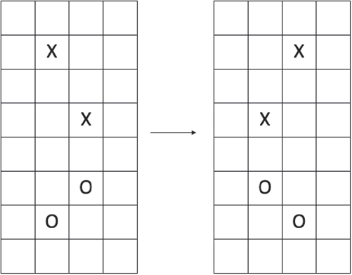
We begin with a brief summary of grid homology, a knot invariant first defined in [Reference Manolescu, Ozsváth and Sarkar2]. For this section, fix an oriented link $L\subset S^3$
. (For the majority of the paper, we will not worry too much about orientations as the grid homology of an oriented knot and that of its reverse are isomorphic.) A grid diagram is an n-by-n grid of squares such that there is one X and one O in each row and each column. We may retrieve a link from a grid diagram as follows. For each row and each column of squares, draw a line segment connecting the X to the O within that row or column, respectively. We assign each segment an orientation by specifying that vertical line segments point from X to O while horizontal line segments point from O to
$L\subset S^3$
. (For the majority of the paper, we will not worry too much about orientations as the grid homology of an oriented knot and that of its reverse are isomorphic.) A grid diagram is an n-by-n grid of squares such that there is one X and one O in each row and each column. We may retrieve a link from a grid diagram as follows. For each row and each column of squares, draw a line segment connecting the X to the O within that row or column, respectively. We assign each segment an orientation by specifying that vertical line segments point from X to O while horizontal line segments point from O to $X.$
Specify further that whenever two such segments intersect, the vertical segment crosses over the horizontal segments. Then, it is clear that the union of all these segments is an oriented planar link diagram. There exists a grid diagram representing any oriented link, in particular
$X.$
Specify further that whenever two such segments intersect, the vertical segment crosses over the horizontal segments. Then, it is clear that the union of all these segments is an oriented planar link diagram. There exists a grid diagram representing any oriented link, in particular $L,$
as guaranteed by [Reference Ozsváth, Stipcisz and Szabó5, Theorem 3.1.3]. Let
$L,$
as guaranteed by [Reference Ozsváth, Stipcisz and Szabó5, Theorem 3.1.3]. Let $\mathbb {G}$
be such a diagram.
$\mathbb {G}$
be such a diagram.
Denote by $\mathbb {X}$
the set of all the center points of the X-marked squares, and likewise denote by
$\mathbb {X}$
the set of all the center points of the X-marked squares, and likewise denote by $\mathbb {O}$
the set of all the center points of the O-marked squares. We consider
$\mathbb {O}$
the set of all the center points of the O-marked squares. We consider $\mathbb {G}$
to be a fundamental domain of a torus
$\mathbb {G}$
to be a fundamental domain of a torus $\mathbb {T}$
constructed by gluing opposite sides of
$\mathbb {T}$
constructed by gluing opposite sides of $\mathbb {G}.$
It is clear that different fundamental domains of this torus represent isotopic links. Fix a coordinate system on a fundamental domain corresponding to the cardinal directions North, South, East, and West.
$\mathbb {G}.$
It is clear that different fundamental domains of this torus represent isotopic links. Fix a coordinate system on a fundamental domain corresponding to the cardinal directions North, South, East, and West.
Call the horizontal circles formed by the edges of the grid of squares as $\alpha _1, \dots , \alpha _n,$
moving further north, and the vertical circles formed by the edges of the grid of squares as
$\alpha _1, \dots , \alpha _n,$
moving further north, and the vertical circles formed by the edges of the grid of squares as $\beta _1, \dots , \beta _n,$
moving further east. Let
$\beta _1, \dots , \beta _n,$
moving further east. Let $\boldsymbol \alpha $
denote
$\boldsymbol \alpha $
denote $\alpha _1\cup \dots \cup \alpha _n$
and
$\alpha _1\cup \dots \cup \alpha _n$
and $\boldsymbol \beta $
denote
$\boldsymbol \beta $
denote $\beta _1\cup \dots \cup \beta _n$
.
$\beta _1\cup \dots \cup \beta _n$
.
Definition 2.1 A grid state $\mathbf {x}$
of
$\mathbf {x}$
of $\mathbb {G}$
is a set of n points on
$\mathbb {G}$
is a set of n points on $\mathbb {T}$
such that
$\mathbb {T}$
such that $\lvert \mathbf {x}\cap \alpha _i\rvert =1$
for all
$\lvert \mathbf {x}\cap \alpha _i\rvert =1$
for all $i\in \{1,\dots , n\}$
and
$i\in \{1,\dots , n\}$
and $\lvert \mathbf {x}\cap \beta _i\rvert =1$
for all
$\lvert \mathbf {x}\cap \beta _i\rvert =1$
for all $i\in \{1,\dots , n\}.$
(In other words,
$i\in \{1,\dots , n\}.$
(In other words, $\mathbf {x}$
is a set of n intersection points of the
$\mathbf {x}$
is a set of n intersection points of the $\alpha $
and
$\alpha $
and $\beta $
curves, such that each curve is represented once.)
$\beta $
curves, such that each curve is represented once.)
We denote the set of all grid states of $\mathbb {G}$
by
$\mathbb {G}$
by $\mathbf {S}(\mathbb {G}).$
If $\mathbf {x}$
and
$\mathbf {x}$
and $\mathbf {y}$
are two grid states of a grid diagram
$\mathbf {y}$
are two grid states of a grid diagram $\mathbb {G},$
then we let the difference
$\mathbb {G},$
then we let the difference $\mathbf {x} - \mathbf {y}$
denote the oriented 0-manifold whose positive points are the points of
$\mathbf {x} - \mathbf {y}$
denote the oriented 0-manifold whose positive points are the points of $\mathbf {x} - \mathbf {x}\cap \mathbf {y}$
and whose negative points are the points of
$\mathbf {x} - \mathbf {x}\cap \mathbf {y}$
and whose negative points are the points of $\mathbf {y} - \mathbf {x}\cap \mathbf {y}.$
Definition 2.2 A rectangle r in $\mathbb {G}$
is an embedding of the closed unit disk
$\mathbb {G}$
is an embedding of the closed unit disk $D^2$
into
$D^2$
into $\mathbb {G}$
with four sides such that
$\mathbb {G}$
with four sides such that $\partial D^2$
gets mapped into the union of the
$\partial D^2$
gets mapped into the union of the $\alpha $
and
$\alpha $
and $\beta $
curves. Let
$\beta $
curves. Let
 $$ \begin{align*} A := \partial r\cap\boldsymbol\alpha. \end{align*} $$
Then A is a 1-manifold with boundary consisting of two line segments, and has an orientation induced from r by moving counterclockwise around the boundary $\partial r.$
We say the rectangle r connects two grid states
$\partial r.$
We say the rectangle r connects two grid states $\mathbf {x},\mathbf {y}\in \mathbf {S}(\mathbb {G})$
(or goes from
$\mathbf {x},\mathbf {y}\in \mathbf {S}(\mathbb {G})$
(or goes from $\mathbf {x}$
to
$\mathbf {x}$
to $\mathbf {y}$
) if
$\mathbf {y}$
) if $\partial A = \mathbf {y} - \mathbf {x}$
as oriented 0-manifolds.
$\partial A = \mathbf {y} - \mathbf {x}$
as oriented 0-manifolds.
The set of all rectangles from $\mathbf {x}$
to
$\mathbf {x}$
to $\mathbf {y}$
is denoted by
$\mathbf {y}$
is denoted by $\operatorname {\mathrm {Rect}}(\mathbf {x}, \mathbf {y}).$
We wish to create two functions M and A from $\mathbf {S}(\mathbb {G})$
to
$\mathbf {S}(\mathbb {G})$
to $\mathbb {Z},$
which we define as follows.
$\mathbb {Z},$
which we define as follows.
Definition 2.3 Let P and Q be finite sets of points in a fundamental domain for $\mathbb {G},$
which we may embed in
$\mathbb {G},$
which we may embed in $\mathbb {R}^2$
with standard Cartesian coordinates as the rectangle
$\mathbb {R}^2$
with standard Cartesian coordinates as the rectangle $[0, n)\times [0, n)$
such that each square in
$[0, n)\times [0, n)$
such that each square in $\mathbb {G}$
is a unit square with integral coordinates for its corners. Let
$\mathbb {G}$
is a unit square with integral coordinates for its corners. Let $\ell $
be the number of components of the link described by
$\ell $
be the number of components of the link described by $\mathbb {G}.$
Then, we define
$\mathbb {G}.$
Then, we define $\mathcal {I}(P, Q)$
to be the number of pairs of points
$\mathcal {I}(P, Q)$
to be the number of pairs of points $(p_1, p_2)\times (q_1, q_2)\in P\times Q$
satisfying
$(p_1, p_2)\times (q_1, q_2)\in P\times Q$
satisfying $p_1<q_1$
and
$p_1<q_1$
and $p_2<q_2.$
Now, let
$p_2<q_2.$
Now, let
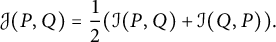 $$ \begin{align*}\mathcal{J}(P, Q) = \frac12(\mathcal{I}(P, Q) + \mathcal{I}(Q, P)).\end{align*} $$
Then, we let
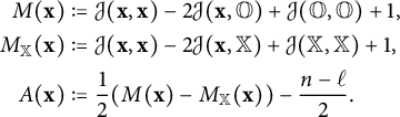 $$ \begin{align*} M(\mathbf{x}) &:= \mathcal{J}(\mathbf{x}, \mathbf{x}) - 2\mathcal{J}(\mathbf{x}, \mathbb{O}) + \mathcal{J}(\mathbb{O}, \mathbb{O}) + 1, \nonumber \\ M_{\mathbb{X}}(\mathbf{x}) &:= \mathcal{J}(\mathbf{x}, \mathbf{x}) - 2\mathcal{J}(\mathbf{x}, \mathbb{X}) + \mathcal{J}(\mathbb{X}, \mathbb{X}) + 1, \nonumber \\ A(\mathbf{x}) &:= \frac12(M(\mathbf{x}) - M_{\mathbb{X}}(\mathbf{x})) - \frac{n-\ell}{2}. \nonumber \end{align*} $$
We call $M(\mathbf {x})$
the Maslov grading and
$M(\mathbf {x})$
the Maslov grading and $A(\mathbf {x})$
the Alexander grading, and we call the pair
$A(\mathbf {x})$
the Alexander grading, and we call the pair $(M, A)$
the bigrading of
$(M, A)$
the bigrading of $\mathbf {x}.$
The below proposition is greatly helpful to our future ventures.
Proposition 2.4
-
• Both M and A are integral-valued functions (note it is only clear from their definitions that they are half-integral valued).
Suppose $\mathbf {x}$
and
$\mathbf {x}$
and $\mathbf {y}$
are two grid states with some rectangle
$\mathbf {y}$
are two grid states with some rectangle $r\in \operatorname {\mathrm {Rect}}(\mathbf {x}, \mathbf {y}).$
Then, their Maslov and Alexander gradings are related by the following formulas:
$r\in \operatorname {\mathrm {Rect}}(\mathbf {x}, \mathbf {y}).$
Then, their Maslov and Alexander gradings are related by the following formulas:
-
• $M(\mathbf {x}) - M(\mathbf {y}) = 1 - 2\lvert r\cap \mathbb {O}\rvert + 2\lvert \mathbf {x}\cap \operatorname {\mathrm {Int}}(r)\lvert .$
-
•
$A(\mathbf {x}) - A(\mathbf {y}) = \lvert r\cap \mathbb {X}\rvert - \lvert r\cap \mathbb {O}\rvert .$


The proof is found in [Reference Ozsváth, Stipcisz and Szabó5, Section 4.3], and is elementary but rather long.
Definition 2.5 Let a domain $\psi $
in
$\psi $
in $\mathbb {G}$
be any formal
$\mathbb {G}$
be any formal $\mathbb {Z}$
-linear combination of squares in
$\mathbb {Z}$
-linear combination of squares in $\mathbb {G}$
(which may be defined as the closures of the connected components of
$\mathbb {G}$
(which may be defined as the closures of the connected components of $\mathbb {T}-\boldsymbol \alpha \cup \boldsymbol \beta $
).
$\mathbb {T}-\boldsymbol \alpha \cup \boldsymbol \beta $
).
Again, the boundary of a domain inherits a counterclockwise orientation. We say a domain connects two grid states $\mathbf {x}$
and
$\mathbf {x}$
and $\mathbf {z}$
in
$\mathbf {z}$
in $\mathbf {S}(\mathbb {G})$
if
$\mathbf {S}(\mathbb {G})$
if
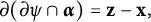 $$ \begin{align*}\partial(\partial \psi\cap\boldsymbol\alpha) = \mathbf{z} - \mathbf{x},\end{align*} $$
as oriented 0-manifolds. Let the set of all domains from $\mathbf {x}$
to
$\mathbf {x}$
to $\mathbf {z}$
be denoted as
$\mathbf {z}$
be denoted as $\pi (\mathbf {x}, \mathbf {z}).$
For a domain $\psi $
and a point
$\psi $
and a point $p\in \mathbb {T}-\boldsymbol \alpha \cup \boldsymbol \beta $
, let
$p\in \mathbb {T}-\boldsymbol \alpha \cup \boldsymbol \beta $
, let $\psi (p)$
be the multiplicity of
$\psi (p)$
be the multiplicity of $\psi $
at the point
$\psi $
at the point $p.$
$p.$
We say a domain $\psi \in \pi (\mathbf {x}, \mathbf {z})$
can be decomposed as a juxtaposition of two rectangles
$\psi \in \pi (\mathbf {x}, \mathbf {z})$
can be decomposed as a juxtaposition of two rectangles $r_1\in \operatorname {\mathrm {Rect}}(\mathbf {x}, \mathbf {y})$
and
$r_1\in \operatorname {\mathrm {Rect}}(\mathbf {x}, \mathbf {y})$
and $r_2\in \operatorname {\mathrm {Rect}}(\mathbf {y}, \mathbf {z})$
, and write
$r_2\in \operatorname {\mathrm {Rect}}(\mathbf {y}, \mathbf {z})$
, and write $\psi = r_1*r_2$
, if
$\psi = r_1*r_2$
, if $\psi = r_1+r_2$
as linear combinations of squares.
$\psi = r_1+r_2$
as linear combinations of squares.
We are now ready to define grid homology. For the remainder of this paper, let $\mathbb {F}$
represent the field of two elements
$\mathbb {F}$
represent the field of two elements $\mathbb {Z}/2\mathbb {Z}.$
Definition 2.6 Let $\mathbb {G}$
be a grid diagram. We define the chain complex
$\mathbb {G}$
be a grid diagram. We define the chain complex $\mathit {GC}^-(\mathbb {G})$
to be the free
$\mathit {GC}^-(\mathbb {G})$
to be the free $\mathbb {F}[V_1,\dots , V_n]$
-module generated by the grid states of
$\mathbb {F}[V_1,\dots , V_n]$
-module generated by the grid states of $\mathbb {G},$
with
$\mathbb {G},$
with $V_1^{k_1}\dots V_n^{k_n}\mathbf {x}$
having bigrading
$V_1^{k_1}\dots V_n^{k_n}\mathbf {x}$
having bigrading
 $$ \begin{align*}(M(\mathbf{x})-2k_1-\dots-2k_n, A(\mathbf{x})-k_1-\dots-k_n).\end{align*} $$
Let $\partial _0:\mathit {GC}^-(\mathbb {G})\rightarrow \mathit {GC}^-(\mathbb {G})$
be given as
$\partial _0:\mathit {GC}^-(\mathbb {G})\rightarrow \mathit {GC}^-(\mathbb {G})$
be given as
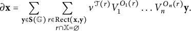
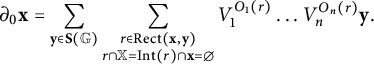 $$ \begin{align*}\partial_0\mathbf{x} = \sum_{\mathbf{y}\in\mathbf{S}(\mathbb{G})}\sum_{\substack{ r\in\operatorname{\mathrm{Rect}}(\mathbf{x}, \mathbf{y}) \\ r\cap\mathbb{X} = \operatorname{\mathrm{Int}}(r)\cap\mathbf{x}=\emptyset \\}} V_1^{O_1(r)}\dots V_n^{O_n(r)}\mathbf{y}.\end{align*} $$
[Reference Ozsváth, Stipcisz and Szabó5, Chapter 4] demonstrates that $\partial _0$
is a homogeneous map of bidegree
$\partial _0$
is a homogeneous map of bidegree $(-1, 0)$
and
$(-1, 0)$
and $\partial _0^2=0,$
hence
$\partial _0^2=0,$
hence $\partial _0$
is a differential on
$\partial _0$
is a differential on $\mathit {GC}^-(\mathbb {G})$
and the homology of the chain complex
$\mathit {GC}^-(\mathbb {G})$
and the homology of the chain complex $(\mathit {GC}^-(\mathbb {G}), \partial _0)$
is well-defined. We denote this homology as
$(\mathit {GC}^-(\mathbb {G}), \partial _0)$
is well-defined. We denote this homology as $\mathit {GH}^-(\mathbb {G}).$
[Reference Ozsváth, Stipcisz and Szabó5, Chapter 5] proves that the action of each $V_i$
is identical on the level of homology. Calling this action by
$V_i$
is identical on the level of homology. Calling this action by $U,$
that the bigraded
$U,$
that the bigraded $\mathbb {F}[U]$
-module isomorphism type of
$\mathbb {F}[U]$
-module isomorphism type of $\mathit {GH}^-(\mathbb {G})$
is an invariant of the (unoriented) knot K; we may write it as
$\mathit {GH}^-(\mathbb {G})$
is an invariant of the (unoriented) knot K; we may write it as $\mathit {GH}^-(K).$
We also may create a variant of this construction that gives us a bigraded $\mathbb {F}$
-vector space. For a knot, consider the quotient complex
$\mathbb {F}$
-vector space. For a knot, consider the quotient complex $\mathit {GC}^-(\mathbb {G})/(V_n = 0)$
as a vector space over
$\mathit {GC}^-(\mathbb {G})/(V_n = 0)$
as a vector space over $\mathbb {F},$
and let the differential
$\mathbb {F},$
and let the differential $\widehat {\partial _0}$
on this complex be induced from
$\widehat {\partial _0}$
on this complex be induced from $\partial _0.$
For a link of
$\partial _0.$
For a link of $\ell $
components, first label the components from 1 to
$\ell $
components, first label the components from 1 to $\ell .$
On the ith component, choose an O-marking
$\ell .$
On the ith component, choose an O-marking $O_{n_i}$
on that component. Now, consider the quotient complex
$O_{n_i}$
on that component. Now, consider the quotient complex $\mathit {GC}^-(\mathbb {G})/(V_{n_i} = 0 ~\text {for all }i)$
as a vector space over
$\mathit {GC}^-(\mathbb {G})/(V_{n_i} = 0 ~\text {for all }i)$
as a vector space over $\mathbb {F},$
and let the differential
$\mathbb {F},$
and let the differential $\widehat {\partial _0}$
on this complex be induced from
$\widehat {\partial _0}$
on this complex be induced from $\partial _0.$
Definition 2.7 The homology of the complex $(\mathit {GC}^-(\mathbb {G})/(V_n = 0), \widehat {\partial _0}),$
(or the more general version for links) as a bigraded
$(\mathit {GC}^-(\mathbb {G})/(V_n = 0), \widehat {\partial _0}),$
(or the more general version for links) as a bigraded $\mathbb {F}$
-vector space, is referred to as
$\mathbb {F}$
-vector space, is referred to as $\widehat {\mathit {GH}}(\mathbb {G}).$
[Reference Ozsváth, Stipcisz and Szabó5, Chapter 5] proves that the bigraded $\mathbb {F}$
-vector space isomorphism type of
$\mathbb {F}$
-vector space isomorphism type of $\mathit {GH}^-(\mathbb {G})$
is also an invariant of the knot K, and a similar argument shows this remains true for links.
$\mathit {GH}^-(\mathbb {G})$
is also an invariant of the knot K, and a similar argument shows this remains true for links.
2.1 Grid moves
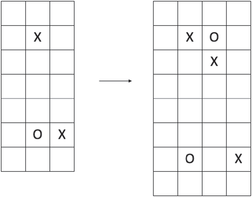
We would like a way to relate any two grid representations of the same (oriented) link. We define three types of grid moves: commutations, switches, and stabilizations.
Definition 2.8 Consider two adjacent rows (resp., columns) of a grid diagram in a fundamental domain, and draw the (closed) line segments joining the X- and O- markings in each row (resp., column). Project these two line segments onto the horizontal (resp., vertical) axis. If either (1) the two projected line segments have disjoint supports or (2) one of the projected line segments lies in the interior of the other, then swapping the two adjacent rows (resp., columns) is called a commutation.
If the two projected line segments share a vertex, then swapping the two adjacent rows (resp., columns) is called a switch.
Here, we picture a commutation:
Definition 2.9 Consider a square marked with an X (resp., an O). Choose one of the following four directions, $NE, NW, SE, SW.$
Subdivide the row and column containing the X (resp., O) so that
$NE, NW, SE, SW.$
Subdivide the row and column containing the X (resp., O) so that $\mathbb {G}$
is now an
$\mathbb {G}$
is now an $n+1$
-by-
$n+1$
-by- $n+1$
grid diagram, and the square formerly containing the X (resp., O) is now a 2-by-2 grid. Replace the X (resp., O) with two X’s in the diagonal of this 2-by-2 grid that does not contain the chosen direction, and an O (resp., X) in a third square of this 2-by-2 grid such that the unmarked square is the one corresponding to the chosen direction. This operation is known as a stabilization of type X:direction (resp., O:direction). Its inverse is known as a destabilization of the corresponding type.
$n+1$
grid diagram, and the square formerly containing the X (resp., O) is now a 2-by-2 grid. Replace the X (resp., O) with two X’s in the diagonal of this 2-by-2 grid that does not contain the chosen direction, and an O (resp., X) in a third square of this 2-by-2 grid such that the unmarked square is the one corresponding to the chosen direction. This operation is known as a stabilization of type X:direction (resp., O:direction). Its inverse is known as a destabilization of the corresponding type.
Here, we picture a stabilization of type X: $SW$
:
$SW$
:
The following theorem, which comes from [Reference Ozsváth, Stipcisz and Szabó5, Corollary 3.2.3], will prove extremely useful in showing invariance of double-point enhanced grid homology.
Theorem 2.10 (Generalized from Cromwell)
Any two grid diagrams of the same (oriented) knot are related by a finite sequence of commutations, switches, and stabilizations and destabilizations of the form X: $SW$
.
$SW$
.
3 Double-point enhanced grid homology notation
Definition 3.1 Fix an n-by-n grid diagram $\mathbb {G}$
. We define a bigraded chain complex of free
$\mathbb {G}$
. We define a bigraded chain complex of free $\mathbb {F}[V_1,\dots , V_n, v]$
-modules
$\mathbb {F}[V_1,\dots , V_n, v]$
-modules $\mathit {GCL}^-(\mathbb {G})$
as follows. As a bigraded module,
$\mathit {GCL}^-(\mathbb {G})$
as follows. As a bigraded module, $\mathit {GCL}^-(\mathbb {G}) = \mathit {GC}^-(\mathbb {G})[v]$
, where if
$\mathit {GCL}^-(\mathbb {G}) = \mathit {GC}^-(\mathbb {G})[v]$
, where if $\xi \in \mathit {GC}^-(\mathbb {G})$
is homogeneous of bidegree
$\xi \in \mathit {GC}^-(\mathbb {G})$
is homogeneous of bidegree $(M, A),$
then
$(M, A),$
then $v^k\xi $
is homogeneous of bidegree
$v^k\xi $
is homogeneous of bidegree $(M+2k, A).$
We define a differential
 $$ \begin{align*}\partial\xi := \sum_{k=0}^{\infty} v^k\partial_k\xi,\end{align*} $$
where $\partial _k$
is defined on grid states by
$\partial _k$
is defined on grid states by
 $$ \begin{align*}\partial_k\mathbf{x}= \sum_{\mathbf{y}\in\mathbf{S}(\mathbb{G})}\sum_{\substack{r\in\operatorname{\mathrm{Rect}}(\mathbf{x}, \mathbf{y}) \\ r\cap\mathbb{X} = \emptyset \\ \lvert\operatorname{\mathrm{Int}}(r)\cap\mathbf{x}\rvert = k \\}} V_1^{O_1(r)}\dots V_n^{O_n(r)}\mathbf{y}, \end{align*} $$
and extends by linearity.
Proposition 3.2 The map $\partial $
is indeed a differential, that is,
$\partial $
is indeed a differential, that is, $\partial ^2=0.$
We shall prove a more general version of this proposition later, see 5.5. For now, we take this for granted, and let $\mathit {GHL}^-(\mathbb {G})$
denote the homology of the chain complex
$\mathit {GHL}^-(\mathbb {G})$
denote the homology of the chain complex $(\mathit {GCL}^-(\mathbb {G}), \partial ).$
We will need to generalize some constructions in the proof of invariance of $\mathit {GH}^-$
found in [Reference Ozsváth, Stipcisz and Szabó5] in order to prove analogous results in the double-point enhanced case. The issue arises as follows. To show
$\mathit {GH}^-$
found in [Reference Ozsváth, Stipcisz and Szabó5] in order to prove analogous results in the double-point enhanced case. The issue arises as follows. To show $\partial _0^2 = 0$
in the un-enhanced case, we start with a grid state
$\partial _0^2 = 0$
in the un-enhanced case, we start with a grid state $\mathbf {x}\in \mathbf {S}(\mathbb {G}).$
Next, we compute that if
$\mathbf {x}\in \mathbf {S}(\mathbb {G}).$
Next, we compute that if $\mathbf {z}\in \mathbf {S}(\mathbb {G})$
is another grid state with
$\mathbf {z}\in \mathbf {S}(\mathbb {G})$
is another grid state with $\lvert \mathbf {x} - \mathbf {x}\cap \mathbf {z}\rvert = 3,$
then the
$\lvert \mathbf {x} - \mathbf {x}\cap \mathbf {z}\rvert = 3,$
then the $\mathbf {z}$
-coefficient of
$\mathbf {z}$
-coefficient of $\partial _0^2(\mathbf {x})$
counts the number of decompositions into two rectangles of L-shaped domains connecting
$\partial _0^2(\mathbf {x})$
counts the number of decompositions into two rectangles of L-shaped domains connecting $\mathbf {x}$
to
$\mathbf {x}$
to $\mathbf {z}.$
Finally, we show that each such domain has an even number of decompositions. This line of argument works because every L-shaped domain of two empty rectangles, that is rectangles
$\mathbf {z}.$
Finally, we show that each such domain has an even number of decompositions. This line of argument works because every L-shaped domain of two empty rectangles, that is rectangles $r\in \operatorname {\mathrm {Rect}}(\mathbf {x}, \mathbf {y})$
with
$r\in \operatorname {\mathrm {Rect}}(\mathbf {x}, \mathbf {y})$
with $\operatorname {\mathrm {Int}}(r)\cap \mathbf {x} = \emptyset ,$
has exactly two decompositions in terms of empty rectangles. We use this similar line of argument to prove that the actions of multiplying by each
$\operatorname {\mathrm {Int}}(r)\cap \mathbf {x} = \emptyset ,$
has exactly two decompositions in terms of empty rectangles. We use this similar line of argument to prove that the actions of multiplying by each $V_i$
are all chain-homotopic to each other, to show the invariance of
$V_i$
are all chain-homotopic to each other, to show the invariance of $\mathit {GH}^-$
under commutation moves, and also to show vital lemmas in the proof of the skein relation.
$\mathit {GH}^-$
under commutation moves, and also to show vital lemmas in the proof of the skein relation.
While the proof that $\partial _0^2 = 0$
proceeds as we would hope when the rectangles are no longer required to be empty, many of the other proofs mentioned above break down. Specifically, L-shaped domains of not-necessarily-empty rectangles do not necessarily admit exactly two decompositions. For a counter-example, see [Reference Ratigan, Wang and Wang9, Section 2.2]. In order to treat this difficulty, I present a few definitions below of a new concept known as “long rectangles,” which will recur throughout the paper. The essential idea is that we introduce a larger class of rectangles such that every L-shaped decomposition still has two decompositions into these generalized rectangles.
$\partial _0^2 = 0$
proceeds as we would hope when the rectangles are no longer required to be empty, many of the other proofs mentioned above break down. Specifically, L-shaped domains of not-necessarily-empty rectangles do not necessarily admit exactly two decompositions. For a counter-example, see [Reference Ratigan, Wang and Wang9, Section 2.2]. In order to treat this difficulty, I present a few definitions below of a new concept known as “long rectangles,” which will recur throughout the paper. The essential idea is that we introduce a larger class of rectangles such that every L-shaped decomposition still has two decompositions into these generalized rectangles.
In contrast, the solution to this problem laid out in [Reference Ratigan, Wang and Wang9] is to use a four-fold cover of the torus and consider rectangles in this larger space (they call these four-fold toroidal grid diagrams.) My reformulation of this idea using “long rectangles,” a bit more convenient for some of the applications later in the paper, but mathematically it is equivalent to the treatment in [Reference Ratigan, Wang and Wang9]. Specifically, we will be able to define long polygons in analogy with long rectangles, and when we discuss extending the coefficients over $\mathbb {Z},$
we will be able to assign signs to long polygons.
$\mathbb {Z},$
we will be able to assign signs to long polygons.
For any toroidal grid diagram on a torus $\mathbb {T}$
, we may consider the universal cover of the torus, which we identify with
$\mathbb {T}$
, we may consider the universal cover of the torus, which we identify with $\mathbb {R}^2$
and its standard
$\mathbb {R}^2$
and its standard $(x,y)$
Cartesian coordinates. Here, lifts of the
$(x,y)$
Cartesian coordinates. Here, lifts of the $\alpha _i$
and
$\alpha _i$
and $\beta _j$
curves, which we may call
$\beta _j$
curves, which we may call $\tilde {\alpha }_i$
,
$\tilde {\alpha }_i$
, $\tilde {\beta }_j$
, respectively, are the straight lines
$\tilde {\beta }_j$
, respectively, are the straight lines $y=n$
and
$y=n$
and $x=m$
as
$x=m$
as $n,m$
range over
$n,m$
range over $\mathbb {Z}.$
Definition 3.3 Consider a rectangle R of width 1 or height 1 in $\mathbb {R}^2$
whose sides lie along the
$\mathbb {R}^2$
whose sides lie along the $\tilde {\alpha }_i$
,
$\tilde {\alpha }_i$
, $\tilde {\beta }_j$
lines, and such that the projection of R onto
$\tilde {\beta }_j$
lines, and such that the projection of R onto $\mathbb {T}$
, which we call r, has multiplicity
$\mathbb {T}$
, which we call r, has multiplicity $2$
in at least one point, and multiplicity 1 in at least one point. Then, we call r a long rectangle.
$2$
in at least one point, and multiplicity 1 in at least one point. Then, we call r a long rectangle.
Note that r is a domain in $\mathbb {G},$
and it connects grid states analogously to ordinary rectangles. We denote by
$\mathbb {G},$
and it connects grid states analogously to ordinary rectangles. We denote by $\operatorname {\mathrm {Rect}}^{*}(\mathbf {x}, \mathbf {y})$
the set of rectangles and long rectangles from grid state
$\operatorname {\mathrm {Rect}}^{*}(\mathbf {x}, \mathbf {y})$
the set of rectangles and long rectangles from grid state $\mathbf {x}\in \mathbf {S}(\mathbb {G})$
to
$\mathbf {x}\in \mathbf {S}(\mathbb {G})$
to $\mathbf {y}\in \mathbf {S}(\mathbb {G}).$
Remark 3.4 Unlike the treatment in [Reference Ratigan, Wang and Wang9], we only need to introduce long rectangles of width 1 or height 1.
Definition 3.5 We define the function $\mathcal {T}:\operatorname {\mathrm {Rect}}^{*}(\mathbf {x}, \mathbf {y})\rightarrow \mathbb {Z}_{\geq 0}$
as follows. Let
$\mathcal {T}:\operatorname {\mathrm {Rect}}^{*}(\mathbf {x}, \mathbf {y})\rightarrow \mathbb {Z}_{\geq 0}$
as follows. Let $r\in \operatorname {\mathrm {Rect}}^{*}(\mathbf {x}, \mathbf {y}).$
If r is long, then
$r\in \operatorname {\mathrm {Rect}}^{*}(\mathbf {x}, \mathbf {y}).$
If r is long, then $\mathcal {T}(r)=1,$
and if r is not long, then
$\mathcal {T}(r)=1,$
and if r is not long, then $\mathcal {T}(r) = \lvert \operatorname {\mathrm {Int}}(r)\cap \mathbf {x}\rvert .$
Remark 3.6 Note that we can now rewrite the differential $\partial $
more compactly as
$\partial $
more compactly as
 $$ \begin{align*}\partial\mathbf{x}= \sum_{\mathbf{y}\in\mathbf{S}(\mathbb{G})}\sum_{\substack{r\in\operatorname{\mathrm{Rect}}(\mathbf{x}, \mathbf{y}) \\ r\cap\mathbb{X} = \emptyset\\ }} v^{\mathcal{T}(r)}V_1^{O_1(r)}\dots V_n^{O_n(r)}\mathbf{y}.\end{align*} $$
Definition 3.7 Let $\mathbf {x}, \mathbf {z}\in \mathbf {S}(\mathbb {G}),$
and suppose
$\mathbf {x}, \mathbf {z}\in \mathbf {S}(\mathbb {G}),$
and suppose $\psi \in \pi (\mathbf {x}, \mathbf {z})$
is a domain, with decomposition
$\psi \in \pi (\mathbf {x}, \mathbf {z})$
is a domain, with decomposition $\psi = r_1*r_2$
for
$\psi = r_1*r_2$
for $r_1\in \operatorname {\mathrm {Rect}}^{*}(\mathbf {x},\mathbf {y})$
and
$r_1\in \operatorname {\mathrm {Rect}}^{*}(\mathbf {x},\mathbf {y})$
and $r_2\in \operatorname {\mathrm {Rect}}^{*}(\mathbf {y},\mathbf {z}).$
The degree of the decomposition, which we will notate as
$r_2\in \operatorname {\mathrm {Rect}}^{*}(\mathbf {y},\mathbf {z}).$
The degree of the decomposition, which we will notate as $\deg (r_1, r_2),$
is defined as the sum:
$\deg (r_1, r_2),$
is defined as the sum:
 $$ \begin{align*}\deg(r_1, r_2) = \mathcal{T}(r_1)+\mathcal{T}(r_2).\end{align*} $$
Definition 3.8 For a rectangle or long rectangle $r\in \operatorname {\mathrm {Rect}}^{*}(\mathbf {x}, \mathbf {y})$
, the incoming corners are precisely the members of
$r\in \operatorname {\mathrm {Rect}}^{*}(\mathbf {x}, \mathbf {y})$
, the incoming corners are precisely the members of $\partial r\cap \mathbf {x},$
and the outgoing corners are precisely the members of
$\partial r\cap \mathbf {x},$
and the outgoing corners are precisely the members of $\partial r\cap \mathbf {y}.$
3.1 For commutation/switch invariance
To prove invariance of grid homology under commutation and switch moves, and also to prove the skein exact sequence, we will require superimposing two grid diagrams $\mathbb {G}$
and
$\mathbb {G}$
and $\mathbb {G}'$
differing by a commutation or switch as pictured in the below picture of the relevant portion of this superimposed diagram:
$\mathbb {G}'$
differing by a commutation or switch as pictured in the below picture of the relevant portion of this superimposed diagram:
We call $\beta _i$
the curved circle belonging to
$\beta _i$
the curved circle belonging to $\mathbb {G}$
and
$\mathbb {G}$
and $\gamma _i$
the curved circle belonging to
$\gamma _i$
the curved circle belonging to $\mathbb {G}'.$
Let a and b be the two intersections of
$\mathbb {G}'.$
Let a and b be the two intersections of $\beta _i$
and
$\beta _i$
and $\gamma _i,$
with a at the southern end of the bigon containing
$\gamma _i,$
with a at the southern end of the bigon containing $\beta _i$
as its western boundary.
$\beta _i$
as its western boundary.
Remark 3.9 Very importantly, we may always assume that each bigon contains at least one X-marking in it. We will be counting regions that are forbidden from intersecting X-markings, hence this assumption will markedly simplify our below analysis.
Definition 3.10 (Modified from [Reference Ozsváth, Stipcisz and Szabó5, Definition 5.1.1])
A pentagon from $\mathbf {x}\in \mathbf {S}(\mathbb {G})$
to
$\mathbf {x}\in \mathbf {S}(\mathbb {G})$
to $\mathbf {y}'\in \mathbf {S}(\mathbb {G}')$
is an embedded disk p in the torus whose boundary is the union of five arcs, each of which lies on an
$\mathbf {y}'\in \mathbf {S}(\mathbb {G}')$
is an embedded disk p in the torus whose boundary is the union of five arcs, each of which lies on an $\alpha _j, \beta _j,$
or
$\alpha _j, \beta _j,$
or $\gamma _i$
curve, such that: (1) four of the corners of p are in
$\gamma _i$
curve, such that: (1) four of the corners of p are in $\mathbf {x}\cup \mathbf {y}',$
(2) at each corner x of
$\mathbf {x}\cup \mathbf {y}',$
(2) at each corner x of $p,$
exactly one of the four quadrants of a small disk surrounding x has multiplicity 1 and the other three have multiplicity 0, and (3)
$p,$
exactly one of the four quadrants of a small disk surrounding x has multiplicity 1 and the other three have multiplicity 0, and (3)
 $$ \begin{align*}\partial(\partial p\cap\boldsymbol\alpha) = \mathbf{y}' - \mathbf{x}.\end{align*} $$
Let P be an embedded disk in the universal cover of the torus satisfying conditions (1)–(3), satisfying two extra conditions: (4) that P has width one, and (5), that the projection of P onto the torus, which we call p, has multiplicity $2$
in at least one point, and multiplicity 1 in at least one point. Then, we call p a long pentagon from
$2$
in at least one point, and multiplicity 1 in at least one point. Then, we call p a long pentagon from $\mathbf {x}$
to
$\mathbf {x}$
to $\mathbf {y}'.$
Let $\operatorname {\mathrm {Pent}}(\mathbf {x}, \mathbf {y}')$
denote the set of pentagons from
$\operatorname {\mathrm {Pent}}(\mathbf {x}, \mathbf {y}')$
denote the set of pentagons from $\mathbf {x}$
to
$\mathbf {x}$
to $\mathbf {y}',$
and
$\mathbf {y}',$
and $\operatorname {\mathrm {Pent}}^{*}(\mathbf {x}, \mathbf {y}')$
denote the set of pentagons and long pentagons from
$\operatorname {\mathrm {Pent}}^{*}(\mathbf {x}, \mathbf {y}')$
denote the set of pentagons and long pentagons from $\mathbf {x}$
to
$\mathbf {x}$
to $\mathbf {y}'.$
Definition 3.11 (Modified from [Reference Ozsváth, Stipcisz and Szabó5, Definition 5.1.5])
A hexagon from $\mathbf {x}\in \mathbf {S}(\mathbb {G})$
to
$\mathbf {x}\in \mathbf {S}(\mathbb {G})$
to $\mathbf {y}\in \mathbf {S}(\mathbb {G})$
is an embedded disk h in the torus whose boundary is the union of six arcs, each of which lies on an
$\mathbf {y}\in \mathbf {S}(\mathbb {G})$
is an embedded disk h in the torus whose boundary is the union of six arcs, each of which lies on an $\alpha _j, \beta _j,$
or
$\alpha _j, \beta _j,$
or $\gamma _i$
curve, such that: (1) four of the corners of h are in
$\gamma _i$
curve, such that: (1) four of the corners of h are in $\mathbf {x}\cup \mathbf {y}',$
and the other two corners are at a and b, (2) at each corner x of
$\mathbf {x}\cup \mathbf {y}',$
and the other two corners are at a and b, (2) at each corner x of $h,$
exactly one of the four quadrants of a small disk surrounding x has multiplicity 1 and the other three have multiplicity 0, and (3)
$h,$
exactly one of the four quadrants of a small disk surrounding x has multiplicity 1 and the other three have multiplicity 0, and (3)
 $$ \begin{align*}\partial(\partial h\cap\boldsymbol\alpha) = \mathbf{y} - \mathbf{x}.\end{align*} $$
Let H be an embedded disk in the universal cover of the torus satisfying conditions (1)–(3), satisfying two extra conditions: (4) that P has width one, and (5), that the projection of H onto the torus, which we call h, has multiplicity $2$
in at least one point, and multiplicity 1 in at least one point. Then, we call h a long pentagon from
$2$
in at least one point, and multiplicity 1 in at least one point. Then, we call h a long pentagon from $\mathbf {x}$
to
$\mathbf {x}$
to $\mathbf {y}.$
Let $\operatorname {\mathrm {Hex}}(\mathbf {x}, \mathbf {y})$
denote the set of pentagons from
$\operatorname {\mathrm {Hex}}(\mathbf {x}, \mathbf {y})$
denote the set of pentagons from $\mathbf {x}$
to
$\mathbf {x}$
to $\mathbf {y},$
and
$\mathbf {y},$
and $\operatorname {\mathrm {Hex}}^{*}(\mathbf {x}, \mathbf {y})$
denote the set of pentagons and long pentagons from
$\operatorname {\mathrm {Hex}}^{*}(\mathbf {x}, \mathbf {y})$
denote the set of pentagons and long pentagons from $\mathbf {x}$
to
$\mathbf {x}$
to $\mathbf {y}.$
Definition 3.12 We define the function $\mathcal {T}:\operatorname {\mathrm {Pent}}^{*}(\mathbf {x}, \mathbf {y}')\rightarrow \mathbb {Z}_{\geq 0}$
as follows. Let
$\mathcal {T}:\operatorname {\mathrm {Pent}}^{*}(\mathbf {x}, \mathbf {y}')\rightarrow \mathbb {Z}_{\geq 0}$
as follows. Let $p\in \operatorname {\mathrm {Pent}}^{*}(\mathbf {x}, \mathbf {y}).$
If p is long, then
$p\in \operatorname {\mathrm {Pent}}^{*}(\mathbf {x}, \mathbf {y}).$
If p is long, then $\mathcal {T}(p)=1,$
and if p is not long, then
$\mathcal {T}(p)=1,$
and if p is not long, then $\mathcal {T}(p) = \lvert \operatorname {\mathrm {Int}}(p)\cap \mathbf {x}\rvert .$
Similarly, we define the function
$\mathcal {T}(p) = \lvert \operatorname {\mathrm {Int}}(p)\cap \mathbf {x}\rvert .$
Similarly, we define the function $\mathcal {T}:\operatorname {\mathrm {Hex}}^{*}(\mathbf {x}, \mathbf {y}')\rightarrow \mathbb {Z}_{\geq 0}$
as follows. Let
$\mathcal {T}:\operatorname {\mathrm {Hex}}^{*}(\mathbf {x}, \mathbf {y}')\rightarrow \mathbb {Z}_{\geq 0}$
as follows. Let $h\in \operatorname {\mathrm {Hex}}^{*}(\mathbf {x}, \mathbf {y}).$
If h is long, then
$h\in \operatorname {\mathrm {Hex}}^{*}(\mathbf {x}, \mathbf {y}).$
If h is long, then $\mathcal {T}(h)=1,$
and if h is not long, then
$\mathcal {T}(h)=1,$
and if h is not long, then $\mathcal {T}(h) = \lvert \operatorname {\mathrm {Int}}(h)\cap \mathbf {x}\rvert .$
Definition 3.13 Let $\mathbf {x}, \mathbf {z}\in \mathbf {S}(\mathbb {G})\cup \mathbf {S}(\mathbb {G}'),$
and suppose
$\mathbf {x}, \mathbf {z}\in \mathbf {S}(\mathbb {G})\cup \mathbf {S}(\mathbb {G}'),$
and suppose $\psi \in \pi (\mathbf {x}, \mathbf {z})$
is a domain, with decomposition
$\psi \in \pi (\mathbf {x}, \mathbf {z})$
is a domain, with decomposition $\psi = r_1*r_2$
for
$\psi = r_1*r_2$
for $r_1\in \operatorname {\mathrm {Rect}}^{*}(\mathbf {x},\mathbf {y})\cup \operatorname {\mathrm {Pent}}^{*}(\mathbf {x},\mathbf {y})\cup \operatorname {\mathrm {Hex}}^{*}(\mathbf {x},\mathbf {y})$
and
$r_1\in \operatorname {\mathrm {Rect}}^{*}(\mathbf {x},\mathbf {y})\cup \operatorname {\mathrm {Pent}}^{*}(\mathbf {x},\mathbf {y})\cup \operatorname {\mathrm {Hex}}^{*}(\mathbf {x},\mathbf {y})$
and $r_2\in \operatorname {\mathrm {Rect}}^{*}(\mathbf {y},\mathbf {z})\cup \operatorname {\mathrm {Pent}}^{*}(\mathbf {y},\mathbf {z})\cup \operatorname {\mathrm {Hex}}^{*}(\mathbf {y},\mathbf {z}).$
The degree of the decomposition, which we will notate as
$r_2\in \operatorname {\mathrm {Rect}}^{*}(\mathbf {y},\mathbf {z})\cup \operatorname {\mathrm {Pent}}^{*}(\mathbf {y},\mathbf {z})\cup \operatorname {\mathrm {Hex}}^{*}(\mathbf {y},\mathbf {z}).$
The degree of the decomposition, which we will notate as $\deg (r_1, r_2),$
is similarly defined as the sum:
$\deg (r_1, r_2),$
is similarly defined as the sum:
 $$ \begin{align*} \deg(r_1, r_2) = \mathcal{T}(r_1)+\mathcal{T}(r_2).\end{align*} $$
4 Rectangle decomposition lemmas
This section contains many useful combinatorial lemmas that will expedite the proofs of the later theorems tremendously.
We will set some consistent notation throughout this section. Fix a grid diagram $\mathbb {G}.$
Let
$\mathbb {G}.$
Let $\mathbf {x}, \mathbf {z}\in \mathbf {S}(\mathbb {G}),$
and let
$\mathbf {x}, \mathbf {z}\in \mathbf {S}(\mathbb {G}),$
and let $\psi \in \pi (\mathbf {x}, \mathbf {z})$
be a fixed domain.
$\psi \in \pi (\mathbf {x}, \mathbf {z})$
be a fixed domain.
Observe that if $\psi $
admits at least one decomposition
$\psi $
admits at least one decomposition $\psi = r_1*r_2$
, where
$\psi = r_1*r_2$
, where $r_1$
and
$r_1$
and $r_2$
are either rectangles or long rectangles, then we must have
$r_2$
are either rectangles or long rectangles, then we must have $\lvert \mathbf {x} - \mathbf {x}\cap \mathbf {z}\rvert = 0,$
3, or 4, simply because the initial and final grid states of each rectangle differ by exactly two points. We codify this useful fact in the below lemma.
$\lvert \mathbf {x} - \mathbf {x}\cap \mathbf {z}\rvert = 0,$
3, or 4, simply because the initial and final grid states of each rectangle differ by exactly two points. We codify this useful fact in the below lemma.
Lemma 4.1 Suppose that there exists $\mathbf {y}\in \mathbf {S}(\mathbb {G})$
such that
$\mathbf {y}\in \mathbf {S}(\mathbb {G})$
such that $\psi $
admits at least one decomposition
$\psi $
admits at least one decomposition $\psi = r_1*r_2$
, where
$\psi = r_1*r_2$
, where $r_1\in \operatorname {\mathrm {Rect}}^{*}(\mathbf {x}, \mathbf {y})$
and
$r_1\in \operatorname {\mathrm {Rect}}^{*}(\mathbf {x}, \mathbf {y})$
and $r_2\in \operatorname {\mathrm {Rect}}^{*}(\mathbf {y}, \mathbf {z}).$
Then,
$r_2\in \operatorname {\mathrm {Rect}}^{*}(\mathbf {y}, \mathbf {z}).$
Then, $\lvert \mathbf {x} - \mathbf {x}\cap \mathbf {z}\rvert = 0, 3,$
or
$\lvert \mathbf {x} - \mathbf {x}\cap \mathbf {z}\rvert = 0, 3,$
or $4.$
$4.$
Lemma 4.2 Let $\lvert \mathbf {x} - \mathbf {x}\cap \mathbf {z}\rvert = 4.$
Suppose that there exists
$\lvert \mathbf {x} - \mathbf {x}\cap \mathbf {z}\rvert = 4.$
Suppose that there exists $\mathbf {y}\in \mathbf {S}(\mathbb {G})$
such that
$\mathbf {y}\in \mathbf {S}(\mathbb {G})$
such that $\psi $
admits at least one decomposition
$\psi $
admits at least one decomposition $\psi = r_1*r_2$
, where
$\psi = r_1*r_2$
, where $r_1\in \operatorname {\mathrm {Rect}}^{*}(\mathbf {x}, \mathbf {y})$
and
$r_1\in \operatorname {\mathrm {Rect}}^{*}(\mathbf {x}, \mathbf {y})$
and $r_2\in \operatorname {\mathrm {Rect}}^{*}(\mathbf {y}, \mathbf {z}).$
Suppose that
$r_2\in \operatorname {\mathrm {Rect}}^{*}(\mathbf {y}, \mathbf {z}).$
Suppose that $r_1, r_2$
are not both long. Then,
$r_1, r_2$
are not both long. Then, $\psi $
admits precisely two decompositions
$\psi $
admits precisely two decompositions $\psi = r_1*r_2 = r_1^{\prime }*r_2^{\prime },$
such that there exists
$\psi = r_1*r_2 = r_1^{\prime }*r_2^{\prime },$
such that there exists $\mathbf {y}'\in \mathbf {S}(\mathbb {G})$
with
$\mathbf {y}'\in \mathbf {S}(\mathbb {G})$
with $r_1\in \operatorname {\mathrm {Rect}}^{*}(\mathbf {x}, \mathbf {y}')$
and
$r_1\in \operatorname {\mathrm {Rect}}^{*}(\mathbf {x}, \mathbf {y}')$
and $r_2^{\prime }\in \operatorname {\mathrm {Rect}}^{*}(\mathbf {y}', \mathbf {z})$
, and
$r_2^{\prime }\in \operatorname {\mathrm {Rect}}^{*}(\mathbf {y}', \mathbf {z})$
, and $r_1^{\prime }, r_2^{\prime }$
are not both long. Moreover, these two decompositions have the same degree.
$r_1^{\prime }, r_2^{\prime }$
are not both long. Moreover, these two decompositions have the same degree.
Proof Lift the decomposition $\psi = r_1*r_2$
into the universal cover so that
$\psi = r_1*r_2$
into the universal cover so that $r_1$
and
$r_1$
and $r_2$
are represented by connected polygons. Because the grid states contain precisely one point in each horizontal and vertical circle, we must have that the circles containing the edges of
$r_2$
are represented by connected polygons. Because the grid states contain precisely one point in each horizontal and vertical circle, we must have that the circles containing the edges of $r_1$
and
$r_1$
and $r_2$
are all different. Hence, it is clear that the only possible corners of
$r_2$
are all different. Hence, it is clear that the only possible corners of $\mathbf {x}$
that can be the outgoing corners of any decomposition
$\mathbf {x}$
that can be the outgoing corners of any decomposition $\psi = r_1^{\prime }*r_2^{\prime }$
are the outgoing corners of
$\psi = r_1^{\prime }*r_2^{\prime }$
are the outgoing corners of $r_1$
are the outgoing corners of
$r_1$
are the outgoing corners of $r_2$
. Hence, there are clearly precisely two decompositions of
$r_2$
. Hence, there are clearly precisely two decompositions of $\psi $
as a composite of two polygons
$\psi $
as a composite of two polygons $\psi = r_1*r_2 = r_1^{\prime }*r_2^{\prime },$
with
$\psi = r_1*r_2 = r_1^{\prime }*r_2^{\prime },$
with $r_1\in \operatorname {\mathrm {Rect}}^{*}(\mathbf {x}, \mathbf {y})$
and
$r_1\in \operatorname {\mathrm {Rect}}^{*}(\mathbf {x}, \mathbf {y})$
and $r_1^{\prime *}\in \operatorname {\mathrm {Rect}}(\mathbf {x}, \mathbf {y}').$
Furthermore,
$r_1^{\prime *}\in \operatorname {\mathrm {Rect}}(\mathbf {x}, \mathbf {y}').$
Furthermore, $r_1$
and
$r_1$
and $r_2^{\prime }$
share the same support, as do
$r_2^{\prime }$
share the same support, as do $r_1^{\prime }$
and
$r_1^{\prime }$
and $r_2.$
Hence, the
$r_2.$
Hence, the $\mathcal {T}$
terms of the degrees of both decompositions agree. Furthermore,
$\mathcal {T}$
terms of the degrees of both decompositions agree. Furthermore, $r_1^{\prime }$
and
$r_1^{\prime }$
and $r_2^{\prime }$
are clearly not both long.
$r_2^{\prime }$
are clearly not both long.
Let $k = \deg (r_1, r_2).$
We wish to show
$k = \deg (r_1, r_2).$
We wish to show $\deg (r_1^{\prime }, r_2^{\prime }) = k.$
For
$\deg (r_1^{\prime }, r_2^{\prime }) = k.$
For $i=1,2,$
let
$i=1,2,$
let $C(r_i)$
be the number of corners of
$C(r_i)$
be the number of corners of $r_{3-i}$
discounting points of
$r_{3-i}$
discounting points of $\beta _i\cap \gamma _i$
intersecting
$\beta _i\cap \gamma _i$
intersecting $\operatorname {\mathrm {Int}}(r_i)$
; suppose without loss of generality that
$\operatorname {\mathrm {Int}}(r_i)$
; suppose without loss of generality that $C(r_1)\geq C(r_2).$
Then, there are four cases here: the first is that
$C(r_1)\geq C(r_2).$
Then, there are four cases here: the first is that $C(r_1)=0.$
In this case, clearly
$C(r_1)=0.$
In this case, clearly
 $$ \begin{align*}\lvert\operatorname{\mathrm{Int}}(r_1^{\prime})\cap \mathbf{x}\rvert+\lvert\operatorname{\mathrm{Int}}(r_2^{\prime})\cap \mathbf{y}'\rvert = \lvert\operatorname{\mathrm{Int}}(r_1)\cap \mathbf{x}\rvert+\lvert\operatorname{\mathrm{Int}}(r_2^{\prime})\cap \mathbf{y}\rvert \end{align*} $$
since $\operatorname {\mathrm {Int}}(\psi )\cap \mathbf {x} = \operatorname {\mathrm {Int}}(\psi )\cap \mathbf {y} = \operatorname {\mathrm {Int}}(\psi )\cap \mathbf {y}'$
(recall that
$\operatorname {\mathrm {Int}}(\psi )\cap \mathbf {x} = \operatorname {\mathrm {Int}}(\psi )\cap \mathbf {y} = \operatorname {\mathrm {Int}}(\psi )\cap \mathbf {y}'$
(recall that $\mathbf {x}, \mathbf {y}$
and
$\mathbf {x}, \mathbf {y}$
and $\mathbf {x}, \mathbf {y}'$
are only different in two places). The remaining cases have
$\mathbf {x}, \mathbf {y}'$
are only different in two places). The remaining cases have $C(r_1)>0,$
so
$C(r_1)>0,$
so $r_1$
is not thin, therefore not long. The second case is that
$r_1$
is not thin, therefore not long. The second case is that $C(r_1)=1$
; in this case,
$C(r_1)=1$
; in this case,
 $$ \begin{align*}\lvert\operatorname{\mathrm{Int}}(r_1^{\prime})\cap \mathbf{x}\rvert+\lvert\operatorname{\mathrm{Int}}(r_2^{\prime})\cap \mathbf{y}'\rvert = \lvert\operatorname{\mathrm{Int}}(r_1)\cap \mathbf{x}\rvert+\lvert\operatorname{\mathrm{Int}}(r_2^{\prime})\cap \mathbf{y}\rvert = 1 + \psi\cap(\mathbf{x}\cap\mathbf{z}), \end{align*} $$
where $\psi \cap (\mathbf {x}\cap \mathbf {z})$
is counted with multiplicity. The third case is that
$\psi \cap (\mathbf {x}\cap \mathbf {z})$
is counted with multiplicity. The third case is that $\operatorname {\mathrm {Int}}(r_1)$
contains exactly two corners of
$\operatorname {\mathrm {Int}}(r_1)$
contains exactly two corners of $r_2$
; again in this case,
$r_2$
; again in this case,
 $$ \begin{align*}\lvert\operatorname{\mathrm{Int}}(r_1^{\prime})\cap \mathbf{x}\rvert+\lvert\operatorname{\mathrm{Int}}(r_2^{\prime})\cap \mathbf{y}'\rvert = \lvert\operatorname{\mathrm{Int}}(r_1)\cap \mathbf{x}\rvert+\lvert\operatorname{\mathrm{Int}}(r_2^{\prime})\cap \mathbf{y}\rvert = 1 + \psi\cap(\mathbf{x}\cap\mathbf{z}), \end{align*} $$
where $\psi \cap (\mathbf {x}\cap \mathbf {z})$
is counted with multiplicity. Finally, we could have that
$\psi \cap (\mathbf {x}\cap \mathbf {z})$
is counted with multiplicity. Finally, we could have that $\operatorname {\mathrm {Int}}(r_1)$
contains all four corners of
$\operatorname {\mathrm {Int}}(r_1)$
contains all four corners of $r_2$
; in this case,
$r_2$
; in this case,
 $$ \begin{align*}\lvert\operatorname{\mathrm{Int}}(r_1^{\prime})\cap \mathbf{x}\rvert+\lvert\operatorname{\mathrm{Int}}(r_2^{\prime})\cap \mathbf{y}'\rvert = \lvert\operatorname{\mathrm{Int}}(r_1)\cap \mathbf{x}\rvert+\lvert\operatorname{\mathrm{Int}}(r_2^{\prime})\cap \mathbf{y}\rvert = 2 + \psi\cap(\mathbf{x}\cap\mathbf{z}). \end{align*} $$
That suffices for the proof.
Lemma 4.3 Let $\lvert \mathbf {x} - \mathbf {x}\cap \mathbf {z}\rvert = 3.$
Suppose that in the support of
$\lvert \mathbf {x} - \mathbf {x}\cap \mathbf {z}\rvert = 3.$
Suppose that in the support of $\psi ,$
no entire row or column has multiplicity
$\psi ,$
no entire row or column has multiplicity $\geq 2,$
and that at most one entire row and zero columns, or at most one entire column and zero rows, has multiplicity 1. (These conditions are achieved, for instance, when only 1 of the two rectangles in the decomposition is allowed to be long.)
$\geq 2,$
and that at most one entire row and zero columns, or at most one entire column and zero rows, has multiplicity 1. (These conditions are achieved, for instance, when only 1 of the two rectangles in the decomposition is allowed to be long.)
Suppose that there exists $\mathbf {y}\in \mathbf {S}(\mathbb {G})$
such that
$\mathbf {y}\in \mathbf {S}(\mathbb {G})$
such that $\psi $
admits at least one decomposition
$\psi $
admits at least one decomposition $\psi = r_1*r_2$
, where
$\psi = r_1*r_2$
, where $r_1\in \operatorname {\mathrm {Rect}}^{*}(\mathbf {x}, \mathbf {y})$
and
$r_1\in \operatorname {\mathrm {Rect}}^{*}(\mathbf {x}, \mathbf {y})$
and $r_2\in \operatorname {\mathrm {Rect}}^{*}(\mathbf {y}, \mathbf {z}).$
Suppose that
$r_2\in \operatorname {\mathrm {Rect}}^{*}(\mathbf {y}, \mathbf {z}).$
Suppose that $r_1, r_2$
are not both long. Then,
$r_1, r_2$
are not both long. Then, $\psi $
admits precisely two decompositions
$\psi $
admits precisely two decompositions $\psi = r_1*r_2 = r_1^{\prime }*r_2^{\prime },$
such that there exists
$\psi = r_1*r_2 = r_1^{\prime }*r_2^{\prime },$
such that there exists $\mathbf {y}'\in \mathbf {S}(\mathbb {G})$
with
$\mathbf {y}'\in \mathbf {S}(\mathbb {G})$
with $r_1\in \operatorname {\mathrm {Rect}}^{*}(\mathbf {x}, \mathbf {y}')$
and
$r_1\in \operatorname {\mathrm {Rect}}^{*}(\mathbf {x}, \mathbf {y}')$
and $r_2^{\prime }\in \operatorname {\mathrm {Rect}}^{*}(\mathbf {y}', \mathbf {z})$
, and
$r_2^{\prime }\in \operatorname {\mathrm {Rect}}^{*}(\mathbf {y}', \mathbf {z})$
, and $r_1^{\prime }, r_2^{\prime }$
are not both long. Moreover, these two decompositions have the same degree.
$r_1^{\prime }, r_2^{\prime }$
are not both long. Moreover, these two decompositions have the same degree.
Proof Consider a lift of $\psi $
to the universal cover of the torus such that
$\psi $
to the universal cover of the torus such that $\psi $
is represented by a connected L-shaped polygon Q. Then,
$\psi $
is represented by a connected L-shaped polygon Q. Then, $\psi = r_1*r_2,$
where
$\psi = r_1*r_2,$
where $r_1$
and
$r_1$
and $r_2$
are represented by rectangles in the universal cover with disjoint interiors (which may not be disjoint when we project back down to the torus).
$r_2$
are represented by rectangles in the universal cover with disjoint interiors (which may not be disjoint when we project back down to the torus).
Since $\lvert \mathbf {x} - (\mathbf {x}\cap \mathbf {z})\rvert = 3$
, the two rectangles
$\lvert \mathbf {x} - (\mathbf {x}\cap \mathbf {z})\rvert = 3$
, the two rectangles $r_1$
and
$r_1$
and $r_2$
must share a corner
$r_2$
must share a corner $c.$
Since this corner must be incoming for
$c.$
Since this corner must be incoming for $r_1$
and outgoing for
$r_1$
and outgoing for $r_2,$
then the two rectangles must create a 180-degree angle at this corner, and hence, their intersection
$r_2,$
then the two rectangles must create a 180-degree angle at this corner, and hence, their intersection $r_1\cap r_2$
is an edge
$r_1\cap r_2$
is an edge $e.$
The boundary
$e.$
The boundary $\partial e$
is thus two points, c and another point, which we shall call
$\partial e$
is thus two points, c and another point, which we shall call $d.$
Clearly, there exists a 270-degree angle at d. In any decomposition of
$d.$
Clearly, there exists a 270-degree angle at d. In any decomposition of $\psi ,$
there cannot be a 270-degree angle. Since there are precisely two ways to cut Q at this angle, and each one uniquely specifies a decomposition, then we get
$\psi ,$
there cannot be a 270-degree angle. Since there are precisely two ways to cut Q at this angle, and each one uniquely specifies a decomposition, then we get $\psi $
has precisely two decompositions
$\psi $
has precisely two decompositions $\psi = r_1*r_2 = r_1^{\prime }*r_2^{\prime },$
and
$\psi = r_1*r_2 = r_1^{\prime }*r_2^{\prime },$
and $r_1^{\prime }, r_2^{\prime }$
are not both long by the conditions on the support of
$r_1^{\prime }, r_2^{\prime }$
are not both long by the conditions on the support of $\psi .$
We must show these two decompositions have the same degree. First, note that any point of $\mathbf {x}$
,
$\mathbf {x}$
, $\mathbf {y}$
, or
$\mathbf {y}$
, or $\mathbf {y}'$
inside of
$\mathbf {y}'$
inside of $\operatorname {\mathrm {Int}}(Q)$
must not lie on
$\operatorname {\mathrm {Int}}(Q)$
must not lie on $\partial (r_1)\cup \partial (r_2),$
since this would contradict the fact that grid states contain only 1 point on each horizontal or vertical circle. If Q can embed into a fundamental domain of the torus, then
$\partial (r_1)\cup \partial (r_2),$
since this would contradict the fact that grid states contain only 1 point on each horizontal or vertical circle. If Q can embed into a fundamental domain of the torus, then $\mathcal {T}=0$
for all rectangles in all decompositions, and the local multiplicities are
$\mathcal {T}=0$
for all rectangles in all decompositions, and the local multiplicities are $\leq 1.$
Thus,
$\leq 1.$
Thus, $\mathbf {x}\cap \operatorname {\mathrm {Int}}(Q)=\mathbf {y}\cap \operatorname {\mathrm {Int}}(Q)=\mathbf {y}'\cap \operatorname {\mathrm {Int}}(Q),$
so the degrees are the same.
$\mathbf {x}\cap \operatorname {\mathrm {Int}}(Q)=\mathbf {y}\cap \operatorname {\mathrm {Int}}(Q)=\mathbf {y}'\cap \operatorname {\mathrm {Int}}(Q),$
so the degrees are the same.
Suppose Q cannot embed into a fundamental domain. Then, by the multiplicity constraints, we must have that one of the two decompositions involves a long rectangle $t\in \operatorname {\mathrm {Long}}(\mathbf {x}, \mathbf {y})$
or
$t\in \operatorname {\mathrm {Long}}(\mathbf {x}, \mathbf {y})$
or $\operatorname {\mathrm {Long}}(\mathbf {y}, \mathbf {z})$
for some grid state
$\operatorname {\mathrm {Long}}(\mathbf {y}, \mathbf {z})$
for some grid state $\mathbf {y},$
and some other rectangle
$\mathbf {y},$
and some other rectangle $r\in \operatorname {\mathrm {Rect}}(\mathbf {x}, \mathbf {y})$
or
$r\in \operatorname {\mathrm {Rect}}(\mathbf {x}, \mathbf {y})$
or $\operatorname {\mathrm {Rect}}(\mathbf {y}, \mathbf {z})$
such that
$\operatorname {\mathrm {Rect}}(\mathbf {y}, \mathbf {z})$
such that $r\cup t$
embeds in a fundamental domain if we delete the annulus contained by
$r\cup t$
embeds in a fundamental domain if we delete the annulus contained by $t.$
Suppose the intermediate stage in the other decomposition,
$t.$
Suppose the intermediate stage in the other decomposition, $r_1^{\prime }*r_2^{\prime },$
is
$r_1^{\prime }*r_2^{\prime },$
is $\mathbf {y}'.$
If one of
$\mathbf {y}'.$
If one of $r_1^{\prime }$
or
$r_1^{\prime }$
or $r_2^{\prime }$
is long, then clearly no corner of one can lie in the interior of the other, hence the degrees are clearly the same.
$r_2^{\prime }$
is long, then clearly no corner of one can lie in the interior of the other, hence the degrees are clearly the same.
Otherwise, $r_1^{\prime }, r_2^{\prime }\in \operatorname {\mathrm {Rect}}(\mathbf {x},\mathbf {y}')\cup \operatorname {\mathrm {Rect}}(\mathbf {y}', \mathbf {z}).$
We see geometrically that
$r_1^{\prime }, r_2^{\prime }\in \operatorname {\mathrm {Rect}}(\mathbf {x},\mathbf {y}')\cup \operatorname {\mathrm {Rect}}(\mathbf {y}', \mathbf {z}).$
We see geometrically that $\operatorname {\mathrm {Int}}(r_1^{\prime })\cap \mathbf {x}$
must contain precisely one point c of
$\operatorname {\mathrm {Int}}(r_1^{\prime })\cap \mathbf {x}$
must contain precisely one point c of $\mathbf {x}$
(a corner of
$\mathbf {x}$
(a corner of $r_2^{\prime }$
) that is not contained in
$r_2^{\prime }$
) that is not contained in $\operatorname {\mathrm {Int}}(r)$
or
$\operatorname {\mathrm {Int}}(r)$
or $\operatorname {\mathrm {Int}}(t),$
since it lies on the edges of both such rectangles. Since t, and hence
$\operatorname {\mathrm {Int}}(t),$
since it lies on the edges of both such rectangles. Since t, and hence $r_2^{\prime },$
is thin, all points of
$r_2^{\prime },$
is thin, all points of $\operatorname {\mathrm {Int}}(Q)\cap \mathbf {x}-c = \operatorname {\mathrm {Int}}(Q)\cap \mathbf {y}=\operatorname {\mathrm {Int}}(Q)\cap \mathbf {y}'$
must lie in
$\operatorname {\mathrm {Int}}(Q)\cap \mathbf {x}-c = \operatorname {\mathrm {Int}}(Q)\cap \mathbf {y}=\operatorname {\mathrm {Int}}(Q)\cap \mathbf {y}'$
must lie in $\operatorname {\mathrm {Int}}(r)$
and
$\operatorname {\mathrm {Int}}(r)$
and $\operatorname {\mathrm {Int}}(r_1).$
The degree contribution of the point c in the decomposition
$\operatorname {\mathrm {Int}}(r_1).$
The degree contribution of the point c in the decomposition $r_1^{\prime }*r_2^{\prime }$
is exactly canceled out by the contribution of
$r_1^{\prime }*r_2^{\prime }$
is exactly canceled out by the contribution of $\mathcal {T}(t)$
in the decomposition
$\mathcal {T}(t)$
in the decomposition $r*t.$
That suffices for the proof.
$r*t.$
That suffices for the proof.
Lemma 4.4 Let $\lvert \mathbf {x} - \mathbf {x}\cap \mathbf {z}\rvert = 0$
(so
$\lvert \mathbf {x} - \mathbf {x}\cap \mathbf {z}\rvert = 0$
(so $\mathbf {x}=\mathbf {z}.$
) Suppose that in the support of
$\mathbf {x}=\mathbf {z}.$
) Suppose that in the support of $\psi ,$
no entire row or column has multiplicity
$\psi ,$
no entire row or column has multiplicity $\geq 2,$
and that at most one entire row and zero columns, or at most entire column and zero rows, may have multiplicity 1.
$\geq 2,$
and that at most one entire row and zero columns, or at most entire column and zero rows, may have multiplicity 1.
Suppose that there exists $\mathbf {y}\in \mathbf {S}(\mathbb {G})$
such that
$\mathbf {y}\in \mathbf {S}(\mathbb {G})$
such that $\psi $
admits at least one decomposition
$\psi $
admits at least one decomposition $\psi = r_1*r_2$
, where
$\psi = r_1*r_2$
, where $r_1\in \operatorname {\mathrm {Rect}}^{*}(\mathbf {x}, \mathbf {y})$
and
$r_1\in \operatorname {\mathrm {Rect}}^{*}(\mathbf {x}, \mathbf {y})$
and $r_2\in \operatorname {\mathrm {Rect}}^{*}(\mathbf {y}, \mathbf {x}).$
Then, this decomposition is unique and
$r_2\in \operatorname {\mathrm {Rect}}^{*}(\mathbf {y}, \mathbf {x}).$
Then, this decomposition is unique and $\psi $
is an annulus either horizontal of height 1 or vertical of width 1 (such that the multiplicity of
$\psi $
is an annulus either horizontal of height 1 or vertical of width 1 (such that the multiplicity of $\psi $
in each square is
$\psi $
in each square is $\leq 1$
).
$\leq 1$
).
Proof Lift $\psi $
to a connected polygon Q in the universal cover, such that
$\psi $
to a connected polygon Q in the universal cover, such that $r_1$
and
$r_1$
and $r_2$
are represented by rectangles
$r_2$
are represented by rectangles $R_1, R_2$
in the universal cover projecting onto
$R_1, R_2$
in the universal cover projecting onto $r_1, r_2$
in the torus. Then, the condition that each grid state must only contain one point in each row or column forces
$r_1, r_2$
in the torus. Then, the condition that each grid state must only contain one point in each row or column forces $R_1$
and
$R_1$
and $R_2$
to share an edge. Hence, Q is a rectangle; since all the corners of Q must be members of
$R_2$
to share an edge. Hence, Q is a rectangle; since all the corners of Q must be members of $\mathbf {x},$
the condition that each grid state must only contain one point in each row or column forces Q to be an annulus. It must have multiplicity 1 and have width one by the conditions on the support and multiplicities of
$\mathbf {x},$
the condition that each grid state must only contain one point in each row or column forces Q to be an annulus. It must have multiplicity 1 and have width one by the conditions on the support and multiplicities of $\psi .$
Furthermore, such annulus has a unique decomposition since the first rectangle $r_1$
must have outgoing corners precisely
$r_1$
must have outgoing corners precisely $\mathbf {x}\cap \text {clo}(Q),$
which is two points; since
$\mathbf {x}\cap \text {clo}(Q),$
which is two points; since $r_1$
is not long, this determines
$r_1$
is not long, this determines $r_1$
uniquely. This in turn determines
$r_1$
uniquely. This in turn determines $r_2$
uniquely.
$r_2$
uniquely.
4.1 Pentagon and hexagon decomposition lemmas
We now suppose that $\mathbb {G}$
and
$\mathbb {G}$
and $\mathbb {G}'$
are two grid diagrams which have been superimposed as in the previous section. Let
$\mathbb {G}'$
are two grid diagrams which have been superimposed as in the previous section. Let $\mathbf {x}\in \mathbf {S}(\mathbb {G})$
and
$\mathbf {x}\in \mathbf {S}(\mathbb {G})$
and $\mathbf {z}\in \mathbf {S}(\mathbb {G}')$
or
$\mathbf {z}\in \mathbf {S}(\mathbb {G}')$
or $\mathbf {S}(\mathbb {G})$
, and
$\mathbf {S}(\mathbb {G})$
, and $\psi \in \pi (\mathbf {x}, \mathbf {z}).$
Remark 4.5 A very important warning is that for this entire subsection, we assume that our domains have empty intersection with $\mathbb {X}.$
By Remark 3.9, this means that our domains may never contain an entire bigon in their support. This is not strictly necessary for most of the proofs below, but speeds up the arguments nicely.
$\mathbb {X}.$
By Remark 3.9, this means that our domains may never contain an entire bigon in their support. This is not strictly necessary for most of the proofs below, but speeds up the arguments nicely.
Definition 4.6 The closest point map $I:\mathbf {S}(\mathbb {G})\rightarrow \mathbf {S}(\mathbb {G}')$
is defined by letting
$I:\mathbf {S}(\mathbb {G})\rightarrow \mathbf {S}(\mathbb {G}')$
is defined by letting $I(\mathbf {x})$
be the grid state in
$I(\mathbf {x})$
be the grid state in $\mathbb {G}'$
which matches
$\mathbb {G}'$
which matches $\mathbf {x}$
in all but one point: the point
$\mathbf {x}$
in all but one point: the point $\alpha _j\cap \beta _i\in \mathbf {x}$
is replaced by the point
$\alpha _j\cap \beta _i\in \mathbf {x}$
is replaced by the point $\alpha _j\cap \gamma _i\in I(\mathbf {x}).$
We record here the following useful lemma.
Lemma 4.7 For a grid state $\mathbf {x} \in \mathbf {S}(\mathbb {G}),$
we have that
$\mathbf {x} \in \mathbf {S}(\mathbb {G}),$
we have that $M(\mathbf {x}) - M(I(\mathbf {x})) = -1 + 2\lvert t\cap \mathbb {O}\rvert ,$
where t is the unique triangular region of one of the bigons bounded by
$M(\mathbf {x}) - M(I(\mathbf {x})) = -1 + 2\lvert t\cap \mathbb {O}\rvert ,$
where t is the unique triangular region of one of the bigons bounded by $\beta _i$
and
$\beta _i$
and $\gamma _i$
with two corners in common with
$\gamma _i$
with two corners in common with $(I(\mathbf {x}) - \mathbf {x})\cup (\mathbf {x} - I(\mathbf {x})).$
Proof This is demonstrated in the proof of [Reference Ozsváth, Stipcisz and Szabó5, Lemma 5.1.3].
Definition 4.8 Consider a (possibly long) pentagon or hexagon $\psi \in \pi (\mathbf {x}, \mathbf {y})$
, where
$\psi \in \pi (\mathbf {x}, \mathbf {y})$
, where $\mathbf {x}\in \mathbf {S}(\mathbb {G})$
and
$\mathbf {x}\in \mathbf {S}(\mathbb {G})$
and $\mathbf {y}\in \mathbf {S}(\mathbb {G})\cup \mathbf {S}(\mathbb {G}').$
By slight abuse of notation, let
$\mathbf {y}\in \mathbf {S}(\mathbb {G})\cup \mathbf {S}(\mathbb {G}').$
By slight abuse of notation, let $I(\mathbf {y})\in \mathbf {S}(\mathbb {G})$
be
$I(\mathbf {y})\in \mathbf {S}(\mathbb {G})$
be $\mathbf {y}$
if
$\mathbf {y}$
if $\mathbf {y}\in \mathbf {S}(\mathbb {G})$
and
$\mathbf {y}\in \mathbf {S}(\mathbb {G})$
and $I(\mathbf {y})$
if
$I(\mathbf {y})$
if $\mathbf {y}\in \mathbf {S}(\mathbb {G}')$
.
$\mathbf {y}\in \mathbf {S}(\mathbb {G}')$
.
Then, the associated rectangular domain $\Psi \in \operatorname {\mathrm {Rect}}^{*}(\mathbf {x},I(\mathbf {y}))$
of
$\Psi \in \operatorname {\mathrm {Rect}}^{*}(\mathbf {x},I(\mathbf {y}))$
of $\psi $
is the (possibly long) rectangle from
$\psi $
is the (possibly long) rectangle from $\mathbf {x}$
to
$\mathbf {x}$
to $I(\mathbf {y})$
whose multiplicities are identical to those of
$I(\mathbf {y})$
whose multiplicities are identical to those of $\psi $
outside the bigons between
$\psi $
outside the bigons between $\beta _i$
and
$\beta _i$
and $\gamma _i.$
Denote by $R(p)$
the associated rectangular domain of a (possibly long) pentagon or hexagon
$R(p)$
the associated rectangular domain of a (possibly long) pentagon or hexagon $p.$
$p.$
Note that $\Psi $
is long if and only if
$\Psi $
is long if and only if $\psi $
is long, and that
$\psi $
is long, and that $\mathcal {T}(\Psi )=\mathcal {T}(\psi ).$
The following lemma is immediate from the above definition.
Lemma 4.9 Let $\psi \in \pi (\mathbf {x}, \mathbf {z})$
and suppose that
$\psi \in \pi (\mathbf {x}, \mathbf {z})$
and suppose that $\psi \cap \mathbb {X}=\emptyset .$
A decomposition
$\psi \cap \mathbb {X}=\emptyset .$
A decomposition $\psi = p_1*p_2,$
where
$\psi = p_1*p_2,$
where $p_1, p_2$
are either rectangles, pentagons, or hexagons, and not both long, corresponds to a decomposition of the associated rectangular domain
$p_1, p_2$
are either rectangles, pentagons, or hexagons, and not both long, corresponds to a decomposition of the associated rectangular domain $\Psi $
into two rectangles, not both long. Furthermore, the decompositions of
$\Psi $
into two rectangles, not both long. Furthermore, the decompositions of $\psi $
and
$\psi $
and $\Psi $
have the same degree.
$\Psi $
have the same degree.
Corollary 4.10 Let $\psi \in \pi (\mathbf {x}, \mathbf {z})$
and suppose that
$\psi \in \pi (\mathbf {x}, \mathbf {z})$
and suppose that $\psi \cap \mathbb {X}=\emptyset .$
Suppose
$\psi \cap \mathbb {X}=\emptyset .$
Suppose $\lvert \mathbf {x} - \mathbf {x}\cap \mathbf {z}\rvert = 3$
or
$\lvert \mathbf {x} - \mathbf {x}\cap \mathbf {z}\rvert = 3$
or $4$
. Suppose
$4$
. Suppose $\psi $
admits a decomposition
$\psi $
admits a decomposition $\psi = p_1*p_2,$
where
$\psi = p_1*p_2,$
where $p_1, p_2$
are either rectangles, pentagons, or hexagons, and not both long. Then
$p_1, p_2$
are either rectangles, pentagons, or hexagons, and not both long. Then $\psi $
admits two decompositions as such, and both have the same degree. Furthermore, if
$\psi $
admits two decompositions as such, and both have the same degree. Furthermore, if $\psi = p*r$
or
$\psi = p*r$
or $r*p$
where p is a long pentagon and r is a (not long) rectangle, then the other decomposition of
$r*p$
where p is a long pentagon and r is a (not long) rectangle, then the other decomposition of $\psi $
is also as a long pentagon and a not long rectangle.
$\psi $
is also as a long pentagon and a not long rectangle.
Proof If $\lvert \mathbf {x} - \mathbf {x}\cap \mathbf {z}\rvert = 4,$
then only one of
$\lvert \mathbf {x} - \mathbf {x}\cap \mathbf {z}\rvert = 4,$
then only one of $p_1$
or
$p_1$
or $p_2$
can have an edge on the curves
$p_2$
can have an edge on the curves $\beta _i$
or
$\beta _i$
or $\gamma _i.$
Furthermore, the associated rectangular domain
$\gamma _i.$
Furthermore, the associated rectangular domain $\Psi $
also connects two grid states differing by four points. Hence, Lemma 4.2 tells us
$\Psi $
also connects two grid states differing by four points. Hence, Lemma 4.2 tells us $\Psi $
admits two rectangular decompositions of the same degree. Since at most one of
$\Psi $
admits two rectangular decompositions of the same degree. Since at most one of $p_1$
or
$p_1$
or $p_2$
can have an edge on the curves
$p_2$
can have an edge on the curves $\beta _i$
or
$\beta _i$
or $\gamma _i,$
clearly each of the two decompositions of
$\gamma _i,$
clearly each of the two decompositions of $\Psi $
corresponds uniquely to a decomposition of
$\Psi $
corresponds uniquely to a decomposition of $\psi .$
If $\lvert \mathbf {x} - \mathbf {x}\cap \mathbf {z}\rvert = 3,$
the associated rectangular domain
$\lvert \mathbf {x} - \mathbf {x}\cap \mathbf {z}\rvert = 3,$
the associated rectangular domain $\Psi $
also connects two grid states differing by three points. Hence, Lemma 4.2 tells us
$\Psi $
also connects two grid states differing by three points. Hence, Lemma 4.2 tells us $\Psi $
admits two rectangular decompositions of the same degree. There are two cases: either, a point a or b at which
$\Psi $
admits two rectangular decompositions of the same degree. There are two cases: either, a point a or b at which $p_1$
or
$p_1$
or $p_2$
has a corner is on an edge shared by both rectangles in one of the decompositions of
$p_2$
has a corner is on an edge shared by both rectangles in one of the decompositions of $\Psi $
, or it is not. In the latter case, each of the two decompositions of
$\Psi $
, or it is not. In the latter case, each of the two decompositions of $\Psi $
corresponds uniquely to a decomposition of
$\Psi $
corresponds uniquely to a decomposition of $\psi .$
In the former case, one of the two decompositions of
$\psi .$
In the former case, one of the two decompositions of $\Psi $
does not correspond to a decomposition of
$\Psi $
does not correspond to a decomposition of $\psi ,$
however we achieve precisely one more decomposition of
$\psi ,$
however we achieve precisely one more decomposition of $\psi $
by removing a portion of one of the bigons from the support of one of
$\psi $
by removing a portion of one of the bigons from the support of one of $p_1$
or
$p_1$
or $p_2$
and appending it to the other, which is clearly possible since the support of a pentagon or hexagon cannot contain an entire bigon.
$p_2$
and appending it to the other, which is clearly possible since the support of a pentagon or hexagon cannot contain an entire bigon.
The last claim in the above corollary follows simply because any long rectangle in a decomposition of $\psi $
would clearly have to intersect
$\psi $
would clearly have to intersect $\mathbb {X}$
(here is one instance where assuming
$\mathbb {X}$
(here is one instance where assuming $\psi \cap \mathbb {X}=\emptyset $
drastically simplifies our argument).
$\psi \cap \mathbb {X}=\emptyset $
drastically simplifies our argument).
5 Sign assignments
The goal of this section is to define double-point grid homology over the integers, and verify that this is indeed a knot invariant.
Fix a grid diagram $\mathbb {G},$
and let
$\mathbb {G},$
and let $\operatorname {\mathrm {Rect}}(\mathbb {G}) = \bigcup _{\mathbf {x}, \mathbf {y}\in \mathbf {S}(\mathbb {G})} \operatorname {\mathrm {Rect}}(\mathbf {x}, \mathbf {y}),$
and also
$\operatorname {\mathrm {Rect}}(\mathbb {G}) = \bigcup _{\mathbf {x}, \mathbf {y}\in \mathbf {S}(\mathbb {G})} \operatorname {\mathrm {Rect}}(\mathbf {x}, \mathbf {y}),$
and also $\operatorname {\mathrm {Rect}}^{*}(\mathbb {G}) = \bigcup _{\mathbf {x}, \mathbf {y}\in \mathbf {S}(\mathbb {G})} \operatorname {\mathrm {Rect}}^{*}(\mathbf {x}, \mathbf {y}).$
Definition 5.1 (Modified from [Reference Ozsváth, Stipcisz and Szabó5, Definition 15.1.2])
A sign assignment is a function $S:\operatorname {\mathrm {Rect}}(\mathbb {G})\rightarrow \{-1, 1\}$
satisfying three properties: (1) if there exists a domain
$S:\operatorname {\mathrm {Rect}}(\mathbb {G})\rightarrow \{-1, 1\}$
satisfying three properties: (1) if there exists a domain $\psi $
such that
$\psi $
such that $\psi = r_1*r_2 = r_1^{\prime }*r_2^{\prime }$
for
$\psi = r_1*r_2 = r_1^{\prime }*r_2^{\prime }$
for $r_1, r_2, r_1^{\prime }, r_2^{\prime }\in \operatorname {\mathrm {Rect}}(\mathbb {G}),$
then
$r_1, r_2, r_1^{\prime }, r_2^{\prime }\in \operatorname {\mathrm {Rect}}(\mathbb {G}),$
then
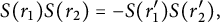 $$ \begin{align*}S(r_1)S(r_2) = - S(r_1^{\prime})S(r_2^{\prime}),\end{align*} $$
(2) if $r_1*r_2$
is a horizontal annulus, then
$r_1*r_2$
is a horizontal annulus, then $S(r_1)S(r_2)=1,$
and (3) if
$S(r_1)S(r_2)=1,$
and (3) if $r_1*r_2$
is a vertical annulus, then
$r_1*r_2$
is a vertical annulus, then $S(r_1)S(r_2)=-1.$
An extended sign assignment is a function $S:\operatorname {\mathrm {Rect}}^{*}(\mathbb {G})\rightarrow \{-1, 1\}$
satisfying properties (2) and (3) above, and also (1’): if there exists a domain
$S:\operatorname {\mathrm {Rect}}^{*}(\mathbb {G})\rightarrow \{-1, 1\}$
satisfying properties (2) and (3) above, and also (1’): if there exists a domain $\psi $
such that
$\psi $
such that $\psi = r_1*r_2 = r_1^{\prime }*r_2^{\prime }$
for
$\psi = r_1*r_2 = r_1^{\prime }*r_2^{\prime }$
for $r_1, r_2, r_1^{\prime }, r_2^{\prime }\in \operatorname {\mathrm {Rect}}^{*}(\mathbb {G}),$
then
$r_1, r_2, r_1^{\prime }, r_2^{\prime }\in \operatorname {\mathrm {Rect}}^{*}(\mathbb {G}),$
then
 $$ \begin{align*}S(r_1)S(r_2) = - S(r_1^{\prime})S(r_2^{\prime}).\end{align*} $$
Definition 5.2 For $\psi \in \pi (\mathbf {x}, \mathbf {z}),$
let
$\psi \in \pi (\mathbf {x}, \mathbf {z}),$
let $D(\psi )$
be the set of decompositions of
$D(\psi )$
be the set of decompositions of $\psi $
into two rectangles, and
$\psi $
into two rectangles, and $D^{*}(\psi )$
the set of decompositions of
$D^{*}(\psi )$
the set of decompositions of $\psi $
into one rectangle and one long rectangle (in either order). For
$\psi $
into one rectangle and one long rectangle (in either order). For $d=r_1*r_2\in D(\psi )\cup D^{*}(\psi ),$
define the sign
$d=r_1*r_2\in D(\psi )\cup D^{*}(\psi ),$
define the sign $S(d)$
to be
$S(d)$
to be $S(r_1)*S(r_2).$
Remark 5.3 Note that if $r_1$
and
$r_1$
and $r_2$
are two rectangles with
$r_2$
are two rectangles with $r_1\in \operatorname {\mathrm {Rect}}(\mathbf {x}, \mathbf {y})$
and
$r_1\in \operatorname {\mathrm {Rect}}(\mathbf {x}, \mathbf {y})$
and $r_2\in \operatorname {\mathrm {Rect}}(\mathbf {z}, \mathbf {w}),$
it is possible that
$r_2\in \operatorname {\mathrm {Rect}}(\mathbf {z}, \mathbf {w}),$
it is possible that $r_1$
and
$r_1$
and $r_2$
have the same support but
$r_2$
have the same support but $S(r_1)\neq S(r_2).$
It is therefore important to emphasize that S is a function of the domain, initial, and final grid states.
$S(r_1)\neq S(r_2).$
It is therefore important to emphasize that S is a function of the domain, initial, and final grid states.
Note further that by the definition of our sign assignments, the proofs of Lemmas 4.2 and 4.3 extend to prove the following slightly stronger statement.
Lemma 5.4 Under the assumptions of Lemma 4.2 or Lemma 4.3, the two decompositions of $\psi $
resulting from those lemmas have opposite signs.
$\psi $
resulting from those lemmas have opposite signs.
Given a sign assignment, we may define a new chain complex over the integers. Let $\mathit {GCL}^-(\mathbb {G}; \mathbb {Z})$
be the free
$\mathit {GCL}^-(\mathbb {G}; \mathbb {Z})$
be the free $\mathbb {Z}[V_1,\dots , V_n, v]$
-module generated by the grid states of
$\mathbb {Z}[V_1,\dots , V_n, v]$
-module generated by the grid states of $\mathbb {G},$
with multiplication by each
$\mathbb {G},$
with multiplication by each $V_i$
homogeneous of bigrading
$V_i$
homogeneous of bigrading $(-2, -1),$
and multiplication by v homogeneous of bigrading
$(-2, -1),$
and multiplication by v homogeneous of bigrading $(2, 0).$
Define the differential as follows on grid states, extending by linearity:
$(2, 0).$
Define the differential as follows on grid states, extending by linearity:
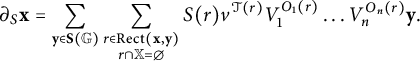 $$ \begin{align*}\partial_S\mathbf{x}= \sum_{\mathbf{y}\in\mathbf{S}(\mathbb{G})}\sum_{\substack{ r\in\operatorname{\mathrm{Rect}}(\mathbf{x}, \mathbf{y}) \\ r\cap\mathbb{X} = \emptyset\\}} S(r)v^{\mathcal{T}(r)}V_1^{O_1(r)}\dots V_n^{O_n(r)}\mathbf{y}.\end{align*} $$
Proposition 5.5 $\partial _{S}^2=0$
for any sign assignment
$\partial _{S}^2=0$
for any sign assignment $S.$
$S.$
Proof By expanding out definitions, we see
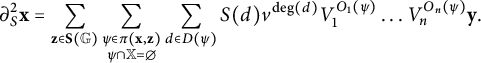 $$ \begin{align*}\partial_S^2\mathbf{x} = \sum_{\mathbf{z}\in\mathbf{S}(\mathbb{G})}\sum_{\substack{\psi\in\pi(\mathbf{x}, \mathbf{z})\\ \psi\cap\mathbb{X} = \emptyset\\}} \sum_{d\in D(\psi)}S(d)v^{\deg(d)}V_1^{O_1(\psi)}\dots V_n^{O_n(\psi)}\mathbf{y}.\end{align*} $$
Hence, it is sufficient to show that domains $\psi \in \pi (\mathbf {x}, \mathbf {z})$
with
$\psi \in \pi (\mathbf {x}, \mathbf {z})$
with $\lvert D(\psi )\rvert>0$
have exactly two decompositions
$\lvert D(\psi )\rvert>0$
have exactly two decompositions $d\in D(\psi )$
with equal degree and opposite signs.
$d\in D(\psi )$
with equal degree and opposite signs.
If $\lvert \mathbf {x} -\mathbf {x}\cap \mathbf {z}\rvert = 4$
or
$\lvert \mathbf {x} -\mathbf {x}\cap \mathbf {z}\rvert = 4$
or $\lvert \mathbf {x} -\mathbf {x}\cap \mathbf {z}\rvert = 3,$
then Lemma 5.4 tells us immediately that any
$\lvert \mathbf {x} -\mathbf {x}\cap \mathbf {z}\rvert = 3,$
then Lemma 5.4 tells us immediately that any $\psi \in \pi (\mathbf {x}, \mathbf {z})$
with
$\psi \in \pi (\mathbf {x}, \mathbf {z})$
with $\lvert D(\psi )\rvert>0$
has exactly two decompositions
$\lvert D(\psi )\rvert>0$
has exactly two decompositions $d\in D(\psi )$
with equal degree and opposite signs.
$d\in D(\psi )$
with equal degree and opposite signs.
The last case is $\mathbf {x} = \mathbf {z}.$
Lemma 4.4 tells us that in this case,
$\mathbf {x} = \mathbf {z}.$
Lemma 4.4 tells us that in this case, $\psi $
is an annulus, hence
$\psi $
is an annulus, hence $\psi \cap \mathbb {X}\neq \emptyset ,$
so this also contributes 0 to the equation.
$\psi \cap \mathbb {X}\neq \emptyset ,$
so this also contributes 0 to the equation.
Let $\mathit {GHL}^-_S(\mathbb {G}; \mathbb {Z})$
be the homology of this chain complex. We will eventually see that the
$\mathit {GHL}^-_S(\mathbb {G}; \mathbb {Z})$
be the homology of this chain complex. We will eventually see that the $V_i$
are homotopic to each other, hence calling the induced multiplication
$V_i$
are homotopic to each other, hence calling the induced multiplication $U,$
we get
$U,$
we get $\mathit {GHL}^-_S(\mathbb {G}; \mathbb {Z})$
is a bigraded
$\mathit {GHL}^-_S(\mathbb {G}; \mathbb {Z})$
is a bigraded $\mathbb {Z}[U, v]$
-module.
$\mathbb {Z}[U, v]$
-module.
We wish to prove the following theorem, which is an analog of the invariance of ordinary grid homology over the integers.
Theorem 5.6 For each grid diagram, there exists a sign assignment; furthermore, all sign assignments produce isomorphic homology $\mathit {GHL}^-_S(\mathbb {G}; \mathbb {Z}).$
Moreover, the bigraded
$\mathit {GHL}^-_S(\mathbb {G}; \mathbb {Z}).$
Moreover, the bigraded $\mathbb {Z}[U, v]$
-module isomorphism type of
$\mathbb {Z}[U, v]$
-module isomorphism type of $\mathit {GHL}^-_S(\mathbb {G}; \mathbb {Z})$
is a knot invariant.
$\mathit {GHL}^-_S(\mathbb {G}; \mathbb {Z})$
is a knot invariant.
We divide the proof of this theorem into several steps. First, we lift existence and uniqueness of sign assignments for grid homology to our situation, which is rather simple.
Lemma 5.7 For each grid diagram, there exists a sign assignment; furthermore, all sign assignments produce isomorphic homology $\mathit {GHL}^-_S(\mathbb {G}; \mathbb {Z}).$
Proof The existence of a sign assignment follows immediately from [Reference Ozsváth, Stipcisz and Szabó5, Theorem 15.1.5]. Their proof of this theorem also shows that for any two sign assignments $S_1$
and
$S_1$
and $S_2,$
there exists a function
$S_2,$
there exists a function $g:\mathbf {S}(\mathbb {G})\rightarrow \{-1, 1\}$
such that
$g:\mathbf {S}(\mathbb {G})\rightarrow \{-1, 1\}$
such that $S_2(r) = g(\mathbf {x})S_1(r)g(\mathbf {y})$
for each
$S_2(r) = g(\mathbf {x})S_1(r)g(\mathbf {y})$
for each $r\in \operatorname {\mathrm {Rect}}(\mathbf {x}, \mathbf {y}).$
Hence, we may define a
$r\in \operatorname {\mathrm {Rect}}(\mathbf {x}, \mathbf {y}).$
Hence, we may define a $\mathbb {Z}[V_1,\dots , V_n, v]$
-module homomorphism from
$\mathbb {Z}[V_1,\dots , V_n, v]$
-module homomorphism from $(\mathit {GCL}^-(\mathbb {G}; \mathbb {Z}), \partial _{S_1})$
to
$(\mathit {GCL}^-(\mathbb {G}; \mathbb {Z}), \partial _{S_1})$
to $(\mathit {GCL}^-(\mathbb {G}; \mathbb {Z}), \partial _{S_2})$
by
$(\mathit {GCL}^-(\mathbb {G}; \mathbb {Z}), \partial _{S_2})$
by $\mathbf {x}\mapsto g(\mathbf {x})\mathbf {x}.$
It is immediate that this is a chain map and an isomorphism of
$\mathbf {x}\mapsto g(\mathbf {x})\mathbf {x}.$
It is immediate that this is a chain map and an isomorphism of $\mathbb {Z}[V_1,\dots , V_n, v]$
-modules, and this suffices for the proof. (This is an analog of the map defined in [Reference Ozsváth, Stipcisz and Szabó5, Proposition 15.1.10].)
$\mathbb {Z}[V_1,\dots , V_n, v]$
-modules, and this suffices for the proof. (This is an analog of the map defined in [Reference Ozsváth, Stipcisz and Szabó5, Proposition 15.1.10].)
Next, we show that the $V_i$
are homotopic. For this, we require a lemma about extended sign assignments, and some definitions. For any long rectangle
$V_i$
are homotopic. For this, we require a lemma about extended sign assignments, and some definitions. For any long rectangle $r\in \operatorname {\mathrm {Rect}}^{*}(\mathbf {x}, \mathbf {y}),$
deleting an annulus leaves a rectangle
$r\in \operatorname {\mathrm {Rect}}^{*}(\mathbf {x}, \mathbf {y}),$
deleting an annulus leaves a rectangle $r'\in \operatorname {\mathrm {Rect}}^{*}(\mathbf {x},\mathbf {y})$
which we will call the associated short rectangle.
$r'\in \operatorname {\mathrm {Rect}}^{*}(\mathbf {x},\mathbf {y})$
which we will call the associated short rectangle.
Lemma 5.8 Each sign assignment $S:\operatorname {\mathrm {Rect}}(\mathbb {G})\rightarrow \{-1, 1\}$
may be extended to an extended sign assignment, such that if
$S:\operatorname {\mathrm {Rect}}(\mathbb {G})\rightarrow \{-1, 1\}$
may be extended to an extended sign assignment, such that if $r\in \operatorname {\mathrm {Rect}}^{*}(\mathbf {x},\mathbf {y})$
is long and
$r\in \operatorname {\mathrm {Rect}}^{*}(\mathbf {x},\mathbf {y})$
is long and $r'\in \operatorname {\mathrm {Rect}}^{*}(\mathbf {x},\mathbf {y})$
is its associated short rectangle, then
$r'\in \operatorname {\mathrm {Rect}}^{*}(\mathbf {x},\mathbf {y})$
is its associated short rectangle, then $S(r) = S(r').$
Proof We use the notation of [Reference Ozsváth, Stipcisz and Szabó5, Chapter 15]. Let $\tilde {\mathfrak {S}}_n$
denote the spin extension of the symmetric group on n letters (see [Reference Ozsváth, Stipcisz and Szabó5, Section 15.2]), and let
$\tilde {\mathfrak {S}}_n$
denote the spin extension of the symmetric group on n letters (see [Reference Ozsváth, Stipcisz and Szabó5, Section 15.2]), and let $\tilde {T}$
denote the set of lifts of transpositions in
$\tilde {T}$
denote the set of lifts of transpositions in $\mathfrak {S}_n$
; these are indexed by ordered pairs of distinct integers in
$\mathfrak {S}_n$
; these are indexed by ordered pairs of distinct integers in $\{1,\dots , n\}$
and denoted by
$\{1,\dots , n\}$
and denoted by $\tilde {\tau }_{i,j}$
for
$\tilde {\tau }_{i,j}$
for $i\neq j.$
Here,
$i\neq j.$
Here, $\tilde {\tau }_{i,j}$
and
$\tilde {\tau }_{i,j}$
and $\tilde {\tau }_{j,i}$
are the two lifts of the permutation
$\tilde {\tau }_{j,i}$
are the two lifts of the permutation $(i j)\in \mathfrak {S}_n.$
Also,
$(i j)\in \mathfrak {S}_n.$
Also, $z\neq 1\in \tilde {{\mathfrak {S}}}_n$
is the other lift of the identity
$z\neq 1\in \tilde {{\mathfrak {S}}}_n$
is the other lift of the identity $1\in \mathfrak {S}_n.$
Let $\tilde {\tau }:\operatorname {\mathrm {Rect}}^{*}(\mathbb {G})\rightarrow \tilde {T}$
be the map sending
$\tilde {\tau }:\operatorname {\mathrm {Rect}}^{*}(\mathbb {G})\rightarrow \tilde {T}$
be the map sending $r\in \operatorname {\mathrm {Rect}}^{*}(\mathbb {G})$
to
$r\in \operatorname {\mathrm {Rect}}^{*}(\mathbb {G})$
to $\tilde {\tau }_{i,j}$
where the southwest corner of the associated short rectangle
$\tilde {\tau }_{i,j}$
where the southwest corner of the associated short rectangle $r'$
is on
$r'$
is on $\beta _i$
and the northeast corner of r is on
$\beta _i$
and the northeast corner of r is on $\beta _i$
. We wish to show the following three conditions hold:
$\beta _i$
. We wish to show the following three conditions hold:
-
• If there is a region
$\psi $
with two decompositions
$\psi = r_1*r_2 = r_1^{\prime }*r_2^{\prime }$
for
$r_1, r_2, r_1^{\prime }, r_2^{\prime }\in \operatorname {\mathrm {Rect}}^{*}(\mathbb {G})$
with at most one of
$r_1, r_2$
long, then
$$ \begin{align*}\tilde{\tau}(r_1)\cdot\tilde{\tau}(r_2) = z \cdot\tilde{\tau}(r_1^{\prime})\cdot\tilde{\tau}(r_2^{\prime}).\end{align*} $$
-
• If
$r_1*r_2$
forms a horizontal annulus of multiplicity 1, then
$$ \begin{align*}\tilde{\tau}(r_1)\cdot\tilde{\tau}(r_2) = 1.\end{align*} $$
-
• If
$r_1*r_2$
forms a vertical annulus of multiplicity 1, then
$$ \begin{align*}\tilde{\tau}(r_1)\cdot\tilde{\tau}(r_2) = z.\end{align*} $$


Assuming for now that these three conditions hold, we will demonstrate the existence of the extension of our sign assignment $S.$
For each grid state
$S.$
For each grid state $\mathbf {x},$
let
$\mathbf {x},$
let $\sigma _{\mathbf {x}}\in \mathfrak {S}_n$
be the corresponding permutation which is determined uniquely by
$\sigma _{\mathbf {x}}\in \mathfrak {S}_n$
be the corresponding permutation which is determined uniquely by $\alpha _i\cap \beta _{\sigma _{\mathbf {x}}(i)}\in \mathbf {x}.$
[Reference Ozsváth, Stipcisz and Szabó5, Section 15.2] proves that every sign assignment, in particular
$\alpha _i\cap \beta _{\sigma _{\mathbf {x}}(i)}\in \mathbf {x}.$
[Reference Ozsváth, Stipcisz and Szabó5, Section 15.2] proves that every sign assignment, in particular $S,$
is given, for
$S,$
is given, for $r\in \operatorname {\mathrm {Rect}}(\mathbf {x}, \mathbf {y})$
, as
$r\in \operatorname {\mathrm {Rect}}(\mathbf {x}, \mathbf {y})$
, as $S(r) = \tilde {\tau }(r)^{-1}\gamma (\sigma _{\mathbf {x}}^{-1})\gamma (\sigma _{\mathbf {y}}),$
for some section of the spin extension
$S(r) = \tilde {\tau }(r)^{-1}\gamma (\sigma _{\mathbf {x}}^{-1})\gamma (\sigma _{\mathbf {y}}),$
for some section of the spin extension $\gamma :\mathfrak {S}_n\rightarrow \tilde {\mathfrak {S}}_n.$
Furthermore, the proof of [Reference Ozsváth, Stipcisz and Szabó5, Proposition 15.2.12] tells us that if S is extended to long rectangles by the same formula,
$\gamma :\mathfrak {S}_n\rightarrow \tilde {\mathfrak {S}}_n.$
Furthermore, the proof of [Reference Ozsváth, Stipcisz and Szabó5, Proposition 15.2.12] tells us that if S is extended to long rectangles by the same formula, $S(r) = \tilde {\tau }(r)^{-1}\gamma (\sigma _{\mathbf {x}}^{-1})\gamma (\sigma _{\mathbf {y}}),$
then S will satisfy the conditions of an extended sign assignment if
$S(r) = \tilde {\tau }(r)^{-1}\gamma (\sigma _{\mathbf {x}}^{-1})\gamma (\sigma _{\mathbf {y}}),$
then S will satisfy the conditions of an extended sign assignment if $\tilde {\tau }$
obeys the three above conditions.
$\tilde {\tau }$
obeys the three above conditions.
Thus, it is sufficient to show that $\tilde {\tau }$
obeys the three above conditions. The second and third are immediate from [Reference Ozsváth, Stipcisz and Szabó5, Section 15.2] since they do not apply to long rectangles. The first condition is immediate in the case when both decompositions of
$\tilde {\tau }$
obeys the three above conditions. The second and third are immediate from [Reference Ozsváth, Stipcisz and Szabó5, Section 15.2] since they do not apply to long rectangles. The first condition is immediate in the case when both decompositions of $\psi $
involve one long rectangle, since deleting an annulus from
$\psi $
involve one long rectangle, since deleting an annulus from $\psi $
and in turn from each of the long rectangles does not change the map
$\psi $
and in turn from each of the long rectangles does not change the map $\tilde {\tau }$
and this condition now follows from the equivalent condition for not long rectangles.
$\tilde {\tau }$
and this condition now follows from the equivalent condition for not long rectangles.
Finally, we must show this condition is true when one decomposition, $r_1*r_2,$
of
$r_1*r_2,$
of $\psi $
involves a long rectangle and the other,
$\psi $
involves a long rectangle and the other, $r_1^{\prime }*r_2^{\prime },$
does not. Say that
$r_1^{\prime }*r_2^{\prime },$
does not. Say that $r_1$
is long and
$r_1$
is long and $r_1^{\prime }$
has width one. This reduces to eight cases, corresponding to whether
$r_1^{\prime }$
has width one. This reduces to eight cases, corresponding to whether $r_1$
horizontal or vertical, and whether the multiplicity 2 portion of
$r_1$
horizontal or vertical, and whether the multiplicity 2 portion of $\psi $
is in the Southwest, Southeast, Northwest, or Northeast corner of
$\psi $
is in the Southwest, Southeast, Northwest, or Northeast corner of $r_2^{\prime }.$
For each, it is a simple computation involving the relations among the members of
$r_2^{\prime }.$
For each, it is a simple computation involving the relations among the members of $\tilde {T}.$
Definition 5.9 We define the sign-refined homotopy operator as follows. Let $X_i\in \mathbb {X}$
share a row with
$X_i\in \mathbb {X}$
share a row with $O_i$
. Then, define the function
$O_i$
. Then, define the function
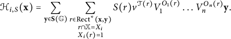 $$ \begin{align*}\mathcal{H}_{i, S}(\mathbf{x}) = \sum_{\mathbf{y}\in\mathbf{S}(\mathbb{G})}\sum_{\substack{ r\in\operatorname{\mathrm{Rect}}^{*}(\mathbf{x}, \mathbf{y})\\ r\cap\mathbb{X} = X_i \\ X_i(r)=1\\}} S(r)v^{\mathcal{T}(r)}V_1^{O_1(r)}\dots V_n^{O_n(r)}\mathbf{y}.\end{align*} $$
Proposition 5.10 Suppose $X_i$
shares a column with
$X_i$
shares a column with $O_j.$
Then following equation holds:
$O_j.$
Then following equation holds:
 $$ \begin{align*}\mathcal{H}_{i, S}\circ\partial_S + \partial_S\circ\mathcal{H}_{i, S} = V_i - V_j.\end{align*} $$
Proof By expanding out definitions, we see the left-hand side is given as
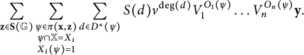 $$ \begin{align*}\sum_{\mathbf{z}\in\mathbf{S}(\mathbb{G})}\sum_{\substack{\psi\in\pi(\mathbf{x}, \mathbf{z})\\ \psi\cap\mathbb{X} = X_i \\ X_i(\psi)=1\\}} \sum_{d\in D^{*}(\psi)}S(d)v^{\deg(d)}V_1^{O_1(\psi)}\dots V_n^{O_n(\psi)}\mathbf{y}.\end{align*} $$
If $\lvert \mathbf {x} -\mathbf {x}\cap \mathbf {z}\rvert = 4$
or
$\lvert \mathbf {x} -\mathbf {x}\cap \mathbf {z}\rvert = 4$
or $\lvert \mathbf {x} -\mathbf {x}\cap \mathbf {z}\rvert = 3,$
then Lemma 5.4 tells us immediately that any
$\lvert \mathbf {x} -\mathbf {x}\cap \mathbf {z}\rvert = 3,$
then Lemma 5.4 tells us immediately that any $\psi \in \pi (\mathbf {x}, \mathbf {z})$
with
$\psi \in \pi (\mathbf {x}, \mathbf {z})$
with $\lvert D(\psi )\rvert>0$
has exactly two decompositions
$\lvert D(\psi )\rvert>0$
has exactly two decompositions $d\in D(\psi )$
with equal degree and opposite signs. Hence, all such
$d\in D(\psi )$
with equal degree and opposite signs. Hence, all such $\psi $
contribute zero to the above sum.
$\psi $
contribute zero to the above sum.
The last case is $\mathbf {x} = \mathbf {z}.$
Lemma 4.4 tells us that in this case,
$\mathbf {x} = \mathbf {z}.$
Lemma 4.4 tells us that in this case, $\psi $
is an annulus, hence
$\psi $
is an annulus, hence $\psi \cap \mathbb {X}=X_i$
has precisely two solutions, a horizontal thin annulus and a vertical thin annulus. (The multiplicities of these annuli must be 1 since
$\psi \cap \mathbb {X}=X_i$
has precisely two solutions, a horizontal thin annulus and a vertical thin annulus. (The multiplicities of these annuli must be 1 since $X_i(\psi )=1.$
) The horizontal thin annulus contributes
$X_i(\psi )=1.$
) The horizontal thin annulus contributes $V_i$
and the vertical thin annulus contributes
$V_i$
and the vertical thin annulus contributes $-V_j.$
Proposition 5.11 For any $k, l,$
we have
$k, l,$
we have $V_k$
and
$V_k$
and $V_l$
are chain homotopic.
$V_l$
are chain homotopic.
Proof The above proposition shows that $V_i$
and
$V_i$
and $V_j$
are chain homotopic whenever
$V_j$
are chain homotopic whenever $O_i$
and
$O_i$
and $O_j$
are consecutive O-markings as we traverse the knot. Since the knot has one component, each
$O_j$
are consecutive O-markings as we traverse the knot. Since the knot has one component, each $O_k$
and
$O_k$
and $O_l$
are both members of a finite sequence of consecutive O-markings, which suffices for the proof.
$O_l$
are both members of a finite sequence of consecutive O-markings, which suffices for the proof.
The remainder of the proof of invariance of the sign-refined homology $\mathit {GHL}^-_S(\mathbb {G};\mathbb {Z})$
is to show it is a knot invariant. By Theorem 2.10, it suffices to show that this homology is unchanged under commutations and switches, and also under (de)-stabilizations of type X:
$\mathit {GHL}^-_S(\mathbb {G};\mathbb {Z})$
is to show it is a knot invariant. By Theorem 2.10, it suffices to show that this homology is unchanged under commutations and switches, and also under (de)-stabilizations of type X: $SW.$
$SW.$
5.1 Commutation and switch invariance
First, we show this for the commutations and switches; we model our arguments off of those in [Reference Ozsváth, Stipcisz and Szabó5, Section 15.3]. As in Section 3.1, we take two grid diagrams $\mathbb {G}$
and
$\mathbb {G}$
and $\mathbb {G}'$
related by a commutation or switch and superimpose them; we borrow here the notation from that section. We will do the computations below for a column commutation or switch; a row commutation or switch proceeds identically. Very concretely, the goal of this section is to prove the following theorem:
$\mathbb {G}'$
related by a commutation or switch and superimpose them; we borrow here the notation from that section. We will do the computations below for a column commutation or switch; a row commutation or switch proceeds identically. Very concretely, the goal of this section is to prove the following theorem:
Theorem 5.12 If two grid diagrams $\mathbb {G}$
and
$\mathbb {G}$
and $\mathbb {G}'$
as above differ by a column commutation or switch, then
$\mathbb {G}'$
as above differ by a column commutation or switch, then $\mathit {GCL}^-_S(\mathbb {G};\mathbb {Z})$
and
$\mathit {GCL}^-_S(\mathbb {G};\mathbb {Z})$
and $\mathit {GCL}^-_S(\mathbb {G}';\mathbb {Z})$
are quasi-isomorphic chain complexes.
$\mathit {GCL}^-_S(\mathbb {G}';\mathbb {Z})$
are quasi-isomorphic chain complexes.
Again, we recall that by Remark 3.9, we may guarantee that each bigon bounded by $\beta _i$
and
$\beta _i$
and $\gamma _i$
contains at least one
$\gamma _i$
contains at least one $\mathbb {X}$
-marking inside.
$\mathbb {X}$
-marking inside.
First, we must define pentagon and hexagon maps; the pentagon maps will provide the quasi-isomorphism and the hexagon map will be the relevant homotopy operator. For this, we need signs for pentagons and hexagons.
Definition 5.13 For a pentagon $p\in \operatorname {\mathrm {Pent}}^{*}(\mathbf {x}, \mathbf {y}'),$
let P be its associated rectangular domain. We define the sign of p as follows:
$p\in \operatorname {\mathrm {Pent}}^{*}(\mathbf {x}, \mathbf {y}'),$
let P be its associated rectangular domain. We define the sign of p as follows:
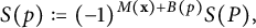 $$ \begin{align*}S(p) := (-1)^{M(\mathbf{x})+B(p)}S(P),\end{align*} $$
where $B(p)$
is 1 if p lies to the left of
$B(p)$
is 1 if p lies to the left of $\beta _i$
and 0 if p lies to the right of
$\beta _i$
and 0 if p lies to the right of $\beta _i.$
Similarly, for
$\beta _i.$
Similarly, for $p\in \operatorname {\mathrm {Pent}}^{*}(\mathbf {x}', \mathbf {y}),$
let P be its associated rectangular domain. We define the sign of p as follows:
$p\in \operatorname {\mathrm {Pent}}^{*}(\mathbf {x}', \mathbf {y}),$
let P be its associated rectangular domain. We define the sign of p as follows:
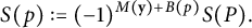 $$ \begin{align*}S(p) := (-1)^{M(\mathbf{y})+B(p)}S(P).\end{align*} $$
For a hexagon $h\in \operatorname {\mathrm {Hex}}^{*}(\mathbf {x}, \mathbf {y}),$
let H be its associated rectangular domain. We define the sign of h simply as
$h\in \operatorname {\mathrm {Hex}}^{*}(\mathbf {x}, \mathbf {y}),$
let H be its associated rectangular domain. We define the sign of h simply as $S(h) := S(H).$
Definition 5.14 The pentagon map $P_S:\mathit {GCL}^-_S(\mathbb {G};\mathbb {Z})\rightarrow \mathit {GCL}^-_S(\mathbb {G}';\mathbb {Z})$
is defined as
$P_S:\mathit {GCL}^-_S(\mathbb {G};\mathbb {Z})\rightarrow \mathit {GCL}^-_S(\mathbb {G}';\mathbb {Z})$
is defined as
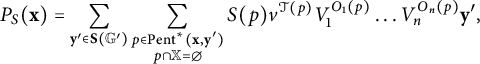 $$ \begin{align*} P_S(\mathbf{x}) = \sum_{\mathbf{y}'\in\mathbf{S}(\mathbb{G}')}\sum_{\substack{p\in\operatorname{\mathrm{Pent}}^{*}(\mathbf{x}, \mathbf{y}')\\ p\cap\mathbb{X} = \emptyset\\}} S(p)v^{\mathcal{T}(p)}V_1^{O_1(p)}\dots V_n^{O_n(p)}\mathbf{y}', \end{align*} $$
and we define a similar map $P_S^{\prime }:\mathit {GCL}^-_S(\mathbb {G}';\mathbb {Z})\rightarrow \mathit {GCL}^-_S(\mathbb {G};\mathbb {Z})$
by
$P_S^{\prime }:\mathit {GCL}^-_S(\mathbb {G}';\mathbb {Z})\rightarrow \mathit {GCL}^-_S(\mathbb {G};\mathbb {Z})$
by
 $$ \begin{align*} P_S^{\prime}(\mathbf{x}') = \sum_{\mathbf{y}\in\mathbf{S}(\mathbb{G})}\sum_{\substack{p\in\operatorname{\mathrm{Pent}}^{*}(\mathbf{x}', \mathbf{y})\\ p\cap\mathbb{X} = \emptyset\\}} S(p)v^{\mathcal{T}(p)}V_1^{O_1(p)}\dots V_n^{O_n(p)}\mathbf{y}. \end{align*} $$
The hexagon map $H_S:\mathit {GCL}^-_S(\mathbb {G};\mathbb {Z})\rightarrow \mathit {GCL}^-_S(\mathbb {G};\mathbb {Z})$
is defined as
$H_S:\mathit {GCL}^-_S(\mathbb {G};\mathbb {Z})\rightarrow \mathit {GCL}^-_S(\mathbb {G};\mathbb {Z})$
is defined as
 $$ \begin{align*} H_S(\mathbf{x}) = \sum_{\mathbf{y}\in\mathbf{S}(\mathbb{G})}\sum_{\substack{h\in\operatorname{\mathrm{Hex}}^{*}(\mathbf{x}, \mathbf{y})\\ h\cap\mathbb{X} = \emptyset\\}} S(h)v^{\mathcal{T}(h)}V_1^{O_1(h)}\dots V_n^{O_n(h)}\mathbf{y}. \end{align*} $$
Proposition 5.15 The pentagon map $P_S$
is a bigraded quasi-isomorphism.
$P_S$
is a bigraded quasi-isomorphism.
Proof First, we show $P_S$
is bigraded. This is an immediate consequence of the relative formulas for Maslov and Alexander gradings as well as Lemma 4.7.
$P_S$
is bigraded. This is an immediate consequence of the relative formulas for Maslov and Alexander gradings as well as Lemma 4.7.
Next, we show $P_S$
is a chain map; this amounts to showing that
$P_S$
is a chain map; this amounts to showing that $P_S\circ \partial _S-\partial _S\circ P_S = 0.$
For a domain
$P_S\circ \partial _S-\partial _S\circ P_S = 0.$
For a domain $\psi \in \pi (\mathbf {x}, \mathbf {z}'),$
let
$\psi \in \pi (\mathbf {x}, \mathbf {z}'),$
let $D_{pr}(\psi )$
be the set of all decompositions of
$D_{pr}(\psi )$
be the set of all decompositions of $\psi $
as a (possibly long) pentagon and a (not long) rectangle in that order, and
$\psi $
as a (possibly long) pentagon and a (not long) rectangle in that order, and $D_{rp}(\psi )$
the reverse. Expanding out the equation, we wish to show
$D_{rp}(\psi )$
the reverse. Expanding out the equation, we wish to show
 $$ \begin{align*} & \sum_{\mathbf{z}'\in\mathbf{S}(\mathbb{G}')}\sum_{\substack{\psi\in\pi(\mathbf{x}, \mathbf{z}')\\ \psi\cap\mathbb{X} = \emptyset\\}} \sum_{d\in D_{pr}(\psi)} S(d)v^{\deg(d)}V_1^{O_1(\psi)}\dots V_n^{O_n(\psi)}\mathbf{z}'\\[2pt]& \quad = \sum_{\mathbf{z}'\in\mathbf{S}(\mathbb{G}')}\sum_{\substack{\psi\in\pi(\mathbf{x}, \mathbf{z}')\\ \psi\cap\mathbb{X} = \emptyset\\}} \sum_{d\in D_{rp}(\psi)} S(d) v^{\deg(d)}V_1^{O_1(\psi)}\dots V_n^{O_n(\psi)}\mathbf{z}'. \end{align*} $$
In this case, we see immediately that $\lvert \mathbf {x} - \mathbf {x}\cap \mathbf {z}'\rvert $
could be 3, 4, or 1. If it is 4, then the proof of Corollary 4.10 tells us that any
$\lvert \mathbf {x} - \mathbf {x}\cap \mathbf {z}'\rvert $
could be 3, 4, or 1. If it is 4, then the proof of Corollary 4.10 tells us that any $\psi $
with
$\psi $
with $\lvert D_{rp}(\psi )\cup D_{pr}(\psi )\rvert \geq 1$
has exactly two decompositions
$\lvert D_{rp}(\psi )\cup D_{pr}(\psi )\rvert \geq 1$
has exactly two decompositions $r*p$
and
$r*p$
and $p^{\prime }*r'$
of equal degree corresponding to the two rectangular decompositions of
$p^{\prime }*r'$
of equal degree corresponding to the two rectangular decompositions of $\Psi .$
To show the contribution of
$\Psi .$
To show the contribution of $\psi $
is equal on both sides of the equation, it is sufficient to show that the signs of these two decompositions is equal. By the definition of a sign assignment, and the decompositions of
$\psi $
is equal on both sides of the equation, it is sufficient to show that the signs of these two decompositions is equal. By the definition of a sign assignment, and the decompositions of $\Psi ,$
we see that
$\Psi ,$
we see that
 $$ \begin{align*} S(r)S(R(p)) = -S(R(p'))S(r'). \end{align*} $$
Since the pentagons p and $p'$
have initial grid states of opposite parity and clearly
$p'$
have initial grid states of opposite parity and clearly $B(p)=B(p'),$
as they have the same support, the signs
$B(p)=B(p'),$
as they have the same support, the signs $S(r*p)$
and
$S(r*p)$
and $S(p^{\prime }*r')$
are indeed equal.
$S(p^{\prime }*r')$
are indeed equal.
Next, suppose $\lvert \mathbf {x} - \mathbf {x}\cap \mathbf {z}'\rvert =3.$
Then, as in the proof of Corollary 4.10, any
$\lvert \mathbf {x} - \mathbf {x}\cap \mathbf {z}'\rvert =3.$
Then, as in the proof of Corollary 4.10, any $\psi $
with
$\psi $
with $\lvert D_{rp}(\psi )\cup D_{pr}(\psi )\rvert \geq 1$
has exactly two decompositions of equal degree corresponding to the two rectangular decompositions of
$\lvert D_{rp}(\psi )\cup D_{pr}(\psi )\rvert \geq 1$
has exactly two decompositions of equal degree corresponding to the two rectangular decompositions of $\Psi .$
The proof of Corollary 4.10 gives us two cases. First, that these two decompositions correspond to different decompositions of $\Psi .$
Here, the two associated rectangular decompositions have opposite signs. However, the B-value of the pentagons in each decomposition is obviously equal, and the Maslov initial grid states of the pentagons in each decomposition differ in parity if and only if one decomposition is in
$\Psi .$
Here, the two associated rectangular decompositions have opposite signs. However, the B-value of the pentagons in each decomposition is obviously equal, and the Maslov initial grid states of the pentagons in each decomposition differ in parity if and only if one decomposition is in $D_{rp}(\psi )$
and the other is in
$D_{rp}(\psi )$
and the other is in $D_{pr}(\psi ).$
Hence,
$D_{pr}(\psi ).$
Hence, $\psi $
contributes equally to both sides of the above equation in this case.
$\psi $
contributes equally to both sides of the above equation in this case.
Otherwise, these two decompositions correspond to the same rectangular decomposition of $\Psi ,$
in which case the decompositions are of the form
$\Psi ,$
in which case the decompositions are of the form $r*p$
and
$r*p$
and $p^{\prime }*r'$
, and
$p^{\prime }*r'$
, and $b(p)=-b(p'),$
so
$b(p)=-b(p'),$
so $\psi $
also contributes equally to both sides of the above equation in this case.
$\psi $
also contributes equally to both sides of the above equation in this case.
The final case is when $\lvert \mathbf {x} - \mathbf {x}\cap \mathbf {z}'\rvert =1.$
Then, the associated rectangular domain is an annulus, and must therefore be thin to avoid intersection with
$\lvert \mathbf {x} - \mathbf {x}\cap \mathbf {z}'\rvert =1.$
Then, the associated rectangular domain is an annulus, and must therefore be thin to avoid intersection with $\mathbb {X}$
; furthermore, the condition that each bigon contains an X-marking prevents this annulus from having multiplicity 2. Hence, the degrees of all decompositions must be 0, and the remainder of the proof proceeds exactly as in [Reference Ozsváth, Stipcisz and Szabó5, Lemma 15.3.3].
$\mathbb {X}$
; furthermore, the condition that each bigon contains an X-marking prevents this annulus from having multiplicity 2. Hence, the degrees of all decompositions must be 0, and the remainder of the proof proceeds exactly as in [Reference Ozsváth, Stipcisz and Szabó5, Lemma 15.3.3].
By identical reasoning, $P_S^{\prime }$
is also a bigraded chain map.
$P_S^{\prime }$
is also a bigraded chain map.
Finally, we show a homotopy formula. Specifically, we will show that
 $$ \begin{align*}H_S\circ\partial_S+\partial_S\circ H_S + P_S\circ P_S^{\prime} = -\text{Id}, \end{align*} $$
hence $P_S\circ (-P_S^{\prime })$
is chain-homotopic to the identity. By an analogous argument, we may also show that
$P_S\circ (-P_S^{\prime })$
is chain-homotopic to the identity. By an analogous argument, we may also show that $(-P_S^{\prime })\circ P_S$
, which would complete the proof that
$(-P_S^{\prime })\circ P_S$
, which would complete the proof that $P_S$
is a quasi-isomorphism.
$P_S$
is a quasi-isomorphism.
For this formula, we consider a domain $\psi \in \pi (\mathbf {x}, \mathbf {z})$
contributing at least one nonzero term to the left-hand side. By the proof of Corollary 4.10, if
$\psi \in \pi (\mathbf {x}, \mathbf {z})$
contributing at least one nonzero term to the left-hand side. By the proof of Corollary 4.10, if $\lvert \mathbf {x} - \mathbf {x}\cap \mathbf {z}\rvert =$
3 or 4, then there are exactly two decompositions of
$\lvert \mathbf {x} - \mathbf {x}\cap \mathbf {z}\rvert =$
3 or 4, then there are exactly two decompositions of $\psi $
. If the associated rectangular decompositions of
$\psi $
. If the associated rectangular decompositions of $\Psi $
are different, then we have two possibilities. Either both decompositions correspond to hexagons and rectangles only, in which case
$\Psi $
are different, then we have two possibilities. Either both decompositions correspond to hexagons and rectangles only, in which case $\psi $
contributes zero to the left-hand side by the definition of signs for hexagons. Otherwise, one decomposition consists of two pentagons, with equal B-values, and the relevant Maslov gradings have the same parity. Hence, the two decompositions cancel in this sum.
$\psi $
contributes zero to the left-hand side by the definition of signs for hexagons. Otherwise, one decomposition consists of two pentagons, with equal B-values, and the relevant Maslov gradings have the same parity. Hence, the two decompositions cancel in this sum.
If the associated rectangular decompositions of $\Psi $
are the same, then one of the decompositions consists of two pentagons with different B-values, and the other consists of a hexagon and rectangle. Hence, the two decompositions cancel in this sum.
$\Psi $
are the same, then one of the decompositions consists of two pentagons with different B-values, and the other consists of a hexagon and rectangle. Hence, the two decompositions cancel in this sum.
The final possibility is $\mathbf {x} = \mathbf {z}$
; as before the condition that
$\mathbf {x} = \mathbf {z}$
; as before the condition that $\psi \cap \mathbb {X}=\emptyset $
forces
$\psi \cap \mathbb {X}=\emptyset $
forces $\Psi $
to be a thin annulus of multiplicity 1 and width 1. Furthermore, geometrically we see it is vertical. Hence, the degrees of all the decompositions must be 0, and we are reduced to the case proven in [Reference Ozsváth, Stipcisz and Szabó5, Lemma 15.3.4], which is that
$\Psi $
to be a thin annulus of multiplicity 1 and width 1. Furthermore, geometrically we see it is vertical. Hence, the degrees of all the decompositions must be 0, and we are reduced to the case proven in [Reference Ozsváth, Stipcisz and Szabó5, Lemma 15.3.4], which is that $\psi $
is unique and contributes the identity to the sum. That proves the theorem, and thus the commutation and switch invariance of
$\psi $
is unique and contributes the identity to the sum. That proves the theorem, and thus the commutation and switch invariance of $\mathit {GHL}^-_S.$
5.2 Stabilization invariance
We now let $\mathbb {G}$
and
$\mathbb {G}$
and $\mathbb {G}'$
be grid diagrams with
$\mathbb {G}'$
be grid diagrams with $\mathbb {G}'$
a stabilization of
$\mathbb {G}'$
a stabilization of $\mathbb {G}$
of type X:
$\mathbb {G}$
of type X: $SW$
(recall that by our generalization of Cromwell’s Theorem, it is sufficient to consider this case). Let
$SW$
(recall that by our generalization of Cromwell’s Theorem, it is sufficient to consider this case). Let $c\in \mathbb {G}'$
be the central point of the stabilization.
$c\in \mathbb {G}'$
be the central point of the stabilization.
We label the 2-by-2 region introduced in the stabilization as follows: $\begin {matrix} X_1 & O_1 \\ & X_2 \end {matrix},$
and let
$\begin {matrix} X_1 & O_1 \\ & X_2 \end {matrix},$
and let $O_2$
be the O-marking sharing a row with
$O_2$
be the O-marking sharing a row with $X_2.$
Note that $\mathbf {S}(\mathbb {G}') = \mathbf {I}(\mathbb {G}') \cup \mathbf {N}(\mathbb {G}') ,$
a disjoint union, where
$\mathbf {S}(\mathbb {G}') = \mathbf {I}(\mathbb {G}') \cup \mathbf {N}(\mathbb {G}') ,$
a disjoint union, where $\mathbf {I}(\mathbb {G})$
are those
$\mathbf {I}(\mathbb {G})$
are those $\mathbf {x}'\in \mathbf {S}(\mathbb {G}')$
with
$\mathbf {x}'\in \mathbf {S}(\mathbb {G}')$
with $c\in \mathbf {x}',$
and
$c\in \mathbf {x}',$
and $\mathbf {N}(\mathbb {G}')$
are the other grid states.
$\mathbf {N}(\mathbb {G}')$
are the other grid states.
There is a natural bijection $\mathbf {S}(\mathbb {G})\rightarrow \mathbf {I}(\mathbb {G}')$
which can be thought of as
$\mathbf {S}(\mathbb {G})\rightarrow \mathbf {I}(\mathbb {G}')$
which can be thought of as $\mathbf {x}\mapsto \mathbf {x}\cup \{c\},$
and this bijection extends to a bijection of rectangles from
$\mathbf {x}\mapsto \mathbf {x}\cup \{c\},$
and this bijection extends to a bijection of rectangles from $\mathbf {x}$
to
$\mathbf {x}$
to $\mathbf {y}$
in
$\mathbf {y}$
in $\mathbf {S}(\mathbb {G})$
to rectangles from
$\mathbf {S}(\mathbb {G})$
to rectangles from $\mathbf {x}\cup \{c\}$
to
$\mathbf {x}\cup \{c\}$
to $\mathbf {y}\cup \{c\}$
in
$\mathbf {y}\cup \{c\}$
in $\mathbf {I}(\mathbb {G}').$
Fix a sign assignment
$\mathbf {I}(\mathbb {G}').$
Fix a sign assignment $S'$
on
$S'$
on $\mathbb {G}',$
and define a sign assignment S on
$\mathbb {G}',$
and define a sign assignment S on $\mathbb {G}$
by pulling back
$\mathbb {G}$
by pulling back $S'$
on
$S'$
on $\mathbf {I}(\mathbb {G}').$
For a chain complex $A,$
let
$A,$
let $A[[m, a]]$
denote A with the bigradings shifted by
$A[[m, a]]$
denote A with the bigradings shifted by $(+m, +a).$
Let $\mathbf {I}$
be submodule of
$\mathbf {I}$
be submodule of $\mathit {GCL}^-_{S'}(\mathbb {G}';\mathbb {Z})$
generated by
$\mathit {GCL}^-_{S'}(\mathbb {G}';\mathbb {Z})$
generated by $\mathbf {I}(\mathbb {G}'),$
and likewise for
$\mathbf {I}(\mathbb {G}'),$
and likewise for $\mathbf {N}.$
Then,
$\mathbf {N}.$
Then, $\mathbf {I}$
is a quotient complex and
$\mathbf {I}$
is a quotient complex and $\mathbf {N}$
is a subcomplex. The bijection of
$\mathbf {N}$
is a subcomplex. The bijection of $\mathbf {S}(\mathbb {G})$
and
$\mathbf {S}(\mathbb {G})$
and $\mathbf {I}(\mathbb {G}')$
clearly induces an isomorphism of complexes
$\mathbf {I}(\mathbb {G}')$
clearly induces an isomorphism of complexes $e: \mathbf {I}\rightarrow \mathit {GCL}^-_{S}(\mathbb {G};\mathbb {Z})[[1,1]],$
since any rectangle in
$e: \mathbf {I}\rightarrow \mathit {GCL}^-_{S}(\mathbb {G};\mathbb {Z})[[1,1]],$
since any rectangle in $\mathbf {I}$
contributing to
$\mathbf {I}$
contributing to $\partial _{S'}$
must not pass through
$\partial _{S'}$
must not pass through $c,$
lest it also intersect
$c,$
lest it also intersect $\mathbb {X}$
, hence the
$\mathbb {X}$
, hence the $\mathcal {T}$
-values of the rectangles are preserved in this correspondence.
$\mathcal {T}$
-values of the rectangles are preserved in this correspondence.
Let $\pi :\mathit {GCL}^-_{S'}(\mathbb {G}';\mathbb {Z})\rightarrow \mathbf {I}$
denote the projection map.
$\pi :\mathit {GCL}^-_{S'}(\mathbb {G}';\mathbb {Z})\rightarrow \mathbf {I}$
denote the projection map.
Let C be the mapping cone of the map
 $$ \begin{align*}V_1-V_2:\mathit{GCL}^-_{S}(\mathbb{G};\mathbb{Z})[V_1][[1,1]]\rightarrow \mathit{GCL}^-_{S}(\mathbb{G};\mathbb{Z})[V_2].\end{align*} $$
Per [Reference Ozsváth, Stipcisz and Szabó5, Chapter 5], the homology of C is isomorphic to that of $\mathit {GCL}^-_{S}(\mathbb {G};\mathbb {Z}).$
Now, the proof of [Reference Ozsváth, Stipcisz and Szabó5, Proposition 15.3.5], which only relies on the equation
$\mathit {GCL}^-_{S}(\mathbb {G};\mathbb {Z}).$
Now, the proof of [Reference Ozsváth, Stipcisz and Szabó5, Proposition 15.3.5], which only relies on the equation
 $$ \begin{align*}\mathcal{H}_{2, S}\circ\partial_S + \partial_S\circ\mathcal{H}_{2, S} = V_1 - V_2\end{align*} $$
that we proved earlier, tells us that the map $D_S:\mathit {GCL}^-_{S'}(\mathbb {G}';\mathbb {Z})\rightarrow C$
given by
$D_S:\mathit {GCL}^-_{S'}(\mathbb {G}';\mathbb {Z})\rightarrow C$
given by
 $$ \begin{align*}D_S(\mathbf{x}) = (-1)^{M(\mathbf{x})}(e(\mathbf{x}), e\circ\pi\circ \mathcal{H}_{2, S}(\mathbf{x}))\end{align*} $$
is a quasi-isomorphism.
That shows the following proposition, completing the proof of invariance of $\mathit {GHL}^-$
over the integers.
$\mathit {GHL}^-$
over the integers.
Proposition 5.16 The chain complexes $\mathit {GCL}^-_{S'}(\mathbb {G}';\mathbb {Z})$
and
$\mathit {GCL}^-_{S'}(\mathbb {G}';\mathbb {Z})$
and $\mathit {GCL}^-_{S}(\mathbb {G};\mathbb {Z})$
have isomorphic homologies.
$\mathit {GCL}^-_{S}(\mathbb {G};\mathbb {Z})$
have isomorphic homologies.
This theorem justifies us using the notation $\mathit {GHL}^-_{S}(K;\mathbb {Z})$
in the remainder of the paper.
$\mathit {GHL}^-_{S}(K;\mathbb {Z})$
in the remainder of the paper.
6 Skein exact sequence
The goal of this section is to prove a skein exact sequence for $\mathit {GHL}^-$
in analogy to the skein exact sequence satisfied by
$\mathit {GHL}^-$
in analogy to the skein exact sequence satisfied by $\mathit {GH}^-.$
We first describe this carefully.
$\mathit {GH}^-.$
We first describe this carefully.
6.1 Skein exact sequence basics
The idea is that if three links differ in one crossing as in the below picture (called a skein triple), then we can relate their grid homologies by an exact sequence.
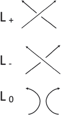
First, we must develop a version of grid homology for links, which we modify from [Reference Ozsváth, Stipcisz and Szabó5, Definition 8.2.4].
Definition 6.1 Let $\mathbb {G}$
be a grid diagram representing an
$\mathbb {G}$
be a grid diagram representing an $\ell $
-component link, and suppose
$\ell $
-component link, and suppose $O_{j_1}, \dots , O_{j_{\ell }}$
are O-markings lying on each component of the link. Then, the collapsed grid complex of
$O_{j_1}, \dots , O_{j_{\ell }}$
are O-markings lying on each component of the link. Then, the collapsed grid complex of $\mathbb {G}$
is the complex
$\mathbb {G}$
is the complex
 $$ \begin{align*}cGC_S^-(\mathbb{G}; \mathbb{Z}) := GC_S^-(\mathbb{G}; \mathbb{Z})/(V_{j_1}=\dots=V_{j_{\ell}}),\end{align*} $$
with the same differential. The homology of this complex is known as $cGH_S^-(\mathbb {G}; \mathbb {Z}).$
The collapsed double-point enhanced grid complex of $\mathbb {G}$
is the complex
$\mathbb {G}$
is the complex
 $$ \begin{align*}c\mathit{GCL}^-_S(\mathbb{G}; \mathbb{Z}) := \mathit{GCL}^-_S(\mathbb{G}; \mathbb{Z})/(V_{j_1}=\dots=V_{j_{\ell}}),\end{align*} $$
with the same differential. The homology of this complex is known as $c\mathit {GHL}^-_S(\mathbb {G}; \mathbb {Z}).$
The proof of the signed version of [Reference Ozsváth, Stipcisz and Szabó5, Theorem 8.2.5] adapts without variation to the double-point enhanced case to give the following theorem:
Theorem 6.2 For any link, the collapsed double-point enhanced grid complex of a grid diagram representing the link is a link invariant as a bigraded $\mathbb {Z}[U, v]$
-module.
$\mathbb {Z}[U, v]$
-module.
Now, we are ready to state the theorem we wish to prove. We omit the $\mathbb {Z}$
and S from the notation for convenience. Let
$\mathbb {Z}$
and S from the notation for convenience. Let $c\mathit {GHL}^-_m(L, a)$
be the
$c\mathit {GHL}^-_m(L, a)$
be the $\mathbb {Z}$
-submodule of
$\mathbb {Z}$
-submodule of $c\mathit {GHL}^-(L)$
consisting of homogenous elements of bidegree
$c\mathit {GHL}^-(L)$
consisting of homogenous elements of bidegree $(m,a).$
Theorem 6.3 Let $(L_+, L_-, L_0)$
be an oriented skein triple, with
$(L_+, L_-, L_0)$
be an oriented skein triple, with $\ell $
and
$\ell $
and $\ell _0$
the number of components of
$\ell _0$
the number of components of $L_+$
and
$L_+$
and $L_0$
, respectively. If
$L_0$
, respectively. If $\ell _0=\ell +1,$
then there is a long exact sequence where the maps below fit together to be homomorphisms of
$\ell _0=\ell +1,$
then there is a long exact sequence where the maps below fit together to be homomorphisms of $\mathbb {Z}[U, v]$
-modules:
$\mathbb {Z}[U, v]$
-modules:
 $$ \begin{align*}\to c\mathit{GHL}^-_m(L_+, s) \to c\mathit{GHL}^-_m(L_-, s) \to c\mathit{GHL}^-_{m-1}(L_0, s) \to c\mathit{GHL}^-_{m-1}(L_+, s) \to \end{align*} $$
Let J be the four-dimensional bigraded abelian group $J\cong \mathbb {Z}^4$
with one generator in bigrading
$J\cong \mathbb {Z}^4$
with one generator in bigrading $(0,1),$
one generator in bigrading
$(0,1),$
one generator in bigrading $(-2, -1),$
and two generators in bigrading
$(-2, -1),$
and two generators in bigrading $(-1, 0).$
If $\ell _0=\ell -1,$
then there is a long exact sequence where the maps below fit together to be homomorphisms of
$\ell _0=\ell -1,$
then there is a long exact sequence where the maps below fit together to be homomorphisms of $\mathbb {Z}[U, v]$
-modules:
$\mathbb {Z}[U, v]$
-modules:
 $$ \begin{align*}\to c\mathit{GHL}^-_m(L_+, s) \to c\mathit{GHL}^-_m(L_-, s) \to c\mathit{GHL}^-_{m-1}(L_0, s)\otimes J \to c\mathit{GHL}^-_{m-1}(L_+, s) \to \end{align*} $$
6.2 Proof of the theorem
Per [Reference Ozsváth, Stipcisz and Szabó5, Chapter 9], we may assume that $L_+, L_-,$
and
$L_+, L_-,$
and $L_0$
are represented by grid diagrams
$L_0$
are represented by grid diagrams $\mathbb {G}_+, \mathbb {G}_-,$
and
$\mathbb {G}_+, \mathbb {G}_-,$
and $\mathbb {G}_0,$
respectively, which we picture below along with another diagram
$\mathbb {G}_0,$
respectively, which we picture below along with another diagram $\mathbb {G}_0^{\prime }$
also representing
$\mathbb {G}_0^{\prime }$
also representing $L_0.$
The below diagram is similar to [Reference Ozsváth, Stipcisz and Szabó5, p. 153], and it depicts, left to right,
$L_0.$
The below diagram is similar to [Reference Ozsváth, Stipcisz and Szabó5, p. 153], and it depicts, left to right, $\mathbb {G}_+, \mathbb {G}_0, \mathbb {G}_0^{\prime },$
and
$\mathbb {G}_+, \mathbb {G}_0, \mathbb {G}_0^{\prime },$
and $\mathbb {G}_-.$
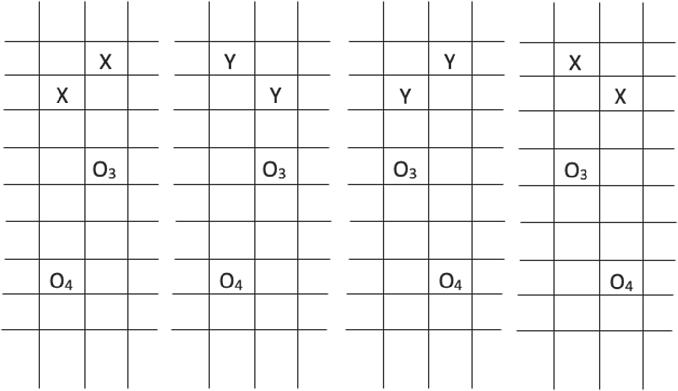
Below, we draw another diagram similar to [Reference Ozsváth, Stipcisz and Szabó5, Figure 9.3], which depicts all four of these grid diagrams simultaneously, and defines for us two crucial points c and $c'.$
Here, the solid bent line is a
$c'.$
Here, the solid bent line is a $\beta $
curve while the dashed bent line is the corresponding
$\beta $
curve while the dashed bent line is the corresponding $\gamma $
curve.
$\gamma $
curve.
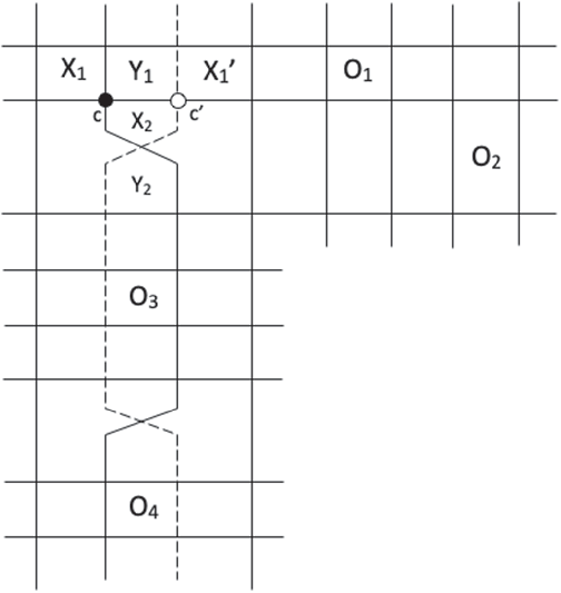
We partition our four chain complexes, as above, into $\mathbf {I}$
and
$\mathbf {I}$
and $\mathbf {N}$
parts depending on whether the grid states contain the marked point
$\mathbf {N}$
parts depending on whether the grid states contain the marked point $c,$
and
$c,$
and $\mathbf {I'}$
and
$\mathbf {I'}$
and $\mathbf {N'}$
parts depending on whether the grid states contain the marked point
$\mathbf {N'}$
parts depending on whether the grid states contain the marked point $c',$
giving the following descriptions of
$c',$
giving the following descriptions of $\mathit {GCL}^-_S$
as mapping cones of the following maps counting some of the distinguished squares in the above diagram. (We omit the
$\mathit {GCL}^-_S$
as mapping cones of the following maps counting some of the distinguished squares in the above diagram. (We omit the $\mathbb {Z}$
for notational simplicity.)
$\mathbb {Z}$
for notational simplicity.)
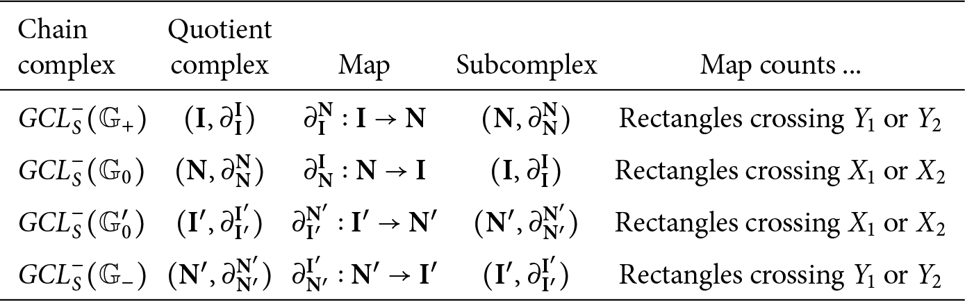
Definition 6.4 We define the map $T:\mathbf {I}^{\prime }(\mathbb {G}_0^{\prime })\rightarrow \mathbf {I}(\mathbb {G}_+)$
by the property that
$T:\mathbf {I}^{\prime }(\mathbb {G}_0^{\prime })\rightarrow \mathbf {I}(\mathbb {G}_+)$
by the property that $T(\mathbf {x}) - (T(\mathbf {x})\cap \beta _i) = \mathbf {x} - (\mathbf {x}\cap \gamma _i)$
(see [Reference Ozsváth, Stipcisz and Szabó5, p. 155]).
$T(\mathbf {x}) - (T(\mathbf {x})\cap \beta _i) = \mathbf {x} - (\mathbf {x}\cap \gamma _i)$
(see [Reference Ozsváth, Stipcisz and Szabó5, p. 155]).
Lemma 6.5 The identification $T:\mathbf {I}'(\mathbb {G}_0^{\prime })\rightarrow \mathbf {I}(\mathbb {G}_0)$
extends to an isomorphism of chain complexes over
$T:\mathbf {I}'(\mathbb {G}_0^{\prime })\rightarrow \mathbf {I}(\mathbb {G}_0)$
extends to an isomorphism of chain complexes over $\mathbb {F}[v, V_1, \dots , V_n].$
Proof The proof of [Reference Ozsváth, Stipcisz and Szabó5, Lemma 9.2.3] holds in our situation.
Lemma 6.6 The maps $\partial ^{\mathbf {I}^{\prime }}_{\mathbf {N}^{\prime }}\circ \partial ^{\mathbf {N}^{\prime }}_{\mathbf {I}^{\prime }}:\mathbf {I}^{\prime }\rightarrow \mathbf {I}^{\prime }$
and
$\partial ^{\mathbf {I}^{\prime }}_{\mathbf {N}^{\prime }}\circ \partial ^{\mathbf {N}^{\prime }}_{\mathbf {I}^{\prime }}:\mathbf {I}^{\prime }\rightarrow \mathbf {I}^{\prime }$
and $\partial ^{\mathbf {I}^{}}_{\mathbf {N}^{}}\circ \partial ^{\mathbf {N}^{}}_{\mathbf {I}^{}}:\mathbf {I}\rightarrow \mathbf {I}$
are both equal to multiplication by
$\partial ^{\mathbf {I}^{}}_{\mathbf {N}^{}}\circ \partial ^{\mathbf {N}^{}}_{\mathbf {I}^{}}:\mathbf {I}\rightarrow \mathbf {I}$
are both equal to multiplication by $V_1+V_2-V_3-V_4.$
Proof We do $\partial ^{\mathbf {I}}_{\mathbf {N}}\circ \partial ^{\mathbf {N}}_{\mathbf {I}}:\mathbf {I}\rightarrow \mathbf {I}$
first.
$\partial ^{\mathbf {I}}_{\mathbf {N}}\circ \partial ^{\mathbf {N}}_{\mathbf {I}}:\mathbf {I}\rightarrow \mathbf {I}$
first.
As in the proof of [Reference Ozsváth, Stipcisz and Szabó5, Lemma 9.2.4], we proceed by a now-familiar rectangle counting argument. Consider any juxtaposition of rectangles contributing to the left-hand side of the equation
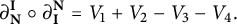 $$ \begin{align*}\partial^{\mathbf{I}^{}}_{\mathbf{N}^{}}\circ\partial^{\mathbf{N}^{}}_{\mathbf{I}^{}} = V_1+V_2-V_3-V_4. \end{align*} $$
This is a rectangle from $\mathbf {x}\in \mathbf {I}(\mathbb {G}_+)$
to
$\mathbf {x}\in \mathbf {I}(\mathbb {G}_+)$
to $\mathbf {y}\in \mathbf {N}(\mathbb {G}_+)$
(where we count rectangles going through Y markings) and then a rectangle from
$\mathbf {y}\in \mathbf {N}(\mathbb {G}_+)$
(where we count rectangles going through Y markings) and then a rectangle from $\mathbf {y}\in \mathbf {N}(\mathbb {G}_+)$
to
$\mathbf {y}\in \mathbf {N}(\mathbb {G}_+)$
to $\mathbf {z}\in \mathbf {I}(\mathbb {G}_+)$
(where we count rectangles going through X markings). Thus,
$\mathbf {z}\in \mathbf {I}(\mathbb {G}_+)$
(where we count rectangles going through X markings). Thus, $\mathbf {y}$
must not contain
$\mathbf {y}$
must not contain $c,$
but
$c,$
but $\mathbf {z}$
does. The only possibility is thus that
$\mathbf {z}$
does. The only possibility is thus that $\mathbf {x} = \mathbf {z},$
and the composite of these two rectangles must be an annulus. The annulus must be width one since otherwise it would intersect
$\mathbf {x} = \mathbf {z},$
and the composite of these two rectangles must be an annulus. The annulus must be width one since otherwise it would intersect $\mathbb {X}-\{X_1, X_2, Y_1, Y_2\},$
and similarly must be multiplicity 1.
$\mathbb {X}-\{X_1, X_2, Y_1, Y_2\},$
and similarly must be multiplicity 1.
There are four annuli, and since they are all thin, they are empty; the O-markings they pass through are $O_i$
for
$O_i$
for $i=1,2,3,4,$
giving
$i=1,2,3,4,$
giving $V_1+V_2-V_3-V_4$
since the
$V_1+V_2-V_3-V_4$
since the $V_3$
and
$V_3$
and $V_4$
terms correspond to vertical annuli whereas the others correspond to horizontal annuli.
$V_4$
terms correspond to vertical annuli whereas the others correspond to horizontal annuli.
The other case uses the same decomposition of rectangles.
We get the following commutative square:
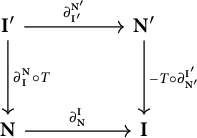
Lemma 6.7 (Modified from [Reference Ozsváth, Stipcisz and Szabó5, Lemma 9.2.5]). Let $M_0, A_0$
be the bigradings on
$M_0, A_0$
be the bigradings on $\mathbb {G}_0$
(whose grid states may be naturally identified with those of
$\mathbb {G}_0$
(whose grid states may be naturally identified with those of $\mathbb {G}_+$
) and
$\mathbb {G}_+$
) and $M_0,' A_0^{\prime }$
be the bigradings on
$M_0,' A_0^{\prime }$
be the bigradings on $\mathbb {G}_0^{\prime }$
(whose grid states may be naturally identified with those of
$\mathbb {G}_0^{\prime }$
(whose grid states may be naturally identified with those of $\mathbb {G}_-$
). Endow
$\mathbb {G}_-$
). Endow $\mathbf {I}'$
and
$\mathbf {I}'$
and $\mathbf {N}'$
with bigradings
$\mathbf {N}'$
with bigradings $M_0^{\prime }$
and
$M_0^{\prime }$
and $A_0^{\prime }+\frac {\ell _0-\ell -1}{2}$
and endow
$A_0^{\prime }+\frac {\ell _0-\ell -1}{2}$
and endow $\mathbf {I}$
and
$\mathbf {I}$
and $\mathbf {N}$
with bigradings
$\mathbf {N}$
with bigradings $M_0+1$
and
$M_0+1$
and $A_0+\frac {\ell _0-\ell +1}{2}.$
Then, in the above square, the following holds:
-
• Each edge map is homogenous of bidegree
$(-1, 0).$
-
• The left column is isomorphic as a bigraded chain complex over
$\mathbb {F}[V_1,\dots , V_n, v]$
to
$\mathit {GCL}^-_S(\mathbb {G}_+)[[-1, 0]].$
-
• The left column is isomorphic as a bigraded chain complex over
$\mathbb {F}[V_1,\dots , V_n, v]$
to
$\mathit {GCL}^-_S(\mathbb {G}_-).$
-
• The top row is isomorphic as a bigraded chain complex over
$\mathbb {F}[V_1,\dots , V_n, v]$
to
$\mathit {GCL}^-_S(\mathbb {G}_0^{\prime })[[0,\frac {\ell _0-\ell +1}{2}]].$
-
• The bottom row is isomorphic as a bigraded chain complex over
$\mathbb {F}[V_1,\dots , V_n, v]$
to
$\mathit {GCL}^-_S(\mathbb {G}_0)[[-1,\frac {\ell _0-\ell -1}{2}]].$


Proof The proofs of [Reference Ozsváth, Stipcisz and Szabó5, Lemma 9.2.3] and [Reference Ozsváth, Stipcisz and Szabó5, Lemma 9.2.5] carry over identically in this situation.
The following corollary is immediate.
Corollary 6.8 The map
 $$ \begin{align*}(-1)^M(\partial^{\mathbf{N}^{}}_{\mathbf{I}^{}}\circ T-T\circ\partial^{\mathbf{I}^{\prime}}_{\mathbf{N}^{\prime}}):\mathit{GCL}^-_S(\mathbb{G}_0^{\prime})\rightarrow \mathit{GCL}^-_S(\mathbb{G}_0)\end{align*} $$
is a chain map of $\mathbb {F}[v, V_1, \dots , V_n]$
-modules homogeneous of degree
$\mathbb {F}[v, V_1, \dots , V_n]$
-modules homogeneous of degree $(-2, -1).$
Note that the mapping cone of this map is precisely the above commutative square.
6.3 Defining the new maps
Define for $\mathbf {x} \in \mathbf {S}(\mathbb {G}_0),$
the map:
$\mathbf {x} \in \mathbf {S}(\mathbb {G}_0),$
the map:
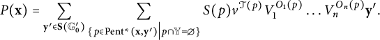 $$ \begin{align*}P(\mathbf{x}) = \sum_{\mathbf{y}'\in\mathbf{S}(\mathbb{G}_0^{\prime})}\sum_{\{p\in\operatorname{\mathrm{Pent}}^{*}(\mathbf{x}, \mathbf{y}') \big| p\cap\mathbb{Y} = \emptyset \}} S(p)v^{\mathcal{T}(p)} V_1^{O_1(p)}\dots V_n^{O_n(p)} \mathbf{y}'.\end{align*} $$
And, for $i=1,2,$
and
$i=1,2,$
and $\mathbf {x} \in \mathbf {S}(\mathbb {G}_0^{\prime }),$
the maps:
$\mathbf {x} \in \mathbf {S}(\mathbb {G}_0^{\prime }),$
the maps:
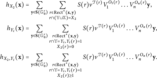 $$ \begin{align*} h_{X_2}(\mathbf{x}) &= \sum_{\mathbf{y}\in\mathbf{S}(\mathbb{G}_0^{\prime})}\sum_{\substack{r\in\operatorname{\mathrm{Rect}}^{*}(\mathbf{x}, \mathbf{y}) \\ r\cap(\mathbb{Y}\cup\mathbb{X}) = X_2\\}} S(r)v^{\mathcal{T}(r)} V_1^{O_1(r)}\dots V_n^{O_n(r)} \mathbf{y}, \\ h_{Y_i}(\mathbf{x}) &= \sum_{\mathbf{y}\in\mathbf{S}(\mathbb{G}_0^{\prime})}\sum_{\substack{r\in\operatorname{\mathrm{Rect}}^{*}(\mathbf{x}, \mathbf{y}) \\ r\cap\mathbb{Y} = Y_i, Y_i(r)=1 \\ X_2(r)=0\\}} S(r)v^{\mathcal{T}(r)} V_1^{O_1(r)}\dots V_n^{O_n(r)} \mathbf{y}, \\ h_{X_2, Y_i}(\mathbf{x}) &= \sum_{\mathbf{y}\in\mathbf{S}(\mathbb{G}_0^{\prime})}\sum_{\substack{r\in\operatorname{\mathrm{Rect}}^{*}(\mathbf{x}, \mathbf{y}) \\ r\cap\mathbb{Y} = Y_i, Y_i(r)=1 \\ X_2(r)\geq1\\}} S(r)v^{\mathcal{T}(r)} V_1^{O_1(r)}\dots V_n^{O_n(r)} \mathbf{y}. \end{align*} $$
Let $h_Y = h_{Y_1} + h_{Y_2}$
and
$h_Y = h_{Y_1} + h_{Y_2}$
and $h_{X_2, Y} = h_{X_2, Y_1} + h_{X_2, Y_2}$
.
$h_{X_2, Y} = h_{X_2, Y_1} + h_{X_2, Y_2}$
.
Further define, for a domain $\psi ,$
the quantity
$\psi ,$
the quantity $Y(\psi ) = Y_1(\psi )+Y_2(\psi ).$
Lemma 6.9 The map $P:\mathit {GCL}^-_S(\mathbb {G}_0)\rightarrow \mathit {GCL}^-_S(\mathbb {G}_0^{\prime })$
is a quasi-isomorphism of bigraded chain complexes.
$P:\mathit {GCL}^-_S(\mathbb {G}_0)\rightarrow \mathit {GCL}^-_S(\mathbb {G}_0^{\prime })$
is a quasi-isomorphism of bigraded chain complexes.
Proof This is immediate from the commutation invariance of $\mathit {GCL}^-_S$
as proven in the previous section. Alternatively, the unsigned version of this lemma is proven in [Reference Ratigan, Wang and Wang9, Propositions 9–11]. (This paper uses a slightly different-looking definition for the map P, allowing pentagons to be long without being thin, however, these pentagons always contribute 0 since they contain intersections with
$\mathit {GCL}^-_S$
as proven in the previous section. Alternatively, the unsigned version of this lemma is proven in [Reference Ratigan, Wang and Wang9, Propositions 9–11]. (This paper uses a slightly different-looking definition for the map P, allowing pentagons to be long without being thin, however, these pentagons always contribute 0 since they contain intersections with $\mathbb {X},$
hence the two maps are in fact identical.)
$\mathbb {X},$
hence the two maps are in fact identical.)
Remark 6.10 $h_{X_2, Y_i}$
does not vanish on
$h_{X_2, Y_i}$
does not vanish on $\mathbf {I}^{\prime }.$
This is in stark contrast to the map
$\mathbf {I}^{\prime }.$
This is in stark contrast to the map $h_{X_2, Y_i}$
defined in [Reference Ozsváth, Stipcisz and Szabó5, Chapter 9] in the un-enhanced case.
$h_{X_2, Y_i}$
defined in [Reference Ozsváth, Stipcisz and Szabó5, Chapter 9] in the un-enhanced case.
Lemma 6.11
-
(1)
$h_{X_2}$
vanishes on
$\mathbf {N}^{\prime }$
and maps
$\mathbf {I}^{\prime }$
to
$\mathbf {N}^{\prime }$
. -
(2)
$h_{Y}$
vanishes on
$\mathbf {I}^{\prime }$
.


Proof Both statements follow immediately from the multiplicity conditions on the rectangles in the definitions of the maps.
Lemma 6.12
-
(1) Suppose r is a rectangle contributing to the sum in
$h_{X_2}$
. Then r is not long, and
$Y_1(r)=Y_2(r)=0.$
-
(2) Suppose
$r\in \operatorname {\mathrm {Rect}}^{*}(\mathbf {x}, \mathbf {y})$
is a rectangle contributing to the sum in
$h_{X_2, Y_i}.$
Then,
$\mathbf {y}\in \mathbf {N}(\mathbb {G}_0^{\prime }),$
so as a consequence, the image of
$h_{X_2, Y_i}$
is within
$\mathbf {N}^{\prime }.$


Proof Both statements follow immediately from the multiplicity conditions on the $Y_i$
in the definitions of the maps.
$Y_i$
in the definitions of the maps.
Now, we must prove two key lemmas.
Lemma 6.13 The following two identities hold:
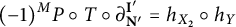 $$ \begin{align*}(-1)^MP\circ T\circ \partial^{\mathbf{I}^{\prime}}_{\mathbf{N}^{\prime}} = h_{X_2}\circ h_Y\end{align*} $$
and
 $$ \begin{align*}(-1)^{M+1}P\circ \partial^{\mathbf{N}^{}}_{\mathbf{I}^{}}\circ T = h_{Y}\circ h_{X_2}.\end{align*} $$
Proof We start with the first equation. Let $\psi = r*t*p$
be a domain contributing to the left-hand side. Here, since the image of T is in
$\psi = r*t*p$
be a domain contributing to the left-hand side. Here, since the image of T is in $\mathbf {I}^{\prime },$
a pentagon p contributing to P in the left-hand side has an outgoing corner at
$\mathbf {I}^{\prime },$
a pentagon p contributing to P in the left-hand side has an outgoing corner at $c,$
therefore geometrically we see
$c,$
therefore geometrically we see $X_2(p)=0$
lest
$X_2(p)=0$
lest $Y_i(p)\geq 0$
for either
$Y_i(p)\geq 0$
for either $i=1,2.$
Now, concatenating p with the triangle t contributing to t, therefore gives a rectangle
$i=1,2.$
Now, concatenating p with the triangle t contributing to t, therefore gives a rectangle $r_2$
with an outgoing corner at
$r_2$
with an outgoing corner at $c',$
with
$c',$
with $X_2(r_2)=1,$
and
$X_2(r_2)=1,$
and $Y_1(r_2)=Y_2(r_2)=0.$
Furthermore, the image of
$Y_1(r_2)=Y_2(r_2)=0.$
Furthermore, the image of $\partial ^{\mathbf {I}^{\prime }}_{\mathbf {N}^{\prime }}$
is some rectangle
$\partial ^{\mathbf {I}^{\prime }}_{\mathbf {N}^{\prime }}$
is some rectangle $r=r_1$
with an incoming corner at
$r=r_1$
with an incoming corner at $c'$
, and with
$c'$
, and with $Y(r_1) = 1.$
Hence, the composite
$Y(r_1) = 1.$
Hence, the composite $\psi = r_1*r_2$
is a decomposition appearing in the right-hand side. Conversely, for
$\psi = r_1*r_2$
is a decomposition appearing in the right-hand side. Conversely, for $\psi = r_1*r_2$
, a decomposition appearing in the right-hand side, we have that the rectangle
$\psi = r_1*r_2$
, a decomposition appearing in the right-hand side, we have that the rectangle $r_1=r$
contributes to
$r_1=r$
contributes to $ \partial ^{\mathbf {I}^{\prime }}_{\mathbf {N}^{\prime }},$
and cutting
$ \partial ^{\mathbf {I}^{\prime }}_{\mathbf {N}^{\prime }},$
and cutting $r_2$
along the portion of
$r_2$
along the portion of $\beta _i$
passing through
$\beta _i$
passing through $X_2$
gives us a decomposition
$X_2$
gives us a decomposition $r_2 = t*p$
such that t contributes to T and p to P in the left-hand side. Furthermore, these two decompositions always have the same degree since the interiors of the domains in each decomposition differ only on the edge of the small triangle t which is part of
$r_2 = t*p$
such that t contributes to T and p to P in the left-hand side. Furthermore, these two decompositions always have the same degree since the interiors of the domains in each decomposition differ only on the edge of the small triangle t which is part of $\beta _i$
; however, the only point on
$\beta _i$
; however, the only point on $\beta _i$
that could possibly affect the degrees of the decompositions is an outgoing corner of
$\beta _i$
that could possibly affect the degrees of the decompositions is an outgoing corner of $p.$
Hence, either
$p.$
Hence, either $\mathcal {T}(p)=\mathcal {T}(r_2)=1$
or else
$\mathcal {T}(p)=\mathcal {T}(r_2)=1$
or else $\mathcal {T}(p)=\mathcal {T}(r_2)=0$
. Furthermore, by the definition of a sign assignment for a pentagon, it is clear that both decompositions have the same sign.
$\mathcal {T}(p)=\mathcal {T}(r_2)=0$
. Furthermore, by the definition of a sign assignment for a pentagon, it is clear that both decompositions have the same sign.
Now, we consider the second equation. Let $\psi = t*r*p$
be a domain contributing to the left-hand side. We see geometrically that if
$\psi = t*r*p$
be a domain contributing to the left-hand side. We see geometrically that if $X_2(p)\geq 1,$
then it must be the case that either
$X_2(p)\geq 1,$
then it must be the case that either $Y_1(p)$
or
$Y_1(p)$
or $Y_2(p)$
is positive. Since we specify in the equation defining P that
$Y_2(p)$
is positive. Since we specify in the equation defining P that $Y(p)=0,$
we must have
$Y(p)=0,$
we must have $X_2(p)=0.$
Furthermore, it is not possible for r and p to overlap in a small neighborhood of
$X_2(p)=0.$
Furthermore, it is not possible for r and p to overlap in a small neighborhood of $c',$
since this would require
$c',$
since this would require $Y_1(r)=1$
and then
$Y_1(r)=1$
and then $Y(p)>0.$
Hence, all local multiplicities are
$Y(p)>0.$
Hence, all local multiplicities are $\leq 1$
around
$\leq 1$
around $c'.$
Suppose
$c'.$
Suppose $c'$
were a 90-degree corner. Then, we must have
$c'$
were a 90-degree corner. Then, we must have $Y_2(r)=1,$
and p must be a left pentagon. However, geometrically, the only way this is possible is if
$Y_2(r)=1,$
and p must be a left pentagon. However, geometrically, the only way this is possible is if $Y_2(p)\geq 1,$
a contradiction.
$Y_2(p)\geq 1,$
a contradiction.
Also note that $X_2(r) = 0$
by the fact that c is an outgoing corner and r cannot be long. In all cases, then, we have
$X_2(r) = 0$
by the fact that c is an outgoing corner and r cannot be long. In all cases, then, we have $X_2(\psi ) = Y(\psi ) = 1.$
Thus, $c'$
is either a 270-degree corner, a 180-degree corner, or in the interior of
$c'$
is either a 270-degree corner, a 180-degree corner, or in the interior of $\psi $
. In all three cases, we may represent
$\psi $
. In all three cases, we may represent $\psi $
by an L-shaped region Q in the universal cover such that a pre-image
$\psi $
by an L-shaped region Q in the universal cover such that a pre-image $C'$
of
$C'$
of $c'$
is either a 270-degree corner, a 180-degree corner, or in the interior of
$c'$
is either a 270-degree corner, a 180-degree corner, or in the interior of $\psi $
. Indeed, start with t which has a corner at
$\psi $
. Indeed, start with t which has a corner at $C',$
and then attach pre-images R and P of r and p such that if r or p has a corner at
$C',$
and then attach pre-images R and P of r and p such that if r or p has a corner at $c'$
, then R or P has a corner at
$c'$
, then R or P has a corner at $C'.$
$C'.$
We must also show that these three possibilities are also the only three possibilities for a domain contributing to the right-hand side. Suppose $\psi = r_1*r_2$
, where
$\psi = r_1*r_2$
, where $r_1$
is from
$r_1$
is from $h_{X_2}$
and
$h_{X_2}$
and $r_2$
is from
$r_2$
is from $h_Y.$
Then,
$h_Y.$
Then, $r_1$
has a corner at
$r_1$
has a corner at $c',$
namely the southwest corner, and no others since
$c',$
namely the southwest corner, and no others since $Y(r_1)=0.$
Then,
$Y(r_1)=0.$
Then, $r_2$
must contain precisely one of
$r_2$
must contain precisely one of $Y_1$
or
$Y_1$
or $Y_2,$
but
$Y_2,$
but $X_2(r_2)=0,$
so either
$X_2(r_2)=0,$
so either $r_2$
has a corner at
$r_2$
has a corner at $c',$
leaving
$c',$
leaving $\psi $
a 180-degree corner at
$\psi $
a 180-degree corner at $c'$
(which clearly forces
$c'$
(which clearly forces $\psi $
to be an annulus), or it has an edge passing through
$\psi $
to be an annulus), or it has an edge passing through $c',$
leaving
$c',$
leaving $\psi $
a 270-degree corner at
$\psi $
a 270-degree corner at $c'.$
Note that there is no 360-degree case; we will return to this at the end of the proof.
$c'.$
Note that there is no 360-degree case; we will return to this at the end of the proof.
We will first show that in each case $\psi $
has two decompositions of equal degree; then, we will appeal to a proof from [Reference Ozsváth, Stipcisz and Szabó5] to show that these two decompositions further have the same sign.
$\psi $
has two decompositions of equal degree; then, we will appeal to a proof from [Reference Ozsváth, Stipcisz and Szabó5] to show that these two decompositions further have the same sign.
In the first 270-degree case, either $c'$
is on an edge of r or on
$c'$
is on an edge of r or on $p.$
If
$p.$
If $c'$
is on an edge of
$c'$
is on an edge of $r,$
which is part of horizontal circle, say,
$r,$
which is part of horizontal circle, say, $\alpha _j,$
then cutting
$\alpha _j,$
then cutting $\psi $
along
$\psi $
along $\alpha _j$
gives a decomposition
$\alpha _j$
gives a decomposition $\psi = r_1*r_2.$
Since
$\psi = r_1*r_2.$
Since $r_1$
clearly has c as an outgoing corner and contains
$r_1$
clearly has c as an outgoing corner and contains $X_2,$
and we know
$X_2,$
and we know $X_2(\psi )=X_2(r)+X_2(t)+X_2(p)=0+1+0=1,$
that tells us
$X_2(\psi )=X_2(r)+X_2(t)+X_2(p)=0+1+0=1,$
that tells us $X_2(r_1)=1.$
Furthermore, in this case, the support of
$X_2(r_1)=1.$
Furthermore, in this case, the support of $r_1$
is a subset of the support of
$r_1$
is a subset of the support of $p,$
hence
$p,$
hence $Y(r_1)=0.$
Thus,
$Y(r_1)=0.$
Thus, $r_1$
contributes to
$r_1$
contributes to $h_{X_2}$
; likewise, we must have
$h_{X_2}$
; likewise, we must have $Y(r_2)=Y(\psi )=1,$
so Y contributes to
$Y(r_2)=Y(\psi )=1,$
so Y contributes to $h_Y.$
Conversely, if
$h_Y.$
Conversely, if $\psi = r_1*r_2,$
with
$\psi = r_1*r_2,$
with $Y_1(r_2)=1,$
then performing this same cut along
$Y_1(r_2)=1,$
then performing this same cut along $\alpha _j$
gives a decomposition as in the left-hand side.
$\alpha _j$
gives a decomposition as in the left-hand side.
The proof of Lemma 4.3 ensures that the two decompositions $r_1*r_2$
and
$r_1*r_2$
and $r_1^{\prime }*r_2^{\prime }$
of
$r_1^{\prime }*r_2^{\prime }$
of $\psi $
as rectangles in
$\psi $
as rectangles in $\mathit {GCL}^-(\mathbb {G}_0^{\prime })$
have the same degree. One of these decompositions is
$\mathit {GCL}^-(\mathbb {G}_0^{\prime })$
have the same degree. One of these decompositions is $r_1*r_2,$
and the other
$r_1*r_2,$
and the other $p*r*t$
differs from
$p*r*t$
differs from $r_1^{\prime }*r_2^{\prime }$
by the introduction of the small triangle t and by cutting at
$r_1^{\prime }*r_2^{\prime }$
by the introduction of the small triangle t and by cutting at $\beta _i$
instead of
$\beta _i$
instead of $\gamma _i$
. No points on
$\gamma _i$
. No points on $\beta _i$
or
$\beta _i$
or $\gamma _i$
can contribute to the degrees of any of these decompositions, for on the left-hand side, p and r border
$\gamma _i$
can contribute to the degrees of any of these decompositions, for on the left-hand side, p and r border $\beta _i$
and on the right-hand side,
$\beta _i$
and on the right-hand side, $r_1$
and
$r_1$
and $r_2$
border
$r_2$
border $\gamma _i.$
Thus, both decompositions
$\gamma _i.$
Thus, both decompositions $r_1*r_2$
and
$r_1*r_2$
and $p*r*t$
have the same degree.
$p*r*t$
have the same degree.
Similarly, if $c'$
is on an edge of
$c'$
is on an edge of $p,$
then this edge is part of
$p,$
then this edge is part of $\gamma _i,$
and we cut
$\gamma _i,$
and we cut $\psi $
along
$\psi $
along $\gamma _i$
to get a decomposition
$\gamma _i$
to get a decomposition $r_1*r_2.$
In this case,
$r_1*r_2.$
In this case, $r_1$
is the union of t and a portion of r not containing
$r_1$
is the union of t and a portion of r not containing $Y_2$
; hence,
$Y_2$
; hence, $X_2(r_1)=1$
and
$X_2(r_1)=1$
and $Y(r_1)=0,$
so
$Y(r_1)=0,$
so $r_1$
contributes to
$r_1$
contributes to $h_{X_2}.$
Similarly,
$h_{X_2}.$
Similarly, $r_2$
must contribute to
$r_2$
must contribute to $h_Y$
since we must have
$h_Y$
since we must have $Y(r_2)=1$
. Conversely, if
$Y(r_2)=1$
. Conversely, if $\psi = r_1*r_2,$
with
$\psi = r_1*r_2,$
with $Y_2(r_2)=1,$
then performing this same cut along
$Y_2(r_2)=1,$
then performing this same cut along $\gamma _i$
gives a decomposition as in the left-hand side. Likewise, these two decompositions differ by the introduction of the small triangle t and by cutting at
$\gamma _i$
gives a decomposition as in the left-hand side. Likewise, these two decompositions differ by the introduction of the small triangle t and by cutting at $\beta _i$
instead of
$\beta _i$
instead of $\gamma _i$
, so they also must have the same degree by the argument in the previous paragraph.
$\gamma _i$
, so they also must have the same degree by the argument in the previous paragraph.
In the 180-degree case on the left-hand side, we must have $Y_2(r)=1,$
and since r is not long, the condition that there is a 180-degree corner at
$Y_2(r)=1,$
and since r is not long, the condition that there is a 180-degree corner at $c'$
forces p to have an incoming corner at
$c'$
forces p to have an incoming corner at $c',$
and also for
$c',$
and also for $\mathbf {x} = \mathbf {z}$
; hence, the region
$\mathbf {x} = \mathbf {z}$
; hence, the region $\psi $
must be a horizontal annulus, and it must be thin to avoid intersecting with
$\psi $
must be a horizontal annulus, and it must be thin to avoid intersecting with $\mathbb {Y}-\{Y_1, Y_2\}$
. Furthermore, since the local multiplicities of
$\mathbb {Y}-\{Y_1, Y_2\}$
. Furthermore, since the local multiplicities of $c',$
which is an incoming corner of
$c',$
which is an incoming corner of $p,$
are all
$p,$
are all $\leq 1,$
we must have that the annulus has multiplicity 1. There is clearly a unique decomposition of this annulus into two rectangles
$\leq 1,$
we must have that the annulus has multiplicity 1. There is clearly a unique decomposition of this annulus into two rectangles $r_1, r_2$
such that
$r_1, r_2$
such that $X_2(r_1)=Y(r_2)=1$
and
$X_2(r_1)=Y(r_2)=1$
and $Y(r_1)=X_2(r_2)=0.$
Conversely, if
$Y(r_1)=X_2(r_2)=0.$
Conversely, if $\psi = r_1*r_2$
has a 180-degree corner at
$\psi = r_1*r_2$
has a 180-degree corner at $c',$
either we are in the horizontal case, in which case there is a unique decomposition
$c',$
either we are in the horizontal case, in which case there is a unique decomposition $\psi = t*r*p$
as in the previous paragraph, or else we are in the vertical case (see the following paragraph); this case is unique for each grid state
$\psi = t*r*p$
as in the previous paragraph, or else we are in the vertical case (see the following paragraph); this case is unique for each grid state $\mathbf {x}$
. Since the annulus is thin, all constituent polygons must be empty so the degrees of all decompositions are 0.
$\mathbf {x}$
. Since the annulus is thin, all constituent polygons must be empty so the degrees of all decompositions are 0.
There is one case remaining for the left-hand side and one case remaining for the right-hand side. For the left-hand side, this case is that $c'$
is a 360-degree corner, in which case, we must have
$c'$
is a 360-degree corner, in which case, we must have $Y_1(r)=1$
and therefore that
$Y_1(r)=1$
and therefore that $c'$
is an incoming corner at p; again, this forces the initial and final grid states to be equal, so we have a vertical annulus, and it is unique for each grid state
$c'$
is an incoming corner at p; again, this forces the initial and final grid states to be equal, so we have a vertical annulus, and it is unique for each grid state $\mathbf {x}.$
The remaining case for the right-hand side is a vertical annulus as well. Both annuli are thin, so have degree 0, and contribute 1 power of
$\mathbf {x}.$
The remaining case for the right-hand side is a vertical annulus as well. Both annuli are thin, so have degree 0, and contribute 1 power of $V_4$
to the formula.
$V_4$
to the formula.
What’s left to show is that each decomposition in every case has the same sign. Since each of these possibilities is identical to those in the proof of [Reference Ozsváth, Stipcisz and Szabó5, Theorem 15.5.1], this proof guarantees that each decomposition has the same sign. Indeed, it only uses the defining properties of sign assignments and the relation between the sign of a pentagon and its associated rectangle, all of which carry over to the case where the pentagons and rectangles are potentially long.
This concludes the proof.
Lemma 6.14 The map $h_{X_2, Y}$
provides a chain homotopy from
$h_{X_2, Y}$
provides a chain homotopy from $h_{X_2}\circ h_Y + h_{Y}\circ h_{X_2}$
to multiplication by
$h_{X_2}\circ h_Y + h_{Y}\circ h_{X_2}$
to multiplication by $V_2-V_4$
, i. e. the following equation holds:
$V_2-V_4$
, i. e. the following equation holds:
 $$ \begin{align*}h_{X_2}\circ h_Y + h_{Y}\circ h_{X_2} + h_{X_2, Y}\circ \partial + \partial\circ h_{X_2, Y} = V_2 - V_4.\end{align*} $$
Proof Let $\psi \in \pi (\mathbf {x}, \mathbf {z})$
be a region contributing to the left-hand side of this equation with
$\psi \in \pi (\mathbf {x}, \mathbf {z})$
be a region contributing to the left-hand side of this equation with $\lvert D(\psi )\rvert>0.$
We have three cases,
$\lvert D(\psi )\rvert>0.$
We have three cases, $\lvert \mathbf {x} - (\mathbf {x}\cap \mathbf {z})\rvert = $
0, 3, or 4.
$\lvert \mathbf {x} - (\mathbf {x}\cap \mathbf {z})\rvert = $
0, 3, or 4.
If $\lvert \mathbf {x} - (\mathbf {x}\cap \mathbf {z})\rvert = 4,$
then Lemma 4.2 shows that
$\lvert \mathbf {x} - (\mathbf {x}\cap \mathbf {z})\rvert = 4,$
then Lemma 4.2 shows that $\lvert D(\psi )\rvert =2,$
and both decompositions have the same degree and opposite signs. Hence, this case clearly contributes 0 to the sum on the left-hand side.
$\lvert D(\psi )\rvert =2,$
and both decompositions have the same degree and opposite signs. Hence, this case clearly contributes 0 to the sum on the left-hand side.
If $\lvert \mathbf {x} - (\mathbf {x}\cap \mathbf {z})\rvert = 3,$
then Lemma 4.3 shows that
$\lvert \mathbf {x} - (\mathbf {x}\cap \mathbf {z})\rvert = 3,$
then Lemma 4.3 shows that $\lvert D(\psi )\rvert =2,$
and both decompositions have the same degree and opposite signs, since only 1 rectangle in each possible decomposition of
$\lvert D(\psi )\rvert =2,$
and both decompositions have the same degree and opposite signs, since only 1 rectangle in each possible decomposition of $\psi $
could be long. We must show that both decompositions appear in the above formula, and do so exactly once. By analyzing the above formula, we conclude that
$\psi $
could be long. We must show that both decompositions appear in the above formula, and do so exactly once. By analyzing the above formula, we conclude that $Y(\psi ) = 1$
and
$Y(\psi ) = 1$
and $X_2(\psi )\geq 1.$
Both rectangles in both decompositions clearly have trivial intersections with
$X_2(\psi )\geq 1.$
Both rectangles in both decompositions clearly have trivial intersections with $\mathbb {Y} - \{Y_1, Y_2\}$
. Hence, the only possibilities can be found by considering multiplicities of
$\mathbb {Y} - \{Y_1, Y_2\}$
. Hence, the only possibilities can be found by considering multiplicities of $X_2$
and
$X_2$
and $Y_i,$
and are listed below. Note that in the first two cases,
$Y_i,$
and are listed below. Note that in the first two cases, $r_1$
is not forced; it could be from either
$r_1$
is not forced; it could be from either $h_{X_2}$
or
$h_{X_2}$
or $\partial ,$
but this choice is forced when we consider
$\partial ,$
but this choice is forced when we consider $r_2.$
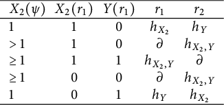
Finally, I claim the case $X_2(\psi )>1$
,
$X_2(\psi )>1$
, $X_2(r_1)=0$
, and
$X_2(r_1)=0$
, and $Y(r_1)=1$
cannot occur. Indeed, this forces the other rectangle
$Y(r_1)=1$
cannot occur. Indeed, this forces the other rectangle $r_2$
to satisfy
$r_2$
to satisfy $X_2(r_2)>1$
but also
$X_2(r_2)>1$
but also $Y(r_2)=0$
which is impossible.
$Y(r_2)=0$
which is impossible.
Hence, this case $\lvert \mathbf {x} - (\mathbf {x}\cap \mathbf {z})\rvert = 3$
also contributes 0 to the sum.
$\lvert \mathbf {x} - (\mathbf {x}\cap \mathbf {z})\rvert = 3$
also contributes 0 to the sum.
If $\lvert \mathbf {x} - (\mathbf {x}\cap \mathbf {z})\rvert = 0,$
then we must have
$\lvert \mathbf {x} - (\mathbf {x}\cap \mathbf {z})\rvert = 0,$
then we must have $\psi $
is an annulus containing
$\psi $
is an annulus containing $X_2,$
and it must be thin since
$X_2,$
and it must be thin since $Y(\psi )=1$
and
$Y(\psi )=1$
and $\psi \cap (\mathbb {Y} - \{Y_1, Y_2\}) = \emptyset .$
Since
$\psi \cap (\mathbb {Y} - \{Y_1, Y_2\}) = \emptyset .$
Since $Y(\psi )=1,$
it must have multiplicity 1. Then, clearly,
$Y(\psi )=1,$
it must have multiplicity 1. Then, clearly, $\psi $
has a unique decomposition into two rectangles, and the possibilities in the table in the previous case still apply to show that this decomposition appears precisely once in the sum on the left-hand side. If the annulus is horizontal, it gives us multiplication by
$\psi $
has a unique decomposition into two rectangles, and the possibilities in the table in the previous case still apply to show that this decomposition appears precisely once in the sum on the left-hand side. If the annulus is horizontal, it gives us multiplication by $V_2,$
and if it is vertical, we get multiplication by
$V_2,$
and if it is vertical, we get multiplication by $-V_4.$
The remainder of the proof of the skein exact sequence proceeds exactly as in [Reference Ozsváth, Stipcisz and Szabó5, Chapter 9], which gives us the theorem.
7 Alternatives to
$\tau $

In this section, we discuss constructions relating to and generalizing the $\tau $
invariant. We first recall the definition of
$\tau $
invariant. We first recall the definition of $\tau .$
Definition 7.1 For a knot K, $\tau (K)$
is
$\tau (K)$
is $-1$
times the maximum Alexander grading of a homogeneous nontorsion element in
$-1$
times the maximum Alexander grading of a homogeneous nontorsion element in $\mathit {GH}^-(K).$
Note that for the remainder of the paper, the coefficient field will be $\mathbb {F}$
unless otherwise stated. We use a field for coefficients to maximize simplicity here, although much of the below can be generalized to
$\mathbb {F}$
unless otherwise stated. We use a field for coefficients to maximize simplicity here, although much of the below can be generalized to $\mathbb {Z}$
coefficients without too much difficulty.
$\mathbb {Z}$
coefficients without too much difficulty.
7.1 The endomorphism
$\partial _1$

[Reference Lipshitz1, p. 9] briefly mentions the fact that $\partial _1$
is a chain map. Let’s recall why. The differential is defined as
$\partial _1$
is a chain map. Let’s recall why. The differential is defined as $\partial (\mathbf {x}) = \sum _{k=0}^{\infty } v^k\partial _k(\mathbf {x}).$
In proving that
$\partial (\mathbf {x}) = \sum _{k=0}^{\infty } v^k\partial _k(\mathbf {x}).$
In proving that $\partial ^2 = 0,$
we may expand out this sum and conclude that each coefficient of
$\partial ^2 = 0,$
we may expand out this sum and conclude that each coefficient of $v^k$
is 0. This gives
$v^k$
is 0. This gives
 $$ \begin{align*}\partial_0^2 = 0,\end{align*} $$
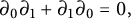 $$ \begin{align*}\partial_0\partial_1+\partial_1\partial_0 = 0,\end{align*} $$
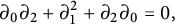 $$ \begin{align*}\partial_0\partial_2+\partial_1^2+\partial_2\partial_0 = 0,\end{align*} $$
and so on.
The second equality tells us that $\partial _1:\mathit {GC}^-(\mathbb {G})\rightarrow \mathit {GC}^-(\mathbb {G})$
is a chain map on the unblocked grid homology, so it induces a homomorphism
$\partial _1:\mathit {GC}^-(\mathbb {G})\rightarrow \mathit {GC}^-(\mathbb {G})$
is a chain map on the unblocked grid homology, so it induces a homomorphism $\partial _{1*}:\mathit {GH}^-(\mathbb {G})\rightarrow \mathit {GH}^-(\mathbb {G}).$
Furthermore, the third equation tells us that
$\partial _{1*}:\mathit {GH}^-(\mathbb {G})\rightarrow \mathit {GH}^-(\mathbb {G}).$
Furthermore, the third equation tells us that $\partial _1^2$
is nullhomotopic, hence
$\partial _1^2$
is nullhomotopic, hence $\partial _{1*}$
is a differential on
$\partial _{1*}$
is a differential on $\mathit {GH}^-(\mathbb {G})$
and we can consider its homology.
$\mathit {GH}^-(\mathbb {G})$
and we can consider its homology.
I conjecture that $\partial _{1*}$
is the zero homomorphism, but we have yet to find a nullhomotopy for it. The author has attempted to try using certain L-shaped regions as a count; this fails. However, we can show that this endomorphism is, in a certain sense, an invariant of the knot.
$\partial _{1*}$
is the zero homomorphism, but we have yet to find a nullhomotopy for it. The author has attempted to try using certain L-shaped regions as a count; this fails. However, we can show that this endomorphism is, in a certain sense, an invariant of the knot.
Theorem 7.2 Suppose that $\mathbb {G}$
and
$\mathbb {G}$
and $\mathbb {G}'$
are two grid diagrams representing the same knot and
$\mathbb {G}'$
are two grid diagrams representing the same knot and $F:\mathit {GH}^-(\mathbb {G})\to \mathit {GH}^-(\mathbb {G}')$
is an isomorphism of bigraded
$F:\mathit {GH}^-(\mathbb {G})\to \mathit {GH}^-(\mathbb {G}')$
is an isomorphism of bigraded $\mathbb {F}[U, v]$
-modules associated with a sequence of grid moves from
$\mathbb {F}[U, v]$
-modules associated with a sequence of grid moves from $\mathbb {G}$
to
$\mathbb {G}$
to $\mathbb {G}',$
as in Section 5. Then, the below diagram commutes:
$\mathbb {G}',$
as in Section 5. Then, the below diagram commutes:
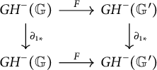
Proof By Theorem 2.10, it is sufficient to show this theorem in the case that $\mathbb {G}$
and
$\mathbb {G}$
and $\mathbb {G}'$
differ by a commutation and any type X stabilization or destabilization.
$\mathbb {G}'$
differ by a commutation and any type X stabilization or destabilization.
For the commutation maps, let $\mathbb {G}$
and
$\mathbb {G}$
and $\mathbb {G}'$
differ by a commutation or a switch. We know by our proof of invariance that there is a chain map
$\mathbb {G}'$
differ by a commutation or a switch. We know by our proof of invariance that there is a chain map $P_S:(\mathit {GCL}^-_S(\mathbb {G}), \partial )\rightarrow (\mathit {GCL}^-_S(\mathbb {G}'), \partial )$
such that the
$P_S:(\mathit {GCL}^-_S(\mathbb {G}), \partial )\rightarrow (\mathit {GCL}^-_S(\mathbb {G}'), \partial )$
such that the $v^0$
-term of
$v^0$
-term of $P_S$
, when reduced modulo 2, is precisely the quasi-isomorphism
$P_S$
, when reduced modulo 2, is precisely the quasi-isomorphism $P:(\mathit {GC}^-(\mathbb {G}), \partial _0)\rightarrow (\mathit {GC}^-(\mathbb {G}'), \partial _0)$
from [Reference Ozsváth, Stipcisz and Szabó5, Section 5.1]. Let
$P:(\mathit {GC}^-(\mathbb {G}), \partial _0)\rightarrow (\mathit {GC}^-(\mathbb {G}'), \partial _0)$
from [Reference Ozsváth, Stipcisz and Szabó5, Section 5.1]. Let $P_L$
be the reduction of
$P_L$
be the reduction of $P_S$
modulo 2. Let
$P_S$
modulo 2. Let $P_1$
be the
$P_1$
be the $v^1$
term of
$v^1$
term of $P_L.$
Then, the
$P_L.$
Then, the $v^1$
-term of the equation
$v^1$
-term of the equation
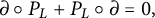 $$ \begin{align*}\partial\circ P_L + P_L\circ\partial = 0,\end{align*} $$
which expresses that $P_L$
is a chain map, is
$P_L$
is a chain map, is
 $$ \begin{align*}\partial_0\circ P_1 + P_1\circ\partial_0+\partial_1\circ P + P\circ\partial_1 = 0,\end{align*} $$
which tells us that $\partial _1$
commutes with P up to homotopy. Hence,
$\partial _1$
commutes with P up to homotopy. Hence, $\partial _{1*}$
is preserved under commutation.
$\partial _{1*}$
is preserved under commutation.
For SW-destabilization, if $\mathbb {G}'$
differs from
$\mathbb {G}'$
differs from $\mathbb {G}$
by a SW-destabilization, [Reference Ozsváth, Stipcisz and Szabó5, Lemma 5.2.17] gives us a quasi-isomorphism from
$\mathbb {G}$
by a SW-destabilization, [Reference Ozsváth, Stipcisz and Szabó5, Lemma 5.2.17] gives us a quasi-isomorphism from $\mathit {GC}^-(\mathbb {G})$
to the mapping cone of the function
$\mathit {GC}^-(\mathbb {G})$
to the mapping cone of the function $V_2-V_1:\mathit {GC}^-(\mathbb {G}')[V_1][[1,1]]\rightarrow \mathit {GC}^-(\mathbb {G}')[V_1].$
Using notation from [Reference Ozsváth, Stipcisz and Szabó5, Section 5.2], the quasi-isomorphism is given by
$V_2-V_1:\mathit {GC}^-(\mathbb {G}')[V_1][[1,1]]\rightarrow \mathit {GC}^-(\mathbb {G}')[V_1].$
Using notation from [Reference Ozsváth, Stipcisz and Szabó5, Section 5.2], the quasi-isomorphism is given by $(i,n)\mapsto (e(i), e(\mathcal {H}_{X_2}^{\mathbf {I}}(n))),$
for
$(i,n)\mapsto (e(i), e(\mathcal {H}_{X_2}^{\mathbf {I}}(n))),$
for $(i, n)\in \mathbf {I}\oplus \mathbf {N}$
. The map e clearly commutes with
$(i, n)\in \mathbf {I}\oplus \mathbf {N}$
. The map e clearly commutes with $\partial _1,$
and the map
$\partial _1,$
and the map $\partial _1$
commutes with
$\partial _1$
commutes with $\mathcal {H}_{X_2}^{\mathbf {I}}$
up to homotopy by a similar argument to the previous paragraph. Indeed,
$\mathcal {H}_{X_2}^{\mathbf {I}}$
up to homotopy by a similar argument to the previous paragraph. Indeed, $\mathcal {H}_{X_2}^{\mathbf {I}}$
is the part of the homotopy operator
$\mathcal {H}_{X_2}^{\mathbf {I}}$
is the part of the homotopy operator $\mathcal {H}_{X_2}$
, which is the
$\mathcal {H}_{X_2}$
, which is the $v^0$
term of the chain map
$v^0$
term of the chain map $\mathcal {H}_{X_2}:\mathit {GCL}^-_S(\mathbb {G})\rightarrow \mathit {GCL}^-_S(\mathbb {G}),$
when taken modulo 2.
$\mathcal {H}_{X_2}:\mathit {GCL}^-_S(\mathbb {G})\rightarrow \mathit {GCL}^-_S(\mathbb {G}),$
when taken modulo 2.
Finally, the isomorphism from the homology of the mapping cone of the function $V_2-V_1:\mathit {GC}^-(\mathbb {G}')[V_1][[1,1]]\rightarrow \mathit {GC}^-(\mathbb {G}')[V_1]$
to
$V_2-V_1:\mathit {GC}^-(\mathbb {G}')[V_1][[1,1]]\rightarrow \mathit {GC}^-(\mathbb {G}')[V_1]$
to $\mathit {GH}^-(\mathbb {G})$
commutes with the induced map of
$\mathit {GH}^-(\mathbb {G})$
commutes with the induced map of $\partial _1.$
Indeed, this isomorphism is proved in [Reference Ozsváth, Stipcisz and Szabó5, Lemma 5.2.16] as an isomorphism of
$\partial _1.$
Indeed, this isomorphism is proved in [Reference Ozsváth, Stipcisz and Szabó5, Lemma 5.2.16] as an isomorphism of $\mathbb {F}[V_2, \dots , V_n]$
-modules; this identical proof shows that we have an isomorphism of
$\mathbb {F}[V_2, \dots , V_n]$
-modules; this identical proof shows that we have an isomorphism of $\mathbb {F}[V_2, \dots , V_n, \partial _1]$
-modules.
$\mathbb {F}[V_2, \dots , V_n, \partial _1]$
-modules.
We may carry out this computation with the other kinds of destabilizations, as well. For the X: $NE$
type, the computation proceeds almost identically, whereas for the other two types of destabilizations, we can repeat the logic but the formulas will look different as now
$NE$
type, the computation proceeds almost identically, whereas for the other two types of destabilizations, we can repeat the logic but the formulas will look different as now $\mathbf {I}$
is a subcomplex of
$\mathbf {I}$
is a subcomplex of $\mathit {GC}^-(\mathbb {G}')$
and
$\mathit {GC}^-(\mathbb {G}')$
and $\mathbf {N}$
a quotient complex, as opposed to the other way around (see [Reference Ozsváth, Stipcisz and Szabó5, Proposition 5.4.1] for details). To carry out the proof that
$\mathbf {N}$
a quotient complex, as opposed to the other way around (see [Reference Ozsváth, Stipcisz and Szabó5, Proposition 5.4.1] for details). To carry out the proof that $\partial _1$
commutes with the type X stabilizations, we will proceed similarly as before, once we define a chain map from
$\partial _1$
commutes with the type X stabilizations, we will proceed similarly as before, once we define a chain map from $V_2-V_1:\mathit {GC}^-(\mathbb {G}')[V_1][[1,1]]\rightarrow \mathit {GC}^-(\mathbb {G}')[V_1]$
to
$V_2-V_1:\mathit {GC}^-(\mathbb {G}')[V_1][[1,1]]\rightarrow \mathit {GC}^-(\mathbb {G}')[V_1]$
to $\mathit {GC}^-(\mathbb {G}')$
which is homotopy inverse to the destabilization map we have been working with so far. This construction is outlined in [Reference Ozsváth, Stipcisz and Szabó5, pp. 111–112], and it again consists of a composition of polygon-counting maps which all commute with
$\mathit {GC}^-(\mathbb {G}')$
which is homotopy inverse to the destabilization map we have been working with so far. This construction is outlined in [Reference Ozsváth, Stipcisz and Szabó5, pp. 111–112], and it again consists of a composition of polygon-counting maps which all commute with $\partial _1.$
Corollary 7.3 The homology of the chain complex $(\mathit {GH}^-(\mathbb {G}), \partial _{1*})$
is a knot invariant.
$(\mathit {GH}^-(\mathbb {G}), \partial _{1*})$
is a knot invariant.
Lemma 7.4 The image of $\partial _{1*}$
is U-torsion.
$\partial _{1*}$
is U-torsion.
Proof By definition, $\partial _{1*}$
commutes with U. Also,
$\partial _{1*}$
commutes with U. Also, $\partial _{1*}$
lowers the grading by
$\partial _{1*}$
lowers the grading by $(-3, 0).$
Suppose that $\xi \in \mathit {GH}^-(K)$
was such that
$\xi \in \mathit {GH}^-(K)$
was such that $\partial _{1*}(\xi )$
is U-nontorsion, then
$\partial _{1*}(\xi )$
is U-nontorsion, then $\xi $
must be U-torsion since the U-nontorsion elements of
$\xi $
must be U-torsion since the U-nontorsion elements of $\mathit {GH}^-(K)$
are all supported in a line of slope
$\mathit {GH}^-(K)$
are all supported in a line of slope $d-2s=0.$
Thus, there exists k such that
$d-2s=0.$
Thus, there exists k such that $U^k\xi =0,$
so
$U^k\xi =0,$
so
 $$ \begin{align*}U^k\partial_{1*}(\xi)=\partial_{1*}(U^k\xi)=\partial_{1*}(0)=0,\end{align*} $$
a contradiction.
Since we know that the U-torsion elements of $\mathit {GH}^-(K)$
form a finite-dimensional vector space, we now extract some more concrete invariants from
$\mathit {GH}^-(K)$
form a finite-dimensional vector space, we now extract some more concrete invariants from $\partial _{1*}$
:
$\partial _{1*}$
:
-
• The bigraded
$\mathbb {F}$
-vector space
$\partial _{1*}(\mathit {GH}^-(K)).$
-
• The maximum k such that
$U^k(\partial _{1*}(\mathit {GH}^-(K)))$
is nontrivial. -
• The maximum k such that
$\partial _{1*}(U^k\zeta )\neq 0,$
where
$\zeta \in \mathit {GH}^-(K)$
is a homogeneous U-nontorsion element of grading
$(-2\tau , -\tau )$
.


7.2
$\partial _{1*}$
for
$\widehat {\mathit {GH}}(K)$


For the case of the hat-flavored grid homology $\widehat {\mathit {GH}}(K)$
, we may also consider this map
$\widehat {\mathit {GH}}(K)$
, we may also consider this map $\partial _{1*},$
and in fact, it is invariant of the knot in the same sense as before.
$\partial _{1*},$
and in fact, it is invariant of the knot in the same sense as before.
Lemma 7.5 The map $\partial _1$
induces a map
$\partial _1$
induces a map $\partial _{1*}:\widehat {\mathit {GH}}(\mathbb {G})\rightarrow \widehat {\mathit {GH}}(\mathbb {G})$
which is a knot invariant in the following sense. Suppose that
$\partial _{1*}:\widehat {\mathit {GH}}(\mathbb {G})\rightarrow \widehat {\mathit {GH}}(\mathbb {G})$
which is a knot invariant in the following sense. Suppose that $\mathbb {G}$
and
$\mathbb {G}$
and $\mathbb {G}'$
are two grid diagrams representing the same knot and
$\mathbb {G}'$
are two grid diagrams representing the same knot and $F:\mathit {GH}^-(\mathbb {G})\to \mathit {GH}^-(\mathbb {G}')$
is an isomorphism of bigraded
$F:\mathit {GH}^-(\mathbb {G})\to \mathit {GH}^-(\mathbb {G}')$
is an isomorphism of bigraded $\mathbb {F}$
-vector spaces associated with a sequence of grid moves from
$\mathbb {F}$
-vector spaces associated with a sequence of grid moves from $\mathbb {G}$
to
$\mathbb {G}$
to $\mathbb {G}',$
as in Section 5. Then, the below diagram commutes:
$\mathbb {G}',$
as in Section 5. Then, the below diagram commutes:
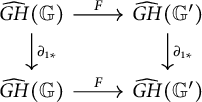
Proof Let $\pi _i:\mathit {GC}^-(\mathbb {G})\rightarrow \mathit {GC}^-(\mathbb {G})/V_i$
be the projection map.
$\pi _i:\mathit {GC}^-(\mathbb {G})\rightarrow \mathit {GC}^-(\mathbb {G})/V_i$
be the projection map.
From the previous subsection, it is sufficient to show that $\partial _1$
commutes with isomorphisms from
$\partial _1$
commutes with isomorphisms from $H(\mathit {GC}^-(\mathbb {G})/V_i)$
to
$H(\mathit {GC}^-(\mathbb {G})/V_i)$
to $H(\mathit {GC}^-(\mathbb {G})/V_j)$
(since then the arguments that
$H(\mathit {GC}^-(\mathbb {G})/V_j)$
(since then the arguments that $\partial _{1*}$
commutes with the grid move maps follows immediately).
$\partial _{1*}$
commutes with the grid move maps follows immediately).
Each such isomorphism comes from composing quasi-isomorphisms $\text {Cone}(V_i)\rightarrow \mathit {GC}^-/V_i$
induced by projection
$\text {Cone}(V_i)\rightarrow \mathit {GC}^-/V_i$
induced by projection $(c, c')\mapsto \pi _i(c'),$
and isomorphisms
$(c, c')\mapsto \pi _i(c'),$
and isomorphisms $\text {Cone}(V_i)\rightarrow \text {Cone}(V_j)$
given by
$\text {Cone}(V_i)\rightarrow \text {Cone}(V_j)$
given by $(c, c')\mapsto (c, \mathcal {H}(c)+c'),$
where
$(c, c')\mapsto (c, \mathcal {H}(c)+c'),$
where $\mathcal {H}$
is the homotopy operator from
$\mathcal {H}$
is the homotopy operator from $V_i$
to
$V_i$
to $V_j.$
By the previous subsection, we know that $\partial _{1}$
commutes with all of these maps up to homotopy (when we consider the action of
$\partial _{1}$
commutes with all of these maps up to homotopy (when we consider the action of $\partial _{1}$
on the mapping cone as
$\partial _{1}$
on the mapping cone as $\partial _1(c, c')=(\partial _1c, \partial _1c')$
), which establishes the result.
$\partial _1(c, c')=(\partial _1c, \partial _1c')$
), which establishes the result.
Now, from [Reference Ozsváth, Stipcisz and Szabó5, Chapter 7.1], we know that $\widehat {\mathit {GH}}(m(K)),$
where
$\widehat {\mathit {GH}}(m(K)),$
where $m(K)$
is the mirror of the knot
$m(K)$
is the mirror of the knot $K,$
is canonically isomorphic to the dual vector space
$K,$
is canonically isomorphic to the dual vector space $\widehat {\mathit {GH}}(K)^{\vee }.$
With a bit more work, this tells us something about the grid homology of amphicheiral knots. Using sign-refined maps, we know that we can get an invariant of knots
$\widehat {\mathit {GH}}(K)^{\vee }.$
With a bit more work, this tells us something about the grid homology of amphicheiral knots. Using sign-refined maps, we know that we can get an invariant of knots $\widehat {\mathit {GH}}(K)$
which is a module over
$\widehat {\mathit {GH}}(K)$
which is a module over $\mathbb {Z}$
. These sign-refined maps give us a knot invariant when we tensor the chain complex
$\mathbb {Z}$
. These sign-refined maps give us a knot invariant when we tensor the chain complex $\widehat {\mathit {GC}}(K)$
with
$\widehat {\mathit {GC}}(K)$
with $\mathbb {R}$
, giving us grid homology defined over the coefficient field of
$\mathbb {R}$
, giving us grid homology defined over the coefficient field of $\mathbb {R}$
. We may use the universal coefficient theorem and the sign-refined grid homology to compute grid homology defined over the coefficient field of
$\mathbb {R}$
. We may use the universal coefficient theorem and the sign-refined grid homology to compute grid homology defined over the coefficient field of $\mathbb {R}$
. We denote grid homology with
$\mathbb {R}$
. We denote grid homology with $\mathbb {R}$
coefficients as
$\mathbb {R}$
coefficients as $\widehat {\mathit {GH}}(K; \mathbb {R}).$
Lemma 7.6 If K is an amphicheiral knot, then there exists at least one nondegenerate bilinear form $\langle \cdot , \cdot \rangle $
on
$\langle \cdot , \cdot \rangle $
on $\widehat {\mathit {GH}}(K; \mathbb {R})$
for which
$\widehat {\mathit {GH}}(K; \mathbb {R})$
for which $\partial _{1*}$
is self-adjoint and the image of
$\partial _{1*}$
is self-adjoint and the image of $\partial _{1*}$
is an isotropic subspace.
$\partial _{1*}$
is an isotropic subspace.
Proof We suppress the $\mathbb {R}$
-coefficients for convenience here. The invariance of
$\mathbb {R}$
-coefficients for convenience here. The invariance of $\widehat {\mathit {GH}}$
on the grid presentation of a knot gives a bigraded isomorphism
$\widehat {\mathit {GH}}$
on the grid presentation of a knot gives a bigraded isomorphism $\Omega :\widehat {\mathit {GH}}(K)\rightarrow \widehat {\mathit {GH}}(m(K))\cong \widehat {\mathit {GH}}(K)^{\vee },$
which in turn induces such bilinear form
$\Omega :\widehat {\mathit {GH}}(K)\rightarrow \widehat {\mathit {GH}}(m(K))\cong \widehat {\mathit {GH}}(K)^{\vee },$
which in turn induces such bilinear form
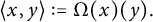 $$ \begin{align*}\langle x, y\rangle:= \Omega(x)(y).\end{align*} $$
Following the isomorphisms in [Reference Ozsváth, Stipcisz and Szabó5, Chapter 7], we see that $(\Omega (x))(\partial _{1*}y) = \Omega (\partial _{1*}x)(y),$
which proves the self-adjoint claim. Since
$(\Omega (x))(\partial _{1*}y) = \Omega (\partial _{1*}x)(y),$
which proves the self-adjoint claim. Since $\partial _{1*}^2=0,$
we get that the image of
$\partial _{1*}^2=0,$
we get that the image of $\partial _{1*}$
is an isotropic subspace.
$\partial _{1*}$
is an isotropic subspace.
Remark 7.7 We hope that, perhaps, we could prove that $\partial _{1*}$
is zero by computing the signature of one such bilinear form and showing it is positive definite, say; this would require the bilinear form to be symmetric, which is a difficult question. It is another question of interest whether this bilinear form depends on the particular isotopy of K into
$\partial _{1*}$
is zero by computing the signature of one such bilinear form and showing it is positive definite, say; this would require the bilinear form to be symmetric, which is a difficult question. It is another question of interest whether this bilinear form depends on the particular isotopy of K into $m(K).$
When K is alternating, say, then we know that $\widehat {\mathit {GH}}$
is dimension
$\widehat {\mathit {GH}}$
is dimension $\leq 1$
in each bigrading, hence the fact that
$\leq 1$
in each bigrading, hence the fact that $\Omega $
is bigraded forces each such bilinear form to be diagonal with respect to the basis consisting of nonzero homogeneous elements, hence symmetric.
$\Omega $
is bigraded forces each such bilinear form to be diagonal with respect to the basis consisting of nonzero homogeneous elements, hence symmetric.
Remark 7.8 We still have that $\partial _{1*}$
changes the grading
$\partial _{1*}$
changes the grading $(Maslov, Alexander)$
by
$(Maslov, Alexander)$
by $(-3, 0).$
A python search gives that 18 is the smallest crossing number of a prime knot with
$(-3, 0).$
A python search gives that 18 is the smallest crossing number of a prime knot with $\widehat {\mathit {GH}}$
nonzero in gradings differing by
$\widehat {\mathit {GH}}$
nonzero in gradings differing by $(-3, 0)$
.
$(-3, 0)$
.
7.3 The connection between
$\mathit {GHL}^-(K)$
and
$\tau $


Theorem 7.9 There is a spectral sequence $\{E_r, d_r\}$
of
$\{E_r, d_r\}$
of $\mathbb {F}[U]$
-modules, where
$\mathbb {F}[U]$
-modules, where $E_2 \cong \mathit {GH}^-(\mathbb {G})[v]$
and
$E_2 \cong \mathit {GH}^-(\mathbb {G})[v]$
and $d_2([\mathbf {x}]) = v\partial _{1*}([\mathbf {x}])$
, which converges to
$d_2([\mathbf {x}]) = v\partial _{1*}([\mathbf {x}])$
, which converges to $\mathit {GHL}^-(\mathbb {G})$
as
$\mathit {GHL}^-(\mathbb {G})$
as $\mathbb {F}[U]$
-modules. The
$\mathbb {F}[U]$
-modules. The $\mathbb {F}[U]$
-module isomorphism types of the terms
$\mathbb {F}[U]$
-module isomorphism types of the terms $E_n$
for
$E_n$
for $n\geq 1$
are knot invariants.
$n\geq 1$
are knot invariants.
Proof This follows immediately from the fact that the associated graded object of $\mathit {GCL}^-(\mathbb {G})$
can be expressed as the chain complex:
$\mathit {GCL}^-(\mathbb {G})$
can be expressed as the chain complex:
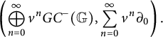 $$ \begin{align*}\left(\bigoplus_{n=0}^{\infty} v^n\mathit{GC}^-(\mathbb{G}), \sum_{n=0}^{\infty} v^n\partial_0\right).\end{align*} $$
Furthermore, unwinding definitions, it is clear that $d_2([\mathbf {x}]) = v\partial _{1*}([\mathbf {x}]).$
The spectral sequence collapses on a finite page by grading reasons. Indeed, each differential $d_r$
increases the filtration by
$d_r$
increases the filtration by $r-1$
but decreases the Maslov grading by
$r-1$
but decreases the Maslov grading by $2r-1$
; since the set of Maslov gradings for each fixed Alexander grading is finite, the sequence must collapse on a finite page.
$2r-1$
; since the set of Maslov gradings for each fixed Alexander grading is finite, the sequence must collapse on a finite page.
We now prove that $E_n$
for
$E_n$
for $n\geq 1$
are knot invariants. We know that the commutation and destabilization maps on
$n\geq 1$
are knot invariants. We know that the commutation and destabilization maps on $\mathit {GHL}^-$
all preserve the filtration. We also know that they are isomorphisms on the
$\mathit {GHL}^-$
all preserve the filtration. We also know that they are isomorphisms on the $E_2$
page of this spectral sequence, since this is simply the statement of invariance of
$E_2$
page of this spectral sequence, since this is simply the statement of invariance of $\mathit {GH}^-.$
Our desired result comes from the fact that any filtered map of filtered complexes which is an isomorphism on the
$\mathit {GH}^-.$
Our desired result comes from the fact that any filtered map of filtered complexes which is an isomorphism on the $E_2$
pages of the associated spectral sequences is an isomorphism on all higher pages of the associated spectral sequences (see [Reference McCleary4, Proposition 3.2] for a proof).
$E_2$
pages of the associated spectral sequences is an isomorphism on all higher pages of the associated spectral sequences (see [Reference McCleary4, Proposition 3.2] for a proof).
Remark 7.10 Unfortunately, we lose the structure of the v map in this spectral sequence.
Remark 7.11 This is the same proof strategy used in Rasmussen’s proof of the invariance of the Lee-Rasmussen spectral sequence in [Reference Rasmussen8].
This prompts us to define many alternatives to $\tau .$
Definition 7.12 Let K be a knot.
-
•
$\tau ^+(K)$
is
$-$
1 times the maximum Alexander grading of a U- and v-nontorsion homogeneous element in
$\mathit {GHL}^-(K).$
-
•
$\tau ^+_U(K)$
is
$-$
1 times the maximum Alexander grading of a U-nontorsion homogeneous element in
$\mathit {GHL}^-(K).$
-
•
$\rho (K)$
is the maximum k such that the equation
$U^k\xi = 0$
has a nonzero solution
$\xi \in \mathit {GHL}^-(K).$


From the spectral sequence and the definition, we immediately get the following lemma:
Lemma 7.13 For any knot K, $-\tau ^+(K)\leq -\tau ^+_U(K)\leq -\tau (K).$
Remark 7.14 As in [Reference Ozsváth, Stipcisz and Szabó5, Section 7.4], mirroring the knot K essentially dualizes the complex $\mathit {GCL}^-(K)$
over the ring
$\mathit {GCL}^-(K)$
over the ring $\mathbb {F}[U, v],$
and it would be very convenient to use this fact to prove that
$\mathbb {F}[U, v],$
and it would be very convenient to use this fact to prove that $-\tau ^+(K)=\tau ^+(m(K))$
, which in combination with the above lemma and the similar fact about
$-\tau ^+(K)=\tau ^+(m(K))$
, which in combination with the above lemma and the similar fact about $\tau ,$
would show that
$\tau ,$
would show that $\tau ^+(K)=\tau ^+_U(K)=\tau (K).$
However,
$\tau ^+(K)=\tau ^+_U(K)=\tau (K).$
However, $\mathbb {F}[U, v]$
is not a principal ideal domain, and the complications of the universal coefficient spectral sequence render this line of proof quite difficult.
$\mathbb {F}[U, v]$
is not a principal ideal domain, and the complications of the universal coefficient spectral sequence render this line of proof quite difficult.
8 Example computations with the spectral sequence
The spectral sequence defined in the previous section allows us to compute the homology $\mathit {GHL}^-(K)$
for many families of knots K by first computing
$\mathit {GHL}^-(K)$
for many families of knots K by first computing $\mathit {GH}^-(K)[v].$
In this section, we compute the examples of alternating knots and torus knots; in both examples, the spectral sequence collapses at the
$\mathit {GH}^-(K)[v].$
In this section, we compute the examples of alternating knots and torus knots; in both examples, the spectral sequence collapses at the $E_2$
page, so the computation is especially simple. The computations are therefore purely algebraic, not requiring any more topological information about the knots than the structure of
$E_2$
page, so the computation is especially simple. The computations are therefore purely algebraic, not requiring any more topological information about the knots than the structure of $\mathit {GH}^-(K).$
This provides a bit of evidence for the conjecture that $\mathit {GHL}^-(K)\cong \mathit {GH}^-(K)[v]$
always, and allows us to see examples of what
$\mathit {GHL}^-(K)\cong \mathit {GH}^-(K)[v]$
always, and allows us to see examples of what $\mathit {GHL}^-(K)$
looks like in practice.
$\mathit {GHL}^-(K)$
looks like in practice.
Theorem 8.1 If K is a quasi-alternating knot, then $\mathit {GHL}^-(K) \cong \mathit {GH}^-(K)[v]$
as bigraded
$\mathit {GHL}^-(K) \cong \mathit {GH}^-(K)[v]$
as bigraded $\mathbb {F}[U]$
-modules.
$\mathbb {F}[U]$
-modules.
Proof Let K be quasi-alternating. It is sufficient to show that the spectral sequence with $E_2$
page
$E_2$
page $\mathit {GH}^-(K)[v]$
converging to
$\mathit {GH}^-(K)[v]$
converging to $\mathit {GHL}^-(K)$
collapses at the
$\mathit {GHL}^-(K)$
collapses at the $E_2$
page.
$E_2$
page.
By [Reference Ozsváth, Stipcisz and Szabó5, Chapter 10], we know that the U-torsion part of the grid homology $\mathit {GH}^-(K)$
is supported in bigradings
$\mathit {GH}^-(K)$
is supported in bigradings $(M,A)$
with
$(M,A)$
with $M-A=-\tau ,$
and the U-nontorsion “tail” is supported in
$M-A=-\tau ,$
and the U-nontorsion “tail” is supported in $M-2A =0,$
which begins on the line
$M-2A =0,$
which begins on the line $M=A$
and extends in one direction.
$M=A$
and extends in one direction.
Hence, $\mathit {GH}^-(K)[v],$
which is what we get when we first take
$\mathit {GH}^-(K)[v],$
which is what we get when we first take $\mathit {GC}^-[v](K)$
and take homology with respect to
$\mathit {GC}^-[v](K)$
and take homology with respect to $\partial _0,$
must be supported in copies of these shapes each differing from the previous by an addition of 2 in Maslov grading. In particular, all homogeneous U-torsion elements have the same parity of their Maslov grading.
$\partial _0,$
must be supported in copies of these shapes each differing from the previous by an addition of 2 in Maslov grading. In particular, all homogeneous U-torsion elements have the same parity of their Maslov grading.
We now wish to conclude, inductively, that all the higher differentials in the spectral sequence are trivial.
If $\xi \in \mathit {GH}^-(K)[v]$
is U-torsion, then so is
$\xi \in \mathit {GH}^-(K)[v]$
is U-torsion, then so is $d_i(\xi )$
for any i by U-equivariance of the differential. Thus, any torsion elements must be in the kernel of
$d_i(\xi )$
for any i by U-equivariance of the differential. Thus, any torsion elements must be in the kernel of $d_i$
for each i since
$d_i$
for each i since $d_i$
reverses the parity of the Maslov grading.
$d_i$
reverses the parity of the Maslov grading.
Now, note that each differential in the spectral sequence increases the coefficient of v strictly. But, any point on the tail $M-2A=0$
is strictly lower in Maslov grading than any point of equal Alexander grading with a higher v coefficient. Thus, the differentials must all be zero there as well.
$M-2A=0$
is strictly lower in Maslov grading than any point of equal Alexander grading with a higher v coefficient. Thus, the differentials must all be zero there as well.
Theorem 8.2 If K is a torus knot, then $\mathit {GHL}^-(K) \cong \mathit {GH}^-(K)[v]$
as bigraded
$\mathit {GHL}^-(K) \cong \mathit {GH}^-(K)[v]$
as bigraded $\mathbb {F}[U]$
-modules.
$\mathbb {F}[U]$
-modules.
Proof Again, we show the spectral sequence collapses at $E_2,$
and we do so by analyzing the U-torsion and U-nontorsion portions separately. Let K be a positive torus knot
$E_2,$
and we do so by analyzing the U-torsion and U-nontorsion portions separately. Let K be a positive torus knot $K=T_{p,q}.$
[Reference Ozsváth, Stipcisz and Szabó5, Theorem 16.2.6] describes the structure of
$K=T_{p,q}.$
[Reference Ozsváth, Stipcisz and Szabó5, Theorem 16.2.6] describes the structure of $\widehat {\mathit {GC}}(K)$
. In particular, it shows us, by the computation that
$\widehat {\mathit {GC}}(K)$
. In particular, it shows us, by the computation that $\tau (K)=\frac {(p-1)(q-1)}2,$
that the infinite tail begins at
$\tau (K)=\frac {(p-1)(q-1)}2,$
that the infinite tail begins at $\mathbb {F}_{(\delta _{-k}, n_{-k})},$
where
$\mathbb {F}_{(\delta _{-k}, n_{-k})},$
where $n_{-k} = -\frac {(p-1)(q-1)}2.$
Per [Reference Ozsváth, Stipcisz and Szabó5, Formula 7.6], we can express $\mathit {GH}^-(K) = \mathbb {F}[U]_{(-2\tau , -\tau )}\oplus _i \mathbb {F}[U]_{(d_i, s_i)}/U^{n_i}$
. Let
$\mathit {GH}^-(K) = \mathbb {F}[U]_{(-2\tau , -\tau )}\oplus _i \mathbb {F}[U]_{(d_i, s_i)}/U^{n_i}$
. Let $\xi _i$
be the nontrivial element in
$\xi _i$
be the nontrivial element in $\mathbb {F}[U]_{(d_i, s_i)}/U^{n_i}$
that is not a multiple of
$\mathbb {F}[U]_{(d_i, s_i)}/U^{n_i}$
that is not a multiple of $U.$
Then, the
$U.$
Then, the $\xi _i$
generate the U-torsion portion of
$\xi _i$
generate the U-torsion portion of $\mathit {GH}^-(K).$
Call each such
$\mathit {GH}^-(K).$
Call each such $\mathbb {F}[U]_{(d_i, s_i)}/U^{n_i}$
a “finite tail.”
$\mathbb {F}[U]_{(d_i, s_i)}/U^{n_i}$
a “finite tail.”
Furthermore, any finite tails in $\mathit {GC}^-(K)$
contribute precisely two terms to
$\mathit {GC}^-(K)$
contribute precisely two terms to $\widehat {\mathit {GC}}(K)$
per [Reference Ozsváth, Stipcisz and Szabó5, Formula 7.6], and by this formula, we see that these finite tails must lie in higher Alexander gradings than the tail. Then, clearly any differential
$\widehat {\mathit {GC}}(K)$
per [Reference Ozsváth, Stipcisz and Szabó5, Formula 7.6], and by this formula, we see that these finite tails must lie in higher Alexander gradings than the tail. Then, clearly any differential $d_i,$
for
$d_i,$
for $i\geq 2$
, which increases the coefficient of v strictly, cannot map any point on the infinite tail to any nontrivial point. Hence, it is sufficient to consider the U-torsion parts.
$i\geq 2$
, which increases the coefficient of v strictly, cannot map any point on the infinite tail to any nontrivial point. Hence, it is sufficient to consider the U-torsion parts.
If the map $d_2$
is nontrivial on the U-torsion part, then some component of it maps some homogeneous U-torsion element
$d_2$
is nontrivial on the U-torsion part, then some component of it maps some homogeneous U-torsion element $\xi = U^k\xi _i$
to a point
$\xi = U^k\xi _i$
to a point $\zeta $
with 1 lower Maslov grading and identical Alexander grading, which is some
$\zeta $
with 1 lower Maslov grading and identical Alexander grading, which is some $U, v$
-linear combination of the
$U, v$
-linear combination of the $\xi _j.$
By grading reasons, none of the
$\xi _j.$
By grading reasons, none of the $\xi _j$
contributing nonzero terms in the expression of
$\xi _j$
contributing nonzero terms in the expression of $\zeta $
is
$\zeta $
is $\xi _i.$
The U-equivariance of
$\xi _i.$
The U-equivariance of $d_1$
tells us that at least one tail containing some
$d_1$
tells us that at least one tail containing some $\xi _j$
,
$\xi _j$
, $j\neq i,$
must terminate at the same Alexander grading
$j\neq i,$
must terminate at the same Alexander grading $A^{*}$
at which the tail containing
$A^{*}$
at which the tail containing $\xi _i$
terminates. But, this requires there to be dimension
$\xi _i$
terminates. But, this requires there to be dimension $\geq 2$
of
$\geq 2$
of $\widehat {\mathit {GC}}(K)$
at the grading
$\widehat {\mathit {GC}}(K)$
at the grading $A=A^{*},$
contradicting Theorem 16.2.6. Inductively, we may use this same argument to show
$A=A^{*},$
contradicting Theorem 16.2.6. Inductively, we may use this same argument to show $d_k$
is trivial on the U-torsion part for
$d_k$
is trivial on the U-torsion part for $k>2.$
By the construction of the spectral sequence, we must have that the sequence collapses on
$k>2.$
By the construction of the spectral sequence, we must have that the sequence collapses on $E_2,$
as desired.
$E_2,$
as desired.
A similar computation holds for negative torus knots, based on the fact that for a negative torus knot, a U-nontorsion homogeneous element of $\mathit {GH}^-(K)$
never lies in the same Alexander grading but greater Maslov grading as a U-torsion homogeneous element of
$\mathit {GH}^-(K)$
never lies in the same Alexander grading but greater Maslov grading as a U-torsion homogeneous element of $\mathit {GH}^-(K)$
.
$\mathit {GH}^-(K)$
.
Remark 8.3 These results can likely be extended without much difficulty to other classes of knots with relatively thin knot Floer homology.
9 Conclusion
It still remains open, whether the homology $\mathit {GHL}^-_S(K;\mathbb {Z})$
encodes different information than
$\mathit {GHL}^-_S(K;\mathbb {Z})$
encodes different information than $GH_S^-(K; \mathbb {Z})[v]$
. This article shows that these two objects at least obey very similar topological properties. Strategies for perhaps exhibiting an isomorphism between these two objects may relate to using the mirror of a knot, as discussed in the previous section, which may prove effective at least in showing that the nontorsion parts of these objects are isomorphic. Some of the variants of
$GH_S^-(K; \mathbb {Z})[v]$
. This article shows that these two objects at least obey very similar topological properties. Strategies for perhaps exhibiting an isomorphism between these two objects may relate to using the mirror of a knot, as discussed in the previous section, which may prove effective at least in showing that the nontorsion parts of these objects are isomorphic. Some of the variants of $\tau $
for
$\tau $
for $\mathit {GHL}^-_S(K;\mathbb {Z})$
are possibly sharper topological invariants than
$\mathit {GHL}^-_S(K;\mathbb {Z})$
are possibly sharper topological invariants than $\tau $
, so if these homologies are in fact different, we can extract useful data from our ventures.
$\tau $
, so if these homologies are in fact different, we can extract useful data from our ventures.
One pressing open question is to explore if there is an analog of the filtered theory discussed in [Reference Ozsváth, Stipcisz and Szabó5, Chapters 13 and 14] for double-point enhanced grid homology. The seemingly natural extension of the differential in this case to the double-point enhanced world is markedly not a differential anymore. If in fact, the homology $\mathit {GHL}^-_S(K;\mathbb {Z})$
is isomorphic to
$\mathit {GHL}^-_S(K;\mathbb {Z})$
is isomorphic to $GH_S^-(K; \mathbb {Z})[v]$
, then we would expect some filtered theory to exist.
$GH_S^-(K; \mathbb {Z})[v]$
, then we would expect some filtered theory to exist.
Acknowledgments
This project originated from an undergraduate summer research project at Princeton University advised by Peter Ozsváth. I would like to thank Peter Ozsváth for his advice and support throughout the project, as well as the idea for the project itself. Additionally, I would like to thank Zoltán Szabó, Isabella Khan, Matthew Kendall, Luya Wang, and Joshua Wang—who, in particular, noticed that Theorem 8.1 holds for quasi-alternating knots rather than only for alternating knots—for helpful correspondences. Thank you also to the referee for editing this paper so carefully and providing lots of helpful feedback.

 Open access