

1 Introduction
1.1 Fibrations in geometry
A general theme in the world of geometric structures is the interplay between specific geometric structures and particular types of maps. The simplest example arises in the context of fibrations, where one studies whether the presence of a geometric structure on the base and the fiber implies its existence on the total space. However, to obtain interesting spaces and geometric structures, one should allow maps to have more singularities.
A concrete case that illustrates this comes from symplectic geometry: symplectic fibrations play an important role, but they are quite rare on general symplectic manifolds. Instead, if one allows the fibration to have Lefschetz singularities, one obtains enough flexibility to establish broad existence results [Reference Donaldson13, Reference Gompf16, Reference Gompf and Stipsicz17].
In this paper, we use the point of view of decoupling the differential properties of maps from the desired underlying geometric structure. This decoupling has proved useful and allowed for several extensions of the results mentioned above, including those in [Reference Akbulut and Karakurt1–Reference Cavalcanti6, Reference Cavalcanti and Klaasse9, Reference Cavalcanti and Klaasse10, Reference Etnyre and Fuller14, Reference Gay and Kirby15, Reference Lekili23]. Here, allowing for maps to have Lefschetz and other similar singularities leads to existence results for several different types of geometric structures.
Another way in which singular fibrations arise is from proper group actions. In this setting, the “fibration” condition translates to the group action being free, which is restrictive. The quotient map of a generic action will have singularities at points with nontrivial isotropy. Such singular fibrations are particularly well studied for torus actions, $T^n\times M^{2n} \to M^{2n}$
, where, even if the actions considered are not free, they are well behaved enough to ensure that the quotient space admits the structure of a manifold with corners. The coupling of torus actions with geometric structures leads to many fruitful concepts, one of the highlights being toric geometry.
$T^n\times M^{2n} \to M^{2n}$
, where, even if the actions considered are not free, they are well behaved enough to ensure that the quotient space admits the structure of a manifold with corners. The coupling of torus actions with geometric structures leads to many fruitful concepts, one of the highlights being toric geometry.
The Lefschetz and the toric pictures come together in semitoric geometry [Reference Pelayo and Vũ Ngọc28], where maps are allowed to have both types of singularities. In this setting, the maps can have three types of singularities: elliptic, elliptic–elliptic, and focus–focus, with the latter being equivalent to Lefschetz singularities. However, in semitoric geometry, the decoupling of maps and geometric structures has happened only partially, because local singular behavior (Lefschetz and toric) and more global properties (integral affine structures) are mixed, leading to topological results [Reference Leung and Symington24].
In this paper, we introduce the differential objects hinted at by semitoric geometry: these are called self-crossing boundary (Lefschetz) fibrations (cf. Definitions 3.11 and 3.12). These types of maps incorporate local phenomena from both symplectic fibrations and quotient maps of semitoric manifolds, but do not require global structures to be present, such as group actions or integral affine structures. In this paper, we use these boundary fibrations to study an a priori seemingly unrelated geometric structure, namely a generalized complex structure.
1.2 Generalized complex structures
Generalized complex structures [Reference Gualtieri20, Reference Hitchin22] are a simultaneous generalization of symplectic and complex structures. Infinitesimally, these structures induce the product of a symplectic and complex vector space on each tangent space. However, the number of complex and symplectic directions, called the type, can vary from point to point, leading to the notion of type change. These type-changing generalized complex structures are among the most interesting to study. Within the type-changing generalized complex structures, one class was put forward in [Reference Cavalcanti and Gualtieri8, Reference Cavalcanti, Klaasse and Witte11] for being geometrically very rich and having well-controlled singular behavior: self-crossing stable generalized complex structures.
It is shown in [Reference Cavalcanti, Klaasse and Witte11] that self-crossing stable generalized complex structures on a manifold M are in one-to-one correspondence with certain Lie algebroid symplectic structures, so that this paper makes extensive use of Lie algebroids. The singularities at the type-change locus D induce a Lie algebroid $\mathcal {A}_{|D|} \to M$
called the self-crossing elliptic tangent bundle, and the generalized complex structure makes it into a symplectic Lie algebroid, carrying an elliptic symplectic structure. An elliptic symplectic structure corresponds to a self-crossing stable generalized complex structure if the locus D is co-orientable and its so-called index is
$\mathcal {A}_{|D|} \to M$
called the self-crossing elliptic tangent bundle, and the generalized complex structure makes it into a symplectic Lie algebroid, carrying an elliptic symplectic structure. An elliptic symplectic structure corresponds to a self-crossing stable generalized complex structure if the locus D is co-orientable and its so-called index is $1$
.
$1$
.
Given a self-crossing boundary Lefschetz fibration $f\colon (M,D) \to (N,Z)$
where Z is a hypersurface of N, there is another relevant Lie algebroid, namely the self-crossing log-tangent bundle
$f\colon (M,D) \to (N,Z)$
where Z is a hypersurface of N, there is another relevant Lie algebroid, namely the self-crossing log-tangent bundle $\mathcal {A}_Z \to N$
. The map f has singularities precisely such that it induces a Lie algebroid morphism
$\mathcal {A}_Z \to N$
. The map f has singularities precisely such that it induces a Lie algebroid morphism
 $$ \begin{align*} (\varphi,f)\colon (\mathcal{A}_{|D|},M) \to (\mathcal{A}_Z,N), \end{align*} $$
where $\varphi $
is now a Lie algebroid version of a Lefschetz fibration. The relevant geometric structure on the base of this fibration is a symplectic structure on
$\varphi $
is now a Lie algebroid version of a Lefschetz fibration. The relevant geometric structure on the base of this fibration is a symplectic structure on $\mathcal {A}_Z$
, also known as a self-crossing log-symplectic structure. These have also appeared in [Reference Gualtieri, Li, Pelayo and Ratiu21, Reference Miranda and Scott26]. They are compatible with the elliptic symplectic structure in the following sense.
$\mathcal {A}_Z$
, also known as a self-crossing log-symplectic structure. These have also appeared in [Reference Gualtieri, Li, Pelayo and Ratiu21, Reference Miranda and Scott26]. They are compatible with the elliptic symplectic structure in the following sense.
Definition 3.20 A self-crossing boundary fibration $f : (M,D) \rightarrow (N,Z)$
is compatible with the elliptic symplectic structure on its total space if
$f : (M,D) \rightarrow (N,Z)$
is compatible with the elliptic symplectic structure on its total space if $\ker \varphi \subseteq \mathcal {A}_{|D|}$
consists of symplectic subspaces.
$\ker \varphi \subseteq \mathcal {A}_{|D|}$
consists of symplectic subspaces.
In turn, a stable generalized complex structure is compatible with a boundary Lefschetz fibration if its induced elliptic symplectic structure is.
1.3 Results
In this section, we describe the main results obtained in this paper. In the interest of brevity, more precise versions of the results below can be found in the main body of the text.
1.3.1 Existence
Following the strategy of constructing symplectic structures out of fibrations, we prove a Gompf–Thurston theorem for self-crossing stable generalized complex structures. This result is the generalization of a similar result for stable generalized complex structures with embedded type-change locus appearing in [Reference Cavalcanti and Klaasse9], but requires several adaptations of the argument.
Definition 3.19 A boundary Lefschetz fibration, $f\colon (M^4,D) \to (N^2,Z)$
, is homologically essential if the homology class
$f\colon (M^4,D) \to (N^2,Z)$
, is homologically essential if the homology class $[F]$
of the fiber of
$[F]$
of the fiber of $f\colon M \backslash D \rightarrow N \backslash Z$
is nontrivial in
$f\colon M \backslash D \rightarrow N \backslash Z$
is nontrivial in $H_2(M\backslash D;\mathbb {R})$
.
$H_2(M\backslash D;\mathbb {R})$
.
Theorem 3.23 Let $f\colon (M^4,D^2) \rightarrow (N^2,\partial N)$
be a homologically essential self-crossing boundary Lefschetz fibration. Then
$f\colon (M^4,D^2) \rightarrow (N^2,\partial N)$
be a homologically essential self-crossing boundary Lefschetz fibration. Then $M^4$
admits an elliptic symplectic structure compatible with f, which induces a self-crossing stable generalized complex structure compatible with f if the locus D is co-orientable and its index is equal to
$M^4$
admits an elliptic symplectic structure compatible with f, which induces a self-crossing stable generalized complex structure compatible with f if the locus D is co-orientable and its index is equal to $1$
.
$1$
.
1.3.2 Construction
Having established that boundary Lefschetz fibrations supply self-crossing stable generalized complex structures, we decouple the map from the geometric structure and study them separately. These types of maps are flexible enough to admit connected sums.
Theorem 4.6 Let $f_i\colon (M_i^4,D_i^2) \rightarrow (N_i^2,\partial N_i)$
, for
$f_i\colon (M_i^4,D_i^2) \rightarrow (N_i^2,\partial N_i)$
, for $i = 1,2$
, be boundary Lefschetz fibrations, and let
$i = 1,2$
, be boundary Lefschetz fibrations, and let $p_i \in M_i$
be such that
$p_i \in M_i$
be such that $q_i = f_i(p_i)$
are corners of the manifolds
$q_i = f_i(p_i)$
are corners of the manifolds $N_i$
. Then there exists a boundary Lefschetz fibration on their connected sum,
$N_i$
. Then there exists a boundary Lefschetz fibration on their connected sum,
 $$ \begin{align*} f_1 \# f_2\colon (M_1 \#_{p_1,p_2}M_2,D_1 \# D_2) \rightarrow (N_1\#_{q_1,q_2}N_2,\partial (N_1\# N_2)), \end{align*} $$
which is compatible with the inclusion $M_i \backslash \lbrace p_i \rbrace \hookrightarrow M_1 \# M_2$
. Moreover, the map
$M_i \backslash \lbrace p_i \rbrace \hookrightarrow M_1 \# M_2$
. Moreover, the map $f_1 \# f_2$
is homologically essential if and only if
$f_1 \# f_2$
is homologically essential if and only if $f_1$
and
$f_1$
and $f_2$
are.
$f_2$
are.
This result is in sheer contrast with the situation in toric geometry. There is no symplectic connected sum procedure, and most of the manifolds obtained using the above proposition will have no toric structure. This difference in rigidity between the generalized complex and toric worlds is already apparent on the base of these fibrations. Namely, for generalized complex structures, the base carries a self-crossing log-symplectic structure, which is quite flexible. On the other hand, in toric geometry, the base carries an integral affine structure, which is very rigid. In other words, although toric manifolds do not behave well with respect to connected sums, the underlying torus actions and abstract quotient maps do.
1.3.3 Singularity trades
The nodal-trade procedure in semitoric geometry exchanges elliptic–elliptic singularities of the moment map for focus–focus singularities [Reference van der Meer32, Reference Zung33] and vice-versa [Reference Leung and Symington24]. These procedures rely heavily on the existence of a singular integral affine structure on the base. Following our general strategy, decoupling the geometric structure from the maps allows us to prove an abstract statement for boundary Lefschetz fibrations.
Theorem 5.3 Let $f\colon (M^4,D^2) \rightarrow (N^2,\partial N)$
be a boundary Lefschetz fibration, and let
$f\colon (M^4,D^2) \rightarrow (N^2,\partial N)$
be a boundary Lefschetz fibration, and let $p \in M$
be an elliptic–elliptic singularity. Then there exists a boundary Lefschetz fibration
$p \in M$
be an elliptic–elliptic singularity. Then there exists a boundary Lefschetz fibration
 $$ \begin{align*} {\widetilde{f}\colon (M,\widetilde{D}) \rightarrow (\widetilde{N},\partial \widetilde{N})} \end{align*} $$
agreeing with f outside a neighborhood of p, and such that the elliptic–elliptic singularity is traded for a Lefschetz singularity. The map $\widetilde {f}$
is homologically essential if and only if f is.
$\widetilde {f}$
is homologically essential if and only if f is.
The proof of this result, and its converse, Theorem 5.4, relies on the connected sum procedure and the existence of a particular boundary Lefschetz fibration on $S^4$
. Figure 1 illustrates the singularity trade from Theorem 5.3 in
$S^4$
. Figure 1 illustrates the singularity trade from Theorem 5.3 in $\mathbb{C}P^2$
.
$\mathbb{C}P^2$
.
1.3.4 Examples
Using simple manifolds as building blocks, the connected sum procedure allows us to construct many examples of boundary Lefschetz fibrations (and consequently of self-crossing stable generalized complex structures) on the following manifolds.
Theorem 6.12 The manifolds in the following two families:
-
• $X_{n,\ell } := \#n(S^2\times S^2)\#\ell (S^1\times S^3)$
, with
$n,\ell \in \mathbb {N}$
,
$X_{n,\ell } := \#n(S^2\times S^2)\#\ell (S^1\times S^3)$
, with
$n,\ell \in \mathbb {N}$
, -
•
$Y_{n,m,\ell } := \#n \mathbb {C} P^2 \#m \overline {\mathbb {C}P}^2\#\ell (S^1 \times S^3)$
, with
$n,m,\ell \in \mathbb {N}$
,


admit homologically essential boundary Lefschetz fibrations whenever their Euler characteristic is nonnegative. Therefore, each of these manifolds admits a compatible elliptic symplectic structure, which induces a self-crossing stable generalized complex structure if $1-b_1 + b_2^+$
is even.
$1-b_1 + b_2^+$
is even.
Combining this result with Theorem 5.3, we conclude that the above manifolds moreover admit stable generalized complex structures with embedded degeneracy loci. These examples have already appeared in the literature [Reference Cavalcanti and Gualtieri7, Reference Goto and Hayano18, Reference Torres30, Reference Torres and Yazinski31], and the authors obtained them as well in [Reference Cavalcanti, Klaasse and Witte11, Theorem 7.5]. However, the above result shows that the structures in these examples can be made compatible with boundary Lefschetz fibrations. This gives us much more control about stable generalized complex structures in concrete applications. For instance, we believe it will help in the development of a Fukaya category for stable generalized complex structures just like ordinary Lefschetz fibrations can be used to understand the Fukaya category of symplectic manifolds [Reference Seidel29].
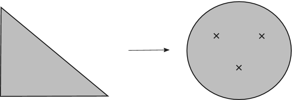
Figure 1: The picture on the left presents $\mathbb {C} P^2$
using the usual moment map, which is the prototypical example of a self-crossing boundary fibration. Theorem 5.3 tells us that we can slightly modify this fibration to obtain a boundary Lefschetz fibration, with three Lefschetz singularities.
$\mathbb {C} P^2$
using the usual moment map, which is the prototypical example of a self-crossing boundary fibration. Theorem 5.3 tells us that we can slightly modify this fibration to obtain a boundary Lefschetz fibration, with three Lefschetz singularities.
1.4 Organization of the paper
This paper is organized as follows. In Section 2, we recall from [Reference Cavalcanti, Klaasse and Witte11] the notions of self-crossing divisors, and their associated Lie algebroids and symplectic structures. We also recall the definition of self-crossing stable generalized complex structures and that they are in one-to-one correspondence with particular self-crossing elliptic symplectic structures. In Section 3, we extend the notion of boundary (Lefschetz) fibration from [Reference Cavalcanti and Klaasse9] to allow for self-crossing of the degeneracy locus. We moreover prove the Gompf–Thurston result, Theorem 3.23. In Section 4, we show that boundary Lefschetz fibrations allow for taking connected sums and prove Theorem 4.6. In Section 5, we will prove the singularity trade results, namely Theorems 5.3 and 5.4. Finally, in Section 6, we show that torus actions give rise to boundary fibrations, and exhibit several examples, including Theorem 6.12 and Proposition 6.9.
2 Divisors, Lie algebroids, and symplectic structures
In this section, we study geometric structures with specific singularities. To work with these singularities, we will recall the concept of a divisor, and the particular cases of log and elliptic divisors which we will mainly use in this paper. Using these divisors, we will recall the associated Lie algebroids and their Lie algebroid symplectic structures. Then we will introduce the objects which we want to construct in this paper, namely stable generalized complex structures. We will show that these structures correspond to certain Lie algebroid symplectic structures, which is how we will treat them in the rest of the paper.
2.1 Divisors
We will use an adaptation of the notion of a divisor from algebraic geometry to smooth manifolds in order to describe the singularities of geometric structures. We will only briefly go over the main concepts we need and refer to [Reference Cavalcanti and Gualtieri8, Reference Cavalcanti and Klaasse9, Reference Cavalcanti, Klaasse and Witte11] for more information.
Definition 2.1 A real/complex divisor on M is a locally principal ideal I of $C^{\infty }(M;\mathbb {R})$
, respectively,
$C^{\infty }(M;\mathbb {R})$
, respectively, $C^{\infty }(M;\mathbb {C})$
, which is locally generated by functions with nowhere dense zero set.
$C^{\infty }(M;\mathbb {C})$
, which is locally generated by functions with nowhere dense zero set.
Equivalently, divisors can be described as follows.
Proposition 2.2 Let I be a real/complex divisor on M. Then there exists a real/complex line bundle $L \rightarrow M$
with section
$L \rightarrow M$
with section $\sigma \in \Gamma (L)$
such that
$\sigma \in \Gamma (L)$
such that $\sigma (\Gamma (L^*)) = I$
.
$\sigma (\Gamma (L^*)) = I$
.
Note that the line bundle L is uniquely determined up to vector bundle isomorphism (covering the identity), and that the section $\sigma $
is unique up to multiplication by a smooth function. Given a pair
$\sigma $
is unique up to multiplication by a smooth function. Given a pair $(L,\sigma )$
, we denote the associated divisor by
$(L,\sigma )$
, we denote the associated divisor by $I_{\sigma }$
.
$I_{\sigma }$
.
Definition 2.3 Let $(M,I_M)$
and
$(M,I_M)$
and $(N,I_N)$
be manifolds with divisors. A smooth map
$(N,I_N)$
be manifolds with divisors. A smooth map $\varphi \colon M \rightarrow N$
is a morphism of divisors if
$\varphi \colon M \rightarrow N$
is a morphism of divisors if $\varphi ^*I_N = I_M$
, where the left-hand side denotes the ideal generated by all pullbacks. It is called a diffeomorphism of divisors if
$\varphi ^*I_N = I_M$
, where the left-hand side denotes the ideal generated by all pullbacks. It is called a diffeomorphism of divisors if $\varphi $
is a diffeomorphism.
$\varphi $
is a diffeomorphism.
Definition 2.4 A smooth real/complex log divisor is a real/complex divisor I locally generated by transverse vanishing functions.
The vanishing locus of a real log divisor has codimension 1 and is denoted by Z. The vanishing locus of a complex log divisor has codimension 2 and is denoted by D. By locally demanding a divisor to be a product of log divisors, we obtain the following.
Definition 2.5 A self-crossing real/complex log divisor on a manifold M is a divisor I, such that for every point $p\in M$
, there exists a neighborhood U of p such that
$p\in M$
, there exists a neighborhood U of p such that
 $$ \begin{align*} I(U) = I_1\cdot \ldots \cdot I_j, \end{align*} $$
where $I_1,\ldots ,I_j$
are real/complex log ideals with transversely intersecting vanishing loci.
$I_1,\ldots ,I_j$
are real/complex log ideals with transversely intersecting vanishing loci.
Example 2.6 There is a standard example for each of the divisor types described above.
-
The standard real log divisor on
$\mathbb {R}^j \times \mathbb {R}^m$
is defined using the coordinates
$(x_1,\ldots , x_j,y_i)$
by the ideal
$I_Z := \left \langle x_1\cdot \ldots \cdot x_j \right \rangle $
; -
The standard complex log divisor on
$\mathbb {C}^j \times \mathbb {R}^m$
is defined using the coordinates
$(z_1,\ldots , z_j,y_i)$
by the ideal
$I_D := \left \langle z_1\cdot \ldots \cdot z_j \right \rangle $
.


Each of these examples provides the local normal form for their associated divisor type.
A self-crossing real log divisor is determined by its vanishing locus Z, as its ideal equals the ideal of functions vanishing on Z. In contrast, for a self-crossing complex log divisor, the subspace D does not determine the divisor.
Definition 2.7 [Reference Cavalcanti and Gualtieri8]
A smooth elliptic divisor is a real divisor $I_{\left | D \right |}$
locally generated by definite Morse–Bott functions with codimension-2 critical set.
$I_{\left | D \right |}$
locally generated by definite Morse–Bott functions with codimension-2 critical set.
In fact, asking the existence of local generating function of $I_{\left | D \right |}$
as above implies that there exists a global generator
$I_{\left | D \right |}$
as above implies that there exists a global generator $f \in I_{\left | D \right |}$
.
$f \in I_{\left | D \right |}$
.
Again by taking appropriate products, we obtain the following.
Definition 2.8 [Reference Cavalcanti, Klaasse and Witte11]
A self-crossing elliptic divisor is a divisor $I_{\left | D \right |}$
on a manifold M, such that for every point
$I_{\left | D \right |}$
on a manifold M, such that for every point $p\in M$
, there exists a neighborhood U of p such that
$p\in M$
, there exists a neighborhood U of p such that
 $$ \begin{align*} I_{\left| D \right|}(U) = I_1\cdot \ldots \cdot I_j, \end{align*} $$
where the $I_1,\ldots ,I_j$
are smooth elliptic divisors with transversely intersecting vanishing loci.
$I_1,\ldots ,I_j$
are smooth elliptic divisors with transversely intersecting vanishing loci.
Example 2.9 The standard elliptic divisor on $\mathbb {R}^{2j} \times \mathbb {R}^m$
is defined using the coordinates
$\mathbb {R}^{2j} \times \mathbb {R}^m$
is defined using the coordinates $(x_1,y_1,\ldots , x_j,y_j,u_i)$
by the ideal
$(x_1,y_1,\ldots , x_j,y_j,u_i)$
by the ideal $I_{\left | D \right |} := \left \langle (x_1^2+y_1^2)\cdot \ldots \cdot (x_j^2+y_j^2) \right \rangle $
. Lemma 2.23 in [Reference Cavalcanti, Klaasse and Witte11] ensures that any self-crossing elliptic divisor is of this form.
$I_{\left | D \right |} := \left \langle (x_1^2+y_1^2)\cdot \ldots \cdot (x_j^2+y_j^2) \right \rangle $
. Lemma 2.23 in [Reference Cavalcanti, Klaasse and Witte11] ensures that any self-crossing elliptic divisor is of this form.
As for smooth elliptic divisors, the ideal $I_{\left | D \right |}$
is generated by a single global function
$I_{\left | D \right |}$
is generated by a single global function $f \colon M \to \mathbb {R}_+$
, which by Example 2.9 is locally of the form
$f \colon M \to \mathbb {R}_+$
, which by Example 2.9 is locally of the form
 $$ \begin{align*} f(x_1,y_1,\dots,x_j,y_j,x_{k+1},\dots, x_{n}) = (x_1^2 + y_1^2)\dots (x_j^2 + y_j^2). \end{align*} $$
We mostly deal with self-crossing divisors in this paper, and we will often omit the prefix “self-crossing.” Whenever we mean a smooth log or elliptic divisor, we will explicitly stress this.
The vanishing loci of both log and elliptic divisors are not embedded, but are stratified.
Definition 2.10 Let I be a real/complex log or elliptic divisor on M with vanishing locus D. The multiplicity of a point $p \in M$
is the minimum of the integers j from Definitions 2.5 or 2.8 over all neighborhoods U of p. If I has points of multiplicity at most n, the sets
$p \in M$
is the minimum of the integers j from Definitions 2.5 or 2.8 over all neighborhoods U of p. If I has points of multiplicity at most n, the sets $D(j)$
of points of multiplicity at least j induce a filtration of M:
$D(j)$
of points of multiplicity at least j induce a filtration of M:
 $$ \begin{align*} M = D(0) \supset D(1) = D \supset \cdots \supset D(n), \end{align*} $$
with induced stratification with strata $D[j]$
of points with multiplicity precisely j.
$D[j]$
of points with multiplicity precisely j.
That this is a stratification follows readily from the normal forms of the divisors in Examples 2.6 and 2.9. Also, note that if a divisor I has multiplicity n and $i \leq n$
is given, then the restriction
$i \leq n$
is given, then the restriction $\left .{I}\right |{}_{M\backslash D(i+1)}$
defines a divisor with multiplicity i.
$\left .{I}\right |{}_{M\backslash D(i+1)}$
defines a divisor with multiplicity i.
Example 2.11 Another important example for this paper is a manifold with corners $(M,\partial M)$
. The boundary of a manifold with corners naturally defines a real log divisor.
$(M,\partial M)$
. The boundary of a manifold with corners naturally defines a real log divisor.
Given a self-crossing complex log divisor $I_D$
, its associated (self-crossing) elliptic divisor is the real divisor
$I_D$
, its associated (self-crossing) elliptic divisor is the real divisor $I_{\left | D \right |}$
defined by
$I_{\left | D \right |}$
defined by $I_{\left | D \right |} \otimes \mathbb {C} = I_D \otimes \overline {I_D}$
.
$I_{\left | D \right |} \otimes \mathbb {C} = I_D \otimes \overline {I_D}$
.
2.2 Lie algebroids and residue maps
Each of the divisors introduced in the previous section gives rise to a corresponding Lie algebroid via the Serre–Swan theorem and the local normal forms contained in Examples 2.6 and 2.9.
Definition 2.12 Let $I_Z$
be a real log divisor,
$I_Z$
be a real log divisor, $I_D$
a complex log divisor, and
$I_D$
a complex log divisor, and $I_{\left | D \right |}$
be an elliptic divisor. The vector fields preserving each of these ideals define Lie algebroids:
$I_{\left | D \right |}$
be an elliptic divisor. The vector fields preserving each of these ideals define Lie algebroids:
-
•
$\mathcal {A}_Z \to TM$
, the real log-tangent bundle associated to
$I_Z$
; -
•
$\mathcal {A}_D \to T_{\mathbb {C}} M$
, the complex log-tangent bundle associated to
$I_D$
; and -
•
$\mathcal {A}_{\left | D \right |} \to TM$
, the elliptic tangent bundle associated to
$I_{\left | D \right |}$
.


Remark 2.13 The above Lie algebroids can be described in the local coordinates of in Examples 2.6 and 2.9. Indeed, around a point of multiplicity j, we have:
-
•
$\Gamma (\mathcal {A}_Z) = \left \langle x_1\partial _{x_1},\ldots ,x_j\partial _{x_j},\partial _{y_i} \right \rangle $
; -
•
$\Gamma (\mathcal {A}_D) = \left \langle z_1\partial _{z_1},\partial _{\overline {z}_1},\ldots ,z_j\partial _{z_j},\partial _{\overline {z}_j},\partial _{y_i} \right \rangle $
; and -
•
$\Gamma (\mathcal {A}_{\left | D \right |}) = \left \langle r_1\partial _{r_1},\partial _{\theta _i}, \ldots ,r_j\partial _{r_j},\partial _{\theta _j},\partial _{u_i} \right \rangle $
.


In the latter case, we have $r_i\partial _{r_i} := x_i\partial _{x_i}+y_i\partial _{y_i}$
and
$r_i\partial _{r_i} := x_i\partial _{x_i}+y_i\partial _{y_i}$
and $\partial _{\theta _i} := x_i\partial _{y_i}-y_i\partial _{x_i}$
.
$\partial _{\theta _i} := x_i\partial _{y_i}-y_i\partial _{x_i}$
.
When $I_D$
is a complex log divisor on M and
$I_D$
is a complex log divisor on M and $I_{\left | D \right |}$
is its associated elliptic divisor, there is a fiber product relation between the corresponding Lie algebroids as follows:
$I_{\left | D \right |}$
is its associated elliptic divisor, there is a fiber product relation between the corresponding Lie algebroids as follows:
 $$ \begin{align*} \mathcal{A}_{D} \times_{T_{\mathbb{C}}M} \mathcal{A}_{\overline{D}} \cong \mathcal{A}_{\left| D \right|} \otimes \mathbb{C}. \end{align*} $$
This isomorphism provides an inclusion $\iota ^*\colon \Omega ^{\bullet }(\mathcal {A}_D) \to \Omega ^{\bullet }_{\mathbb {C}}(\mathcal {A}_{\left | D \right |})$
.
$\iota ^*\colon \Omega ^{\bullet }(\mathcal {A}_D) \to \Omega ^{\bullet }_{\mathbb {C}}(\mathcal {A}_{\left | D \right |})$
.
We now turn to describing several of the residue maps carried by these Lie algebroids. Let $(I_{\left | D \right |},\mathfrak {o})$
be a smooth elliptic divisor, together with a co-orientation of D. As explained in [Reference Cavalcanti and Gualtieri8], the elliptic tangent bundle has an elliptic and radial residue map. These are maps of cochain complexes, and they extract the coefficients of the singular generators. In the coordinates of Remark 2.13, these are given by
$(I_{\left | D \right |},\mathfrak {o})$
be a smooth elliptic divisor, together with a co-orientation of D. As explained in [Reference Cavalcanti and Gualtieri8], the elliptic tangent bundle has an elliptic and radial residue map. These are maps of cochain complexes, and they extract the coefficients of the singular generators. In the coordinates of Remark 2.13, these are given by
 $$ \begin{align} \begin{aligned} \operatorname{\mathrm{Res}}_q\colon \Omega^{\bullet}(\mathcal{A}_{\left| D \right|}) \rightarrow \Omega^{\bullet-2}(D),& \qquad \operatorname{\mathrm{Res}}_q(\alpha)= \iota^*_D(\iota_{r\partial_r\wedge\partial_{\theta}}\alpha),\\ \operatorname{\mathrm{Res}}_r\colon \Omega^{\bullet}(\mathcal{A}_{\left| D \right|}) \rightarrow \Omega^{\bullet-1}(S^1ND),&\qquad \operatorname{\mathrm{Res}}_r(\alpha) = \iota^*_D(\iota_{r\partial_r}\alpha), \end{aligned} \end{align} $$
where $S^1ND \to D$
is the
$S^1ND \to D$
is the $S^1$
-bundle associated to the co-orientation
$S^1$
-bundle associated to the co-orientation $\mathfrak {o}$
of D.
$\mathfrak {o}$
of D.
These residue maps can be extended to self-crossing elliptic divisors if we restrict our attention to the stratum $D[1]$
. We say that a self-crossing elliptic divisor is co-oriented if the normal bundle
$D[1]$
. We say that a self-crossing elliptic divisor is co-oriented if the normal bundle $ND[1] \to D[1]$
is oriented.
$ND[1] \to D[1]$
is oriented.
Definition 2.14 Let $(I_{\left | D \right |},\mathfrak {o})$
be a self-crossing elliptic divisor together with a co-orientation
$(I_{\left | D \right |},\mathfrak {o})$
be a self-crossing elliptic divisor together with a co-orientation $\mathfrak {o}$
of
$\mathfrak {o}$
of $D[1]$
. The elliptic and radial residues of
$D[1]$
. The elliptic and radial residues of $\alpha \in \Omega ^{\bullet }(\mathcal {A}_{\left | D \right |})$
are
$\alpha \in \Omega ^{\bullet }(\mathcal {A}_{\left | D \right |})$
are $\operatorname {\mathrm {Res}}_q(\alpha ) := \operatorname {\mathrm {Res}}_q(\iota ^*_{D[1]}\alpha )$
and
$\operatorname {\mathrm {Res}}_q(\alpha ) := \operatorname {\mathrm {Res}}_q(\iota ^*_{D[1]}\alpha )$
and $\operatorname {\mathrm {Res}}_r(\alpha ) := \operatorname {\mathrm {Res}}_r(\iota ^*_{D[1]}\alpha )$
.
$\operatorname {\mathrm {Res}}_r(\alpha ) := \operatorname {\mathrm {Res}}_r(\iota ^*_{D[1]}\alpha )$
.
In later constructions, the cohomology of the complex of forms with vanishing radial residue will play a role.
Lemma 2.15 Let $I_{\left | D \right |}$
be a self-crossing elliptic divisor on a manifold M, and let
$I_{\left | D \right |}$
be a self-crossing elliptic divisor on a manifold M, and let $\Omega _{0,0}^{\bullet }(\mathcal {A}_{\left | D \right |}) \subset \Omega ^{\bullet }(\mathcal {A}_{\left | D \right |})$
be the subcomplex defined as the kernel of the map
$\Omega _{0,0}^{\bullet }(\mathcal {A}_{\left | D \right |}) \subset \Omega ^{\bullet }(\mathcal {A}_{\left | D \right |})$
be the subcomplex defined as the kernel of the map $\operatorname {\mathrm {Res}}_r$
. Then the inclusion map
$\operatorname {\mathrm {Res}}_r$
. Then the inclusion map $\iota \colon M\backslash D \to M$
of the complement of D induces a quasi-isomorphism
$\iota \colon M\backslash D \to M$
of the complement of D induces a quasi-isomorphism $\iota ^*\colon \Omega ^{\bullet }_{0,0}(\mathcal {A}_{\left | D \right |}) \rightarrow \Omega ^{\bullet }(M\backslash D)$
.
$\iota ^*\colon \Omega ^{\bullet }_{0,0}(\mathcal {A}_{\left | D \right |}) \rightarrow \Omega ^{\bullet }(M\backslash D)$
.
Proof The argument uses the observation from [Reference Grothendieck19, Theorem 1.2] (and the fact that $\mathcal {A}_{\left | D \right |}$
defines a soft sheaf) that it suffices to show that
$\mathcal {A}_{\left | D \right |}$
defines a soft sheaf) that it suffices to show that $\iota ^*$
induces an isomorphism on the level of sheaf cohomology. Below we will implicitly identify the sheaf
$\iota ^*$
induces an isomorphism on the level of sheaf cohomology. Below we will implicitly identify the sheaf $\Omega ^{\bullet }(M\backslash D)$
with its push-forward
$\Omega ^{\bullet }(M\backslash D)$
with its push-forward $\iota _*(\Omega ^{\bullet }(M\backslash D))$
. For all points
$\iota _*(\Omega ^{\bullet }(M\backslash D))$
. For all points $p \in M\backslash D$
, there exists a contractible open neighborhood U of p disjoint from D. On this open
$p \in M\backslash D$
, there exists a contractible open neighborhood U of p disjoint from D. On this open $\mathcal {A}_{\left | D \right |} = TM$
and
$\mathcal {A}_{\left | D \right |} = TM$
and $\operatorname {\mathrm {Res}}_r \equiv 0$
, and therefore
$\operatorname {\mathrm {Res}}_r \equiv 0$
, and therefore $\iota _*$
is simply the identity. Let j be any integer less than or equal to the point of highest multiplicity of D, take
$\iota _*$
is simply the identity. Let j be any integer less than or equal to the point of highest multiplicity of D, take $p \in D[j]$
, and let U be a contractible open around p as in Remark 2.13. In those coordinates,
$p \in D[j]$
, and let U be a contractible open around p as in Remark 2.13. In those coordinates, $H^{\bullet }_{0,0}(U,\mathcal {A}_{\left | D \right |})$
is the free algebra generated by
$H^{\bullet }_{0,0}(U,\mathcal {A}_{\left | D \right |})$
is the free algebra generated by $\lbrace 1,d\theta _1,\ldots ,d\theta _j \rbrace $
. By an elementary argument,
$\lbrace 1,d\theta _1,\ldots ,d\theta _j \rbrace $
. By an elementary argument, $U\backslash D$
is homotopic to
$U\backslash D$
is homotopic to $\mathbb {T}^j$
, and using this homotopy
$\mathbb {T}^j$
, and using this homotopy $\iota ^*$
takes the generators of
$\iota ^*$
takes the generators of $H^{\bullet }_{0,0}(\mathcal {A}_{\left | D \right |})$
to the generators of
$H^{\bullet }_{0,0}(\mathcal {A}_{\left | D \right |})$
to the generators of $H^{\bullet }(U\backslash D)$
. Therefore, we conclude that
$H^{\bullet }(U\backslash D)$
. Therefore, we conclude that $\iota ^*$
is a local isomorphism, and consequently a global isomorphism.▪
$\iota ^*$
is a local isomorphism, and consequently a global isomorphism.▪
We will need a few more residue maps for self-crossing elliptic divisors.
Definition 2.16 [Reference Cavalcanti, Klaasse and Witte11]
Let $(I_{\left | D \right |},\mathfrak {o})$
be a co-oriented elliptic divisor, and let
$(I_{\left | D \right |},\mathfrak {o})$
be a co-oriented elliptic divisor, and let $\omega \in \Omega ^2(\mathcal {A}_{\left | D \right |})$
. Let
$\omega \in \Omega ^2(\mathcal {A}_{\left | D \right |})$
. Let $p \in D(k)$
with
$p \in D(k)$
with $k\geq 2$
and consider oriented coordinates as in Remark 2.13. We define
$k\geq 2$
and consider oriented coordinates as in Remark 2.13. We define
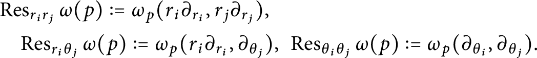 $$ \begin{align*} &\operatorname{\mathrm{Res}}_{r_ir_j}\omega(p) := \omega_p(r_i\partial_{r_i},r_j\partial_{r_j}), \\ &\quad \operatorname{\mathrm{Res}}_{r_i\theta_j}\omega(p) := \omega_p(r_i\partial_{r_i},\partial_{\theta_j}),~ \operatorname{\mathrm{Res}}_{\theta_i\theta_j}\omega(p) := \omega_p(\partial_{\theta_i},\partial_{\theta_j}). \end{align*} $$
These pointwise expressions depend on $\mathfrak {o}$
and the ordering of coordinates, but only up to sign.
$\mathfrak {o}$
and the ordering of coordinates, but only up to sign.
2.3 Lie algebroid symplectic structures
We will use the language of symplectic Lie algebroids to translate certain Poisson and generalized complex structures into simpler Lie algebroid objects. Given a Lie algebroid two-form $\omega \in \Omega ^2(\mathcal {A})$
, we say it is nondegenerate if
$\omega \in \Omega ^2(\mathcal {A})$
, we say it is nondegenerate if $\omega ^{\flat }\colon \mathcal {A} \rightarrow \mathcal {A}^*$
is an isomorphism.
$\omega ^{\flat }\colon \mathcal {A} \rightarrow \mathcal {A}^*$
is an isomorphism.
Definition 2.17 Let $I_Z$
and
$I_Z$
and $I_{|D|}$
be real log and elliptic divisors on a given manifold M. Then:
$I_{|D|}$
be real log and elliptic divisors on a given manifold M. Then:
-
• A form
$\omega \in \Omega ^2(\mathcal {A}_Z)$
is log-symplectic if
$d \omega = 0$
and it is nondegenerate. -
• A form
$\omega \in \Omega ^2(\mathcal {A}_{|D|})$
is elliptic symplectic if
$d\omega = 0$
and it is nondegenerate.


One can prove Darboux-type normal form theorems for symplectic Lie algebroids using a thorough understanding of their Lie algebroid cohomology, by a straightforward adaptation of the Moser lemma. However, in the above cases, this cohomology is generally locally nontrivial, so that there is no unique local model. In dimension 2, we have the following (which is the real analogue of Proposition 5.2 in [Reference Cavalcanti, Klaasse and Witte11]).
Lemma 2.18 Let $I_Z$
be a real log divisor on
$I_Z$
be a real log divisor on $\Sigma ^2$
, and let
$\Sigma ^2$
, and let $\omega \in \Omega ^2(\mathcal {A}_Z)$
be a log-symplectic form. For each point
$\omega \in \Omega ^2(\mathcal {A}_Z)$
be a log-symplectic form. For each point $p \in Z[2]$
, there are coordinates
$p \in Z[2]$
, there are coordinates $(x_1,x_2)$
centered at p and
$(x_1,x_2)$
centered at p and $\lambda \in \mathbb {R}$
such that
$\lambda \in \mathbb {R}$
such that
 $$ \begin{align*} \omega = \lambda d\log x_1 \wedge d\log x_2. \end{align*} $$
Since in two dimensions every nowhere zero two-form is closed and nondegenerate, we have the following source of examples of log-symplectic manifolds.
Lemma 2.19 Let $\Sigma ^2$
be a compact oriented surface with corners. Then
$\Sigma ^2$
be a compact oriented surface with corners. Then $(\Sigma ,I_{\partial \Sigma })$
admits a log-symplectic structure.
$(\Sigma ,I_{\partial \Sigma })$
admits a log-symplectic structure.
Proof The ideal $I_{\partial \Sigma }$
defines a real log divisor. Because
$I_{\partial \Sigma }$
defines a real log divisor. Because $\Sigma $
is oriented, let
$\Sigma $
is oriented, let $h \in C^{\infty }(M)$
be a defining function for
$h \in C^{\infty }(M)$
be a defining function for $\partial M$
, so that
$\partial M$
, so that $I_{\partial \Sigma } = \langle h \rangle $
, and let
$I_{\partial \Sigma } = \langle h \rangle $
, and let $\omega \in \Omega ^2(\Sigma )$
be a volume form. Then
$\omega \in \Omega ^2(\Sigma )$
be a volume form. Then $h^{-1}\omega \in \Omega ^2(\mathcal {A}_{\partial M})$
is a nondegenerate log two-form that is closed for dimensional reasons.▪
$h^{-1}\omega \in \Omega ^2(\mathcal {A}_{\partial M})$
is a nondegenerate log two-form that is closed for dimensional reasons.▪
2.4 Self-crossing stable generalized complex structures
In this section, we recall the notion of a self-crossing stable generalized complex structure [Reference Cavalcanti, Klaasse and Witte11]. This is a well-behaved class of generalized complex structures [Reference Gualtieri20], i.e., complex structures on the bundle $\mathbb {T}M:= TM \oplus T^*M$
. We furthermore recall that they are equivalent to certain elliptic symplectic structures.
$\mathbb {T}M:= TM \oplus T^*M$
. We furthermore recall that they are equivalent to certain elliptic symplectic structures.
Definition 2.20 A generalized complex structure on a manifold M is a pair $(\mathbb {J},H)$
where
$(\mathbb {J},H)$
where $H \in \Omega ^3(M)$
is a closed three-form and
$H \in \Omega ^3(M)$
is a closed three-form and $\mathbb {J}$
is a skew-symmetric endomorphism of
$\mathbb {J}$
is a skew-symmetric endomorphism of $\mathbb {T}M$
for which
$\mathbb {T}M$
for which $\mathbb {J}^2 = -\rm {Id}$
and the
$\mathbb {J}^2 = -\rm {Id}$
and the $+i$
-eigenbundle,
$+i$
-eigenbundle, $L \subset (\mathbb {T}M) \otimes \mathbb {C}$
, is involutive with respect to the Dorfman bracket:
$L \subset (\mathbb {T}M) \otimes \mathbb {C}$
, is involutive with respect to the Dorfman bracket:
Given a generalized complex structure $(\mathbb {J},H)$
on M, one can decompose it in a two-by-two block matrix, using the decomposition
$(\mathbb {J},H)$
on M, one can decompose it in a two-by-two block matrix, using the decomposition $\mathbb {T}M = TM \oplus T^*M$
. The skew-symmetry of
$\mathbb {T}M = TM \oplus T^*M$
. The skew-symmetry of $\mathbb {J}$
ensures that it is of the form
$\mathbb {J}$
ensures that it is of the form $\mathbb {J} = \left (\begin {smallmatrix} J & \pi ^{\sharp }_{\mathbb {J}} \\ \sigma ^{\flat } & -J^* \end {smallmatrix} \right )$
with
$\mathbb {J} = \left (\begin {smallmatrix} J & \pi ^{\sharp }_{\mathbb {J}} \\ \sigma ^{\flat } & -J^* \end {smallmatrix} \right )$
with $J \in \text {J}(TM)$
,
$J \in \text {J}(TM)$
, $\pi ^{\sharp }_{\mathbb {J}} : T^*M \rightarrow TM$
corresponding to a bivector
$\pi ^{\sharp }_{\mathbb {J}} : T^*M \rightarrow TM$
corresponding to a bivector $\pi _{\mathbb {J}} \in \mathfrak {X}^2(M)$
and
$\pi _{\mathbb {J}} \in \mathfrak {X}^2(M)$
and $\sigma ^{\flat } : TM \rightarrow T^*M$
corresponding to a two-form
$\sigma ^{\flat } : TM \rightarrow T^*M$
corresponding to a two-form $\sigma \in \Omega ^2(M)$
.
$\sigma \in \Omega ^2(M)$
.
Two generalized complex structures $(\mathbb {J},H)$
and
$(\mathbb {J},H)$
and $(\mathbb {J}',H')$
are gauge equivalent if there exists
$(\mathbb {J}',H')$
are gauge equivalent if there exists $B \in \Omega ^2(M)$
such that
$B \in \Omega ^2(M)$
such that $H' = H + dB$
and, using the associated map
$H' = H + dB$
and, using the associated map $B^{\flat }\colon TM \to T^*M$
, we have
$B^{\flat }\colon TM \to T^*M$
, we have
 $$ \begin{align*} \mathbb{J}' = \left(\begin{smallmatrix} 1 & 0 \\ B^{\flat} & 1 \end{smallmatrix} \right) \mathbb{J} \left( \begin{smallmatrix} 1 & 0 \\ -B^{\flat} & 1 \end{smallmatrix} \right)\!. \end{align*} $$
Lemma 2.21 [Reference Crainic12]
Let $\mathbb {J} = \left (\begin {smallmatrix} J & \pi ^{\sharp }_{\mathbb {J}} \\ \sigma ^{\flat } & -J^* \end {smallmatrix} \right )$
be a generalized complex structure on M. Then
$\mathbb {J} = \left (\begin {smallmatrix} J & \pi ^{\sharp }_{\mathbb {J}} \\ \sigma ^{\flat } & -J^* \end {smallmatrix} \right )$
be a generalized complex structure on M. Then $\pi _{\mathbb {J}} \in \mathfrak {X}^2(M)$
is a Poisson structure on M. Moreover, if
$\pi _{\mathbb {J}} \in \mathfrak {X}^2(M)$
is a Poisson structure on M. Moreover, if $\mathbb {J}$
and
$\mathbb {J}$
and $\mathbb {J}'$
are gauge equivalent, then
$\mathbb {J}'$
are gauge equivalent, then $\pi _{\mathbb {J}} = \pi _{\mathbb {J}'}$
.
$\pi _{\mathbb {J}} = \pi _{\mathbb {J}'}$
.
Given an element $X + \xi \in \mathbb {T}_{\mathbb {C}}M$
, let
$X + \xi \in \mathbb {T}_{\mathbb {C}}M$
, let $(X+\xi ) \cdot \rho := \iota _X \rho + \xi \wedge \rho $
denote the Clifford action of
$(X+\xi ) \cdot \rho := \iota _X \rho + \xi \wedge \rho $
denote the Clifford action of $\mathbb {T}M$
on elements
$\mathbb {T}M$
on elements $\rho \in \wedge ^{\bullet }T^*_{\mathbb {C}}M$
. A generalized complex structure
$\rho \in \wedge ^{\bullet }T^*_{\mathbb {C}}M$
. A generalized complex structure $\mathbb {J}$
is alternatively characterized by its canonical bundle
$\mathbb {J}$
is alternatively characterized by its canonical bundle $K \subset \wedge ^{\bullet }T^*_{\mathbb {C}}M$
defined by the relation
$K \subset \wedge ^{\bullet }T^*_{\mathbb {C}}M$
defined by the relation
 $$ \begin{align*} L = \lbrace u \in \mathbb{T}_{\mathbb{C}}M : u \cdot K = 0 \rbrace. \end{align*} $$
Its dual carries a natural section $s \in \Gamma (K^*)$
, given by the map which sends
$s \in \Gamma (K^*)$
, given by the map which sends $\rho \in \Gamma (K)$
to its degree zero part, and is called the anticanonical section of
$\rho \in \Gamma (K)$
to its degree zero part, and is called the anticanonical section of $\mathbb {J}$
. The pair
$\mathbb {J}$
. The pair $(K^*,s)$
, called the anticanonical divisor, can be used to define a specific class of generalized complex structures:
$(K^*,s)$
, called the anticanonical divisor, can be used to define a specific class of generalized complex structures:
Definition 2.22 [Reference Cavalcanti, Klaasse and Witte11]
Let M be a manifold and $H \in \Omega ^3(M)$
closed. A generalized complex structure
$H \in \Omega ^3(M)$
closed. A generalized complex structure $\mathbb {J}$
on
$\mathbb {J}$
on $(M,H)$
is stable with self-crossings if
$(M,H)$
is stable with self-crossings if $(K^*,s)$
defines a self-crossing complex log divisor.
$(K^*,s)$
defines a self-crossing complex log divisor.
As before, we will often simply call these structures “stable,” and when their divisor is in fact smooth, we will explicitly stress this.
If $\mathbb {J}$
is a stable generalized complex structure on M, one can show that
$\mathbb {J}$
is a stable generalized complex structure on M, one can show that $\pi _{\mathbb {J}}$
admits a nondegenerate lift to
$\pi _{\mathbb {J}}$
admits a nondegenerate lift to $\mathcal {A}_{\left | D \right |}$
, the elliptic tangent bundle with respect to the elliptic divisor induced by
$\mathcal {A}_{\left | D \right |}$
, the elliptic tangent bundle with respect to the elliptic divisor induced by $(K^*,s)$
. Inverting this nondegenerate lift results in an elliptic symplectic form
$(K^*,s)$
. Inverting this nondegenerate lift results in an elliptic symplectic form $\omega \in \Omega ^2(\mathcal {A}_{\left | D \right |})$
. Under certain conditions, this procedure can be reversed.
$\omega \in \Omega ^2(\mathcal {A}_{\left | D \right |})$
. Under certain conditions, this procedure can be reversed.
Theorem 2.23 [Reference Cavalcanti, Klaasse and Witte11]
Let M be a manifold. There is a one-to-one correspondence between gauge equivalence classes of stable generalized complex structures on M and co-oriented elliptic divisors together with an elliptic symplectic form $\omega \in \Omega ^2(\mathcal {A}_{\left | D \right |})$
, satisfying:
$\omega \in \Omega ^2(\mathcal {A}_{\left | D \right |})$
, satisfying:
-
•
$\operatorname {\mathrm {Res}}_q(\omega ) = 0$
. -
•
$\operatorname {\mathrm {Res}}_{\theta _ir_j}(\omega ) = \operatorname {\mathrm {Res}}_{r_i\theta _j}(\omega )$
. -
•
$\operatorname {\mathrm {Res}}_{r_ir_j}(\omega ) = -\operatorname {\mathrm {Res}}_{\theta _i\theta _j}(\omega )$
.


Explicitly, this map is given by
 $$ \begin{align*} & \left\{ \begin{array}{c} (\mathbb{J}, H)\colon\\ \mathbb{J} \mbox{ is a stable GCS} \end{array} \right\} \\ &\quad \to \left\{ \begin{array}{c} (I_{|D|}, \frak{o}, \pi_{\mathbb{J}}^{-1})\colon\\ (I_{|D|}, \frak{o}) \mbox{ is a co-oriented elliptic divisor and }\\ \pi_{\mathbb{J}}^{-1} \mbox{ is an elliptic symplectic form satisfying the above relations} \end{array} \right\}. \end{align*} $$
Here, $(I_{\left | D \right |},\mathfrak {o})$
is the co-oriented elliptic divisor induced by the anti-canonical divisor.
$(I_{\left | D \right |},\mathfrak {o})$
is the co-oriented elliptic divisor induced by the anti-canonical divisor.
In the above, the co-orientation $\mathfrak {o}$
is defined using the fact that the normal derivative of the anti-canonical section s induces an isomorphism
$\mathfrak {o}$
is defined using the fact that the normal derivative of the anti-canonical section s induces an isomorphism $d^{\nu }s\colon \left .{ND}\right |{}_{D[1]} \simeq \left .{K^*}\right |{}_{D[1]}$
.
$d^{\nu }s\colon \left .{ND}\right |{}_{D[1]} \simeq \left .{K^*}\right |{}_{D[1]}$
.
Example 2.24 Consider the generalized complex structure on $\mathbb {C}^2$
with trivial canonical bundle determined by the form
$\mathbb {C}^2$
with trivial canonical bundle determined by the form
 $$ \begin{align*} \rho = z_1z_2 + \tau dz_1 \wedge dz_2, \quad \tau \in \mathbb{C}. \end{align*} $$
In terms of the dual section of $\rho ^* \in \Gamma (K^*)$
, the anticanonical section is given by
$\rho ^* \in \Gamma (K^*)$
, the anticanonical section is given by $s = z_1z_2 \rho ^* \in \Gamma (K^*)$
, and therefore
$s = z_1z_2 \rho ^* \in \Gamma (K^*)$
, and therefore $\rho $
defines a stable structure with elliptic ideal
$\rho $
defines a stable structure with elliptic ideal $\left | z_1 \right |{}^2\left | z_2 \right |{}^2$
. The elliptic symplectic form induced by
$\left | z_1 \right |{}^2\left | z_2 \right |{}^2$
. The elliptic symplectic form induced by $\rho $
is
$\rho $
is
 $$ \begin{align*} \omega = \text{Im}(\tau)(d\log r_1 \wedge d\log r_2 - d\theta_1 \wedge d\theta_2) + \text{Re}(\tau)(d\log r_1 \wedge d\theta_2 + d\theta_1 \wedge d\log r_2). \end{align*} $$
This structure provides the normal form for a four-dimensional stable generalized complex structure around a point in $D[2]$
.
$D[2]$
.
In this paper, we will predominantly consider examples of stable generalized complex manifolds for which the local normal form has parameter $\tau = i \lambda $
for a real number
$\tau = i \lambda $
for a real number $\lambda $
; thus, it is worth recalling the following definition.
$\lambda $
; thus, it is worth recalling the following definition.
Definition 2.25 Let $M^4$
be a four-dimensional manifold endowed with an elliptic divisor. We say
$M^4$
be a four-dimensional manifold endowed with an elliptic divisor. We say $\omega \in \Omega ^2(\mathcal {A}_{\left | D \right |})$
with zero elliptic residue has imaginary parameter at a point
$\omega \in \Omega ^2(\mathcal {A}_{\left | D \right |})$
with zero elliptic residue has imaginary parameter at a point $p \in D[2]$
if:
$p \in D[2]$
if:
-
•
$\left | \operatorname {\mathrm {Res}}_{r_1r_2}(\omega )(p) \right | = \left | \operatorname {\mathrm {Res}}_{\theta _1\theta _2}(\omega )(p) \right |$
. -
•
$\operatorname {\mathrm {Res}}_{r_1\theta _2}\omega (p) = 0$
. -
•
$\operatorname {\mathrm {Res}}_{r_2\theta _1}\omega (p) = 0$
.


We say that $\omega $
has imaginary parameter if it has imaginary parameter at all points
$\omega $
has imaginary parameter if it has imaginary parameter at all points $p \in D[2]$
.
$p \in D[2]$
.
Recall that these residues are only well defined up to sign, so that their absolute values are well defined. Although elliptic symplectic forms with imaginary parameter seem very close to being induced by generalized complex structures, and in fact locally they are, due to possible orientation issues, they might not globally correspond to a stable generalized complex structure. To see when this is the case, we need the following definition.
Definition 2.26 Let $M^4$
be an oriented manifold with a co-oriented elliptic divisor
$M^4$
be an oriented manifold with a co-oriented elliptic divisor $(I_{\left | D \right |},\mathfrak {o})$
. Given
$(I_{\left | D \right |},\mathfrak {o})$
. Given $p \in D[2]$
, let
$p \in D[2]$
, let $(D_1,D_2)$
be two local embedded submanifolds for which
$(D_1,D_2)$
be two local embedded submanifolds for which $D = D_1 \cup D_2$
around p. The intersection index of p is
$D = D_1 \cup D_2$
around p. The intersection index of p is
 $$ \begin{align*} \varepsilon_p = \begin{cases} +1,& \quad \text{ if the isomorphism } N_pD_1\oplus N_pD_2 \simeq T_pM\text{ is orientation-preserving},\\ -1,& \quad\text{ otherwise}. \end{cases}\end{align*} $$
The parity of a connected component $D'$
of D is given by the product
$D'$
of D is given by the product $\varepsilon _{D'} = \prod _{p \in D'[2]} \epsilon _p$
.
$\varepsilon _{D'} = \prod _{p \in D'[2]} \epsilon _p$
.
The parity of a connected component $D'$
of D does not depend on the choice of co-orientation of D, and if
$D'$
of D does not depend on the choice of co-orientation of D, and if $D'[2]$
has n points, a change of orientation of M changes the parity of
$D'[2]$
has n points, a change of orientation of M changes the parity of $D'$
by
$D'$
by $(-1)^n$
. We extend the definition of parity to a smooth connected component
$(-1)^n$
. We extend the definition of parity to a smooth connected component $D'$
of D by declaring its parity
$D'$
of D by declaring its parity $\varepsilon _{D'}$
to be
$\varepsilon _{D'}$
to be $+1$
if
$+1$
if $D'$
is co-orientable, and
$D'$
is co-orientable, and $-1$
if it is not.
$-1$
if it is not.
An elliptic symplectic form $\omega $
defines an orientation because
$\omega $
defines an orientation because $\omega ^n$
is nonzero outside a codimension-2 subset. Using this orientation, we can determine when an elliptic symplectic form induces a stable generalized complex structure.
$\omega ^n$
is nonzero outside a codimension-2 subset. Using this orientation, we can determine when an elliptic symplectic form induces a stable generalized complex structure.
Corollary 2.27 [Reference Cavalcanti, Klaasse and Witte11]
Let $M^4$
be a manifold endowed with a co-orientable elliptic divisor
$M^4$
be a manifold endowed with a co-orientable elliptic divisor $I_{\left | D \right |}$
, and let
$I_{\left | D \right |}$
, and let $\omega \in \Omega ^2(\mathcal {A}_{\left | D \right |})$
be elliptic symplectic with zero elliptic residue and imaginary parameter. If the parity of all connected components of D with respect to the orientation determined by
$\omega \in \Omega ^2(\mathcal {A}_{\left | D \right |})$
be elliptic symplectic with zero elliptic residue and imaginary parameter. If the parity of all connected components of D with respect to the orientation determined by $\omega $
is
$\omega $
is $1$
, then there exists a co-orientation
$1$
, then there exists a co-orientation $\mathfrak {o}$
for
$\mathfrak {o}$
for $I_{\left | D \right |}$
such that
$I_{\left | D \right |}$
such that $(I_{\left | D \right |},\mathfrak {o},\omega )$
induces an equivalence class of stable generalized complex structures.
$(I_{\left | D \right |},\mathfrak {o},\omega )$
induces an equivalence class of stable generalized complex structures.
This corollary gives us the following strategy: first, construct elliptic symplectic structures with imaginary parameter, and then compute the parity of the connected components of the divisor. This is more convenient than using Theorem 2.23 directly, as it separates the construction of the symplectic structure from the existence of a particular co-orientation of the divisor.
3 Boundary maps and Lefschetz fibrations
The game we play next is to single out a class of maps that admits enough singularities to make them interesting, while also giving us enough control on the singular behavior so that we can use these maps to perform geometric constructions. The main point of this section is to extend the notion of boundary Lefschetz fibration defined in [Reference Cavalcanti and Klaasse9] for manifolds with smooth divisors to manifolds with self-crossing divisors. This extension allows for maps to have one extra type of singularity: elliptic–elliptic type. This change allows us to get a much better grasp on many generalized complex manifolds as those can be easily described as fibrations with elliptic–elliptic singularities.
3.1 Boundary maps
Our first step is to single out a very general class of maps which is compatible with the Lie algebroids introduced in Section 2.2. These are the boundary maps which already illustrate how singular behavior of maps can be coupled with Lie algebroids.
We start with some basic terminology. A pair, $(M,D)$
, is a manifold M together with a (possibly) immersed submanifold
$(M,D)$
, is a manifold M together with a (possibly) immersed submanifold $D \subseteq M$
. A map of pairs
$D \subseteq M$
. A map of pairs $f\colon (M,D) \to (N,Z)$
is a map
$f\colon (M,D) \to (N,Z)$
is a map $f\colon M \to N$
such that
$f\colon M \to N$
such that $f(D) \subseteq Z$
. A strong map of pairs furthermore satisfies
$f(D) \subseteq Z$
. A strong map of pairs furthermore satisfies $f^{-1}(Z) = D$
. Finally,
$f^{-1}(Z) = D$
. Finally, $(N,Z)$
is a log pair if the vanishing ideal
$(N,Z)$
is a log pair if the vanishing ideal $I_Z$
is a log divisor ideal on N.
$I_Z$
is a log divisor ideal on N.
Definition 3.1 Let $f\colon (M,D) \rightarrow (N,Z)$
be a strong map of pairs onto a real log pair. Then f is a boundary map if
$f\colon (M,D) \rightarrow (N,Z)$
be a strong map of pairs onto a real log pair. Then f is a boundary map if $I_{\left | D \right |}:= f^*I_Z$
defines an elliptic divisor ideal.
$I_{\left | D \right |}:= f^*I_Z$
defines an elliptic divisor ideal.
Example 3.2 The basic example to have in mind for boundary map is
 $$ \begin{align*}f_1\colon (\mathbb{C}^2,D) \to (\mathbb{R}^2,Z), \qquad f_1(z_1,z_2) = (|z_1|^2,|z_2|^2), \end{align*} $$
where $D\subset \mathbb {C}^2$
and
$D\subset \mathbb {C}^2$
and $Z \subset \mathbb {R}^2$
are the two coordinate axes.
$Z \subset \mathbb {R}^2$
are the two coordinate axes.
There are other examples of boundary maps that we will eventually exclude by imposing further requirements, but which are also interesting to keep in mind for now:
 $$ \begin{align*} f_2 \colon (\mathbb{C}^2,D) \to (\mathbb{R},\{0\}), \qquad f_2(z_1,z_2) = |z_1|^2|z_2|^2, \end{align*} $$
where $D\subset \mathbb {C}^2$
is again the two coordinate axes and
$D\subset \mathbb {C}^2$
is again the two coordinate axes and
 $$ \begin{align*} f_3 \colon (S^2,\{p_N,p_S\}) \to (S^1,\{-1\}), \qquad f_3(x,y,z) = \exp(\pi i z), \end{align*} $$
where $p_N,p_S$
are the north and south poles of the unit sphere and we regard
$p_N,p_S$
are the north and south poles of the unit sphere and we regard $S^1$
as the complex numbers of length
$S^1$
as the complex numbers of length $1$
.
$1$
.
Notice that in the first two examples above, the image of the maps considered are manifolds with corners, and for all intents and purposes, we could have considered them as maps into their image with the divisor being determined by the boundary. This is in line with the original idea behind log geometry (also known as b-geometry) developed by Mazzeo and Melrose [Reference Melrose25]. The third map shows that sometimes the image may be a genuine manifold (without boundary). Note that $f_3$
factors through the height map
$f_3$
factors through the height map $\widetilde {f_3} \colon (S^2, \lbrace p_N,p_S \rbrace ) \rightarrow (I,\partial I)$
,
$\widetilde {f_3} \colon (S^2, \lbrace p_N,p_S \rbrace ) \rightarrow (I,\partial I)$
, $\widetilde {f_3}(x,y,z) = z$
,
$\widetilde {f_3}(x,y,z) = z$
,

which has image a manifold with boundary, and boundary as divisor. This is a specific example of a more general construction, namely that we can “cut N open along Z.” Next, we will describe this procedure, which justifies the name boundary map.
Lemma 3.3 Let $(N,Z)$
be a real log pair with N a manifold without boundary. Then there is a manifold with corners
$(N,Z)$
be a real log pair with N a manifold without boundary. Then there is a manifold with corners $\widetilde {N}$
and a map
$\widetilde {N}$
and a map $p\colon (\widetilde N,\partial \widetilde N) \to (N,Z)$
such that:
$p\colon (\widetilde N,\partial \widetilde N) \to (N,Z)$
such that:
-
• p is a map of divisors.
-
•
$p\colon \widetilde N\backslash \partial \widetilde N \to N\backslash Z$
is a bijection. -
• Every point
$x \in \widetilde {N}$
has a neighborhood U such that
$p\colon U \to p(U)$
is a diffeomorphism.


Furthermore, if $p'\colon (N',\partial N') \to (N,Z)$
is another manifold and map satisfying the properties above, then there is a unique diffeomorphism
$p'\colon (N',\partial N') \to (N,Z)$
is another manifold and map satisfying the properties above, then there is a unique diffeomorphism $\Psi \colon (N',\partial N') \to (\widetilde N,\partial \widetilde N)$
for which
$\Psi \colon (N',\partial N') \to (\widetilde N,\partial \widetilde N)$
for which $p' = p \circ \Psi $
.
$p' = p \circ \Psi $
.
Proof We start with a local construction. Denoting by $\mathbb {R}^n_{\ell }$
the manifold
$\mathbb {R}^n_{\ell }$
the manifold $\mathbb {R}^n$
with divisor given by the hyperplanes determined by the equation
$\mathbb {R}^n$
with divisor given by the hyperplanes determined by the equation $x_1 \cdots x_{\ell } =0$
, we let
$x_1 \cdots x_{\ell } =0$
, we let $\widetilde {\mathbb {R}}^n_{\ell }$
be given by the disjoint union
$\widetilde {\mathbb {R}}^n_{\ell }$
be given by the disjoint union
 $$ \begin{align*} \widetilde{\mathbb{R}}^{n}_{\ell} = \bigcup^{\bullet}_{K \in \{-1,1\}^{\ell}}\{(x_1,\dots,x_n) \in \mathbb{R}^n\colon k_i x_i\geq 0, \mbox{ where } K = (k_1,\dots k_{\ell})\}, \end{align*} $$
and we let $p\colon \widetilde {\mathbb {R}}^n_{\ell } \to \mathbb {R}^n_{\ell }$
be the natural inclusion:
$p\colon \widetilde {\mathbb {R}}^n_{\ell } \to \mathbb {R}^n_{\ell }$
be the natural inclusion: $p(x) = x$
. Figure 2 shows this construction for
$p(x) = x$
. Figure 2 shows this construction for $\mathbb {R}^2$
with the two coordinate axes as its real log divisor. We call each connected component of
$\mathbb {R}^2$
with the two coordinate axes as its real log divisor. We call each connected component of $\widetilde {\mathbb {R}}^n_{\ell }$
defined above a quadrant.
$\widetilde {\mathbb {R}}^n_{\ell }$
defined above a quadrant.
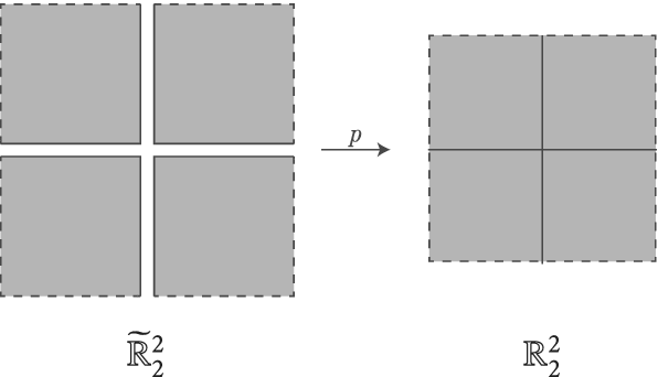
Figure 2: Boundaryfication of $\mathbb {R}^2$
with two coordinate axes.
$\mathbb {R}^2$
with two coordinate axes.
Notice that $p\colon \widetilde {\mathbb {R}}^n_{\ell } \to \mathbb {R}^n_{\ell }$
is a map of divisors, and if a smooth map
$p\colon \widetilde {\mathbb {R}}^n_{\ell } \to \mathbb {R}^n_{\ell }$
is a map of divisors, and if a smooth map $f\colon M \to \mathbb {R}^n$
has its image in a quadrant, then it admits a smooth lift to
$f\colon M \to \mathbb {R}^n$
has its image in a quadrant, then it admits a smooth lift to $\widetilde {\mathbb {R}}^n_{\ell }$
. Furthermore, if M is connected and the image of f has points which are not in the hyperplanes determined by
$\widetilde {\mathbb {R}}^n_{\ell }$
. Furthermore, if M is connected and the image of f has points which are not in the hyperplanes determined by $x_1 \cdots x_{\ell } = 0$
, then this lift is unique.
$x_1 \cdots x_{\ell } = 0$
, then this lift is unique.
For the global construction, we observe that charts in N provide a way to glue the local construction above to produce a manifold with corners. Indeed, given two charts that render the divisor in standard form, in their overlap, the change of coordinates gives a diffeomorphism $\Phi \colon \mathbb {R}^n_{\ell } \to \mathbb {R}^n_{\ell }$
, for some
$\Phi \colon \mathbb {R}^n_{\ell } \to \mathbb {R}^n_{\ell }$
, for some $\ell $
. Since the charts are adapted to the divisor,
$\ell $
. Since the charts are adapted to the divisor, $\Phi $
also induces a diffeomorphism of quadrants, that is, it lifts to a diffeomorphism
$\Phi $
also induces a diffeomorphism of quadrants, that is, it lifts to a diffeomorphism $\widetilde \Phi \colon (\widetilde {\mathbb {R}}^n_{\ell },\partial \widetilde {\mathbb {R}}^{n}_{\ell }) \to (\widetilde {\mathbb {R}}^n_{\ell }, \partial \widetilde {\mathbb {R}}^{n}_{\ell })$
.
$\widetilde \Phi \colon (\widetilde {\mathbb {R}}^n_{\ell },\partial \widetilde {\mathbb {R}}^{n}_{\ell }) \to (\widetilde {\mathbb {R}}^n_{\ell }, \partial \widetilde {\mathbb {R}}^{n}_{\ell })$
.
Since the changes of coordinates arising from an atlas for N give rise to a Čech cocycle of diffeomorphisms, the same holds for their lifts, so the procedure can be used to produce a manifold with corners $\widetilde {N}$
. Furthermore, the natural local maps, “p,” defined in coordinate charts above patch together to give a global map of divisors
$\widetilde {N}$
. Furthermore, the natural local maps, “p,” defined in coordinate charts above patch together to give a global map of divisors $p\colon (\widetilde N, \partial \widetilde N) \to (N,Z)$
. By construction,
$p\colon (\widetilde N, \partial \widetilde N) \to (N,Z)$
. By construction, $p\colon \widetilde N\backslash \partial \widetilde N \to N \backslash Z$
is a bijection away from the divisors and a local diffeomorphism onto its local image.
$p\colon \widetilde N\backslash \partial \widetilde N \to N \backslash Z$
is a bijection away from the divisors and a local diffeomorphism onto its local image.
Finally, if $p'\colon (N',\partial N') \to (N,Z)$
is a map of divisors with the two properties above, then we show that
$p'\colon (N',\partial N') \to (N,Z)$
is a map of divisors with the two properties above, then we show that $p'$
has a unique lift
$p'$
has a unique lift $\Psi \colon (N',\partial N') \to (\widetilde N,\partial \widetilde N) $
:
$\Psi \colon (N',\partial N') \to (\widetilde N,\partial \widetilde N) $
:

Indeed, in this case, $p^{-1} \circ p' \colon N'\backslash \partial N' \to \widetilde N \backslash \partial \widetilde N$
is a diffeomorphism and, by the third property, any point
$p^{-1} \circ p' \colon N'\backslash \partial N' \to \widetilde N \backslash \partial \widetilde N$
is a diffeomorphism and, by the third property, any point $x \in \partial N'$
has a connected neighborhood
$x \in \partial N'$
has a connected neighborhood $U \subset N'$
that maps diffeomorphically onto its image. Hence, taking U small enough, since U is connected,
$U \subset N'$
that maps diffeomorphically onto its image. Hence, taking U small enough, since U is connected, $p'(U)$
lies in a quadrant for a coordinate chart in N and hence
$p'(U)$
lies in a quadrant for a coordinate chart in N and hence $p'$
has a unique (local) lift to
$p'$
has a unique (local) lift to $\widetilde {N}$
. Patching these local lifts together, we obtain the map
$\widetilde {N}$
. Patching these local lifts together, we obtain the map $\Psi $
. Since
$\Psi $
. Since $\Psi $
is a diffeomorphism in the interior of
$\Psi $
is a diffeomorphism in the interior of $N'$
and by construction also a local diffeomorphism for points in the boundary of
$N'$
and by construction also a local diffeomorphism for points in the boundary of $N'$
, it is a global diffeomorphism.▪
$N'$
, it is a global diffeomorphism.▪
Definition 3.4 The boundarification of a manifold without boundary together with a real divisor, $(N,Z)$
, is a manifold with corners
$(N,Z)$
, is a manifold with corners $(\widetilde {N},\partial \widetilde N)$
together with a map
$(\widetilde {N},\partial \widetilde N)$
together with a map $p\colon (\widetilde N,\partial \widetilde N) \to (N,Z)$
satisfying the properties of Lemma 3.3.
$p\colon (\widetilde N,\partial \widetilde N) \to (N,Z)$
satisfying the properties of Lemma 3.3.
Example 3.5 If we take N to be the two-dimensional torus and Z to be an embedded circle which represents a primitive homology class, the boundarification of N is a cylinder and the map p identifies the two ends of the cylinder. If we take Z to be a pair of embedded circles intersecting transversely and which represent a basis for the homology of the torus, then the boundarification is a rectangle and the quotient map identifies opposite sides in the usual fashion.
Proposition 3.6 Let $f\colon (M,D)\to (N,Z)$
be a boundary map onto a manifold without boundary equipped with a real log divisor. Then there exists a unique boundary map
$f\colon (M,D)\to (N,Z)$
be a boundary map onto a manifold without boundary equipped with a real log divisor. Then there exists a unique boundary map $\widetilde {f} \colon (M,D)\to (\widetilde N,\partial \widetilde N)$
to its boundarification that is a lift of f, i.e., which satisfies
$\widetilde {f} \colon (M,D)\to (\widetilde N,\partial \widetilde N)$
to its boundarification that is a lift of f, i.e., which satisfies $f = p \circ \widetilde {f}$
for
$f = p \circ \widetilde {f}$
for $p \colon (\widetilde N, \partial \widetilde N) \to (N,Z)$
.
$p \colon (\widetilde N, \partial \widetilde N) \to (N,Z)$
.
Proof All we need to prove is that every point $x\in M$
has a neighborhood U such that
$x\in M$
has a neighborhood U such that $f|_U\colon U \to N$
admits a unique lift
$f|_U\colon U \to N$
admits a unique lift $\widetilde {f}|_U \colon U \to \widetilde {N}$
. Indeed, if this is the case, then any two such local lifts will agree in their overlap by uniqueness and hence the local lifts patch together to give a unique global map.
$\widetilde {f}|_U \colon U \to \widetilde {N}$
. Indeed, if this is the case, then any two such local lifts will agree in their overlap by uniqueness and hence the local lifts patch together to give a unique global map.
Since D has codimension 2 in M, every point $x \in M$
has a neighborhood U such that
$x \in M$
has a neighborhood U such that $U \backslash D$
is connected. It follows that
$U \backslash D$
is connected. It follows that $f(U \backslash D)$
lies in a connected component of
$f(U \backslash D)$
lies in a connected component of $N\backslash Z$
. By taking U small enough, we have that
$N\backslash Z$
. By taking U small enough, we have that $f(U\backslash D)$
lies in a connected component of the complement of Z in a coordinate patch
$f(U\backslash D)$
lies in a connected component of the complement of Z in a coordinate patch $V \subset N$
, that is,
$V \subset N$
, that is, $f(U \backslash D)$
lies in a quadrant and, by continuity, so does
$f(U \backslash D)$
lies in a quadrant and, by continuity, so does $f(U)$
. As such, there is a unique lift to a map
$f(U)$
. As such, there is a unique lift to a map $\widetilde f\colon U \to \widetilde {N}$
.▪
$\widetilde f\colon U \to \widetilde {N}$
.▪
We intend to use boundary maps to construct geometric structures on their total space. Thus, we can, without loss of generality, assume that the target of a boundary map is $(N,\partial N)$
, a manifold with corners whose real log divisor is determined by its boundary. This also explains the terminology “boundary map.”
$(N,\partial N)$
, a manifold with corners whose real log divisor is determined by its boundary. This also explains the terminology “boundary map.”
3.2 Boundary Lefschetz fibrations
The notion of a boundary map f is still too general to give us enough information about the singularities of the map. To get a good grasp on f, we need to ensure that its singularities are well controlled and this is what we do next. There are two ways to constrain the singularities of f: we can either impose that they display a specific behavior with respect to the ideals (and Lie algebroids) present, or we can impose that singularities disjoint from the vanishing loci of those ideals acquire a specific normal form. We will follow both routes here.
Note that a boundary map is by definition a map of pairs, so that it satisfies $f(D) \subseteq Z$
. The first restriction we impose is that the map moreover respects the stratifications present on both D and Z.
$f(D) \subseteq Z$
. The first restriction we impose is that the map moreover respects the stratifications present on both D and Z.
Definition 3.7 A fibrating boundary map is a boundary map $f\colon (M,D) \to (N,Z)$
such that, for each
$f\colon (M,D) \to (N,Z)$
such that, for each $k \geq 1$
, we have that:
$k \geq 1$
, we have that:
-
•
$f\colon (M,D[k]) \to (N,Z[k])$
is a strong map of pairs. -
• Each restriction
$\left .{f}\right |{}_{D[k]}\colon D[k] \rightarrow Z[k]$
is a submersion.


In Example 3.2, $f_1$
and
$f_1$
and $f_3$
are fibrating boundary maps, whereas
$f_3$
are fibrating boundary maps, whereas $f_2$
is not as it does not satisfy the first condition.
$f_2$
is not as it does not satisfy the first condition.
For a fibrating boundary map, f, we can use the ideals on M and N to control the singular behavior of f in a neighborhood of their corresponding divisors. Concretely, we have a pointwise normal form for the map.
Lemma 3.8 Let $f\colon (M^n,D^{n-2}) \rightarrow (N^m,Z^{m-1})$
be a fibrating boundary map, and let
$f\colon (M^n,D^{n-2}) \rightarrow (N^m,Z^{m-1})$
be a fibrating boundary map, and let $x \in D[k]$
. Then there exist coordinates
$x \in D[k]$
. Then there exist coordinates $(x_1,\ldots ,x_n)$
around x and
$(x_1,\ldots ,x_n)$
around x and $(z_1,\ldots ,z_k,y_i)$
around
$(z_1,\ldots ,z_k,y_i)$
around $f(x)$
such that:
$f(x)$
such that:
-
• Z is the standard log divisor with intersection number k on
$\mathbb {R}^k \times \mathbb {R}^{m-k}$
. -
• D is the standard elliptic divisor with intersection number k on
$\mathbb {R}^{2k}\times \mathbb {R}^{n-2k}$
. -
• In these coordinates, the map f takes the form
$$ \begin{align*} f(x_1,\ldots,x_n) = (x_1^2+x_2^2,\ldots,x_{2k-1}^2+x_{2k}^2,x_{n-m+k},\ldots,x_n). \end{align*} $$


Conversely, if for every point in D the map f is given in standard coordinates for the divisors by the expression above, then it is a fibrating boundary map.
Proof Choose a tubular neighbouhood $\mathcal {V}$
of
$\mathcal {V}$
of $Z[k]$
and denote by
$Z[k]$
and denote by $\text {pr}_{Z[k]}\colon NZ[k] \rightarrow Z[k]$
the projection. Let
$\text {pr}_{Z[k]}\colon NZ[k] \rightarrow Z[k]$
the projection. Let $V' \subset \mathcal {V}$
be an open neighborhood of
$V' \subset \mathcal {V}$
be an open neighborhood of $f(x)$
on which
$f(x)$
on which $Z[k]$
is the standard log divisor and write
$Z[k]$
is the standard log divisor and write $V'\cap Z[k] = \lbrace z_1\cdot \ldots \cdot z_k = 0 \rbrace $
. Choose a coordinate system
$V'\cap Z[k] = \lbrace z_1\cdot \ldots \cdot z_k = 0 \rbrace $
. Choose a coordinate system $(y_{k+1},\ldots ,y_m)$
on
$(y_{k+1},\ldots ,y_m)$
on $V' \cap Z[k]$
, so that the set
$V' \cap Z[k]$
, so that the set $\lbrace z_1,\ldots ,z_k,\text {pr}^*_{Z[k]} y_{k+1},\ldots ,\text {pr}^*_{Z[k]}y_m \rbrace $
forms a coordinate system on
$\lbrace z_1,\ldots ,z_k,\text {pr}^*_{Z[k]} y_{k+1},\ldots ,\text {pr}^*_{Z[k]}y_m \rbrace $
forms a coordinate system on $V'$
which is possible because
$V'$
which is possible because $\text {pr}_{Z[k]}$
is a submersion. Because f is a morphism of divisors,
$\text {pr}_{Z[k]}$
is a submersion. Because f is a morphism of divisors, $f^*(z_1 \cdot \ldots \cdot z_k)$
generates an elliptic divisor ideal on
$f^*(z_1 \cdot \ldots \cdot z_k)$
generates an elliptic divisor ideal on $U := f^{-1}(V') \subseteq M$
. Using that f is fibrating, after possibly shrinking U around x, let
$U := f^{-1}(V') \subseteq M$
. Using that f is fibrating, after possibly shrinking U around x, let $(x_1,\ldots ,x_n)$
be coordinates on U in which this is the standard elliptic divisor, and such that
$(x_1,\ldots ,x_n)$
be coordinates on U in which this is the standard elliptic divisor, and such that $f^*(z_j) = x_{2j-1}^2+x_{2j}^2$
. Because the restriction
$f^*(z_j) = x_{2j-1}^2+x_{2j}^2$
. Because the restriction $\left .{f}\right |{}_{Z[k]}$
is a submersion, we see that
$\left .{f}\right |{}_{Z[k]}$
is a submersion, we see that
 $$ \begin{align*} \lbrace x_1,\ldots,x_{2k},f^*\text{pr}^*_{Z[k]}y_{k+1},\ldots,f^*\text{pr}^*_{Z[k]}y_m \rbrace \end{align*} $$
forms a functionally independent set. We can complete this to a coordinate system on M and relabel these as $(x_1,\dots ,x_n)$
. If we use the coordinate system
$(x_1,\dots ,x_n)$
. If we use the coordinate system $(z_1,\ldots ,z_k,\text {pr}^*_{Z[k]}y_{k+1},\ldots ,\text {pr}^*_{Z[k]}y_m)$
on N and the above coordinates on M, then f takes the required form.
$(z_1,\ldots ,z_k,\text {pr}^*_{Z[k]}y_{k+1},\ldots ,\text {pr}^*_{Z[k]}y_m)$
on N and the above coordinates on M, then f takes the required form.
The converse follows immediately from the local expression for f.▪
Remark 3.9 Even if M and N are oriented manifolds and we require the use of coordinate charts compatible with orientations, we can still arrange that the local expression for f is given by the expression in Lemma 3.8. Indeed, using complex conjugation on the domain and permutation of the coordinates on both domain and codomain, we can change a coordinate chart which is not compatible with the given orientations into one that is.
In four dimensions, if $D[2]$
is nonempty, Lemma 3.8 implies that N is two-dimensional. Moreover, in a neighborhood of a point
$D[2]$
is nonempty, Lemma 3.8 implies that N is two-dimensional. Moreover, in a neighborhood of a point $p\in D[2]$
, orientations of M and N in fact dictate which one is “the first” strand of D arriving at p and which one is “the second,” as this information is determined by the orientation of N.
$p\in D[2]$
, orientations of M and N in fact dictate which one is “the first” strand of D arriving at p and which one is “the second,” as this information is determined by the orientation of N.
Lemma 3.10 Let $f\colon (M,D) \rightarrow (N,Z=\partial N)$
be a fibrating boundary map whose fibers near D are connected. Then the fibers of
$f\colon (M,D) \rightarrow (N,Z=\partial N)$
be a fibrating boundary map whose fibers near D are connected. Then the fibers of $\left .{f}\right |{}_{D[k]}\colon D[k] \rightarrow Z[k]$
are connected for all
$\left .{f}\right |{}_{D[k]}\colon D[k] \rightarrow Z[k]$
are connected for all $k\geq 1$
.
$k\geq 1$
.
Proof The proof goes by induction over the strata. Note that $Z[k+1]$
is a hypersurface in
$Z[k+1]$
is a hypersurface in $Z[k]$
, and therefore
$Z[k]$
, and therefore
 $$ \begin{align*} \left. {f} \right|_{D[k]} \colon (D[k],D[k+1]) \rightarrow (Z[k],Z[k+1]) \end{align*} $$
is a fibrating boundary map for all $k \geq 0$
. Applying [Reference Cavalcanti and Klaasse9, Proposition 5.25] to
$k \geq 0$
. Applying [Reference Cavalcanti and Klaasse9, Proposition 5.25] to $\left .{f}\right |{}_{M \backslash D(2)}$
tells us that the fibers of
$\left .{f}\right |{}_{M \backslash D(2)}$
tells us that the fibers of $\left .{f}\right |{}_{D[1]}$
are connected. Thus, we can apply the same result to
$\left .{f}\right |{}_{D[1]}$
are connected. Thus, we can apply the same result to $\left .{f}\right |{}_{D[1]}$
to conclude that the fibers of
$\left .{f}\right |{}_{D[1]}$
to conclude that the fibers of $\left .{f}\right |{}_{D[2]}$
are connected. Continuing inductively, we arrive at the desired result.▪
$\left .{f}\right |{}_{D[2]}$
are connected. Continuing inductively, we arrive at the desired result.▪
The conditions imposed on the maps have, up to this point, been on behavior near D. Next, we impose the conditions away from D:
Definition 3.11 A boundary fibration is a fibrating boundary map $f\colon (M,D) \to (N,Z)$
such that
$f\colon (M,D) \to (N,Z)$
such that $\left .{f}\right |{}_{M\backslash D}\colon M\backslash D \to N \backslash Z$
is a surjective submersion.
$\left .{f}\right |{}_{M\backslash D}\colon M\backslash D \to N \backslash Z$
is a surjective submersion.
Definition 3.12 A boundary Lefschetz fibration is a fibrating boundary map $f\colon (M^{2n},D) \to (\Sigma ^2,Z)$
between oriented manifolds such that
$f\colon (M^{2n},D) \to (\Sigma ^2,Z)$
between oriented manifolds such that $\left .{f}\right |{}_{M\backslash D}\colon M\backslash D \to \Sigma \backslash Z$
is a Lefschetz fibration. That is, the map
$\left .{f}\right |{}_{M\backslash D}\colon M\backslash D \to \Sigma \backslash Z$
is a Lefschetz fibration. That is, the map $f\colon M \to N$
is proper,
$f\colon M \to N$
is proper, $f|_{M\backslash D}$
is injective on critical points, and for each critical point
$f|_{M\backslash D}$
is injective on critical points, and for each critical point $p \in M\backslash D$
, there exist orientation-preserving complex coordinate charts centered at p and
$p \in M\backslash D$
, there exist orientation-preserving complex coordinate charts centered at p and $f(p)$
in which f takes the form
$f(p)$
in which f takes the form
 $$ \begin{align*} f\colon \mathbb{C}^n \to \mathbb{C}, \qquad f(z_1,\ldots,z_n) = z_1^2 + \cdots + z_n^2. \end{align*} $$
If M is four-dimensional, the definition above allows for three different types of singularities. These singularities have the following names (see also Section 6.4 for the relation with semitoric geometry).
Definition 3.13 Let $f\colon M^4 \to \Sigma ^2$
be a smooth map.
$f\colon M^4 \to \Sigma ^2$
be a smooth map.
-
• An elliptic singularity of f is a point p for which f has the local expression
$$ \begin{align*} f(x_1,x_2,x_3,x_4) = (x_1^2+x_2^2,x_4), \qquad x_i \in \mathbb{R}. \end{align*} $$
-
• An elliptic–elliptic singularity of f is a point p for which f has the local expression
$$ \begin{align*} f(x_1,x_2,x_3,x_4) = (x_1^2+x_2^2,x_3^2+x_4^2),\qquad x_i \in \mathbb{R}. \end{align*} $$
-
• A Lefschetz singularity of f is a point p for which f has the local expression
$$ \begin{align*}f(z_1,z_2) = z_1^2+z_2^2, \qquad z_i \in \mathbb{C}.\end{align*} $$


The level sets associated to these singularities are, respectively, an elliptic, elliptic–elliptic, and Lefschetz fiber.
For a boundary Lefschetz fibration $f : (M^4,D) \rightarrow (\Sigma ^2,Z)$
, the first two singularities above happen at the different strata of the divisor, whereas the Lefschetz singularities do not interact with the divisor. In dimension 4, the geometry of these fibrations can be understood.
$f : (M^4,D) \rightarrow (\Sigma ^2,Z)$
, the first two singularities above happen at the different strata of the divisor, whereas the Lefschetz singularities do not interact with the divisor. In dimension 4, the geometry of these fibrations can be understood.
Proposition 3.14 Let $f\colon (M^4,D^2) \rightarrow (\Sigma ^2,Z)$
be a boundary Lefschetz fibration with connected fibers, and let
$f\colon (M^4,D^2) \rightarrow (\Sigma ^2,Z)$
be a boundary Lefschetz fibration with connected fibers, and let $D'$
be a connected component of D. Then:
$D'$
be a connected component of D. Then:
-
• The regular fibers of f near D are tori.
-
• When
$D'[2]$
has
$k \geq 1$
points, then
$D'$
is a union of k pairwise transversely intersecting spheres.


In particular, if $D'[2] \neq \emptyset $
, then
$D'[2] \neq \emptyset $
, then $D'$
is co-orientable.
$D'$
is co-orientable.
Proof The first point follows immediately from [Reference Cavalcanti and Klaasse9, Corollary 5.18].
For the second, assume that $D'[2]$
has at least one point. Then
$D'[2]$
has at least one point. Then $\left .{f}\right |{}_{D[1]}\colon D[1] \rightarrow Z[1]$
is a surjective submersion by assumption, which by Lemma 3.10 has connected fibers. The corresponding locus
$\left .{f}\right |{}_{D[1]}\colon D[1] \rightarrow Z[1]$
is a surjective submersion by assumption, which by Lemma 3.10 has connected fibers. The corresponding locus $Z'[1]$
is a disjoint union of k open intervals, and as the fibers of
$Z'[1]$
is a disjoint union of k open intervals, and as the fibers of $\left .{f}\right |{}_{D[1]}$
are connected, they must be circles. Therefore,
$\left .{f}\right |{}_{D[1]}$
are connected, they must be circles. Therefore, $D'[1]$
has to be a disjoint union of cylinders. The immersed submanifold
$D'[1]$
has to be a disjoint union of cylinders. The immersed submanifold $D'$
is obtained from
$D'$
is obtained from $D'[1]$
by replacing the boundary circles by points and pairwise glueing these points, which implies it is as described above.
$D'[1]$
by replacing the boundary circles by points and pairwise glueing these points, which implies it is as described above.
Finally, because each component of $D'$
is an immersed sphere and thus automatically co-orientable, each component of
$D'$
is an immersed sphere and thus automatically co-orientable, each component of $D'[1]$
is also co-orientable.▪
$D'[1]$
is also co-orientable.▪
Therefore, to construct stable generalized complex structures using Corollary 2.27, the condition of co-orientability of D is satisfied as long as $D'[2]$
is nonempty for every component
$D'[2]$
is nonempty for every component $D'$
of D. For smooth components
$D'$
of D. For smooth components $D'$
of D, however, i.e., when
$D'$
of D, however, i.e., when $D'[2] = \emptyset $
, co-orientability is not guaranteed.
$D'[2] = \emptyset $
, co-orientability is not guaranteed.
3.3 Boundary maps and Lie algebroids
Given that the ideals $I_Z$
and
$I_Z$
and $I_{|D|}$
of a boundary map determine Lie algebroids, one should expect that boundary maps (and their further specializations) are compatible with them. This is indeed the case.
$I_{|D|}$
of a boundary map determine Lie algebroids, one should expect that boundary maps (and their further specializations) are compatible with them. This is indeed the case.
Lemma 3.15 Let $f\colon (M,D) \rightarrow (N,Z)$
be a boundary map. Then there is a Lie algebroid morphism
$f\colon (M,D) \rightarrow (N,Z)$
be a boundary map. Then there is a Lie algebroid morphism $(\varphi ,f)\colon \mathcal {A}_{\left | D \right |} \rightarrow \mathcal {A}_Z$
such that
$(\varphi ,f)\colon \mathcal {A}_{\left | D \right |} \rightarrow \mathcal {A}_Z$
such that $\varphi \equiv df$
on sections.
$\varphi \equiv df$
on sections.
Proof To prove that $df$
induces a Lie algebroid morphism
$df$
induces a Lie algebroid morphism $\varphi $
, by [Reference Cavalcanti and Klaasse9, Proposition 3.14], it suffices to show that
$\varphi $
, by [Reference Cavalcanti and Klaasse9, Proposition 3.14], it suffices to show that $f^*$
extends to an algebra morphism
$f^*$
extends to an algebra morphism $\varphi ^*\colon \Omega ^{\bullet }(\mathcal {A}_Z) \rightarrow \Omega ^{\bullet }(\mathcal {A}_{\left | D \right |})$
. This can be done locally, so given
$\varphi ^*\colon \Omega ^{\bullet }(\mathcal {A}_Z) \rightarrow \Omega ^{\bullet }(\mathcal {A}_{\left | D \right |})$
. This can be done locally, so given $p \in D$
and
$p \in D$
and $f(p) \in Z$
, consider coordinates adapted to the divisors as in Examples 2.6 and 2.9:
$f(p) \in Z$
, consider coordinates adapted to the divisors as in Examples 2.6 and 2.9:
 $$ \begin{align*} (X_1,Y_1,\ldots,X_s,Y_s,X_{2s+1},\ldots,X_n) \text{ around } p, \enspace (x_1,\ldots,x_j,y_{j+1},\ldots,y_{m}) \text{ around } f(p). \end{align*} $$
In these coordinates, we have
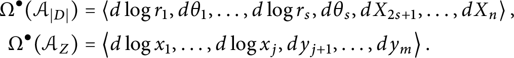 $$ \begin{align*} \Omega^{\bullet}(\mathcal{A}_{\left| D \right|}) &= \left\langle d\log r_1,d\theta_1,\ldots,d\log r_s,d\theta_s,dX_{2s+1},\ldots, dX_n \right\rangle,\\ \Omega^{\bullet}(\mathcal{A}_Z) &= \left\langle d\log x_1,\ldots,d\log x_j,dy_{j+1},\ldots,dy_m \right\rangle. \end{align*} $$
We must verify that $f^*(d \log x_i)$
defines an elliptic form. Because f is a morphism of divisors and the ideals are locally principal, it sends generators to generators; thus, there must exist a nowhere-vanishing function g such that
$f^*(d \log x_i)$
defines an elliptic form. Because f is a morphism of divisors and the ideals are locally principal, it sends generators to generators; thus, there must exist a nowhere-vanishing function g such that $f^*(x_1\cdot \ldots \cdot x_j) = gr_1^2\cdot \ldots \cdot r_s^2$
. Consequently, by functional indivisibility of the
$f^*(x_1\cdot \ldots \cdot x_j) = gr_1^2\cdot \ldots \cdot r_s^2$
. Consequently, by functional indivisibility of the $r_i^2$
, we conclude that
$r_i^2$
, we conclude that $f^*(x_i) = h r_{i_1}^2\cdot \ldots \cdot r_{i_{\ell }}^2$
for some nowhere vanishing function h and (possibly empty) subset
$f^*(x_i) = h r_{i_1}^2\cdot \ldots \cdot r_{i_{\ell }}^2$
for some nowhere vanishing function h and (possibly empty) subset $\{i_1,\ldots , i_{\ell }\} \subseteq \{1,\ldots ,s\}$
. We find that
$\{i_1,\ldots , i_{\ell }\} \subseteq \{1,\ldots ,s\}$
. We find that
 $$ \begin{align*} f^*(d\log x_i) = d\log f^*(x_i) = d\log h + 2d\log r_{i_1}+ \cdots +2d\log r_{i_l}, \end{align*} $$
which is an elliptic form as desired, so that $\varphi $
is a Lie algebroid morphism.
$\varphi $
is a Lie algebroid morphism.
The conditions imposed on boundary maps have a direct counterpart in Lie algebroid language. Given a Lie algebroid $\rho _{\mathcal {A}}\colon \mathcal {A} \to M$
, let
$\rho _{\mathcal {A}}\colon \mathcal {A} \to M$
, let $M_{\mathcal {A}}$
be the open subset where the anchor map is an isomorphism.
$M_{\mathcal {A}}$
be the open subset where the anchor map is an isomorphism.
Definition 3.16 [Reference Cavalcanti and Klaasse9]
A Lie algebroid morphism $(\varphi ,f)\colon (\mathcal {A},M) \to (\mathcal {A}',N)$
is said to be a:
$(\varphi ,f)\colon (\mathcal {A},M) \to (\mathcal {A}',N)$
is said to be a:
-
• Lie algebroid fibration if the induced morphism
$\varphi ^{!}\colon \mathcal {A} \to f^* \mathcal {A}'$
is surjective and -
• Lie algebroid Lefschetz fibration if
$M_{\mathcal {A}}$
is dense,
$f^{-1}(N_{\mathcal {A}'}) = M_{\mathcal {A}}$
, and there exists a discrete set
$\Delta \subset M_{\mathcal {A}}$
such that:-
–
$f|_{M_{\mathcal {A}}}\colon M_{\mathcal {A}} \to N_{\mathcal {A}'}$
is a Lefschetz fibration with
${\textrm {Crit}}(f|_{M_{\mathcal {A}}}) = \Delta $
and -
–
$(\varphi ,f)\colon (\mathcal {A}, M\backslash f^{-1}(f(\Delta ))) \to (\mathcal {A}',N\backslash f(\Delta ))$
is a Lie algebroid fibration.
Note that the Lefschetz condition forces that
${\textrm {rank}}(\mathcal {A}) = 2n$
and
${\textrm {rank}}(\mathcal {A}') = 2$
. -


The following lemmas follow immediately from the definition, combined with Lemma 3.15.
Lemma 3.17 Let $f\colon (M,D) \rightarrow (N,Z)$
be a boundary fibration. Then there is a Lie algebroid fibration
$f\colon (M,D) \rightarrow (N,Z)$
be a boundary fibration. Then there is a Lie algebroid fibration $(\varphi ,f)\colon (\mathcal {A}_{\left | D \right |},M) \rightarrow (\mathcal {A}_Z,N)$
such that
$(\varphi ,f)\colon (\mathcal {A}_{\left | D \right |},M) \rightarrow (\mathcal {A}_Z,N)$
such that $\varphi \equiv df$
on sections.
$\varphi \equiv df$
on sections.
Lemma 3.18 Let $f\colon (M^4,D^2) \rightarrow (N^2,Z^1)$
be a boundary Lefschetz fibration. Then there is a Lie algebroid Lefschetz fibration
$f\colon (M^4,D^2) \rightarrow (N^2,Z^1)$
be a boundary Lefschetz fibration. Then there is a Lie algebroid Lefschetz fibration $(\varphi ,f)\colon (\mathcal {A}_{\left | D \right |},M^4) \rightarrow (\mathcal {A}_Z,N^2)$
such that
$(\varphi ,f)\colon (\mathcal {A}_{\left | D \right |},M^4) \rightarrow (\mathcal {A}_Z,N^2)$
such that $\varphi \equiv df$
on sections.
$\varphi \equiv df$
on sections.
We summarize these statements and the relationship between the different concepts in the table below:
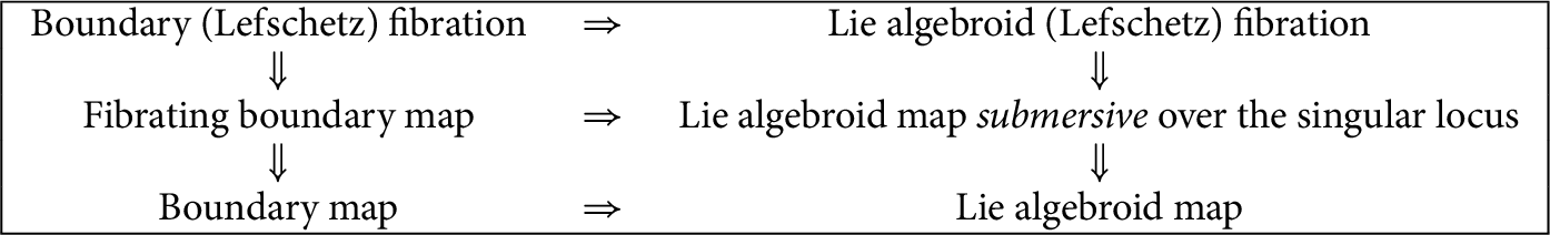
3.4 Construction of self-crossing stable generalized complex structures
With the desired notion of boundary Lefschetz fibration in hand, we are set to prove our first result relating them to stable generalized complex structures.
From now on, we will adopt the following convention: given a boundary Lefschetz fibration $f \colon (M,D) \to (N,Z)$
, we will orient the fibers of
$f \colon (M,D) \to (N,Z)$
, we will orient the fibers of $f\colon M\backslash D \to N\backslash Z$
by declaring that the orientation of the fiber together with the orientation of the base yield the orientation of M, so that each fiber determines a homology class on
$f\colon M\backslash D \to N\backslash Z$
by declaring that the orientation of the fiber together with the orientation of the base yield the orientation of M, so that each fiber determines a homology class on $M\backslash D$
. With this convention, integration over the fiber is a well-defined operation which induces the natural pairing between homology and cohomology.
$M\backslash D$
. With this convention, integration over the fiber is a well-defined operation which induces the natural pairing between homology and cohomology.
Definition 3.19 A surjective boundary Lefschetz fibration, $f\colon (M^4,D) \to (N^2,\partial N)$
, defined on a connected manifold M is homologically essential if the homology class
$f\colon (M^4,D) \to (N^2,\partial N)$
, defined on a connected manifold M is homologically essential if the homology class $[F]$
of a (and hence any) regular fiber of
$[F]$
of a (and hence any) regular fiber of $f\colon M \backslash D \rightarrow N \backslash Z$
is nontrivial in
$f\colon M \backslash D \rightarrow N \backslash Z$
is nontrivial in $H_2(M\backslash D;\mathbb {R})$
or, equivalently, if there is a class
$H_2(M\backslash D;\mathbb {R})$
or, equivalently, if there is a class $c \in H^2(M\backslash D;\mathbb {R})$
such that
$c \in H^2(M\backslash D;\mathbb {R})$
such that $\langle c,[F]\rangle \neq 0$
.
$\langle c,[F]\rangle \neq 0$
.
Definition 3.20 A boundary Lefschetz fibration, $f\colon (M^4,D) \to (N^2,Z)$
, and an elliptic symplectic form
$f\colon (M^4,D) \to (N^2,Z)$
, and an elliptic symplectic form $\omega \in \Omega ^2(\mathcal {A}_{|D|})$
are compatible if
$\omega \in \Omega ^2(\mathcal {A}_{|D|})$
are compatible if $\ker \varphi \subseteq \mathcal {A}_{|D|}$
consists of symplectic vector spaces, where
$\ker \varphi \subseteq \mathcal {A}_{|D|}$
consists of symplectic vector spaces, where $\varphi \colon \mathcal {A}_{|D|} \to \mathcal {A}_Z$
is the induced map of Lie algebroids.
$\varphi \colon \mathcal {A}_{|D|} \to \mathcal {A}_Z$
is the induced map of Lie algebroids.
In what follows, we will have two ongoing simplifying assumptions:
-
(1) We will assume that the target manifold is
$(N,\partial N)$
. This is not a restriction since by Proposition 3.6 we can lift f to a boundary Lefschetz fibration over the boundaryfication of
$(N,Z)$
. -
(2) We will assume that the level sets of f are connected. This also is not restriction since by [Reference Cavalcanti and Klaasse9, Proposition 5.24] we may assume that the generic fibers of f are connected and Lemma 3.10 then implies that the level sets over
$Z[1]$
and
$Z[2]$
are connected as well.


Before we continue, it is worth to stop and take stock of where we stand and place our quest into context. The case when the elliptic divisor is smooth was already treated in [Reference Cavalcanti and Klaasse9]. Even though there the authors only dealt with the compact case, the following is an immediate generalization for a proper map.
Theorem 3.21 [Reference Cavalcanti and Klaasse9, Theorem 7.1]
Let $(M^4,I_{|D|})$
be an oriented manifold with a smooth elliptic divisor, and let
$(M^4,I_{|D|})$
be an oriented manifold with a smooth elliptic divisor, and let $f\colon (M,D) \rightarrow (N^2,Z,\omega _{N})$
be a homologically essential, proper, Lefschetz fibration with connected fibers over a possibly open log-symplectic surface. Denote by
$f\colon (M,D) \rightarrow (N^2,Z,\omega _{N})$
be a homologically essential, proper, Lefschetz fibration with connected fibers over a possibly open log-symplectic surface. Denote by $\varphi \colon \mathcal {A}_{|D|} \to \mathcal {A}_Z$
the induced map of Lie algebroids. Let
$\varphi \colon \mathcal {A}_{|D|} \to \mathcal {A}_Z$
the induced map of Lie algebroids. Let $c \in H^2(M\backslash D) = H^2_{0,0}(M,\mathcal {A}_{|D|})$
be a cohomology class such that
$c \in H^2(M\backslash D) = H^2_{0,0}(M,\mathcal {A}_{|D|})$
be a cohomology class such that $\langle c, [F]\rangle> 0$
, where F is a regular fiber of f. Then there exists a closed two-form
$\langle c, [F]\rangle> 0$
, where F is a regular fiber of f. Then there exists a closed two-form $\eta \in \Omega ^2_{0,0}(M,\mathcal {A}_{|D|})$
with
$\eta \in \Omega ^2_{0,0}(M,\mathcal {A}_{|D|})$
with $[\eta ] =c$
and a positive function
$[\eta ] =c$
and a positive function $\rho _0 \in C^{\infty }(N)$
such that:
$\rho _0 \in C^{\infty }(N)$
such that:
-
•
$\eta $
is fiberwise nondegenerate, that is, for every
$p \in M$
,
$\eta $
is nondegenerate in
$\mathrm {ker}(\varphi _p)$
. -
• The form
$\omega = \eta + f^*(\rho \omega _{\Sigma })$
is symplectic with zero elliptic residue on
$\mathcal {A}_{|D|}$
for every
$\rho \in C^{\infty } (N)$
as long as
$\rho \geq \rho _0$
.


Apart from the theorem above, [Reference Cavalcanti and Klaasse9] also includes a general Gompf–Thurston result for Lie algebroid Lefschetz fibrations: under similar conditions on a Lie algebroid Lefschetz fibration, one can construct a Lie algebroid symplectic form on the domain by adding a form which is symplectic on the fibers to a large multiple of the pull back of a symplectic form on the base.
Neither result can be directly applied to our case: Theorem 3.21 does not work because our divisor is not smooth, while the failure of the general result on Lie algebroid fibrations to yield stable generalized complex structures can already be seen in the simplest example.
Example 3.22 Consider the boundary fibration:
 $$ \begin{align*} f_1\colon (\mathbb{C}^2, D) \to (\mathbb{R}^2,Z), \qquad f_1(z_1,z_2) = (|z_1|^2,|z_2|^2), \end{align*} $$
where D and Z are the coordinate axes on $\mathbb {C}^2$
and
$\mathbb {C}^2$
and $\mathbb {R}^2$
, respectively, as in Example 3.2.
$\mathbb {R}^2$
, respectively, as in Example 3.2.
We can endow $\mathbb {R}^2$
with the log-symplectic structure
$\mathbb {R}^2$
with the log-symplectic structure $d\log x_1 \wedge d\log x_2$
, and consider on
$d\log x_1 \wedge d\log x_2$
, and consider on $\mathbb {C}^2$
the closed elliptic form
$\mathbb {C}^2$
the closed elliptic form
 $$ \begin{align*}\eta = -d\theta_1 \wedge d\theta_2 + d\log r_1 \wedge d \theta_2 + d\log r_2 \wedge d\theta_1, \end{align*} $$
which is nondegenerate on the fibers of $f_1$
. The Gompf–Thurston theorem then provides us with a one-parameter family of forms
$f_1$
. The Gompf–Thurston theorem then provides us with a one-parameter family of forms
 $$ \begin{align*} \omega_t = \eta+ tf_1^*(d\log x_1 \wedge d\log x_2), \end{align*} $$
which is elliptic symplectic for $t>1$
. This poses a problem: although this defines a legitimate elliptic symplectic form, there is no value of t for which it corresponds to a stable generalized complex structure, since
$t>1$
. This poses a problem: although this defines a legitimate elliptic symplectic form, there is no value of t for which it corresponds to a stable generalized complex structure, since $\left | \operatorname {\mathrm {Res}}_{r_1r_2}\omega _t \right | \neq \left | \operatorname {\mathrm {Res}}_{\theta _1\theta _2}\omega _t \right |$
for
$\left | \operatorname {\mathrm {Res}}_{r_1r_2}\omega _t \right | \neq \left | \operatorname {\mathrm {Res}}_{\theta _1\theta _2}\omega _t \right |$
for $t>1$
. We conclude that the process of scaling up the log-symplectic structure on the base to achieve nondegeneracy is incompatible with the residue conditions.
$t>1$
. We conclude that the process of scaling up the log-symplectic structure on the base to achieve nondegeneracy is incompatible with the residue conditions.
What we do next is to adapt Theorem 3.21 for the self-crossing case.
Theorem 3.23 Let $f\colon (M^4,D^2)\to (N^2,Z=\partial N)$
be a homologically essential boundary Lefschetz fibration with connected fibers between compact connected oriented manifolds. Denote by
$f\colon (M^4,D^2)\to (N^2,Z=\partial N)$
be a homologically essential boundary Lefschetz fibration with connected fibers between compact connected oriented manifolds. Denote by $\varphi \colon \mathcal {A}_{|D|} \to \mathcal {A}_Z$
the induced map of Lie algebroids. Then
$\varphi \colon \mathcal {A}_{|D|} \to \mathcal {A}_Z$
the induced map of Lie algebroids. Then $(M,I_{|D|})$
admits an elliptic symplectic structure with zero elliptic residue and imaginary parameter which is compatible with f.
$(M,I_{|D|})$
admits an elliptic symplectic structure with zero elliptic residue and imaginary parameter which is compatible with f.
If D is co-orientable and the index of each connected component of D is $1$
, this elliptic symplectic structure induces a stable generalized complex structure.
$1$
, this elliptic symplectic structure induces a stable generalized complex structure.
Proof Fix a log-symplectic structure $\omega _N \in \Omega ^2(N,\mathcal {A}_{Z})$
. First, we consider
$\omega _N \in \Omega ^2(N,\mathcal {A}_{Z})$
. First, we consider $f\colon M\backslash D[2] \to N\backslash Z[2]$
. This is a homologically essential, proper, boundary Lefschetz fibration with smooth elliptic divisor; hence, by Theorem 3.21, there is a form
$f\colon M\backslash D[2] \to N\backslash Z[2]$
. This is a homologically essential, proper, boundary Lefschetz fibration with smooth elliptic divisor; hence, by Theorem 3.21, there is a form $\eta \in \Omega _{0,0}^2(M\backslash D[2];\log |D\backslash D[2]|)$
and a function
$\eta \in \Omega _{0,0}^2(M\backslash D[2];\log |D\backslash D[2]|)$
and a function $\rho _0 \in \Omega ^0(N \backslash Z[2])$
(recall Definition 2.14) such that
$\rho _0 \in \Omega ^0(N \backslash Z[2])$
(recall Definition 2.14) such that $\omega = \eta + f^*( \rho \omega _N)$
is a zero elliptic residue symplectic form for any function
$\omega = \eta + f^*( \rho \omega _N)$
is a zero elliptic residue symplectic form for any function $\rho \in \Omega ^0(N\backslash Z[2])$
with
$\rho \in \Omega ^0(N\backslash Z[2])$
with $\rho \geq \rho _0$
.
$\rho \geq \rho _0$
.
Now, we show how to change this construction, so that the form it yields extends over $D[2]$
, is elliptic symplectic with zero elliptic residue, and has imaginary parameter.
$D[2]$
, is elliptic symplectic with zero elliptic residue, and has imaginary parameter.
For each point $p \in D[2]$
, fix open neighborhoods
$p \in D[2]$
, fix open neighborhoods $U_1 \Subset U_2 \Subset U_3$
and oriented coordinates charts defined on
$U_1 \Subset U_2 \Subset U_3$
and oriented coordinates charts defined on $U_3$
and
$U_3$
and $f(U_3)$
in which f has the form
$f(U_3)$
in which f has the form
 $$ \begin{align*}f(z_1,z_2) = (|z_1|^2, |z_2|^2). \end{align*} $$
As usual, we express the complex coordinates in $U_3$
in polar form,
$U_3$
in polar form, $z_i = r_i e^{i \theta _i}$
, and denote by
$z_i = r_i e^{i \theta _i}$
, and denote by $(x_1,x_2)$
the coordinates on the base, so
$(x_1,x_2)$
the coordinates on the base, so $f^*x_i = r_i^2$
.
$f^*x_i = r_i^2$
.
The strategy will be to change the symplectic form $\omega $
described above in a very precise way:
$\omega $
described above in a very precise way:
-
• In the complement of
$U_3$
,
$\omega $
remains unchanged except for a further constant scaling of the symplectic form
$\omega _N$
. -
• In
$U_3\backslash U_2$
, we change
$\eta $
into a multiple of
$d\theta _2 \wedge d\theta _1$
and we preserve nondegeneracy by rescaling the symplectic form
$\omega _N$
by a constant. -
• In
$U_2\backslash U_1$
, we interpolate the possibly large
$f^*\omega _N$
to
$f^*(d\log x_1 \wedge d\log x_2)$
and observe that this interpolation does not spoil the symplectic condition. -
• In
$U_1$
, we extend the symplectic form as
$d\theta _2 \wedge d\theta _1 + d\log r_1 \wedge d\log r_2$
, which clearly has the desired properties at p.


Now, we carry out his plan explicitly. Fix $\rho \geq \rho _0$
. On
$\rho \geq \rho _0$
. On $U_3$
, we have by Lemma 2.15 that
$U_3$
, we have by Lemma 2.15 that
 $$ \begin{align*} [\eta] \in H^2_{0,0}(U_3\backslash D[2],\mathcal{A}_{|D\backslash D[2]|}) \cong H^2(U_3\backslash D) =\mathbb{R}, \end{align*} $$
and the generator of this cohomology pairs nonzero with the torus given in coordinates by $F = f^{-1}(r_1,r_2)$
, where
$F = f^{-1}(r_1,r_2)$
, where $r_1$
and
$r_1$
and $r_2$
are any two small positive numbers. Let
$r_2$
are any two small positive numbers. Let $\lambda = \int _F \eta $
where integration is with respect to the fiber orientation of F, and hence
$\lambda = \int _F \eta $
where integration is with respect to the fiber orientation of F, and hence $\lambda>0$
. On
$\lambda>0$
. On $U_3$
, consider the elliptic form
$U_3$
, consider the elliptic form $\widetilde \eta = \frac {\lambda }{4\pi ^2}d\theta _2 \wedge d\theta _1$
. Then
$\widetilde \eta = \frac {\lambda }{4\pi ^2}d\theta _2 \wedge d\theta _1$
. Then $\widetilde \eta $
is closed in
$\widetilde \eta $
is closed in $U_3$
and also integrates to
$U_3$
and also integrates to $\lambda $
over F. Therefore,
$\lambda $
over F. Therefore, $[\eta ] =[\widetilde \eta ] \in H^2(U_3\backslash \{p\},\mathcal {A}_{D\backslash \{p\}})$
, and there is a one-form
$[\eta ] =[\widetilde \eta ] \in H^2(U_3\backslash \{p\},\mathcal {A}_{D\backslash \{p\}})$
, and there is a one-form $\alpha \in \Omega ^1(U_3\backslash \{p\}, \mathcal {A}_{|D\backslash \{p\}|})$
such that
$\alpha \in \Omega ^1(U_3\backslash \{p\}, \mathcal {A}_{|D\backslash \{p\}|})$
such that $\widetilde \eta = \eta + d\alpha $
.
$\widetilde \eta = \eta + d\alpha $
.
Let $k\geq 1$
, and let
$k\geq 1$
, and let $\psi _1$
and
$\psi _1$
and $\psi _2$
be positive functions on
$\psi _2$
be positive functions on $f(U_3)$
such that
$f(U_3)$
such that $\psi _1$
is equal to
$\psi _1$
is equal to $1$
in neighborhood of
$1$
in neighborhood of $f(U_1)$
and has support in
$f(U_1)$
and has support in $f(U_2)$
and
$f(U_2)$
and $\psi _2$
is equal to
$\psi _2$
is equal to $1$
in neighborhood of
$1$
in neighborhood of $f(U_2)$
and has support in
$f(U_2)$
and has support in $f(U_3)$
. Then consider the form
$f(U_3)$
. Then consider the form
 $$ \begin{align*}\widetilde\omega := \begin{cases} \frac{\lambda}{4\pi^2}(d\theta_2 \wedge d\theta_1 + d\log r_1 \wedge d\log r_2) & \mbox{ in } U_1,\\ \widetilde\eta + f^*((1-\psi_1) k\rho \omega_N + \psi_1\frac{\lambda}{4\pi^2}d\log x_1 \wedge d\log x_2)& \mbox{ in } U_2\backslash U_1,\\ \eta + d ((f^*\psi_2)\alpha) + f^*(k\rho \omega_N)& \mbox{ in } U_3\backslash U_2,\\ \eta + f^*(k\rho \omega_N)& \mbox{ in } M\backslash U_3. \end{cases} \end{align*} $$
Because of our choice of bump functions, this form is smooth. Moreover, it is clearly closed. Since $k\geq 1$
, we have
$k\geq 1$
, we have $k\rho \geq \rho \geq \rho _0$
, and hence
$k\rho \geq \rho \geq \rho _0$
, and hence $\widetilde \omega $
is symplectic in
$\widetilde \omega $
is symplectic in $M\backslash U_3$
for all possible values of k.
$M\backslash U_3$
for all possible values of k.
On $\overline {U_3\backslash U_2}$
, we observe that the form
$\overline {U_3\backslash U_2}$
, we observe that the form $\eta + d ((f^*\psi )\alpha )$
is fiberwise symplectic. Indeed, its restriction to each fiber is given by
$\eta + d ((f^*\psi )\alpha )$
is fiberwise symplectic. Indeed, its restriction to each fiber is given by
 $$ \begin{align*} \eta + (f^*\psi_2) d\alpha = (f^*\psi_2)(\eta + d\alpha) + (1-(f^*\psi_2))\eta = (f^*\psi_2)\widetilde\eta + (1-(f^*\psi_2))\eta; \end{align*} $$
hence, it is a convex combination of $\eta $
and
$\eta $
and $\widetilde \eta $
, and these are both symplectic and determine the same orientation on each fiber. Since
$\widetilde \eta $
, and these are both symplectic and determine the same orientation on each fiber. Since $\eta + d ((f^*\psi )\alpha )$
is fiberwise symplectic and
$\eta + d ((f^*\psi )\alpha )$
is fiberwise symplectic and $\rho \omega _N$
is symplectic on N, the combination
$\rho \omega _N$
is symplectic on N, the combination $\eta + d ((f^*\psi )\alpha ) + f^*(k\rho \omega _N)$
is symplectic on the compact set
$\eta + d ((f^*\psi )\alpha ) + f^*(k\rho \omega _N)$
is symplectic on the compact set $\overline {U_3\backslash U_2}$
as long as k is large enough.
$\overline {U_3\backslash U_2}$
as long as k is large enough.
On $U_2 \backslash U_1$
, the form
$U_2 \backslash U_1$
, the form $\widetilde \eta $
is given by
$\widetilde \eta $
is given by $\frac {\lambda }{4\pi ^2} d\theta _2 \wedge d\theta _1$
, while the summand
$\frac {\lambda }{4\pi ^2} d\theta _2 \wedge d\theta _1$
, while the summand $f^*((1-\psi _1) k\rho \omega _N + \psi _1d\log x_1 \wedge d\log x_2)$
is a convex combination of two log-symplectic structures on N which determine the same orientation, that is,
$f^*((1-\psi _1) k\rho \omega _N + \psi _1d\log x_1 \wedge d\log x_2)$
is a convex combination of two log-symplectic structures on N which determine the same orientation, that is,
 $$ \begin{align*} f^*((1-\psi_1) k\rho \omega_N + \psi_1\frac{\lambda}{4\pi^2} d\log x_1 \wedge d\log x_2) = f^*(\kappa d\log x_1 \wedge d\log x_2), \end{align*} $$
for some positive function $\kappa $
, and hence, on
$\kappa $
, and hence, on $U_2 \backslash U_1$
,
$U_2 \backslash U_1$
,
 $$ \begin{align*} \widetilde\omega= \frac{\lambda}{4\pi^2} d\theta_2 \wedge d\theta_1 + (f^*\kappa) d\log r_1 \wedge d\log r_2, \end{align*} $$
which is clearly (zero residue) elliptic symplectic.
Finally, on $U_1$
, we have
$U_1$
, we have $\omega = \mathrm {Im}(i \frac {\lambda }{4\pi ^2}d\log z_1 \wedge d\log z_2)$
, showing that it has the desired properties.▪
$\omega = \mathrm {Im}(i \frac {\lambda }{4\pi ^2}d\log z_1 \wedge d\log z_2)$
, showing that it has the desired properties.▪
4 Connected sums of boundary Lefschetz fibrations
In this section, we describe a connected sum procedure for boundary Lefschetz fibrations along zero-dimensional strata of their elliptic divisors. This procedure will allow us to construct elaborate examples out of basic ones. For simplicity, we immediately restrict ourselves to dimension 4, but we note that since the connected sum takes place at points of the divisor, this procedure can also be carried out for boundary fibrations in higher dimensions.
Before we start taking connected sums of boundary Lefschetz fibrations, first recall from [Reference Cavalcanti, Klaasse and Witte11, Lemma 6.1] that we can take connected sums of elliptic divisors.
Lemma 4.1 Let $M_1^4,M_2^4$
be oriented manifolds endowed with elliptic divisors
$M_1^4,M_2^4$
be oriented manifolds endowed with elliptic divisors $I_{\left | D_1 \right |},I_{\left | D_2 \right |}$
, respectively, and let
$I_{\left | D_1 \right |},I_{\left | D_2 \right |}$
, respectively, and let $p_i \in D_i[2]$
. Then
$p_i \in D_i[2]$
. Then $M_1 \#_{p_1,p_2} M_2$
admits an elliptic divisor
$M_1 \#_{p_1,p_2} M_2$
admits an elliptic divisor $I_{\left | \widetilde {D} \right |}$
for which the natural inclusions
$I_{\left | \widetilde {D} \right |}$
for which the natural inclusions $(M\backslash \lbrace p_i \rbrace ,I_{\left | D_i \right |}) \rightarrow (M_1\#_{p_1,p_2} M_2,I_{\left | \widetilde {D} \right |})$
are morphisms of divisors.
$(M\backslash \lbrace p_i \rbrace ,I_{\left | D_i \right |}) \rightarrow (M_1\#_{p_1,p_2} M_2,I_{\left | \widetilde {D} \right |})$
are morphisms of divisors.
Similarly, recall from [Reference Cavalcanti, Klaasse and Witte11, Lemma 6.1] that we can perform a self-connected sum, which when M is connected corresponds to attaching a 1-handle, and hence the diffeomorphism type of the resulting space is $M \#(S^1\times S^3)$
.
$M \#(S^1\times S^3)$
.
Lemma 4.2 Let $M^4$
be an oriented connected manifold endowed with an elliptic divisor
$M^4$
be an oriented connected manifold endowed with an elliptic divisor $I_{\left | D \right |}$
, and let
$I_{\left | D \right |}$
, and let $p_1,p_2 \in D[2]$
be distinct points. Then
$p_1,p_2 \in D[2]$
be distinct points. Then $M \#(S^1\times S^3)$
and admits an elliptic divisor
$M \#(S^1\times S^3)$
and admits an elliptic divisor $I_{\left | \widetilde {D} \right |}$
for which the natural inclusion
$I_{\left | \widetilde {D} \right |}$
for which the natural inclusion $(M\backslash \lbrace p_1,p_2 \rbrace ,I_{\left | D \right |}) \rightarrow (M\#(S^1 \times S^3),I_{\left | \widetilde {D} \right |})$
is a morphism of divisors.
$(M\backslash \lbrace p_1,p_2 \rbrace ,I_{\left | D \right |}) \rightarrow (M\#(S^1 \times S^3),I_{\left | \widetilde {D} \right |})$
is a morphism of divisors.
In this connected sum procedure, the map $\Phi (z_1,z_2) = \frac {1}{\left | z_1 \right |{}^2+\left | z_2 \right |{}^2}(z_2,\overline {z}_1)$
is used to identify annuli. Here,
$\Phi (z_1,z_2) = \frac {1}{\left | z_1 \right |{}^2+\left | z_2 \right |{}^2}(z_2,\overline {z}_1)$
is used to identify annuli. Here, $(z_1,z_2)$
are local complex coordinates compatible with the orientation on the manifolds. There is some freedom in the constructions above. Given a choice of local coordinates
$(z_1,z_2)$
are local complex coordinates compatible with the orientation on the manifolds. There is some freedom in the constructions above. Given a choice of local coordinates $(z_1,z_2)$
around
$(z_1,z_2)$
around $p_1$
and
$p_1$
and $p_2$
, we can compose the map
$p_2$
, we can compose the map $\Phi $
by a permutation of the coordinates. This does not change the topology of
$\Phi $
by a permutation of the coordinates. This does not change the topology of $M_1 \#_{p_1,p_2} M_2$
, but it could change the topology of the zero locus of the divisor. In dimension 4, because of this freedom in the ordering, there are potentially two different topological types of the zero locus of the divisor. Notice, however, that our notation does not reflect this ambiguity.
$M_1 \#_{p_1,p_2} M_2$
, but it could change the topology of the zero locus of the divisor. In dimension 4, because of this freedom in the ordering, there are potentially two different topological types of the zero locus of the divisor. Notice, however, that our notation does not reflect this ambiguity.
Remark 4.3 (Connected components)
Although there is some freedom in the choices, we can still distinguish the number of connected components on the divisor on the connected sum:
-
(1) When
$p_1$
and
$p_2$
lie in different connected components of the divisor, be that either in the connected sum of two manifolds or in a self-connected sum, the connected components containing
$p_1$
and
$p_2$
will combine into a single connected component of
$\widetilde {D}$
. -
(2) When
$p_1$
and
$p_2$
are in the same connected component, D, a case that can only happen in a self-connected sum, the resulting divisor,
$\widetilde {D} \subset M\#(S^1\times S^3)$
, may have one or two connected components originating from D.


Next, we show that the connected sum operation is also compatible with boundary (Lefschetz) fibrations. To describe how the connected sum procedure interacts with the base of the fibration, we first consider what happens in the local model.
Lemma 4.4 Let $\Delta _r \subseteq \mathbb {R}^2$
be the triangle bounded by the axes and the line
$\Delta _r \subseteq \mathbb {R}^2$
be the triangle bounded by the axes and the line $x + y = r$
, and let
$x + y = r$
, and let $(x,y)$
be oriented coordinates on
$(x,y)$
be oriented coordinates on $\Delta _r$
and
$\Delta _r$
and $(z_1,z_2)$
be complex coordinates on
$(z_1,z_2)$
be complex coordinates on $\mathbb {D}^4_r$
, the disk of radius r. Consider the following maps:
$\mathbb {D}^4_r$
, the disk of radius r. Consider the following maps:
-
•
$p\colon (\mathbb {D}^{4}_2\backslash \mathbb {D}^4_{1/2}) \to (\Delta _2\backslash \Delta _{1/2})$
, given by
$(z_1,z_2) \mapsto (\left | z_1 \right |{}^2,\left | z_2 \right |{}^2)$
. -
•
$\Phi \colon (\mathbb {D}^{4}_2\backslash \mathbb {D}^4_{1/2}) \rightarrow (\mathbb {D}^{4}_2\backslash \mathbb {D}^4_{1/2})$
, given by
$(z_1,z_2) \mapsto \frac {1}{\left | z_1 \right |{}^2+\left | z_2 \right |{}^2}(z_2,\overline {z}_1)$
. -
•
$\Psi \colon (\Delta _2\backslash \Delta _{1/2}) \rightarrow (\Delta _2\backslash \Delta _{1/2})$
given by
$(x,y) \mapsto \frac {(y,x)}{(x+y)^2}$
.


Then the following diagram commutes:

The proof of this lemma is a simple verification. Just as we used the map $\Phi $
to perform a connected sum compatible with elliptic divisors, we want to use the map
$\Phi $
to perform a connected sum compatible with elliptic divisors, we want to use the map $\Psi $
to define a sort of connected sum operation of the base.
$\Psi $
to define a sort of connected sum operation of the base.
Definition 4.5 Let $\Sigma _1,\Sigma _2$
be oriented surfaces with corners, and let
$\Sigma _1,\Sigma _2$
be oriented surfaces with corners, and let $q_1,q_2$
be corners of
$q_1,q_2$
be corners of $\Sigma _1,\Sigma _2$
, respectively. The oriented corner connected sum of
$\Sigma _1,\Sigma _2$
, respectively. The oriented corner connected sum of $\Sigma _1$
and
$\Sigma _1$
and $\Sigma _2$
is defined by identifying a trapezoid neighborhood of
$\Sigma _2$
is defined by identifying a trapezoid neighborhood of $q_1$
to a trapezoid neighborhood of
$q_1$
to a trapezoid neighborhood of $q_2$
via
$q_2$
via $\Psi $
. The oriented corner connected sum is an oriented surface with corners denoted by
$\Psi $
. The oriented corner connected sum is an oriented surface with corners denoted by $\Sigma _1 \#_{q_1,q_2} \Sigma _2$
(see Figure 3).
$\Sigma _1 \#_{q_1,q_2} \Sigma _2$
(see Figure 3).

Figure 3: Local oriented and orientation-reversing corner connected sums.
The oriented corner connected sum is naturally oriented and does not depend on the neighborhoods chosen. Together with the local normal form for fibrating boundary maps, we can now prove the following.
Theorem 4.6 Let $f_i\colon (M_i^4,D_i) \rightarrow (N_i^2,\partial N_i)$
be boundary (Lefschetz) fibrations with connected fibers between oriented manifolds for
$f_i\colon (M_i^4,D_i) \rightarrow (N_i^2,\partial N_i)$
be boundary (Lefschetz) fibrations with connected fibers between oriented manifolds for $i=1,2$
, let
$i=1,2$
, let $p_i \in D_i[2]$
and
$p_i \in D_i[2]$
and $q_i = f(p_i)$
. Then there exists a boundary (Lefschetz) fibration on one of the two possible connected sums
$q_i = f(p_i)$
. Then there exists a boundary (Lefschetz) fibration on one of the two possible connected sums $M_1 \#_{p_1,p_2} M_2$
whose base is the oriented corner sum
$M_1 \#_{p_1,p_2} M_2$
whose base is the oriented corner sum $N_1 \#_{q_1,q_2}N_2$
:
$N_1 \#_{q_1,q_2}N_2$
:
 $$ \begin{align*} (f_1 \# f_2)\colon (M_1 \#_{p_1,p_2} M_2,\widetilde{D}) \rightarrow (N_1 \#_{f(p_1),f(p_2)} N_2,\partial N_1\#_{q_1,q_2} \partial N_2), \end{align*} $$
which is compatible with the (orientation-preserving) inclusions $M_i \backslash \lbrace p_i \rbrace \hookrightarrow M_1\#M_2$
.
$M_i \backslash \lbrace p_i \rbrace \hookrightarrow M_1\#M_2$
.
Furthermore, let $D_1',D_2'$
denote the connected components of the zero locus of the divisor D containing
$D_1',D_2'$
denote the connected components of the zero locus of the divisor D containing $p_1,p_2$
, respectively. Then the parities satisfy:
$p_1,p_2$
, respectively. Then the parities satisfy:
 $$ \begin{align*} \varepsilon_{\widetilde{D}} = -\varepsilon_{D_1'}\varepsilon_{D_2'}. \end{align*} $$
Finally, $f_1 \# f_2$
is homologically essential if and only if
$f_1 \# f_2$
is homologically essential if and only if $f_1$
and
$f_1$
and $f_2$
are.
$f_2$
are.
Proof By Lemma 3.8, there exist neighborhoods $U_1$
,
$U_1$
, $U_2$
of
$U_2$
of $f(p_1)$
,
$f(p_1)$
, $f(p_2)$
, respectively, which provide coordinates as in the setting of Lemma 4.4. We perform the connected sum procedure using the maps described there. Because these maps are compatible with the fibrations on
$f(p_2)$
, respectively, which provide coordinates as in the setting of Lemma 4.4. We perform the connected sum procedure using the maps described there. Because these maps are compatible with the fibrations on $M_1$
and
$M_1$
and $M_2$
, we conclude that
$M_2$
, we conclude that $M_1 \#_{p_1,p_2} M_2$
admits a boundary fibration. The computation of the parity is given in [Reference Cavalcanti, Klaasse and Witte11, Theorem 6.7].▪
$M_1 \#_{p_1,p_2} M_2$
admits a boundary fibration. The computation of the parity is given in [Reference Cavalcanti, Klaasse and Witte11, Theorem 6.7].▪
Recall that there are a priori two possible topological types for the elliptic divisor, depending on the ordering of the local coordinates. However, when we are presented with fibrations between oriented manifolds $f\colon (M_i,D_i) \to (N_i,\partial N_i)$
, the orientation on the base determines an order for the strands of D for every point
$f\colon (M_i,D_i) \to (N_i,\partial N_i)$
, the orientation on the base determines an order for the strands of D for every point $p_i\in D_i[2]$
(cf. Remark 3.9), and the gluing of fibrations which is compatible with orientations on
$p_i\in D_i[2]$
(cf. Remark 3.9), and the gluing of fibrations which is compatible with orientations on $M_i$
and
$M_i$
and $N_i$
is the one that flips the first and second strands arriving the points where the sum is performed. In particular, from the possible divisors discussed in Remark 4.3(2), only the one with two connected components occurs.
$N_i$
is the one that flips the first and second strands arriving the points where the sum is performed. In particular, from the possible divisors discussed in Remark 4.3(2), only the one with two connected components occurs.
Remark 4.7 (Nonorientable case)
If we were to allow the map $\Psi $
used in the corner sum to be orientation-reversing, we would still be able to define a corner connected sum and obtain a boundary fibration. When taking the connected sum of two manifolds, this does not cause a qualitative change in the outcome. However, if we use the orientation-reversing corner sum on the base for a self-connected sum, we see that the resulting base manifold is not orientable as a Möbius band appears.
$\Psi $
used in the corner sum to be orientation-reversing, we would still be able to define a corner connected sum and obtain a boundary fibration. When taking the connected sum of two manifolds, this does not cause a qualitative change in the outcome. However, if we use the orientation-reversing corner sum on the base for a self-connected sum, we see that the resulting base manifold is not orientable as a Möbius band appears.
Now that we understand precisely what happens to the connected components of the divisor on the self-connected sum, we can state the following.
Corollary 4.8 Let $f\colon (M^4,D^2)\rightarrow (N^2,\partial N)$
be a boundary (Lefschetz) fibration with connected fibers between oriented manifolds, and let
$f\colon (M^4,D^2)\rightarrow (N^2,\partial N)$
be a boundary (Lefschetz) fibration with connected fibers between oriented manifolds, and let $p_1, p_2 \in D[2]$
be distinct. Then
$p_1, p_2 \in D[2]$
be distinct. Then $M \# (S^1\times S^3)$
admits a boundary (Lefschetz) fibration
$M \# (S^1\times S^3)$
admits a boundary (Lefschetz) fibration $\widetilde {f}$
which is compatible with the inclusion
$\widetilde {f}$
which is compatible with the inclusion $M\backslash \lbrace p_1,p_2 \rbrace \hookrightarrow M \#_{p_1,p_2} (S^1\times S^3)$
, and for which
$M\backslash \lbrace p_1,p_2 \rbrace \hookrightarrow M \#_{p_1,p_2} (S^1\times S^3)$
, and for which $\widetilde {D}[2] = D[2] \backslash \lbrace p_1,p_2 \rbrace $
.
$\widetilde {D}[2] = D[2] \backslash \lbrace p_1,p_2 \rbrace $
.
Moreover, let $D^{\prime }_{p_1},D^{\prime }_{p_2}$
denote the connected components of D containing
$D^{\prime }_{p_1},D^{\prime }_{p_2}$
denote the connected components of D containing $p_1,p_2$
, respectively.
$p_1,p_2$
, respectively.
-
• If
$p_i \in D^{\prime }_{p_i}[2]$
and
$D^{\prime }_{p_1} \neq D^{\prime }_{p_2}$
, then the corresponding connected component
$\widetilde {D}'$
of
$\widetilde {D}$
satisfies:
$$ \begin{align*} \varepsilon_{\widetilde{D}'} = -\varepsilon_{D_1'}\varepsilon_{D_2'}. \end{align*} $$
-
• If
$p_i \in D^{\prime }_{p_i}[2]$
and
$D^{\prime }_{p_1} = D^{\prime }_{p_2}$
, then the corresponding connected components
$\widetilde {D}^{\prime }_1,\widetilde {D}^{\prime }_2$
of
$\widetilde {D}$
satisfy:
$$ \begin{align*} \varepsilon_{\widetilde{D}_1'}\varepsilon_{\widetilde{D}_2'} = - \varepsilon_{D^{\prime}_{p_1}} \varepsilon_{D^{\prime}_{p_2}}. \end{align*} $$


Finally, $\widetilde {f}$
is homologically essential if and only if f is.
$\widetilde {f}$
is homologically essential if and only if f is.
5 Singularity trades
The goal of this section is to prove two theorems which allow one to trade Lefschetz for elliptic–elliptic singularities and vice versa. To formulate these results, we need to recall the notion of vanishing cycle for both Lefschetz and elliptic singularities.
Given a boundary Lefschetz fibration $f \colon (M^4,D^2) \to (N^2,\partial N)$
and an elliptic or a Lefschetz singularity
$f \colon (M^4,D^2) \to (N^2,\partial N)$
and an elliptic or a Lefschetz singularity $p_1 \in M$
, let
$p_1 \in M$
, let $q_1 = f(p_1)$
be the corresponding singular value. We fix
$q_1 = f(p_1)$
be the corresponding singular value. We fix $q\in N$
, a reference regular point of f and
$q\in N$
, a reference regular point of f and $\gamma \colon [0,1] \to N$
, a simple path connecting q to
$\gamma \colon [0,1] \to N$
, a simple path connecting q to $q_1$
which goes through no critical values of f except for
$q_1$
which goes through no critical values of f except for $q_1$
at time 1. We can consider
$q_1$
at time 1. We can consider $F_{q} = f^{-1}(q)$
,
$F_{q} = f^{-1}(q)$
, $F_{\gamma } = f^{-1}(\gamma ([0,1]))$
and the natural inclusion
$F_{\gamma } = f^{-1}(\gamma ([0,1]))$
and the natural inclusion $\iota \colon F_{q} \to F_{\gamma }$
. Then
$\iota \colon F_{q} \to F_{\gamma }$
. Then $F_{q}$
is a two-torus and
$F_{q}$
is a two-torus and $H_1(F_{\gamma })$
is one-dimensional:
$H_1(F_{\gamma })$
is one-dimensional:
-
• In the case of a Lefschetz singularity, the inclusion
$H_1(F_{q}) \to H_1(F_{\gamma })$
has kernel given by the Lefschetz vanishing cycle, which corresponds to the boundary of a Lefschetz thimble emanating from the singularity. -
• In the case of an elliptic singularity,
$F_{\gamma }$
is the product of circle and a solid torus with
$F_{q}$
as boundary, and hence
$\iota _* \colon H_1(F_{q}) \to H_1(F_{\gamma })$
also has one-dimensional kernel given by the cycle in
$F_{q}$
which becomes a boundary in
$F_{\gamma }$
.


In both cases, the kernel of $\iota _*$
is generated by one primitive element in
$\iota _*$
is generated by one primitive element in $H_1(F_{q};\mathbb {Z})$
which depends only on the homotopy class of
$H_1(F_{q};\mathbb {Z})$
which depends only on the homotopy class of $\gamma $
in
$\gamma $
in $N\backslash \text {Crif}f$
.
$N\backslash \text {Crif}f$
.
Definition 5.1 In the situation above, the vanishing cycle associated to the singular value $q_1$
and the homotopy class of the path
$q_1$
and the homotopy class of the path $\gamma $
is either of the primitive elements in
$\gamma $
is either of the primitive elements in $H_1(F_{q};\mathbb {Z})$
which generates the kernel of
$H_1(F_{q};\mathbb {Z})$
which generates the kernel of $H_1(F_{q};\mathbb {Z}) \to H_1(F_{\gamma };\mathbb {Z})$
.
$H_1(F_{q};\mathbb {Z}) \to H_1(F_{\gamma };\mathbb {Z})$
.
Definition 5.2 Let $f\colon (M^4,D^2) \to (N^2,\partial N)$
be a boundary Lefschetz fibration, and let
$f\colon (M^4,D^2) \to (N^2,\partial N)$
be a boundary Lefschetz fibration, and let $F_{q_0}$
and
$F_{q_0}$
and $F_{q_1}$
be Lefschetz or elliptic fibers. We say that the vanishing cycles at
$F_{q_1}$
be Lefschetz or elliptic fibers. We say that the vanishing cycles at $F_{q_0}$
and
$F_{q_0}$
and $F_{q_1}$
are a dual pair if there is a simple path
$F_{q_1}$
are a dual pair if there is a simple path $\gamma \colon [0,1] \to N$
such that:
$\gamma \colon [0,1] \to N$
such that:
-
•
$\gamma (0) = q_0$
and
$\gamma (1)= q_1$
. -
•
$\gamma ((0,1))$
only contains regular values of f. -
• The vanishing cycles on both ends of
$\gamma $
together generate the integral homology of the regular torus fiber, say
$F_{\gamma (1/2)}$
.


With these notions at hand, we can give the precise statements of our singularity trade theorems.
Theorem 5.3 (Elliptic–elliptic trade)
Let $f\colon (M^4,D) \rightarrow (N^2,\partial N)$
be a boundary Lefschetz fibration with connected fibers, and let
$f\colon (M^4,D) \rightarrow (N^2,\partial N)$
be a boundary Lefschetz fibration with connected fibers, and let $p \in D[2]$
. Then M admits a boundary Lefschetz fibration
$p \in D[2]$
. Then M admits a boundary Lefschetz fibration $\widetilde f\colon (M^4,\widetilde D) \rightarrow (\widetilde N^2,\partial \widetilde N )$
such that:
$\widetilde f\colon (M^4,\widetilde D) \rightarrow (\widetilde N^2,\partial \widetilde N )$
such that:
-
•
$\widetilde N$
is obtained from N by smoothing out the corner
$f(p)$
. -
•
$\widetilde f$
and
$\widetilde {D}$
agree with f and D outside a small ball centered at p. -
•
$\widetilde D[2] = D[2] \backslash \{p\}$
, i.e.,
$\widetilde f$
has one elliptic–elliptic singularity less than f. -
•
$\widetilde {D}$
and D have the same parity. -
•
$\widetilde f$
has one Lefschetz singularity more than f. -
•
$\widetilde f$
has an elliptic singularity whose vanishing cycle forms a dual pair with the new Lefschetz vanishing cycle. -
•
$\widetilde {f}$
is homologically essential if and only if f is.


By induction, any manifold which admits a boundary Lefschetz fibration admits one with a smooth embedded divisor.
The converse trade is given by the next theorem.
Theorem 5.4 (Lefschetz trade)
Let $\widetilde f\colon (\widetilde {M}^4,\widetilde D) \rightarrow (\widetilde N^2,\partial \widetilde N)$
be a boundary Lefschetz fibration with connected fibers, and assume that the vanishing cycles at a Lefschetz fiber,
$\widetilde f\colon (\widetilde {M}^4,\widetilde D) \rightarrow (\widetilde N^2,\partial \widetilde N)$
be a boundary Lefschetz fibration with connected fibers, and assume that the vanishing cycles at a Lefschetz fiber, $F_{q_0}$
, and at an elliptic fiber,
$F_{q_0}$
, and at an elliptic fiber, $F_{q_1}$
, form a dual pair. Then there is a boundary Lefschetz fibration,
$F_{q_1}$
, form a dual pair. Then there is a boundary Lefschetz fibration, $f\colon (M^4,D) \rightarrow (N^2,\partial N)$
, such that:
$f\colon (M^4,D) \rightarrow (N^2,\partial N)$
, such that:
-
• N is obtained from
$\widetilde N$
by adding a corner at
$q_1$
. -
• f and D agree with
$\widetilde f$
and
$\widetilde {D}$
outside
$\widetilde f^{-1}(V_2)$
, where
$V_2$
is a neighborhood of the path that expresses a vanishing cycles as a dual pair. -
•
$D[2] = \widetilde D[2] \cup \{p\}$
and hence f has one elliptic–elliptic singularity more than
$\widetilde f$
. -
• D and
$\widetilde D$
have the same parity. -
• f has one Lefschetz singularity less than
$\widetilde f$
. -
• f is homologically essential if and only if
$\widetilde {f}$
is.


The proofs of these theorems rely on the existence of specific boundary Lefschetz fibrations on $S^4$
and on the open disk
$S^4$
and on the open disk $\mathbb {D}^4$
.
$\mathbb {D}^4$
.
Lemma 5.5 There exists a homologically essential boundary Lefschetz fibration with connected fibers, $f_{S^4}\colon (S^4, D^2) \to (N,\partial N)$
, with the following properties (see Figure 4
):
$f_{S^4}\colon (S^4, D^2) \to (N,\partial N)$
, with the following properties (see Figure 4
):
-
•
$D[2]$
has only one point, which has index
$-1$
. -
• N is the disk with one corner.
-
•
$f_{S^4}$
has only one Lefschetz singularity. -
• The vanishing cycles of the Lefschetz fiber and any elliptic fiber form a dual pair.


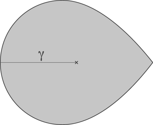
Figure 4: The base of the boundary Lefschetz fibration on $S^4$
together with a path expressing the Lefschetz and elliptic singularities as a dual pair.
$S^4$
together with a path expressing the Lefschetz and elliptic singularities as a dual pair.
The proof of this lemma is somewhat long, so we will postpone it to this end of this section.
Lemma 5.6 Let $(\mathbb {D}^4,D)$
be the open disk in
$(\mathbb {D}^4,D)$
be the open disk in $\mathbb {C}^2$
with divisor
$\mathbb {C}^2$
with divisor $I_{z_1}$
, and let
$I_{z_1}$
, and let $\mathbb {D}^2_+ \subset \mathbb {R}^2$
be the open half-disk with boundary in the real axis
$\mathbb {D}^2_+ \subset \mathbb {R}^2$
be the open half-disk with boundary in the real axis
 $$ \begin{align*} \mathbb{D}^2_+ = \{ (x,y) \in \mathbb{R}^2\colon x^2 + y^2 < 1 \mbox{ and } x\geq 0\}. \end{align*} $$
Then there is a proper boundary Lefschetz fibration with connected fibers, $f_{\mathbb {D}^4} \colon (\mathbb {D}^4,D) \to (\mathbb {D}^2_+,\partial \mathbb {D}^2_+)$
, such that:
$f_{\mathbb {D}^4} \colon (\mathbb {D}^4,D) \to (\mathbb {D}^2_+,\partial \mathbb {D}^2_+)$
, such that:
-
•
$f_{\mathbb {D}^4}$
has a single Lefschetz fiber. -
• The vanishing cycles of the Lefschetz fiber and the elliptic fiber form a dual pair.

Furthermore, if $f \colon (M,D) \to (\mathbb {D}^2_+,\partial \mathbb {D}^2_+)$
is a proper boundary Lefschetz fibration with connected fibers with the two properties above, then f is equivalent to
$f \colon (M,D) \to (\mathbb {D}^2_+,\partial \mathbb {D}^2_+)$
is a proper boundary Lefschetz fibration with connected fibers with the two properties above, then f is equivalent to $f_{\mathbb {D}^4}$
, that is, there is a commutative diagram:
$f_{\mathbb {D}^4}$
, that is, there is a commutative diagram:

where the horizontal maps are diffeomorphisms.
Proof The existence of the fibration $f_{\mathbb {D}^4}$
follows from Lemma 5.5. Indeed, we split the base of
$f_{\mathbb {D}^4}$
follows from Lemma 5.5. Indeed, we split the base of $f_{S^4}$
in two parts,
$f_{S^4}$
in two parts, $V_1$
, a neighborhood of the vertex, and
$V_1$
, a neighborhood of the vertex, and $V_2$
, the rest of the base plus a small overlap with
$V_2$
, the rest of the base plus a small overlap with $V_1$
, as indicated in Figure 5. Then, due to Lemma 3.8, on
$V_1$
, as indicated in Figure 5. Then, due to Lemma 3.8, on $f^{-1}(V_1)$
, in appropriate coordinates, we have
$f^{-1}(V_1)$
, in appropriate coordinates, we have
 $$ \begin{align*} V_1 = \{(x,y)\in \mathbb{R}^2\colon x+y <1, x \geq0, y\geq 0\}, \end{align*} $$
and the fibration is given by
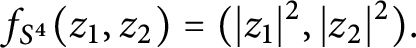 $$ \begin{align*} f_{S^4}(z_1,z_2) = (|z_1|^2,|z_2|^2). \end{align*} $$
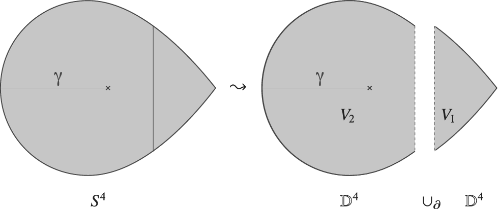
Figure 5: The base of the boundary Lefschetz fibration on $S^4$
split in two halves, each half being a fibration of
$S^4$
split in two halves, each half being a fibration of $\mathbb {D}^4$
.
$\mathbb {D}^4$
.
Hence, $f_{S^4}^{-1}(V_1)$
is a disk and its complement
$f_{S^4}^{-1}(V_1)$
is a disk and its complement $f_{S_4}^{-1}(V_2)$
is also a disk. However,
$f_{S_4}^{-1}(V_2)$
is also a disk. However,
 $$ \begin{align*} f_{S_4}|_{V_2}\colon V_2 \to f_{S^4}(V_2) \end{align*} $$
has all the properties required in the lemma after we choose a diffeomorphism between $V_2$
and
$V_2$
and $\mathbb {D}^2_+$
. Therefore, we have existence.
$\mathbb {D}^2_+$
. Therefore, we have existence.
To prove the uniqueness part, we study all possible ways such a fibration may arise. Let $f\colon M \rightarrow (\mathbb {D}^2_+,\partial \mathbb {D}^2_+)$
be a boundary Lefschetz fibration satisfying the assumptions of the lemma. Without loss of generality, we assume that the image of the Lefschetz singularity is
$f\colon M \rightarrow (\mathbb {D}^2_+,\partial \mathbb {D}^2_+)$
be a boundary Lefschetz fibration satisfying the assumptions of the lemma. Without loss of generality, we assume that the image of the Lefschetz singularity is $(2/3,0)$
, and we split
$(2/3,0)$
, and we split $\mathbb {D}^2_+$
in two parts:
$\mathbb {D}^2_+$
in two parts:
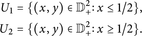 $$ \begin{align*} U_1 &= \{(x,y)\in \mathbb{D}^2_+\colon x \leq 1/2\},\\ U_2 &= \{(x,y)\in \mathbb{D}^2_+\colon x \geq 1/2\}. \end{align*} $$
The set $f^{-1}(U_2)$
is a neighborhood of the Lefschetz fiber, and hence its differentiable type as a fibration is fully determined [Reference Gompf and Stipsicz17]. Similarly, the set
$f^{-1}(U_2)$
is a neighborhood of the Lefschetz fiber, and hence its differentiable type as a fibration is fully determined [Reference Gompf and Stipsicz17]. Similarly, the set $f^{-1}(U_1)$
is a neighborhood of an elliptic fiber, and hence its differentiable type as a fibration is also fully determined:
$f^{-1}(U_1)$
is a neighborhood of an elliptic fiber, and hence its differentiable type as a fibration is also fully determined:
 $$ \begin{align*} f^{-1}(U_1) = \mathbb{D}^2 \times S^1 \times (-1,1), \quad f(re^{i\theta}, \psi, t) = (r^2,t). \end{align*} $$
Therefore, all possible different fibrations with the desired properties are determined by the different ways these two pieces can be glued together modulo the action of the isomorphism group of each half of the fibration.
Since the gluing takes place over a regular fibration over an interval, the isotopy class of the gluing map is determined by the isotopy class of the map it induces at a single fiber. Since the fibers are tori, this is in turn determined by the corresponding map in homology. Since the vanishing cycles form a dual pair, there is, modulo the action of the isomorphism group of the fibration over $V_1$
, a unique way to glue these together.▪
$V_1$
, a unique way to glue these together.▪
Next, we show how to use Lemmas 5.5 and 5.6 to prove both singularity trade theorems.
Proof Applying Theorem 4.6 to the boundary Lefschetz fibration on M and on $S^4$
gives rise to a boundary Lefschetz fibration on
$S^4$
gives rise to a boundary Lefschetz fibration on $M\# S^4\simeq M$
, for which the inclusion
$M\# S^4\simeq M$
, for which the inclusion $M\backslash \lbrace p \rbrace \hookrightarrow M$
preserves fibrations, in particular, we see that the new fibration on M only changes in the small ball around p used for the connected sum procedure. Since the divisor in
$M\backslash \lbrace p \rbrace \hookrightarrow M$
preserves fibrations, in particular, we see that the new fibration on M only changes in the small ball around p used for the connected sum procedure. Since the divisor in $S^4$
has only one point in the top stratum, the new divisor satisfies
$S^4$
has only one point in the top stratum, the new divisor satisfies $\widetilde D[2] = D[2] \backslash \{p\}$
, and
$\widetilde D[2] = D[2] \backslash \{p\}$
, and $\widetilde {D}$
and D have the same index. Given the way the fibrations are glued, we see that the effect on the base is to smooth out the corner corresponding to
$\widetilde {D}$
and D have the same index. Given the way the fibrations are glued, we see that the effect on the base is to smooth out the corner corresponding to $f(p)$
. Continuing inductively gives rise to a boundary Lefschetz fibration with embedded divisor. ▪
$f(p)$
. Continuing inductively gives rise to a boundary Lefschetz fibration with embedded divisor. ▪
Proof Under the conditions of the theorem, $\gamma $
has a neighborhood,
$\gamma $
has a neighborhood, $V_2$
, diffeomorphic to
$V_2$
, diffeomorphic to $\mathbb {D}_+^2$
in which the fibration has only one Lefschetz singularity whose vanishing cycle forms a dual pair with the elliptic singularity. Hence, by Lemma 5.6,
$\mathbb {D}_+^2$
in which the fibration has only one Lefschetz singularity whose vanishing cycle forms a dual pair with the elliptic singularity. Hence, by Lemma 5.6, $f^{-1}(V_2)$
is diffeomorphic to
$f^{-1}(V_2)$
is diffeomorphic to $\mathbb {D}^4$
, and f is equivalent to the fibration of Lemma 5.6. Since the fibration on
$\mathbb {D}^4$
, and f is equivalent to the fibration of Lemma 5.6. Since the fibration on $S^4$
splits as two disks, one fibering over
$S^4$
splits as two disks, one fibering over $\mathbb {D}_+^2$
and the other fibering over a neighborhood,
$\mathbb {D}_+^2$
and the other fibering over a neighborhood, $V_1$
, of the origin in
$V_1$
, of the origin in $(\mathbb {R}_+)^2$
(see Figure 5), we can realize
$(\mathbb {R}_+)^2$
(see Figure 5), we can realize $M \# S^4$
as follows: remove the disk
$M \# S^4$
as follows: remove the disk $f^{-1}(V_2)$
and glue back, by the natural identification of the boundary,
$f^{-1}(V_2)$
and glue back, by the natural identification of the boundary, $f_{S^4}^{-1}(V_1)$
.
$f_{S^4}^{-1}(V_1)$
.
Since this procedure corresponds to performing connected sum with $S^4$
, the final manifold is still diffeomorphic to M and the fibration only changes in the part that has been surged in, which includes the removal of the Lefschetz singularity from
$S^4$
, the final manifold is still diffeomorphic to M and the fibration only changes in the part that has been surged in, which includes the removal of the Lefschetz singularity from $f^{-1}(V_2)$
and the inclusion of the elliptic–elliptic singularity of
$f^{-1}(V_2)$
and the inclusion of the elliptic–elliptic singularity of $f_{S^4}^{-1}(V_1)$
. Finally, notice that the process of filling the boundary of
$f_{S^4}^{-1}(V_1)$
. Finally, notice that the process of filling the boundary of $f^{-1}(V_2)$
with
$f^{-1}(V_2)$
with $f_{S^4}^{-1}(V_1)$
is not compatible with the given orientations of these spaces, since they both appear at opposite sides of a boundary in
$f_{S^4}^{-1}(V_1)$
is not compatible with the given orientations of these spaces, since they both appear at opposite sides of a boundary in $S^4$
. That is, the orientation of M is compatible with the opposite orientation of
$S^4$
. That is, the orientation of M is compatible with the opposite orientation of $f_{S^4}^{-1}(V_1)$
. Since the elliptic–elliptic singularity for the fibration in
$f_{S^4}^{-1}(V_1)$
. Since the elliptic–elliptic singularity for the fibration in $S^4$
had index
$S^4$
had index $-1$
and the orientation of
$-1$
and the orientation of $S^4$
was reversed in the connected sum process, the intersection index of the new elliptic–elliptic singularity on M is
$S^4$
was reversed in the connected sum process, the intersection index of the new elliptic–elliptic singularity on M is $+1$
, and hence the overall parity of the divisor is unchanged.▪
$+1$
, and hence the overall parity of the divisor is unchanged.▪
To finish the proof of the trade theorems, we must establish Lemma 5.5, which we do next.
Proof The proof is done in two steps. In the first step, we show that if M is the total space of a boundary Lefschetz fibration whose singularities are as stated in Lemma 5.5, then $M = S^4$
. In the second step, we show that such a fibration exists.
$M = S^4$
. In the second step, we show that such a fibration exists.
Step 1. We observe once again that M is made of two fibrations glued together, as illustrated in Figure 5: one fibration with an elliptic–elliptic singularity over $V_1$
and one with a Lefschetz singularity over
$V_1$
and one with a Lefschetz singularity over $V_2$
. The fibration over
$V_2$
. The fibration over $V_1$
is a copy of
$V_1$
is a copy of $\mathbb {D}^4$
added along its
$\mathbb {D}^4$
added along its $S^3$
boundary, that is,
$S^3$
boundary, that is, $M = f^{-1}(V_2) \cup \mbox { 4-handle}$
. The space
$M = f^{-1}(V_2) \cup \mbox { 4-handle}$
. The space $f^{-1}(V_2)$
itself can be readily described as a handlebody: we start with a neighborhood of a regular fiber, then add a
$f^{-1}(V_2)$
itself can be readily described as a handlebody: we start with a neighborhood of a regular fiber, then add a $-1$
-framed
$-1$
-framed $2$
-handle along the vanishing cycle of the Lefschetz singularity to obtain a neighborhood of the Lefschetz singular fiber and a
$2$
-handle along the vanishing cycle of the Lefschetz singularity to obtain a neighborhood of the Lefschetz singular fiber and a $0$
-framed
$0$
-framed $2$
-handle along the vanishing cycle of the elliptic singularity. Therefore, the Kirby diagram of M is the one depicted in Figure 6a. We can then slide the
$2$
-handle along the vanishing cycle of the elliptic singularity. Therefore, the Kirby diagram of M is the one depicted in Figure 6a. We can then slide the $2$
-handle that goes around both 1-handles to obtain Figure 6b and see that the resulting
$2$
-handle that goes around both 1-handles to obtain Figure 6b and see that the resulting $2$
-handle separates as a
$2$
-handle separates as a $0$
-framed
$0$
-framed $2$
-handle from the rest of the diagram and hence cancels with the
$2$
-handle from the rest of the diagram and hence cancels with the $3$
-handle. The remaining pairs of
$3$
-handle. The remaining pairs of $1$
- and
$1$
- and $2$
-handles clearly cancel each other (Figure 6c), leaving us with the empty diagram, which corresponds to
$2$
-handles clearly cancel each other (Figure 6c), leaving us with the empty diagram, which corresponds to $S^4$
.
$S^4$
.
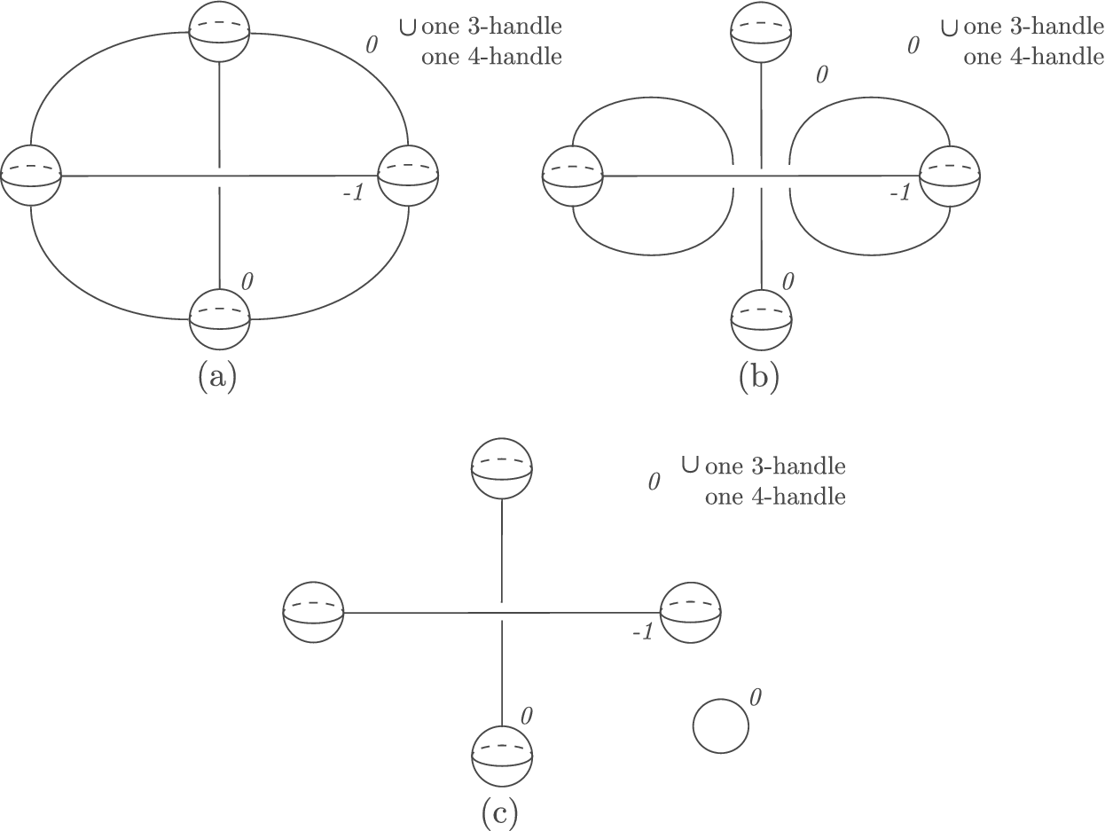
Figure 6: Kirby diagram for the total space of the fibration described in Lemma 5.6.
Step 2. To construct the desired fibration, we will use a plumbing construction applied to the disk bundle of $\mathcal {O}(2) \rightarrow \mathbb {C} P^1$
in a way that is compatible with the natural torus fibration of that space. Throughout, we will use fixed parameterizations
$\mathcal {O}(2) \rightarrow \mathbb {C} P^1$
in a way that is compatible with the natural torus fibration of that space. Throughout, we will use fixed parameterizations $\varphi _1,\varphi _2\colon \mathbb {C}^2 \to \mathcal {O}(2)$
for which the change of coordinates is given by
$\varphi _1,\varphi _2\colon \mathbb {C}^2 \to \mathcal {O}(2)$
for which the change of coordinates is given by
 $$ \begin{align*} \varphi_2^{-1} \circ \varphi_1(z,w) = (z^{-1},z^{-2}w). \end{align*} $$
We will refer to $\varphi _1$
as parameterizing a trivialization of
$\varphi _1$
as parameterizing a trivialization of $\mathcal {O}(2)$
with the south pole removed and similarly
$\mathcal {O}(2)$
with the south pole removed and similarly $\varphi _2$
does not cover the fiber over the north pole.
$\varphi _2$
does not cover the fiber over the north pole.
Rotation on both coordinates in the parameterization $\varphi _2$
give rise to a torus action on
$\varphi _2$
give rise to a torus action on $\mathcal {O}(2)$
which, in the parameterizations above, is given by
$\mathcal {O}(2)$
which, in the parameterizations above, is given by
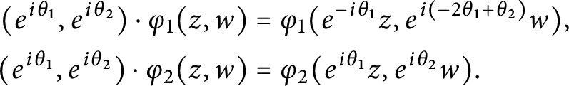 $$ \begin{align} \begin{aligned} (e^{i \theta_1},e^{i\theta_2})\cdot \varphi_1(z,w) &= \varphi_1(e^{-i\theta_1}z,e^{i(-2\theta_1+\theta_2)}w),\\ (e^{i \theta_1},e^{i \theta_2})\cdot \varphi_2(z,w) &= \varphi_2(e^{i\theta_1}z,e^{i\theta_2}w). \end{aligned} \end{align} $$
To describe the quotient of $\mathcal {O}(2)$
by this torus action, we will also want to consider
$\mathcal {O}(2)$
by this torus action, we will also want to consider $[-1,1]\times \mathbb {R}_+$
. Of course, this space can be parameterized by a single, rather obvious, chart, but it will be convenient to parameterize it by two charts instead. We consider the parameterizations
$[-1,1]\times \mathbb {R}_+$
. Of course, this space can be parameterized by a single, rather obvious, chart, but it will be convenient to parameterize it by two charts instead. We consider the parameterizations
 $$ \begin{align*} \psi_1 \colon \mathbb{R}_+\times \mathbb{R}_+ \to (-1,1] \times \mathbb{R}_+ \subset [-1,1] \times \mathbb{R}_+ \qquad \psi_1(x_1,y_1) = \left(\frac{1-x_1}{1+ x_1},\frac{y_1}{(1+x_1)^2}\right), \end{align*} $$
 $$ \begin{align*} \psi_2 \colon \mathbb{R}_+\times \mathbb{R}_+ \to [-1,1) \times \mathbb{R}_+ \subset [-1,1] \times \mathbb{R}_+ \qquad \psi_2(x_2,y_2) = \left(-\frac{1-x_2}{1+ x_2},\frac{y_2}{(1+x_2)^2}\right), \end{align*} $$
and keep in mind that these parameterizations induce opposite orientations, with $\psi _2$
agreeing with the natural orientation of
$\psi _2$
agreeing with the natural orientation of $[-1,1]\times \mathbb {R}_+$
.
$[-1,1]\times \mathbb {R}_+$
.
Lemma 5.7 If we let $h\colon S^2 \rightarrow \mathbb {R}$
be the height function and
$h\colon S^2 \rightarrow \mathbb {R}$
be the height function and $g\colon \mathrm {Sym}^2\mathcal {O}(2) \rightarrow \mathbb {R}$
be the Fubini–Study metric, then
$g\colon \mathrm {Sym}^2\mathcal {O}(2) \rightarrow \mathbb {R}$
be the Fubini–Study metric, then
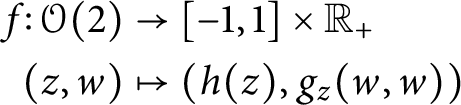 $$ \begin{align*} f\colon \mathcal{O}(2) &\rightarrow [-1,1]\times \mathbb{R}_+\\ (z,w) &\mapsto (h(z),g_z(w,w)) \end{align*} $$
defines a quotient map for the torus action on $\mathcal {O}(2)$
. Furthermore, f is a proper boundary fibration with elliptic divisor induced by the holomorphic log divisor consisting of the zero section and fibers over the north and south poles.▪
$\mathcal {O}(2)$
. Furthermore, f is a proper boundary fibration with elliptic divisor induced by the holomorphic log divisor consisting of the zero section and fibers over the north and south poles.▪
Proof In the parameterizations $\varphi _i$
, the height and distance functions take the form:
$\varphi _i$
, the height and distance functions take the form:
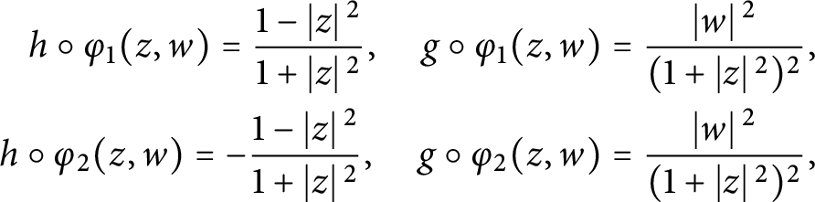 $$ \begin{align*} h\circ \varphi_1(z,w) = \frac{1-\left| z \right|{}^2}{1+\left| z \right|{}^2}, \quad g\circ \varphi_1(z,w) = \frac{\left| w \right|{}^2}{(1+\left| z \right|{}^2)^2},\\ h\circ \varphi_2(z,w) = -\frac{1-\left| z \right|{}^2}{1+\left| z \right|{}^2}, \quad g\circ \varphi_2(z,w) = \frac{\left| w \right|{}^2}{(1+\left| z \right|{}^2)^2}, \end{align*} $$
which are clearly invariant under the $T^2$
-action in equation (5.1). Furthermore, for
$T^2$
-action in equation (5.1). Furthermore, for $i=1,2$
, the image of
$i=1,2$
, the image of $f\circ \varphi _i$
lands in the image of the parameterization
$f\circ \varphi _i$
lands in the image of the parameterization $\psi _i$
, and we can compute the expression for f in these parameterizations:
$\psi _i$
, and we can compute the expression for f in these parameterizations:
 $$ \begin{align} f_i(z,w) := \psi_i^{-1} \circ f \circ \varphi_i(z,w) = (|z|^2,|w|^2), \end{align} $$
which shows clearly that f is not only the quotient map, but also a boundary fibration.▪
Now, we perform a plumbing on $\mathcal {O}(2)$
.
$\mathcal {O}(2)$
.
Definition 5.8 Let $\pi \colon M^{2n} \rightarrow N^n$
be a
$\pi \colon M^{2n} \rightarrow N^n$
be a $\mathbb {D}^n$
-bundle, and let
$\mathbb {D}^n$
-bundle, and let $\mathbb {D}_1,\mathbb {D}_2$
be disjoint disks in N over which
$\mathbb {D}_1,\mathbb {D}_2$
be disjoint disks in N over which $\pi $
is trivializable. A self-plumbing of
$\pi $
is trivializable. A self-plumbing of $\pi $
at
$\pi $
at $\mathbb {D}_1$
and
$\mathbb {D}_1$
and $\mathbb {D}_2$
is obtained by identifying
$\mathbb {D}_2$
is obtained by identifying $\pi ^{-1}(\mathbb {D}_1)\simeq \mathbb {D}_1\times \mathbb {D}^n$
and
$\pi ^{-1}(\mathbb {D}_1)\simeq \mathbb {D}_1\times \mathbb {D}^n$
and $\pi ^{-1}(\mathbb {D}_2)\simeq \mathbb {D}_2 \times \mathbb {D}^n$
using a map which preserves the product structure but reverses the factors.
$\pi ^{-1}(\mathbb {D}_2)\simeq \mathbb {D}_2 \times \mathbb {D}^n$
using a map which preserves the product structure but reverses the factors.
For the case at hand, let $\mathbb {D}^2\mathcal {O}(2)$
be the open
$\mathbb {D}^2\mathcal {O}(2)$
be the open $\varepsilon $
-disk bundle with respect to the Fubini–Study metric. By restricting f to
$\varepsilon $
-disk bundle with respect to the Fubini–Study metric. By restricting f to $\mathbb {D}^2\mathcal {O}(2)$
, we obtain a proper boundary fibration
$\mathbb {D}^2\mathcal {O}(2)$
, we obtain a proper boundary fibration $f\colon \mathbb {D}^2\mathcal {O}(2) \rightarrow [-1,1]\times [0,\varepsilon )$
.
$f\colon \mathbb {D}^2\mathcal {O}(2) \rightarrow [-1,1]\times [0,\varepsilon )$
.
Furthermore, we observe that $\varphi _1$
and
$\varphi _1$
and $\varphi _2$
provide trivializations of
$\varphi _2$
provide trivializations of $\mathbb {D}^2\mathcal {O}(2)$
, and hence we can use them to perform a self-plumbing of
$\mathbb {D}^2\mathcal {O}(2)$
, and hence we can use them to perform a self-plumbing of $\mathbb {D}^2\mathcal {O}(2)$
at the north and south poles. Let M be defined as the self-plumbing of
$\mathbb {D}^2\mathcal {O}(2)$
at the north and south poles. Let M be defined as the self-plumbing of $\mathbb {D}^2\mathcal {O}(2)$
via the trivializations
$\mathbb {D}^2\mathcal {O}(2)$
via the trivializations $\varphi _i$
and the map
$\varphi _i$
and the map
 $$ \begin{align*} \Phi\colon \mathbb{C}^2 \rightarrow \mathbb{C}^2 : (z,w)&\mapsto (\overline{w},\overline{z}), \end{align*} $$
that is, $\varphi _1(z,w)$
is identified with
$\varphi _1(z,w)$
is identified with $\varphi _2(\overline {w},\overline {z})$
.
$\varphi _2(\overline {w},\overline {z})$
.
Since the map used for the plumbing preserves elliptic ideals and identifies the north and south poles, M is endowed with an elliptic divisor with a single point in $D[2]$
. Since the map
$D[2]$
. Since the map $\Phi $
does not match co-orientations, the elliptic divisor in M has intersection index
$\Phi $
does not match co-orientations, the elliptic divisor in M has intersection index $-1$
.
$-1$
.
To endow M with a boundary fibration, we only need to take a quotient of the base, $[-1,1]\times [0,\varepsilon )$
, by the equivalence relation that makes the following diagram commute:
$[-1,1]\times [0,\varepsilon )$
, by the equivalence relation that makes the following diagram commute:
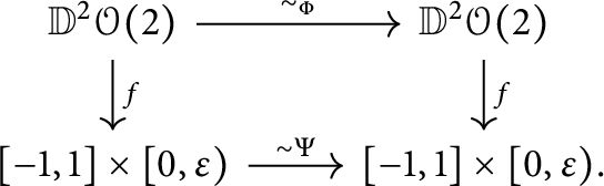
Since f is surjective, there is a unique identification, $\sim _{\Psi }$
, that gives rise to such a diagram. In fact, we can easily compute it in the parameterizations
$\sim _{\Psi }$
, that gives rise to such a diagram. In fact, we can easily compute it in the parameterizations $\psi _i$
, where it is induced by the map
$\psi _i$
, where it is induced by the map $\Psi (x,y) = (1-y,x+1)$
. That is, the point
$\Psi (x,y) = (1-y,x+1)$
. That is, the point $\psi _1(x,y)$
is identified with the point
$\psi _1(x,y)$
is identified with the point $\psi _2(y,x)$
. Since
$\psi _2(y,x)$
. Since $\psi _1$
and
$\psi _1$
and $\psi _2$
induce opposite orientations, this identification preserves the natural orientation of
$\psi _2$
induce opposite orientations, this identification preserves the natural orientation of $[-1,1]\times [0,\varepsilon )$
and the quotient is an oriented half-open cylinder with one corner (see Figure 7).
$[-1,1]\times [0,\varepsilon )$
and the quotient is an oriented half-open cylinder with one corner (see Figure 7).
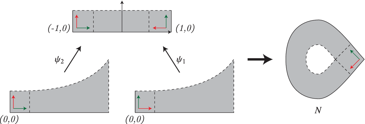
Figure 7: The base of the boundary fibration constructed in Lemma 5.9.
Lemma 5.9 The map $f\colon \mathbb {D}^2\mathcal {O}(2) \rightarrow [-1,1]\times [0,\varepsilon )$
descends to a boundary fibration
$f\colon \mathbb {D}^2\mathcal {O}(2) \rightarrow [-1,1]\times [0,\varepsilon )$
descends to a boundary fibration $\hat {f}\colon M \rightarrow N$
.
$\hat {f}\colon M \rightarrow N$
.
Next, we compute its monodromy along a generator of $\pi _1(N)$
.
$\pi _1(N)$
.
Lemma 5.10 Let $\hat {f}\colon M \rightarrow N$
be the boundary fibration from Lemma 5.9. Then the monodromy of
$\hat {f}\colon M \rightarrow N$
be the boundary fibration from Lemma 5.9. Then the monodromy of $\hat {f}$
around a loop around the hole is a positive Dehn twist.
$\hat {f}$
around a loop around the hole is a positive Dehn twist.
Proof This is a direct computation using the given change of coordinates and the plumbing map $\Phi $
. Indeed, all we need to do is to track what happens with the torus action as we move along from the chart covered by
$\Phi $
. Indeed, all we need to do is to track what happens with the torus action as we move along from the chart covered by $\varphi _2$
to the chart covered by
$\varphi _2$
to the chart covered by $\varphi _1$
and then back to
$\varphi _1$
and then back to $\varphi _2$
via
$\varphi _2$
via $\Psi $
:
$\Psi $
:
 $$ \begin{align*} (e^{i\theta_1}, e^{i\theta_2}) & \cdot\varphi_2(z,w) =\varphi_2(e^{i\theta_1}z,e^{i\theta_2}w) =\varphi_1(e^{-i\theta_1}z^{-1},e^{i(-2\theta_1 + \theta_2)}z^{-2}w) \\ & \sim_{\Phi} \varphi_2(e^{i(2\theta_1 - \theta_2)}\overline{z}^{{\kern1pt}-2}\overline{w},e^{i\theta_1}\overline{z}^{{\kern1pt}-1}) = (e^{i(2\theta_1 - \theta_2)},e^{i\theta_1})\varphi_2(\overline{z}^{{\kern1pt}-2}\overline{w}, \overline{z}^{{\kern1pt}-1}). \end{align*} $$
Therefore, we see that, in the basis $\{e_{\theta _1},e_{\theta _2}\}$
for
$\{e_{\theta _1},e_{\theta _2}\}$
for $H^1(F)$
corresponding to the generators of the action, the monodromy transformation is given by the matrix
$H^1(F)$
corresponding to the generators of the action, the monodromy transformation is given by the matrix
 $$ \begin{align*} \begin{pmatrix} 2 & -1\\ 1 &0 \end{pmatrix}. \end{align*} $$
Notice that using the complex orientation of $\mathcal {O}(2)$
and the standard orientation of
$\mathcal {O}(2)$
and the standard orientation of $\mathbb {R}^2$
,
$\mathbb {R}^2$
, $\{e_{\theta _1},e_{\theta _2}\}$
is a negative basis for the homology of the fiber. Using this, we see that the transformation above is a positive Dehn twist on the cycle
$\{e_{\theta _1},e_{\theta _2}\}$
is a negative basis for the homology of the fiber. Using this, we see that the transformation above is a positive Dehn twist on the cycle $e_{\theta _1}+ e_{\theta _2}$
.▪
$e_{\theta _1}+ e_{\theta _2}$
.▪
Now, we can complete M to a closed manifold by glueing a neighborhood of a single Lefschetz fiber with vanishing cycle $e_{\theta _1} + e_{\theta _2}$
in the hole of the annulus. Finally, we observe that this vanishing cycle forms a dual pair with either of the two vanishing cycles of the elliptic singularity, which in the parameterization
$e_{\theta _1} + e_{\theta _2}$
in the hole of the annulus. Finally, we observe that this vanishing cycle forms a dual pair with either of the two vanishing cycles of the elliptic singularity, which in the parameterization $\varphi _2$
are given by either of the cycles
$\varphi _2$
are given by either of the cycles $e_{\theta _1}$
or
$e_{\theta _1}$
or $e_{\theta _2}$
.
$e_{\theta _2}$
.
Remark 5.11 Simply drawing a base diagram for a boundary Lefschetz fibration does not guarantee the existence of a fibration that realizes it. For example, there is no manifold whose base diagram is that of Figure 4, but for which the elliptic–elliptic singularity has intersection index $1$
. In the construction above, this would manifest itself in the fact that, without using complex conjugation, the monodromy of the plumbing would be a negative Dehn twist. This highlights that the long second step in the proof above is indeed necessary.
$1$
. In the construction above, this would manifest itself in the fact that, without using complex conjugation, the monodromy of the plumbing would be a negative Dehn twist. This highlights that the long second step in the proof above is indeed necessary.
6 Examples
In this section, we give several concrete examples of boundary fibrations. We will first show that they arise naturally as the quotient maps of effective torus actions, and that our framework fits particularly well with the theory of integrable systems. This connection provides us immediately with a wealth of examples of both boundary fibrations and stable generalized complex structures. We will further illustrate our constructions by showing how starting with simple examples (of manifolds with torus actions) we can use the connected sum procedure to obtain many more examples of boundary fibrations.
6.1 Torus actions
We show that quotient maps of torus actions provide boundary fibrations.
Proposition 6.1 Let $T^n$
act effectively on a smooth manifold
$T^n$
act effectively on a smooth manifold $M^{2n}$
, with connected isotropy groups. Then:
$M^{2n}$
, with connected isotropy groups. Then:
-
•
$N:= M^{2n}/T^n$
is a manifold with corners. -
• The quotient map defines a boundary fibration
$f\colon (M,D) \rightarrow (N,\partial N)$
with connected fibers. -
• The intersection stratification of the elliptic ideal coincides with the stratification by orbit types on M.
-
•
$ND[1]$
is co-orientable. -
• If M is oriented, then so is N.
-
• If M is four-dimensional and the action is not free, f is homologically essential.


Proof Let $p \in M$
, let
$p \in M$
, let $G_p$
denote the isotropy group of p, and let
$G_p$
denote the isotropy group of p, and let $\mathcal {O}_p$
denote the orbit of p. By assumption,
$\mathcal {O}_p$
denote the orbit of p. By assumption, $G_p$
is connected and therefore isomorphic to
$G_p$
is connected and therefore isomorphic to $T^{\ell }$
for some
$T^{\ell }$
for some $\ell \leq n$
. By the slice theorem, there exists a neighborhood of
$\ell \leq n$
. By the slice theorem, there exists a neighborhood of $\mathcal {O}_p$
which is equivariantly diffeomorphic to a neighborhood of the zero section in
$\mathcal {O}_p$
which is equivariantly diffeomorphic to a neighborhood of the zero section in
 $$ \begin{align*} G \times_{G_p} N_p\mathcal{O}_p, \end{align*} $$
where $G_p$
acts linearly on
$G_p$
acts linearly on $N_p\mathcal {O}_p$
by the differentiated action. Because all groups in consideration are abelian and connected, this implies that there is a neighborhood U around p of the form
$N_p\mathcal {O}_p$
by the differentiated action. Because all groups in consideration are abelian and connected, this implies that there is a neighborhood U around p of the form
 $$ \begin{align*} U = T^{n-\ell} \times (\mathbb{R}^{n-\ell}\times \mathbb{C}^{\ell}). \end{align*} $$
The $T^n = (T^{n-\ell }\times T^{\ell })$
-action of U decomposes as
$T^n = (T^{n-\ell }\times T^{\ell })$
-action of U decomposes as $T^{n-\ell }$
acting by multiplication on
$T^{n-\ell }$
acting by multiplication on $T^{n-\ell }$
and
$T^{n-\ell }$
and $T^{\ell }$
acting linearly on
$T^{\ell }$
acting linearly on $\mathbb {C}^{\ell }$
. Since the irreducible representations of
$\mathbb {C}^{\ell }$
. Since the irreducible representations of $T^{\ell }$
are one-dimensional, we may without loss of generality assume that each coordinate line in
$T^{\ell }$
are one-dimensional, we may without loss of generality assume that each coordinate line in $\mathbb {C}^{\ell }$
is preserved by the action. Therefore, if we let
$\mathbb {C}^{\ell }$
is preserved by the action. Therefore, if we let $\mathfrak {t}$
denote the Lie algebra of
$\mathfrak {t}$
denote the Lie algebra of $T^{\ell }$
, let
$T^{\ell }$
, let $\mathfrak {l}$
denote the kernel of
$\mathfrak {l}$
denote the kernel of $\exp \colon \mathfrak {t} \rightarrow T^{\ell }$
, with minimal generating set
$\exp \colon \mathfrak {t} \rightarrow T^{\ell }$
, with minimal generating set $\{\xi _1,\dots ,\xi _{\ell }\}$
and choose
$\{\xi _1,\dots ,\xi _{\ell }\}$
and choose $\{\alpha _1,\ldots ,\alpha _{\ell }\} \in \mathfrak {l}^*$
the dual basis for the dual lattice, then the action on each irreducible representation has the form
$\{\alpha _1,\ldots ,\alpha _{\ell }\} \in \mathfrak {l}^*$
the dual basis for the dual lattice, then the action on each irreducible representation has the form
 $$ \begin{align*} \exp(\Theta)\cdot z_j = e^{2\pi i \left\langle \Theta,n_j\alpha_j \right\rangle}z_j, \qquad \Theta \in \mathfrak{t}. \end{align*} $$
Since the action is effective, we have that $n_j \neq 0$
, and because the isotropy groups are connected, we must furthermore have
$n_j \neq 0$
, and because the isotropy groups are connected, we must furthermore have $n_j = \pm 1$
. Hence, after appropriately changing the signs of some of the
$n_j = \pm 1$
. Hence, after appropriately changing the signs of some of the $\alpha _j$
, the
$\alpha _j$
, the $T^{\ell }$
-action is given by
$T^{\ell }$
-action is given by
 $$ \begin{align*} (\exp(\theta_1\xi_1\cdot \ldots \cdot \theta_{\ell}\xi_{\ell}))\cdot (z_1,\ldots,z_{\ell}) = (e^{2\pi \theta_1 i}z_1,\ldots e^{2\pi \theta_{\ell} i}z_{\ell}). \end{align*} $$
This normal form for the action has the following consequences:
-
• The quotient manifold is endowed with charts of the form
$\mathbb {R}^{n-\ell } \times (\mathbb {C}^{\ell })/T^{\ell } \simeq \mathbb {R}^n_{\ell }$
, and is therefore a manifold with corners. -
• The quotient map
$f\colon M \rightarrow N$
in the above local coordinates is given by
$$ \begin{align*} f\colon T^{n-\ell} \times (\mathbb{R}^{n-\ell}\times \mathbb{C}^{\ell}) &\rightarrow \mathbb{R}^n_{\ell}\\ (q,x,z_1,\ldots,z_{\ell}) &\mapsto (x,\left| z_1 \right|{}^2,\ldots,\left| z_{\ell} \right|{}^2). \end{align*} $$
By Lemma 3.8, we see that f is a boundary fibration with respect to the log divisor
$\partial N$
. -
• Because the vanishing locus of the induced elliptic ideal is given by
$f^{-1}(\partial N)$
, it follows that the intersection stratification coincides with the orbit-type stratification. -
• At points
$p \in D[1]$
, the isotropy group is given by
$S^1$
, and therefore
$N_p\mathcal {O}_p$
inherits an
$S^1$
-action and consequently admits an orientation. We conclude that
$D[1]$
is co-orientable. -
• When M is oriented, a choice of orientation for
$T^n$
gives rise to an orientation for N by observing that
$M\backslash D \rightarrow N \backslash \partial N$
is a principal
$T^n$
-bundle. -
• When M is four-dimensional and the action is not free, it is shown in [Reference Orlik and Raymond27] that f admits a section. As a generic fiber and the image of this section intersect only once, it follows that the intersection pairing of the fiber with the image of this section is nonzero, and therefore f is homologically essential.▪


The group actions underlying toric manifolds satisfy the conditions of this proposition, leading to the following result.
Corollary 6.2 Let $(M^{2n},\omega )$
be a toric manifold, and let
$(M^{2n},\omega )$
be a toric manifold, and let $f\colon M^{2n} \rightarrow \Delta ^n$
denote the quotient map. Then f is a boundary fibration.
$f\colon M^{2n} \rightarrow \Delta ^n$
denote the quotient map. Then f is a boundary fibration.
In four dimensions, Proposition 6.1 provides us with fibrations that satisfy nearly all the assumptions required to apply Theorem 3.23. However, the torus action does not guarantee that the parity of the elliptic divisor is 1. To proceed, we must add hypotheses to ensure that this is the case.
Proposition 6.3 Let $f\colon (M^4,\omega ) \rightarrow \mathbb {R}^2$
be a toric manifold. Then the parity of the elliptic divisor obtained from Proposition 6.1 is
$f\colon (M^4,\omega ) \rightarrow \mathbb {R}^2$
be a toric manifold. Then the parity of the elliptic divisor obtained from Proposition 6.1 is $1$
, and therefore M admits a stable generalized complex structure compatible with f.
$1$
, and therefore M admits a stable generalized complex structure compatible with f.
Proof By Proposition 6.1, we have that f is a boundary fibration, and therefore by Theorem 3.23 the manifold M admits an elliptic symplectic structure. As each of the preimages of the faces of the moment polytope is a symplectic submanifold of $(M,\omega )$
, the symplectic structure provides each component of the elliptic divisor with a natural co-orientation for which the intersections have positive index. It follows that the parity of the elliptic divisor is
$(M,\omega )$
, the symplectic structure provides each component of the elliptic divisor with a natural co-orientation for which the intersections have positive index. It follows that the parity of the elliptic divisor is $1$
.▪
$1$
.▪
6.2 Simple examples
We give examples of boundary fibrations obtained from torus actions which will serve as the building blocks for the connected sum procedure.
Example 6.4 (
$\mathbb {C}P^2$
)

Consider the standard toric structure on $\mathbb {C} P^2$
. Proposition 6.3 implies that f is a homologically essential boundary fibration and that
$\mathbb {C} P^2$
. Proposition 6.3 implies that f is a homologically essential boundary fibration and that $\mathbb {C}P^2$
admits an elliptic divisor with parity
$\mathbb {C}P^2$
admits an elliptic divisor with parity $1$
(three lines intersecting at different points). Therefore,
$1$
(three lines intersecting at different points). Therefore, $\mathbb {C} P^2$
admits a stable generalized complex structure compatible with its moment map.
$\mathbb {C} P^2$
admits a stable generalized complex structure compatible with its moment map.
Example 6.5 (
$\overline {\mathbb {C}P}^2$
)

We consider $\overline {\mathbb {C} P}^2$
, i.e.,
$\overline {\mathbb {C} P}^2$
, i.e., $\mathbb {C} P^2$
with the orientation opposite to the standard complex structure. As an oriented manifold, this is not a toric manifold, but there is still a
$\mathbb {C} P^2$
with the orientation opposite to the standard complex structure. As an oriented manifold, this is not a toric manifold, but there is still a $T^2$
-action with connected isotropies present. Therefore, Proposition 6.1 implies that the quotient map is a homologically essential boundary fibration. Consequently, by Theorem 3.23, there exists a compatible elliptic symplectic structure with imaginary parameter on
$T^2$
-action with connected isotropies present. Therefore, Proposition 6.1 implies that the quotient map is a homologically essential boundary fibration. Consequently, by Theorem 3.23, there exists a compatible elliptic symplectic structure with imaginary parameter on $\overline {\mathbb {C} P}^2$
. The parity of the elliptic divisor is
$\overline {\mathbb {C} P}^2$
. The parity of the elliptic divisor is $-1$
, so this symplectic structure does not induce a stable generalized complex structure. As
$-1$
, so this symplectic structure does not induce a stable generalized complex structure. As $\overline {\mathbb {C} P}^2$
is not almost complex, it cannot have a stable generalized complex structure, and hence this problem cannot be remedied.
$\overline {\mathbb {C} P}^2$
is not almost complex, it cannot have a stable generalized complex structure, and hence this problem cannot be remedied.
Example 6.6 (
$S^2\times S^2$
)

Let $(S^2\times S^2)$
be given its standard toric structure, i.e., the symplectic form is the product of the standard area forms and
$(S^2\times S^2)$
be given its standard toric structure, i.e., the symplectic form is the product of the standard area forms and $T^2$
acts on rotation by
$T^2$
acts on rotation by $S^1$
one each of the factors. Proposition 6.3 implies that the quotient map is a homologically essential boundary fibration and that
$S^1$
one each of the factors. Proposition 6.3 implies that the quotient map is a homologically essential boundary fibration and that $S^2\times S^2$
admits a compatible stable generalized complex structure.
$S^2\times S^2$
admits a compatible stable generalized complex structure.
Example 6.7 (
$S^4$
)

Consider $S^4 \subset \mathbb {C}^2 \times \mathbb {R}$
, and let
$S^4 \subset \mathbb {C}^2 \times \mathbb {R}$
, and let $T^2$
act in the standard way on
$T^2$
act in the standard way on $\mathbb {C}^2$
. This provides an effective
$\mathbb {C}^2$
. This provides an effective $T^2$
-action on
$T^2$
-action on $S^4$
with connected isotropies. Therefore, by Proposition 6.1, we find that the quotient map is a homologically essential boundary fibration. Consequently, Theorem 3.23 implies the existence of a compatible elliptic symplectic structure with imaginary parameter on
$S^4$
with connected isotropies. Therefore, by Proposition 6.1, we find that the quotient map is a homologically essential boundary fibration. Consequently, Theorem 3.23 implies the existence of a compatible elliptic symplectic structure with imaginary parameter on $S^4$
. The parity of the divisor is
$S^4$
. The parity of the divisor is $-1$
. Just as
$-1$
. Just as $\overline {\mathbb {C} P^2}$
,
$\overline {\mathbb {C} P^2}$
, $S^4$
is not almost-complex, so the index cannot be fixed by making different choices of divisor or orientations.
$S^4$
is not almost-complex, so the index cannot be fixed by making different choices of divisor or orientations.
The following example of a boundary fibration appears also in [Reference Cavalcanti and Klaasse9].
Example 6.8 (
$S^3\times S^1$
)

There are two interesting $T^2$
-actions on
$T^2$
-actions on $S^3\times S^1$
. First, consider
$S^3\times S^1$
. First, consider $S^3 \subset \mathbb {C}^2$
as the unit sphere and restrict the natural
$S^3 \subset \mathbb {C}^2$
as the unit sphere and restrict the natural $T^2$
-action on
$T^2$
-action on $\mathbb {C}^2$
to
$\mathbb {C}^2$
to $S^3$
. This provides an effective
$S^3$
. This provides an effective $T^2$
-action on
$T^2$
-action on $S^3$
with
$S^3$
with $S^1$
isotropy at all points in the intersection with the coordinate hyperplanes. Extending the
$S^1$
isotropy at all points in the intersection with the coordinate hyperplanes. Extending the $T^2$
-action trivially to the
$T^2$
-action trivially to the $S^1$
-factor provides an effective
$S^1$
-factor provides an effective $T^2$
-action on
$T^2$
-action on $S^3 \times S^1$
with only
$S^3 \times S^1$
with only $S^1$
isotropy groups. The quotient map
$S^1$
isotropy groups. The quotient map
 $$ \begin{align*} f_1\colon (S^3\times S^1,D_1) \rightarrow (I\times S^1,\lbrace 0,1 \rbrace\times S^1) \end{align*} $$
then becomes a homologically essential boundary fibration by Proposition 6.1. Note that $D_1$
is given by the union of two disjoint tori.
$D_1$
is given by the union of two disjoint tori.
Another $T^2$
-action on
$T^2$
-action on $S^3\times S^1$
is obtained by letting one
$S^3\times S^1$
is obtained by letting one $S^1$
act by rotation on one of the coordinates of
$S^1$
act by rotation on one of the coordinates of $S^3 \subset \mathbb {C}^2$
, and let the other act by multiplication on
$S^3 \subset \mathbb {C}^2$
, and let the other act by multiplication on $S^1$
. The quotient map
$S^1$
. The quotient map
 $$ \begin{align*} f_2\colon (S^3\times S^1,D_2) \rightarrow (\mathbb{D}^2,\partial \mathbb{D}^2) \end{align*} $$
then again becomes a homologically essential boundary fibration by Proposition 6.1. In this case, $D_2$
is a single torus. In both cases, Theorem 3.23 implies the existence of a compatible elliptic symplectic structure with zero elliptic residue. Moreover, as the vanishing locus of the elliptic divisor is smooth and co-orientable, we obtain two stable generalized complex structures on
$D_2$
is a single torus. In both cases, Theorem 3.23 implies the existence of a compatible elliptic symplectic structure with zero elliptic residue. Moreover, as the vanishing locus of the elliptic divisor is smooth and co-orientable, we obtain two stable generalized complex structures on $S^3\times S^1$
.
$S^3\times S^1$
.
The example we consider next is more elaborate than the previous ones. The existence of stable generalized complex structures on these spaces is a consequence of the more general Theorem 2 from [Reference Torres and Yazinski31].
Example 6.9 (
$(\#nS^1\times S^2)\times S^1$
)

In [Reference Orlik and Raymond27], it is shown that for $2g+h>1$
, the manifold
$2g+h>1$
, the manifold $M= (\#( 2g+h -1) S^1\times S^2)\times S^1$
admits an effective
$M= (\#( 2g+h -1) S^1\times S^2)\times S^1$
admits an effective $T^2$
-action with connected isotropy groups over a base, B, which is a surface of genus g with h small open disks removed. In fact, part of the action is just rotation of the last
$T^2$
-action with connected isotropy groups over a base, B, which is a surface of genus g with h small open disks removed. In fact, part of the action is just rotation of the last $S^1$
-factor, so this action has no fixed points (a fact that also follows from the Euler characteristic of M being
$S^1$
-factor, so this action has no fixed points (a fact that also follows from the Euler characteristic of M being $0$
).
$0$
).
By Proposition 6.1, we conclude that there exists a homologically essential boundary fibration
 $$ \begin{align*} f\colon ((\#(2g+h-1)S^1\times S^2)\times S^1,D) \rightarrow (B,\partial B). \end{align*} $$
The degeneracy locus consists of h disjoint tori—precisely, the number of boundary components of B, and is in particular co-orientable. Consequently, by Theorem 3.23, there exists a compatible (smooth) stable generalized complex structure on M whose type change locus has h connected components.
To illustrate the elliptic-elliptic trade theorem we give some examples:
Example 6.10 (
$\mathbb {C}P^2$
)

Applying Theorem 5.3 to Example 6.4 yields several boundary Lefschetz fibrations $f\colon (\mathbb {C}P^2,D) \rightarrow (N, \partial N)$
. The number of elliptic–elliptic and Lefschetz singularities adds up to 3, but any combination is possible. See also Figure 1 and Remark 6.13.
$f\colon (\mathbb {C}P^2,D) \rightarrow (N, \partial N)$
. The number of elliptic–elliptic and Lefschetz singularities adds up to 3, but any combination is possible. See also Figure 1 and Remark 6.13.
Example 6.11 (
$S^4$
)

Applying Theorem 5.3 to Example 6.7 yields a boundary Lefschetz fibration $f\colon (S^4,\widetilde {D}) \rightarrow (\mathbb {D}^2,\partial \mathbb {D}^2)$
with two Lefschetz singularities. Because the parity of the original divisor on
$f\colon (S^4,\widetilde {D}) \rightarrow (\mathbb {D}^2,\partial \mathbb {D}^2)$
with two Lefschetz singularities. Because the parity of the original divisor on $S^4$
is
$S^4$
is $-1$
, the new divisor
$-1$
, the new divisor $\widetilde {D}$
will be non-co-orientable. Therefore, it is nonorientable, and as it admits an
$\widetilde {D}$
will be non-co-orientable. Therefore, it is nonorientable, and as it admits an $S^1$
-fibration, it must then be a Klein bottle.
$S^1$
-fibration, it must then be a Klein bottle.
6.3 Main class of examples
Using the above examples as building blocks, we can now construct many more examples.
Theorem 6.12 The manifolds in the following two families admit homologically essential boundary fibrations:
-
•
$X_{n,\ell } := \#n(S^2\times S^2)\#\ell (S^1\times S^3)$
, with
$n,\ell \in \mathbb {N}$
, -
•
$Y_{n,m,\ell } := \#n \mathbb {C} P^2 \#m \overline {\mathbb {C}P}^2\#\ell (S^1 \times S^3)$
, with
$n,m,\ell \in \mathbb {N}$
,


whenever their Euler characteristic is nonnegative. Therefore, each of these manifolds admits a compatible elliptic symplectic structure, which induces a stable generalized complex structure if $1-b_1 + b_2^+$
is even.
$1-b_1 + b_2^+$
is even.
Proof In the previous section, we exhibited boundary fibrations on $\mathbb {C} P^2,\overline {\mathbb {C}P}^2$
and
$\mathbb {C} P^2,\overline {\mathbb {C}P}^2$
and $S^2\times S^2$
with
$S^2\times S^2$
with $3,3,4$
points in
$3,3,4$
points in $D[2]$
, respectively. Therefore, we may apply Theorem 4.6 inductively to obtain homologically essential boundary fibrations on
$D[2]$
, respectively. Therefore, we may apply Theorem 4.6 inductively to obtain homologically essential boundary fibrations on $X_{n,0}$
and
$X_{n,0}$
and $Y_{n,m,0}$
for all possible values of n and m, including
$Y_{n,m,0}$
for all possible values of n and m, including $n=m=0$
by Example 6.7. The number of points in
$n=m=0$
by Example 6.7. The number of points in $D[2]$
for these manifolds is
$D[2]$
for these manifolds is $2n+2$
and
$2n+2$
and $n+m+2$
, respectively. Therefore, we can apply Corollary 4.8, respectively,
$n+m+2$
, respectively. Therefore, we can apply Corollary 4.8, respectively, $n+1$
and
$n+1$
and $\lfloor {\frac {n+m+2}{2}}\rfloor $
-times to obtain homologically essential boundary fibrations on
$\lfloor {\frac {n+m+2}{2}}\rfloor $
-times to obtain homologically essential boundary fibrations on $X_{n,l}$
and
$X_{n,l}$
and $Y_{n,m,\ell }$
, for
$Y_{n,m,\ell }$
, for $\ell \leq n+1,\lfloor {\frac {n+m+2}{2}}\rfloor $
, respectively. A simple computation of the Euler characteristic of these manifolds shows that this is precisely when their Euler characteristic is nonnegative. The parity of the divisor in
$\ell \leq n+1,\lfloor {\frac {n+m+2}{2}}\rfloor $
, respectively. A simple computation of the Euler characteristic of these manifolds shows that this is precisely when their Euler characteristic is nonnegative. The parity of the divisor in $\mathbb {C} P^2, \overline {\mathbb {C} P}^2$
, and
$\mathbb {C} P^2, \overline {\mathbb {C} P}^2$
, and $S^2\times S^2$
is
$S^2\times S^2$
is $1,-1,1$
, respectively. Therefore, Theorem 4.6 gives us that the parity of
$1,-1,1$
, respectively. Therefore, Theorem 4.6 gives us that the parity of $X_{n,0}$
and
$X_{n,0}$
and $Y_{n,m,0}$
is
$Y_{n,m,0}$
is $(-1)^{n-1}$
. Corollary 4.8 gives us that the parity of the divisor in
$(-1)^{n-1}$
. Corollary 4.8 gives us that the parity of the divisor in $X_{n,\ell }$
and
$X_{n,\ell }$
and $Y_{n,m,\ell }$
is
$Y_{n,m,\ell }$
is $(-1)^{n-1+\ell }$
. By Theorem 3.23, these manifolds admit compatible elliptic symplectic structures. These induce stable generalized complex structures when
$(-1)^{n-1+\ell }$
. By Theorem 3.23, these manifolds admit compatible elliptic symplectic structures. These induce stable generalized complex structures when $(-1)^{n-1+\ell }=1$
, which is to say that
$(-1)^{n-1+\ell }=1$
, which is to say that $1-b_1 + b_2^+$
is even.▪
$1-b_1 + b_2^+$
is even.▪
The following remarks elaborate on the assumptions on the $n,m$
, and
$n,m$
, and $\ell $
in the above theorem.
$\ell $
in the above theorem.
Remark 6.13 (Euler characteristic)
The condition on the Euler characteristic is necessary. Indeed, a simple application of Mayer–Vietoris shows that if $f\colon M^4 \rightarrow \Sigma ^2$
is a boundary Lefschetz fibration over a surface with k corners, and
$f\colon M^4 \rightarrow \Sigma ^2$
is a boundary Lefschetz fibration over a surface with k corners, and $\ell $
singular fibers, then
$\ell $
singular fibers, then $\chi (M) = k + \ell $
. In particular, we find that the Euler characteristic of a manifold admitting a boundary Lefschetz fibration is necessarily nonnegative. Therefore, we conclude that we found all members of the families appearing in Theorem 6.12 that admit boundary fibrations.
$\chi (M) = k + \ell $
. In particular, we find that the Euler characteristic of a manifold admitting a boundary Lefschetz fibration is necessarily nonnegative. Therefore, we conclude that we found all members of the families appearing in Theorem 6.12 that admit boundary fibrations.
Remark 6.14 (Betti numbers)
The existence of a generalized complex structure on a manifold implies the existence of an almost-complex structure. Such a structure cannot exist when $1-b_1 + b_2^+$
is odd, which explains that we found all members of the families appearing in Theorem 6.12 that admit stable generalized complex structures arising from boundary fibrations.
$1-b_1 + b_2^+$
is odd, which explains that we found all members of the families appearing in Theorem 6.12 that admit stable generalized complex structures arising from boundary fibrations.
Remark 6.15 (Torus actions)
Torus actions persist under taking connected sums of disjoint manifolds at fixed points [Reference Orlik and Raymond27]. In fact, [Reference Orlik and Raymond27] provides a classification of simply connected four-manifolds with effective torus actions and connected isotropy groups. The manifolds admitting such actions are precisely the manifolds $X_{n,0}$
,
$X_{n,0}$
, $Y_{n,m,0}$
, and
$Y_{n,m,0}$
, and $S^4$
appearing in Theorem 6.12. Whenever such a
$S^4$
appearing in Theorem 6.12. Whenever such a $T^2$
-action is present, it is possible to ensure that the elliptic symplectic structure arising from Theorem 6.12 is
$T^2$
-action is present, it is possible to ensure that the elliptic symplectic structure arising from Theorem 6.12 is $T^2$
-invariant, and hence we obtained all such simply connected four-manifolds admitting
$T^2$
-invariant, and hence we obtained all such simply connected four-manifolds admitting $T^2$
-invariant stable generalized complex structures.
$T^2$
-invariant stable generalized complex structures.
In the nonsimply connected case, [Reference Orlik and Raymond27] also provides a classification of effective nonfree torus actions with only $S^1$
-isotropy groups on compact oriented connected four-manifolds. It is proved that any of these manifolds is of the form as described in the Example 6.9, and hence we have also obtained all manifolds with such actions and
$S^1$
-isotropy groups on compact oriented connected four-manifolds. It is proved that any of these manifolds is of the form as described in the Example 6.9, and hence we have also obtained all manifolds with such actions and $T^2$
-invariant stable generalized complex structures.
$T^2$
-invariant stable generalized complex structures.
6.4 Relation to semitoric geometry
We finish by relating our results to semitoric geometry. Recall that a focus–focus singularity of a completely integrable system $(M,\omega ,f)$
is a point
$(M,\omega ,f)$
is a point $p \in M$
where there are Darboux coordinates
$p \in M$
where there are Darboux coordinates $(x_1,y_1,x_2,y_2)$
for
$(x_1,y_1,x_2,y_2)$
for $\omega $
in which f takes the form
$\omega $
in which f takes the form
 $$ \begin{align*} (x_1,y_1,x_2,y_2) \stackrel{f}{\longmapsto} (x_1y_2-x_2y_1,x_1x_2+y_1y_2). \end{align*} $$
Semitoric manifolds [Reference Pelayo and Vũ Ngọc28] are generalizations of four-dimensional toric manifolds where the moment map, besides elliptic and elliptic–elliptic singularities, may also have focus–focus singularities. If we use the above Darboux coordinates to define complex coordinates
 $$ \begin{align*} (w_1,w_2) = \frac{1}{4}(x_1+y_2+i(x_1-y_2),x_1-y_2+i(x_1+y_2)), \end{align*} $$
we see that the point p becomes a Lefschetz singularity of the moment map f.
Proposition 6.16 Moment maps of semitoric manifolds are boundary Lefschetz fibrations. Consequently, semitoric manifolds admit compatible stable generalized complex structures, for which the elliptic divisor is the preimage of the boundary of the moment map image.
Proof In light of Theorem 3.23 and the toric case (Proposition 6.3), we need only argue that the map is homologically essential. This follows because the homotopy type of $M\backslash D$
is obtained from a regular fiber by adding
$M\backslash D$
is obtained from a regular fiber by adding $2$
-cells along the vanishing cycles corresponding to each Lefschetz singularity.▪
$2$
-cells along the vanishing cycles corresponding to each Lefschetz singularity.▪
Remark 6.17 Theorem 5.3 trades an elliptic–elliptic singularity for a Lefschetz singularity in the context of a fibration without further geometric structures. This is reminiscent of the nodal-trade/Hamiltonian Hopf bifurcation from semitoric geometry [Reference van der Meer32, Reference Zung33] in the context of Lagrangian fibrations. In the Hamiltonian Hopf bifurcation, elliptic–elliptic singularities are traded for focus–focus singularities, which by the above are equivalent to Lefschetz singularities. However, these maps interact differently with the underlying geometric structure. Notably, in the semitoric version, the base of the fibration has a singular integral affine structure which helps with the extension of the fibration beyond a neighborhood of the singularities involved.
The converse trade for semitoric geometry, similar to our Theorem 5.4, appeared in [Reference Leung and Symington24]. There, the authors also make use of the singular integral affine structure present in such integrable systems.
Acknowledgment
The authors would like to thank Conan Leung, Eduard Looijenga, Maarten Mol, and Álvaro Pelayo for useful discussions.


 Open access