


1 Introduction
Our base field $\mathbb {K}$
is algebraically closed of characteristic zero. If G is an algebraic group, then a G-variety is an affine variety X with an action of G such that the corresponding map
$\mathbb {K}$
is algebraically closed of characteristic zero. If G is an algebraic group, then a G-variety is an affine variety X with an action of G such that the corresponding map $G \times X \to X$
is a morphism. If G is semisimple, then the closure of an orbit
$G \times X \to X$
is a morphism. If G is semisimple, then the closure of an orbit $G x$
is a union of G-orbits and contains a unique closed orbit. A very interesting special case is when the closure is the union of the orbit
$G x$
is a union of G-orbits and contains a unique closed orbit. A very interesting special case is when the closure is the union of the orbit $G x$
and a fixed point
$G x$
and a fixed point $x_0\in X$
:
$x_0\in X$
: $\overline {G x} = G x \cup \{x_0\}$
. Such an orbit is called a minimal orbit. It turns out that this condition does not depend on the embedding of the orbit
$\overline {G x} = G x \cup \{x_0\}$
. Such an orbit is called a minimal orbit. It turns out that this condition does not depend on the embedding of the orbit $G x$
into an affine G-variety. In fact, the minimal orbits are isomorphic to highest weight orbits
$G x$
into an affine G-variety. In fact, the minimal orbits are isomorphic to highest weight orbits $O_\lambda $
in irreducible representations
$O_\lambda $
in irreducible representations $V_\lambda $
of G. If all orbits in X are either minimal or fixed points, then the variety X is called small.
$V_\lambda $
of G. If all orbits in X are either minimal or fixed points, then the variety X is called small.
The following result shows that smooth small G-varieties have a very special structure. The proof is given at the end of Section 5.4. Recall that the algebraic quotient $\pi \colon X \to X/\!\!/ G$
is the morphism corresponding to the inclusion
$\pi \colon X \to X/\!\!/ G$
is the morphism corresponding to the inclusion $\mathcal O(X)^G \subseteq \mathcal O(X)$
. If G is reductive, then
$\mathcal O(X)^G \subseteq \mathcal O(X)$
. If G is reductive, then $\mathcal O(X)^G$
is finitely generated and so
$\mathcal O(X)^G$
is finitely generated and so $X/\!\!/ G$
is an affine variety. In general,
$X/\!\!/ G$
is an affine variety. In general, $X/\!\!/ G$
is just an affine scheme.
$X/\!\!/ G$
is just an affine scheme.
Theorem 1.1 Let G be a simple group, and let X be a smooth irreducible small G-variety. Then $G\simeq \operatorname {\mathrm {SL}}_n$
or
$G\simeq \operatorname {\mathrm {SL}}_n$
or $G\simeq \operatorname {\mathrm {Sp}}_{2n}$
, and the algebraic quotient
$G\simeq \operatorname {\mathrm {Sp}}_{2n}$
, and the algebraic quotient $X\to X/\!\!/ G$
is a G-vector bundle with fiber:
$X\to X/\!\!/ G$
is a G-vector bundle with fiber:
-
• the standard representations $\mathbb {K}^{n}$
or its dual
$(\mathbb {K}^{n})^{\vee }$
if
$G=\operatorname {\mathrm {SL}}_n$
,
$\mathbb {K}^{n}$
or its dual
$(\mathbb {K}^{n})^{\vee }$
if
$G=\operatorname {\mathrm {SL}}_n$
, -
• the standard representation
$\mathbb {K}^{2n}$
if
$G=\operatorname {\mathrm {Sp}}_{2n}$
.


In particular, every fiber is the closure of a minimal orbit.
For $G = \operatorname {\mathrm {SL}}_n$
or
$G = \operatorname {\mathrm {SL}}_n$
or $G = \operatorname {\mathrm {Sp}}_{2n}$
, it turns out that an affine G-variety is small if its dimension is small enough. More precisely, we have the following result.
$G = \operatorname {\mathrm {Sp}}_{2n}$
, it turns out that an affine G-variety is small if its dimension is small enough. More precisely, we have the following result.
Theorem 1.2
-
(1) For
$n\geq 5$
, an irreducible affine
$\operatorname {\mathrm {SL}}_{n}$
-variety X of dimension
$< 2n-2$
is small. In particular, if X is also smooth, then X is an
$\operatorname {\mathrm {SL}}_{n}$
-vector bundle over
$X/\!\!/\operatorname {\mathrm {SL}}_{n}$
with fiber
$\mathbb {K}^{n}$
or
$(\mathbb {K}^{n})^{\vee }$
. -
(2) For
$n\geq 3$
, an irreducible affine
$\operatorname {\mathrm {Sp}}_{2n}$
-variety X of dimension
$< 4n-4$
is small. In particular, if X is also smooth, then it is an
$\operatorname {\mathrm {Sp}}_{2n}$
-vector bundle over
$X/\!\!/\operatorname {\mathrm {Sp}}_{2n}$
with fiber
$\mathbb {K}^{2n}$
.


In general, we have the following theorem about the structure of a small G-variety where G is a semisimple algebraic group. As usual, we fix a Borel subgroup $B \subset G$
and a maximal torus
$B \subset G$
and a maximal torus $T \subset B$
, and denote by
$T \subset B$
, and denote by $U \subset B$
the maximal unipotent subgroup and by
$U \subset B$
the maximal unipotent subgroup and by $U^-\subset G$
the opposite one. For a simple G-module
$U^-\subset G$
the opposite one. For a simple G-module $V_\lambda $
of highest weight
$V_\lambda $
of highest weight $\lambda $
, we denote by
$\lambda $
, we denote by $O_\lambda \subset V_\lambda $
the orbit of highest weight vectors, and by
$O_\lambda \subset V_\lambda $
the orbit of highest weight vectors, and by $P_\lambda $
the corresponding parabolic subgroup, i.e., the normalizer of
$P_\lambda $
the corresponding parabolic subgroup, i.e., the normalizer of $V_\lambda ^U$
.
$V_\lambda ^U$
.
For any minimal orbit O, there is a well-defined cyclic covering $O_{\lambda } \to O$
where
$O_{\lambda } \to O$
where $\lambda $
is an indivisible dominant weight, i.e.,
$\lambda $
is an indivisible dominant weight, i.e., $\lambda $
is not an integral multiple of another dominant weight. This
$\lambda $
is not an integral multiple of another dominant weight. This $\lambda $
is called the type of the minimal orbit O.
$\lambda $
is called the type of the minimal orbit O.
In Section 2.4, we define the canonical ${\mathbb {K}^{*}}$
-action on a minimal orbit O. For
${\mathbb {K}^{*}}$
-action on a minimal orbit O. For $O=O_\lambda \subset V_\lambda $
with an indivisible
$O=O_\lambda \subset V_\lambda $
with an indivisible $\lambda $
, it is the scalar multiplication.
$\lambda $
, it is the scalar multiplication.
For a reductive group H and H-varieties X and Y, we denote by $X \star ^H Y$
the algebraic quotient
$X \star ^H Y$
the algebraic quotient $(X \times Y)/\!\!/ H$
. There are two projections:
$(X \times Y)/\!\!/ H$
. There are two projections: $X \star ^H Y \to X/\!\!/ H$
and
$X \star ^H Y \to X/\!\!/ H$
and $X \star ^H Y \to Y /\!\!/ H$
.
$X \star ^H Y \to Y /\!\!/ H$
.
A similar construction is the following, called associated bundle. Let $H \subset G$
be a closed subgroup of an algebraic group G, and let Y be an H-variety. Consider the free action of H on
$H \subset G$
be a closed subgroup of an algebraic group G, and let Y be an H-variety. Consider the free action of H on $G \times Y$
defined by
$G \times Y$
defined by $h(g,y):=(gh^{-1},hv)$
. Then the orbit space
$h(g,y):=(gh^{-1},hv)$
. Then the orbit space $G \times ^H Y:=(G \times Y)/H$
has a canonical structure of an algebraic variety and the projection
$G \times ^H Y:=(G \times Y)/H$
has a canonical structure of an algebraic variety and the projection $G \times ^H Y \to G/H$
is a bundle with fiber Y, locally trivial in the étale topology. If H is reductive and Y affine, then
$G \times ^H Y \to G/H$
is a bundle with fiber Y, locally trivial in the étale topology. If H is reductive and Y affine, then $G\times ^HY = G\star ^H Y$
.
$G\times ^HY = G\star ^H Y$
.
An action of a reductive group G on an affine variety X is called fix-pointed if the closed orbits are fixed points.
Theorem 1.3 Let X be an irreducible small G-variety. Then the following holds.
-
(1) The G-action is fix-pointed and in particular
$X^G\xrightarrow {\sim } X/\!\!/ G$
. -
(2) All minimal orbits in X have the same type
$\lambda $
, called the type of X. -
(3) The quotient
$X\to X/\!\!/ U^-$
restricts to an isomorphism
$X^U\xrightarrow {\sim } X/\!\!/ U^-$
. In particular, X is normal if and only if
$X^U$
is normal. -
(4) There is a unique
${\mathbb {K}^{*}}$
-action on X which induces the canonical
${\mathbb {K}^{*}}$
-action on each minimal orbit of X and commutes with the G-action. Its action on
$X^{U}$
is fix-pointed, and
$X^{U}/\!\!/{\mathbb {K}^{*}} \xrightarrow {\sim } X/\!\!/ G \xleftarrow {\sim } X^{G}$
. -
(5) The morphism
$G\times X^U \to X$
,
$(g,x)\mapsto g x$
, induces a G-equivariant isomorphism where
$$\begin{align*}\Phi\colon\overline{O_{\lambda}}\star^{{\mathbb{K}^{*}}} X^{U}:=(\overline{O_{\lambda}}\times X^U)/\!\!/ {\mathbb{K}^{*}} \overset{\simeq}{\longrightarrow} X, \end{align*}$$
${\mathbb {K}^{*}}$
acts on
$\overline {O_{\lambda }}$
by
$(t,v)\mapsto t^{-1} \cdot v$
and on
$X^U$
by the action from (4).
-
(6) We have
$\operatorname {\mathrm {Norm}}_{G}(X^{U})=P_{\lambda }$
, and the G-equivariant morphism is proper, surjective, and birational, and induces an isomorphism between the algebras of regular functions.
$$\begin{align*}\Psi\colon G\times^{P_{\lambda}}X^{U}\rightarrow X,\quad [g,x]\mapsto g x, \end{align*}$$


The proofs are given in Proposition 4.3 for the statements (1)–(3) and in Proposition 4.4 for the statements (4)–(6).
As a consequence, we obtain the following one-to-one correspondence between irreducible small G-varieties of a given type and certain irreducible fix-pointed affine ${\mathbb {K}^{*}}$
-varieties. The proof is given at the end of Section 4.2. A
${\mathbb {K}^{*}}$
-varieties. The proof is given at the end of Section 4.2. A ${\mathbb {K}^{*}}$
-action on a variety Y is called positively fix-pointed if for every
${\mathbb {K}^{*}}$
-action on a variety Y is called positively fix-pointed if for every $y \in Y$
the limit
$y \in Y$
the limit $\lim _{t\to 0}t y$
exists and is therefore a fixed point.
$\lim _{t\to 0}t y$
exists and is therefore a fixed point.
Corollary 1.4 For any indivisible highest weight $\lambda \in \Lambda _{G}$
, the functor
$\lambda \in \Lambda _{G}$
, the functor $F \colon X \mapsto X^{U}$
defines an equivalence of categories
$F \colon X \mapsto X^{U}$
defines an equivalence of categories
 $$\begin{align*}\left\{\begin{array}{l} \textit{irreducible small} \ G\textit{-varieties} X \\ \textit{of type } \ \lambda \end{array}\right\} \overset{F}{\longrightarrow} \left\{ \begin{array}{l} \textit{irreducible positively fix-pointed} \\ \textit{affine} \ {\mathbb{K}^{*}}\textit{-varieties} \ Y \end{array}\right\}. \end{align*}$$
The inverse of F is given by $Y \mapsto \overline {O_{\lambda }} \star ^{{\mathbb {K}^{*}}} Y$
, where the
$Y \mapsto \overline {O_{\lambda }} \star ^{{\mathbb {K}^{*}}} Y$
, where the ${\mathbb {K}^{*}}$
-action on
${\mathbb {K}^{*}}$
-action on $\overline {O_{\lambda }}\times Y$
is defined as
$\overline {O_{\lambda }}\times Y$
is defined as $t(v,y)\mapsto (t^{-1} \cdot v, t y)$
.
$t(v,y)\mapsto (t^{-1} \cdot v, t y)$
.
Our Theorem 1.1 is a consequence of the following description of smooth small G-varieties.
Theorem 1.5 (See Theorem 4.11)
Let X be an irreducible small G-variety of type $\lambda $
, and consider the following statements.
$\lambda $
, and consider the following statements.
-
(i) The quotient
$\pi \colon X \to X/\!\!/ G$
is a G-vector bundle with fiber
$V_{\lambda }$
. -
(ii)
${\mathbb {K}^{*}}$
acts faithfully on
$X^{U}$
, the quotient
$X^{U} \to X^{U}/\!\!/{\mathbb {K}^{*}}$
is a line bundle, and
$V_{\lambda }=\overline {O_{\lambda }}$
. -
(iii) The quotient
$X^{U}\setminus X^{G}\to X^{U}/\!\!/{\mathbb {K}^{*}}$
is a principal
${\mathbb {K}^{*}}$
-bundle, and
$V_{\lambda }=\overline {O_{\lambda }}$
. -
(iv) The closures of the minimal orbits of X are smooth and pairwise disjoint.
-
(v) The quotient morphism
$\pi \colon X \to X/\!\!/ G$
is smooth.


Then the assertions (
i
) and (
ii
) are equivalent and imply (
iii
)–(
v
). If X (or $X^U$
) is normal, all assertions are equivalent.
$X^U$
) is normal, all assertions are equivalent.
Table 1. The invariants $m_{G}$
,
$m_{G}$
, $r_{G}$
, and
$r_{G}$
, and $d_{G}$
for the simple groups, the orbit closures realizing
$d_{G}$
for the simple groups, the orbit closures realizing $m_G$
, and the reductive subgroups
$m_G$
, and the reductive subgroups $H\subsetneqq G$
realizing
$H\subsetneqq G$
realizing $r_G$
.
$r_G$
.

Furthermore, X is smooth if and only if $X/\!\!/ G$
is smooth and
$X/\!\!/ G$
is smooth and $\pi \colon X \to X/\!\!/ G$
is a G-vector bundle.
$\pi \colon X \to X/\!\!/ G$
is a G-vector bundle.
In order to see that small-dimensional G-varieties are small (see Theorem 1.2), we have to compute the minimal dimension $d_G$
of a nonminimal quasi-affine G-orbit. In fact, if the dimension of the affine G-variety X is less than
$d_G$
of a nonminimal quasi-affine G-orbit. In fact, if the dimension of the affine G-variety X is less than $d_G$
, then every orbit in X is either minimal or a fixed point; hence, X is small.
$d_G$
, then every orbit in X is either minimal or a fixed point; hence, X is small.
We define the following invariants for a semisimple group G.
 $$ \begin{align*} m_{G} &:=\min\{\dim O \mid O \text{ a minimal } G\text{-orbit}\},\\ d_{G} &:=\min\{\dim O \mid O \text{ a nonminimal quasi-affine nontrivial } G\text{-orbit}\},\\ r_{G} &:= \min\{\operatorname{\mathrm{codim}} H\mid H \subsetneqq G \text{ reductive subgroup}\}. \end{align*} $$
The following theorem lists $m_G$
,
$m_G$
, $d_G$
, and
$d_G$
, and $r_G$
for the simply connected simple groups, and also gives the closure
$r_G$
for the simply connected simple groups, and also gives the closure $\overline {O}$
of a minimal orbit realizing
$\overline {O}$
of a minimal orbit realizing $m_G$
and a reductive subgroup H of G realizing
$m_G$
and a reductive subgroup H of G realizing $r_G$
. In the last column, the null cone
$r_G$
. In the last column, the null cone $\mathcal N_V$
appears only if
$\mathcal N_V$
appears only if $\mathcal N_V \subsetneqq V$
.
$\mathcal N_V \subsetneqq V$
.
Theorem 1.6 Let G be a simply connected simple group. Then the invariants $m_G,r_G$
, and
$m_G,r_G$
, and $d_G$
are given by Table 1. In particular,
$d_G$
are given by Table 1. In particular, $d_G=r_G$
except for
$d_G=r_G$
except for ${\mathsf {E}_{7}}$
and
${\mathsf {E}_{7}}$
and ${\mathsf {E}_{8}}$
.
${\mathsf {E}_{8}}$
.
The third and last columns of Table 1 will be provided by Lemma 5.3, the fourth column by Proposition 5.8, and the fifth and sixth columns by Lemma 5.6. Note also that Theorem 1.2 is a consequence of Theorems 1.1 and 1.6 because X is a small G-variety in case $\dim X<d_G$
.
$\dim X<d_G$
.
2 Minimal G-orbits
In this paragraph, we introduce and study minimal orbits of a semisimple group G. We will use the standard notation below and refer to the literature for details (see, for instance, [Reference Borel2, Reference Fulton and Harris9, Reference Humphreys14–Reference Jantzen16, Reference Kraft19, Reference Procesi26]).
Let G be a semisimple group. We fix a Borel subgroup $B \subset G$
and a maximal torus
$B \subset G$
and a maximal torus $T \subset B$
, and denote by
$T \subset B$
, and denote by $U := B_{u}$
the unipotent radical of B.
$U := B_{u}$
the unipotent radical of B.
2.1 Highest weight orbits
Let $\Lambda _{G} \subset X(T):=\operatorname {\mathrm {Hom}}(T,{\mathbb {K}^{*}})$
be the monoid of dominant weights of G. A simple G-module V is determined by its highest weight
$\Lambda _{G} \subset X(T):=\operatorname {\mathrm {Hom}}(T,{\mathbb {K}^{*}})$
be the monoid of dominant weights of G. A simple G-module V is determined by its highest weight $\lambda \in \Lambda _{G}$
, which is the weight of the one-dimensional subspace
$\lambda \in \Lambda _{G}$
, which is the weight of the one-dimensional subspace $V^{U}$
, and we write
$V^{U}$
, and we write $V=V_{\lambda }$
. The dual module of a G-module W will be denoted by
$V=V_{\lambda }$
. The dual module of a G-module W will be denoted by $W^{\vee }$
, and for the highest weight of the dual module
$W^{\vee }$
, and for the highest weight of the dual module $V_{\lambda }^{\vee }$
, we write
$V_{\lambda }^{\vee }$
, we write $\lambda ^{\vee }$
.
$\lambda ^{\vee }$
.
Remark 2.1 Define $\Lambda := \bigoplus _{i=1}^{r}{\mathbb N}\omega _{i}\subseteq \Lambda _G\otimes _{\mathbb Z} {\mathbb Q}$
, where
$\Lambda := \bigoplus _{i=1}^{r}{\mathbb N}\omega _{i}\subseteq \Lambda _G\otimes _{\mathbb Z} {\mathbb Q}$
, where $\omega _{1},\ldots ,\omega _{r}$
are the fundamental weights. We have
$\omega _{1},\ldots ,\omega _{r}$
are the fundamental weights. We have $\Lambda _{G}\subseteq \Lambda $
with equality if and only if G is simply connected. In general, we have
$\Lambda _{G}\subseteq \Lambda $
with equality if and only if G is simply connected. In general, we have $\Lambda _{G} = X(T) \cap \Lambda $
.
$\Lambda _{G} = X(T) \cap \Lambda $
.
For an affine G-variety X, we denote by $\pi \colon X \to X/\!\!/ G$
the algebraic or categorical quotient, i.e., the morphism defined by the inclusion
$\pi \colon X \to X/\!\!/ G$
the algebraic or categorical quotient, i.e., the morphism defined by the inclusion $\mathcal O(X)^{G} \hookrightarrow \mathcal O(X)$
. If
$\mathcal O(X)^{G} \hookrightarrow \mathcal O(X)$
. If $X=V$
is a G-module, then the closed subset
$X=V$
is a G-module, then the closed subset
 $$ \begin{align*}\mathcal N_{V}:=\pi^{-1}(\pi(0)) = \{ v\in V \mid \overline{G v}\ni 0\} \subseteq V \end{align*} $$
is called the null cone or null fiber of V. It is a closed cone in V, i.e., it is closed and contains with any v the line $\mathbb {K} v \subset V$
.
$\mathbb {K} v \subset V$
.
Let $V=V_{\lambda }$
be a simple G-module of highest weight
$V=V_{\lambda }$
be a simple G-module of highest weight $\lambda \in \Lambda _{G}$
,
$\lambda \in \Lambda _{G}$
, $\lambda \neq 0$
. Then
$\lambda \neq 0$
. Then $\dim V^U = 1$
, and we define the highest weight orbit to be
$\dim V^U = 1$
, and we define the highest weight orbit to be $O_{\lambda }:=G v \subset V$
, where
$O_{\lambda }:=G v \subset V$
, where $v\in V^U\setminus \{0\}$
is an arbitrary highest weight vector of V. It is a cone, i.e., stable under scalar multiplication. These orbits and their closures have first been studied in [Reference Vinberg and Popov30].
$v\in V^U\setminus \{0\}$
is an arbitrary highest weight vector of V. It is a cone, i.e., stable under scalar multiplication. These orbits and their closures have first been studied in [Reference Vinberg and Popov30].
For a subset S of a G-variety X, the normalizer and the centralizer of S are defined in the usual way: $\operatorname {\mathrm {Norm}}_G(S):=\{g\in G\mid g S=S\}$
and
$\operatorname {\mathrm {Norm}}_G(S):=\{g\in G\mid g S=S\}$
and $\operatorname {\mathrm {Cent}}_G(S):=\{g\in G\mid gs = s \text { for all }s\in S\}$
. The stabilizer or isotropy group of a point
$\operatorname {\mathrm {Cent}}_G(S):=\{g\in G\mid gs = s \text { for all }s\in S\}$
. The stabilizer or isotropy group of a point $x \in X$
is denoted by
$x \in X$
is denoted by $G_x$
, and the group of G-equivariant automorphisms of X by
$G_x$
, and the group of G-equivariant automorphisms of X by $\operatorname {\mathrm {Aut}}_G(X)$
.
$\operatorname {\mathrm {Aut}}_G(X)$
.
Lemma 2.2 Let $V=V_\lambda $
be a simple G-module of highest weight
$V=V_\lambda $
be a simple G-module of highest weight $\lambda \neq 0$
, and let
$\lambda \neq 0$
, and let $v\in V^U$
be a highest weight vector. Then the following holds.
$v\in V^U$
be a highest weight vector. Then the following holds.
-
(1)
$\overline {O_{\lambda }}=G V^{U} = O_{\lambda }\cup \{0\}$
, and
$\overline {O_{\lambda }}$
is a normal variety. -
(2) There are isomorphisms of G-modules
$\mathcal O(O_{\lambda }) = \mathcal O(\overline {O_{\lambda }}) \simeq \bigoplus _{k\geq 0} {V_{k\lambda }}^{\!\!\vee } \simeq \bigoplus _{k\geq 0} V_{k\lambda ^{\!\vee }}$
. In particular,
$O_{\lambda }$
is not affine. -
(3) We have
$O_{\lambda }^{U}= {\mathbb {K}^{*}} v$
, and so
$G_v = \operatorname {\mathrm {Cent}}_{G}(O_{\lambda }^{U})$
. Moreover,
$V^U = \mathbb {K} v = V^{G_v} = V^{G_v^\circ }$
. -
(4) The group
$P_{\lambda }: = \operatorname {\mathrm {Norm}}_G(O_{\lambda }^{U})=\operatorname {\mathrm {Norm}}_G(\mathbb {K} v)\subset G$
is a proper parabolic subgroup. We have
$P_v = \operatorname {\mathrm {Norm}}_{G}G_{v} =\operatorname {\mathrm {Norm}}_G(G_v^\circ )$
, and
$\dim O_{\lambda }=\operatorname {\mathrm {codim}} P_\lambda +1$
. -
(5) The scalar multiplication on V induces an isomorphism
${\mathbb {K}^{*}} \xrightarrow {\sim } \operatorname {\mathrm {Aut}}_{G}(\overline {O_{\lambda }})=\operatorname {\mathrm {Aut}}_{G}(O_{\lambda })$
. -
(6) If
$w \in \mathcal N_{V}$
and
$w\neq 0$
, then
$\overline {G w} \supset O_{\lambda }$
. -
(7) The closure
$\overline {O_{\lambda }}$
is nonsingular if and only if
$\overline {O_{\lambda }}=V_{\lambda }$
.


Proof (1) and (2) These two statements can be found in [Reference Vinberg and Popov30, Theorems 1 and 2].
(3) We have $O_{\lambda }^U\subset V^U={\mathbb {K}^{*}} v\cup \{0\}$
; hence;
$O_{\lambda }^U\subset V^U={\mathbb {K}^{*}} v\cup \{0\}$
; hence; $O_{\lambda }^U\subset {\mathbb {K}^{*}} v$
. They are equal because
$O_{\lambda }^U\subset {\mathbb {K}^{*}} v$
. They are equal because $O_{\lambda }$
is a cone. Since
$O_{\lambda }$
is a cone. Since $G_v = G_w$
for all
$G_v = G_w$
for all $w \in {\mathbb {K}^{*}} v$
, we see that
$w \in {\mathbb {K}^{*}} v$
, we see that $G_v = \operatorname {\mathrm {Cent}}_{G}(O_{\lambda }^{U})$
and
$G_v = \operatorname {\mathrm {Cent}}_{G}(O_{\lambda }^{U})$
and $V^{G_v} \supseteq \mathbb {K} v$
. Now, the second claim follows because
$V^{G_v} \supseteq \mathbb {K} v$
. Now, the second claim follows because $U \subseteq G_v^\circ \subseteq G_v$
, and so
$U \subseteq G_v^\circ \subseteq G_v$
, and so $V^{G_v} \subseteq V^{G_v^\circ } \subseteq V^U = \mathbb {K} v$
.
$V^{G_v} \subseteq V^{G_v^\circ } \subseteq V^U = \mathbb {K} v$
.
(4) G acts on the projective space ${\mathbb P}(V)$
, and the projection
${\mathbb P}(V)$
, and the projection $p\colon V\setminus \{0\} \to {\mathbb P}(V)$
is G-equivariant and sends closed cones to closed subsets. In particular,
$p\colon V\setminus \{0\} \to {\mathbb P}(V)$
is G-equivariant and sends closed cones to closed subsets. In particular, $p(O_{\lambda })=G\,p(v)$
is closed, and so
$p(O_{\lambda })=G\,p(v)$
is closed, and so $P_{\lambda } := G_{p(v)}=\operatorname {\mathrm {Norm}}_G(\mathbb {K} v)= \operatorname {\mathrm {Norm}}_G(O_\lambda ^U)\subset G$
is a parabolic subgroup normalizing
$P_{\lambda } := G_{p(v)}=\operatorname {\mathrm {Norm}}_G(\mathbb {K} v)= \operatorname {\mathrm {Norm}}_G(O_\lambda ^U)\subset G$
is a parabolic subgroup normalizing $G_v$
. If
$G_v$
. If $g \in G$
normalizes
$g \in G$
normalizes $G_v^\circ $
, then
$G_v^\circ $
, then $G_{g v}^\circ =G_v^\circ $
, and so
$G_{g v}^\circ =G_v^\circ $
, and so $g v \in {\mathbb {K}^{*}} v=O_\lambda ^U$
by (3). Hence,
$g v \in {\mathbb {K}^{*}} v=O_\lambda ^U$
by (3). Hence, $\operatorname {\mathrm {Norm}}_G(G_v) \subseteq \operatorname {\mathrm {Norm}}_G(G_v^\circ ) \subseteq \operatorname {\mathrm {Norm}}(O_\lambda ^U) = P_\lambda \subseteq \operatorname {\mathrm {Norm}}_G(G_v)$
.
$\operatorname {\mathrm {Norm}}_G(G_v) \subseteq \operatorname {\mathrm {Norm}}_G(G_v^\circ ) \subseteq \operatorname {\mathrm {Norm}}(O_\lambda ^U) = P_\lambda \subseteq \operatorname {\mathrm {Norm}}_G(G_v)$
.
(5) By (1) and (2), we have $\operatorname {\mathrm {Aut}}_{G}(\overline {O_{\lambda }})=\operatorname {\mathrm {Aut}}_{G}(O_{\lambda })$
. Since
$\operatorname {\mathrm {Aut}}_{G}(\overline {O_{\lambda }})=\operatorname {\mathrm {Aut}}_{G}(O_{\lambda })$
. Since $\overline {O_{\lambda }}$
is a cone, we have an inclusion
$\overline {O_{\lambda }}$
is a cone, we have an inclusion ${\mathbb {K}^{*}}\hookrightarrow \operatorname {\mathrm {Aut}}_{G}(\overline {O_{\lambda }})$
. Any
${\mathbb {K}^{*}}\hookrightarrow \operatorname {\mathrm {Aut}}_{G}(\overline {O_{\lambda }})$
. Any $\sigma \in \operatorname {\mathrm {Aut}}_{G}(\overline {O_{\lambda }})$
is U-equivariant and hence preserves
$\sigma \in \operatorname {\mathrm {Aut}}_{G}(\overline {O_{\lambda }})$
is U-equivariant and hence preserves ${\overline {O_{\lambda }}}^U = V^{U}$
as well as
${\overline {O_{\lambda }}}^U = V^{U}$
as well as $\{0\}\in V^{U}$
, and the claim follows.
$\{0\}\in V^{U}$
, and the claim follows.
(6) Let $Y:=\overline {G v} \subset \mathcal N_{V}$
, which implies that
$Y:=\overline {G v} \subset \mathcal N_{V}$
, which implies that $0\in Y$
. Since Y is irreducible, the fixed point set
$0\in Y$
. Since Y is irreducible, the fixed point set $Y^{U}$
does not contain isolated points (see, e.g., [Reference Kraft20, Section III.5, Theorem 5.8.8]), and so
$Y^{U}$
does not contain isolated points (see, e.g., [Reference Kraft20, Section III.5, Theorem 5.8.8]), and so $Y^U \neq \{0\}$
. Hence, Y contains a highest weight vector, and so
$Y^U \neq \{0\}$
. Hence, Y contains a highest weight vector, and so $Y \supset O_{\lambda }$
.
$Y \supset O_{\lambda }$
.
(7) The tangent space $T_0\overline {O_{\lambda }}$
is a nontrivial submodule of
$T_0\overline {O_{\lambda }}$
is a nontrivial submodule of $V_\lambda $
, hence equal to
$V_\lambda $
, hence equal to $V_\lambda $
. If
$V_\lambda $
. If $\overline {O_{\lambda }}$
is smooth, then
$\overline {O_{\lambda }}$
is smooth, then $\dim \overline {O_{\lambda }} = \dim T_0\overline {O_{\lambda }} = \dim V_\lambda $
and so
$\dim \overline {O_{\lambda }} = \dim T_0\overline {O_{\lambda }} = \dim V_\lambda $
and so $\overline {O_{\lambda }} = V_\lambda $
. The other implication is clear.
$\overline {O_{\lambda }} = V_\lambda $
. The other implication is clear.
For any $k\geq 1$
, the kth symmetric power
$k\geq 1$
, the kth symmetric power $S^{k}(V_{\lambda })$
contains
$S^{k}(V_{\lambda })$
contains $V_{k\lambda }$
with multiplicity 1. It is the G-submodule generated by
$V_{k\lambda }$
with multiplicity 1. It is the G-submodule generated by $v_{0}^{k}\in S^{k}(V_{\lambda })$
, where
$v_{0}^{k}\in S^{k}(V_{\lambda })$
, where $v_{0}\in V_{\lambda }$
is a highest weight vector. Let
$v_{0}\in V_{\lambda }$
is a highest weight vector. Let $p\colon S^{k}(V_{\lambda }) \to V_{k\lambda }$
be the linear projection. Then the map
$p\colon S^{k}(V_{\lambda }) \to V_{k\lambda }$
be the linear projection. Then the map $v \mapsto p(v^{k})$
is a homogeneous G-equivariant morphism
$v \mapsto p(v^{k})$
is a homogeneous G-equivariant morphism $\varphi _{k}\colon V_{\lambda } \to V_{k\lambda }$
of degree k, classically called a covariant.
$\varphi _{k}\colon V_{\lambda } \to V_{k\lambda }$
of degree k, classically called a covariant.
Lemma 2.3 Let $V=V_\lambda $
be a simple G-module of highest weight
$V=V_\lambda $
be a simple G-module of highest weight $\lambda $
, and let
$\lambda $
, and let $v\in V^U$
be a highest weight vector. For
$v\in V^U$
be a highest weight vector. For $k\geq 1$
, define
$k\geq 1$
, define $\mu _{k}:=\{\zeta \in {\mathbb {K}^{*}} \mid \zeta ^{k}=1\} \subset {\mathbb {K}^{*}}$
.
$\mu _{k}:=\{\zeta \in {\mathbb {K}^{*}} \mid \zeta ^{k}=1\} \subset {\mathbb {K}^{*}}$
.
The covariant $\varphi _{k}\colon V_{\lambda }\to V_{k\lambda }$
is a finite morphism of degree k and induces a bijective morphism
$\varphi _{k}\colon V_{\lambda }\to V_{k\lambda }$
is a finite morphism of degree k and induces a bijective morphism $\bar \varphi _{k}\colon V_{\lambda }/\mu _{k}\to \varphi _{k}(V_{\lambda })$
, where
$\bar \varphi _{k}\colon V_{\lambda }/\mu _{k}\to \varphi _{k}(V_{\lambda })$
, where $\mu _{k}$
acts by scalar multiplication on
$\mu _{k}$
acts by scalar multiplication on $V_{\lambda }$
.
$V_{\lambda }$
.
In particular, the induced map $\varphi _{k}\colon O_{\lambda }\to O_{k\lambda }$
is a finite G-equivariant cyclic covering of degree k, and
$\varphi _{k}\colon O_{\lambda }\to O_{k\lambda }$
is a finite G-equivariant cyclic covering of degree k, and $\varphi _{k}\colon \overline {O_{\lambda }}\to \overline {O_{k\lambda }}$
is the quotient by the action of
$\varphi _{k}\colon \overline {O_{\lambda }}\to \overline {O_{k\lambda }}$
is the quotient by the action of $\mu _{k}$
.
$\mu _{k}$
.
Proof Since $\varphi _{k}^{-1}(0) = \{0\}$
, the homogeneous morphism
$\varphi _{k}^{-1}(0) = \{0\}$
, the homogeneous morphism $\varphi _{k}$
is finite, the image
$\varphi _{k}$
is finite, the image $\varphi _{k}(V_{\lambda })$
is closed, and the fibers of
$\varphi _{k}(V_{\lambda })$
is closed, and the fibers of $\varphi _{k}$
are the
$\varphi _{k}$
are the $\mu _{k}$
-orbits. This yields the first statement. The last statement follows from the fact that
$\mu _{k}$
-orbits. This yields the first statement. The last statement follows from the fact that $\overline {O_{k\lambda }}$
is normal, by Lemma 2.2(1).
$\overline {O_{k\lambda }}$
is normal, by Lemma 2.2(1).
Remark 2.4 The following remarks are direct consequences of the lemma above.
-
(1) For
$k>1$
, we have
$\varphi _{k}(V_{\lambda })\subsetneqq V_{k\lambda }$
because the quotient
$V_{\lambda }/\mu _{k}$
is always singular in the origin. In particular,
$\dim V_{k\lambda }>\dim V_{k}$
. -
(2) The image under
$\varphi _{k}$
of any nontrivial orbit
$O \subset V_{\lambda }$
is an orbit
$\varphi _{k}(O) \subset V_{k\lambda }$
, and the induced map
$\varphi _{k}\colon O \to \varphi _{k}(O)$
is a cyclic covering of degree k. -
(3) For
$k>1$
, we have
$\dim V_{k\lambda }>\dim V_{\lambda }\geq \dim \overline {O_{\lambda }}=\dim \overline {O_{k\lambda }}$
, and hence
$\overline {O_{k\lambda }}$
is singular in the origin, by Lemma 2.2(7).


The following lemma states that orbits of the form $O_{\lambda }$
are minimal among G-orbits.
$O_{\lambda }$
are minimal among G-orbits.
Lemma 2.5 Let W be a G-module, and let $w\in W$
be a nonzero element. If
$w\in W$
be a nonzero element. If $p\colon W \twoheadrightarrow V$
is the projection onto a simple factor
$p\colon W \twoheadrightarrow V$
is the projection onto a simple factor $V\simeq V_{\lambda }$
of W such that
$V\simeq V_{\lambda }$
of W such that $p(w)\neq 0$
, then
$p(w)\neq 0$
, then $\dim G w \geq \dim O_{\lambda }$
.
$\dim G w \geq \dim O_{\lambda }$
.
Proof If $v:=p(w)\neq 0$
, then
$v:=p(w)\neq 0$
, then $\dim G w \geq \dim G v> 0$
. Hence, we can assume that
$\dim G w \geq \dim G v> 0$
. Hence, we can assume that $W = V$
is a simple G-module and p the identity map.
$W = V$
is a simple G-module and p the identity map.
Given a closed subset $Y \subset V$
of a vector space, one defines the associated cone
$Y \subset V$
of a vector space, one defines the associated cone $\mathcal C Y \subset V$
to be the zero set of the functions
$\mathcal C Y \subset V$
to be the zero set of the functions $\operatorname {\mathrm {gr}} f$
,
$\operatorname {\mathrm {gr}} f$
, $f \in I(Y)\subset \mathcal O(V)$
, where
$f \in I(Y)\subset \mathcal O(V)$
, where $\operatorname {\mathrm {gr}} f$
denotes the homogeneous term of f of maximal degree. If Y is irreducible, G-stable and belongs to a fiber
$\operatorname {\mathrm {gr}} f$
denotes the homogeneous term of f of maximal degree. If Y is irreducible, G-stable and belongs to a fiber $\pi ^{-1}(z)$
of the quotient morphism
$\pi ^{-1}(z)$
of the quotient morphism $\pi \colon V \to V /\!\!/ G$
, then
$\pi \colon V \to V /\!\!/ G$
, then $\mathcal C Y \subseteq \mathcal N_{V}$
, and
$\mathcal C Y \subseteq \mathcal N_{V}$
, and $\mathcal C Y$
is G-stable and equidimensional of dimension
$\mathcal C Y$
is G-stable and equidimensional of dimension $\dim Y$
(see [Reference Borho and Kraft3, Section 3]). Lemma 2.2(6) now implies that the highest weight orbit
$\dim Y$
(see [Reference Borho and Kraft3, Section 3]). Lemma 2.2(6) now implies that the highest weight orbit $O \subset V$
belongs to
$O \subset V$
belongs to $\mathcal C Y$
, and the claim follows.
$\mathcal C Y$
, and the claim follows.
Example 2.6 The simple $\operatorname {\mathrm {SL}}_{2}$
-modules are given by the binary forms
$\operatorname {\mathrm {SL}}_{2}$
-modules are given by the binary forms $V_{m}:=\mathbb {K}[x,y]_{m}$
,
$V_{m}:=\mathbb {K}[x,y]_{m}$
, $m \in {\mathbb N}$
. The form
$m \in {\mathbb N}$
. The form $y^{m}\in V_{m}$
is a highest weight vector whose stabilizer is
$y^{m}\in V_{m}$
is a highest weight vector whose stabilizer is
 $$ \begin{align*}U_{m}:= \left\{\left[\begin{smallmatrix} \zeta & s \\ & \zeta^{-1}\end{smallmatrix}\right]\mid \zeta^{m}=1, s\in \mathbb{K}\right\}, \end{align*} $$
and hence $O_m\simeq \operatorname {\mathrm {SL}}_{2}/U_{m}$
. If
$O_m\simeq \operatorname {\mathrm {SL}}_{2}/U_{m}$
. If $m=2k$
is even, then
$m=2k$
is even, then $x^{k}y^{k}\in V_{m}$
is fixed by the diagonal torus
$x^{k}y^{k}\in V_{m}$
is fixed by the diagonal torus $T\subset \operatorname {\mathrm {SL}}_{2}$
, and the orbit
$T\subset \operatorname {\mathrm {SL}}_{2}$
, and the orbit $O = \operatorname {\mathrm {SL}}_{2} x^{k}y^{k}$
is closed and isomorphic to
$O = \operatorname {\mathrm {SL}}_{2} x^{k}y^{k}$
is closed and isomorphic to $\operatorname {\mathrm {SL}}_{2}/T$
for odd k and to
$\operatorname {\mathrm {SL}}_{2}/T$
for odd k and to $\operatorname {\mathrm {SL}}_{2}/N$
for even k where
$\operatorname {\mathrm {SL}}_{2}/N$
for even k where $N\subset \operatorname {\mathrm {SL}}_{2}$
is the normalizer of T. It is easy to see that in both cases the associated cone
$N\subset \operatorname {\mathrm {SL}}_{2}$
is the normalizer of T. It is easy to see that in both cases the associated cone $\mathcal C O$
is equal to
$\mathcal C O$
is equal to $\overline {O_m}$
.
$\overline {O_m}$
.
2.2 Stabilizer of a highest weight vector and coverings
Let $O_{\lambda }= G v \subset V_{\lambda }$
be a highest weight orbit where
$O_{\lambda }= G v \subset V_{\lambda }$
be a highest weight orbit where $v \in V_{\lambda }^{U}$
. We have seen in Lemma 2.2(4) that
$v \in V_{\lambda }^{U}$
. We have seen in Lemma 2.2(4) that
 $$ \begin{align*}P_{\lambda}: = \operatorname{\mathrm{Norm}}_G(O_{\lambda}^{U})=\operatorname{\mathrm{Norm}}_G(\mathbb{K} v) = \operatorname{\mathrm{Norm}}_{G}G_{v}\subset G \end{align*} $$
is a parabolic subgroup. It follows that the weight $\lambda $
extends to a character of
$\lambda $
extends to a character of $P_\lambda $
defining the action of
$P_\lambda $
defining the action of $P_\lambda $
on
$P_\lambda $
on $\mathbb {K} v$
:
$\mathbb {K} v$
:
 $$ \begin{align*}p v' = \lambda(p)\cdot v' \text{ for } v' \in \mathbb{K} v\text{ and } p\in P_{\lambda}. \end{align*} $$
Note that $G_{v}= \ker \lambda $
, and so
$G_{v}= \ker \lambda $
, and so $P_{\lambda }/G_{v} \xrightarrow {\sim } {\mathbb {K}^{*}}$
.
$P_{\lambda }/G_{v} \xrightarrow {\sim } {\mathbb {K}^{*}}$
.
A dominant weight $\lambda \in \Lambda _{G}$
is called indivisible if
$\lambda \in \Lambda _{G}$
is called indivisible if $\lambda $
is not an integral multiple of some
$\lambda $
is not an integral multiple of some $\lambda ' \in \Lambda _{G}$
,
$\lambda ' \in \Lambda _{G}$
, $\lambda '\neq \lambda $
. For an affine algebraic group H, we denote by
$\lambda '\neq \lambda $
. For an affine algebraic group H, we denote by $H^{\circ }$
its connected component.
$H^{\circ }$
its connected component.
Lemma 2.7
-
(1) Let
$\lambda \in \Lambda _{G}$
be a dominant weight of G. If
$\lambda _{0} \in {\mathbb Q}\lambda \cap \Lambda _{G}$
is an indivisible element, then
${\mathbb Q}\lambda \cap \Lambda _{G} = {\mathbb N}\lambda _{0}$
. -
(2) Let
$v\in V_{\lambda }$
and
$v_0\in V_{\lambda _0}$
be highest weight vectors, and let
$k\geq 1$
be the integer such that
$\lambda =k\lambda _0$
. Then:-
(a)
$P_{\lambda }=P_{\lambda _{0}}$
. -
(b)
$G_{v}^{\circ }=G_{v_0}$
and
$G_{v}/G_{v}^{\circ }$
is finite and cyclic of order k. -
(c)
$G_{v}$
is connected if and only if
$\lambda $
is indivisible. -
(d) If
$\overline {O_{\lambda }}$
is smooth, then
$\lambda $
is indivisible.
-
-
(3) If O is an orbit and
$\varphi \colon O \to O_{\lambda }$
a finite G-equivariant covering, then
$O \simeq O_\mu $
where
$\lambda = \ell \mu $
for an integer
$\ell \geq 1$
, and
$\varphi $
is cyclic of degree
$\ell $
.


Proof (1) It is a standard fact that the intersection of a lattice with a line is a sublattice of rank 1 generated by any of the two indivisible elements.
(2a) Consider the covariant $\varphi _k\colon V_{\lambda _0}\rightarrow V_{\lambda }$
. We have
$\varphi _k\colon V_{\lambda _0}\rightarrow V_{\lambda }$
. We have
 $$\begin{align*}\varphi_k^{-1}(\mathbb{K} v)=\varphi_k^{-1}(V_{\lambda}^U)=V_{\lambda_0}^U=\mathbb{K} v_0, \end{align*}$$
so by Lemma 2.2(4), we obtain that
 $$\begin{align*}P_{\lambda}=\operatorname{\mathrm{Norm}}_{G}(\mathbb{K} v)=\operatorname{\mathrm{Norm}}_G(\mathbb{K} v_0)=P_{\lambda_0}. \end{align*}$$
(2b) and (2c) Since $P_{\lambda }/G^{\circ }_\lambda \to P_{\lambda }/G_\lambda \simeq {\mathbb {K}^{*}}$
is a finite connected cover of
$P_{\lambda }/G^{\circ }_\lambda \to P_{\lambda }/G_\lambda \simeq {\mathbb {K}^{*}}$
is a finite connected cover of ${\mathbb {K}^{*}}$
, we have
${\mathbb {K}^{*}}$
, we have $G_{\lambda }^{\circ }=\ker (\lambda _1)$
for some character
$G_{\lambda }^{\circ }=\ker (\lambda _1)$
for some character $\lambda _1\colon P_{\lambda }\to {\mathbb {K}^{*}}$
, and
$\lambda _1\colon P_{\lambda }\to {\mathbb {K}^{*}}$
, and $\lambda =l\lambda _1$
, where
$\lambda =l\lambda _1$
, where $l=|G_\lambda /G^{\circ }_\lambda |$
. Furthermore,
$l=|G_\lambda /G^{\circ }_\lambda |$
. Furthermore, $\lambda _1$
is a dominant weight because
$\lambda _1$
is a dominant weight because $\lambda $
is a dominant weight. Since
$\lambda $
is a dominant weight. Since $G^{\circ }_\lambda $
has no finite index subgroup, it follows that
$G^{\circ }_\lambda $
has no finite index subgroup, it follows that $\lambda _1$
is indivisible, and so
$\lambda _1$
is indivisible, and so $\lambda _1=\lambda _0$
. This yields (2b) and also implies (2c).
$\lambda _1=\lambda _0$
. This yields (2b) and also implies (2c).
(2d) follows from Lemma 2.2(7) and Remark 2.4(3).
(3) For $w \in O$
and
$w \in O$
and $v=\varphi (w) \in O_{\lambda }$
, we get a finite covering
$v=\varphi (w) \in O_{\lambda }$
, we get a finite covering $G/G_w=O \to O_\lambda = G/G_v$
, and hence
$G/G_w=O \to O_\lambda = G/G_v$
, and hence $G_v^\circ \subseteq G_w \subseteq G_v$
. By (2b), we have
$G_v^\circ \subseteq G_w \subseteq G_v$
. By (2b), we have $G/G_v^\circ = O_{\lambda _0}$
, where
$G/G_v^\circ = O_{\lambda _0}$
, where $\lambda = k\lambda _0$
for an integer
$\lambda = k\lambda _0$
for an integer $k\geq 1$
, and the composition
$k\geq 1$
, and the composition $G/G_{\lambda _0} = O_{\lambda _0} \to G/G_w = O \to G/G_v = O_{\lambda }$
is a cyclic covering of degree k. Therefore,
$G/G_{\lambda _0} = O_{\lambda _0} \to G/G_w = O \to G/G_v = O_{\lambda }$
is a cyclic covering of degree k. Therefore, $O_{\lambda _0} \to O$
and
$O_{\lambda _0} \to O$
and $O \to O_{\lambda }$
are both cyclic, of degree m and
$O \to O_{\lambda }$
are both cyclic, of degree m and $\ell $
, respectively, and
$\ell $
, respectively, and $k = \ell m$
. Hence,
$k = \ell m$
. Hence, $O \simeq O_{m\lambda _0}$
and
$O \simeq O_{m\lambda _0}$
and $\ell (m\lambda _0) = \lambda $
.
$\ell (m\lambda _0) = \lambda $
.
2.3 Minimal orbits
In this subsection, we define the central notion of minimal orbits and prove some remarkable properties.
Definition 2.1 An orbit O in an affine G-variety X isomorphic to a highest weight orbit $O_{\lambda }$
will be called a minimal orbit. This name is motivated by Lemma 2.5. The type of a minimal orbit
$O_{\lambda }$
will be called a minimal orbit. This name is motivated by Lemma 2.5. The type of a minimal orbit $O\simeq O_{\lambda }$
is defined to be the indivisible element
$O\simeq O_{\lambda }$
is defined to be the indivisible element $\lambda _{0}\in {\mathbb Q}\lambda \cap \Lambda _{G}\simeq {\mathbb N}\lambda _0$
from Lemma 2.7.
$\lambda _{0}\in {\mathbb Q}\lambda \cap \Lambda _{G}\simeq {\mathbb N}\lambda _0$
from Lemma 2.7.
We denote by $\overline {O}^{\,n}$
the normalization of
$\overline {O}^{\,n}$
the normalization of $\overline {O} \subset X$
and call it the normal closure of O. Clearly,
$\overline {O} \subset X$
and call it the normal closure of O. Clearly, $\overline {O}^{\,n}$
is an affine G-variety, and the normalization
$\overline {O}^{\,n}$
is an affine G-variety, and the normalization $\eta \colon \overline {O}^{\,n} \to \overline {O}$
is finite, birational, and G-equivariant.
$\eta \colon \overline {O}^{\,n} \to \overline {O}$
is finite, birational, and G-equivariant.
Lemma 2.8 The normalization $\eta \colon \overline {O}^{\,n} \to \overline {O}$
is bijective. In particular,
$\eta \colon \overline {O}^{\,n} \to \overline {O}$
is bijective. In particular, $O \subset \overline {O}^{\,n}$
in a natural way and
$O \subset \overline {O}^{\,n}$
in a natural way and $\overline {O}^{\,n}\setminus O$
is a fixed point, as well as
$\overline {O}^{\,n}\setminus O$
is a fixed point, as well as $\overline {O} \setminus O$
. Moreover,
$\overline {O} \setminus O$
. Moreover, $\mathcal O(\overline {O}^{\,n}) = \mathcal O(O)$
.
$\mathcal O(\overline {O}^{\,n}) = \mathcal O(O)$
.
Proof Choose an isomorphism $\nu \colon O_\lambda \simeq O$
. Since
$\nu \colon O_\lambda \simeq O$
. Since $\mathcal O(O_\lambda ) = \mathcal O(\overline {O_\lambda })$
by Lemma 2.2(2), the morphism
$\mathcal O(O_\lambda ) = \mathcal O(\overline {O_\lambda })$
by Lemma 2.2(2), the morphism $\nu $
extends to a G-equivariant morphism
$\nu $
extends to a G-equivariant morphism $\bar \nu \colon \overline {O_\lambda } \to \overline {O}^{\,n}$
. We claim that
$\bar \nu \colon \overline {O_\lambda } \to \overline {O}^{\,n}$
. We claim that $\bar \nu $
is an isomorphism. Then the lemma follows from Lemma 2.2(1) and (2).
$\bar \nu $
is an isomorphism. Then the lemma follows from Lemma 2.2(1) and (2).
It remains to see that $\mathcal O(\overline {O}^{\,n}) = \mathcal O(O)$
. By Lemma 2.2(2), we have
$\mathcal O(\overline {O}^{\,n}) = \mathcal O(O)$
. By Lemma 2.2(2), we have $\mathcal O(O) \simeq \bigoplus _{k\geq 0} V_{k\lambda ^{\!\vee }}$
, and so the G-stable subalgebra
$\mathcal O(O) \simeq \bigoplus _{k\geq 0} V_{k\lambda ^{\!\vee }}$
, and so the G-stable subalgebra $\mathcal O(\overline {O}^{\,n}) \subseteq \mathcal O(O)$
is a direct sum of some of the
$\mathcal O(\overline {O}^{\,n}) \subseteq \mathcal O(O)$
is a direct sum of some of the $V_{k\lambda ^{\!\vee }}$
. This implies that a power of every element from
$V_{k\lambda ^{\!\vee }}$
. This implies that a power of every element from $V_{\lambda ^{\!\vee }}$
belongs to
$V_{\lambda ^{\!\vee }}$
belongs to $\mathcal O(\overline {O}^{\,n})$
. Hence,
$\mathcal O(\overline {O}^{\,n})$
. Hence, $V_{\lambda ^{\!\vee }} \subset \mathcal O(\overline {O}^{\,n})$
and the claim follows.
$V_{\lambda ^{\!\vee }} \subset \mathcal O(\overline {O}^{\,n})$
and the claim follows.
Remark 2.9
-
(1) Two minimal orbits
$O_{1} \simeq O_{\lambda _{1}}$
and
$O_{2}\simeq O_{\lambda _{2}}$
are of the same type if and only if
${\mathbb Q}\lambda _{1} = {\mathbb Q}\lambda _{2}$
(Lemma 2.7). This is the case if and only if for
$v_{i}\in O_{i}$
the groups
$G_{v_{1}}^{\circ }$
and
$G_{v_{2}}^{\circ }$
are conjugate (Lemma 2.7(2b)), and this implies that the parabolic subgroups
$P_{1}:=\operatorname {\mathrm {Norm}}_{G}G_{v_{1}}$
and
$P_{2}:=\operatorname {\mathrm {Norm}}_{G}G_{v_{2}}$
are conjugate. -
(2) Let O be a minimal orbit of type
$\lambda _0$
,
$O\simeq O_{k\lambda _0}$
for an integer
$k\geq 1$
. Then there is a finite cyclic G-equivariant covering
$O_{\lambda _0} \to O$
of degree k (Lemma 2.3). Moreover,
$O_{\lambda _0}\simeq G/H$
, where H is connected (Lemma 2.7(2c)). In particular, if G is simply connected, then
$O_{\lambda _0}$
is simply connected and
$O_{\lambda _0}\to O$
is the universal covering. -
(3) If V is a simple G-module and
$O \subset V$
a minimal orbit, then O is the highest weight orbit. In fact,
$O^U$
is nonempty; hence, O contains a highest weight vector of V.


In general, the closure of a minimal orbit needs not to be normal, as shown by the following example.
Example 2.10 Let $V_{\omega _{1}} = {\mathbb {K}^{n}}$
be the standard representation of
$V_{\omega _{1}} = {\mathbb {K}^{n}}$
be the standard representation of $\operatorname {\mathrm {SL}}_{n}$
. For any
$\operatorname {\mathrm {SL}}_{n}$
. For any $k\geq 1$
, the minimal orbit
$k\geq 1$
, the minimal orbit $O_{k\omega _{1}}\subset V_{k\omega _{1}}=S^{k}{\mathbb {K}^{n}}$
is the orbit of
$O_{k\omega _{1}}\subset V_{k\omega _{1}}=S^{k}{\mathbb {K}^{n}}$
is the orbit of $e_{1}^{k}$
where
$e_{1}^{k}$
where $e_1=(1,0,\ldots ,0)$
, and
$e_1=(1,0,\ldots ,0)$
, and $O_{\omega _{1}}={\mathbb {K}^{n}}\setminus \{0\} \to O_{k\omega _{1}}$
is the universal covering which is cyclic of degree k and extends to a finite morphism
$O_{\omega _{1}}={\mathbb {K}^{n}}\setminus \{0\} \to O_{k\omega _{1}}$
is the universal covering which is cyclic of degree k and extends to a finite morphism ${\mathbb {K}^{n}} \to \overline {O_{k\omega _{1}}}$
,
${\mathbb {K}^{n}} \to \overline {O_{k\omega _{1}}}$
, $v\mapsto v^{k}$
.
$v\mapsto v^{k}$
.
Now, consider the $\operatorname {\mathrm {SL}}_{n}$
-module
$\operatorname {\mathrm {SL}}_{n}$
-module $W:=\bigoplus _{i=1}^{m} V_{k_{i}\omega _{1}}$
, where
$W:=\bigoplus _{i=1}^{m} V_{k_{i}\omega _{1}}$
, where $k_{1},\ldots ,k_{m}$
are coprime and all
$k_{1},\ldots ,k_{m}$
are coprime and all $k_{i}>1$
. For
$k_{i}>1$
. For $w = (e_{1}^{k_{1}},\ldots ,e_{1}^{k_{m}})\in W$
, we have an
$w = (e_{1}^{k_{1}},\ldots ,e_{1}^{k_{m}})\in W$
, we have an $\operatorname {\mathrm {SL}}_{n}$
-equivariant isomorphism
$\operatorname {\mathrm {SL}}_{n}$
-equivariant isomorphism $O_{\omega _{1}} \xrightarrow {\sim } O:=\operatorname {\mathrm {SL}}_{n} w$
which extends to a bijective morphism
$O_{\omega _{1}} \xrightarrow {\sim } O:=\operatorname {\mathrm {SL}}_{n} w$
which extends to a bijective morphism $\varphi \colon V_{\omega _{1}} \to \overline {O}$
. However,
$\varphi \colon V_{\omega _{1}} \to \overline {O}$
. However, $\varphi $
is not an isomorphism because
$\varphi $
is not an isomorphism because $T_{0}\overline {O}$
is a submodule of W, and hence cannot be isomorphic to
$T_{0}\overline {O}$
is a submodule of W, and hence cannot be isomorphic to $V_{\omega _{1}}$
. In particular,
$V_{\omega _{1}}$
. In particular, $\overline {O}$
is not normal. The fixed point set
$\overline {O}$
is not normal. The fixed point set $\overline {O}^U$
is the cuspidal curve given by the image of the bijective morphism
$\overline {O}^U$
is the cuspidal curve given by the image of the bijective morphism $\mathbb {K} \to \mathbb {K}^{m}$
,
$\mathbb {K} \to \mathbb {K}^{m}$
, $c\mapsto (c^{k_{1}},\ldots ,c^{k_{m}})$
, which shows again that
$c\mapsto (c^{k_{1}},\ldots ,c^{k_{m}})$
, which shows again that $\overline {O}$
is not normal by Proposition 4.3(3).
$\overline {O}$
is not normal by Proposition 4.3(3).
The following result collects some important properties of minimal orbits.
Proposition 2.11 Let $X,Y$
be affine G-varieties, and let
$X,Y$
be affine G-varieties, and let $O \subset X$
be a G-orbit.
$O \subset X$
be a G-orbit.
-
(1) The orbit O is minimal if and only if
$\overline {O}\setminus O$
is a single point (which is a fixed point of G). -
(2) If O is minimal and
$\varphi \colon O\to Y$
a nonconstant G-equivariant morphism, then
$\varphi (O)$
is minimal of the same type as O, and
$\varphi $
extends to a finite morphism
$\bar \varphi \colon \overline {O}^{\,n}\to \overline {\varphi (O)}$
. -
(3) Suppose that O is minimal. Let Z be a connected quasi-affine G-variety, and let
$\delta \colon Z \to O$
be a finite G-equivariant covering. Then Z is a minimal orbit of the same type as O and
$\delta $
is a cyclic covering. -
(4) If
$O \subset X$
is minimal, then
$\overline {O} \subseteq X$
is smooth if and only if
$\overline {O}$
is G-isomorphic to a simple G-module
$V_{\lambda }$
. In that case,
$\lambda $
is indivisible.


For the proof, we will use the following lemma.
Lemma 2.12 Let $X, Z$
be affine G-varieties, and let
$X, Z$
be affine G-varieties, and let $O \subset Z$
be a G-orbit. Assume that
$O \subset Z$
be a G-orbit. Assume that $\overline {O}\setminus O$
is a fixed point in
$\overline {O}\setminus O$
is a fixed point in $Z^G$
, and denote by
$Z^G$
, and denote by $\eta \colon Y \to \overline {O}$
the normalization.
$\eta \colon Y \to \overline {O}$
the normalization.
-
(1) The morphism
$\eta $
induces an isomorphism
$\eta ^{-1}(O) \xrightarrow {\sim } O$
,
$Y \setminus \eta ^{-1}(O)$
is a fixed point, and
$\mathcal O(O) \xrightarrow {\sim } \mathcal O(\eta ^{-1}(O)) = \mathcal O(Y)$
. -
(2) Every G-equivariant nonconstant morphism
$\varphi \colon O \to X$
induces a finite G-equivariant morphism
$\tilde \varphi \colon Y \to X$
and
$\overline {\varphi (O)}\setminus \varphi (O)$
is a fixed point in
$X^G$
. Moreover, the orbit O is a minimal orbit, as well as its image
$\varphi (O) \subset X$
for any G-equivariant nonconstant morphism
$\varphi \colon O \to X$
, and both have the same type.


Proof (1) Let $\overline {O}= O\cup \{x\}$
for some fixed point
$\overline {O}= O\cup \{x\}$
for some fixed point $x\in Z$
. If
$x\in Z$
. If $\eta \colon Y \to \overline {O}$
is the normalization, then
$\eta \colon Y \to \overline {O}$
is the normalization, then $\eta ^{-1}(O) \to O$
is an isomorphism because O is normal. Since
$\eta ^{-1}(O) \to O$
is an isomorphism because O is normal. Since $\eta ^{-1}(x)$
is finite and G-stable, it must be a single fixed point
$\eta ^{-1}(x)$
is finite and G-stable, it must be a single fixed point $y \in Y$
. Moreover,
$y \in Y$
. Moreover, $Y\setminus \eta ^{-1}(O)=\{y\}$
has codimension
$Y\setminus \eta ^{-1}(O)=\{y\}$
has codimension $\geq 2$
in Y because a semisimple group does not have one-dimensional quasi-affine orbits. (In fact, the only simple groups having one-dimensional orbits are
$\geq 2$
in Y because a semisimple group does not have one-dimensional quasi-affine orbits. (In fact, the only simple groups having one-dimensional orbits are $\operatorname {\mathrm {SL}}_2$
and
$\operatorname {\mathrm {SL}}_2$
and $\operatorname {\mathrm {PSL}}_2$
[Reference Dynkin7], and their orbits are projective.) It follows that
$\operatorname {\mathrm {PSL}}_2$
[Reference Dynkin7], and their orbits are projective.) It follows that $\mathcal O(Y)=\mathcal O(O)$
.
$\mathcal O(Y)=\mathcal O(O)$
.
(2) Since $\mathcal O(O) \xrightarrow {\sim } \mathcal O(Y)$
by (1) and X is affine, the G-equivariant morphism
$\mathcal O(O) \xrightarrow {\sim } \mathcal O(Y)$
by (1) and X is affine, the G-equivariant morphism $\varphi \colon O \to X$
induces a G-equivariant morphism
$\varphi \colon O \to X$
induces a G-equivariant morphism $\tilde \varphi \colon Y \to X$
. There is a closed G-equivariant embedding of X into a G-module W,
$\tilde \varphi \colon Y \to X$
. There is a closed G-equivariant embedding of X into a G-module W, $X \hookrightarrow W$
, and a linear projection
$X \hookrightarrow W$
, and a linear projection $\operatorname {\mathrm {pr}}_{V_\lambda }\colon W \to V_{\lambda }$
onto a simple G-module
$\operatorname {\mathrm {pr}}_{V_\lambda }\colon W \to V_{\lambda }$
onto a simple G-module $V_{\lambda }$
such that
$V_{\lambda }$
such that $\varphi (O)$
is not in the kernel of
$\varphi (O)$
is not in the kernel of $\operatorname {\mathrm {pr}}_{V_\lambda }$
.
$\operatorname {\mathrm {pr}}_{V_\lambda }$
.
Set $\psi :=\operatorname {\mathrm {pr}}_{V_\lambda }\circ \tilde \varphi \colon Y \to V_{\lambda }$
. Since a unipotent group U does not have isolated fixed points on an irreducible affine U-variety (see, e.g., [Reference Kraft20, Theorem 5.8.8]), we get
$\psi :=\operatorname {\mathrm {pr}}_{V_\lambda }\circ \tilde \varphi \colon Y \to V_{\lambda }$
. Since a unipotent group U does not have isolated fixed points on an irreducible affine U-variety (see, e.g., [Reference Kraft20, Theorem 5.8.8]), we get $O^{U}\neq \emptyset $
, and so
$O^{U}\neq \emptyset $
, and so $\psi (O)^{U}\neq \emptyset $
. This implies that
$\psi (O)^{U}\neq \emptyset $
. This implies that $\psi (O) = O_{\lambda }$
and
$\psi (O) = O_{\lambda }$
and $\psi (Y) = \overline {O_{\lambda }}$
. We have
$\psi (Y) = \overline {O_{\lambda }}$
. We have $\psi ^{-1}(0) = \{y\}$
, and so
$\psi ^{-1}(0) = \{y\}$
, and so $\psi $
is finite and surjective. In particular, O is a minimal orbit of the same type as
$\psi $
is finite and surjective. In particular, O is a minimal orbit of the same type as $O_{\lambda }$
, by Lemma 2.7(3). From the factorization
$O_{\lambda }$
, by Lemma 2.7(3). From the factorization
we see that both maps are finite, and so $\varphi (O)$
is a minimal orbit as well, of the same type as
$\varphi (O)$
is a minimal orbit as well, of the same type as $O_{\lambda }$
, again by Lemma 2.7(3).
$O_{\lambda }$
, again by Lemma 2.7(3).
Proof (of Proposition 2.11)
(1) One implication follows from Lemma 2.8, and the other one from Lemma 2.12(2).
(2) This follows from (1) and Lemma 2.12(2).
(3) We can assume that $O = O_{\lambda } \subset V_{\lambda }$
. Let
$O = O_{\lambda } \subset V_{\lambda }$
. Let $v_{0} \in V_{\lambda }^{U}$
be a highest weight vector. Since Z is connected, it is a G-orbit, and the claim follows from Lemma 2.7(3).
$v_{0} \in V_{\lambda }^{U}$
be a highest weight vector. Since Z is connected, it is a G-orbit, and the claim follows from Lemma 2.7(3).
(4) Any (G-equivariant) isomorphism $O \xrightarrow {\sim } O_\lambda $
extends to a (G-equivariant) isomorphism
$O \xrightarrow {\sim } O_\lambda $
extends to a (G-equivariant) isomorphism $\overline {O}^{\,n} \xrightarrow {\sim } \overline {O_{\lambda }}$
because
$\overline {O}^{\,n} \xrightarrow {\sim } \overline {O_{\lambda }}$
because $\overline {O_{\lambda }}$
is normal. If
$\overline {O_{\lambda }}$
is normal. If $\overline {O}$
is smooth, then
$\overline {O}$
is smooth, then $\overline {O}^{\,n}$
and hence
$\overline {O}^{\,n}$
and hence $\overline {O_{\lambda }}$
are smooth, and so
$\overline {O_{\lambda }}$
are smooth, and so $\overline {O_{\lambda }}=V_{\lambda }$
by Lemma 2.2(7). In particular,
$\overline {O_{\lambda }}=V_{\lambda }$
by Lemma 2.2(7). In particular, $\lambda $
is indivisible by Lemma 2.7(2d). The other implication is obvious.
$\lambda $
is indivisible by Lemma 2.7(2d). The other implication is obvious.
2.4 The canonical
${\mathbb {K}^{*}}$
-action on minimal orbits

In this subsection, we show that there exists a unique ${\mathbb {K}^{*}}$
-action on every minimal orbit O with the following properties.
${\mathbb {K}^{*}}$
-action on every minimal orbit O with the following properties.
-
(a) Every G-equivariant morphism
$\eta \colon O \to O'$
between minimal orbits is also
${\mathbb {K}^{*}}$
-equivariant. -
(b) If
$O \subset X$
is a minimal orbit in an affine G-variety X, then the
${\mathbb {K}^{*}}$
-action on O extends to the closure
$\overline {O}$
. -
(c) If
$O \subset X$
is as in (b), then the limit
$\lim _{t\to 0} t y$
exists for all
$y \in O$
and is equal to the unique fixed point
$x_0\in \overline {O}$
. -
(d) If
$O = O_{\lambda }$
, where
$\lambda $
is indivisible, then the canonical action is the scalar multiplication.


Let $O\simeq O_{\lambda }$
be a minimal orbit of type
$O\simeq O_{\lambda }$
be a minimal orbit of type $\lambda _{0}$
, i.e.,
$\lambda _{0}$
, i.e., $\lambda _{0}$
is indivisible and
$\lambda _{0}$
is indivisible and $\lambda = \ell \lambda _{0}$
for some
$\lambda = \ell \lambda _{0}$
for some $\ell \in {\mathbb N}$
(see Definition 2.1). Since
$\ell \in {\mathbb N}$
(see Definition 2.1). Since $\operatorname {\mathrm {Aut}}_{G}(O) \simeq {\mathbb {K}^{*}}$
by Lemma 2.2(5), there are two faithful
$\operatorname {\mathrm {Aut}}_{G}(O) \simeq {\mathbb {K}^{*}}$
by Lemma 2.2(5), there are two faithful ${\mathbb {K}^{*}}$
-actions on O commuting with the G-action, given by the multiplication with t and
${\mathbb {K}^{*}}$
-actions on O commuting with the G-action, given by the multiplication with t and $t^{-1}$
. Both extend to the normal closure
$t^{-1}$
. Both extend to the normal closure $\overline {O}^{\,n}$
, and for one of them, we have that
$\overline {O}^{\,n}$
, and for one of them, we have that $\lim _{t\to 0}t y$
exists for all
$\lim _{t\to 0}t y$
exists for all $y \in O$
and is equal to the unique fixed point in
$y \in O$
and is equal to the unique fixed point in $\overline {O}^{\,n}$
. This action corresponds to the scalar multiplication in case
$\overline {O}^{\,n}$
. This action corresponds to the scalar multiplication in case $O = O_{\lambda } \subset V_{\lambda }$
. We call it the action by scalar multiplication and denote it by
$O = O_{\lambda } \subset V_{\lambda }$
. We call it the action by scalar multiplication and denote it by $(t,y)\mapsto t\cdot y$
.
$(t,y)\mapsto t\cdot y$
.
Lemma 2.13 Let $O,O'$
be minimal orbits, and let
$O,O'$
be minimal orbits, and let $\eta \colon O \to O'$
be a G-equivariant morphism.
$\eta \colon O \to O'$
be a G-equivariant morphism.
-
(1) O and
$O'$
are of the same type, and
$\eta $
extends to a finite G-equivariant morphism
$\tilde \eta \colon \overline {O}^{\,n} \to \overline {O'}^{\,n}$
. -
(2) The G-equivariant morphisms
$\eta $
and
$\tilde \eta $
are unique, up to scalar multiplication. -
(3) For the scalar multiplication, we have
$\eta (t\cdot y) = t^k \cdot \eta (y)$
for all
$y \in O$
, where
$k:=\deg \eta $
. -
(4) If
$O\simeq O_\lambda $
and
$O'\simeq O_{\lambda '}$
, then
$\lambda ' = k\lambda $
, where
$k=\deg \eta $
, and
$\eta \colon O \to O'$
is a cyclic covering of degree k. -
(5) The action by scalar multiplication on
$O_{\lambda }$
corresponds to the representation of
${\mathbb {K}^{*}}$
on
$\mathcal O(O_{\lambda })$
, which has weight
$-n$
on the isotypic component
$\mathcal O(O_{\lambda })_{n \lambda ^{\!\vee }}$
:
$$ \begin{align*}t f = t^{-n}\cdot f \text{ for } t \in {\mathbb{K}^{*}}, \ f \in \mathcal O(O_{\lambda})_{n\lambda^{\!\vee}}. \end{align*} $$


Proof (1) This follows from Proposition 2.11(2) and the fact that $\mathcal O(\overline {O}^{\,n}) = \mathcal O(O)$
.
$\mathcal O(\overline {O}^{\,n}) = \mathcal O(O)$
.
(2) If $\nu \colon O \to O'$
is another G-equivariant morphism, then, for a given
$\nu \colon O \to O'$
is another G-equivariant morphism, then, for a given $v \in O^U$
, we have
$v \in O^U$
, we have $\nu (v)=t_0\cdot \eta (v)$
for a suitable
$\nu (v)=t_0\cdot \eta (v)$
for a suitable $t_0\in {\mathbb {K}^{*}}$
. Since the G-action commutes with the scalar multiplication, we get
$t_0\in {\mathbb {K}^{*}}$
. Since the G-action commutes with the scalar multiplication, we get $\nu (gv) = g\nu (v) = g(t_0\cdot \eta (v)) = t_0\cdot g\eta (v) = t_0\cdot \eta (gv)$
, and the claim follows.
$\nu (gv) = g\nu (v) = g(t_0\cdot \eta (v)) = t_0\cdot g\eta (v) = t_0\cdot \eta (gv)$
, and the claim follows.
(3) Choose $v \in O^U$
and set
$v \in O^U$
and set $v':=\eta (v) \in {O'}^U$
. With respect to the scalar multiplication, we have
$v':=\eta (v) \in {O'}^U$
. With respect to the scalar multiplication, we have $O^U = {\mathbb {K}^{*}}\cdot v$
and
$O^U = {\mathbb {K}^{*}}\cdot v$
and ${O'}^U = {\mathbb {K}^{*}}\cdot v'$
. Since
${O'}^U = {\mathbb {K}^{*}}\cdot v'$
. Since $\eta (O^U) = {O'}^U$
, this implies that
$\eta (O^U) = {O'}^U$
, this implies that $\eta (t\cdot v) = t^k \cdot v' = t^k\cdot \eta (v)$
for a suitable
$\eta (t\cdot v) = t^k \cdot v' = t^k\cdot \eta (v)$
for a suitable $k \in {\mathbb Z}$
. By (1),
$k \in {\mathbb Z}$
. By (1), $\eta $
extends to
$\eta $
extends to $\overline {O}$
; hence,
$\overline {O}$
; hence, $k\geq 1$
by the definition of the scalar multiplication. Since the G-action commutes with the scalar multiplication, the formula
$k\geq 1$
by the definition of the scalar multiplication. Since the G-action commutes with the scalar multiplication, the formula $\eta (t\cdot v) = t^k \cdot \eta (v)$
holds for any
$\eta (t\cdot v) = t^k \cdot \eta (v)$
holds for any $v \in O$
, and
$v \in O$
, and $k=\deg \eta $
.
$k=\deg \eta $
.
(4) For $s \in T$
,
$s \in T$
, $v \in O_\lambda ^U$
, and
$v \in O_\lambda ^U$
, and $v'\in O_{\lambda '}^U$
, we have
$v'\in O_{\lambda '}^U$
, we have $sv=\lambda (s)\cdot v$
and
$sv=\lambda (s)\cdot v$
and $sv' = \lambda '(s)\cdot v'$
. By (2) and the G-equivariance of
$sv' = \lambda '(s)\cdot v'$
. By (2) and the G-equivariance of $\eta $
, we get
$\eta $
, we get
 $$ \begin{align*}\eta(sv) = \eta(\lambda(s)\cdot v) = \lambda(s)^k\cdot \eta(v) = s\eta(v), \end{align*} $$
where $k=\deg \eta $
, and so
$k=\deg \eta $
, and so $\lambda ' = k \lambda $
. The last statement follows from Proposition 2.11(3).
$\lambda ' = k \lambda $
. The last statement follows from Proposition 2.11(3).
(5) This is clear from (3) and (4): the scalar multiplication on $V_\lambda $
induces the multiplication by
$V_\lambda $
induces the multiplication by $t^{-n}$
on the homogeneous component of
$t^{-n}$
on the homogeneous component of $\mathcal O(V_\lambda )$
of degree n.
$\mathcal O(V_\lambda )$
of degree n.
Using this result, we can now define the canonical ${\mathbb {K}^{*}}$
-action on minimal orbits.
${\mathbb {K}^{*}}$
-action on minimal orbits.
Definition 2.2 Let $O \simeq O_{\lambda }$
be a minimal orbit of type
$O \simeq O_{\lambda }$
be a minimal orbit of type $\lambda _{0}$
, where
$\lambda _{0}$
, where $\lambda = \ell \lambda _{0}$
. The canonical
$\lambda = \ell \lambda _{0}$
. The canonical ${\mathbb {K}^{*}}$
-action on O is defined by
${\mathbb {K}^{*}}$
-action on O is defined by
 $$ \begin{align*}(t,y)\mapsto t^{\ell}\cdot y \text{ for }t\in {\mathbb{K}^{*}} \text{ and }y \in O. \end{align*} $$
It follows that this ${\mathbb {K}^{*}}$
-action extends to
${\mathbb {K}^{*}}$
-action extends to $\overline {O}^{\,n}$
such that the limits
$\overline {O}^{\,n}$
such that the limits $\lim _{t\to 0} t^\ell \cdot y$
exist in
$\lim _{t\to 0} t^\ell \cdot y$
exist in $\overline {O}^{\,n}$
. If
$\overline {O}^{\,n}$
. If $\lambda $
is indivisible, then the canonical action on
$\lambda $
is indivisible, then the canonical action on $O_{\lambda }$
coincides with the scalar multiplication, but it is not faithful if
$O_{\lambda }$
coincides with the scalar multiplication, but it is not faithful if $\lambda $
is not indivisible.
$\lambda $
is not indivisible.
Proposition 2.14 Let $O\simeq O_{\lambda }$
be a minimal orbit of type
$O\simeq O_{\lambda }$
be a minimal orbit of type $\lambda _0$
where
$\lambda _0$
where $\lambda =\ell \lambda _0$
.
$\lambda =\ell \lambda _0$
.
-
(1) The canonical
${\mathbb {K}^{*}}$
-action on O corresponds to the representation on
$\mathcal O(O)$
, which has weight
$-n$
on the isotypic component
$\mathcal O(O)_{n\lambda _0^{\!\vee }}$
. In particular, it commutes with the G-action. -
(2) If
$\eta \colon O \to O'$
is a G-equivariant morphism of minimal orbits, then
$\eta $
is equivariant with respect to the canonical
${\mathbb {K}^{*}}$
-action.


Assume that O is embedded in an affine G-variety X and that $\overline {O} = O\cup \{x_{0}\}\subseteq X$
.
$\overline {O} = O\cup \{x_{0}\}\subseteq X$
.
-
(3) The canonical
${\mathbb {K}^{*}}$
-action on O extends to
$\overline {O}$
. -
(4) For any
$x \in O$
, the limit
$\lim _{t\to 0}t^{\ell }\cdot x$
exists in
$\overline {O}$
and is equal to
$x_{0}$
. In particular, the canonical
${\mathbb {K}^{*}}$
-action on
$\overline {O}$
extends to an action of the multiplicative semigroup
$(\mathbb {K},\cdot )$
. -
(5) We have
$\operatorname {\mathrm {Norm}}_{G}(O^{U})=\operatorname {\mathrm {Norm}}_{G}(\overline {O}^{U}) = P_{\lambda }$
, and the action of
$P_{\lambda }$
on
$\overline {O}^{U}$
is given by
$p x = \lambda (p)\cdot x = \lambda _0(p)^\ell \cdot x$
, i.e., it factors through the canonical
${\mathbb {K}^{*}}$
-action.


Proof (1) The first claim follows from Lemma 2.13(5) and obviously implies the second.
(2) This is an immediate consequence of Lemma 2.13, statements (4) and (3).
(3) Since $\mathcal O(O) = \mathcal O(\overline {O}^{\,n})$
, the claim holds if the closure
$\mathcal O(O) = \mathcal O(\overline {O}^{\,n})$
, the claim holds if the closure $\overline {O}$
is normal. By (1), the canonical
$\overline {O}$
is normal. By (1), the canonical ${\mathbb {K}^{*}}$
-action on
${\mathbb {K}^{*}}$
-action on $\overline {O}^{\,n}$
corresponds to the grading of the coordinate ring
$\overline {O}^{\,n}$
corresponds to the grading of the coordinate ring $\mathcal O(\overline {O}^{\,n}) \simeq \bigoplus _{k\geq 0} V_{k\lambda ^{\!\vee }}$
. In the general case,
$\mathcal O(\overline {O}^{\,n}) \simeq \bigoplus _{k\geq 0} V_{k\lambda ^{\!\vee }}$
. In the general case, $\mathcal O(\overline {O})$
is a G-stable subalgebra of
$\mathcal O(\overline {O})$
is a G-stable subalgebra of $\mathcal O(\overline {O}^{\,n})$
. Since the homogeneous components
$\mathcal O(\overline {O}^{\,n})$
. Since the homogeneous components $V_{k\lambda ^{\!\vee }}$
are simple and pairwise nonisomorphic G-modules, we see that
$V_{k\lambda ^{\!\vee }}$
are simple and pairwise nonisomorphic G-modules, we see that $\mathcal O(\overline {O})$
is a graded subalgebra, hence stable under the canonical
$\mathcal O(\overline {O})$
is a graded subalgebra, hence stable under the canonical ${\mathbb {K}^{*}}$
-action.
${\mathbb {K}^{*}}$
-action.
(4) This obviously holds for the scalar multiplication on $O_\lambda \subset V_\lambda $
, hence in the case where
$O_\lambda \subset V_\lambda $
, hence in the case where $\overline {O}$
is normal. By (3), it is true in general.
$\overline {O}$
is normal. By (3), it is true in general.
(5) We have $\operatorname {\mathrm {Norm}}_{G}(O_\lambda ^{\,U}) = P_{\lambda }$
and
$\operatorname {\mathrm {Norm}}_{G}(O_\lambda ^{\,U}) = P_{\lambda }$
and $p x = \lambda (p)\cdot x$
for
$p x = \lambda (p)\cdot x$
for $p\in P_{\lambda }$
,
$p\in P_{\lambda }$
, $x \in O_{\lambda }^{\,U}$
(cf. Lemma 2.2(4)). This shows that the action of
$x \in O_{\lambda }^{\,U}$
(cf. Lemma 2.2(4)). This shows that the action of $P_{\lambda }$
on
$P_{\lambda }$
on $O^{U}$
is given by the canonical
$O^{U}$
is given by the canonical ${\mathbb {K}^{*}}$
-action. Since
${\mathbb {K}^{*}}$
-action. Since $\overline {O^U} \setminus O^U$
is the unique fixed point of
$\overline {O^U} \setminus O^U$
is the unique fixed point of $\overline {O}$
under G, we have
$\overline {O}$
under G, we have $\operatorname {\mathrm {Norm}}_{G}(\overline {O}^{U}) = \operatorname {\mathrm {Norm}}_{G}(O^{U})$
.
$\operatorname {\mathrm {Norm}}_{G}(\overline {O}^{U}) = \operatorname {\mathrm {Norm}}_{G}(O^{U})$
.
3 Isotypically graded G-algebras
Let G be a semisimple group. An affine G-variety whose nontrivial G-orbits are minimal orbits is called a small G-variety. We will show that the coordinate ring of a small G-variety is an isotypically graded G-algebra, a structure that we introduce and discuss in this paragraph.
As in the previous section, we fix a Borel subgroup $B \subset G$
, a maximal torus
$B \subset G$
, a maximal torus $T \subset B$
, and denote by
$T \subset B$
, and denote by $U := B_{u}$
the unipotent radical of B, which is a maximal unipotent subgroup of G.
$U := B_{u}$
the unipotent radical of B, which is a maximal unipotent subgroup of G.
3.1 G-algebras and isotypically graded G-algebras
Definition 3.1 A finitely generated commutative $\mathbb {K}$
-algebra R with a unit
$\mathbb {K}$
-algebra R with a unit $1=1_{R}$
, equipped with a locally finite and rational action of G by
$1=1_{R}$
, equipped with a locally finite and rational action of G by $\mathbb {K}$
-algebra automorphisms, is called a G-algebra.
$\mathbb {K}$
-algebra automorphisms, is called a G-algebra.
If $\lambda _{0}\in \Lambda _{G}$
is an indivisible dominant weight, we say that the G-algebra R is of type
$\lambda _{0}\in \Lambda _{G}$
is an indivisible dominant weight, we say that the G-algebra R is of type $\lambda _{0}$
if the highest weight of any simple G-submodule of R is a multiple of
$\lambda _{0}$
if the highest weight of any simple G-submodule of R is a multiple of $\lambda _{0}$
.
$\lambda _{0}$
.
For any G-algebra R, we have the isotypic decomposition $R = \bigoplus _{\lambda \in \Lambda _{G}} R_{\lambda }$
. If this is a grading, i.e., if
$R = \bigoplus _{\lambda \in \Lambda _{G}} R_{\lambda }$
. If this is a grading, i.e., if $R_{\lambda }\cdot R_{\mu } \subseteq R_{\lambda +\mu }$
for all
$R_{\lambda }\cdot R_{\mu } \subseteq R_{\lambda +\mu }$
for all $\lambda ,\mu \in \Lambda _{G}$
, then R is called an isotypically graded G-algebra.
$\lambda ,\mu \in \Lambda _{G}$
, then R is called an isotypically graded G-algebra.
Example 3.1 Let V be a simple G-module of highest weight $\lambda $
, and let
$\lambda $
, and let $O_{\lambda } \subset V$
be the highest weight orbit. Assume that
$O_{\lambda } \subset V$
be the highest weight orbit. Assume that $O_{\lambda }$
is of type
$O_{\lambda }$
is of type $\lambda _{0}$
, i.e.,
$\lambda _{0}$
, i.e., $\lambda _{0}$
is indivisible and
$\lambda _{0}$
is indivisible and $\lambda = k\lambda _{0}$
for a positive integer k. Then
$\lambda = k\lambda _{0}$
for a positive integer k. Then
 $$ \begin{align*}\mathcal O(O_{\lambda}) = \mathcal O(\overline{O_{\lambda}}) = \bigoplus_{j\geq 0}{V_{j\lambda}}^{\!\!\vee} = \bigoplus_{j\geq 0}{V_{j k\lambda_{0}^{\!\!\vee}}} \end{align*} $$
by Lemma 2.2(2), and so it is an isotypically graded G-algebra of type $\lambda _{0}^{\vee }$
. Note that, by Definition 2.2, this grading is induced by the canonical
$\lambda _{0}^{\vee }$
. Note that, by Definition 2.2, this grading is induced by the canonical ${\mathbb {K}^{*}}$
-action
${\mathbb {K}^{*}}$
-action $(t,v)\mapsto t^{k} \cdot v$
on
$(t,v)\mapsto t^{k} \cdot v$
on $O_{\lambda }$
.
$O_{\lambda }$
.
Definition 3.2 Let H be a group, and let W be an H-module. Define
 $$ \begin{align*}W_H:= W / \langle h w - w \mid h \in H, w \in W\rangle, \end{align*} $$
and denote by $\pi _{H}\colon W \to W_{H}$
the projection. Then
$\pi _{H}\colon W \to W_{H}$
the projection. Then $\pi _H$
has the universal property that every H-invariant linear map
$\pi _H$
has the universal property that every H-invariant linear map $\varphi \colon W \to V$
factors uniquely through
$\varphi \colon W \to V$
factors uniquely through $\pi _H$
. We call
$\pi _H$
. We call $\pi _{H}\colon W \to W_{H}$
the universal H-projection or simply the H-projection.
$\pi _{H}\colon W \to W_{H}$
the universal H-projection or simply the H-projection.
If another group N acts linearly on W commuting with H, then N acts linearly on $W_H$
, and
$W_H$
, and $\pi _H$
is N-equivariant. Note that if W is finite-dimensional, then
$\pi _H$
is N-equivariant. Note that if W is finite-dimensional, then $\pi _H$
is the dual map to the inclusion
$\pi _H$
is the dual map to the inclusion $(W^\vee )^H \hookrightarrow W^\vee $
.
$(W^\vee )^H \hookrightarrow W^\vee $
.
Example 3.2 Let V be a simple G-module of highest weight $\lambda $
and consider the universal U-projection
$\lambda $
and consider the universal U-projection $\pi _U \colon V \to V_U$
with respect to the action of the maximal unipotent group
$\pi _U \colon V \to V_U$
with respect to the action of the maximal unipotent group $U \subset G$
. Since T normalizes U, we see that
$U \subset G$
. Since T normalizes U, we see that $\pi _U$
is T-equivariant and that the kernel is the direct sum of all weight spaces of weight different from the lowest weight
$\pi _U$
is T-equivariant and that the kernel is the direct sum of all weight spaces of weight different from the lowest weight $-\lambda ^\vee $
. If
$-\lambda ^\vee $
. If $U^{-} \subset G$
denotes the maximal unipotent subgroup opposite to U, then
$U^{-} \subset G$
denotes the maximal unipotent subgroup opposite to U, then $V^{U^{-}}$
is the lowest weight space and thus the composition
$V^{U^{-}}$
is the lowest weight space and thus the composition $V^{U^{-}} \hookrightarrow V \twoheadrightarrow V_{U}$
is a T-equivariant isomorphism.
$V^{U^{-}} \hookrightarrow V \twoheadrightarrow V_{U}$
is a T-equivariant isomorphism.
Lemma 3.3 Let R be an isotypically graded G-algebra. Then the kernel of the universal U-projection $\pi _U\colon R \to R_{U}$
is a graded ideal, and the composition
$\pi _U\colon R \to R_{U}$
is a graded ideal, and the composition $R^{U^-}\hookrightarrow R\stackrel {\pi _U}\to R_U$
is a T-equivariant isomorphism of
$R^{U^-}\hookrightarrow R\stackrel {\pi _U}\to R_U$
is a T-equivariant isomorphism of $\mathbb {K}$
-algebras.
$\mathbb {K}$
-algebras.
Proof For the isotypic component $R_{\lambda }$
of R, denote by
$R_{\lambda }$
of R, denote by $R_{\lambda }' \subset R_{\lambda }$
the direct sum of all weight spaces of weight different from the lowest weight. Then
$R_{\lambda }' \subset R_{\lambda }$
the direct sum of all weight spaces of weight different from the lowest weight. Then $R_{\lambda }=(R_{\lambda })^{U^{-}} \oplus R_{\lambda }'$
. Since
$R_{\lambda }=(R_{\lambda })^{U^{-}} \oplus R_{\lambda }'$
. Since $R_{\lambda }\cdot R_{\mu } \subseteq R_{\lambda +\mu }$
, we get
$R_{\lambda }\cdot R_{\mu } \subseteq R_{\lambda +\mu }$
, we get $R_{\lambda }\cdot R_{\mu }' \subset R_{\lambda +\mu }'$
because the lowest weight of
$R_{\lambda }\cdot R_{\mu }' \subset R_{\lambda +\mu }'$
because the lowest weight of $R_{\lambda +\mu }$
is equal to the sum of the lowest weights of
$R_{\lambda +\mu }$
is equal to the sum of the lowest weights of $R_{\lambda }$
and
$R_{\lambda }$
and $R_{\mu }$
. It follow that
$R_{\mu }$
. It follow that $\bigoplus _{\mu }R_{\mu }' = \ker \pi _U \subset R$
is an ideal and that the induced linear isomorphism
$\bigoplus _{\mu }R_{\mu }' = \ker \pi _U \subset R$
is an ideal and that the induced linear isomorphism $R^{U^{-}} \xrightarrow {\sim } R_{U}$
is an isomorphism of
$R^{U^{-}} \xrightarrow {\sim } R_{U}$
is an isomorphism of $\mathbb {K}$
-algebras.
$\mathbb {K}$
-algebras.
Remark 3.4 Let X be an affine G-variety, and assume that $\mathcal O(X)$
is an isotypically graded G-algebra. Then
$\mathcal O(X)$
is an isotypically graded G-algebra. Then $\mathcal O(X^{U})=\mathcal O(X)_{U}$
and the quotient map
$\mathcal O(X^{U})=\mathcal O(X)_{U}$
and the quotient map $X\to X/\!\!/ U^{-}$
induces an isomorphism
$X\to X/\!\!/ U^{-}$
induces an isomorphism $X^U\xrightarrow {\sim } X/\!\!/ U^-$
.
$X^U\xrightarrow {\sim } X/\!\!/ U^-$
.
In fact, we have $\mathcal O(X^{U}) = \mathcal O(X)/\sqrt {I}$
, where I is the ideal generated by the linear span
$\mathcal O(X^{U}) = \mathcal O(X)/\sqrt {I}$
, where I is the ideal generated by the linear span $\langle g f - f\mid g\in U, f\in \mathcal O(X)\rangle = \ker (\mathcal O(X)\to \mathcal O(X)_{U})$
. Now, Lemma 3.3 implies that this kernel is an ideal, and hence
$\langle g f - f\mid g\in U, f\in \mathcal O(X)\rangle = \ker (\mathcal O(X)\to \mathcal O(X)_{U})$
. Now, Lemma 3.3 implies that this kernel is an ideal, and hence $\langle g f - f\mid g\in U, f\in \mathcal O(X)\rangle = I$
, and since
$\langle g f - f\mid g\in U, f\in \mathcal O(X)\rangle = I$
, and since $\mathcal O(X)/I \simeq \mathcal O(X)^{U^{-}} \subseteq \mathcal O(X)$
, we finally get
$\mathcal O(X)/I \simeq \mathcal O(X)^{U^{-}} \subseteq \mathcal O(X)$
, we finally get $I = \sqrt {I}$
.
$I = \sqrt {I}$
.
It follows that the restriction map $\rho \colon \mathcal O(X) \to \mathcal O(X^U)$
can be identified with the universal U-projection
$\rho \colon \mathcal O(X) \to \mathcal O(X^U)$
can be identified with the universal U-projection $\pi \colon \mathcal O(X) \to \mathcal O(X)_U$
, and thus, by Lemma 3.3, the composition
$\pi \colon \mathcal O(X) \to \mathcal O(X)_U$
, and thus, by Lemma 3.3, the composition $\mathcal O(X)^{U^-}\hookrightarrow \mathcal O(X)\stackrel {\rho }\to \mathcal O(X^U)$
is an isomorphism. In particular, the quotient
$\mathcal O(X)^{U^-}\hookrightarrow \mathcal O(X)\stackrel {\rho }\to \mathcal O(X^U)$
is an isomorphism. In particular, the quotient $X\to X/\!\!/ U^-$
induces an isomorphism
$X\to X/\!\!/ U^-$
induces an isomorphism $X^U\xrightarrow {\sim } X/\!\!/ U^-$
.
$X^U\xrightarrow {\sim } X/\!\!/ U^-$
.
Lemma 3.5 Let $\varphi \colon R\to S$
be a G-equivariant linear map between G-modules. If the induced linear map
$\varphi \colon R\to S$
be a G-equivariant linear map between G-modules. If the induced linear map $\varphi ^{U}\colon R^{U} \to S^{U}$
or
$\varphi ^{U}\colon R^{U} \to S^{U}$
or $\varphi _{U}\colon R_{U}\to S_{U}$
is injective or surjective, then so is
$\varphi _{U}\colon R_{U}\to S_{U}$
is injective or surjective, then so is $\varphi $
. In particular:
$\varphi $
. In particular:
-
(1) If
$\varphi _U$
or
$\varphi ^U$
is an isomorphism, then so is
$\varphi $
. -
(2) If
$\psi \colon R\to S$
is another G-equivariant linear map such that
$\varphi _U=\psi _U$
or
$\varphi ^U=\psi ^U$
, then
$\varphi =\psi $
.


Proof Let $V \subset R$
be a simple submodule. Then either
$V \subset R$
be a simple submodule. Then either $\varphi (V)=(0)$
or
$\varphi (V)=(0)$
or $\varphi |_V : V \to \varphi (V)$
is an isomorphism. If
$\varphi |_V : V \to \varphi (V)$
is an isomorphism. If $\varphi ^U$
or
$\varphi ^U$
or $\varphi _U$
is injective, then we are in the second case and so
$\varphi _U$
is injective, then we are in the second case and so $\varphi $
is injective. If
$\varphi $
is injective. If $W \subset S$
is a simple submodule which is not contained in the image of
$W \subset S$
is a simple submodule which is not contained in the image of $\varphi $
, then
$\varphi $
, then $W \cap \varphi (R) = (0)$
and so
$W \cap \varphi (R) = (0)$
and so $W^U$
and
$W^U$
and $W_U$
are not in the image of
$W_U$
are not in the image of $R^U$
(resp.
$R^U$
(resp. $R_U$
). This proves the first part of the lemma and (1). As for (2), we simply remark that
$R_U$
). This proves the first part of the lemma and (1). As for (2), we simply remark that $\varphi $
is zero in case
$\varphi $
is zero in case $\varphi ^U$
(or
$\varphi ^U$
(or $\varphi _U$
) is zero.
$\varphi _U$
) is zero.
Now, consider the action of $G\times G$
on G by left and right multiplication, i.e.,
$G\times G$
on G by left and right multiplication, i.e.,
 $$ \begin{align*}(g,h)\cdot x:=g x h^{-1}. \end{align*} $$
With respect to this action, one has the following well-known isotypic decomposition:
 $$ \begin{align*}\mathcal O(G) \simeq \bigoplus_{\lambda\in\Lambda_{G}} V_{\lambda}\otimes{V_{\lambda}}^{\vee}. \end{align*} $$
This means that the only simple $G\times G$
-modules occurring in
$G\times G$
-modules occurring in $\mathcal O(G)$
are of the form
$\mathcal O(G)$
are of the form $V \otimes V^{\vee }$
, and they occur with multiplicity 1. The embedding
$V \otimes V^{\vee }$
, and they occur with multiplicity 1. The embedding $V \otimes V^{\vee } \hookrightarrow \mathcal O(G)$
is obtained as follows. The G-module structure on V corresponds to a representation
$V \otimes V^{\vee } \hookrightarrow \mathcal O(G)$
is obtained as follows. The G-module structure on V corresponds to a representation $\rho _{V}\colon G \to \operatorname {\mathrm {GL}}(V) \subset \operatorname {\mathrm {End}}(V) \simeq V^{\vee }\otimes V$
, and the comorphism
$\rho _{V}\colon G \to \operatorname {\mathrm {GL}}(V) \subset \operatorname {\mathrm {End}}(V) \simeq V^{\vee }\otimes V$
, and the comorphism $\rho _{V}^{*}$
induces a
$\rho _{V}^{*}$
induces a $G\times G$
-equivariant embedding
$G\times G$
-equivariant embedding $V \otimes V^{\vee } \xrightarrow {\sim } \operatorname {\mathrm {End}}(V)^\vee \hookrightarrow \mathcal O(G)$
. (The first map is defined by
$V \otimes V^{\vee } \xrightarrow {\sim } \operatorname {\mathrm {End}}(V)^\vee \hookrightarrow \mathcal O(G)$
. (The first map is defined by $(v\otimes \sigma )(\varphi ) = \sigma (\varphi (v))$
for
$(v\otimes \sigma )(\varphi ) = \sigma (\varphi (v))$
for $v \in V$
,
$v \in V$
, $\sigma \in V^\vee $
, and
$\sigma \in V^\vee $
, and $\varphi \in \operatorname {\mathrm {End}}(V)$
.)
$\varphi \in \operatorname {\mathrm {End}}(V)$
.)
The action of $U\subset G$
on G by right multiplication induces a G-equivariant isomorphism
$U\subset G$
on G by right multiplication induces a G-equivariant isomorphism $\mathcal O(G/U)\simeq \mathcal O(G)^U$
with respect to the left multiplication of G on
$\mathcal O(G/U)\simeq \mathcal O(G)^U$
with respect to the left multiplication of G on $G/U$
and on G, and we obtain the following isomorphisms of G-modules:
$G/U$
and on G, and we obtain the following isomorphisms of G-modules:
 $$\begin{align} \mathcal O(G/U) \simeq \mathcal O(G)^{U} \simeq \bigoplus_{\lambda\in\Lambda_{G}} V_{\lambda}\otimes({V_{\lambda}}^{\vee})^{U}\simeq \bigoplus_{\lambda\in\Lambda_{G}} V_{\lambda}, \end{align} $$
giving the isotypic decomposition of $\mathcal O(G/U) = \mathcal O(G)^U$
. Thus,
$\mathcal O(G/U) = \mathcal O(G)^U$
. Thus, $\mathcal O(G/U)$
contains every simple G-module with multiplicity 1.
$\mathcal O(G/U)$
contains every simple G-module with multiplicity 1.
Since the torus T normalizes U, there is also an action of T on $\mathcal O(G)^U$
induced by the action of G by right multiplication, and this T-action commutes with the G-action. Thus, we have a
$\mathcal O(G)^U$
induced by the action of G by right multiplication, and this T-action commutes with the G-action. Thus, we have a $G \times T$
-action on
$G \times T$
-action on $\mathcal O(G/U)=\mathcal O(G)^U$
.
$\mathcal O(G/U)=\mathcal O(G)^U$
.
Remark 3.6
-
(1) The isomorphism (*) above is
$G \times T$
-equivariant where T acts on
$\mathcal O(G/U)_\lambda \simeq V_\lambda $
by scalar multiplication with the character
$\lambda ^\vee $
. Thus, the T-action on
$\mathcal O(G/U)$
corresponds to the grading given by the isotypic decomposition. In particular,
$\mathcal O(G/U)$
is an isotypically graded G-algebra. -
(2) The universal U-projection
$\pi _U\colon \mathcal O(G/U)\to \mathcal O(G/U)_U$
is equivariant with respect to the
$T\times T$
-action. On the one-dimensional subspace
$(\mathcal O(G/U)_\lambda )_U \subset \mathcal O(G/U)_U$
the action of
$(s,t)\in T\times T$
is given by multiplication with
$\lambda ^\vee (s)^{-1}\lambda ^\vee (t)$
.


Let $\varepsilon \colon \mathcal O(G/U) \to \mathbb {K}$
denote the evaluation map
$\varepsilon \colon \mathcal O(G/U) \to \mathbb {K}$
denote the evaluation map $f \mapsto f(e U)$
. This is the comorphism of the inclusion
$f \mapsto f(e U)$
. This is the comorphism of the inclusion $\iota \colon \{e U\} \hookrightarrow G/U$
.
$\iota \colon \{e U\} \hookrightarrow G/U$
.
Lemma 3.7 The induced linear map $\varepsilon _\lambda \colon \mathcal O(G/U)_\lambda \to \mathbb {K}$
is the universal U-projection
$\varepsilon _\lambda \colon \mathcal O(G/U)_\lambda \to \mathbb {K}$
is the universal U-projection $\pi _U\colon \mathcal O(G/U)_\lambda \to (\mathcal O(G/U)_\lambda )_U$
, and it induces an isomorphism
$\pi _U\colon \mathcal O(G/U)_\lambda \to (\mathcal O(G/U)_\lambda )_U$
, and it induces an isomorphism $\bar \varepsilon _\lambda \colon \mathcal O(G/U)_\lambda ^{U^-} \xrightarrow {\sim } \mathbb {K}$
.
$\bar \varepsilon _\lambda \colon \mathcal O(G/U)_\lambda ^{U^-} \xrightarrow {\sim } \mathbb {K}$
.
Proof We first consider the evaluation map $\tilde \varepsilon \colon \mathcal O(G) \to \mathbb {K}$
,
$\tilde \varepsilon \colon \mathcal O(G) \to \mathbb {K}$
, $f\mapsto f(e)$
, which is the comorphism of the inclusion
$f\mapsto f(e)$
, which is the comorphism of the inclusion $\tilde \iota \colon \{e\}\hookrightarrow G$
. We claim that on the isotypic components
$\tilde \iota \colon \{e\}\hookrightarrow G$
. We claim that on the isotypic components $V_\lambda \otimes V_\lambda ^\vee $
of
$V_\lambda \otimes V_\lambda ^\vee $
of $\mathcal O(G)$
, the map
$\mathcal O(G)$
, the map $\tilde \varepsilon $
is given by the formula
$\tilde \varepsilon $
is given by the formula $\tilde \varepsilon (v\otimes \sigma ) = \sigma (v)$
. Indeed, let
$\tilde \varepsilon (v\otimes \sigma ) = \sigma (v)$
. Indeed, let $\rho _\lambda \colon G \to \operatorname {\mathrm {GL}}(V_\lambda ) \subset \operatorname {\mathrm {End}}(V_\lambda )$
denote the representation on
$\rho _\lambda \colon G \to \operatorname {\mathrm {GL}}(V_\lambda ) \subset \operatorname {\mathrm {End}}(V_\lambda )$
denote the representation on $V_\lambda $
. Then the composition
$V_\lambda $
. Then the composition $\rho _\lambda \circ \tilde \iota $
sends e to
$\rho _\lambda \circ \tilde \iota $
sends e to $\operatorname {\mathrm {id}}_{V_\lambda }$
; hence, the comorphism
$\operatorname {\mathrm {id}}_{V_\lambda }$
; hence, the comorphism $\operatorname {\mathrm {End}}(V_\lambda )^\vee \to \mathbb {K}$
is given by
$\operatorname {\mathrm {End}}(V_\lambda )^\vee \to \mathbb {K}$
is given by $\ell \mapsto \ell (\operatorname {\mathrm {id}}_{V_\lambda })$
. We have mentioned above that the isomorphism
$\ell \mapsto \ell (\operatorname {\mathrm {id}}_{V_\lambda })$
. We have mentioned above that the isomorphism $V \otimes V^\vee \xrightarrow {\sim } \operatorname {\mathrm {End}}(V)^\vee $
is defined by
$V \otimes V^\vee \xrightarrow {\sim } \operatorname {\mathrm {End}}(V)^\vee $
is defined by $(v\otimes \sigma )(\varphi ) := \sigma (\varphi (v))$
. This implies that
$(v\otimes \sigma )(\varphi ) := \sigma (\varphi (v))$
. This implies that $\tilde \varepsilon \colon V_\lambda \otimes V_\lambda ^\vee \xrightarrow {\sim } \operatorname {\mathrm {End}}(V)^\vee \to \mathbb {K}$
is given by
$\tilde \varepsilon \colon V_\lambda \otimes V_\lambda ^\vee \xrightarrow {\sim } \operatorname {\mathrm {End}}(V)^\vee \to \mathbb {K}$
is given by $v\otimes \sigma \mapsto \sigma (v)$
as claimed.
$v\otimes \sigma \mapsto \sigma (v)$
as claimed.
For the restriction $\varepsilon $
of
$\varepsilon $
of $\tilde \varepsilon $
to
$\tilde \varepsilon $
to $\mathcal O(G/U)=\mathcal O(G)^U$
, we thus find for
$\mathcal O(G/U)=\mathcal O(G)^U$
, we thus find for $v \in V_\lambda \simeq \mathcal O(G/U)_\lambda $
that
$v \in V_\lambda \simeq \mathcal O(G/U)_\lambda $
that $\varepsilon (v) = \sigma _0(v)$
, where
$\varepsilon (v) = \sigma _0(v)$
, where $\sigma _0$
is a highest weight vector in
$\sigma _0$
is a highest weight vector in $V_\lambda ^\vee $
. As a consequence,
$V_\lambda ^\vee $
. As a consequence, $\varepsilon (v) \neq 0$
if v has weight
$\varepsilon (v) \neq 0$
if v has weight $-\lambda ^\vee $
, i.e., if
$-\lambda ^\vee $
, i.e., if $v \in \mathcal O(G/H)^{U^-}$
. Now, the claims follow from Example 3.2.
$v \in \mathcal O(G/H)^{U^-}$
. Now, the claims follow from Example 3.2.
One can use the isomorphisms $\bar \varepsilon _\lambda $
to define elements
$\bar \varepsilon _\lambda $
to define elements $f_\lambda :=\bar \varepsilon _\lambda ^{\,-1}(1) \in \mathcal O(G/U)^{U^-}$
with the following properties:
$f_\lambda :=\bar \varepsilon _\lambda ^{\,-1}(1) \in \mathcal O(G/U)^{U^-}$
with the following properties: $f_\lambda \cdot f_\mu = f_{\lambda +\mu }$
and
$f_\lambda \cdot f_\mu = f_{\lambda +\mu }$
and $f_0 = 1$
. This means that they form a multiplicative submonoid of
$f_0 = 1$
. This means that they form a multiplicative submonoid of $\mathcal O(G/U)^{U^-}$
isomorphic to
$\mathcal O(G/U)^{U^-}$
isomorphic to $\Lambda _G$
. In fact, there is a canonical isomorphism
$\Lambda _G$
. In fact, there is a canonical isomorphism $\mathbb {K}[\Lambda _G] \xrightarrow {\sim } \mathcal O(G/U)^{U^-}$
,
$\mathbb {K}[\Lambda _G] \xrightarrow {\sim } \mathcal O(G/U)^{U^-}$
, $x_\lambda \mapsto f_\lambda $
.
$x_\lambda \mapsto f_\lambda $
.
3.2 The structure of an isotypically graded G-algebra
It is a basic fact from highest weight theory that the structure of a G-module M is completely determined by the T-module structure of $M^U$
. In this subsection, we show that the structure of an isotypically graded G-algebra R is completely determined by the structure of
$M^U$
. In this subsection, we show that the structure of an isotypically graded G-algebra R is completely determined by the structure of $R_U$
or of
$R_U$
or of $R^{U^-}$
as a T-algebra.
$R^{U^-}$
as a T-algebra.
Theorem 3.8 Let R be a G-module. Then there are two canonical G-equivariant isomorphisms
 $$\begin{align*}\Psi\colon(\mathcal O(G/U)\otimes R_U)^T \xrightarrow{\sim} R \quad \text{and}\quad \Psi'\colon(\mathcal O(G/U)\otimes R^{U^-})^T \xrightarrow{\sim} R, \end{align*}$$
where the T-action on $\mathcal O(G/U)$
is by right multiplication and on
$\mathcal O(G/U)$
is by right multiplication and on $R_U, R^{U^-}$
induced by the G-action on R. If R is an isotypically graded G-algebra, then
$R_U, R^{U^-}$
induced by the G-action on R. If R is an isotypically graded G-algebra, then $\Psi $
and
$\Psi $
and $\Psi '$
are isomorphisms of
$\Psi '$
are isomorphisms of $\mathbb {K}$
-algebras.
$\mathbb {K}$
-algebras.
For the proof, we introduce an intermediate T-module $A_R$
. If R is a G-module, then, for every simple G-module V of highest weight
$A_R$
. If R is a G-module, then, for every simple G-module V of highest weight $\lambda $
, there is a canonical G-equivariant isomorphism
$\lambda $
, there is a canonical G-equivariant isomorphism
 $$\begin{align*}V \otimes \operatorname{\mathrm{Hom}}_G(V, R) \xrightarrow{\sim} R_\lambda, \ \text{ given by } \ v\otimes \rho \mapsto \rho(v). \end{align*}$$
In particular, we have isomorphisms $\mathcal O(G/U)_\lambda \otimes \operatorname {\mathrm {Hom}}_G(\mathcal O(G/U)_\lambda ,R) \xrightarrow {\sim } R_\lambda $
for any dominant weight
$\mathcal O(G/U)_\lambda \otimes \operatorname {\mathrm {Hom}}_G(\mathcal O(G/U)_\lambda ,R) \xrightarrow {\sim } R_\lambda $
for any dominant weight $\lambda $
. Recall that we have a T-action on
$\lambda $
. Recall that we have a T-action on $\mathcal O(G/U)$
by scalar-multiplication with the character
$\mathcal O(G/U)$
by scalar-multiplication with the character $\lambda ^\vee $
on
$\lambda ^\vee $
on $\mathcal O(G/U)_\lambda $
(see Remark 3.6(1)).
$\mathcal O(G/U)_\lambda $
(see Remark 3.6(1)).
Lemma 3.9 There is a canonical G-equivariant isomorphism
 $$\begin{align*}(\mathcal O(G/U)\otimes \bigoplus_{\lambda\in\Lambda_G} \operatorname{\mathrm{Hom}}_G(\mathcal O(G/U)_\lambda,R))^T \xrightarrow{\sim} R. \end{align*}$$
Proof The action of T on $\mathcal O(G/U)_\mu \otimes \operatorname {\mathrm {Hom}}_G(\mathcal O(G/U)_\lambda ,R)$
is by scalar multiplica tion with the character
$\mathcal O(G/U)_\mu \otimes \operatorname {\mathrm {Hom}}_G(\mathcal O(G/U)_\lambda ,R)$
is by scalar multiplica tion with the character $\mu ^\vee - \lambda ^\vee $
; hence,
$\mu ^\vee - \lambda ^\vee $
; hence, $(\mathcal O(G/U)_\mu \otimes \operatorname {\mathrm {Hom}}_G(\mathcal O(G/U)_\lambda ,R))^T = 0$
unless
$(\mathcal O(G/U)_\mu \otimes \operatorname {\mathrm {Hom}}_G(\mathcal O(G/U)_\lambda ,R))^T = 0$
unless $\mu = \lambda $
. For
$\mu = \lambda $
. For $\mu =\lambda $
, the torus T acts trivially and so
$\mu =\lambda $
, the torus T acts trivially and so $(\mathcal O(G/U)_\lambda \otimes \operatorname {\mathrm {Hom}}_G(\mathcal O(G/U)_\lambda ,R))^T\xrightarrow {\sim } R_\lambda $
as we have seen above. Thus, the left-hand side is
$(\mathcal O(G/U)_\lambda \otimes \operatorname {\mathrm {Hom}}_G(\mathcal O(G/U)_\lambda ,R))^T\xrightarrow {\sim } R_\lambda $
as we have seen above. Thus, the left-hand side is $\bigoplus _{\lambda \in \Lambda _G} \mathcal O(G/U)_\lambda \otimes \operatorname {\mathrm {Hom}}_G(\mathcal O(G/U)_\lambda ,R)^T$
, which is canonically isomorphic to
$\bigoplus _{\lambda \in \Lambda _G} \mathcal O(G/U)_\lambda \otimes \operatorname {\mathrm {Hom}}_G(\mathcal O(G/U)_\lambda ,R)^T$
, which is canonically isomorphic to $\bigoplus _{\lambda \in \Lambda _G} R_\lambda = R$
.
$\bigoplus _{\lambda \in \Lambda _G} R_\lambda = R$
.
Recall that we have natural T-actions on $R_U$
and
$R_U$
and $R^{U^-}$
and a T-equivariant isomorphism
$R^{U^-}$
and a T-equivariant isomorphism $R^{U^-} \xrightarrow {\sim } R_U$
(Lemma 3.3).
$R^{U^-} \xrightarrow {\sim } R_U$
(Lemma 3.3).
Proposition 3.10 Define the T-module $A_R:=\bigoplus _{\lambda \in \Lambda _G} \operatorname {\mathrm {Hom}}_G(\mathcal O(G/U)_\lambda ,R)$
where T acts by right multiplication on
$A_R:=\bigoplus _{\lambda \in \Lambda _G} \operatorname {\mathrm {Hom}}_G(\mathcal O(G/U)_\lambda ,R)$
where T acts by right multiplication on $\mathcal O(G/U)$
. Then there are canonical T-equivariant isomorphisms
$\mathcal O(G/U)$
. Then there are canonical T-equivariant isomorphisms
 $$\begin{align*}\varphi\colon A_R \xrightarrow{\sim} R_U \quad \text{and} \quad \psi\colon A_R \xrightarrow{\sim} R^{U^-}. \end{align*}$$
Proof (1) We first show that for every dominant weight $\lambda $
, there is a canonical isomorphism
$\lambda $
, there is a canonical isomorphism $\varphi _\lambda \colon \operatorname {\mathrm {Hom}}_G(\mathcal O(G/U)_\lambda ,R) \xrightarrow {\sim } (R_\lambda )_U$
. For
$\varphi _\lambda \colon \operatorname {\mathrm {Hom}}_G(\mathcal O(G/U)_\lambda ,R) \xrightarrow {\sim } (R_\lambda )_U$
. For $\rho \in \operatorname {\mathrm {Hom}}_G(\mathcal O(G/U)_\lambda ,R)$
, consider the composition
$\rho \in \operatorname {\mathrm {Hom}}_G(\mathcal O(G/U)_\lambda ,R)$
, consider the composition $\pi _{U,\lambda }\circ \rho \colon \mathcal O(G/U)_\lambda \to R_\lambda \to (R_\lambda )_U$
, where
$\pi _{U,\lambda }\circ \rho \colon \mathcal O(G/U)_\lambda \to R_\lambda \to (R_\lambda )_U$
, where $\pi _{U,\lambda } \colon R_\lambda \to (R_\lambda )_U$
is the universal U-projection (see Remark 3.2). From the universal property of
$\pi _{U,\lambda } \colon R_\lambda \to (R_\lambda )_U$
is the universal U-projection (see Remark 3.2). From the universal property of $\varepsilon _\lambda \colon \mathcal O(G/U)_\lambda \to \mathbb {K}$
(Lemma 3.7), we obtain a unique factorization
$\varepsilon _\lambda \colon \mathcal O(G/U)_\lambda \to \mathbb {K}$
(Lemma 3.7), we obtain a unique factorization

It is easy to see that the map $\varphi _\lambda \colon \operatorname {\mathrm {Hom}}_G(\mathcal O(G/U)_\lambda ,R) \to (R_\lambda )_U$
defined by
$\varphi _\lambda \colon \operatorname {\mathrm {Hom}}_G(\mathcal O(G/U)_\lambda ,R) \to (R_\lambda )_U$
defined by $\rho \mapsto \bar \rho (1)$
has the required properties.
$\rho \mapsto \bar \rho (1)$
has the required properties.
(2) Next, we show that for every dominant weight $\lambda $
, there is a canonical isomorphism
$\lambda $
, there is a canonical isomorphism $\psi _\lambda \colon \operatorname {\mathrm {Hom}}_G(\mathcal O(G/U)_\lambda ,R) \xrightarrow {\sim } (R_\lambda )^{U^-}$
. Here, we use the elements
$\psi _\lambda \colon \operatorname {\mathrm {Hom}}_G(\mathcal O(G/U)_\lambda ,R) \xrightarrow {\sim } (R_\lambda )^{U^-}$
. Here, we use the elements $f_\lambda :=\bar \varepsilon _\lambda ^{\,-1}(1)$
defined after Lemma 3.7, and set
$f_\lambda :=\bar \varepsilon _\lambda ^{\,-1}(1)$
defined after Lemma 3.7, and set $\psi _\lambda (\rho ):=\rho (f_\lambda )$
. Now, the claim follows from (1) because
$\psi _\lambda (\rho ):=\rho (f_\lambda )$
. Now, the claim follows from (1) because $\varepsilon _\lambda (f_\lambda ) = 1$
and so
$\varepsilon _\lambda (f_\lambda ) = 1$
and so $\pi _{U,\lambda }(\rho (f_\lambda )) = \tilde \rho (1)$
, i.e.,
$\pi _{U,\lambda }(\rho (f_\lambda )) = \tilde \rho (1)$
, i.e., $\bar \pi _{U,\lambda }\circ \psi _\lambda = \varphi _\lambda $
, where
$\bar \pi _{U,\lambda }\circ \psi _\lambda = \varphi _\lambda $
, where $\bar \pi _{U,\lambda }\colon R_\lambda ^{U^-} \xrightarrow {\sim } (R_\lambda )_U$
is the T-equivariant isomorphism induced by
$\bar \pi _{U,\lambda }\colon R_\lambda ^{U^-} \xrightarrow {\sim } (R_\lambda )_U$
is the T-equivariant isomorphism induced by $\pi _{U,\lambda }$
(see Lemma 3.7).
$\pi _{U,\lambda }$
(see Lemma 3.7).
Proof (of Theorem 3.8)
From Lemma 3.9, we get an isomorphism $(\mathcal O(G/U)\otimes A_R)^T \xrightarrow {\sim } R$
of G-modules. Now, the first part of the theorem follows from Proposition 3.10.
$(\mathcal O(G/U)\otimes A_R)^T \xrightarrow {\sim } R$
of G-modules. Now, the first part of the theorem follows from Proposition 3.10.
For the last claim, we have to work out the multiplication $*$
on
$*$
on $A=A_R$
given by the isomorphism
$A=A_R$
given by the isomorphism $\psi \colon A_R \xrightarrow {\sim } R^{U^-}$
. If
$\psi \colon A_R \xrightarrow {\sim } R^{U^-}$
. If $\rho \in A_{\mu }$
and
$\rho \in A_{\mu }$
and $\sigma \in A_\lambda $
, then
$\sigma \in A_\lambda $
, then $\rho *\sigma \in A_{\mu +\lambda }$
is uniquely defined by
$\rho *\sigma \in A_{\mu +\lambda }$
is uniquely defined by $(\rho *\sigma )(f_{\mu +\lambda }) = \rho (f_\mu )\cdot \sigma (f_\lambda ) \in R_\mu \cdot R_\lambda \subset R_{\mu +\lambda }$
. The claim follows if we show that
$(\rho *\sigma )(f_{\mu +\lambda }) = \rho (f_\mu )\cdot \sigma (f_\lambda ) \in R_\mu \cdot R_\lambda \subset R_{\mu +\lambda }$
. The claim follows if we show that
 $$\begin{align} (\rho*\sigma)(p\cdot q) = \rho(p)\cdot \sigma(q) \text{ for } p\in\mathcal O(G/U)_\mu \text{ and } q \in \mathcal O(G/U)_\lambda. \end{align} $$
Since $\mathcal O(G/U)_{\mu } \otimes \mathcal O(G/U)_{\lambda } \overset {\rho \otimes \sigma }{\longrightarrow } R_{\mu }\otimes R_{\lambda } \overset {\text {mult}}{\longrightarrow } R_{\mu +\lambda }$
is a G-equivariant linear map, it factors uniquely through the multiplication map
$\mathcal O(G/U)_{\mu } \otimes \mathcal O(G/U)_{\lambda } \overset {\rho \otimes \sigma }{\longrightarrow } R_{\mu }\otimes R_{\lambda } \overset {\text {mult}}{\longrightarrow } R_{\mu +\lambda }$
is a G-equivariant linear map, it factors uniquely through the multiplication map $\mathcal O(G/U)_{\mu } \otimes \mathcal O(G/U)_{\lambda } \to \mathcal O(G/U)_{\mu +\lambda }$
:
$\mathcal O(G/U)_{\mu } \otimes \mathcal O(G/U)_{\lambda } \to \mathcal O(G/U)_{\mu +\lambda }$
:

By construction, $\tau $
is G-equivariant and has the property that
$\tau $
is G-equivariant and has the property that $\tau (p\cdot q) = \rho (p)\cdot \sigma (q)$
for
$\tau (p\cdot q) = \rho (p)\cdot \sigma (q)$
for $p\in \mathcal O(G/U)_\mu , q \in \mathcal O(G/U)_\lambda $
. In particular,
$p\in \mathcal O(G/U)_\mu , q \in \mathcal O(G/U)_\lambda $
. In particular, $\tau (f_{\mu +\lambda }) = \tau (f_\mu \cdot f_\lambda ) = \rho (f_\mu )\cdot \sigma (f_\lambda ) = (\rho *\sigma )(f_{\mu +\lambda })$
, and hence
$\tau (f_{\mu +\lambda }) = \tau (f_\mu \cdot f_\lambda ) = \rho (f_\mu )\cdot \sigma (f_\lambda ) = (\rho *\sigma )(f_{\mu +\lambda })$
, and hence $\tau = \rho *\sigma $
by uniqueness, and so equation (**) follows.
$\tau = \rho *\sigma $
by uniqueness, and so equation (**) follows.
Remark 3.11 We will later need an explicit description of the isomorphism $\Psi $
from Theorem 3.8. Let
$\Psi $
from Theorem 3.8. Let $f \in \mathcal O(G/U)_\lambda \setminus \ker \pi _U$
and
$f \in \mathcal O(G/U)_\lambda \setminus \ker \pi _U$
and $h\in (R_{\lambda })_U$
. Proposition 3.10 shows that there is a unique G-equivariant homomorphism
$h\in (R_{\lambda })_U$
. Proposition 3.10 shows that there is a unique G-equivariant homomorphism $\rho \colon \mathcal O(G/U)_\lambda \to R_\lambda $
such that
$\rho \colon \mathcal O(G/U)_\lambda \to R_\lambda $
such that $\pi _\lambda (\rho (f)) = h$
, and then
$\pi _\lambda (\rho (f)) = h$
, and then $\Psi (f\otimes h) = \rho (f)$
by Lemma 3.9:
$\Psi (f\otimes h) = \rho (f)$
by Lemma 3.9:
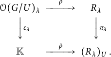
Since $\varepsilon _\lambda (f_\lambda ) = 1$
, we get
$\varepsilon _\lambda (f_\lambda ) = 1$
, we get $\bar \rho (1) = h$
and so
$\bar \rho (1) = h$
and so $\pi _\lambda (\Psi (f\otimes h)) = \pi _\lambda (\rho (f)) = \bar \rho (\varepsilon _\lambda (f))= \varepsilon _\lambda (f) h$
. This shows that the diagram
$\pi _\lambda (\Psi (f\otimes h)) = \pi _\lambda (\rho (f)) = \bar \rho (\varepsilon _\lambda (f))= \varepsilon _\lambda (f) h$
. This shows that the diagram

commutes.
3.3 Deformation of G-algebras
In 1980, the first author wrote a letter to Michel Brion [Reference Kraft18] in connection with his theses [Reference Brion5], explaining him a general method how to “reconstruct” a G-variety X from its U-invariants where G is a connected reductive group and $U \subset G$
a maximal unipotent subgroup. This method allows to show that certain properties of the U-invariants also hold for X (Proposition 3.16). At that time, Brion was interested in rational singularities, and he gave the proofs for this special case in his thesis, attributing them to Kraft.
$U \subset G$
a maximal unipotent subgroup. This method allows to show that certain properties of the U-invariants also hold for X (Proposition 3.16). At that time, Brion was interested in rational singularities, and he gave the proofs for this special case in his thesis, attributing them to Kraft.
In 1986, Popov reproved these results in [Reference Popov25] and added a statement about properties inherited by the U-invariants (see Remark 3.17). Later on, similar results appeared in the literature, e.g., in [Reference Grosshans11, Reference Vinberg29] where in both cases they were wrongly attributed to Popov.
We believe that our proofs are shorter and more transparent, and so we give them here, as an application of the methods developed above. The results are interesting in their own, but they will not be used in the remaining parts of the paper. We keep the assumption that G is semisimple, although it is not difficult to see that the results carry over to connected reductive groups.
Let R be a G-algebra with isotypic decomposition $R = \bigoplus _{\lambda \in \Lambda _{G}} R_{\lambda }$
. We define an isotypically graded G-algebra
$R = \bigoplus _{\lambda \in \Lambda _{G}} R_{\lambda }$
. We define an isotypically graded G-algebra $\operatorname {\mathrm {gr}} R$
in the following way. As a G-module, we set
$\operatorname {\mathrm {gr}} R$
in the following way. As a G-module, we set $\operatorname {\mathrm {gr}} R := R = \bigoplus _{\lambda \in \Lambda _{G}}R_{\lambda }$
, and the multiplication is defined by the symmetric bilinear map
$\operatorname {\mathrm {gr}} R := R = \bigoplus _{\lambda \in \Lambda _{G}}R_{\lambda }$
, and the multiplication is defined by the symmetric bilinear map
It is not difficult to see that this multiplication is associative, and hence defines a $\mathbb {K}$
-algebra structure on
$\mathbb {K}$
-algebra structure on $\operatorname {\mathrm {gr}} R$
such that
$\operatorname {\mathrm {gr}} R$
such that $\operatorname {\mathrm {gr}} R$
becomes an isotypically graded G-algebra. We now generalize Theorem 3.8 to general G-algebras.
$\operatorname {\mathrm {gr}} R$
becomes an isotypically graded G-algebra. We now generalize Theorem 3.8 to general G-algebras.
Proposition 3.12 For any G-algebra R, there is a canonical G-equivariant isomorphism of $\mathbb {K}$
-algebras
$\mathbb {K}$
-algebras
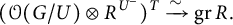 $$ \begin{align*}(\mathcal O(G/U)\otimes R^{U^{-}})^{T} \xrightarrow{\sim} \operatorname{\mathrm{gr}} R. \end{align*} $$
Proof The definition of the multiplication on $\operatorname {\mathrm {gr}} R$
implies that the subalgebra
$\operatorname {\mathrm {gr}} R$
implies that the subalgebra $(\operatorname {\mathrm {gr}} R)^{U^-}\subset \operatorname {\mathrm {gr}} R$
is equal to the subalgebra
$(\operatorname {\mathrm {gr}} R)^{U^-}\subset \operatorname {\mathrm {gr}} R$
is equal to the subalgebra $R^{U^-} \subset R$
since one has
$R^{U^-} \subset R$
since one has $R_\mu ^{U^-} \cdot R_\lambda ^{U^-} \subseteq R_{\mu +\lambda }^{U^-}$
. Applying Theorem 3.8 to the isotypically graded G-algebra
$R_\mu ^{U^-} \cdot R_\lambda ^{U^-} \subseteq R_{\mu +\lambda }^{U^-}$
. Applying Theorem 3.8 to the isotypically graded G-algebra $\operatorname {\mathrm {gr}} R$
, we get
$\operatorname {\mathrm {gr}} R$
, we get
 $$ \begin{align*}(\mathcal O(G/U)\otimes R^{U^{-}})^{T} = (\mathcal O(G/U)\otimes (\operatorname{\mathrm{gr}} R)^{U^{-}})^{T} \xrightarrow{\sim} \operatorname{\mathrm{gr}} R, \end{align*} $$
hence the claim.
The following Deformation Lemma shows that there exists a flat deformation of $\operatorname {\mathrm {gr}} R$
whose general fiber is R.
$\operatorname {\mathrm {gr}} R$
whose general fiber is R.
Lemma 3.13 Let R be a G-algebra. There exists a $\mathbb {K}[s]$
-algebra
$\mathbb {K}[s]$
-algebra $\tilde R$
with the following properties:
$\tilde R$
with the following properties:
-
(1)
$\tilde R$
is a free
$\mathbb {K}[s]$
-module and, in particular, flat over
$\mathbb {K}[s]$
. -
(2) There is an isomorphism
$\tilde R/ s\tilde R \simeq \operatorname {\mathrm {gr}} R$
as G-algebras. -
(3)
$\tilde R_s:=\mathbb {K}[s,s^{-1}]\otimes _{\mathbb {K}[s]} \tilde {R} \simeq \mathbb {K}[s,s^{-1}]\otimes _{\mathbb {K}} R$
.


Proof On $\Lambda _{G}$
, we have a partial ordering
$\Lambda _{G}$
, we have a partial ordering
 $$ \begin{align*}\mu \preceq \lambda :\!\!\iff \lambda - \mu \text{ is a sum of positive roots}, \end{align*} $$
which has the following property: if $V_\lambda , V_\mu $
are simple G-modules of highest weight
$V_\lambda , V_\mu $
are simple G-modules of highest weight $\lambda $
and
$\lambda $
and $\mu $
, then
$\mu $
, then $V_\lambda \otimes V_\mu = V_{\lambda + \mu } \oplus W$
where the simple summands of W have highest weights
$V_\lambda \otimes V_\mu = V_{\lambda + \mu } \oplus W$
where the simple summands of W have highest weights $\prec \lambda + \mu $
.
$\prec \lambda + \mu $
.
The cone ${\mathbb Q}_{\geq 0}\cdot \Phi _G^+ \subset {\mathbb Q}\otimes \Lambda _G$
generated by the positive roots
${\mathbb Q}_{\geq 0}\cdot \Phi _G^+ \subset {\mathbb Q}\otimes \Lambda _G$
generated by the positive roots $\Phi _G^+$
is pointed and contains
$\Phi _G^+$
is pointed and contains ${\mathbb Q}_{\geq 0}\cdot \Lambda _{G}$
. Therefore, we can find a
${\mathbb Q}_{\geq 0}\cdot \Lambda _{G}$
. Therefore, we can find a ${\mathbb Q}$
-linear function
${\mathbb Q}$
-linear function $p\colon {\mathbb Q}\otimes \Lambda _G \to {\mathbb Q}$
such that the following holds:
$p\colon {\mathbb Q}\otimes \Lambda _G \to {\mathbb Q}$
such that the following holds:
-
(1)
$p(\lambda )\in {\mathbb N}$
for all dominant weights
$\lambda \in \Lambda _G$
. -
(2)
$p(\alpha ) \in {\mathbb N}_{>0}$
for all positive roots
$\alpha \in \Phi _G^+$
.


In particular, if $\mu \prec \lambda $
, then
$\mu \prec \lambda $
, then $p(\mu )<p(\lambda )$
. Setting
$p(\mu )<p(\lambda )$
. Setting $R_n:=\bigoplus _{p(\lambda )\leq n} R_\lambda $
for
$R_n:=\bigoplus _{p(\lambda )\leq n} R_\lambda $
for $n\geq 0$
, we get
$n\geq 0$
, we get $R_n \cdot R_m\subseteq R_{n+m}$
. It follows that the G-stable subspace
$R_n \cdot R_m\subseteq R_{n+m}$
. It follows that the G-stable subspace
 $$ \begin{align*}\tilde R:=\textstyle{\bigoplus_{n\geq 0}} \mathbb{K} s^n \otimes R_n \subseteq \mathbb{K}[s]\otimes R \end{align*} $$
is a subalgebra containing $\mathbb {K}[s]$
. Since the isotypic component
$\mathbb {K}[s]$
. Since the isotypic component $\tilde R_\lambda $
is given by
$\tilde R_\lambda $
is given by
 $$ \begin{align*}\tilde R_\lambda = \textstyle{\bigoplus_{n\geq p(\lambda)}} \mathbb{K} s^n\otimes R_\lambda, \end{align*} $$
we see that $\tilde R$
is a free
$\tilde R$
is a free $\mathbb {K}[s]$
-module, proving (1). Moreover,
$\mathbb {K}[s]$
-module, proving (1). Moreover,
 $$ \begin{align*}s(\mathbb{K} s^n \otimes R_n) = \mathbb{K} s^{n+1}\otimes R_n \subseteq \mathbb{K} s^{n+1} \otimes R_{n+1}, \end{align*} $$
and hence $\tilde R / s \tilde R = \bigoplus _{n\geq 0} R_n/R_{n-1}$
where we set
$\tilde R / s \tilde R = \bigoplus _{n\geq 0} R_n/R_{n-1}$
where we set $R_{-1}=(0)$
. From the canonical decomposition
$R_{-1}=(0)$
. From the canonical decomposition $R_n = (\bigoplus _{p(\lambda )=n} R_\lambda ) \oplus R_{n-1}$
, we see that
$R_n = (\bigoplus _{p(\lambda )=n} R_\lambda ) \oplus R_{n-1}$
, we see that $\tilde R / s\tilde R = R = \operatorname {\mathrm {gr}} R$
as a G-module, and the multiplication of
$\tilde R / s\tilde R = R = \operatorname {\mathrm {gr}} R$
as a G-module, and the multiplication of $R_\lambda \subset R_n/R_{n-1}$
with
$R_\lambda \subset R_n/R_{n-1}$
with $R_\mu \subset R_m/R_{m-1}$
is given by the product in R followed by the projection onto
$R_\mu \subset R_m/R_{m-1}$
is given by the product in R followed by the projection onto $R_{n+m}/R_{n+m-1}$
. We have
$R_{n+m}/R_{n+m-1}$
. We have $R_\lambda \cdot R_\mu = V \oplus W$
, where
$R_\lambda \cdot R_\mu = V \oplus W$
, where $V \subseteq R_{\lambda +\mu }$
and all summands of W have highest weights
$V \subseteq R_{\lambda +\mu }$
and all summands of W have highest weights $\rho \prec \lambda + \mu $
. This implies that
$\rho \prec \lambda + \mu $
. This implies that $p(\rho ) < p(\lambda +\mu ) = n+m$
and so
$p(\rho ) < p(\lambda +\mu ) = n+m$
and so $W \subseteq R_{n+m-1}$
. Hence, the product of
$W \subseteq R_{n+m-1}$
. Hence, the product of $R_\lambda $
and
$R_\lambda $
and $R_\mu $
in
$R_\mu $
in $\tilde R / s\tilde R$
coincides with the product in
$\tilde R / s\tilde R$
coincides with the product in $\operatorname {\mathrm {gr}} R$
, proving (2).
$\operatorname {\mathrm {gr}} R$
, proving (2).
Finally, the subalgebra $\tilde R_s \subseteq \mathbb {K}[s,s^{-1}]\otimes R$
contains
$\tilde R_s \subseteq \mathbb {K}[s,s^{-1}]\otimes R$
contains $\mathbb {K} s^\ell \otimes R_n$
for all
$\mathbb {K} s^\ell \otimes R_n$
for all $\ell \in {\mathbb Z}$
and all
$\ell \in {\mathbb Z}$
and all $n\in {\mathbb N}$
, and hence is equal to
$n\in {\mathbb N}$
, and hence is equal to $\mathbb {K}[s,s^{-1}] \otimes R$
, proving the last claim (3).
$\mathbb {K}[s,s^{-1}] \otimes R$
, proving the last claim (3).
Remark 3.14 Let Z be a variety. For simplicity, we assume that Z is affine. Then a flat family $(A_z)_{z \in Z}$
of finitely generated
$(A_z)_{z \in Z}$
of finitely generated $\mathbb {K}$
-algebras is a finitely generated and flat
$\mathbb {K}$
-algebras is a finitely generated and flat $\mathcal O(Z)$
-algebra A such that
$\mathcal O(Z)$
-algebra A such that $A_z=A/\mathfrak {m}_z A$
where
$A_z=A/\mathfrak {m}_z A$
where $\mathfrak {m}_z$
is the maximal ideal of
$\mathfrak {m}_z$
is the maximal ideal of $z \in Z$
.
$z \in Z$
.
We say that a property $\mathcal P$
for finitely generated
$\mathcal P$
for finitely generated $\mathbb {K}$
-algebras is open if for any flat family
$\mathbb {K}$
-algebras is open if for any flat family $(A_z)_{z \in Z}$
of finitely generated
$(A_z)_{z \in Z}$
of finitely generated $\mathbb {K}$
-algebras the subset
$\mathbb {K}$
-algebras the subset $\{z \in Z\mid A_z \text { has property }\mathcal P\}$
is open in Z.
$\{z \in Z\mid A_z \text { has property }\mathcal P\}$
is open in Z.
The Deformation Lemma 3.13 tells us that for a given G-algebra R, there is a flat family $(R_z)_{z \in {\mathbb A}^1}$
of finitely generated G-algebras over the affine line
$(R_z)_{z \in {\mathbb A}^1}$
of finitely generated G-algebras over the affine line ${\mathbb A}^1$
such that
${\mathbb A}^1$
such that $R_0 \simeq \operatorname {\mathrm {gr}} R$
and
$R_0 \simeq \operatorname {\mathrm {gr}} R$
and $R_z \simeq R$
for all
$R_z \simeq R$
for all $z\in {\mathbb A}^1\setminus \{0\}$
. Together with Proposition 3.12, this allows to show that certain properties of the U-invariants
$z\in {\mathbb A}^1\setminus \{0\}$
. Together with Proposition 3.12, this allows to show that certain properties of the U-invariants $R^{U}$
also hold for R.
$R^{U}$
also hold for R.
Example 3.15 The following result is due to Vust [Reference Vust31, Section 1, Théorème 1]: if R is a finitely generated G-algebra such that $R^{U}$
is normal, then R is normal. In fact, since
$R^{U}$
is normal, then R is normal. In fact, since $R^{U^{-}} \simeq R^{U}$
and
$R^{U^{-}} \simeq R^{U}$
and $\mathcal O(G/U)$
are both normal, we see that
$\mathcal O(G/U)$
are both normal, we see that $(\mathcal O(G/U)\otimes R^{U^{-}})^{T}$
is normal, and hence
$(\mathcal O(G/U)\otimes R^{U^{-}})^{T}$
is normal, and hence $\operatorname {\mathrm {gr}} R$
is normal, by Proposition 3.12. Moreover, normality is an open property (see [Reference Grothendieck12, Corollaire 12.1.7(v)]). Since
$\operatorname {\mathrm {gr}} R$
is normal, by Proposition 3.12. Moreover, normality is an open property (see [Reference Grothendieck12, Corollaire 12.1.7(v)]). Since $\operatorname {\mathrm {gr}} R \simeq R_0$
is normal, the Deformation Lemma implies that
$\operatorname {\mathrm {gr}} R \simeq R_0$
is normal, the Deformation Lemma implies that $R_x$
is normal for all x in an open neighborhood W of
$R_x$
is normal for all x in an open neighborhood W of $0 \in {\mathbb A}^1$
; hence, R is normal.
$0 \in {\mathbb A}^1$
; hence, R is normal.
The argument from this example can be formalized in the following way.
Proposition 3.16 Let $\mathcal P$
be a property for finitely generated
$\mathcal P$
be a property for finitely generated $\mathbb {K}$
-algebras which satisfies the following conditions.
$\mathbb {K}$
-algebras which satisfies the following conditions.
-
(i)
$\mathcal P$
is open. -
(ii)
$\mathcal O(G/U)$
has property
$\mathcal P$
. -
(iii) If R and S have property
$\mathcal P$
, then so does
$R\otimes S$
. -
(iv) If R is a T-algebra with property
$\mathcal P$
, then
$R^{T}$
has property
$\mathcal P$
.


Then a finitely generated G-algebra R has property $\mathcal P$
if
$\mathcal P$
if $R^{U}$
has property
$R^{U}$
has property $\mathcal P$
.
$\mathcal P$
.
Proof If $R^U$
has property
$R^U$
has property $\mathcal P$
, then so does
$\mathcal P$
, then so does $R^{U^-}$
. Hence, assumptions (ii)–(vi) imply that
$R^{U^-}$
. Hence, assumptions (ii)–(vi) imply that $(\mathcal O(G/U)\otimes R^{U^-})^T$
has property
$(\mathcal O(G/U)\otimes R^{U^-})^T$
has property $\mathcal P$
. In particular,
$\mathcal P$
. In particular, $\operatorname {\mathrm {gr}} R$
has property
$\operatorname {\mathrm {gr}} R$
has property $\mathcal P$
by Proposition 3.12. Now, (i) implies that R has property
$\mathcal P$
by Proposition 3.12. Now, (i) implies that R has property $\mathcal P$
as well.
$\mathcal P$
as well.
A very interesting property satisfying the assumption of the proposition above is that of rational singularities (see [Reference Boutot4]).
Remark 3.17 Let X be a G-variety, and consider the action of $G \times U$
on
$G \times U$
on $G \times X$
given by
$G \times X$
given by $h(g,x) := (hg,hx)$
and
$h(g,x) := (hg,hx)$
and $u(g,x):=(gu^{-1},x)$
. Then
$u(g,x):=(gu^{-1},x)$
. Then
 $$ \begin{align*}(G \times X)/\!\!/ (G\times U) \simeq G/\!\!/ U\star^G X \simeq X/\!\!/ U. \end{align*} $$
In particular, $(\mathcal O(G/U)\otimes \mathcal O(X))^G \simeq \mathcal O(X)^U$
. In fact, the isomorphism
$(\mathcal O(G/U)\otimes \mathcal O(X))^G \simeq \mathcal O(X)^U$
. In fact, the isomorphism $G \times X \xrightarrow {\sim } G\times X$
,
$G \times X \xrightarrow {\sim } G\times X$
, $(g,x)\mapsto (g,g^{-1} x)$
is
$(g,x)\mapsto (g,g^{-1} x)$
is $G \times U$
-equivariant for the action
$G \times U$
-equivariant for the action $u\cdot (g,x) := (gu^{-1},ux)$
and
$u\cdot (g,x) := (gu^{-1},ux)$
and $h\cdot (g,x) := (hg,x)$
on the right-hand side, and the claim follows.
$h\cdot (g,x) := (hg,x)$
on the right-hand side, and the claim follows.
This formula gives the following result (cf. [Reference Popov25]). Assume that a property $\mathcal P$
for finitely generated
$\mathcal P$
for finitely generated $\mathbb {K}$
-algebra satisfies the following conditions.
$\mathbb {K}$
-algebra satisfies the following conditions.
-
(i)
$\mathcal O(G/U)$
has property
$\mathcal P$
. -
(ii) If R and S have property
$\mathcal P$
, then so does
$R\otimes S$
. -
(iii) If R is a G-algebra with property
$\mathcal P$
, then
$R^{G}$
has property
$\mathcal P$
.


Then $R^U$
has property
$R^U$
has property $\mathcal P$
if R does.
$\mathcal P$
if R does.
4 Small G-varieties
Recall that an affine G-variety is small if every nontrivial orbit is a minimal orbit. We will show that the coordinate ring of a small G-variety is an isotypically graded G-algebra and then use the results of the previous section to obtain important properties of small G-varieties and a classification.
Remark 4.1 The G-action on a small G-variety X is fix-pointed, which means that the closed orbits are fixed points. This has some interesting consequences. For example, it is not difficult to see that for a fix-pointed action of a reductive group on an affine variety X, the algebraic quotient $\pi \colon X \to X/\!\!/ G$
induces an isomorphism
$\pi \colon X \to X/\!\!/ G$
induces an isomorphism $X^G \xrightarrow {\sim } X/\!\!/ G$
(cf. [Reference Bass and Haboush1, Section 10, p. 475]).
$X^G \xrightarrow {\sim } X/\!\!/ G$
(cf. [Reference Bass and Haboush1, Section 10, p. 475]).
4.1 A geometric formulation
We first translate Theorem 3.8 into the geometric setting. By a result of Hadziev [Reference Hadžiev13] (cf. [Reference Kraft19, Lemma 3.2]), the U-invariants $\mathcal O(G)^{U}$
are finitely generated, and hence define an affine G-variety
$\mathcal O(G)^{U}$
are finitely generated, and hence define an affine G-variety $G/\!\!/ U$
with a G-equivariant quotient map
$G/\!\!/ U$
with a G-equivariant quotient map $\eta \colon G \to G/\!\!/ U$
. Since
$\eta \colon G \to G/\!\!/ U$
. Since $\mathcal O(G/U) = \mathcal O(G)^U = \mathcal O(G/\!\!/ U)$
, the canonical G-equivariant map
$\mathcal O(G/U) = \mathcal O(G)^U = \mathcal O(G/\!\!/ U)$
, the canonical G-equivariant map $G/U \to G/\!\!/ U$
,
$G/U \to G/\!\!/ U$
, $g U\mapsto \eta (g)$
, is birational, hence an open immersion:
$g U\mapsto \eta (g)$
, is birational, hence an open immersion: $G/U = G\eta (e) \subset G/\!\!/ U$
. Moreover, the T-action on
$G/U = G\eta (e) \subset G/\!\!/ U$
. Moreover, the T-action on $G/U$
by right multiplication extends to a T-action on
$G/U$
by right multiplication extends to a T-action on $G/\!\!/ U$
commuting with the G-action.
$G/\!\!/ U$
commuting with the G-action.
For an affine G-variety X, we have a canonical G-equivariant morphism
 $$\begin{align*}G/U \times X^{U} \to X,\quad (g U,x) \mapsto g x, \end{align*}$$
and a T-action on $G/U \times X^{U}$
given by
$G/U \times X^{U}$
given by $(t,(g U,x))\mapsto (g t^{-1} U, t x)$
. As
$(t,(g U,x))\mapsto (g t^{-1} U, t x)$
. As $\mathcal O(G/U \times X^{U}) = \mathcal O(G/U) \otimes \mathcal O(X^{U}) = \mathcal O(G/\!\!/ U) \otimes \mathcal O(X^{U}) = \mathcal O(G/\!\!/ U \times X^{U})$
(see [Reference Demazure and Gabriel6, Chapter I, Section 2, Proposition 2.6]), they, respectively, extend to a morphism
$\mathcal O(G/U \times X^{U}) = \mathcal O(G/U) \otimes \mathcal O(X^{U}) = \mathcal O(G/\!\!/ U) \otimes \mathcal O(X^{U}) = \mathcal O(G/\!\!/ U \times X^{U})$
(see [Reference Demazure and Gabriel6, Chapter I, Section 2, Proposition 2.6]), they, respectively, extend to a morphism $\varphi \colon G/\!\!/ U\times X^{U} \to X$
and a T-action on
$\varphi \colon G/\!\!/ U\times X^{U} \to X$
and a T-action on $G/\!\!/ U\times X^{U}$
. It follows that
$G/\!\!/ U\times X^{U}$
. It follows that $\varphi $
is constant on the T-orbits, and thus induces a G-equivariant morphism
$\varphi $
is constant on the T-orbits, and thus induces a G-equivariant morphism
 $$ \begin{align*}\Phi \colon G/\!\!/ U \star^{T} X^{U} :=(G/\!\!/ U \times X^{U})/\!\!/ T \to X. \end{align*} $$
Proposition 4.2 Let X be an affine G-variety, and assume that $\mathcal O(X)$
is an isotypically graded G-algebra. Then the canonical morphism
$\mathcal O(X)$
is an isotypically graded G-algebra. Then the canonical morphism
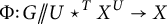 $$ \begin{align*}\Phi \colon G/\!\!/ U \star^{T} X^{U} \to X \end{align*} $$
is a G-equivariant isomorphism. Its comorphism is the inverse of the isomorphism $\Psi $
from Theorem 3.8.
$\Psi $
from Theorem 3.8.
Proof By definition, the comorphism $\Phi ^{*}\colon \mathcal O(X) \longrightarrow (\mathcal O(G/U)\otimes \mathcal O(X^{U}))^{T}$
is given as follows: if
$\Phi ^{*}\colon \mathcal O(X) \longrightarrow (\mathcal O(G/U)\otimes \mathcal O(X^{U}))^{T}$
is given as follows: if $\Phi ^{*}(f) = \sum _{j} f_{j}\otimes h_{j}$
, then
$\Phi ^{*}(f) = \sum _{j} f_{j}\otimes h_{j}$
, then $\Phi ^{*}(f)(g U,x)=f(g x) = \sum _{j}f_{j}(g U) h_{j}(x)$
. Consider the evaluation map
$\Phi ^{*}(f)(g U,x)=f(g x) = \sum _{j}f_{j}(g U) h_{j}(x)$
. Consider the evaluation map $\varepsilon \colon \mathcal O(G/U)\to \mathbb {K}$
,
$\varepsilon \colon \mathcal O(G/U)\to \mathbb {K}$
, $f\mapsto f(e U)$
. Then
$f\mapsto f(e U)$
. Then $f(x)=\sum _{j}\varepsilon (f_{j})h_{j}(x)$
for all
$f(x)=\sum _{j}\varepsilon (f_{j})h_{j}(x)$
for all $x\in X^U$
, which shows that the diagram
$x\in X^U$
, which shows that the diagram

commutes, where $\rho $
is the restriction map, i.e.,
$\rho $
is the restriction map, i.e., $\rho (f) = \sum _{j}\varepsilon (f_{j})h_{j} = (\varepsilon \otimes \operatorname {\mathrm {id}})(\Phi ^{*}(f))$
. Since
$\rho (f) = \sum _{j}\varepsilon (f_{j})h_{j} = (\varepsilon \otimes \operatorname {\mathrm {id}})(\Phi ^{*}(f))$
. Since $\mathcal O(X)$
is an isotypically graded G-algebra, it follows from Remark 3.4 that the restriction map
$\mathcal O(X)$
is an isotypically graded G-algebra, it follows from Remark 3.4 that the restriction map $\rho $
is equal to the universal U-projection
$\rho $
is equal to the universal U-projection $\pi _{U}\colon \mathcal O(X) \to \mathcal O(X)_{U}$
. If we show that
$\pi _{U}\colon \mathcal O(X) \to \mathcal O(X)_{U}$
. If we show that $\varepsilon \otimes \operatorname {\mathrm {id}}$
is also equal to the U-projection
$\varepsilon \otimes \operatorname {\mathrm {id}}$
is also equal to the U-projection ${\pi }_U\colon (\mathcal O(G/U)\otimes \mathcal O(X^{U}))^{T}\to \left ((\mathcal O(G/U)\otimes \mathcal O(X^{U}))^{T}\right )_U$
, then
${\pi }_U\colon (\mathcal O(G/U)\otimes \mathcal O(X^{U}))^{T}\to \left ((\mathcal O(G/U)\otimes \mathcal O(X^{U}))^{T}\right )_U$
, then $\Phi ^*$
is an isomorphism by Lemma 3.5. We have
$\Phi ^*$
is an isomorphism by Lemma 3.5. We have
 $$ \begin{align*}(\mathcal O(G/U)\otimes \mathcal O(X^{U}))^{T} = \textstyle \bigoplus_{\lambda\in\Lambda_G}\mathcal O(G/U)_\lambda \otimes \mathcal O(X^U)_{[-\lambda^\vee]}, \end{align*} $$
where $ \mathcal O(X^U)_{[\mu ]}$
is the T-weight space of
$ \mathcal O(X^U)_{[\mu ]}$
is the T-weight space of $\mathcal O(X^U)$
of weight
$\mathcal O(X^U)$
of weight $\mu $
. Since the evaluation map
$\mu $
. Since the evaluation map $\varepsilon _\lambda \colon \mathcal O(G/U)_\lambda \to \mathbb {K}$
,
$\varepsilon _\lambda \colon \mathcal O(G/U)_\lambda \to \mathbb {K}$
, $f\mapsto f(e U)$
, is the universal U-projection (Lemma 3.7), we see that the linear map
$f\mapsto f(e U)$
, is the universal U-projection (Lemma 3.7), we see that the linear map $\mathcal O(G/U)_\lambda \otimes \mathcal O(X^U)_{[-\lambda ^\vee ]} \to \mathcal O(X^U)_{[-\lambda ^\vee ]}$
,
$\mathcal O(G/U)_\lambda \otimes \mathcal O(X^U)_{[-\lambda ^\vee ]} \to \mathcal O(X^U)_{[-\lambda ^\vee ]}$
, $\sum _j f_j\otimes h_j \mapsto \sum _j\varepsilon (f_j)h_j$
, is the U-projection as well, and the claim follows.
$\sum _j f_j\otimes h_j \mapsto \sum _j\varepsilon (f_j)h_j$
, is the U-projection as well, and the claim follows.
It remains to see that $\Phi ^*$
is equal to the inverse of
$\Phi ^*$
is equal to the inverse of $\Psi $
from Theorem 3.8. Using again Lemma 3.5, it suffices to show that the diagram
$\Psi $
from Theorem 3.8. Using again Lemma 3.5, it suffices to show that the diagram

commutes. This is stated in Remark 3.11.
4.2 The structure of small G-varieties
Proposition 4.3 Let X be an irreducible small G-variety. Then the following holds.
-
(1) The G-action is fix-pointed, and all minimal orbits in X have the same type
$\lambda $
. -
(2)
$\mathcal O(X)$
is an isotypically graded G-algebra of type
$\lambda ^{\!\vee }$
. -
(3) The quotient
$X\to X/\!\!/ U^-$
restricts to an isomorphism
$X^U\xrightarrow {\sim } X/\!\!/ U^-$
. Moreover,
$$ \begin{align*}X \text{ normal } \iff X^U \text{ normal } \iff X/\!\!/ U \text{ normal.} \end{align*} $$


We call such a variety X a small G-variety of type $\lambda $
.
$\lambda $
.
Proof (1) By hypothesis, any nontrivial orbit $O \subset X$
is minimal, so
$O \subset X$
is minimal, so $\overline {O}=O\cup \{x_{0}\}$
, where
$\overline {O}=O\cup \{x_{0}\}$
, where $x_{0}\in X^{G}$
by Proposition 2.11(1). In particular, the G-action is fix-pointed.
$x_{0}\in X^{G}$
by Proposition 2.11(1). In particular, the G-action is fix-pointed.
We can assume that X is a closed G-stable subvariety of a G-module W (see, for example, [Reference Kraft20, Corollary 2.3.5]). Let $O \subset X$
be a nontrivial orbit. There is a linear projection
$O \subset X$
be a nontrivial orbit. There is a linear projection $p\colon W \to V$
onto a simple G-module V of highest weight
$p\colon W \to V$
onto a simple G-module V of highest weight $\lambda $
such that
$\lambda $
such that $O \nsubseteq \ker p$
. Proposition 2.11(2) implies that
$O \nsubseteq \ker p$
. Proposition 2.11(2) implies that $p(O) = O_{\lambda }$
and that O is of the same type as
$p(O) = O_{\lambda }$
and that O is of the same type as $O_{\lambda }$
. The same is true for all orbits
$O_{\lambda }$
. The same is true for all orbits $O'$
from the open subset
$O'$
from the open subset $X':= X \setminus \ker p$
of X. Since X is irreducible, all minimal orbits are of type
$X':= X \setminus \ker p$
of X. Since X is irreducible, all minimal orbits are of type $\lambda $
. It follows from Example 3.1 that
$\lambda $
. It follows from Example 3.1 that $\mathcal O(O)$
is of type
$\mathcal O(O)$
is of type $\lambda ^\vee $
.
$\lambda ^\vee $
.
(2) Since X is small, we have $X = G\cdot X^U$
, showing that the morphism
$X = G\cdot X^U$
, showing that the morphism $G/U \times X^U \to X$
is surjective. Thus, we obtain a G-equivariant inclusion
$G/U \times X^U \to X$
is surjective. Thus, we obtain a G-equivariant inclusion $\mathcal O(X) \hookrightarrow \mathcal O(G/U) \otimes \mathcal O(X^U)$
where the G-algebra on the right is isotypically graded (by (*) and Example 3.1). Hence, it follows from (1) that
$\mathcal O(X) \hookrightarrow \mathcal O(G/U) \otimes \mathcal O(X^U)$
where the G-algebra on the right is isotypically graded (by (*) and Example 3.1). Hence, it follows from (1) that $\mathcal O(X)$
is isotypically graded of type
$\mathcal O(X)$
is isotypically graded of type $\lambda ^\vee $
.
$\lambda ^\vee $
.
(3) The first part follows from Remark 3.4. It also shows that if X is normal, then $X^U$
is normal. The other implication follows from the isomorphism
$X^U$
is normal. The other implication follows from the isomorphism $\Phi $
in Proposition 4.2 because
$\Phi $
in Proposition 4.2 because $G/\!\!/ U$
is normal (cf. Example 3.15). The second equivalence is clear.
$G/\!\!/ U$
is normal (cf. Example 3.15). The second equivalence is clear.
Proposition 4.4 Let X be an irreducible small G-variety of type $\lambda $
.
$\lambda $
.
-
(1) There is a unique
${\mathbb {K}^{*}}$
-action on X which induces the canonical
${\mathbb {K}^{*}}$
-action on each minimal orbit and commutes with the G-action. This action on
$X^{U}$
is fix-pointed, and we get isomorphisms
$X^{U}/\!\!/{\mathbb {K}^{*}} \xrightarrow {\sim } X/\!\!/ G \xleftarrow {\sim } X^{G}$
. -
(2) The morphism
$G\times X^U \to X$
,
$(g,x)\mapsto g x$
, induces a G-equivariant isomorphism where
$$\begin{align*}\Phi\colon\overline{O_{\lambda}}\star^{{\mathbb{K}^{*}}} X^{U}\xrightarrow{\sim} X, \end{align*}$$
${\mathbb {K}^{*}}$
acts on
$\overline {O_{\lambda }}$
by the inverse of the scalar multiplication:
$(t,x)\mapsto t^{-1}\cdot x$
.
-
(3) We have
$\operatorname {\mathrm {Norm}}_{G}(X^{U})=P_{\lambda }$
, and the G-equivariant morphism is proper, surjective, and birational, and it induces an isomorphism between the algebras of regular functions.
$$\begin{align*}\Theta\colon G\times^{P_{\lambda}}X^{U}\rightarrow X,\quad [g,x]\mapsto g x, \end{align*}$$


Proof (1) By Proposition 4.3(2), $\mathcal O(X)$
is an isotypically graded G-algebra of type
$\mathcal O(X)$
is an isotypically graded G-algebra of type $\lambda ^{\vee }$
. If we define the
$\lambda ^{\vee }$
. If we define the ${\mathbb {K}^{*}}$
-action on
${\mathbb {K}^{*}}$
-action on $\mathcal O(X)$
such that the isotypic component of type
$\mathcal O(X)$
such that the isotypic component of type $n \lambda ^{\vee }$
has weight
$n \lambda ^{\vee }$
has weight $-n$
, then this action is fix-pointed and restricts to the canonical
$-n$
, then this action is fix-pointed and restricts to the canonical ${\mathbb {K}^{*}}$
-action on the closure of each minimal orbit (Proposition 2.14(3)). Since X is the union of the closures of the minimal orbits, this
${\mathbb {K}^{*}}$
-action on the closure of each minimal orbit (Proposition 2.14(3)). Since X is the union of the closures of the minimal orbits, this ${\mathbb {K}^{*}}$
-action is unique and commutes with the G-action. We have
${\mathbb {K}^{*}}$
-action is unique and commutes with the G-action. We have $X^G= (X^U)^{{\mathbb {K}^{*}}}$
and the
$X^G= (X^U)^{{\mathbb {K}^{*}}}$
and the ${\mathbb {K}^{*}}$
-action on
${\mathbb {K}^{*}}$
-action on $X^U$
is fix-pointed, since this holds for the closure of a minimal orbit. This implies that
$X^U$
is fix-pointed, since this holds for the closure of a minimal orbit. This implies that $X^G = (X^U)^{{\mathbb {K}^{*}}} \xrightarrow {\sim } X^U/\!\!/ {\mathbb {K}^{*}}$
, and
$X^G = (X^U)^{{\mathbb {K}^{*}}} \xrightarrow {\sim } X^U/\!\!/ {\mathbb {K}^{*}}$
, and $X^G \xrightarrow {\sim } X/\!\!/ G$
since the G-action is fix-pointed, which yields the remaining claims.
$X^G \xrightarrow {\sim } X/\!\!/ G$
since the G-action is fix-pointed, which yields the remaining claims.
(2) Choose $x_{0} \in O_{\lambda }^{U}$
and consider the G-equivariant morphism
$x_{0} \in O_{\lambda }^{U}$
and consider the G-equivariant morphism $\eta \colon G/\!\!/ U \to \overline {O_{\lambda }}$
induced by
$\eta \colon G/\!\!/ U \to \overline {O_{\lambda }}$
induced by $g U\mapsto g x_0$
. For
$g U\mapsto g x_0$
. For $t \in T$
, we get
$t \in T$
, we get $\eta (gt^{-1}U) = gt^{-1}x_0 = \lambda (t)^{-1}\cdot gx_0$
. This shows that the T-action on
$\eta (gt^{-1}U) = gt^{-1}x_0 = \lambda (t)^{-1}\cdot gx_0$
. This shows that the T-action on $G/\!\!/ U$
by right multiplication induces a T-action on
$G/\!\!/ U$
by right multiplication induces a T-action on $\overline {O_{\lambda }}$
which factors through
$\overline {O_{\lambda }}$
which factors through $\lambda \colon T \to {\mathbb {K}^{*}}$
, and the induced
$\lambda \colon T \to {\mathbb {K}^{*}}$
, and the induced ${\mathbb {K}^{*}}$
-action is the inverse of the scalar multiplication, i.e., the inverse of the canonical
${\mathbb {K}^{*}}$
-action is the inverse of the scalar multiplication, i.e., the inverse of the canonical ${\mathbb {K}^{*}}$
-action.
${\mathbb {K}^{*}}$
-action.
Define $D:=\ker \lambda \subset T$
. We claim that
$D:=\ker \lambda \subset T$
. We claim that $\eta $
is the algebraic quotient under the action of D. In fact, the action of
$\eta $
is the algebraic quotient under the action of D. In fact, the action of $t\in T$
on
$t\in T$
on $\mathcal O(G/U)_\mu $
is by scalar multiplication with
$\mathcal O(G/U)_\mu $
is by scalar multiplication with $\mu ^\vee (t)$
(Remark 3.6(1)). Hence, the action of D is trivial if and only if
$\mu ^\vee (t)$
(Remark 3.6(1)). Hence, the action of D is trivial if and only if $\mu $
is a multiple of
$\mu $
is a multiple of $\lambda ^{\!\vee }$
. This implies that
$\lambda ^{\!\vee }$
. This implies that
 $$ \begin{align*}\mathcal O(G/U)^{D} = \textstyle\bigoplus_{\mu\in\Lambda_G} \mathcal O(G/U)_\mu^D = \bigoplus_{k\geq 0} V_{k\lambda^\vee} \simeq \mathcal O(\overline{O_{\lambda}}) \end{align*} $$
(see Lemma 2.2(2)). Since X is of type $\lambda $
, it follows that
$\lambda $
, it follows that $D = \ker \lambda $
acts trivially on
$D = \ker \lambda $
acts trivially on $X^U$
. Therefore,
$X^U$
. Therefore, $(G/\!\!/ U \times X^U)/\!\!/ D = \overline {O_{\lambda }}\times X^U$
, and so
$(G/\!\!/ U \times X^U)/\!\!/ D = \overline {O_{\lambda }}\times X^U$
, and so
 $$ \begin{align*}G/\!\!/ U \star^T X^U = (G/\!\!/ U \star^D X^U)/\!\!/ T = (\overline{O_{\lambda}}\times X^U)/\!\!/ T. \end{align*} $$
By construction, the T-action on $\overline {O_{\lambda }}\times X^U$
is given by
$\overline {O_{\lambda }}\times X^U$
is given by $t(v,x)= (\lambda (t)^{-1}\cdot v, t x)$
, i.e., by the inverse of the canonical
$t(v,x)= (\lambda (t)^{-1}\cdot v, t x)$
, i.e., by the inverse of the canonical ${\mathbb {K}^{*}}$
-action on
${\mathbb {K}^{*}}$
-action on $\overline {O_{\lambda }}$
and the given action on
$\overline {O_{\lambda }}$
and the given action on $X^U$
. Hence,
$X^U$
. Hence, $ (\overline {O_{\lambda }}\times X^U)/\!\!/ T = \overline {O_{\lambda }} \star ^{{\mathbb {K}^{*}}} X^U$
, and the claim follows from Proposition 4.2.
$ (\overline {O_{\lambda }}\times X^U)/\!\!/ T = \overline {O_{\lambda }} \star ^{{\mathbb {K}^{*}}} X^U$
, and the claim follows from Proposition 4.2.
(3) Consider the action of $P_{\lambda }$
on
$P_{\lambda }$
on $G \times X^{U}$
given by
$G \times X^{U}$
given by $p(g,x) = (g p^{-1},p x)$
. Then the action map
$p(g,x) = (g p^{-1},p x)$
. Then the action map $G \times X^{U}\to X$
,
$G \times X^{U}\to X$
, $(g,x)\mapsto g x$
, factors through the geometric quotient
$(g,x)\mapsto g x$
, factors through the geometric quotient
 $$ \begin{align*} G\times^{P_{\lambda}}X^{U}:=(G\times X^{U})/ P_{\lambda}. \end{align*} $$
For $\Theta $
, we have the following factorization:
$\Theta $
, we have the following factorization:
where the first map is a closed immersion and the second an isomorphism. Since $G/P_{\lambda }$
is complete, it follows that
$G/P_{\lambda }$
is complete, it follows that $\Theta $
is proper. Moreover,
$\Theta $
is proper. Moreover, $\Theta $
is surjective because every G-orbit meets
$\Theta $
is surjective because every G-orbit meets $X^{U}$
. We claim that
$X^{U}$
. We claim that $\Theta $
induces a bijection
$\Theta $
induces a bijection $G\times ^{P_{\lambda }}(X^{U}\setminus X^{G}) \to X\setminus X^{G}$
, which implies that
$G\times ^{P_{\lambda }}(X^{U}\setminus X^{G}) \to X\setminus X^{G}$
, which implies that $\Theta $
is birational. Indeed, if
$\Theta $
is birational. Indeed, if $x\in X^{U}\setminus X^{G}$
, then
$x\in X^{U}\setminus X^{G}$
, then $x \in O^{U}$
for a minimal orbit
$x \in O^{U}$
for a minimal orbit $O \subset X$
. If
$O \subset X$
. If $g x = g' x'$
for some
$g x = g' x'$
for some $x'\in X^{U}$
,
$x'\in X^{U}$
, $g'\in G$
, then
$g'\in G$
, then $x'\in O^{U}$
, and hence
$x'\in O^{U}$
, and hence $x' = q x$
for some
$x' = q x$
for some $q \in P_{\lambda }$
because the action of
$q \in P_{\lambda }$
because the action of $P_{\lambda }$
on
$P_{\lambda }$
on $O^{U}$
is transitive. It follows that
$O^{U}$
is transitive. It follows that $g^{-1}g' q\in G_{x}\subset P_{\lambda }$
, and hence
$g^{-1}g' q\in G_{x}\subset P_{\lambda }$
, and hence $p:=g^{-1} g'\in P_{\lambda }$
. Thus,
$p:=g^{-1} g'\in P_{\lambda }$
. Thus, $[g',x']=[g p,x']=[g,p x'] = [g,x]$
.
$[g',x']=[g p,x']=[g,p x'] = [g,x]$
.
It remains to see that the comorphism of $\Theta $
is an isomorphism on the global functions. Let
$\Theta $
is an isomorphism on the global functions. Let $K_{\lambda }$
be the kernel of the character
$K_{\lambda }$
be the kernel of the character $\lambda \colon P_{\lambda }\to {\mathbb {K}^{*}}$
. Then
$\lambda \colon P_{\lambda }\to {\mathbb {K}^{*}}$
. Then $G/K_\lambda \simeq O_\lambda $
, and the action of
$G/K_\lambda \simeq O_\lambda $
, and the action of $P_{\lambda }$
on G by right multiplication induces an action of
$P_{\lambda }$
on G by right multiplication induces an action of ${\mathbb {K}^{*}} = P_{\lambda }/K_{\lambda }$
on
${\mathbb {K}^{*}} = P_{\lambda }/K_{\lambda }$
on $G/K_{\lambda }$
by right multiplication corresponding to the canonical action on
$G/K_{\lambda }$
by right multiplication corresponding to the canonical action on $O_\lambda $
. This gives the G-equivariant isomorphisms
$O_\lambda $
. This gives the G-equivariant isomorphisms
 $$\begin{align*}G\times^{P_{\lambda}}X^{U} \xrightarrow{\sim} G/K_{\lambda}\star^{{\mathbb{K}^{*}}} X^{U} \xrightarrow{\sim} O_\lambda \star^{{\mathbb{K}^{*}}} X^U, \end{align*}$$
and the claim follows from (2).
Example 4.5 Let $X:=\overline {O_{\mu }} \subset V_{\mu }$
be the closure of the minimal orbit in
$X:=\overline {O_{\mu }} \subset V_{\mu }$
be the closure of the minimal orbit in $V_{\mu }$
, and let
$V_{\mu }$
, and let $\mu =\ell \lambda $
, where
$\mu =\ell \lambda $
, where $\lambda $
is indivisible. Then
$\lambda $
is indivisible. Then $X^{U}=\mathbb {K}$
, and from Proposition 4.4(2), we get an isomorphism
$X^{U}=\mathbb {K}$
, and from Proposition 4.4(2), we get an isomorphism
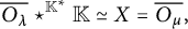 $$ \begin{align*}\overline{O_{\lambda}} \star^{{\mathbb{K}^{*}}} \mathbb{K} \simeq X = \overline{O_{\mu}}, \end{align*} $$
where ${\mathbb {K}^{*}}$
acts on
${\mathbb {K}^{*}}$
acts on $\overline {O_{\lambda }}$
by the inverse of the canonical action,
$\overline {O_{\lambda }}$
by the inverse of the canonical action, $(t,x)\mapsto t^{-1}\cdot x$
, and by the canonical action on
$(t,x)\mapsto t^{-1}\cdot x$
, and by the canonical action on $\mathbb {K} = \overline {O_\mu }$
, which is the scalar multiplication with
$\mathbb {K} = \overline {O_\mu }$
, which is the scalar multiplication with $\mu (t)$
.
$\mu (t)$
.
The second statement of Proposition 4.4 says that a small G-variety X can be reconstructed from the ${\mathbb {K}^{*}}$
-variety
${\mathbb {K}^{*}}$
-variety $X^U$
. In order to give a more precise statement, we introduce the following notion. A
$X^U$
. In order to give a more precise statement, we introduce the following notion. A ${\mathbb {K}^{*}}$
-action on an affine variety Y is called positively fix-pointed if for every
${\mathbb {K}^{*}}$
-action on an affine variety Y is called positively fix-pointed if for every $y \in Y$
the limit
$y \in Y$
the limit $\lim _{t\to 0}t y$
exists and is therefore a fixed point.
$\lim _{t\to 0}t y$
exists and is therefore a fixed point.
For a fix-pointed ${\mathbb {K}^{*}}$
-action on an irreducible affine variety Y, either the action is positively fix-pointed or the inverse action
${\mathbb {K}^{*}}$
-action on an irreducible affine variety Y, either the action is positively fix-pointed or the inverse action $(t,y)\mapsto t^{-1}y$
is positively fix-pointed. Indeed, for any
$(t,y)\mapsto t^{-1}y$
is positively fix-pointed. Indeed, for any $y \in Y$
, either
$y \in Y$
, either $\lim _{t\to 0}t y$
or
$\lim _{t\to 0}t y$
or $\lim _{t\to \infty }t y$
exists. Embedding Y equivariantly into a
$\lim _{t\to \infty }t y$
exists. Embedding Y equivariantly into a ${\mathbb {K}^{*}}$
-module, one sees that the subsets
${\mathbb {K}^{*}}$
-module, one sees that the subsets $Y_+:=\{y\in Y\mid \lim _{t\to 0}t y \text { exists}\}$
and
$Y_+:=\{y\in Y\mid \lim _{t\to 0}t y \text { exists}\}$
and $Y_-:=\{y\in Y\mid \lim _{t\to \infty }t y \text { exists}\}$
are closed. As Y is irreducible, this yields the claim. (The claim does not hold for connected
$Y_-:=\{y\in Y\mid \lim _{t\to \infty }t y \text { exists}\}$
are closed. As Y is irreducible, this yields the claim. (The claim does not hold for connected ${\mathbb {K}^{*}}$
-varieties, as the example of the union of the coordinate lines in the two-dimensional representation
${\mathbb {K}^{*}}$
-varieties, as the example of the union of the coordinate lines in the two-dimensional representation $t(x,y):=(t x,t^{-1} y)$
shows.)
$t(x,y):=(t x,t^{-1} y)$
shows.)
Remark 4.6 A positively fix-pointed ${\mathbb {K}^{*}}$
-action on Y extends to an action of the multiplicative semigroup
${\mathbb {K}^{*}}$
-action on Y extends to an action of the multiplicative semigroup $(\mathbb {K},\cdot )$
, and the morphism
$(\mathbb {K},\cdot )$
, and the morphism $\mathbb {K} \times Y \to Y$
,
$\mathbb {K} \times Y \to Y$
, $(s,y)\mapsto s y$
, induces an isomorphism
$(s,y)\mapsto s y$
, induces an isomorphism $\mathbb {K} \star ^{{\mathbb {K}^{*}}} Y \xrightarrow {\sim } Y$
. This follows from the commutative diagram
$\mathbb {K} \star ^{{\mathbb {K}^{*}}} Y \xrightarrow {\sim } Y$
. This follows from the commutative diagram
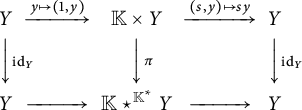
where the compositions of the horizontal maps are the identity.
Lemma 4.7 Let Y be a positively fix-pointed affine ${\mathbb {K}^{*}}$
-variety, and let
${\mathbb {K}^{*}}$
-variety, and let $\lambda \in \Lambda _G$
be indivisible. Consider the
$\lambda \in \Lambda _G$
be indivisible. Consider the ${\mathbb {K}^{*}}$
-action on
${\mathbb {K}^{*}}$
-action on $\overline {O_{\lambda }}\times Y$
given by
$\overline {O_{\lambda }}\times Y$
given by $t(v,y):=(t^{-1}\cdot v, t y)$
. Then
$t(v,y):=(t^{-1}\cdot v, t y)$
. Then
 $$ \begin{align*}X:=\overline{O_{\lambda}}\star^{{\mathbb{K}^{*}}}Y=(\overline{O_{\lambda}} \times Y)/\!\!/{\mathbb{K}^{*}} \end{align*} $$
is a small G-variety of type $\lambda $
where the action of G is induced by the action on
$\lambda $
where the action of G is induced by the action on $\overline {O_{\lambda }}$
. Moreover, there is canonical
$\overline {O_{\lambda }}$
. Moreover, there is canonical ${\mathbb {K}^{*}}$
-equivariant isomorphism
${\mathbb {K}^{*}}$
-equivariant isomorphism $X^{U}\xrightarrow {\sim } Y$
.
$X^{U}\xrightarrow {\sim } Y$
.
Proof By definition, X is an affine G-variety. For $x = [v,y]\in \overline {O_{\lambda }}\star ^{{\mathbb {K}^{*}}}Y$
,
$x = [v,y]\in \overline {O_{\lambda }}\star ^{{\mathbb {K}^{*}}}Y$
, $v\neq 0$
, the G-orbit
$v\neq 0$
, the G-orbit $G x \subset X$
is the image of
$G x \subset X$
is the image of $O_{\lambda } \times \{y\}$
in X, hence a minimal orbit of type
$O_{\lambda } \times \{y\}$
in X, hence a minimal orbit of type $\lambda $
or a point (Proposition 2.11(2)). As a consequence, X is a small G-variety of type
$\lambda $
or a point (Proposition 2.11(2)). As a consequence, X is a small G-variety of type $\lambda $
. Furthermore, since the canonical
$\lambda $
. Furthermore, since the canonical ${\mathbb {K}^{*}}$
-action on
${\mathbb {K}^{*}}$
-action on $\overline {O_{\lambda }}$
commutes with the G-action, we have
$\overline {O_{\lambda }}$
commutes with the G-action, we have
 $$ \begin{align*}X^{U}=(\overline{O_{\lambda}}\star^{{\mathbb{K}^{*}}}Y)^{U} = \overline{O_{\lambda}}^{U}\star^{{\mathbb{K}^{*}}}Y \simeq \mathbb{K}\star^{{\mathbb{K}^{*}}} Y \xrightarrow{\sim} Y, \end{align*} $$
where the last morphism is given by $[t,y]\mapsto t y$
which is an isomorphism, as explained in Remark 4.6.
$[t,y]\mapsto t y$
which is an isomorphism, as explained in Remark 4.6.
4.3 Smoothness of small G-varieties
Before describing the smoothness properties of small varieties, let us look at some examples. As before, G is always a semisimple algebraic group.
Remark 4.8 Let W be a G-module whose nontrivial orbits are all minimal. We claim that W is a simple G-module and contains a single nontrivial orbit which is minimal. In particular, the highest weight of W is indivisible.
Indeed, all minimal orbits in W have the same type by Lemma 4.3(1) and therefore the same dimension $d>1$
, by Remark 2.9(2). Moreover, every minimal orbit meets
$d>1$
, by Remark 2.9(2). Moreover, every minimal orbit meets $W^{U}$
in a punctured line, by Lemma 2.2(3). This implies that
$W^{U}$
in a punctured line, by Lemma 2.2(3). This implies that $\dim W = \dim W^{U}-1 + d$
. Let
$\dim W = \dim W^{U}-1 + d$
. Let $W = \bigoplus _{i=1}^{m}V_{i}$
be the decomposition into simple G-modules. Since a simple G-module contains exactly one minimal orbit (Remark 2.9(3)), we obtain
$W = \bigoplus _{i=1}^{m}V_{i}$
be the decomposition into simple G-modules. Since a simple G-module contains exactly one minimal orbit (Remark 2.9(3)), we obtain $\dim W = md$
, and since
$\dim W = md$
, and since $\dim W^{U}= m$
, we get
$\dim W^{U}= m$
, we get $m d = m-1+d$
, and so
$m d = m-1+d$
, and so $m=1$
.
$m=1$
.
Remark 4.9 If a small G-variety X is smooth and contains exactly one fixed point, then X is a simple G-module $V_\lambda $
containing a dense minimal orbit, and
$V_\lambda $
containing a dense minimal orbit, and $\lambda $
is indivisible. Indeed, smoothness and having exactly one fixed point imply by Luna’s Slice theorem [Reference Luna24, Section III.1, Corollaire 2] that X is a G-module, and the rest follows from the remark above.
$\lambda $
is indivisible. Indeed, smoothness and having exactly one fixed point imply by Luna’s Slice theorem [Reference Luna24, Section III.1, Corollaire 2] that X is a G-module, and the rest follows from the remark above.
Example 4.10 Let ${\mathbb {K}^{n}}$
be the standard representation of
${\mathbb {K}^{n}}$
be the standard representation of $\operatorname {\mathrm {SL}}_{n}$
, and set
$\operatorname {\mathrm {SL}}_{n}$
, and set $W := ({\mathbb {K}^{n}})^{\oplus m}$
. Define
$W := ({\mathbb {K}^{n}})^{\oplus m}$
. Define $Y:=\mathbb {K} e_1\oplus \mathbb {K} e_1 \oplus \cdots \oplus \mathbb {K} e_1 \subset W$
, where
$Y:=\mathbb {K} e_1\oplus \mathbb {K} e_1 \oplus \cdots \oplus \mathbb {K} e_1 \subset W$
, where $e_1=(1,0,\dots ,0)$
, and set
$e_1=(1,0,\dots ,0)$
, and set $X:=\operatorname {\mathrm {SL}}_{n} Y \subseteq W$
. Since Y is B-stable and closed, it follows that X is a closed and
$X:=\operatorname {\mathrm {SL}}_{n} Y \subseteq W$
. Since Y is B-stable and closed, it follows that X is a closed and $\operatorname {\mathrm {SL}}_{n}$
-stable subvariety of W with the following properties (cf. Example 2.10).
$\operatorname {\mathrm {SL}}_{n}$
-stable subvariety of W with the following properties (cf. Example 2.10).
-
(1) X contains a single closed
$\operatorname {\mathrm {SL}}_{n}$
-orbit, namely the fixed point
$\{0\}$
. -
(2) Every nontrivial orbit
$O \subset X$
is minimal of type
$\varepsilon _1$
, and
$\overline {O} \simeq {\mathbb {K}^{n}}$
as an
$\operatorname {\mathrm {SL}}_n$
-variety. In particular, X is a small
$\operatorname {\mathrm {SL}}_n$
-variety. -
(3) Since
$X^U=Y$
is normal (even smooth), X is also normal, by Lemma 4.3(3).


However, by Remark 4.9 and (2), X is not smooth if $m>1$
.
$m>1$
.
Concerning the smoothness of small G-varieties, we have the following rather strong result (cf. Theorem 1.5).
Theorem 4.11 Let X be an irreducible small G-variety of type $\lambda $
, and consider the following statements.
$\lambda $
, and consider the following statements.
-
(i) The quotient
$\pi \colon X \to X/\!\!/ G$
is a G-vector bundle with fiber
$V_{\lambda }$
. -
(ii)
${\mathbb {K}^{*}}$
acts faithfully on
$X^{U}$
, the quotient
$X^{U} \to X^{U}/\!\!/{\mathbb {K}^{*}}$
is a line bundle, and
$V_{\lambda }=\overline {O_{\lambda }}$
. -
(iii) The quotient
$X^{U}\setminus X^{G}\to X^{U}/\!\!/{\mathbb {K}^{*}}$
is a principal
${\mathbb {K}^{*}}$
-bundle, and
$V_{\lambda }=\overline {O_{\lambda }}$
. -
(iv) The closures of the minimal orbits of X are smooth and pairwise disjoint.
-
(v) The quotient morphism
$\pi \colon X \to X/\!\!/ G$
is smooth.


Then the assertions (
i
) and (
ii
) are equivalent and imply (
iii
)–(
v
). If X (or $X^U$
) is normal, all assertions are equivalent.
$X^U$
) is normal, all assertions are equivalent.
Furthermore, X is smooth if and only if $X/\!\!/ G$
is smooth and
$X/\!\!/ G$
is smooth and $\pi \colon X \to X/\!\!/ G$
is a G-vector bundle.
$\pi \colon X \to X/\!\!/ G$
is a G-vector bundle.
We will prove Theorem 4.11 just after the following example.
Example 4.12 This example of a normal small G-variety X illustrates what might go wrong in the different statements of Theorem 4.11 if X is not smooth. Let $W:=\mathbb {K}^{3}$
be the
$W:=\mathbb {K}^{3}$
be the ${\mathbb {K}^{*}}$
-module with weights
${\mathbb {K}^{*}}$
-module with weights $(2,1,0)$
, i.e.,
$(2,1,0)$
, i.e., $t(x,y,z) := (t^{2}\cdot x, t \cdot y,z)$
. The homogeneous function
$t(x,y,z) := (t^{2}\cdot x, t \cdot y,z)$
. The homogeneous function $f:=x z-y^{2}$
defines a normal
$f:=x z-y^{2}$
defines a normal ${\mathbb {K}^{*}}$
-stable closed subvariety
${\mathbb {K}^{*}}$
-stable closed subvariety $Y=\mathcal V(f) \subset \mathbb {K}^{3}$
with an isolated singularity at
$Y=\mathcal V(f) \subset \mathbb {K}^{3}$
with an isolated singularity at $0$
. The invariant z defines the quotient
$0$
. The invariant z defines the quotient $\pi =z\colon Y \to \mathbb {K}=Y/\!\!/{\mathbb {K}^{*}}$
. The (reduced) fibers of
$\pi =z\colon Y \to \mathbb {K}=Y/\!\!/{\mathbb {K}^{*}}$
. The (reduced) fibers of $\pi $
are isomorphic to
$\pi $
are isomorphic to $\mathbb {K}$
, but
$\mathbb {K}$
, but $\pi $
is not a line bundle, because the zero fiber is not reduced. The action of
$\pi $
is not a line bundle, because the zero fiber is not reduced. The action of ${\mathbb {K}^{*}}$
is given by
${\mathbb {K}^{*}}$
is given by $(t,s)\mapsto t\cdot s$
on the fibers over
$(t,s)\mapsto t\cdot s$
on the fibers over $\mathbb {K}\setminus \{0\}$
and by
$\mathbb {K}\setminus \{0\}$
and by $(t,s)\mapsto t^{2}\cdot s$
on the zero fiber. In fact, the zero fiber contains the point
$(t,s)\mapsto t^{2}\cdot s$
on the zero fiber. In fact, the zero fiber contains the point $(1,0,0)$
, which is fixed by
$(1,0,0)$
, which is fixed by $\{\pm 1\}$
, but not by
$\{\pm 1\}$
, but not by ${\mathbb {K}^{*}}$
.
${\mathbb {K}^{*}}$
.
By Lemma 4.7, $X:=\overline {O_{\varepsilon _1}} \star ^{{\mathbb {K}^{*}}} Y$
is a small G-variety and
$X:=\overline {O_{\varepsilon _1}} \star ^{{\mathbb {K}^{*}}} Y$
is a small G-variety and $X^U\simeq Y$
, and hence X is normal (Proposition 4.3(3)). Moreover,
$X^U\simeq Y$
, and hence X is normal (Proposition 4.3(3)). Moreover, $X/\!\!/ G\simeq Y/\!\!/{\mathbb {K}^{*}}=\mathbb {K}$
by Proposition 4.4(1). All fibers of the quotient map
$X/\!\!/ G\simeq Y/\!\!/{\mathbb {K}^{*}}=\mathbb {K}$
by Proposition 4.4(1). All fibers of the quotient map $\pi \colon X \to X/\!\!/ G=\mathbb {K}$
different from the zero fiber are isomorphic to
$\pi \colon X \to X/\!\!/ G=\mathbb {K}$
different from the zero fiber are isomorphic to $\mathbb {K}^3=\overline {O_{\varepsilon _{1}}}$
, but
$\mathbb {K}^3=\overline {O_{\varepsilon _{1}}}$
, but $\pi ^{-1}(0) \simeq \overline {O_{2\varepsilon _{1}}}$
.
$\pi ^{-1}(0) \simeq \overline {O_{2\varepsilon _{1}}}$
.
Proof (of Theorem 4.11)
(i) $\Rightarrow $
(ii): If
$\Rightarrow $
(ii): If $X \to X/\!\!/ G$
is a G-vector bundle with fiber
$X \to X/\!\!/ G$
is a G-vector bundle with fiber $V_\lambda $
, then the induced morphism
$V_\lambda $
, then the induced morphism $X^U \to X/\!\!/ G = X^U /\!\!/ {\mathbb {K}^{*}}$
is a subbundle with fiber
$X^U \to X/\!\!/ G = X^U /\!\!/ {\mathbb {K}^{*}}$
is a subbundle with fiber $V_\lambda ^U \simeq \mathbb {K}$
, hence a line bundle.
$V_\lambda ^U \simeq \mathbb {K}$
, hence a line bundle.
(ii) $\Rightarrow $
(i): Since
$\Rightarrow $
(i): Since $\overline {O_{\lambda }} = V_\lambda $
, we have a canonical isomorphism
$\overline {O_{\lambda }} = V_\lambda $
, we have a canonical isomorphism $V_\lambda \star ^{{\mathbb {K}^{*}}} X^U \xrightarrow {\sim } X$
, where
$V_\lambda \star ^{{\mathbb {K}^{*}}} X^U \xrightarrow {\sim } X$
, where ${\mathbb {K}^{*}}$
acts by the inverse of the scalar multiplication on
${\mathbb {K}^{*}}$
acts by the inverse of the scalar multiplication on $V_\lambda $
(see Proposition 4.4(2)). If
$V_\lambda $
(see Proposition 4.4(2)). If $X^U \to X^U/\!\!/ {\mathbb {K}^{*}}$
is a line bundle, then it looks locally like
$X^U \to X^U/\!\!/ {\mathbb {K}^{*}}$
is a line bundle, then it looks locally like $\mathbb {K} \times W \overset {\operatorname {\mathrm {pr}}_W}{\longrightarrow } W$
, and
$\mathbb {K} \times W \overset {\operatorname {\mathrm {pr}}_W}{\longrightarrow } W$
, and ${\mathbb {K}^{*}}$
acts by scalar multiplication on
${\mathbb {K}^{*}}$
acts by scalar multiplication on $\mathbb {K}$
. Hence,
$\mathbb {K}$
. Hence, $V_\lambda \star ^{{\mathbb {K}^{*}}} X^U$
looks locally like
$V_\lambda \star ^{{\mathbb {K}^{*}}} X^U$
looks locally like
 $$ \begin{align*}V_\lambda\star^{{\mathbb{K}^{*}}} (\mathbb{K} \times W) = (V_\lambda\star^{{\mathbb{K}^{*}}} \mathbb{K}) \times W \simeq V_\lambda \times W, \end{align*} $$
where we use the canonical isomorphism $V_\lambda \star ^{\mathbb {K}^{*}} \mathbb {K} \xrightarrow {\sim } V_\lambda $
,
$V_\lambda \star ^{\mathbb {K}^{*}} \mathbb {K} \xrightarrow {\sim } V_\lambda $
, $[v,s] \mapsto s\cdot v$
(see Remark 4.6). This shows that
$[v,s] \mapsto s\cdot v$
(see Remark 4.6). This shows that $V_\lambda \star ^{{\mathbb {K}^{*}}} X^U \xrightarrow {\sim } X$
is a G-vector bundle over
$V_\lambda \star ^{{\mathbb {K}^{*}}} X^U \xrightarrow {\sim } X$
is a G-vector bundle over $X^U/\!\!/{\mathbb {K}^{*}} = X /\!\!/ G$
.
$X^U/\!\!/{\mathbb {K}^{*}} = X /\!\!/ G$
.
(i) $\Rightarrow $
(v): This is obvious.
$\Rightarrow $
(v): This is obvious.
(v) $\Rightarrow $
(iv): The (reduced) fibers of
$\Rightarrow $
(iv): The (reduced) fibers of $\pi \colon X \to X/\!\!/ G$
are small G-varieties with a unique fixed point. If such a fiber F is smooth, then
$\pi \colon X \to X/\!\!/ G$
are small G-varieties with a unique fixed point. If such a fiber F is smooth, then $F \simeq V_\lambda $
and
$F \simeq V_\lambda $
and $V_\lambda = \overline {O_{\lambda }}$
by Remark 4.9.
$V_\lambda = \overline {O_{\lambda }}$
by Remark 4.9.
(iv) $\Rightarrow $
(iii): If the closure of a minimal orbit O is smooth, then
$\Rightarrow $
(iii): If the closure of a minimal orbit O is smooth, then $O\simeq O_\lambda $
and
$O\simeq O_\lambda $
and $\overline {O_{\lambda }} = V_\lambda $
, again by Remark 4.9. It follows that the action of
$\overline {O_{\lambda }} = V_\lambda $
, again by Remark 4.9. It follows that the action of ${\mathbb {K}^{*}}$
on
${\mathbb {K}^{*}}$
on $X^U \setminus X^G$
is free and so
$X^U \setminus X^G$
is free and so $P:=X^U\setminus X^G \to X^U/\!\!/ {\mathbb {K}^{*}}$
is a principal
$P:=X^U\setminus X^G \to X^U/\!\!/ {\mathbb {K}^{*}}$
is a principal ${\mathbb {K}^{*}}$
-bundle.
${\mathbb {K}^{*}}$
-bundle.
(iii) $\Rightarrow $
(ii) assuming
$\Rightarrow $
(ii) assuming $X^U$
normal: If
$X^U$
normal: If $P:=X^U \setminus X^G \to X^U/\!\!/ {\mathbb {K}^{*}}$
is a principal
$P:=X^U \setminus X^G \to X^U/\!\!/ {\mathbb {K}^{*}}$
is a principal ${\mathbb {K}^{*}}$
-bundle and
${\mathbb {K}^{*}}$
-bundle and $L:=\mathbb {K}\star ^{\mathbb {K}^{*}} P \to X^U/\!\!/ {\mathbb {K}^{*}}$
the associated line bundle, then there is a canonical morphism (see Remark 4.6)
$L:=\mathbb {K}\star ^{\mathbb {K}^{*}} P \to X^U/\!\!/ {\mathbb {K}^{*}}$
the associated line bundle, then there is a canonical morphism (see Remark 4.6)
 $$ \begin{align*}\sigma\colon L=\mathbb{K} \star^{\mathbb{K}^{*}} (X^U\setminus X^G) \longrightarrow \mathbb{K} \star^{\mathbb{K}^{*}} X^U \simeq X^U. \end{align*} $$
By construction, $\sigma $
is bijective, hence an isomorphism, because
$\sigma $
is bijective, hence an isomorphism, because $X^U$
is normal.
$X^U$
is normal.
It remains to prove the last statement where one implication is clear. Assume that X is smooth. Since the G-action is fix-pointed, it follows from [Reference Bass and Haboush1, Theorem (10.3)] that $\pi \colon X \to X /\!\!/ G$
is a G-vector bundle.
$\pi \colon X \to X /\!\!/ G$
is a G-vector bundle.
5 Computations
In this paragraph, we calculate the invariants $m_G$
,
$m_G$
, $d_G$
, and
$d_G$
, and $r_G$
, which are defined for any semisimple algebraic group G in the following way:
$r_G$
, which are defined for any semisimple algebraic group G in the following way:
 $$ \begin{align*} m_{G} &:=\min\{\dim O \mid O \text{ a minimal orbit}\},\\ d_{G} &:=\min\{\dim O \mid O \text{ a nonminimal quasi-affine nontrivial orbit}\},\\ r_{G} &:=\min\{\operatorname{\mathrm{codim}} H \mid H\subsetneqq G \text{ reductive}\}. \end{align*} $$
For any nontrivial orbit O in an affine G-variety X, Lemma 2.5 implies that $\dim O\geq m_G$
. An orbit
$\dim O\geq m_G$
. An orbit $O\simeq G/H$
with H reductive is affine and thus cannot be minimal (Lemma 2.2(2)).
$O\simeq G/H$
with H reductive is affine and thus cannot be minimal (Lemma 2.2(2)).
If $O \subset X$
is an orbit of dimension
$O \subset X$
is an orbit of dimension $m_G$
, then it is either minimal or closed. In fact, if O is not closed, then
$m_G$
, then it is either minimal or closed. In fact, if O is not closed, then $\overline {O} \setminus O$
must be a fixed point since it cannot contain an orbit of positive dimension. This implies, by Proposition 2.11(1), that O is minimal. It follows that if
$\overline {O} \setminus O$
must be a fixed point since it cannot contain an orbit of positive dimension. This implies, by Proposition 2.11(1), that O is minimal. It follows that if $d_G=m_G$
, then
$d_G=m_G$
, then $d_G=r_G$
. Hence, we get
$d_G=r_G$
. Hence, we get
 $$ \begin{align} r_G\geq d_G\geq m_G, \ \ \text{and } \ d_G> m_G \text{ in case } r_G > m_G. \end{align} $$
If $d_{G}>m_{G}$
, then an irreducible G-variety X of dimension
$d_{G}>m_{G}$
, then an irreducible G-variety X of dimension $< d_{G}$
is small and we can apply our results about small G-varieties.
$< d_{G}$
is small and we can apply our results about small G-varieties.
For simplicity, we assume from now on that G is simply connected.
5.1 Notation
Let G be a simply connected simple group. As before, we fix a Borel subgroup $B\subset G$
, a maximal torus
$B\subset G$
, a maximal torus $T\subset B$
, and denote by
$T\subset B$
, and denote by $W:= \operatorname {\mathrm {Norm}}_G(T)/T$
the Weyl group. The monoid of dominant weights
$W:= \operatorname {\mathrm {Norm}}_G(T)/T$
the Weyl group. The monoid of dominant weights $\Lambda _G\subset X(T):=\operatorname {\mathrm {Hom}}(T,{\mathbb {K}^{*}})$
is freely generated by the fundamental weights
$\Lambda _G\subset X(T):=\operatorname {\mathrm {Hom}}(T,{\mathbb {K}^{*}})$
is freely generated by the fundamental weights $\omega _1,\dots ,\omega _r$
, i.e.,
$\omega _1,\dots ,\omega _r$
, i.e., $\Lambda _G=\bigoplus _{i=1}^r {\mathbb N}\omega _i$
(see Section 2.1). We denote by
$\Lambda _G=\bigoplus _{i=1}^r {\mathbb N}\omega _i$
(see Section 2.1). We denote by $\Phi =\Phi _G\subset X(T)$
the root system of G, by
$\Phi =\Phi _G\subset X(T)$
the root system of G, by $\Phi ^+=\Phi _G^+\subset \Phi $
the set of positive roots corresponding to B and by
$\Phi ^+=\Phi _G^+\subset \Phi $
the set of positive roots corresponding to B and by $\Delta =\Delta _G \subset \Phi ^+$
the set of simple roots. Furthermore,
$\Delta =\Delta _G \subset \Phi ^+$
the set of simple roots. Furthermore, $\mathfrak g:=\operatorname {\mathrm {Lie}} G$
,
$\mathfrak g:=\operatorname {\mathrm {Lie}} G$
, $\mathfrak b:=\operatorname {\mathrm {Lie}} B$
, and
$\mathfrak b:=\operatorname {\mathrm {Lie}} B$
, and $\mathfrak h:=\operatorname {\mathrm {Lie}} T$
are the Lie algebras of G, B, and T, respectively,
$\mathfrak h:=\operatorname {\mathrm {Lie}} T$
are the Lie algebras of G, B, and T, respectively, $\mathfrak g_{\alpha }\subset \mathfrak g$
is the root subspace of
$\mathfrak g_{\alpha }\subset \mathfrak g$
is the root subspace of $\alpha \in \Phi $
, and
$\alpha \in \Phi $
, and $G_{\alpha }\subset G$
is the corresponding root subgroup of G, isomorphic to
$G_{\alpha }\subset G$
is the corresponding root subgroup of G, isomorphic to $\mathbb {K}^+$
.
$\mathbb {K}^+$
.
The nodes of the Dynkin diagram of G are the simple roots $\Delta _G=\{\alpha _1,\ldots ,\alpha _r\}$
. We will use the Bourbaki-labeling of the nodes:
$\Delta _G=\{\alpha _1,\ldots ,\alpha _r\}$
. We will use the Bourbaki-labeling of the nodes:

We also have a canonical bijection between the simple roots $\Delta _{G}$
and the fundamental weights
$\Delta _{G}$
and the fundamental weights $\{\omega _1,\ldots ,\omega _r\}$
induced by the Weyl group invariant scalar product
$\{\omega _1,\ldots ,\omega _r\}$
induced by the Weyl group invariant scalar product $(\cdot ,\cdot )$
on
$(\cdot ,\cdot )$
on $X(T)_{\mathbb R}:=X(T)\otimes _{{\mathbb Z}}{\mathbb R}$
:
$X(T)_{\mathbb R}:=X(T)\otimes _{{\mathbb Z}}{\mathbb R}$
:
 $$\begin{align*}\langle \omega_i,\alpha_j\rangle := \frac{2(\omega_i,\alpha_j)}{(\alpha_j,\alpha_j)}=\delta_{i j}. \end{align*}$$
For any root $\alpha $
, we denote by
$\alpha $
, we denote by $\sigma _\alpha $
the corresponding reflection of
$\sigma _\alpha $
the corresponding reflection of $X(T)_{\mathbb R}$
:
$X(T)_{\mathbb R}$
:
 $$\begin{align*}\sigma_\alpha(\lambda) := \lambda - \frac{2(\lambda,\alpha)}{(\alpha,\alpha)}\alpha = \lambda -\langle \lambda,\alpha\rangle \alpha. \end{align*}$$
5.2 Parabolic subgroups
We now recall some classical facts about parabolic subgroups of G (cf. [Reference Humphreys14, Sections 29 and 30]).
If $R\subset \Delta $
is a set of simple roots and
$R\subset \Delta $
is a set of simple roots and $I:=\Delta \setminus R$
the complement, we define
$I:=\Delta \setminus R$
the complement, we define $P(R):=B W_I B \subseteq G$
, where
$P(R):=B W_I B \subseteq G$
, where $W_I\subseteq W$
is the subgroup generated by the reflections
$W_I\subseteq W$
is the subgroup generated by the reflections $\sigma _i$
corresponding to the elements of I. Thus,
$\sigma _i$
corresponding to the elements of I. Thus, $\alpha \in I$
if and only if
$\alpha \in I$
if and only if $\mathfrak g_{-\alpha } \subset \operatorname {\mathrm {Lie}} P(R)$
. Any parabolic subgroup of G containing B is of the form
$\mathfrak g_{-\alpha } \subset \operatorname {\mathrm {Lie}} P(R)$
. Any parabolic subgroup of G containing B is of the form $P(R)$
, and we have
$P(R)$
, and we have $R\subseteq S$
if and only if
$R\subseteq S$
if and only if $P(S)\subseteq P(R)$
, with
$P(S)\subseteq P(R)$
, with $R=S$
being equivalent to
$R=S$
being equivalent to $P(R)=P(S)$
. In particular,
$P(R)=P(S)$
. In particular, $P(\emptyset )=G$
and
$P(\emptyset )=G$
and $P(\Delta )=B$
, and the
$P(\Delta )=B$
, and the $P(\alpha _i):=P(\{\alpha _i\})$
are the maximal parabolic subgroups of G containing B.
$P(\alpha _i):=P(\{\alpha _i\})$
are the maximal parabolic subgroups of G containing B.
Consider the Levi decomposition $P(R)=L(R)\ltimes U(R)$
, where
$P(R)=L(R)\ltimes U(R)$
, where $U(R)$
is the unipotent radical of
$U(R)$
is the unipotent radical of $P(R)$
and
$P(R)$
and $L(R)$
the Levi part of
$L(R)$
the Levi part of $P(R)$
containing T, i.e.,
$P(R)$
containing T, i.e., $L(G) = \operatorname {\mathrm {Cent}}_G(Z)$
where
$L(G) = \operatorname {\mathrm {Cent}}_G(Z)$
where $Z := \bigcap _{\alpha \in I}\ker \alpha \subseteq T$
. In particular,
$Z := \bigcap _{\alpha \in I}\ker \alpha \subseteq T$
. In particular, $L(R)$
is reductive, and so its derived subgroup
$L(R)$
is reductive, and so its derived subgroup $(L(R),L(R))$
is semisimple. The connected center
$(L(R),L(R))$
is semisimple. The connected center $\operatorname {\mathrm {Z}}(L(R))^{\circ }$
of
$\operatorname {\mathrm {Z}}(L(R))^{\circ }$
of $L(R)$
is equal to Z, and hence
$L(R)$
is equal to Z, and hence
 $$\begin{align*}\dim \operatorname{\mathrm{Z}}(L(R))=\dim Z=\dim T-| I |=| R |. \end{align*}$$
It follows that
 $$ \begin{align} \dim(L(R),L(R))=\dim L(R)-\dim \operatorname{\mathrm{Z}}(L(R))=\dim L(R)-| R |. \end{align} $$
On the level of Lie algebras, we see that $\operatorname {\mathrm {Lie}} P(R)$
contains all positive root spaces
$\operatorname {\mathrm {Lie}} P(R)$
contains all positive root spaces $\mathfrak g_\beta $
, and that for a simple root
$\mathfrak g_\beta $
, and that for a simple root $\alpha \in \Delta $
, we have
$\alpha \in \Delta $
, we have $\mathfrak g_{-\alpha } \subset \operatorname {\mathrm {Lie}} P(R)$
if and only if
$\mathfrak g_{-\alpha } \subset \operatorname {\mathrm {Lie}} P(R)$
if and only if $\alpha \in I = \Delta \setminus R$
:
$\alpha \in I = \Delta \setminus R$
:
 $$ \begin{align*}\textstyle \mathfrak p(R):=\operatorname{\mathrm{Lie}} P(R) =\mathfrak h\oplus\bigoplus_{\alpha\in\Theta}\mathfrak g_{\alpha} \ \text{ where } \ \Theta:=\Phi^+\cup(\Phi^-\cap\sum_{\alpha\in I}{\mathbb Z}\alpha). \end{align*} $$
If $\Phi _I \subseteq \Phi $
is the subsystem generated by I, we get
$\Phi _I \subseteq \Phi $
is the subsystem generated by I, we get
 $$ \begin{gather*} \mathfrak p(R)=\mathfrak l(R)\oplus\mathfrak n(R), \quad \mathfrak l(R):=\operatorname{\mathrm{Lie}} L(R)=\mathfrak h\oplus\textstyle{\bigoplus}_{\alpha\in\Phi_I} \mathfrak g_{\alpha},\\ \mathfrak n(R):=\operatorname{\mathrm{Lie}} U(R)=\textstyle{\bigoplus}_{\alpha\in\Phi^+\setminus\Phi_I}\mathfrak g_{\alpha}. \end{gather*} $$
Moreover, if $R\subseteq S$
, we have
$R\subseteq S$
, we have $\mathfrak l(S)\subseteq \mathfrak l(R)$
and
$\mathfrak l(S)\subseteq \mathfrak l(R)$
and $\mathfrak n(S)\supseteq \mathfrak n(R)$
.
$\mathfrak n(S)\supseteq \mathfrak n(R)$
.
Setting $\mathfrak n^-{(R)}:=\bigoplus _{\mathfrak g_\alpha \subset \mathfrak n{(R)}}\mathfrak g_{-\alpha }$
, we get
$\mathfrak n^-{(R)}:=\bigoplus _{\mathfrak g_\alpha \subset \mathfrak n{(R)}}\mathfrak g_{-\alpha }$
, we get $\dim \mathfrak n^-(R)=\dim \mathfrak n{(R)}$
and
$\dim \mathfrak n^-(R)=\dim \mathfrak n{(R)}$
and $\mathfrak g=\mathfrak n^-{(R)}\oplus \mathfrak p{(R)}=\mathfrak n^-{(R)}\oplus \mathfrak l{(R)}\oplus \mathfrak n{(R)}$
, and hence
$\mathfrak g=\mathfrak n^-{(R)}\oplus \mathfrak p{(R)}=\mathfrak n^-{(R)}\oplus \mathfrak l{(R)}\oplus \mathfrak n{(R)}$
, and hence
 $$ \begin{align} \dim\mathfrak g-\dim\mathfrak l{(R)}=2\dim\mathfrak n{(R)} =2\dim(\mathfrak g/\mathfrak p{(R)}). \end{align} $$
Furthermore, (5.2) and (5.3) yield
 $$ \begin{align} \dim\mathfrak n{(R)}=\frac{1}{2}(\dim \mathfrak g-\dim[\mathfrak l{(R)},\mathfrak l{(R)}]-|R|). \end{align} $$
Remark 5.1 The following facts will be important in our calculations of the invariants $m_G$
and
$m_G$
and $d_G$
. From the Dynkin diagram of G, we can read off the type of semisimple group
$d_G$
. From the Dynkin diagram of G, we can read off the type of semisimple group $S(R):=(L(R),L(R))$
by simply removing the nodes corresponding to the roots in R. Moreover, we have
$S(R):=(L(R),L(R))$
by simply removing the nodes corresponding to the roots in R. Moreover, we have $\mathfrak g_{\alpha } \subset \mathfrak n(R)$
for any
$\mathfrak g_{\alpha } \subset \mathfrak n(R)$
for any $\alpha \in R$
, and one can determine the irreducible representation
$\alpha \in R$
, and one can determine the irreducible representation $V(\alpha )\subseteq \mathfrak n(R)$
of
$V(\alpha )\subseteq \mathfrak n(R)$
of $L(R)$
generated by
$L(R)$
generated by $\mathfrak g_{\alpha }$
, because
$\mathfrak g_{\alpha }$
, because $\mathfrak g_{\alpha }\subset V(\alpha )$
is the lowest weight space.
$\mathfrak g_{\alpha }\subset V(\alpha )$
is the lowest weight space.
In the special case $R = \{\alpha _i\}$
, the Cartan numbers
$R = \{\alpha _i\}$
, the Cartan numbers $\langle \alpha _i,\alpha _j\rangle $
are the coefficients in the decomposition of
$\langle \alpha _i,\alpha _j\rangle $
are the coefficients in the decomposition of $\alpha _i|_{S(\alpha _i)}$
with respect to the fundamental weights of
$\alpha _i|_{S(\alpha _i)}$
with respect to the fundamental weights of $S(\alpha _i)$
.
$S(\alpha _i)$
.
It is also easy to see that the Lie subalgebra generated by $V(\alpha )$
consists of all root spaces
$V(\alpha )$
consists of all root spaces $\mathfrak g_{\beta }$
where
$\mathfrak g_{\beta }$
where $\beta $
is a positive root containing
$\beta $
is a positive root containing $\alpha $
. In the special case
$\alpha $
. In the special case $R = \{\alpha _i\}$
, this implies that
$R = \{\alpha _i\}$
, this implies that $\mathfrak n(\alpha _i)$
is equal to the Lie subalgebra generated by
$\mathfrak n(\alpha _i)$
is equal to the Lie subalgebra generated by $V(\alpha _i)$
.
$V(\alpha _i)$
.
5.3 The parabolic subgroup
$P_\lambda $

Recall that for a simple G-module $V = V_\lambda $
with highest weight
$V = V_\lambda $
with highest weight $\lambda $
, the subgroup
$\lambda $
, the subgroup
 $$ \begin{align*} P_\lambda:=\operatorname{\mathrm{Norm}}_G(V_{\lambda}^U)=\operatorname{\mathrm{Norm}}_G(O_{\lambda}^U) \end{align*} $$
is a parabolic subgroup of G, and $\lambda $
induces a character
$\lambda $
induces a character $\lambda \colon P_\lambda \to {\mathbb {K}^{*}}$
. For
$\lambda \colon P_\lambda \to {\mathbb {K}^{*}}$
. For $v \in V_\lambda ^U$
,
$v \in V_\lambda ^U$
, $v\neq 0$
, we have
$v\neq 0$
, we have
 $$ \begin{align*}O_{\lambda} = G v \ \text{ and } \ G_v = \ker(\lambda\colon P_\lambda \to {\mathbb{K}^{*}}). \end{align*} $$
In particular, $\dim O_{\lambda }=\operatorname {\mathrm {codim}}_G P_{\lambda }+1$
. As above, there is a well-defined Levi decomposition
$\dim O_{\lambda }=\operatorname {\mathrm {codim}}_G P_{\lambda }+1$
. As above, there is a well-defined Levi decomposition $P_\lambda = L_\lambda \ltimes U_\lambda $
where
$P_\lambda = L_\lambda \ltimes U_\lambda $
where $T \subseteq L_\lambda $
, which carries over to the Lie algebra:
$T \subseteq L_\lambda $
, which carries over to the Lie algebra:
 $$ \begin{align*}\mathfrak p_\lambda:=\operatorname{\mathrm{Lie}} P_\lambda = \mathfrak l_\lambda \oplus \mathfrak n_\lambda, \quad \mathfrak l_\lambda:=\operatorname{\mathrm{Lie}} L_\lambda, \ \mathfrak n_\lambda:=\operatorname{\mathrm{Lie}} U_\lambda. \end{align*} $$
Since $P_\lambda $
contains B, it is of the form
$P_\lambda $
contains B, it is of the form $P(R)$
where the subset
$P(R)$
where the subset $R\subseteq \Delta _G$
has the following description.
$R\subseteq \Delta _G$
has the following description.
Lemma 5.2
-
(1) If
$\lambda = \sum _{i=1}^r m_i\omega _i$
, then
$P_{\lambda }= P(R)$
where
$R :=\{\alpha _i\in \Delta _G\mid m_i \neq 0\}$
. -
(2) We have
$P_{\lambda }=P_{\lambda '}$
if the same
$\omega _i$
appear in
$\lambda $
and
$\lambda '$
. More generally, if every
$\omega _i$
appearing in
$\lambda '$
also appears in
$\lambda $
, then
$P_\lambda \subseteq P_{\lambda '}$
,
$L_\lambda \subseteq L_{\lambda '}$
and
$U_\lambda \supseteq U_{\lambda '}$
. -
(3)
$P_{k\omega _i}=P(\alpha _i)$
for all
$k>0$
, and these are the maximal parabolic subgroups of G containing B.


Proof (1) For a positive root $\alpha $
, the
$\alpha $
, the $\alpha $
-string through
$\alpha $
-string through $\lambda $
, i.e., the set of weights
$\lambda $
, i.e., the set of weights $\{\lambda - i \alpha \mid i\geq 0\}$
of V, has length
$\{\lambda - i \alpha \mid i\geq 0\}$
of V, has length $\langle \lambda ,\alpha \rangle +1$
(cf. [Reference Humphreys15, Proposition 21.3]). Thus,
$\langle \lambda ,\alpha \rangle +1$
(cf. [Reference Humphreys15, Proposition 21.3]). Thus, $\mathfrak g_{-\alpha } V^U = (0)$
if and only if
$\mathfrak g_{-\alpha } V^U = (0)$
if and only if $\langle \lambda ,\alpha \rangle = 0$
. If
$\langle \lambda ,\alpha \rangle = 0$
. If $\alpha = \alpha _j$
is a simple root, this is equivalent to the condition that
$\alpha = \alpha _j$
is a simple root, this is equivalent to the condition that $\omega _j$
does not occur in
$\omega _j$
does not occur in $\lambda $
, showing that
$\lambda $
, showing that $P_\lambda = P(R)$
.
$P_\lambda = P(R)$
.
(2) follows from (1) and (3) from (2).
5.4 The invariant
$m_G$

It follows from (5.3) that
 $$\begin{align*}m_{G} = \min_{\lambda\in\Lambda_{G}}\dim O_{\lambda} = \min_{\lambda\in\Lambda_{G}}\operatorname{\mathrm{codim}}_{G}P_{\lambda}+1.\end{align*}$$
So, it suffices to calculate
 $$ \begin{align} p_{G}:=\min\{\dim G/P \mid P \subsetneqq G \text{ a parabolic subgroup}\} = m_G-1. \end{align} $$
For this, it is sufficient to consider the maximal parabolic subgroups $P_{\omega _i}=P(\alpha _i)$
.
$P_{\omega _i}=P(\alpha _i)$
.
Lemma 5.3 The following table lists the invariants $m_G$
and
$m_G$
and $p_G$
for the simple groups G, the corresponding maximal parabolic subgroups
$p_G$
for the simple groups G, the corresponding maximal parabolic subgroups $P_\omega $
, and the dimensions of the fundamental representations
$P_\omega $
, and the dimensions of the fundamental representations $V_\omega $
. The last column gives some indication about
$V_\omega $
. The last column gives some indication about $\overline {O_\omega }$
for
$\overline {O_\omega }$
for $\omega $
as in the fourth column where the null cone
$\omega $
as in the fourth column where the null cone $\mathcal N_V$
appears only if
$\mathcal N_V$
appears only if $\mathcal N_V \subsetneqq V$
.
$\mathcal N_V \subsetneqq V$
.
Remark 5.4 Table 2 lists all parabolic subgroups $P_\lambda $
of codimension
$P_\lambda $
of codimension $p_G$
. Therefore, if
$p_G$
. Therefore, if $O_{\lambda }$
is a minimal orbit of dimension
$O_{\lambda }$
is a minimal orbit of dimension $m_G$
, then there is finite covering
$m_G$
, then there is finite covering $O_{\lambda } \to O_\omega $
for a fundamental weight
$O_{\lambda } \to O_\omega $
for a fundamental weight $\omega $
from the table. In particular,
$\omega $
from the table. In particular, $\lambda = k\omega $
for some
$\lambda = k\omega $
for some $k\geq 1$
, and so
$k\geq 1$
, and so $\overline {O_{\lambda }}$
is singular if
$\overline {O_{\lambda }}$
is singular if $\lambda \neq \omega $
, by Remark 2.4(3).
$\lambda \neq \omega $
, by Remark 2.4(3).
Table 2. Minimal dimension of minimal orbits for the simple groups.

Proof By (5.3), we have to find the maximal dimensional Levi subgroups $L_{\omega _i}$
. For this, it suffices to compute the maximum of
$L_{\omega _i}$
. For this, it suffices to compute the maximum of $\dim (L_{\omega _i},L_{\omega _i})$
. A short calculation in each case will give the possible
$\dim (L_{\omega _i},L_{\omega _i})$
. A short calculation in each case will give the possible $\omega _i$
from which we will obtain columns 2–5 of Table 2. For the last column, we use that
$\omega _i$
from which we will obtain columns 2–5 of Table 2. For the last column, we use that
 $$\begin{align*}O_{\omega_i}\subseteq\mathcal N_{V_{\omega_i}}\quad\text{where}\quad \dim O_{\omega_i}=\operatorname{\mathrm{codim}} P_{\omega_i}+1=\frac{1}{2}(\dim G-\dim\mathfrak d_i-1)+1 \end{align*}$$
(see Lemma 2.2(1) and (4) and Section 5.2).
We now apply the above strategy to each simple group G. In each case, $\dim \mathfrak d_i$
turns out to be quadratic in i and achieves its minimum on the interval
$\dim \mathfrak d_i$
turns out to be quadratic in i and achieves its minimum on the interval $[1,n]$
. Hence, if
$[1,n]$
. Hence, if $\mathfrak d_i$
is of maximal dimension, then i is either
$\mathfrak d_i$
is of maximal dimension, then i is either $1$
or n.
$1$
or n.
(row ${\mathsf {A}_n}$
) For
${\mathsf {A}_n}$
) For $i=1,\dots ,n$
, we obtain
$i=1,\dots ,n$
, we obtain $\mathfrak d_i=\mathfrak {sl}_i\oplus \mathfrak {sl}_{n-i+1}$
. It is of maximal dimension for
$\mathfrak d_i=\mathfrak {sl}_i\oplus \mathfrak {sl}_{n-i+1}$
. It is of maximal dimension for $i=1,n$
. Furthermore,
$i=1,n$
. Furthermore, $V_{\omega _1}=\mathbb {K}^{n+1}$
and
$V_{\omega _1}=\mathbb {K}^{n+1}$
and $V_{\omega _n}= (\mathbb {K}^{n+1})^\vee $
are the standard representation of
$V_{\omega _n}= (\mathbb {K}^{n+1})^\vee $
are the standard representation of $\operatorname {\mathrm {SL}}_{n+1}$
and its dual which yields
$\operatorname {\mathrm {SL}}_{n+1}$
and its dual which yields $\operatorname {\mathrm {codim}} P_{\omega _1}=\operatorname {\mathrm {codim}} P_{\omega _2}=n$
and
$\operatorname {\mathrm {codim}} P_{\omega _1}=\operatorname {\mathrm {codim}} P_{\omega _2}=n$
and $\overline {O_{\omega _i}}=V_{\omega _i}$
.
$\overline {O_{\omega _i}}=V_{\omega _i}$
.
(rows ${\mathsf {B}_{2}}={\mathsf {C}}_2$
and
${\mathsf {B}_{2}}={\mathsf {C}}_2$
and ${\mathsf {B}_{n}}$
) For
${\mathsf {B}_{n}}$
) For $i=1,\dots ,n$
, we obtain
$i=1,\dots ,n$
, we obtain $\mathfrak d_i=\mathfrak {sl}_i\oplus \mathfrak {so}_{2(n-i)+1}$
. It is of maximal dimension for
$\mathfrak d_i=\mathfrak {sl}_i\oplus \mathfrak {so}_{2(n-i)+1}$
. It is of maximal dimension for $i=1$
if
$i=1$
if $n\geq 3$
and for
$n\geq 3$
and for $i=1,2$
if
$i=1,2$
if $n=2$
. Furthermore,
$n=2$
. Furthermore, $V_{\omega _1}=\mathbb {K}^{2n+1}$
is the standard representation of
$V_{\omega _1}=\mathbb {K}^{2n+1}$
is the standard representation of $\operatorname {\mathrm {SO}}_{2n+1}$
, and the quotient
$\operatorname {\mathrm {SO}}_{2n+1}$
, and the quotient $V_{\omega _1}/\!\!/\operatorname {\mathrm {SO}}_{2n+1}\simeq \mathbb {K}$
is given by the invariant quadratic form. In particular,
$V_{\omega _1}/\!\!/\operatorname {\mathrm {SO}}_{2n+1}\simeq \mathbb {K}$
is given by the invariant quadratic form. In particular, $\dim \mathcal N_{V_{\omega _1}} = 2n$
, and
$\dim \mathcal N_{V_{\omega _1}} = 2n$
, and $\operatorname {\mathrm {SO}}_{2n+1}$
acts transitively on the isotropic vectors
$\operatorname {\mathrm {SO}}_{2n+1}$
acts transitively on the isotropic vectors $\mathcal N_{V_{\omega _1}}\setminus \{0\}$
, and hence
$\mathcal N_{V_{\omega _1}}\setminus \{0\}$
, and hence $\overline {O_{\omega _1}} = \mathcal N_{V_{\omega _1}}$
. This gives the row
$\overline {O_{\omega _1}} = \mathcal N_{V_{\omega _1}}$
. This gives the row ${\mathsf {B}_{n}}$
,
${\mathsf {B}_{n}}$
, $n\geq 3$
, and half of the row
$n\geq 3$
, and half of the row ${\mathsf {B}_{2}}$
.
${\mathsf {B}_{2}}$
.
If $n=2$
, then
$n=2$
, then $V_{\omega _2}$
is the standard representation
$V_{\omega _2}$
is the standard representation $\mathbb {K}^4$
of
$\mathbb {K}^4$
of $\operatorname {\mathrm {Sp}}_4$
, and hence
$\operatorname {\mathrm {Sp}}_4$
, and hence $O_{\omega _2} = \mathbb {K}^4 \setminus \{0\}$
, giving the other part of the row
$O_{\omega _2} = \mathbb {K}^4 \setminus \{0\}$
, giving the other part of the row ${\mathsf {B}_{2}}$
.
${\mathsf {B}_{2}}$
.
(row ${\mathsf {C}_{n}}$
) Here, we get
${\mathsf {C}_{n}}$
) Here, we get $\mathfrak d_i=\mathfrak {sl}_i\oplus \mathfrak {sp}_{2(n-i)}$
, which is of maximal dimension for
$\mathfrak d_i=\mathfrak {sl}_i\oplus \mathfrak {sp}_{2(n-i)}$
, which is of maximal dimension for $i=1$
. Furthermore,
$i=1$
. Furthermore, $V_{\omega _1}=\mathbb {K}^{2n}$
is the standard representation of
$V_{\omega _1}=\mathbb {K}^{2n}$
is the standard representation of $\operatorname {\mathrm {Sp}}_{2n}$
, and
$\operatorname {\mathrm {Sp}}_{2n}$
, and $\overline {O_{\omega _1}}=V_{\omega _1}$
, and hence
$\overline {O_{\omega _1}}=V_{\omega _1}$
, and hence $m_{\operatorname {\mathrm {Sp}}_{2n}} = 2n$
.
$m_{\operatorname {\mathrm {Sp}}_{2n}} = 2n$
.
(rows ${\mathsf {D}_{4}}$
and
${\mathsf {D}_{4}}$
and ${\mathsf {D}_{n}}$
) For
${\mathsf {D}_{n}}$
) For $i=1, \dots , n-3$
, we get
$i=1, \dots , n-3$
, we get $\mathfrak d_i=\mathfrak {sl}_i\oplus \mathfrak {so}_{2(n-i)}$
. Moreover,
$\mathfrak d_i=\mathfrak {sl}_i\oplus \mathfrak {so}_{2(n-i)}$
. Moreover, $\mathfrak d_{n-2}=\mathfrak {sl}_{n-2}\oplus \mathfrak {sl}_2\oplus \mathfrak {sl}_2 $
and
$\mathfrak d_{n-2}=\mathfrak {sl}_{n-2}\oplus \mathfrak {sl}_2\oplus \mathfrak {sl}_2 $
and $\mathfrak d_{n-1} = \mathfrak d_{n}=\mathfrak {sl}_n$
. They are maximal dimensional for
$\mathfrak d_{n-1} = \mathfrak d_{n}=\mathfrak {sl}_n$
. They are maximal dimensional for $i=1$
if
$i=1$
if $n\geq 5$
and for
$n\geq 5$
and for $i=1,3$
, and
$i=1,3$
, and $4$
if
$4$
if $n=4$
. Furthermore,
$n=4$
. Furthermore, $V_{\omega _1}=\mathbb {K}^{2n}$
is the standard representation of
$V_{\omega _1}=\mathbb {K}^{2n}$
is the standard representation of $\operatorname {\mathrm {SO}}_{2n}$
, and we get the claim for
$\operatorname {\mathrm {SO}}_{2n}$
, and we get the claim for ${\mathsf {D}_{n}}$
,
${\mathsf {D}_{n}}$
, $n\geq 5$
and for
$n\geq 5$
and for $V_{\omega _1}$
in case
$V_{\omega _1}$
in case $n=4$
. In this case,
$n=4$
. In this case, $V_{\omega _3}$
and
$V_{\omega _3}$
and $V_{\omega _4}$
are conjugate to the standard representation
$V_{\omega _4}$
are conjugate to the standard representation $V_{\omega _1}=\mathbb {K}^8$
by an outer automorphism of
$V_{\omega _1}=\mathbb {K}^8$
by an outer automorphism of ${\mathsf {D}_{4}}$
. For the standard representation V, we have
${\mathsf {D}_{4}}$
. For the standard representation V, we have $V/\!\!/ G = \mathbb {K}$
, given by the invariant quadratic form, and the nullcone consists of two orbits,
$V/\!\!/ G = \mathbb {K}$
, given by the invariant quadratic form, and the nullcone consists of two orbits, $\{0\}$
and the minimal orbit of nonzero isotropic vectors.
$\{0\}$
and the minimal orbit of nonzero isotropic vectors.
(row ${\mathsf {E}_{6}}$
) Here, we find
${\mathsf {E}_{6}}$
) Here, we find $\mathfrak d_1=\mathfrak d_6=\mathfrak {so}_{10}$
,
$\mathfrak d_1=\mathfrak d_6=\mathfrak {so}_{10}$
, $\mathfrak d_2=\mathfrak {sl}_6$
,
$\mathfrak d_2=\mathfrak {sl}_6$
, $\mathfrak d_3=\mathfrak d_5=\mathfrak {sl}_2\oplus \mathfrak {sl}_5$
, and
$\mathfrak d_3=\mathfrak d_5=\mathfrak {sl}_2\oplus \mathfrak {sl}_5$
, and $\mathfrak d_4=\mathfrak {sl}_3\oplus \mathfrak {sl}_2\oplus \mathfrak {sl}_3$
. The maximal dimension is reached for
$\mathfrak d_4=\mathfrak {sl}_3\oplus \mathfrak {sl}_2\oplus \mathfrak {sl}_3$
. The maximal dimension is reached for $i=1,6$
, and we get
$i=1,6$
, and we get $p_{{\mathsf {E}_{6}}}=16$
. The representations
$p_{{\mathsf {E}_{6}}}=16$
. The representations $V_{\omega _1}$
and
$V_{\omega _1}$
and $V_{\omega _6}$
of dimension
$V_{\omega _6}$
of dimension $27$
are dual to each other. The quotient
$27$
are dual to each other. The quotient $V_{\omega _1}/\!\!/ {\mathsf {E}_{6}}=\mathbb {K}$
is given by the cubic invariant of
$V_{\omega _1}/\!\!/ {\mathsf {E}_{6}}=\mathbb {K}$
is given by the cubic invariant of $V_{\omega _1}$
(see [Reference Schwarz27, Table 5b]), and so
$V_{\omega _1}$
(see [Reference Schwarz27, Table 5b]), and so $\dim \mathcal N_{V_{\omega _1}}=26$
. It follows that
$\dim \mathcal N_{V_{\omega _1}}=26$
. It follows that $\overline {O_{\omega _i}}\subsetneqq \mathcal N_{V_{\omega _i}}$
,
$\overline {O_{\omega _i}}\subsetneqq \mathcal N_{V_{\omega _i}}$
, $i=1,6$
.
$i=1,6$
.
(row ${\mathsf {E}_{7}}$
) We have
${\mathsf {E}_{7}}$
) We have $\mathfrak d_1=\mathfrak {so}_{12}$
,
$\mathfrak d_1=\mathfrak {so}_{12}$
, $\mathfrak d_2=\mathfrak {sl}_7$
,
$\mathfrak d_2=\mathfrak {sl}_7$
, $\mathfrak d_3=\mathfrak {sl}_2\oplus \mathfrak {sl}_6$
,
$\mathfrak d_3=\mathfrak {sl}_2\oplus \mathfrak {sl}_6$
, $\mathfrak d_4=\mathfrak {sl}_3\oplus \mathfrak {sl}_2\oplus \mathfrak {sl}_4$
,
$\mathfrak d_4=\mathfrak {sl}_3\oplus \mathfrak {sl}_2\oplus \mathfrak {sl}_4$
, $\mathfrak d_5=\mathfrak {sl}_5\oplus \mathfrak {sl}_3$
,
$\mathfrak d_5=\mathfrak {sl}_5\oplus \mathfrak {sl}_3$
, $\mathfrak d_6=\mathfrak {so}_{10}\oplus \mathfrak {sl}_2$
, and
$\mathfrak d_6=\mathfrak {so}_{10}\oplus \mathfrak {sl}_2$
, and $\mathfrak d_7={\mathsf {E}_{6}}$
. The maximal dimension is reached for
$\mathfrak d_7={\mathsf {E}_{6}}$
. The maximal dimension is reached for $i=7$
, and we get
$i=7$
, and we get $p_{{\mathsf {E}_{7}}}=27$
. We have
$p_{{\mathsf {E}_{7}}}=27$
. We have $\dim V_{\omega _7}=56$
and
$\dim V_{\omega _7}=56$
and $\dim V_{\omega _7}/\!\!/ {\mathsf {E}_{7}}=1$
(see, for instance, [Reference Schwarz27, Table 5a]), and hence
$\dim V_{\omega _7}/\!\!/ {\mathsf {E}_{7}}=1$
(see, for instance, [Reference Schwarz27, Table 5a]), and hence $\mathcal N_{V_{\omega _7}}\subset V_{\omega _7}$
has codimension 1 and so
$\mathcal N_{V_{\omega _7}}\subset V_{\omega _7}$
has codimension 1 and so $\overline {O_{\omega _7}}\subsetneqq \mathcal N_{V_{\omega _7}}$
.
$\overline {O_{\omega _7}}\subsetneqq \mathcal N_{V_{\omega _7}}$
.
(row ${\mathsf {E}_{8}}$
) Here, we obtain
${\mathsf {E}_{8}}$
) Here, we obtain $\mathfrak d_1=\mathfrak {so}_{14}$
,
$\mathfrak d_1=\mathfrak {so}_{14}$
, $\mathfrak d_2=\mathfrak {sl}_8$
,
$\mathfrak d_2=\mathfrak {sl}_8$
, $\mathfrak d_3=\mathfrak {sl}_2\oplus \mathfrak {sl}_7$
,
$\mathfrak d_3=\mathfrak {sl}_2\oplus \mathfrak {sl}_7$
, $\mathfrak d_4=\mathfrak {sl}_3\oplus \mathfrak {sl}_2\oplus \mathfrak {sl}_5$
,
$\mathfrak d_4=\mathfrak {sl}_3\oplus \mathfrak {sl}_2\oplus \mathfrak {sl}_5$
, $\mathfrak d_5=\mathfrak {sl}_5\oplus \mathfrak {sl}_4$
,
$\mathfrak d_5=\mathfrak {sl}_5\oplus \mathfrak {sl}_4$
, $\mathfrak d_6=\mathfrak {so}_{10}\oplus \mathfrak {sl}_3$
,
$\mathfrak d_6=\mathfrak {so}_{10}\oplus \mathfrak {sl}_3$
, $\mathfrak d_7={\mathsf {E}_{6}}\oplus \mathfrak {sl}_2$
, and
$\mathfrak d_7={\mathsf {E}_{6}}\oplus \mathfrak {sl}_2$
, and $\mathfrak d_8={\mathsf {E}_{7}}$
. The maximal dimension is reached for
$\mathfrak d_8={\mathsf {E}_{7}}$
. The maximal dimension is reached for $i=8$
, and we get
$i=8$
, and we get $p_{{\mathsf {E}_{8}}}=57$
. Moreover,
$p_{{\mathsf {E}_{8}}}=57$
. Moreover, $V_{\omega _8}$
is the adjoint representation of dimension
$V_{\omega _8}$
is the adjoint representation of dimension $248$
,
$248$
, $\dim \mathcal N_{V_{\omega _8}}=\dim {\mathsf {E}_{8}}-\operatorname {\mathrm {rank}}{\mathsf {E}_{8}}=240$
[Reference Kraft and Wallach22, Example 2.1], and thus
$\dim \mathcal N_{V_{\omega _8}}=\dim {\mathsf {E}_{8}}-\operatorname {\mathrm {rank}}{\mathsf {E}_{8}}=240$
[Reference Kraft and Wallach22, Example 2.1], and thus $\overline {O_{\omega _8}}\subsetneqq \mathcal N_{V_{\omega _8}}$
.
$\overline {O_{\omega _8}}\subsetneqq \mathcal N_{V_{\omega _8}}$
.
(row ${\mathsf {F}_{4}}$
) We have
${\mathsf {F}_{4}}$
) We have $\mathfrak d_1=\mathfrak {sp}_6$
,
$\mathfrak d_1=\mathfrak {sp}_6$
, $\mathfrak d_2=\mathfrak d_3=\mathfrak {sl}_2\oplus \mathfrak {sl}_3$
,
$\mathfrak d_2=\mathfrak d_3=\mathfrak {sl}_2\oplus \mathfrak {sl}_3$
, $\mathfrak d_4=\mathfrak {so}_7$
, and the maximal dimension is reached for
$\mathfrak d_4=\mathfrak {so}_7$
, and the maximal dimension is reached for $i=1,4$
. This yields
$i=1,4$
. This yields $p_{{\mathsf {F}_{4}}}=15$
. Moreover,
$p_{{\mathsf {F}_{4}}}=15$
. Moreover, $V_{\omega _1}$
is the adjoint representation of dimension
$V_{\omega _1}$
is the adjoint representation of dimension $52$
, and thus
$52$
, and thus $\dim \mathcal N_{V_{\omega _1}}=\dim {\mathsf {F}_{4}}-\operatorname {\mathrm {rank}}{\mathsf {F}_{4}}=48$
, and so
$\dim \mathcal N_{V_{\omega _1}}=\dim {\mathsf {F}_{4}}-\operatorname {\mathrm {rank}}{\mathsf {F}_{4}}=48$
, and so $\overline {O_{\omega _1}}\subsetneqq \mathcal N_{V_{\omega _1}}$
. The other representation
$\overline {O_{\omega _1}}\subsetneqq \mathcal N_{V_{\omega _1}}$
. The other representation $V_{\omega _4}$
has dimension
$V_{\omega _4}$
has dimension $26$
, is cofree, and
$26$
, is cofree, and $\dim V_{\omega _4}/\!\!/ G = 2$
(cf. [Reference Schwarz27, Table 5a]). Hence,
$\dim V_{\omega _4}/\!\!/ G = 2$
(cf. [Reference Schwarz27, Table 5a]). Hence, $\dim \mathcal N_{\omega _4} = 24$
and thus
$\dim \mathcal N_{\omega _4} = 24$
and thus $\overline {O_{\omega _4}}\subsetneqq \mathcal N_{V_{\omega _4}}$
.
$\overline {O_{\omega _4}}\subsetneqq \mathcal N_{V_{\omega _4}}$
.
(row ${\mathsf {G}_{2}}$
) We have
${\mathsf {G}_{2}}$
) We have $\mathfrak d_1=\mathfrak d_2=\mathfrak {sl}_2$
, and hence
$\mathfrak d_1=\mathfrak d_2=\mathfrak {sl}_2$
, and hence $p_{{\mathsf {G}_{2}}}=5$
and
$p_{{\mathsf {G}_{2}}}=5$
and $\dim O_{\omega _i}=6$
. Furthermore,
$\dim O_{\omega _i}=6$
. Furthermore, $\dim V_{\omega _1}=7$
,
$\dim V_{\omega _1}=7$
, $\dim V_{\omega _2}=14$
, and
$\dim V_{\omega _2}=14$
, and ${\mathsf {G}_{2}}$
preserves a quadratic form on
${\mathsf {G}_{2}}$
preserves a quadratic form on $V_{\omega _1}$
(see [Reference Fulton and Harris9, Section 22.3]), which implies that
$V_{\omega _1}$
(see [Reference Fulton and Harris9, Section 22.3]), which implies that $\overline {O_{\omega _1}}=\mathcal N_{V_{\omega _1}}$
. Moreover,
$\overline {O_{\omega _1}}=\mathcal N_{V_{\omega _1}}$
. Moreover, $V_{\omega _2}$
is the adjoint representation,
$V_{\omega _2}$
is the adjoint representation, $\dim \mathcal N_{V_{\omega _2}}=\dim {\mathsf {G}_{2}}-\operatorname {\mathrm {rank}}{\mathsf {G}_{2}}=12$
, and hence
$\dim \mathcal N_{V_{\omega _2}}=\dim {\mathsf {G}_{2}}-\operatorname {\mathrm {rank}}{\mathsf {G}_{2}}=12$
, and hence $\overline {O_{\omega _2}}\subsetneqq \mathcal N_{V_{\omega _2}}$
.
$\overline {O_{\omega _2}}\subsetneqq \mathcal N_{V_{\omega _2}}$
.
Remark 5.5 The lemma above has the following consequence. Let G be a simple group. If $\overline {O_{\lambda }}$
is smooth, then we are in one of the following cases (see Table 2 in Lemma 5.3):
$\overline {O_{\lambda }}$
is smooth, then we are in one of the following cases (see Table 2 in Lemma 5.3):
-
(1)
$G = \operatorname {\mathrm {SL}}_n$
and
$\lambda = \omega _1$
or
$\lambda =\omega _n$
, i.e.,
$\overline {O_{\lambda }}$
is the standard representation or its dual. -
(2)
$G = \operatorname {\mathrm {Sp}}_{2n}$
and
$\lambda = \omega _1$
, i.e.,
$\overline {O_{\lambda }}$
is the standard representation.


Indeed, if $\overline {O_{\lambda }}$
is smooth, then
$\overline {O_{\lambda }}$
is smooth, then $\overline {O_{\lambda }} = V_\lambda $
by Lemma 2.2(7), and so
$\overline {O_{\lambda }} = V_\lambda $
by Lemma 2.2(7), and so $\dim V_\lambda /\!\!/ G = 0$
. These irreducible representations are known (see [Reference Kac, Popov and Vinberg17]):
$\dim V_\lambda /\!\!/ G = 0$
. These irreducible representations are known (see [Reference Kac, Popov and Vinberg17]):
 $$ \begin{align*}\text{(a) }{\mathsf{A}_n}\colon V_{\omega_1}, V_{\omega_n}, \ \text{(b) }{\mathsf{A}_n}\, (n \text{ even}> 2)\colon V_{\omega_2}, V_{\omega_{n-1}}, \ \text{(c) }{\mathsf{C}_{n}}\colon V_{\omega_1}, \ \text{(d) }\mathsf{D}_5\colon V_{\omega_4}, V_{\omega_5}. \end{align*} $$
(a) and (c) correspond to (1) and (2) above, and for (b) and (d), one has $\dim O_{\lambda } < \dim V_\lambda $
.
$\dim O_{\lambda } < \dim V_\lambda $
.
Now, we can prove the first theorem from the introduction.


5.5 The invariant
$r_G$

In this subsection, we compute the invariant
 $$\begin{align*}r_{G} =\min\{\operatorname{\mathrm{codim}}_G H \mid H\subsetneqq G \text{ reductive}\}, \end{align*}$$
which is the minimal dimension of a nontrivial affine G-orbit. These orbits are never minimal orbits, by Lemma 2.2(2).
Lemma 5.6 Table 3 lists the types of the proper reductive subgroups H of the simple groups G of maximal dimension, their codimension $r_G=\operatorname {\mathrm {codim}}_G H$
, and the invariant
$r_G=\operatorname {\mathrm {codim}}_G H$
, and the invariant $m_G$
from Lemma 5.3. (In the table,
$m_G$
from Lemma 5.3. (In the table, ${\mathsf {T}_{1}}$
denotes the one-dimensional torus.)
${\mathsf {T}_{1}}$
denotes the one-dimensional torus.)
Table 3. Maximal reductive subgroups of simple groups.

Proof The classification of maximal subalgebras $\mathfrak h$
of a simple Lie algebra
$\mathfrak h$
of a simple Lie algebra $\mathfrak g$
is due to Dynkin (see [Reference Dynkin7, Reference Dynkin8]). His results are reformulated in [Reference Gorbatsevich, Onishchik, Vinberg, Onishchik and Vinberg10, Chapter 6, Sections 1 and 3].
$\mathfrak g$
is due to Dynkin (see [Reference Dynkin7, Reference Dynkin8]). His results are reformulated in [Reference Gorbatsevich, Onishchik, Vinberg, Onishchik and Vinberg10, Chapter 6, Sections 1 and 3].
(a) If $\mathfrak h$
is maximal reductive of maximal rank
$\mathfrak h$
is maximal reductive of maximal rank $\ell :=\operatorname {\mathrm {rank}} \mathfrak g$
, then the classification is given in [Reference Gorbatsevich, Onishchik, Vinberg, Onishchik and Vinberg10, Corollary to Theorem 1.2, p. 186] (the results are listed in Tables 5 and 6, pp. 234–235). From these tables, one gets the following candidates for reductive subalgebras of minimal codimension.Footnote
1
$\ell :=\operatorname {\mathrm {rank}} \mathfrak g$
, then the classification is given in [Reference Gorbatsevich, Onishchik, Vinberg, Onishchik and Vinberg10, Corollary to Theorem 1.2, p. 186] (the results are listed in Tables 5 and 6, pp. 234–235). From these tables, one gets the following candidates for reductive subalgebras of minimal codimension.Footnote
1

(b) If $\mathfrak h \subset \mathfrak g$
is a maximal subalgebra, then it is either semisimple or parabolic [Reference Gorbatsevich, Onishchik, Vinberg, Onishchik and Vinberg10, Theorem 1.8]. Since the Levi parts of the parabolic subalgebras have maximal rank, the second case does not produce any new candidate. It is therefore sufficient to look at the maximal semisimple subalgebras.
$\mathfrak h \subset \mathfrak g$
is a maximal subalgebra, then it is either semisimple or parabolic [Reference Gorbatsevich, Onishchik, Vinberg, Onishchik and Vinberg10, Theorem 1.8]. Since the Levi parts of the parabolic subalgebras have maximal rank, the second case does not produce any new candidate. It is therefore sufficient to look at the maximal semisimple subalgebras.
For the exceptional groups G, the classification is given in [Reference Gorbatsevich, Onishchik, Vinberg, Onishchik and Vinberg10, Theorem 3.4], and one finds one new case, namely ${\mathsf {F}_{4}}\subset {\mathsf {E}_{6}}$
, which has codimension 26. Thus, the claim is proved for the exceptional groups.
${\mathsf {F}_{4}}\subset {\mathsf {E}_{6}}$
, which has codimension 26. Thus, the claim is proved for the exceptional groups.
(c) From now on, G is a classical group and we can use [Reference Gorbatsevich, Onishchik, Vinberg, Onishchik and Vinberg10, Theorems 3.1–3.3]. From the first two theorems, one finds the new candidates $\mathsf {B}_{n-1} \subset {\mathsf {D}_{n}}$
of codimension
$\mathsf {B}_{n-1} \subset {\mathsf {D}_{n}}$
of codimension $2n-1$
, including
$2n-1$
, including ${\mathsf {B}_{2}} \subset {\mathsf {A}_{3}}$
of codimension
${\mathsf {B}_{2}} \subset {\mathsf {A}_{3}}$
of codimension $5$
. This gives the following table.
$5$
. This gives the following table.

Our claim is that $c_G = r_G$
, i.e., that we have found the minimal codimensions of reductive subgroups of the classical groups. In order to prove this, we have to show that [Reference Gorbatsevich, Onishchik, Vinberg, Onishchik and Vinberg10, Theorem 3.3] does not give any reductive subgroup of smaller codimension:
$c_G = r_G$
, i.e., that we have found the minimal codimensions of reductive subgroups of the classical groups. In order to prove this, we have to show that [Reference Gorbatsevich, Onishchik, Vinberg, Onishchik and Vinberg10, Theorem 3.3] does not give any reductive subgroup of smaller codimension:
If $H \subsetneqq G$
is an irreducible simple subgroup of a classical group
$H \subsetneqq G$
is an irreducible simple subgroup of a classical group $G = \operatorname {\mathrm {SL}}_n, \operatorname {\mathrm {SO}}_n, \operatorname {\mathrm {Sp}}_{n}$
, then
$G = \operatorname {\mathrm {SL}}_n, \operatorname {\mathrm {SO}}_n, \operatorname {\mathrm {Sp}}_{n}$
, then $\operatorname {\mathrm {codim}}_G H\geq c_G$
(irreducible means that the representation of
$\operatorname {\mathrm {codim}}_G H\geq c_G$
(irreducible means that the representation of $H \hookrightarrow \operatorname {\mathrm {GL}}_n$
is irreducible).
$H \hookrightarrow \operatorname {\mathrm {GL}}_n$
is irreducible).
Now, the table above implies the following. Assume $n\geq 4$
. If
$n\geq 4$
. If $H \subsetneqq G \subset \operatorname {\mathrm {GL}}_n$
is an irreducible subgroup of a classical group
$H \subsetneqq G \subset \operatorname {\mathrm {GL}}_n$
is an irreducible subgroup of a classical group $G = \operatorname {\mathrm {SL}}_n, \operatorname {\mathrm {SO}}_n, \operatorname {\mathrm {Sp}}_n$
and
$G = \operatorname {\mathrm {SL}}_n, \operatorname {\mathrm {SO}}_n, \operatorname {\mathrm {Sp}}_n$
and $\dim H < d(n):=\frac {n^2-3n}{2}+1$
, then
$\dim H < d(n):=\frac {n^2-3n}{2}+1$
, then $\operatorname {\mathrm {codim}}_G H> c_G$
, and so H can be omitted.
$\operatorname {\mathrm {codim}}_G H> c_G$
, and so H can be omitted.
The following table contains the minimal dimensions of irreducible representations of the simply connected exceptional groups. They have been calculated using [Reference Fulton and Harris9, Exercise 24.9], which says that one has only to consider the fundamental representations.

In all cases, we have $\dim H < d(n) = \frac {n^2-3n}{2}+1$
, so that
$\dim H < d(n) = \frac {n^2-3n}{2}+1$
, so that $\operatorname {\mathrm {codim}}_G H> c_G$
for an exceptional group H.
$\operatorname {\mathrm {codim}}_G H> c_G$
for an exceptional group H.
(d) It remains to consider the simple subgroups $H \subsetneqq G$
of classical type where
$H \subsetneqq G$
of classical type where $G = \operatorname {\mathrm {SL}}_n, \operatorname {\mathrm {SO}}_n, \operatorname {\mathrm {Sp}}_n$
.
$G = \operatorname {\mathrm {SL}}_n, \operatorname {\mathrm {SO}}_n, \operatorname {\mathrm {Sp}}_n$
.
(d $_1$
) The irreducible representations
$_1$
) The irreducible representations $H \to \operatorname {\mathrm {SL}}_n$
of minimal dimension of a group H of classical type are given by the following table. It is obtained by using again the fact that one has only to consider the fundamental representations (see [Reference Fulton and Harris9, Exercise 24.9]).
$H \to \operatorname {\mathrm {SL}}_n$
of minimal dimension of a group H of classical type are given by the following table. It is obtained by using again the fact that one has only to consider the fundamental representations (see [Reference Fulton and Harris9, Exercise 24.9]).

They correspond to the standard representations $\operatorname {\mathrm {SL}}_n\subset \operatorname {\mathrm {GL}}_n$
,
$\operatorname {\mathrm {SL}}_n\subset \operatorname {\mathrm {GL}}_n$
, $\operatorname {\mathrm {SO}}_n\subset \operatorname {\mathrm {GL}}_n$
, and
$\operatorname {\mathrm {SO}}_n\subset \operatorname {\mathrm {GL}}_n$
, and $\operatorname {\mathrm {Sp}}_n\subset \operatorname {\mathrm {GL}}_n$
, except for
$\operatorname {\mathrm {Sp}}_n\subset \operatorname {\mathrm {GL}}_n$
, except for ${\mathsf {B}_{2}} = {\mathsf {C}_{2}}$
where it is
${\mathsf {B}_{2}} = {\mathsf {C}_{2}}$
where it is $\operatorname {\mathrm {Sp}}_4 \subset \operatorname {\mathrm {GL}}_4$
. If H is not of type
$\operatorname {\mathrm {Sp}}_4 \subset \operatorname {\mathrm {GL}}_4$
. If H is not of type $\mathsf {A}$
, we have
$\mathsf {A}$
, we have $\operatorname {\mathrm {codim}}_{\operatorname {\mathrm {SL}}_n} H> c_{\operatorname {\mathrm {SL}}_n} = 2n-2$
except for type
$\operatorname {\mathrm {codim}}_{\operatorname {\mathrm {SL}}_n} H> c_{\operatorname {\mathrm {SL}}_n} = 2n-2$
except for type ${\mathsf {B}_{2}}$
where
${\mathsf {B}_{2}}$
where $\operatorname {\mathrm {codim}}_{\operatorname {\mathrm {SL}}_4} \operatorname {\mathrm {Sp}}_4 = 5 = c_{\operatorname {\mathrm {SL}}_4}$
. Moreover, if
$\operatorname {\mathrm {codim}}_{\operatorname {\mathrm {SL}}_4} \operatorname {\mathrm {Sp}}_4 = 5 = c_{\operatorname {\mathrm {SL}}_4}$
. Moreover, if $\operatorname {\mathrm {SL}}_k \to \operatorname {\mathrm {SL}}_n$
is not an isomorphism, then
$\operatorname {\mathrm {SL}}_k \to \operatorname {\mathrm {SL}}_n$
is not an isomorphism, then $k<n$
and
$k<n$
and $\operatorname {\mathrm {codim}}_{\operatorname {\mathrm {SL}}_n} \operatorname {\mathrm {SL}}_k> c_{\operatorname {\mathrm {SL}}_n}$
.
$\operatorname {\mathrm {codim}}_{\operatorname {\mathrm {SL}}_n} \operatorname {\mathrm {SL}}_k> c_{\operatorname {\mathrm {SL}}_n}$
.
(d $_2$
) Next, we consider irreducible orthogonal representations
$_2$
) Next, we consider irreducible orthogonal representations $\rho \colon H \to \operatorname {\mathrm {SO}}_n$
for H of classical type where
$\rho \colon H \to \operatorname {\mathrm {SO}}_n$
for H of classical type where $n\geq 5$
. If H is a candidate not already in (a), then
$n\geq 5$
. If H is a candidate not already in (a), then $\operatorname {\mathrm {rank}} H<\operatorname {\mathrm {rank}}\operatorname {\mathrm {SO}}_n$
, and one calculates straight forwardly that
$\operatorname {\mathrm {rank}} H<\operatorname {\mathrm {rank}}\operatorname {\mathrm {SO}}_n$
, and one calculates straight forwardly that $\operatorname {\mathrm {codim}}_{\operatorname {\mathrm {SO}}_n}H>c_{\operatorname {\mathrm {SO}}_n} = n-1$
.
$\operatorname {\mathrm {codim}}_{\operatorname {\mathrm {SO}}_n}H>c_{\operatorname {\mathrm {SO}}_n} = n-1$
.
(d $_3$
) Finally, we consider irreducible symplectic representations
$_3$
) Finally, we consider irreducible symplectic representations $\rho \colon H \to \operatorname {\mathrm {Sp}}_{2m}$
for H of classical type where
$\rho \colon H \to \operatorname {\mathrm {Sp}}_{2m}$
for H of classical type where $m\geq 2$
. As above, if H is a candidate not already in (a), then
$m\geq 2$
. As above, if H is a candidate not already in (a), then $\operatorname {\mathrm {rank}} H<\operatorname {\mathrm {rank}}\operatorname {\mathrm {Sp}}_{2m}=m$
. Again, an easy calculation shows that
$\operatorname {\mathrm {rank}} H<\operatorname {\mathrm {rank}}\operatorname {\mathrm {Sp}}_{2m}=m$
. Again, an easy calculation shows that $\operatorname {\mathrm {codim}}_{\operatorname {\mathrm {Sp}}_{2m}}H>c_{\operatorname {\mathrm {Sp}}_{2m}} = 4m-4$
.
$\operatorname {\mathrm {codim}}_{\operatorname {\mathrm {Sp}}_{2m}}H>c_{\operatorname {\mathrm {Sp}}_{2m}} = 4m-4$
.
5.6 The invariant
$d_G$

In this subsection, we compute the invariant
 $$\begin{align*}d_G=\min\{\dim O \mid O \text{ nonminimal quasi-affine nontrivial orbit}\}. \end{align*}$$
Formula (5.1) shows that $r_G\geq d_G \geq m_G$
and that
$r_G\geq d_G \geq m_G$
and that $d_G>m_G$
in case
$d_G>m_G$
in case $r_G>m_G$
. Comparing the values of
$r_G>m_G$
. Comparing the values of $r_G$
and
$r_G$
and $m_G$
in Table 3 of Lemma 5.6, we get the following result.
$m_G$
in Table 3 of Lemma 5.6, we get the following result.
Lemma 5.7 Let G be simple and simply connected. If $r_G = d_G =m_G$
, then we are in one of the following cases.
$r_G = d_G =m_G$
, then we are in one of the following cases.
-
(1) G is of type
${\mathsf {A}_{1}}$
and
$d_G = 2$
. -
(2) G is of type
${\mathsf {B}_{n}}$
and
$d_G= 2n$
. -
(3) G is of type
${\mathsf {D}_{n}}$
,
$n\geq 4$
, and
$d_G = 2n-1$
. -
(4) G is of type
${\mathsf {F}_{4}}$
and
$d_G = 16$
. -
(5) G is of type
${\mathsf {G}_{2}}$
and
$d_G = 6$
.


In all other cases, we have $r_G\geq d_G>m_G$
.
$r_G\geq d_G>m_G$
.
Proposition 5.8 Table 4 lists the invariants $r_G$
,
$r_G$
, $d_G$
, and
$d_G$
, and $m_G$
for the simply connected simple algebraic groups G.
$m_G$
for the simply connected simple algebraic groups G.
Table 4. The invariants $r_G$
,
$r_G$
, $d_G$
, and
$d_G$
, and $m_G$
for the simple groups.
$m_G$
for the simple groups.

The first and last rows of Table 4 are rows from Table 3. We have seen above that for $r_G\leq m_G+1$
, we have
$r_G\leq m_G+1$
, we have $d_G = r_G$
because
$d_G = r_G$
because $r_G>m_G$
implies that
$r_G>m_G$
implies that $d_G> m_G$
. Thus, the only cases to be considered are
$d_G> m_G$
. Thus, the only cases to be considered are ${\mathsf {A}_n}$
for
${\mathsf {A}_n}$
for $n\geq 4$
,
$n\geq 4$
, ${\mathsf {C}_{n}}$
for
${\mathsf {C}_{n}}$
for $n\geq 3$
,
$n\geq 3$
, ${\mathsf {E}_{6}}$
,
${\mathsf {E}_{6}}$
, ${\mathsf {E}_{7}}$
, and
${\mathsf {E}_{7}}$
, and ${\mathsf {E}_{8}}$
.
${\mathsf {E}_{8}}$
.
We have seen in Section 5.3 that for a dominant weight $\lambda \in \Lambda _G$
, the corresponding parabolic subgroup
$\lambda \in \Lambda _G$
, the corresponding parabolic subgroup $P_\lambda \subset G$
and its Lie algebra
$P_\lambda \subset G$
and its Lie algebra $\mathfrak p_\lambda $
have well-defined Levi decompositions
$\mathfrak p_\lambda $
have well-defined Levi decompositions $P_\lambda = L_\lambda \ltimes U_\lambda $
where
$P_\lambda = L_\lambda \ltimes U_\lambda $
where $T \subseteq L_\lambda $
and
$T \subseteq L_\lambda $
and $\mathfrak p_\lambda :=\operatorname {\mathrm {Lie}} P_\lambda = \mathfrak l_\lambda \oplus \mathfrak n_\lambda $
. In addition, we define the closed subgroup
$\mathfrak p_\lambda :=\operatorname {\mathrm {Lie}} P_\lambda = \mathfrak l_\lambda \oplus \mathfrak n_\lambda $
. In addition, we define the closed subgroup $P_{(\lambda )}:=\ker (\lambda \colon P_\lambda \to {\mathbb {K}^{*}})$
, which has the Levi decomposition
$P_{(\lambda )}:=\ker (\lambda \colon P_\lambda \to {\mathbb {K}^{*}})$
, which has the Levi decomposition $P_{(\lambda )} = L_{(\lambda )} \ltimes U_\lambda $
,
$P_{(\lambda )} = L_{(\lambda )} \ltimes U_\lambda $
, $L_{(\lambda )}:=\ker (\lambda \colon L_\lambda \to {\mathbb {K}^{*}})$
, and its Lie algebra
$L_{(\lambda )}:=\ker (\lambda \colon L_\lambda \to {\mathbb {K}^{*}})$
, and its Lie algebra
 $$\begin{align*}\mathfrak p_{(\lambda)}:=\operatorname{\mathrm{Lie}} P_{(\lambda)} = \mathfrak l_{(\lambda)} \oplus \mathfrak n_\lambda, \ \ \mathfrak l_{(\lambda)} := \operatorname{\mathrm{Lie}} L_{(\lambda)} = \ker (d\lambda\colon \mathfrak l_\lambda \to \mathbb{K}). \end{align*}$$
By construction, the semisimple Lie algebra $[\mathfrak l_\lambda ,\mathfrak l_\lambda ]$
is contained in
$[\mathfrak l_\lambda ,\mathfrak l_\lambda ]$
is contained in $\mathfrak l_{(\lambda )}$
, and they are equal in case
$\mathfrak l_{(\lambda )}$
, and they are equal in case $\lambda $
is a fundamental weight
$\lambda $
is a fundamental weight $\omega _i$
. Note also that
$\omega _i$
. Note also that $P_{(\lambda )} = G_v$
for
$P_{(\lambda )} = G_v$
for $v \in V_\lambda ^U$
,
$v \in V_\lambda ^U$
, $v\neq 0$
(see Section 2.2). For an affine G-variety X and
$v\neq 0$
(see Section 2.2). For an affine G-variety X and $x \in X$
, we set
$x \in X$
, we set $\mathfrak g_x:=\operatorname {\mathrm {Lie}} G_x$
and denote by
$\mathfrak g_x:=\operatorname {\mathrm {Lie}} G_x$
and denote by $\mathfrak n_x \subseteq \mathfrak g_x$
the nilradical of
$\mathfrak n_x \subseteq \mathfrak g_x$
the nilradical of $\mathfrak g_x$
.
$\mathfrak g_x$
.
The method for proving Proposition 5.8 was communicated to us by Oksana Yakimova, who also worked out the result for the symplectic groups and for ${\mathsf {E}_{6}}$
. It is based on the following lemma, which is a translation of a fundamental result of Sukhanov (see [Reference Sukhanov28, Theorem 1]).
${\mathsf {E}_{6}}$
. It is based on the following lemma, which is a translation of a fundamental result of Sukhanov (see [Reference Sukhanov28, Theorem 1]).
Lemma 5.9 Let O be a nontrivial quasi-affine G-orbit. Then there exist $\lambda \in \Lambda _{G}$
and
$\lambda \in \Lambda _{G}$
and $x \in O$
such that
$x \in O$
such that $\mathfrak g_{x} \subseteq \mathfrak p_{(\lambda )}$
and
$\mathfrak g_{x} \subseteq \mathfrak p_{(\lambda )}$
and $\mathfrak n_{x}\subseteq \mathfrak n_{\lambda }$
. In particular, we get an embedding
$\mathfrak n_{x}\subseteq \mathfrak n_{\lambda }$
. In particular, we get an embedding $\mathfrak l_x:=\mathfrak g_{x}/\mathfrak n_{x} \hookrightarrow \mathfrak l_{(\lambda )}=\mathfrak p_{(\lambda )}/\mathfrak n_{\lambda }$
. If O is not a minimal orbit, then
$\mathfrak l_x:=\mathfrak g_{x}/\mathfrak n_{x} \hookrightarrow \mathfrak l_{(\lambda )}=\mathfrak p_{(\lambda )}/\mathfrak n_{\lambda }$
. If O is not a minimal orbit, then $\dim O \geq \dim \mathfrak n_\lambda + 2$
.
$\dim O \geq \dim \mathfrak n_\lambda + 2$
.
Proof In Sukhanov’s paper, a subgroup $L\subset G$
is called observable if
$L\subset G$
is called observable if $G/L$
is quasi-affine. Now, [Reference Sukhanov28, Theorem 1] implies that such an L is subparabolic, which means that there is an embedding
$G/L$
is quasi-affine. Now, [Reference Sukhanov28, Theorem 1] implies that such an L is subparabolic, which means that there is an embedding $L \hookrightarrow Q$
such that
$L \hookrightarrow Q$
such that $L_u \hookrightarrow Q_u$
where Q is the isotropy group of a highest weight vector. Translating this into the language of Lie algebras, we get the first part of the lemma.
$L_u \hookrightarrow Q_u$
where Q is the isotropy group of a highest weight vector. Translating this into the language of Lie algebras, we get the first part of the lemma.
For the second part, we note that $\mathfrak g_x\subsetneq \mathfrak p_{(\lambda )}$
, so that
$\mathfrak g_x\subsetneq \mathfrak p_{(\lambda )}$
, so that
 $$\begin{align*}\dim O=\operatorname{\mathrm{codim}}_{\mathfrak g}\mathfrak g_x \geq \operatorname{\mathrm{codim}}_{\mathfrak g}\mathfrak p_{(\lambda)}+ 1=\dim O_{\lambda}+1=\operatorname{\mathrm{codim}}_{\mathfrak g}\mathfrak p_{\lambda}+2=\dim\mathfrak n_{\lambda}+2, \end{align*}$$
and the claim follows.
The strategy of the proof of Proposition 5.8 is the following. Let $O = G x \subset X$
be a nonminimal nontrivial orbit, and consider an embedding
$O = G x \subset X$
be a nonminimal nontrivial orbit, and consider an embedding $\mathfrak g_x \hookrightarrow \mathfrak p_{(\lambda )}$
given by the lemma above.
$\mathfrak g_x \hookrightarrow \mathfrak p_{(\lambda )}$
given by the lemma above.
(1) Since O is not minimal, we have $\dim O \geq \dim \mathfrak n_{\lambda }+2$
. Thus, in order to show that
$\dim O \geq \dim \mathfrak n_{\lambda }+2$
. Thus, in order to show that $\dim O \geq d_G$
, one has only to consider those
$\dim O \geq d_G$
, one has only to consider those $\mathfrak p_{\lambda }$
with
$\mathfrak p_{\lambda }$
with $\dim \mathfrak n_{\lambda } + 2 < d_{G}$
for the numbers
$\dim \mathfrak n_{\lambda } + 2 < d_{G}$
for the numbers $d_G$
given in Table 4. For this, one first calculates
$d_G$
given in Table 4. For this, one first calculates $\dim \mathfrak n_{\omega _i}$
,
$\dim \mathfrak n_{\omega _i}$
, $i=1,\ldots ,n$
, and then uses that
$i=1,\ldots ,n$
, and then uses that $\dim \mathfrak n_\lambda \geq \dim \mathfrak n_{\omega _i}$
for all i such that
$\dim \mathfrak n_\lambda \geq \dim \mathfrak n_{\omega _i}$
for all i such that $\omega _i$
appears in
$\omega _i$
appears in $\lambda $
(see Lemma 5.2).
$\lambda $
(see Lemma 5.2).
It turns out that in all cases, the remaining $\lambda $
are fundamental weights, and we are left to study some of the embeddings
$\lambda $
are fundamental weights, and we are left to study some of the embeddings $\mathfrak g_x \hookrightarrow \mathfrak p_{(\omega _i)}$
.
$\mathfrak g_x \hookrightarrow \mathfrak p_{(\omega _i)}$
.
(2) Since O is not minimal, the embedding $\mathfrak g_x \hookrightarrow \mathfrak p_{(\omega _i)}$
is strict, and hence one of the two inclusions
$\mathfrak g_x \hookrightarrow \mathfrak p_{(\omega _i)}$
is strict, and hence one of the two inclusions $\mathfrak n_{x}\subseteq \mathfrak n_{\omega _i}$
or
$\mathfrak n_{x}\subseteq \mathfrak n_{\omega _i}$
or $\mathfrak l_{x} \subseteq \mathfrak l_{(\omega _i)}$
has to be strict.
$\mathfrak l_{x} \subseteq \mathfrak l_{(\omega _i)}$
has to be strict.
(2a) If $\mathfrak l_{x} = \mathfrak l_{(\omega _i)}$
, then
$\mathfrak l_{x} = \mathfrak l_{(\omega _i)}$
, then $\mathfrak n_{x}$
must be a strict
$\mathfrak n_{x}$
must be a strict $\mathfrak l_{(\omega _i)}$
-submodule of
$\mathfrak l_{(\omega _i)}$
-submodule of $\mathfrak n_{\omega _i}$
. As we have seen in Remark 5.1,
$\mathfrak n_{\omega _i}$
. As we have seen in Remark 5.1, $\mathfrak n_x$
cannot contain the simple module
$\mathfrak n_x$
cannot contain the simple module $V(\alpha _i)$
, and hence the codimension of
$V(\alpha _i)$
, and hence the codimension of $\mathfrak n_x$
in
$\mathfrak n_x$
in $\mathfrak n_{\omega _i}$
is at least
$\mathfrak n_{\omega _i}$
is at least $\dim V(\alpha _i)$
.
$\dim V(\alpha _i)$
.
(2b) If $\mathfrak l_{x}\subsetneqq \mathfrak l_{(\omega _i)}$
, then
$\mathfrak l_{x}\subsetneqq \mathfrak l_{(\omega _i)}$
, then $L_{x}^\circ \subsetneqq L_{(\omega _i)}^\circ $
is a proper reductive subgroup of the semisimple group
$L_{x}^\circ \subsetneqq L_{(\omega _i)}^\circ $
is a proper reductive subgroup of the semisimple group $L_{(\omega _i)}$
, and the codimension can be estimated using the values of
$L_{(\omega _i)}$
, and the codimension can be estimated using the values of $r_{H}$
given in our tables.
$r_{H}$
given in our tables.
Remark 5.10 In the cases of ${\mathsf {E}_{7}}$
and
${\mathsf {E}_{7}}$
and ${\mathsf {E}_{8}}$
, we will have to construct quasi-affine orbits of a given dimension. For this, we will use the following result.
${\mathsf {E}_{8}}$
, we will have to construct quasi-affine orbits of a given dimension. For this, we will use the following result.
Let $H \subset G$
be a closed subgroup. If the character group
$H \subset G$
be a closed subgroup. If the character group $X(H)$
is trivial, then there is a G-module V and a
$X(H)$
is trivial, then there is a G-module V and a $v \in V$
such that
$v \in V$
such that $G_v = H$
.
$G_v = H$
.
In fact, there is a G-module V and a line $L=\mathbb {K} v \subset V$
such that
$L=\mathbb {K} v \subset V$
such that $H = \operatorname {\mathrm {Norm}}_G(L)$
[Reference Borel2, Chapter II, Theorem 5.1]. Since H has no characters, it acts trivially on L and so
$H = \operatorname {\mathrm {Norm}}_G(L)$
[Reference Borel2, Chapter II, Theorem 5.1]. Since H has no characters, it acts trivially on L and so $H = G_v$
.
$H = G_v$
.
5.6.1 The type
$\mathsf {A}_{n}$
,
$n\geq 4$


Suppose that $G = \operatorname {\mathrm {SL}}_{n+1}$
and
$G = \operatorname {\mathrm {SL}}_{n+1}$
and $\mathfrak g = \mathfrak {sl}_{n+1}$
with
$\mathfrak g = \mathfrak {sl}_{n+1}$
with $n\geq 4$
, and let O be a nonminimal and nontrivial quasi-affine orbit. We have to show that
$n\geq 4$
, and let O be a nonminimal and nontrivial quasi-affine orbit. We have to show that $\dim O \geq 2n$
. We have seen above that it suffices to consider those embeddings
$\dim O \geq 2n$
. We have seen above that it suffices to consider those embeddings $\mathfrak g_{x}\subset \mathfrak p_{(\lambda )}$
where
$\mathfrak g_{x}\subset \mathfrak p_{(\lambda )}$
where $\dim \mathfrak n_{\lambda } < 2n-2$
. We have
$\dim \mathfrak n_{\lambda } < 2n-2$
. We have
 $$ \begin{align*}\mathfrak p_{(\omega_i)} = \mathfrak{sl}_i \oplus \mathfrak{sl}_{n+1-i} \oplus \mathfrak n_{\omega_i}, \end{align*} $$
and so $\dim \mathfrak n_{\omega _{i}}=i(n+1-i)$
, which is greater than or equal to
$\dim \mathfrak n_{\omega _{i}}=i(n+1-i)$
, which is greater than or equal to $2n-2$
for
$2n-2$
for $i\neq 1,n$
. Moreover, we have
$i\neq 1,n$
. Moreover, we have $\mathfrak p_{\omega _1+\omega _n} = (\mathfrak {sl}_{n-1}\oplus \mathbb {K}^2) \oplus \mathfrak n_{\omega _1+\omega _n}$
, and hence
$\mathfrak p_{\omega _1+\omega _n} = (\mathfrak {sl}_{n-1}\oplus \mathbb {K}^2) \oplus \mathfrak n_{\omega _1+\omega _n}$
, and hence $\mathfrak p_{(\omega _1+\omega _2)}= (\mathfrak {sl}_{n-1}\oplus \mathbb {K}) \oplus \mathfrak n_{\omega _1+\omega _n}=\operatorname {\mathrm {\mathfrak {gl}}}_{n-1}\oplus \mathfrak n_{\omega _1+\omega _n}$
, which implies that
$\mathfrak p_{(\omega _1+\omega _2)}= (\mathfrak {sl}_{n-1}\oplus \mathbb {K}) \oplus \mathfrak n_{\omega _1+\omega _n}=\operatorname {\mathrm {\mathfrak {gl}}}_{n-1}\oplus \mathfrak n_{\omega _1+\omega _n}$
, which implies that $\dim \mathfrak n_{\omega _1+\omega _n}=2n-1$
. Thus, by (5.4) and Lemma 5.2, the only cases to consider are
$\dim \mathfrak n_{\omega _1+\omega _n}=2n-1$
. Thus, by (5.4) and Lemma 5.2, the only cases to consider are $\lambda =\omega _{1}$
and
$\lambda =\omega _{1}$
and $\lambda =\omega _{n}$
.
$\lambda =\omega _{n}$
.
If $\mathfrak g_{x}\subsetneqq \mathfrak p_{(\omega _{1})} = \mathfrak {sl}_{n}\oplus (\mathbb {K}^{n})^{\vee }$
, then we have either
$\mathfrak g_{x}\subsetneqq \mathfrak p_{(\omega _{1})} = \mathfrak {sl}_{n}\oplus (\mathbb {K}^{n})^{\vee }$
, then we have either $\mathfrak n_{x} = (0)$
or
$\mathfrak n_{x} = (0)$
or $\mathfrak l_{x}\subsetneqq \mathfrak {sl}_{n}$
. In the first case, we get
$\mathfrak l_{x}\subsetneqq \mathfrak {sl}_{n}$
. In the first case, we get $\dim O= \operatorname {\mathrm {codim}} \mathfrak g_{x}= \operatorname {\mathrm {codim}} \mathfrak p_{(\omega _{1})}+n = 2n+1$
. In the second case,
$\dim O= \operatorname {\mathrm {codim}} \mathfrak g_{x}= \operatorname {\mathrm {codim}} \mathfrak p_{(\omega _{1})}+n = 2n+1$
. In the second case, $\mathfrak l_x$
is a reductive Lie subalgebra of
$\mathfrak l_x$
is a reductive Lie subalgebra of $\mathfrak {sl}_{n}$
and thus has codimension at least
$\mathfrak {sl}_{n}$
and thus has codimension at least $r_{\mathsf {A}_{n-1}} = 2(n-1)$
for
$r_{\mathsf {A}_{n-1}} = 2(n-1)$
for $n>4$
and at least
$n>4$
and at least $5$
for
$5$
for $n=4$
. Hence,
$n=4$
. Hence, $\dim O= \operatorname {\mathrm {codim}} \mathfrak g_{x}\geq \operatorname {\mathrm {codim}}\mathfrak p_{(\omega _{1})}+ (2(n-1)-1)=3n-2>2n$
.
$\dim O= \operatorname {\mathrm {codim}} \mathfrak g_{x}\geq \operatorname {\mathrm {codim}}\mathfrak p_{(\omega _{1})}+ (2(n-1)-1)=3n-2>2n$
.
The other case $\lambda = \omega _{n}$
is similar.
$\lambda = \omega _{n}$
is similar.
Remark 5.11 We have just shown that, for $n\neq 3$
, any quasi-affine
$n\neq 3$
, any quasi-affine $\operatorname {\mathrm {SL}}_{n+1}$
-orbit of dimension
$\operatorname {\mathrm {SL}}_{n+1}$
-orbit of dimension ${<}2n$
is minimal. Furthermore, we have
${<}2n$
is minimal. Furthermore, we have $\dim O_{\lambda }=\dim \mathfrak n_{\lambda }+1$
by (5.3) and Section 5.3. In particular, since
$\dim O_{\lambda }=\dim \mathfrak n_{\lambda }+1$
by (5.3) and Section 5.3. In particular, since $\dim O_{\omega _i}= i(n+1-i)+1$
(see above), we get
$\dim O_{\omega _i}= i(n+1-i)+1$
(see above), we get
 $$\begin{align*}\dim O_{\omega_1}=\dim O_{\omega_n}=n+1,\quad \dim O_{\omega_2}=\dim O_{\omega_{n-1}}=2n-1, \end{align*}$$
and all other minimal orbits have dimension ${\geq}2n$
.
${\geq}2n$
.
Note that $r_{{\mathsf {A}_n}} = 2n$
appears as dimension of the affine orbit
$r_{{\mathsf {A}_n}} = 2n$
appears as dimension of the affine orbit $ \operatorname {\mathrm {SL}}_{n+1}/\operatorname {\mathrm {GL}}_{n}$
as well as of the minimal orbit
$ \operatorname {\mathrm {SL}}_{n+1}/\operatorname {\mathrm {GL}}_{n}$
as well as of the minimal orbit $O_{\omega _1+\omega _2}$
(see above).
$O_{\omega _1+\omega _2}$
(see above).
5.6.2 The type
${\mathsf {C}_{n}}$
,
$n\geq 3$


Suppose that $G = \operatorname {\mathrm {Sp}}_{2n}$
and
$G = \operatorname {\mathrm {Sp}}_{2n}$
and $\mathfrak g = \mathfrak {sp}_{2n}$
, where
$\mathfrak g = \mathfrak {sp}_{2n}$
, where $n\geq 3$
, and let O be a nonminimal and nontrivial quasi-affine orbit. We have to show that
$n\geq 3$
, and let O be a nonminimal and nontrivial quasi-affine orbit. We have to show that $\dim O \geq 4n-4$
. We have seen above that it suffices to consider those embeddings
$\dim O \geq 4n-4$
. We have seen above that it suffices to consider those embeddings $\mathfrak g_{x}\subset \mathfrak p_{(\lambda )}$
where
$\mathfrak g_{x}\subset \mathfrak p_{(\lambda )}$
where $\dim \mathfrak n_{\lambda } < 4n-6$
.
$\dim \mathfrak n_{\lambda } < 4n-6$
.
For the fundamental weights, we get $\mathfrak p_{(\omega _j)} = \mathfrak {sl}_{j}\oplus \mathfrak {sp}_{2n-2j} \oplus \mathfrak n_{\omega _j}$
. An easy calculation shows that
$\mathfrak p_{(\omega _j)} = \mathfrak {sl}_{j}\oplus \mathfrak {sp}_{2n-2j} \oplus \mathfrak n_{\omega _j}$
. An easy calculation shows that
 $$ \begin{align*}\dim\mathfrak n_{\omega_{j}}=2j n + \frac{j(1-3j)}{2}. \end{align*} $$
Thus, $\dim \mathfrak n_{\omega _{j}} +2 \geq 4n-4$
except for
$\dim \mathfrak n_{\omega _{j}} +2 \geq 4n-4$
except for $j=1$
, and in this case, we have
$j=1$
, and in this case, we have $\dim \mathfrak n_{\omega _{1}}= 2n-1$
and
$\dim \mathfrak n_{\omega _{1}}= 2n-1$
and $\operatorname {\mathrm {codim}}\mathfrak p_{(\omega _1)} = 2n$
. Thus, by (5.4) and Lemma 5.2, it suffices to look at the embedding
$\operatorname {\mathrm {codim}}\mathfrak p_{(\omega _1)} = 2n$
. Thus, by (5.4) and Lemma 5.2, it suffices to look at the embedding $\mathfrak g_{x}\subset \mathfrak p_{(\omega _{1})} = \mathfrak {sp}_{2n-2}\oplus \mathfrak n_{\omega _{1}}$
. As a representation of
$\mathfrak g_{x}\subset \mathfrak p_{(\omega _{1})} = \mathfrak {sp}_{2n-2}\oplus \mathfrak n_{\omega _{1}}$
. As a representation of $\mathfrak {sp}_{2n-2}$
, we get
$\mathfrak {sp}_{2n-2}$
, we get $\mathfrak n_{\omega _{1}}=V(\alpha _1) \oplus \mathbb {K}$
,
$\mathfrak n_{\omega _{1}}=V(\alpha _1) \oplus \mathbb {K}$
, $V(\alpha _1) \simeq \mathbb {K}^{2n-2}$
.
$V(\alpha _1) \simeq \mathbb {K}^{2n-2}$
.
Therefore, if $\mathfrak l_{x} = \mathfrak {sp}_{2n-2}$
, then the codimension of
$\mathfrak l_{x} = \mathfrak {sp}_{2n-2}$
, then the codimension of $\mathfrak g_{x}$
in
$\mathfrak g_{x}$
in $\mathfrak p_{(\omega _{1})}$
is
$\mathfrak p_{(\omega _{1})}$
is $\geq \dim V(\alpha _1) = 2n-2$
, and so
$\geq \dim V(\alpha _1) = 2n-2$
, and so $\dim O = \operatorname {\mathrm {codim}}\mathfrak g_{x} \geq \operatorname {\mathrm {codim}} \mathfrak p_{(\omega _{1})}+2(n-1) = 4n-2> 4n-4$
.
$\dim O = \operatorname {\mathrm {codim}}\mathfrak g_{x} \geq \operatorname {\mathrm {codim}} \mathfrak p_{(\omega _{1})}+2(n-1) = 4n-2> 4n-4$
.
If $\mathfrak l_{x}\subsetneqq \mathfrak {sp}_{2n-2}$
, then the codimension is at least
$\mathfrak l_{x}\subsetneqq \mathfrak {sp}_{2n-2}$
, then the codimension is at least $r_{{\mathsf {C}}_{n-1}} = 4n-8$
, and so
$r_{{\mathsf {C}}_{n-1}} = 4n-8$
, and so $\dim O \geq 2n+4n-8 = 6n-8>4n-4$
.
$\dim O \geq 2n+4n-8 = 6n-8>4n-4$
.
Remark 5.12 We have just shown above that any quasi-affine orbit of dimension $< 4n-4$
is minimal. Furthermore, we have
$< 4n-4$
is minimal. Furthermore, we have $\dim O_{\lambda }=\dim \mathfrak n_{\lambda }+1$
by (5.3) and Section 5.3. In particular, since
$\dim O_{\lambda }=\dim \mathfrak n_{\lambda }+1$
by (5.3) and Section 5.3. In particular, since $\dim O_{\omega _i}= 2j n+\frac {j(1-3j)}{2}$
(see above), we get
$\dim O_{\omega _i}= 2j n+\frac {j(1-3j)}{2}$
(see above), we get $\dim O_{\omega _1}=2n$
, and all other minimal orbits have dimension
$\dim O_{\omega _1}=2n$
, and all other minimal orbits have dimension ${\geq}4n-4$
.
${\geq}4n-4$
.
Note that $r_{{\mathsf {C}_{n}}}=4n-4$
appears as dimension of an affine orbit as well as of the minimal orbit
$r_{{\mathsf {C}_{n}}}=4n-4$
appears as dimension of an affine orbit as well as of the minimal orbit $O_{\omega _2}$
.
$O_{\omega _2}$
.
5.6.3 The type
${\mathsf {E}_{6}}$

Let G be simply connected of type ${\mathsf {E}_{6}}$
and
${\mathsf {E}_{6}}$
and $\mathfrak g = \operatorname {\mathrm {Lie}} G$
, and let O be a nonminimal and nontrivial quasi-affine orbit. We have to show that
$\mathfrak g = \operatorname {\mathrm {Lie}} G$
, and let O be a nonminimal and nontrivial quasi-affine orbit. We have to show that $\dim O \geq 26$
. We have seen above that it suffices to consider those embeddings
$\dim O \geq 26$
. We have seen above that it suffices to consider those embeddings $\mathfrak g_{x}\hookrightarrow \mathfrak p_{(\lambda )}$
where
$\mathfrak g_{x}\hookrightarrow \mathfrak p_{(\lambda )}$
where $\dim \mathfrak n_{\lambda } < 24$
. For the fundamental weights
$\dim \mathfrak n_{\lambda } < 24$
. For the fundamental weights $\lambda $
, we find
$\lambda $
, we find
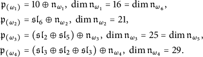 $$ \begin{align*} \mathfrak p_{(\omega_{1})} &= {10}\oplus \mathfrak n_{\omega_{1}}, \ \dim \mathfrak n_{\omega_{1}}=16 = \dim\mathfrak n_{\omega_{6}},\\ \mathfrak p_{(\omega_{2})} &= \mathfrak{sl}_{6}\oplus \mathfrak n_{\omega_{2}}, \ \dim \mathfrak n_{\omega_{2}}=21,\\ \mathfrak p_{(\omega_{3})} &= (\mathfrak{sl}_{2}\oplus\mathfrak{sl}_{5})\oplus \mathfrak n_{\omega_{3}}, \ \dim \mathfrak n_{\omega_{3}}=25 = \dim\mathfrak n_{\omega_{5}},\\ \mathfrak p_{(\omega_{4})} &= (\mathfrak{sl}_{3}\oplus\mathfrak{sl}_{2}\oplus\mathfrak{sl}_{3})\oplus \mathfrak n_{\omega_{4}}, \ \dim \mathfrak n_{\omega_{4}}=29. \end{align*} $$
Since $\dim \mathfrak n_{\omega _{1}+\omega _{2}}=\dim \mathfrak n_{\omega _{2}+\omega _{6}}=\frac {1}{2}(\dim {\mathsf {E}_{6}}-\dim \mathsf {A}_{4}-2)=26$
and
$\dim \mathfrak n_{\omega _{1}+\omega _{2}}=\dim \mathfrak n_{\omega _{2}+\omega _{6}}=\frac {1}{2}(\dim {\mathsf {E}_{6}}-\dim \mathsf {A}_{4}-2)=26$
and $\dim \mathfrak n_{\omega _{1}+\omega _{6}}=\frac {1}{2}(\dim {\mathsf {E}_{6}}-\dim {\mathsf {D}_{4}}-2)=24$
, we have only to consider the cases
$\dim \mathfrak n_{\omega _{1}+\omega _{6}}=\frac {1}{2}(\dim {\mathsf {E}_{6}}-\dim {\mathsf {D}_{4}}-2)=24$
, we have only to consider the cases $\lambda \in \{\omega _{1},\omega _{2}, \omega _{6}\}$
.
$\lambda \in \{\omega _{1},\omega _{2}, \omega _{6}\}$
.
(1) We have $\mathfrak p_{(\omega _{1})} = {10}\oplus \mathfrak n_{\omega _{1}}$
, and
$\mathfrak p_{(\omega _{1})} = {10}\oplus \mathfrak n_{\omega _{1}}$
, and $\mathfrak n_{\omega _{1}}=V(\alpha _1)$
is the irreducible representation
$\mathfrak n_{\omega _{1}}=V(\alpha _1)$
is the irreducible representation $V_{\omega _{4}}$
of
$V_{\omega _{4}}$
of ${10}$
of dimension
${10}$
of dimension $16$
. Since
$16$
. Since $16>r_{{\mathsf {D}_{5}}}=9$
, we see that the codimension of
$16>r_{{\mathsf {D}_{5}}}=9$
, we see that the codimension of $\mathfrak g_x$
in
$\mathfrak g_x$
in $\mathfrak p_{(\omega _1)}$
is at least 9. Thus,
$\mathfrak p_{(\omega _1)}$
is at least 9. Thus, $\dim O =\operatorname {\mathrm {codim}}\mathfrak g_{x} \geq \operatorname {\mathrm {codim}} \mathfrak p_{(\omega _{1})}+9 = 17+9 = 26$
.
$\dim O =\operatorname {\mathrm {codim}}\mathfrak g_{x} \geq \operatorname {\mathrm {codim}} \mathfrak p_{(\omega _{1})}+9 = 17+9 = 26$
.
(2) We have $\mathfrak p_{(\omega _{2})} = \mathfrak {sl}_{6}\oplus \mathfrak n_{\omega _{2}}$
,
$\mathfrak p_{(\omega _{2})} = \mathfrak {sl}_{6}\oplus \mathfrak n_{\omega _{2}}$
, $\mathfrak n_{\omega _2} = V(\alpha _2)\oplus \mathbb {K}$
, and
$\mathfrak n_{\omega _2} = V(\alpha _2)\oplus \mathbb {K}$
, and $V(\alpha _2)$
is the irreducible representation
$V(\alpha _2)$
is the irreducible representation $V_{\omega _3}=\bigwedge ^3\mathbb {K}^{6}$
of
$V_{\omega _3}=\bigwedge ^3\mathbb {K}^{6}$
of $\mathfrak {sl}_{6}$
of dimension
$\mathfrak {sl}_{6}$
of dimension $20$
. Since
$20$
. Since $20>r_{\operatorname {\mathrm {SL}}_{6}}=10$
, we see that the codimension of
$20>r_{\operatorname {\mathrm {SL}}_{6}}=10$
, we see that the codimension of $\mathfrak g_{x}$
in
$\mathfrak g_{x}$
in $\mathfrak p_{(\omega _{2})}$
is at least
$\mathfrak p_{(\omega _{2})}$
is at least $10$
. Thus,
$10$
. Thus, $\dim O =\operatorname {\mathrm {codim}}\mathfrak g_{x} \geq \operatorname {\mathrm {codim}} \mathfrak p_{(\omega _{2})}+10 = 22+10 = 32$
.
$\dim O =\operatorname {\mathrm {codim}}\mathfrak g_{x} \geq \operatorname {\mathrm {codim}} \mathfrak p_{(\omega _{2})}+10 = 22+10 = 32$
.
(3) The case $\mathfrak p_{(\omega _{6})}$
is similar to
$\mathfrak p_{(\omega _{6})}$
is similar to $\mathfrak p_{(\omega _{1})}$
from (1).
$\mathfrak p_{(\omega _{1})}$
from (1).
Remark 5.13 We have just shown that any quasi-affine orbit of dimension ${<}26$
is minimal. Furthermore,
${<}26$
is minimal. Furthermore, $\dim O_{\lambda }=\dim \mathfrak n_{\lambda }+1$
by (5.3) and Section 5.3. From above, we get
$\dim O_{\lambda }=\dim \mathfrak n_{\lambda }+1$
by (5.3) and Section 5.3. From above, we get
 $$\begin{align*}\dim O_{\omega_1}=\dim O_{\omega_6}=17,\quad \dim O_{\omega_2}=22,\quad \dim O_{\omega_1+\omega_6}=25, \end{align*}$$
and all other minimal orbits are of dimension ${\geq}26$
by (5.4). Moreover,
${\geq}26$
by (5.4). Moreover, $r_{{\mathsf {E}_{6}}}=26$
appears as dimension of an affine orbit as well as of the minimal orbits
$r_{{\mathsf {E}_{6}}}=26$
appears as dimension of an affine orbit as well as of the minimal orbits $O_{\omega _3}$
and
$O_{\omega _3}$
and $O_{\omega _5}$
.
$O_{\omega _5}$
.
5.6.4 The type
${\mathsf {E}_{7}}$

Let G be simply connected of type ${\mathsf {E}_{7}}$
and
${\mathsf {E}_{7}}$
and $\mathfrak g = \operatorname {\mathrm {Lie}} G$
, and let O be a nonminimal and nontrivial quasi-affine orbit. We have to show that
$\mathfrak g = \operatorname {\mathrm {Lie}} G$
, and let O be a nonminimal and nontrivial quasi-affine orbit. We have to show that $\dim O \geq 45$
. We have seen above that it suffices to consider those embeddings
$\dim O \geq 45$
. We have seen above that it suffices to consider those embeddings $\mathfrak g_{x}\subset \mathfrak p_{(\lambda )}$
where
$\mathfrak g_{x}\subset \mathfrak p_{(\lambda )}$
where $\dim \mathfrak n_{\lambda } < 43$
.
$\dim \mathfrak n_{\lambda } < 43$
.
If $\lambda $
is a fundamental weight, then we find
$\lambda $
is a fundamental weight, then we find
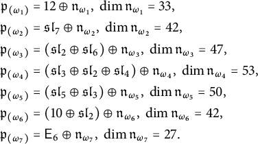 $$ \begin{align*} \mathfrak p_{(\omega_{1})} &= {12}\oplus \mathfrak n_{\omega_{1}}, \ \dim \mathfrak n_{\omega_{1}}=33,\\ \mathfrak p_{(\omega_{2})} &= \mathfrak{sl}_{7}\oplus \mathfrak n_{\omega_{2}}, \ \dim \mathfrak n_{\omega_{2}}=42,\\ \mathfrak p_{(\omega_{3})} &= (\mathfrak{sl}_{2}\oplus\mathfrak{sl}_{6})\oplus \mathfrak n_{\omega_{3}}, \ \dim \mathfrak n_{\omega_{3}}=47,\\ \mathfrak p_{(\omega_{4})} &= (\mathfrak{sl}_{3}\oplus\mathfrak{sl}_{2}\oplus\mathfrak{sl}_{4})\oplus \mathfrak n_{\omega_{4}}, \ \dim \mathfrak n_{\omega_{4}}=53,\\ \mathfrak p_{(\omega_{5})} &= (\mathfrak{sl}_{5}\oplus\mathfrak{sl}_{3})\oplus \mathfrak n_{\omega_{5}}, \ \dim \mathfrak n_{\omega_{5}}=50,\\ \mathfrak p_{(\omega_{6})} &= ({10}\oplus\mathfrak{sl}_{2})\oplus \mathfrak n_{\omega_{6}}, \ \dim \mathfrak n_{\omega_{6}}=42,\\ \mathfrak p_{(\omega_{7})} &= {\mathsf{E}_{6}}\oplus \mathfrak n_{\omega_{7}}, \ \dim \mathfrak n_{\omega_{7}}=27. \end{align*} $$
Since $\dim \mathfrak n_{\omega _{1}+\omega _{2}}=\frac {1}{2}(\dim {\mathsf {E}_{7}}-\dim \mathsf {A}_{5}-2)=48$
,
$\dim \mathfrak n_{\omega _{1}+\omega _{2}}=\frac {1}{2}(\dim {\mathsf {E}_{7}}-\dim \mathsf {A}_{5}-2)=48$
, $\dim \mathfrak n_{\omega _{1}+\omega _{6}}=\frac {1}{2}(\dim {\mathsf {E}_{7}}-\dim {\mathsf {D}_{4}} -\dim {\mathsf {A}_{1}}-2)=50$
,
$\dim \mathfrak n_{\omega _{1}+\omega _{6}}=\frac {1}{2}(\dim {\mathsf {E}_{7}}-\dim {\mathsf {D}_{4}} -\dim {\mathsf {A}_{1}}-2)=50$
, $\dim \mathfrak n_{\omega _{1}+\omega _{7}} = \frac {1}{2}(\dim {\mathsf {E}_{7}}-\dim {\mathsf {D}_{5}}-2)=43$
,
$\dim \mathfrak n_{\omega _{1}+\omega _{7}} = \frac {1}{2}(\dim {\mathsf {E}_{7}}-\dim {\mathsf {D}_{5}}-2)=43$
, $\dim \mathfrak n_{\omega _{2}+\omega _{6}} = \frac {1}{2}(\dim {\mathsf {E}_{7}}-\dim \mathsf {A}_{4}-\dim {\mathsf {A}_{1}}-2)=52$
,
$\dim \mathfrak n_{\omega _{2}+\omega _{6}} = \frac {1}{2}(\dim {\mathsf {E}_{7}}-\dim \mathsf {A}_{4}-\dim {\mathsf {A}_{1}}-2)=52$
, $\dim \mathfrak n_{\omega _{2}+\omega _{7}} = \frac {1}{2}(\dim {\mathsf {E}_{7}}-\dim \mathsf {A}_{5}-2)=48$
, and
$\dim \mathfrak n_{\omega _{2}+\omega _{7}} = \frac {1}{2}(\dim {\mathsf {E}_{7}}-\dim \mathsf {A}_{5}-2)=48$
, and $\dim \mathfrak n_{\omega _{6}+\omega _{7}} = \frac {1}{2}(\dim {\mathsf {E}_{7}}-\dim {\mathsf {D}_{5}}-2)=43$
, we have only to consider the cases
$\dim \mathfrak n_{\omega _{6}+\omega _{7}} = \frac {1}{2}(\dim {\mathsf {E}_{7}}-\dim {\mathsf {D}_{5}}-2)=43$
, we have only to consider the cases $\lambda \in \{\omega _{1},\omega _{2}, \omega _{6},\omega _{7}\}$
.
$\lambda \in \{\omega _{1},\omega _{2}, \omega _{6},\omega _{7}\}$
.
(1) We have $\mathfrak p_{(\omega _{1})} = {12}\oplus \mathfrak n_{\omega _{1}}$
,
$\mathfrak p_{(\omega _{1})} = {12}\oplus \mathfrak n_{\omega _{1}}$
, $\mathfrak n_{\omega _1} = V(\alpha _1)\oplus \mathbb {K}$
, and
$\mathfrak n_{\omega _1} = V(\alpha _1)\oplus \mathbb {K}$
, and $V(\alpha _{1})$
is the irreducible representation
$V(\alpha _{1})$
is the irreducible representation $V_{\omega _{5}}$
of
$V_{\omega _{5}}$
of ${12}$
of dimension
${12}$
of dimension $32>r_{{\mathsf {D}_{6}}}=11$
. Thus, the codimension of
$32>r_{{\mathsf {D}_{6}}}=11$
. Thus, the codimension of $\mathfrak g_{x}$
in
$\mathfrak g_{x}$
in $\mathfrak p_{(\omega _{1})}$
is at least
$\mathfrak p_{(\omega _{1})}$
is at least $11$
, and so
$11$
, and so $\dim O =\operatorname {\mathrm {codim}}\mathfrak g_{x} \geq \operatorname {\mathrm {codim}} \mathfrak p_{(\omega _{1})}+11 = 34+11 = 45$
. Moreover, the subalgebra
$\dim O =\operatorname {\mathrm {codim}}\mathfrak g_{x} \geq \operatorname {\mathrm {codim}} \mathfrak p_{(\omega _{1})}+11 = 34+11 = 45$
. Moreover, the subalgebra $\mathfrak h:={11}\oplus \mathfrak n_{\omega _1}\subset \mathfrak g$
is the Lie algebra of a subgroup H of codimension
$\mathfrak h:={11}\oplus \mathfrak n_{\omega _1}\subset \mathfrak g$
is the Lie algebra of a subgroup H of codimension $34+11=45$
which has no characters. By Remark 5.10, we see that
$34+11=45$
which has no characters. By Remark 5.10, we see that $G/H$
is a quasi-affine orbit of dimension 45, and so
$G/H$
is a quasi-affine orbit of dimension 45, and so $d_{\mathsf {E}_{7}} \leq 45$
.
$d_{\mathsf {E}_{7}} \leq 45$
.
(2) We have $\mathfrak p_{(\omega _{2})} = \mathfrak {sl}_{7}\oplus \mathfrak n_{\omega _{2}}$
,
$\mathfrak p_{(\omega _{2})} = \mathfrak {sl}_{7}\oplus \mathfrak n_{\omega _{2}}$
, $\mathfrak n_{\omega _2} = V(\alpha _2)\oplus \mathbb {K}^7$
, and
$\mathfrak n_{\omega _2} = V(\alpha _2)\oplus \mathbb {K}^7$
, and $V(\alpha _{2})$
is the irreducible representation
$V(\alpha _{2})$
is the irreducible representation $V_{\omega _4}=\bigwedge ^{4}\mathbb {K}^{7}$
of
$V_{\omega _4}=\bigwedge ^{4}\mathbb {K}^{7}$
of $\mathfrak {sl}_{7}$
of dimension
$\mathfrak {sl}_{7}$
of dimension $35>r_{\operatorname {\mathrm {SL}}_{7}}=12$
. Thus, the codimension of
$35>r_{\operatorname {\mathrm {SL}}_{7}}=12$
. Thus, the codimension of $\mathfrak g_{x}$
in
$\mathfrak g_{x}$
in $\mathfrak p_{(\omega _{2})}$
is at least
$\mathfrak p_{(\omega _{2})}$
is at least $12$
, and so
$12$
, and so $\dim O =\operatorname {\mathrm {codim}}\mathfrak g_{x} \geq \operatorname {\mathrm {codim}} \mathfrak p_{(\omega _{2})}+12 = 43+12 = 55>45$
.
$\dim O =\operatorname {\mathrm {codim}}\mathfrak g_{x} \geq \operatorname {\mathrm {codim}} \mathfrak p_{(\omega _{2})}+12 = 43+12 = 55>45$
.
(3) We have $\mathfrak p_{(\omega _{6})} = ({10}\oplus \mathfrak {sl}_{2})\oplus \mathfrak n_{\omega _{6}}$
,
$\mathfrak p_{(\omega _{6})} = ({10}\oplus \mathfrak {sl}_{2})\oplus \mathfrak n_{\omega _{6}}$
, $\mathfrak n_{\omega _6} = V(\alpha _6)\oplus \mathbb {K}^{10}$
, and
$\mathfrak n_{\omega _6} = V(\alpha _6)\oplus \mathbb {K}^{10}$
, and $V(\alpha _{6})$
is the irreducible representation
$V(\alpha _{6})$
is the irreducible representation $V_{\omega _{5}}\otimes \mathbb {K}^{2}$
of
$V_{\omega _{5}}\otimes \mathbb {K}^{2}$
of ${10}\oplus \mathfrak {sl}_{2}$
of dimension
${10}\oplus \mathfrak {sl}_{2}$
of dimension $2\times 16=32>r_{{\mathsf {D}_{5}}\times {\mathsf {A}_{1}}}=2$
. Thus, the codimension of
$2\times 16=32>r_{{\mathsf {D}_{5}}\times {\mathsf {A}_{1}}}=2$
. Thus, the codimension of $\mathfrak g_{x}$
in
$\mathfrak g_{x}$
in $\mathfrak p_{(\omega _{6})}$
is at least
$\mathfrak p_{(\omega _{6})}$
is at least $2$
, and so
$2$
, and so $\dim O =\operatorname {\mathrm {codim}}\mathfrak g_{x} \geq \operatorname {\mathrm {codim}} \mathfrak p_{(\omega _{6})}+2 = 43+2 = 45$
.
$\dim O =\operatorname {\mathrm {codim}}\mathfrak g_{x} \geq \operatorname {\mathrm {codim}} \mathfrak p_{(\omega _{6})}+2 = 43+2 = 45$
.
(4) We have $\mathfrak p_{(\omega _{7})}={\mathsf {E}_{6}} \oplus \mathfrak n_{\omega _{7}}$
, and
$\mathfrak p_{(\omega _{7})}={\mathsf {E}_{6}} \oplus \mathfrak n_{\omega _{7}}$
, and $V(\alpha _{7}) = \mathfrak n_{\omega _{7}}$
is the irreducible representation
$V(\alpha _{7}) = \mathfrak n_{\omega _{7}}$
is the irreducible representation $V_{\omega _{6}}$
of
$V_{\omega _{6}}$
of ${\mathsf {E}_{6}}$
of dimension
${\mathsf {E}_{6}}$
of dimension $27>r_{{\mathsf {E}_{6}}}=26$
. Thus, the codimension of
$27>r_{{\mathsf {E}_{6}}}=26$
. Thus, the codimension of $\mathfrak g_{x}$
in
$\mathfrak g_{x}$
in $\mathfrak p_{(\omega _{7})}$
is at least
$\mathfrak p_{(\omega _{7})}$
is at least $26$
, and so
$26$
, and so $\dim O =\operatorname {\mathrm {codim}}\mathfrak g_{x} \geq \operatorname {\mathrm {codim}} \mathfrak p_{(\omega _{7})}+26 = 28+26 = 54>45$
.
$\dim O =\operatorname {\mathrm {codim}}\mathfrak g_{x} \geq \operatorname {\mathrm {codim}} \mathfrak p_{(\omega _{7})}+26 = 28+26 = 54>45$
.
5.6.5 The type
${\mathsf {E}_{8}}$

Let G be simply connected of type ${\mathsf {E}_{8}}$
and
${\mathsf {E}_{8}}$
and $\mathfrak g = \operatorname {\mathrm {Lie}} G$
, and let O be a nonminimal and nontrivial quasi-affine orbit. We have to show that
$\mathfrak g = \operatorname {\mathrm {Lie}} G$
, and let O be a nonminimal and nontrivial quasi-affine orbit. We have to show that $\dim O \geq 86$
. We have seen above that it suffices to consider those embeddings
$\dim O \geq 86$
. We have seen above that it suffices to consider those embeddings $\mathfrak g_{x}\subset \mathfrak p_{(\lambda )}$
where
$\mathfrak g_{x}\subset \mathfrak p_{(\lambda )}$
where $\dim \mathfrak n_{\lambda } < 84$
.
$\dim \mathfrak n_{\lambda } < 84$
.
If $\lambda $
is a fundamental weight, then we find
$\lambda $
is a fundamental weight, then we find
 $$ \begin{align*} \mathfrak p_{(\omega_{1})} &= {14}\oplus \mathfrak n_{\omega_{1}}, \ \dim \mathfrak n_{\omega_{1}}=78,\\ \mathfrak p_{(\omega_{2})} &= \mathfrak{sl}_{8}\oplus \mathfrak n_{\omega_{2}}, \ \dim \mathfrak n_{\omega_{2}}=92,\\ \mathfrak p_{(\omega_{3})} &= (\mathfrak{sl}_{2}\oplus\mathfrak{sl}_{7})\oplus \mathfrak n_{\omega_{3}}, \ \dim \mathfrak n_{\omega_{3}}=98,\\ \mathfrak p_{(\omega_{4})} &= (\mathfrak{sl}_{3}\oplus\mathfrak{sl}_{2}\oplus\mathfrak{sl}_{5})\oplus \mathfrak n_{\omega_{4}}, \ \dim \mathfrak n_{\omega_{4}}=106,\\ \mathfrak p_{(\omega_{5})} &= (\mathfrak{sl}_{5}\oplus\mathfrak{sl}_{4})\oplus \mathfrak n_{\omega_{5}}, \ \dim \mathfrak n_{\omega_{5}}=104,\\ \mathfrak p_{(\omega_{6})} &= ({10}\oplus\mathfrak{sl}_{3})\oplus \mathfrak n_{\omega_{6}}, \ \dim \mathfrak n_{\omega_{6}}=97,\\ \mathfrak p_{(\omega_{7})} &= ({\mathsf{E}_{6}}\oplus \mathfrak{sl}_{2}) \oplus \mathfrak n_{\omega_{7}}, \ \dim \mathfrak n_{\omega_{7}}=83,\\ \mathfrak p_{(\omega_{8})} &= {\mathsf{E}_{7}} \oplus \mathfrak n_{\omega_{8}}, \ \dim \mathfrak n_{\omega_{8}}=57. \end{align*} $$
Since $\dim \mathfrak n_{\omega _{1}+\omega _{7}}=\frac {1}{2}(\dim {\mathsf {E}_{8}}-\dim {\mathsf {D}_{5}}-\dim {\mathsf {A}_{1}}-2)=99$
,
$\dim \mathfrak n_{\omega _{1}+\omega _{7}}=\frac {1}{2}(\dim {\mathsf {E}_{8}}-\dim {\mathsf {D}_{5}}-\dim {\mathsf {A}_{1}}-2)=99$
, $\dim \mathfrak n_{\omega _{1}+\omega _{8}}=\frac {1}{2}(\dim {\mathsf {E}_{8}}-\dim {\mathsf {D}_{6}} -2)=90$
, and
$\dim \mathfrak n_{\omega _{1}+\omega _{8}}=\frac {1}{2}(\dim {\mathsf {E}_{8}}-\dim {\mathsf {D}_{6}} -2)=90$
, and $\dim \mathfrak n_{\omega _{7}+\omega _{8}} = \frac {1}{2}(\dim {\mathsf {E}_{8}}-\dim {\mathsf {E}_{6}}-2)=84$
, we have only to consider the cases
$\dim \mathfrak n_{\omega _{7}+\omega _{8}} = \frac {1}{2}(\dim {\mathsf {E}_{8}}-\dim {\mathsf {E}_{6}}-2)=84$
, we have only to consider the cases $\lambda \in \{\omega _{1},\omega _{7}, \omega _{8}\}$
.
$\lambda \in \{\omega _{1},\omega _{7}, \omega _{8}\}$
.
(1) We have $\mathfrak p_{(\omega _{1})} = {14}\oplus \mathfrak n_{\omega _{1}}$
,
$\mathfrak p_{(\omega _{1})} = {14}\oplus \mathfrak n_{\omega _{1}}$
, $\mathfrak n_{\omega _1} = V(\alpha _1)\oplus \mathbb {K}^{14}$
, and
$\mathfrak n_{\omega _1} = V(\alpha _1)\oplus \mathbb {K}^{14}$
, and $V(\alpha _{1})$
is the irreducible representation
$V(\alpha _{1})$
is the irreducible representation $V_{\omega _{7}}$
of
$V_{\omega _{7}}$
of ${14}$
of dimension
${14}$
of dimension $64>r_{{\mathsf {D}_{7}}}=13$
. Thus, the codimension of
$64>r_{{\mathsf {D}_{7}}}=13$
. Thus, the codimension of $\mathfrak g_{x}$
in
$\mathfrak g_{x}$
in $\mathfrak p_{(\omega _{1})}$
is at least
$\mathfrak p_{(\omega _{1})}$
is at least $13$
, and so
$13$
, and so $\dim O =\operatorname {\mathrm {codim}}\mathfrak g_{x} \geq \operatorname {\mathrm {codim}} \mathfrak p_{(\omega _{1})}+13 = 79+13 = 92>86$
.
$\dim O =\operatorname {\mathrm {codim}}\mathfrak g_{x} \geq \operatorname {\mathrm {codim}} \mathfrak p_{(\omega _{1})}+13 = 79+13 = 92>86$
.
(2) We have $\mathfrak p_{(\omega _{7})} = ({\mathsf {E}_{6}}\oplus \mathfrak {sl}_{2})\oplus \mathfrak n_{\omega _{7}}$
, and
$\mathfrak p_{(\omega _{7})} = ({\mathsf {E}_{6}}\oplus \mathfrak {sl}_{2})\oplus \mathfrak n_{\omega _{7}}$
, and $V(\alpha _{7})\subset \mathfrak n_{\omega _{7}}$
is the irreducible representation
$V(\alpha _{7})\subset \mathfrak n_{\omega _{7}}$
is the irreducible representation $V_{\omega _{6}}\otimes \mathbb {K}^{2}$
of
$V_{\omega _{6}}\otimes \mathbb {K}^{2}$
of ${\mathsf {E}_{6}}\oplus \mathfrak {sl}_{2}$
of dimension
${\mathsf {E}_{6}}\oplus \mathfrak {sl}_{2}$
of dimension $2\times 27=54>r_{{\mathsf {E}_{6}}\times {\mathsf {A}_{1}}}=2$
. Thus, the codimension of
$2\times 27=54>r_{{\mathsf {E}_{6}}\times {\mathsf {A}_{1}}}=2$
. Thus, the codimension of $\mathfrak g_{x}$
in
$\mathfrak g_{x}$
in $\mathfrak p_{(\omega _{7})}$
is at least
$\mathfrak p_{(\omega _{7})}$
is at least $2$
, and so
$2$
, and so $\dim O =\operatorname {\mathrm {codim}}\mathfrak g_{x} \geq \operatorname {\mathrm {codim}} \mathfrak p_{(\omega _{7})}+2 = 84+2 = 86$
.
$\dim O =\operatorname {\mathrm {codim}}\mathfrak g_{x} \geq \operatorname {\mathrm {codim}} \mathfrak p_{(\omega _{7})}+2 = 84+2 = 86$
.
(3) We have $\mathfrak p_{(\omega _{8})}={\mathsf {E}_{7}} \oplus \mathfrak n_{\omega _{8}}$
,
$\mathfrak p_{(\omega _{8})}={\mathsf {E}_{7}} \oplus \mathfrak n_{\omega _{8}}$
, $\mathfrak n_{\omega _8} = V(\alpha _8) \oplus \mathbb {K}$
, and
$\mathfrak n_{\omega _8} = V(\alpha _8) \oplus \mathbb {K}$
, and $V(\alpha _{8})$
is the irreducible representation
$V(\alpha _{8})$
is the irreducible representation $V_{\omega _{7}}$
of
$V_{\omega _{7}}$
of ${\mathsf {E}_{7}}$
of dimension
${\mathsf {E}_{7}}$
of dimension $56>r_{{\mathsf {E}_{7}}}=54$
. Thus, the codimension of
$56>r_{{\mathsf {E}_{7}}}=54$
. Thus, the codimension of $\mathfrak g_{x}$
in
$\mathfrak g_{x}$
in $\mathfrak p_{(\omega _{8})}$
is at least
$\mathfrak p_{(\omega _{8})}$
is at least $54$
, and so
$54$
, and so $\dim O =\operatorname {\mathrm {codim}}\mathfrak g_{x} \geq \operatorname {\mathrm {codim}} \mathfrak p_{(\omega _{8})}+54 = 58+54 = 112> 86$
.
$\dim O =\operatorname {\mathrm {codim}}\mathfrak g_{x} \geq \operatorname {\mathrm {codim}} \mathfrak p_{(\omega _{8})}+54 = 58+54 = 112> 86$
.
(4) The subalgebra $\mathfrak p_{(\omega _7+\omega _8)} = {\mathsf {E}_{6}}\oplus \mathfrak n_{\omega _7+\omega _8}$
corresponds to a closed subgroup
$\mathfrak p_{(\omega _7+\omega _8)} = {\mathsf {E}_{6}}\oplus \mathfrak n_{\omega _7+\omega _8}$
corresponds to a closed subgroup $H\subset G$
of codimension
$H\subset G$
of codimension $84+2=86$
which has no characters. Thus, by Remark 5.10,
$84+2=86$
which has no characters. Thus, by Remark 5.10, $G/H$
is a quasi-affine orbit of dimension 86, and so
$G/H$
is a quasi-affine orbit of dimension 86, and so $d_{\mathsf {E}_{8}} \leq 86$
.
$d_{\mathsf {E}_{8}} \leq 86$
.
For these computations, we used the Computer Algebra Program LiE [Reference van Leeuwen, Cohen and Lisser23] (cf. the version of our paper on the arXiv [Reference Kraft, Regeta and Zimmermann21, Section 5.7]). It can also be done directly using the following facts (see Remark 5.1).
-
• The Dynkin diagram of
$\mathfrak d_i:=[\mathfrak l_{\omega _i},\mathfrak l_{\omega _i}]$
is obtained by removing the ith node from the Dynkin diagram of G. -
• The Cartan numbers
$\langle \alpha _i,\alpha _j\rangle $
are the coefficients of the decomposition of the lowest weight
$\alpha _i|_{\mathfrak d_i}$
of
$V(\alpha _i)$
with respect to the fundamental weights of
$\mathfrak d_i$
. -
• Using the highest root
$\alpha _{\text {max}}$
of
$\mathfrak g$
visible from the extended Dynkin diagram, we see that
$\omega _{\text {max}} |_{\mathfrak d_i}$
is the highest weight of a simple
$\mathfrak d_i$
-submodule of
$\mathfrak n_{\omega _i}$
which coincides with
$V(\alpha _i)$
only if
$\mathfrak n_{\omega _i} = V(\alpha _i)$
.


Here is an example suggested by the referee.
Example 5.14 In Section 5.6.5(2), one sees from the Dynkin diagram that $\mathfrak d_{7} = {\mathsf {E}_{6}} \oplus \mathfrak {sl}_2$
, and the nonzero Cartan numbers are
$\mathfrak d_{7} = {\mathsf {E}_{6}} \oplus \mathfrak {sl}_2$
, and the nonzero Cartan numbers are $\langle \alpha _7,\alpha _6\rangle = \langle \alpha _7, \alpha _8\rangle = -1$
. By duality, the highest weight of
$\langle \alpha _7,\alpha _6\rangle = \langle \alpha _7, \alpha _8\rangle = -1$
. By duality, the highest weight of $V(\alpha _7)$
is the sum of two fundamental weights corresponding to the simple roots
$V(\alpha _7)$
is the sum of two fundamental weights corresponding to the simple roots $\alpha _1$
of
$\alpha _1$
of ${\mathsf {E}_{6}}$
and
${\mathsf {E}_{6}}$
and $\alpha _8$
of
$\alpha _8$
of $\mathfrak {sl}_2$
. Hence,
$\mathfrak {sl}_2$
. Hence, $V(\alpha _7)$
is the tensor product of the minimal representation of
$V(\alpha _7)$
is the tensor product of the minimal representation of ${\mathsf {E}_{6}}$
with
${\mathsf {E}_{6}}$
with $\mathbb {K}^2$
, and is of dimension
$\mathbb {K}^2$
, and is of dimension $27\times 2=54$
.
$27\times 2=54$
.
Moreover, the only nonzero Cartan number of $\alpha _{\text {max}}$
is
$\alpha _{\text {max}}$
is $\langle \alpha _{\text {max}},\alpha _8\rangle = 1$
. Hence, the respective representation of
$\langle \alpha _{\text {max}},\alpha _8\rangle = 1$
. Hence, the respective representation of $\mathfrak d_7$
is
$\mathfrak d_7$
is $\mathbb {K}^2$
. Finally, since
$\mathbb {K}^2$
. Finally, since $\langle \alpha _{\text {max}},\alpha _8\rangle> 0$
,
$\langle \alpha _{\text {max}},\alpha _8\rangle> 0$
, $\alpha := \alpha _{\text {max}}-\alpha _8$
is a root, and
$\alpha := \alpha _{\text {max}}-\alpha _8$
is a root, and $\beta := \alpha - \alpha _7$
is a root for the same reason. As
$\beta := \alpha - \alpha _7$
is a root for the same reason. As $\beta + \alpha _j$
is not a root, except for
$\beta + \alpha _j$
is not a root, except for $j=7$
,
$j=7$
, $\beta |_{\mathfrak d_7}$
is the highest weight of another simple
$\beta |_{\mathfrak d_7}$
is the highest weight of another simple $\mathfrak d_7$
-submodule of
$\mathfrak d_7$
-submodule of $\mathfrak n_{\omega _7}$
, with the only nonzero Cartan number
$\mathfrak n_{\omega _7}$
, with the only nonzero Cartan number $\langle \beta , \alpha _6\rangle = 1$
. Hence, this submodule is given by the other minimal representation of
$\langle \beta , \alpha _6\rangle = 1$
. Hence, this submodule is given by the other minimal representation of ${\mathsf {E}_{6}}$
. By dimension count, we have found all simple summands of
${\mathsf {E}_{6}}$
. By dimension count, we have found all simple summands of $\mathfrak n_{\omega _7}$
.
$\mathfrak n_{\omega _7}$
.
Acknowledgment
We would like to thank Oksana Yakimova for her help with the computation of the invariant $d_G$
and Michel Brion for interesting and helpful discussions. We would also like to thank the referees for their very careful reading of the manuscript, pointing out many typos and inaccuracies.
$d_G$
and Michel Brion for interesting and helpful discussions. We would also like to thank the referees for their very careful reading of the manuscript, pointing out many typos and inaccuracies.


 Open access