


1. Introduction
Inspired by the pioneering work [Reference Erdős and Rényi16] of Erdős and Rényi in 1960, random discrete structures have been systematically studied in literally thousands of contributions. One of the initial motivations of this research was to study open problems in graph theory and combinatorics. In the following decades, however, the application of such models proved useful as a unified approach to treat a variety of problems in several fields. To mention just a few, random graphs turned out to be valuable in solving fundamental theoretical and practical problems, such as the development of error correcting codes [Reference Kudekar, Richardson and Urbanke29], the study of statistical inference through the stochastic block model [Reference Abbe1], and the establishment of lower bounds in complexity theory [Reference Feige18, Reference Galanis, Štefankovič and Vigoda21].
The results of the past years of research suggest the existence of phase transitions in many classes of random discrete structures, i.e. a specific value of a given model parameter at which the properties of the system in question change dramatically. Random constraint satisfaction problems are one specific type of such structures that tend to exhibit this remarkable property and that are of particular interest in too many areas to mention, covering complexity theory, combinatorics, statistical mechanics, artificial intelligence, biology, engineering and economics. An instance of a CSP is defined by a set of variables that take values in – typically finite – domains and a set of constraints, where each constraint is satisfied for specific assignments of the subset of variables it involves. A major computational challenge is to determine whether such an instance is satisfiable, i.e. to determine if there is an assignment of all variables that satisfies all constraints. Since the 1980s non-rigorous methods have been introduced in statistical physics that are targeted at the analysis of phase transitions in random CSPs [Reference Krzakala, Ricci-Tersenghi, Zdeborová, Zecchina, Tramel and Cugliandolo28, Reference Mézard and Montanari31, Reference Mézard, Parisi and Virasoro32]. Within this line of research, a variety of exciting and unexpected phenomena were discovered, for example the existence of multiple phase transitions with respect to the structure of the solution space; these transitions may have a significant impact on the hardness of the underlying instances. Since then these methods and the description of the conjectured regimes have been heavily supported by several findings, including the astounding empirical success of randomized algorithms like belief and survey propagation [Reference Braunstein, Mézard and Zecchina5], as well as rigorous verifications, most prominently the phase transition in $k$
-SAT [Reference Ding, Sly and Sun13] (for large
$k$
-SAT [Reference Ding, Sly and Sun13] (for large $k$
) and the condensation phase transition in many important models [Reference Coja-Oghlan, Krzakala, Perkins and Zdeborova9]. However, a complete rigorous study is still a big challenge for computer science and mathematics.
$k$
) and the condensation phase transition in many important models [Reference Coja-Oghlan, Krzakala, Perkins and Zdeborova9]. However, a complete rigorous study is still a big challenge for computer science and mathematics.
Usually, the relevant model parameter of a random CSP is a certain problem specific density as illustrated below. The main focus of research is to study the occurrence of phase transitions in the solution space structure and in particular the existence of (sharp) satisfiability thresholds, i.e. critical values of the density such that the probability that a random CSP admits a solution tends to one as the number of variables tends to infinity for densities below the threshold, while this limiting probability tends to zero for densities above the threshold.
1.1 Random CSPs
Two important types of random CSPs are Erdős-Rényi (ER) type and random regular CSPs. In both cases the number $n$
of variables and the number
$n$
of variables and the number $k$
of variables involved in each constraint is fixed. In ER type CSPs we further fix the number
$k$
of variables involved in each constraint is fixed. In ER type CSPs we further fix the number $m$
of constraints and thereby the density
$m$
of constraints and thereby the density $\alpha ={m}/{n}$
, i.e. the average number of constraints that a variable is involved in. In the regular case we only consider instances where each variable is involved in the same number
$\alpha ={m}/{n}$
, i.e. the average number of constraints that a variable is involved in. In the regular case we only consider instances where each variable is involved in the same number $d$
of constraints, which fixes the density
$d$
of constraints, which fixes the density $d$
as well as the number
$d$
as well as the number $m={dn}/{k}$
of constraints. In a second step we randomly choose the sets of satisfying assignments for each constraint depending on the problem. For example, in the prominent
$m={dn}/{k}$
of constraints. In a second step we randomly choose the sets of satisfying assignments for each constraint depending on the problem. For example, in the prominent $k$
-SAT problem one forbidden assignment is chosen uniformly at random from all possible assignments of the involved binary variables for each constraint independently. Another example is the colouring of hypergraphs, where the constraints are attached to the hyperedges and the variables to the vertices, i.e. the variables involved in a constraint correspond to the vertices incident to a hyperedge. In this case a constraint is violated iff all involved vertices take the same colour.
$k$
-SAT problem one forbidden assignment is chosen uniformly at random from all possible assignments of the involved binary variables for each constraint independently. Another example is the colouring of hypergraphs, where the constraints are attached to the hyperedges and the variables to the vertices, i.e. the variables involved in a constraint correspond to the vertices incident to a hyperedge. In this case a constraint is violated iff all involved vertices take the same colour.
In our work we focus on a class of random regular CSPs in which the choice of satisfying assignments per constraint is fixed in advance, i.e. a class that contains the aforementioned colouring of ( $d$
-regular
$d$
-regular $k$
-uniform) hypergraphs and occupation problems amongst others, but that does not include problems with further randomness in the constraints, like
$k$
-uniform) hypergraphs and occupation problems amongst others, but that does not include problems with further randomness in the constraints, like $k$
-SAT and
$k$
-SAT and $k$
-XORSAT. The lack of randomness on the level of constraints makes this class particularly accessible for an analysis of the asymptotic solution space structure and significantly simplifies simulations based on the well-known population dynamics. Using such simulations, non-rigorous results for this class have been mostly established for the case where the variables are binary valued, so-called occupation problems, or restricted to variants of hypergraph colouring for non-binary variables. Besides the extensive studies on the colouring of simple graphs, i.e.
$k$
-XORSAT. The lack of randomness on the level of constraints makes this class particularly accessible for an analysis of the asymptotic solution space structure and significantly simplifies simulations based on the well-known population dynamics. Using such simulations, non-rigorous results for this class have been mostly established for the case where the variables are binary valued, so-called occupation problems, or restricted to variants of hypergraph colouring for non-binary variables. Besides the extensive studies on the colouring of simple graphs, i.e. $k=2$
, the only rigorous results derived so far consider the arguably most simple type of occupation problems where each constraint is satisfied if exactly one involved variable evaluates to true, which we refer to as
$k=2$
, the only rigorous results derived so far consider the arguably most simple type of occupation problems where each constraint is satisfied if exactly one involved variable evaluates to true, which we refer to as $d$
-regular
$d$
-regular $1$
-in-
$1$
-in- $k$
occupation problem. In our current work we strive to extend these results to general
$k$
occupation problem. In our current work we strive to extend these results to general $d$
-regular
$d$
-regular $r$
-in-
$r$
-in- $k$
occupation problems, i.e. problems where each constraint is satisfied if
$k$
occupation problems, i.e. problems where each constraint is satisfied if $r$
out of the
$r$
out of the $k$
involved variables evaluate to true.
$k$
involved variables evaluate to true.
1.2 Occupation problems
We continue with the formal definition of the class of problems we consider. Let $k$
,
$k$
, $d\in \mathbb {Z}_{\ge 2}$
and
$d\in \mathbb {Z}_{\ge 2}$
and $r\in [k-1] := \{1, \ldots, k-1\}$
be fixed. Additionally, we are given non-empty sets
$r\in [k-1] := \{1, \ldots, k-1\}$
be fixed. Additionally, we are given non-empty sets $V$
of variables and constraints
$V$
of variables and constraints $F$
. We will use the convention to index elements of
$F$
. We will use the convention to index elements of $V$
with the letter
$V$
with the letter $i$
and elements of
$i$
and elements of $F$
with the letter
$F$
with the letter $a$
(and subsequent letters) in the remainder. Then an instance
$a$
(and subsequent letters) in the remainder. Then an instance $o$
of the
$o$
of the $d$
-regular
$d$
-regular $r$
-in-
$r$
-in- $k$
occupation problem is specified by a sequence
$k$
occupation problem is specified by a sequence $o=(v(a))_{a\in F}$
of
$o=(v(a))_{a\in F}$
of $m=|F|$
subsets
$m=|F|$
subsets $v(a)\subseteq V$
of size
$v(a)\subseteq V$
of size $k$
such that each of the
$k$
such that each of the $n=|V|$
variables is contained in
$n=|V|$
variables is contained in $d$
of the subsets. In graph theory the instance
$d$
of the subsets. In graph theory the instance $o$
has a natural interpretation as a
$o$
has a natural interpretation as a $(d,k)$
-biregular graph (or
$(d,k)$
-biregular graph (or $d$
-regular
$d$
-regular $k$
-factor graph) with disjoint node sets
$k$
-factor graph) with disjoint node sets $V \,\dot \cup \, F$
and edges
$V \,\dot \cup \, F$
and edges $\{i,a\}$
if
$\{i,a\}$
if $i\in v(a)$
. By the handshaking lemma, such objects only exist if
$i\in v(a)$
. By the handshaking lemma, such objects only exist if $dn=km$
, which we assume in the following.
$dn=km$
, which we assume in the following.
Given an instance $o$
as just described, an assignment
$o$
as just described, an assignment $x\in \{0,1\}^V$
satisfies a constraint
$x\in \{0,1\}^V$
satisfies a constraint $a\in F$
if
$a\in F$
if $\sum _{i\in v(a)}x_i=r$
, otherwise
$\sum _{i\in v(a)}x_i=r$
, otherwise $x$
violates
$x$
violates $a$
. If
$a$
. If $x$
satisfies all constraints
$x$
satisfies all constraints $a\in F$
, then
$a\in F$
, then $x$
is a solution of
$x$
is a solution of $o$
. Notice that
$o$
. Notice that $d$
times the number of
$d$
times the number of $1$
’s in
$1$
’s in $x$
matches the total number
$x$
matches the total number $rm=rdn/k$
of
$rm=rdn/k$
of $1$
’s observed on the factor side, so
$1$
’s observed on the factor side, so $k$
has to divide
$k$
has to divide $rn$
, which we also assume in the following. We write
$rn$
, which we also assume in the following. We write $z(o)$
for the number of solutions of
$z(o)$
for the number of solutions of $o$
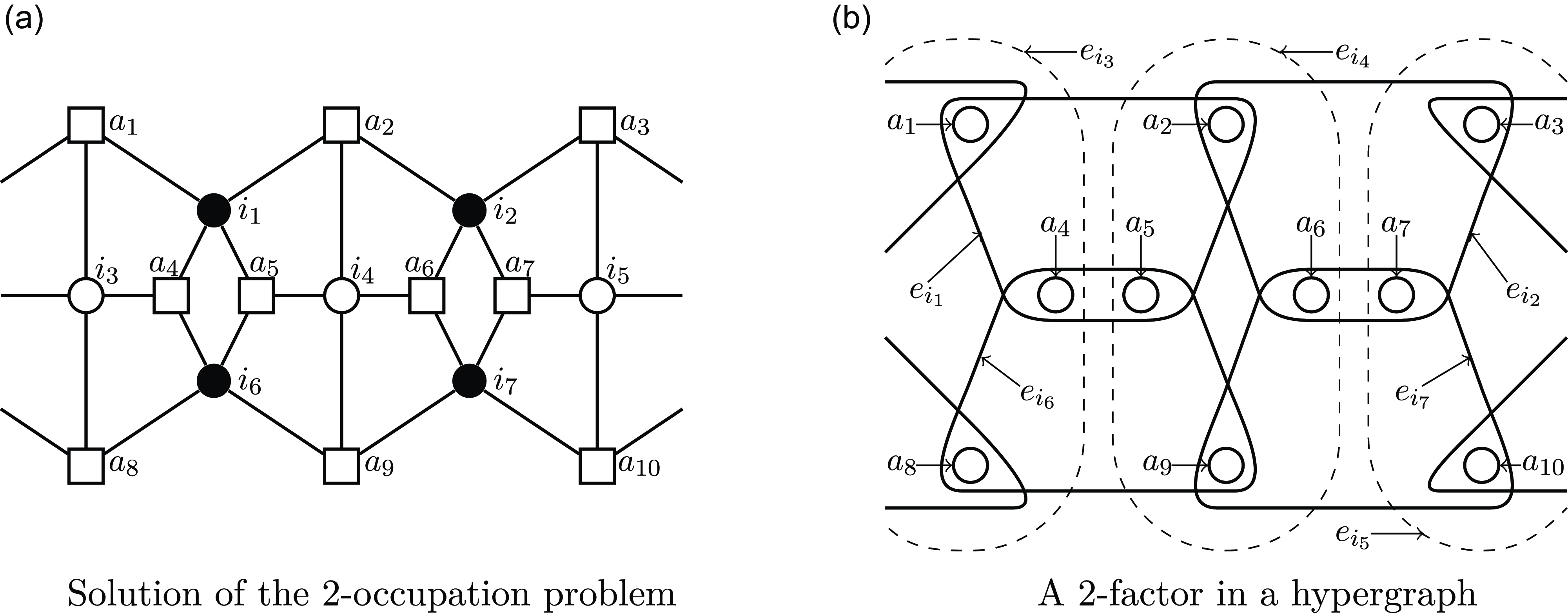
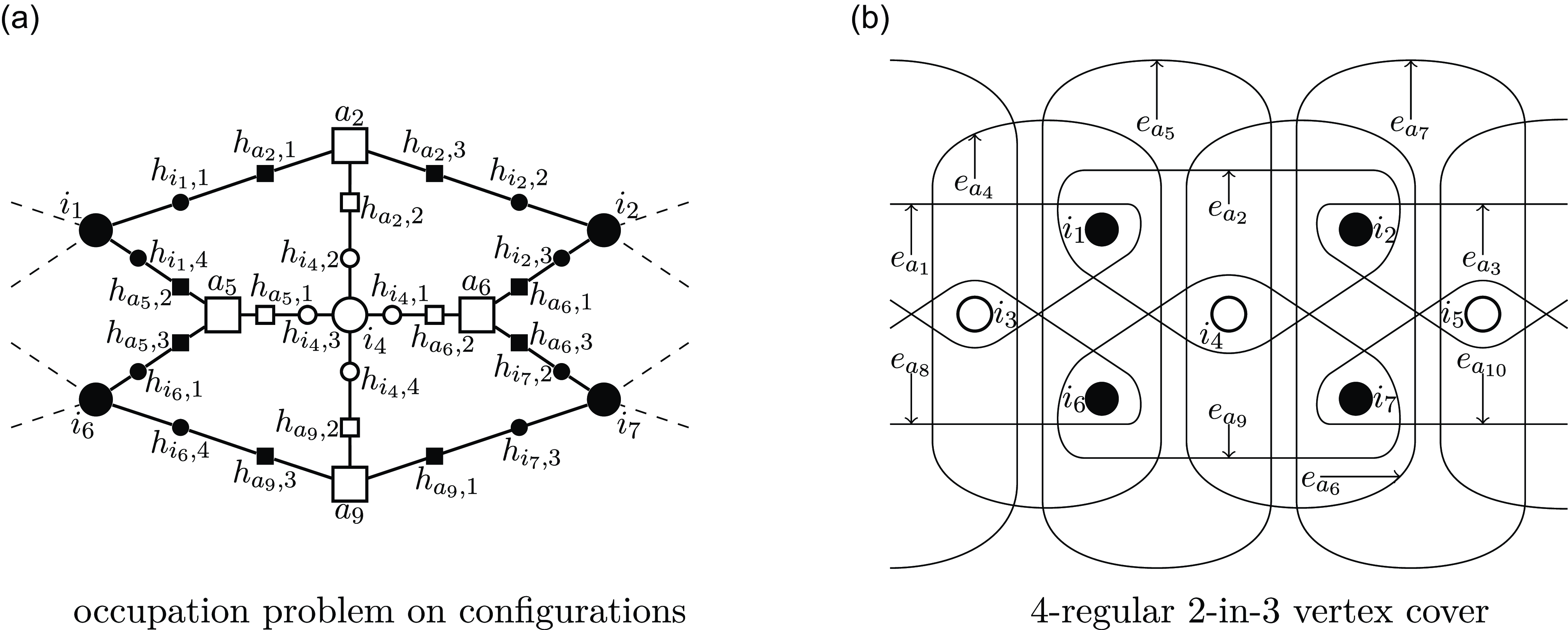
. Figure 1a shows an example of a
$o$
. Figure 1a shows an example of a $4$
-regular
$4$
-regular $2$
-in-
$2$
-in- $3$
occupation problem.
$3$
occupation problem.
Further, for given $m$
,
$m$
, $n\in \mathbb {Z}_{\gt 0}$
let
$n\in \mathbb {Z}_{\gt 0}$
let $\mathcal{O}$
denote the set of all instances
$\mathcal{O}$
denote the set of all instances $o$
with variables
$o$
with variables $V=[n]$
and constraints
$V=[n]$
and constraints $F=[m]$
. If
$F=[m]$
. If $\mathcal{O}$
is not empty, then the random
$\mathcal{O}$
is not empty, then the random $d$
-regular
$d$
-regular $r$
-in-
$r$
-in- $k$
occupation problem
$k$
occupation problem $O$
is uniform on
$O$
is uniform on $\mathcal{O}$
and
$\mathcal{O}$
and $Z=z(O)$
the number of solutions of
$Z=z(O)$
the number of solutions of $O$
.
$O$
.
1.3 Examples and related problems
On the left we see a solution of the $4$
-regular
$4$
-regular $2$
-in-
$2$
-in- $3$
occupation problem on a
$3$
occupation problem on a $4$
-regular
$4$
-regular $3$
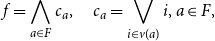
-factor graph, where the rectangles and circles depict the constraints (factors) and variables (filled if they take the value one in the solution). The figure on the right shows a
$3$
-factor graph, where the rectangles and circles depict the constraints (factors) and variables (filled if they take the value one in the solution). The figure on the right shows a $2$
-factor in a
$2$
-factor in a $3$
-regular
$3$
-regular $4$
-uniform hypergraph, where the circles, solid and dashed shapes represent the vertices, hyperedges in the
$4$
-uniform hypergraph, where the circles, solid and dashed shapes represent the vertices, hyperedges in the $2$
-factor and the other hyperedges respectively.
$2$
-factor and the other hyperedges respectively.
A problem that is closely related and can be reduced to the $d$
-regular
$d$
-regular $r$
-in-
$r$
-in- $k$
occupation problem is the
$k$
occupation problem is the $d$
-regular positive
$d$
-regular positive $r$
-in-
$r$
-in- $k$
SAT problem, a variant of
$k$
SAT problem, a variant of $k$
-SAT. We consider a Boolean formula
$k$
-SAT. We consider a Boolean formula
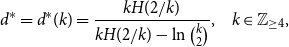
 \begin{align*} f=\bigwedge _{a\in F}c_a\textrm {, } \quad c_a=\bigvee _{i\in v(a)}i\textrm {, }a\in F\textrm {, } \end{align*}
in conjunctive normal form with $m$
clauses over
$m$
clauses over $n$
variables
$n$
variables $i\in V$
, such that no literal appears negated (hence positive
$i\in V$
, such that no literal appears negated (hence positive $r$
-in-
$r$
-in- $k$
SAT), and where each clause
$k$
SAT), and where each clause $c_a$
is the disjunction of
$c_a$
is the disjunction of $k$
literals and each variable appears in exactly
$k$
literals and each variable appears in exactly $d$
clauses (hence
$d$
clauses (hence $d$
-regular). The decision problem is to determine if there exists an assignment
$d$
-regular). The decision problem is to determine if there exists an assignment $x$
such that exactly
$x$
such that exactly $r$
literals in each clause evaluate to true (hence
$r$
literals in each clause evaluate to true (hence $r$
-in-
$r$
-in- $k$
SAT). In [Reference Moore34] the satisfiability threshold for this problem was determined for
$k$
SAT). In [Reference Moore34] the satisfiability threshold for this problem was determined for $r=1$
, i.e. the case where exactly one literal in each clause evaluates to true. Our Theorem1.1 solves this problem for
$r=1$
, i.e. the case where exactly one literal in each clause evaluates to true. Our Theorem1.1 solves this problem for $r=2$
and
$r=2$
and $k\in \mathbb {Z}_{\ge 4}$
.
$k\in \mathbb {Z}_{\ge 4}$
.
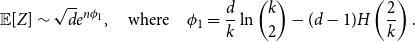
Our second example deals with a problem from graph theory.A $k$
-regular
$k$
-regular $d$
-uniform hypergraph
$d$
-uniform hypergraph $h$
is a pair
$h$
is a pair $h=(F,E)$
with
$h=(F,E)$
with $m = |F|$
vertices and
$m = |F|$
vertices and $n = |E|$
(hyper-)edges such that each edge contains
$n = |E|$
(hyper-)edges such that each edge contains $d$
vertices and the degree of each vertex is
$d$
vertices and the degree of each vertex is $k$
. An
$k$
. An $r$
-factor
$r$
-factor $E^{\prime}$
is a subset of the hyperedges such that each vertex
$E^{\prime}$
is a subset of the hyperedges such that each vertex $a\in F$
is incident to
$a\in F$
is incident to $r$
hyperedges
$r$
hyperedges $e_i\in E^{\prime}$
. In this case the problem is to determine if
$e_i\in E^{\prime}$
. In this case the problem is to determine if $h$
has an
$h$
has an $r$
-factor. For example, the case
$r$
-factor. For example, the case $r=1$
is the well-known perfect matching problem and the threshold was determined in [Reference Cooper, Frieze, Molloy and Reed11]. An example of a
$r=1$
is the well-known perfect matching problem and the threshold was determined in [Reference Cooper, Frieze, Molloy and Reed11]. An example of a $2$
-factor in a hypergraph is shown in Figure 1b. Theorem1.1 solves also this problem for
$2$
-factor in a hypergraph is shown in Figure 1b. Theorem1.1 solves also this problem for $r=2$
and
$r=2$
and $k\in \mathbb {Z}_{\ge 4}$
.
$k\in \mathbb {Z}_{\ge 4}$
.
Several other problems in complexity and graph theory are closely related to the examples above. The satisfiability threshold in Theorem1.1 also applies to a variant of the vertex cover problem (or hitting set problem from set theory perspective), where we choose a subset of the vertices (variables with value one) in a $d$
-regular
$d$
-regular $k$
-uniform hypergraph such that each hyperedge is incident to exactly two vertices in the subset. Analogously, Theorem1.1 also establishes the threshold for a variant of the set cover problem in set theory corresponding to
$k$
-uniform hypergraph such that each hyperedge is incident to exactly two vertices in the subset. Analogously, Theorem1.1 also establishes the threshold for a variant of the set cover problem in set theory corresponding to $2$
-factors in hypergraphs, i.e. given a family of
$2$
-factors in hypergraphs, i.e. given a family of $d$
-subsets (hyperedges) and a universe (vertices) with each element contained in
$d$
-subsets (hyperedges) and a universe (vertices) with each element contained in $k$
subsets, the problem is to find a subfamily of the subsets such that each element of the universe is contained in exactly two subsets of the subfamily. Further, Theorem1.1 can, e.g. also be used to give sufficient conditions for the (asymptotic) existence of Euler families in regular uniform hypergraphs as discussed in [Reference Bahmanian and Šajna2].
$k$
subsets, the problem is to find a subfamily of the subsets such that each element of the universe is contained in exactly two subsets of the subfamily. Further, Theorem1.1 can, e.g. also be used to give sufficient conditions for the (asymptotic) existence of Euler families in regular uniform hypergraphs as discussed in [Reference Bahmanian and Šajna2].
1.4 Main results
The satisfiability threshold for the $d$
-regular
$d$
-regular $1$
-in-
$1$
-in- $k$
occupation problem has been established in [Reference Cooper, Frieze, Molloy and Reed11, Reference Moore34], which also covers the
$k$
occupation problem has been established in [Reference Cooper, Frieze, Molloy and Reed11, Reference Moore34], which also covers the $d$
-regular
$d$
-regular $2$
-in-
$2$
-in- $3$
occupation problem due to colour symmetry. Our main result pins down the location of the satisfiability threshold of the random
$3$
occupation problem due to colour symmetry. Our main result pins down the location of the satisfiability threshold of the random $d$
-regular
$d$
-regular $2$
-in-
$2$
-in- $k$
occupation problem for
$k$
occupation problem for $k\in \mathbb {Z}_{\ge 4}$
. For this purpose let
$k\in \mathbb {Z}_{\ge 4}$
. For this purpose let
 \begin{align} d^*=d^*(k)=\frac {kH(2/k)}{kH(2/k)-\ln \binom {k}{2}}\textrm {,} \quad k\in \mathbb {Z}_{\ge 4}\textrm {,} \end{align}
where $H(p)=-p\ln (p)-(1-p)\ln (1-p)$
is the entropy of
$H(p)=-p\ln (p)-(1-p)\ln (1-p)$
is the entropy of $p\in [0,1]$
. The following theorem establishes the location of the threshold at
$p\in [0,1]$
. The following theorem establishes the location of the threshold at $d^*$
.
$d^*$
.
Theorem 1.1 ( $2$
-in-
$2$
-in- $k$
Occupation Satisfiability Threshold). Let
$k$
Occupation Satisfiability Threshold). Let $k\in \mathbb {Z}_{\ge 4}$
,
$k\in \mathbb {Z}_{\ge 4}$
, $d\in \mathbb {Z}_{\ge 2}$
, and let
$d\in \mathbb {Z}_{\ge 2}$
, and let $Z$
be the number of solutions from Section
1.1
. There exists a sharp satisfiability threshold at
$Z$
be the number of solutions from Section
1.1
. There exists a sharp satisfiability threshold at $d^*$
, i.e. for any increasing sequence
$d^*$
, i.e. for any increasing sequence $(n_i)_{i\in \mathbb {Z}_{\gt 0}}\subseteq \mathcal N=\{n:dn\textrm {, }2n\in k\mathbb {Z}_{\gt 0}\}$
and
$(n_i)_{i\in \mathbb {Z}_{\gt 0}}\subseteq \mathcal N=\{n:dn\textrm {, }2n\in k\mathbb {Z}_{\gt 0}\}$
and $m_i=dn_i/k$
we have
$m_i=dn_i/k$
we have
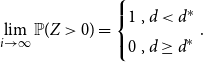 \begin{align*} \lim _{i\rightarrow \infty }\mathbb {P}(Z\gt 0)= \left \{\begin{matrix} 1&\textrm {, }d\lt d^*\\ 0&\textrm {, }d\ge d^* \end{matrix}\right .\textrm {.} \end{align*}
We provide a self-contained proof for Theorem 1.1 using the first and second moment method with small subgraph conditioning for $Z$
. In particular, a main technical contribution in proving Theorem1.1 is the optimization of a certain multivariate function that appears in the computation of the second moment, which encodes the interplay between the ‘similarity’ of various assignments and the change in the corresponding probability of being satisfying that they induce. A direct corollary of this optimization step at the threshold
$Z$
. In particular, a main technical contribution in proving Theorem1.1 is the optimization of a certain multivariate function that appears in the computation of the second moment, which encodes the interplay between the ‘similarity’ of various assignments and the change in the corresponding probability of being satisfying that they induce. A direct corollary of this optimization step at the threshold $d^*$
is the confirmation of the conjecture by the authors in [Reference Panagiotou and Pasch36]. Among other things, at the core of our contribution we take a novel and rather different approach to tackle the optimization, inspired by [Reference Robalewska37] and [Reference Yedidia, Freeman and Weiss41] as well as other works relating the fixed points of belief propagation to the stationary points of the Bethe free entropy, respectively to the computation of the annealed free entropy density; see Section 5.6 for details. Finally, we show that
$d^*$
is the confirmation of the conjecture by the authors in [Reference Panagiotou and Pasch36]. Among other things, at the core of our contribution we take a novel and rather different approach to tackle the optimization, inspired by [Reference Robalewska37] and [Reference Yedidia, Freeman and Weiss41] as well as other works relating the fixed points of belief propagation to the stationary points of the Bethe free entropy, respectively to the computation of the annealed free entropy density; see Section 5.6 for details. Finally, we show that $d^*$
is not an integer in Lemma 3.1 below, so as opposed to the case
$d^*$
is not an integer in Lemma 3.1 below, so as opposed to the case $r=1$
[Reference Moore34], for
$r=1$
[Reference Moore34], for $r=2$
there is no need for a dedicated analysis at criticality.
$r=2$
there is no need for a dedicated analysis at criticality.
1.5 Related work
The regular version of the random $1$
-in-
$1$
-in- $k$
occupation problem (and related problems) has been studied in [Reference Cooper, Frieze, Molloy and Reed11, Reference Moore34] using the first and second moment method with small subgraph conditioning. The paper [Reference Robalewska37] shows that
$k$
occupation problem (and related problems) has been studied in [Reference Cooper, Frieze, Molloy and Reed11, Reference Moore34] using the first and second moment method with small subgraph conditioning. The paper [Reference Robalewska37] shows that $\lim _{i\rightarrow \infty }\mathbb {P}(Z\gt 0)=1$
for
$\lim _{i\rightarrow \infty }\mathbb {P}(Z\gt 0)=1$
for $d=2$
and
$d=2$
and $k\in \mathbb {Z}_{\ge 2}$
in the
$k\in \mathbb {Z}_{\ge 2}$
in the $d$
-regular
$d$
-regular $2$
-in-
$2$
-in- $k$
occupation problem, i.e. the existence of
$k$
occupation problem, i.e. the existence of $2$
-factors in
$2$
-factors in $k$
-regular simple graphs. A recent discussion of
$k$
-regular simple graphs. A recent discussion of $2$
-factors (and the related Euler families) that does not rely on the probabilistic method is presented in [Reference Bahmanian and Šajna2]. Further, randomized polynomial time algorithms for the generation and approximate counting of
$2$
-factors (and the related Euler families) that does not rely on the probabilistic method is presented in [Reference Bahmanian and Šajna2]. Further, randomized polynomial time algorithms for the generation and approximate counting of $2$
-factors in random regular graphs have been developed in [Reference Frieze, Jerrum, Molloy, Robinson and Wormald19].
$2$
-factors in random regular graphs have been developed in [Reference Frieze, Jerrum, Molloy, Robinson and Wormald19].
The study of Erdős-Rényi (hyper-)graphs was initiated by the groundbreaking paper [Reference Erdős and Rényi16] in 1960 and turned into a fruitful field of research with many applications, including early results on $1$
-factors in simple graphs [Reference Erdős and Rényi17]. On the contrary, results for the random
$1$
-factors in simple graphs [Reference Erdős and Rényi17]. On the contrary, results for the random $d$
-regular
$d$
-regular $k$
-uniform (hyper-)graph ensemble were rare before the introduction of the configuration (or pairing) model by Bollobás [Reference Bollobás4] and the development of the small subgraph conditioning method [Reference Janson23, Reference Janson, Łuczak and Rucinski24]. While the proof scheme facilitated rigorous arguments to establish the existence and location of satisfiability thresholds of random regular CSPs [Reference Bapst, Coja-Oghlan and Efthymiou3, Reference Coja-Oghlan7, Reference Coja-Oghlan and Panagiotou10, Reference Ding, Sly and Sun14, Reference Ding, Sly and Sun15, Reference Kemkes, Pérez-Giménez and Wormald27, Reference Molloy, Robalewska, Robinson and Wormald33], the problems are treated on a case by case basis, while results on entire classes of random regular CSPs are still outstanding.
$k$
-uniform (hyper-)graph ensemble were rare before the introduction of the configuration (or pairing) model by Bollobás [Reference Bollobás4] and the development of the small subgraph conditioning method [Reference Janson23, Reference Janson, Łuczak and Rucinski24]. While the proof scheme facilitated rigorous arguments to establish the existence and location of satisfiability thresholds of random regular CSPs [Reference Bapst, Coja-Oghlan and Efthymiou3, Reference Coja-Oghlan7, Reference Coja-Oghlan and Panagiotou10, Reference Ding, Sly and Sun14, Reference Ding, Sly and Sun15, Reference Kemkes, Pérez-Giménez and Wormald27, Reference Molloy, Robalewska, Robinson and Wormald33], the problems are treated on a case by case basis, while results on entire classes of random regular CSPs are still outstanding.
One of the main reasons responsible for the complexity of a rigorous analysis of random (regular) CSPs seems to be a conjectured structural change of the solution space for increasing densities. This hypothesis has been put forward by physicists, verified in parts and mostly for ER ensembles, further led to new rigorous proof techniques [Reference Coja-Oghlan, Efthymiou, Jaafari, Kang and Kapetanopoulos8, Reference Coja-Oghlan and Panagiotou10, Reference Ding, Sly and Sun13] and to randomized algorithms [Reference Braunstein, Mézard and Zecchina5, Reference Maneva, Mossel and Wainwright30] for NP-hard problems that are not only of great value in practice, but can also be employed for precise numerical (though non-rigorous) estimates of satisfiability thresholds. An excellent introduction to this replica theory can be found in [Reference Krzakala, Ricci-Tersenghi, Zdeborová, Zecchina, Tramel and Cugliandolo28, Reference Mézard and Montanari31, Reference Talagrand40]. Specifically, numerical results indicating the satisfiability thresholds for $d$
-regular
$d$
-regular $r$
-in-
$r$
-in- $k$
occupation problems (more general variants, and for ER type hypergraphs) based on this conjecture were discussed in various publications [Reference Castellani, Napolano, Ricci-Tersenghi and Zecchina6, Reference Dall’Asta, Ramezanpour and Zecchina12, Reference Gabrié, Dani, Semerjian and Zdeborová20, Reference Higuchi and Mézard22, Reference Schmidt, Guenther and Zdeborová39, Reference Zdeborová and Krzakala42, Reference Zdeborová and Mézard43], where occupation problems were introduced for the first time in [Reference Mora35].
$k$
occupation problems (more general variants, and for ER type hypergraphs) based on this conjecture were discussed in various publications [Reference Castellani, Napolano, Ricci-Tersenghi and Zecchina6, Reference Dall’Asta, Ramezanpour and Zecchina12, Reference Gabrié, Dani, Semerjian and Zdeborová20, Reference Higuchi and Mézard22, Reference Schmidt, Guenther and Zdeborová39, Reference Zdeborová and Krzakala42, Reference Zdeborová and Mézard43], where occupation problems were introduced for the first time in [Reference Mora35].
Another fundamental obstacle in the rigorous analysis is of a very technical nature and directly related to the second moment method as discussed in detail in our current work. In the case of regular $2$
-in-
$2$
-in- $k$
occupation problems (amongst others) this optimization problem can be solved by exploiting a connection to the fixed points of belief propagation. This well-studied message passing algorithm is thoroughly discussed in [Reference Mézard and Montanari31].
$k$
occupation problems (amongst others) this optimization problem can be solved by exploiting a connection to the fixed points of belief propagation. This well-studied message passing algorithm is thoroughly discussed in [Reference Mézard and Montanari31].
1.6 Open problems
In this work we rigorously establish the threshold for $r=2$
and
$r=2$
and $k\in \mathbb {Z}_{\ge 4}$
for the random regular
$k\in \mathbb {Z}_{\ge 4}$
for the random regular $r$
-in-
$r$
-in- $k$
occupation problem. A rigorous proof for general
$k$
occupation problem. A rigorous proof for general $r$
(and
$r$
(and $k$
) seems to be involved, but further assumptions may significantly simplify the analysis. For example, as an extension of the current work one may focus on
$k$
) seems to be involved, but further assumptions may significantly simplify the analysis. For example, as an extension of the current work one may focus on $r$
-in-
$r$
-in- $2r$
occupation problems, where the constraints are symmetric in the colours. As can be seen from our proof, this yields useful symmetry properties. Further, as suggested by the literature [Reference Coja-Oghlan, Efthymiou, Jaafari, Kang and Kapetanopoulos8, Reference Coja-Oghlan, Krzakala, Perkins and Zdeborova9] such balanced problems [Reference Zdeborová and Krzakala42, Reference Zdeborová and Mézard43] are usually more accessible to a rigorous study. On the other hand, the optimization usually also significantly simplifies if only carried out for
$2r$
occupation problems, where the constraints are symmetric in the colours. As can be seen from our proof, this yields useful symmetry properties. Further, as suggested by the literature [Reference Coja-Oghlan, Efthymiou, Jaafari, Kang and Kapetanopoulos8, Reference Coja-Oghlan, Krzakala, Perkins and Zdeborova9] such balanced problems [Reference Zdeborová and Krzakala42, Reference Zdeborová and Mézard43] are usually more accessible to a rigorous study. On the other hand, the optimization usually also significantly simplifies if only carried out for $k\ge k_0(r)$
for some (large)
$k\ge k_0(r)$
for some (large) $k_0(r)$
.
$k_0(r)$
.
Apart from the generalizations discussed above, results for the general $r$
-in-
$r$
-in- $k$
occupation problems are also still outstanding for Erdős-Rényi type CSPs, the only exception being the satisfiability threshold for perfect matchings which was recently established by Kahn [Reference Kahn25]. Further, there only exist bounds for the exact cover problem [Reference Kalapala and Moore26] on
$k$
occupation problems are also still outstanding for Erdős-Rényi type CSPs, the only exception being the satisfiability threshold for perfect matchings which was recently established by Kahn [Reference Kahn25]. Further, there only exist bounds for the exact cover problem [Reference Kalapala and Moore26] on $3$
-uniform hypergraphs, i.e.
$3$
-uniform hypergraphs, i.e. $r=1$
and
$r=1$
and $k=3$
.
$k=3$
.
1.7 Outline of the Proofs
In Section 2 we present the proof strategy on a high level. Then, we turn to the notation and do some groundwork, in particular the analysis of $d^*(k)$
, in Section 3. The easy part of the main result is established in Section 4 using the first moment method. The remainder is devoted to the proof that solutions exist below the threshold with probability tending to one, starting with the second moment method in Section 5. Most of the twenty pages in this section are devoted to the solution of the optimization problem and related conjecture from [Reference Panagiotou and Pasch36] using a belief propagation inspired approach.
$d^*(k)$
, in Section 3. The easy part of the main result is established in Section 4 using the first moment method. The remainder is devoted to the proof that solutions exist below the threshold with probability tending to one, starting with the second moment method in Section 5. Most of the twenty pages in this section are devoted to the solution of the optimization problem and related conjecture from [Reference Panagiotou and Pasch36] using a belief propagation inspired approach.
Finally, we complete the small subgraph conditioning method in Section 6, using the proof of Lemma 2.8 in Appendix A as a blueprint.
2. Proof techniques
In this section we give a high-level overview of our proof. We make heavy use of the so-called configuration model for the generation of random instances in the form used by Moore [Reference Moore34].
2.1 The configuration model
Working with the uniform distribution on $d$
-regular
$d$
-regular $k$
-uniform hypergraphs directly is challenging. Instead, we show Theorem1.1 for occupation problems on so-called configurations. A
$k$
-uniform hypergraphs directly is challenging. Instead, we show Theorem1.1 for occupation problems on so-called configurations. A $d$
-regular
$d$
-regular $k$
-configuration is a bijection
$k$
-configuration is a bijection $g:[n]\times [d]\rightarrow [m]\times [k]$
, where the v-edges
$g:[n]\times [d]\rightarrow [m]\times [k]$
, where the v-edges $(i,h^{\prime})\in [n]\times [d]$
represent pairs of variables
$(i,h^{\prime})\in [n]\times [d]$
represent pairs of variables $i\in [n]$
and so-called
$i\in [n]$
and so-called $i$
-edges, i.e. half-edge indices
$i$
-edges, i.e. half-edge indices $h^{\prime}\in [d]$
. The image
$h^{\prime}\in [d]$
. The image $(a,h)=g(i,h^{\prime})$
is an f-edge, i.e. a pair of a constraint (factor)
$(a,h)=g(i,h^{\prime})$
is an f-edge, i.e. a pair of a constraint (factor) $a\in [m]$
and an
$a\in [m]$
and an $a$
-edge (or half-edge)
$a$
-edge (or half-edge) $h\in [k]$
, indicating that the
$h\in [k]$
, indicating that the $i$
-edge
$i$
-edge $h^{\prime}$
of the variable
$h^{\prime}$
of the variable $i$
is wired to the
$i$
is wired to the $a$
-edge
$a$
-edge $h$
of
$h$
of $a$
and thereby suggesting that
$a$
and thereby suggesting that $i$
is connected to
$i$
is connected to $a$
in the corresponding
$a$
in the corresponding $d$
-regular
$d$
-regular $k$
-factor graph. Notice that we can represent
$k$
-factor graph. Notice that we can represent $g$
by an equivalent, four-partite, graph with (disjoint) vertex sets given by the variables
$g$
by an equivalent, four-partite, graph with (disjoint) vertex sets given by the variables $V=[n]$
, constraints (factors)
$V=[n]$
, constraints (factors) $F=[m]$
, v-edges
$F=[m]$
, v-edges $H^{\prime}=[n]\times [d]$
and f-edges
$H^{\prime}=[n]\times [d]$
and f-edges $H=[m]\times [k]$
, where each variable
$H=[m]\times [k]$
, where each variable $i\in [n]$
connects to all its v-edges
$i\in [n]$
connects to all its v-edges $(i,h^{\prime})\in H^{\prime}$
, each constraint
$(i,h^{\prime})\in H^{\prime}$
, each constraint $a\in [m]$
to all its f-edges
$a\in [m]$
to all its f-edges $(a,h)\in H$
and a v-edge
$(a,h)\in H$
and a v-edge $(i,h^{\prime})$
connects to an f-edge
$(i,h^{\prime})$
connects to an f-edge $(a,h)$
if
$(a,h)$
if $g(i,h^{\prime})=(a,h)$
.
$g(i,h^{\prime})=(a,h)$
.
Let $\mathcal{G}$
be the set of all
$\mathcal{G}$
be the set of all $d$
-regular
$d$
-regular $k$
-configurations on
$k$
-configurations on $n$
variables, and notice that
$n$
variables, and notice that $|\mathcal{G}|=\emptyset$
iff
$|\mathcal{G}|=\emptyset$
iff $dn\neq km$
and
$dn\neq km$
and $|\mathcal{G}|=(dn)!=(km)!$
for
$|\mathcal{G}|=(dn)!=(km)!$
for $m=dn/k\in \mathbb {Z}$
, which we assume from here on. Further, the occupation problem on factor graphs directly translates to configurations, i.e. an assignment
$m=dn/k\in \mathbb {Z}$
, which we assume from here on. Further, the occupation problem on factor graphs directly translates to configurations, i.e. an assignment $x\in \{0,1\}^n$
is a solution of
$x\in \{0,1\}^n$
is a solution of $g\in \mathcal{G}$
if for each constraint
$g\in \mathcal{G}$
if for each constraint $a\in [m]$
there exist exactly two distinct
$a\in [m]$
there exist exactly two distinct $a$
-edges
$a$
-edges $h$
,
$h$
, $h^{\prime}\in [k]$
such that
$h^{\prime}\in [k]$
such that $x_{i(a,h)}=x_{i(a,h^{\prime})}=1$
, where
$x_{i(a,h)}=x_{i(a,h^{\prime})}=1$
, where $i(a,h)=(g^{-1}(a,h))_1$
denotes the
$i(a,h)=(g^{-1}(a,h))_1$
denotes the $h$
-th neighbour of
$h$
-th neighbour of $a$
. Say, the occupation problem on a configuration corresponding to the example in Figure 1a is shown in Figure 2a.
$a$
. Say, the occupation problem on a configuration corresponding to the example in Figure 1a is shown in Figure 2a.
Let $Z(g)$
be the number of solutions of
$Z(g)$
be the number of solutions of $g \in \mathcal{G}$
. As before,
$g \in \mathcal{G}$
. As before, $Z=0$
almost surely unless
$Z=0$
almost surely unless $2n\in k\mathbb {Z}$
. Theorem1.1 is a straightforward consequence of the following result.
$2n\in k\mathbb {Z}$
. Theorem1.1 is a straightforward consequence of the following result.
Theorem 2.1 (Satisfiability Threshold for Configurations). Theorem
1.1
also holds for $Z$
as defined in this section.
$Z$
as defined in this section.
Theorem2.1 translates to the models in Section 1.1 and Section 1.2 using standard arguments, namely symmetry, the discussion of parallel edges, contiguity, and the fact that both the variable and the factor neighbourhoods are unique with probability tending to one. Hence, in the remainder of this contribution we exclusively consider the occupation problem on configurations.
The figure on the left shows the solution on a configuration corresponding to the solution in Figure 1. We only denoted $a$
-edges (small boxes, filled if they the
$a$
-edges (small boxes, filled if they the $a$
-edge takes the value one) and
$a$
-edge takes the value one) and $i$
-edges (small circles, filled if the
$i$
-edges (small circles, filled if the $i$
-edge takes the value one) instead of f-edges and v-edges for brevity (e.g.
$i$
-edge takes the value one) instead of f-edges and v-edges for brevity (e.g. $h_{a_1,1}$
instead of
$h_{a_1,1}$
instead of $(a_1,h_{a_1,1})$
).The figure on the right illustrates the corresponding
$(a_1,h_{a_1,1})$
).The figure on the right illustrates the corresponding $2$
-in-
$2$
-in- $3$
vertex cover (given by the filled circles).
$3$
vertex cover (given by the filled circles).
2.2 The first moment method
In the first step we apply the first moment method to the occupation problem on configurations, yielding the following result.
Lemma 2.2 (First Moment Method). Let $k\in \mathbb {Z}_{\ge 4}$
,
$k\in \mathbb {Z}_{\ge 4}$
, $d\in \mathbb {Z}_{\ge 2}$
. For
$d\in \mathbb {Z}_{\ge 2}$
. For $n\in \mathcal N$
tending to infinity
$n\in \mathcal N$
tending to infinity
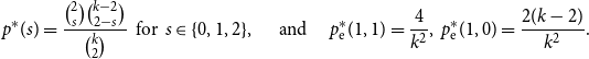
 \begin{align*} \mathbb {E}[Z]&\sim \sqrt {d}e^{n\phi _1}, \quad \textrm {where} \quad \phi _1=\frac {d}{k}\ln \binom {k}{2}-(d-1)H\left (\frac 2k\right ) \textrm {.} \end{align*}
In particular, $\mathbb {E}[Z]\rightarrow \infty$
for
$\mathbb {E}[Z]\rightarrow \infty$
for $d\lt d^*$
and
$d\lt d^*$
and $\mathbb {E}[Z]\rightarrow 0$
for
$\mathbb {E}[Z]\rightarrow 0$
for $d\gt d^*$
with
$d\gt d^*$
with $d^*$
as in (1). So, Markov’s inequality implies
$d^*$
as in (1). So, Markov’s inequality implies $\mathbb {P}(Z\gt 0)\rightarrow 0$
for
$\mathbb {P}(Z\gt 0)\rightarrow 0$
for $d\gt d^*$
. The map
$d\gt d^*$
. The map $\phi _1$
is known as annealed free entropy density.
$\phi _1$
is known as annealed free entropy density.
2.3 The second moment method
Let $k\in \mathbb {Z}_{\ge 4}$
and
$k\in \mathbb {Z}_{\ge 4}$
and $d\in \mathbb {Z}_{\ge 2}$
. We denote the set of distributions on a finite set
$d\in \mathbb {Z}_{\ge 2}$
. We denote the set of distributions on a finite set $\mathcal S$
by
$\mathcal S$
by $\mathcal P(\mathcal S)$
and identify
$\mathcal P(\mathcal S)$
and identify $p\in \mathcal P(\mathcal S)$
with its probability mass function, meaning
$p\in \mathcal P(\mathcal S)$
with its probability mass function, meaning $\mathcal P(\mathcal S)=\{p\in [0,1]^{\mathcal S}:\sum _{x\in \mathcal S}p(s)=1\}$
. Further, let
$\mathcal P(\mathcal S)=\{p\in [0,1]^{\mathcal S}:\sum _{x\in \mathcal S}p(s)=1\}$
. Further, let $\mathcal P_{\ell }(\mathcal S)=\{p\in \mathcal P(\mathcal S):\ell p\in \mathbb {Z}^{\mathcal S}\}$
be the empirical distributions over
$\mathcal P_{\ell }(\mathcal S)=\{p\in \mathcal P(\mathcal S):\ell p\in \mathbb {Z}^{\mathcal S}\}$
be the empirical distributions over $\ell \in \mathbb {Z}_{\gt 0}$
trials.
$\ell \in \mathbb {Z}_{\gt 0}$
trials.
In order to apply the second moment method we will consider a (new) CSP with $m$
factors on
$m$
factors on $n$
variables with the larger domain
$n$
variables with the larger domain $\{0,1\}^2$
, and where the constraint
$\{0,1\}^2$
, and where the constraint $a\in [m]$
is satisfied by an assignment
$a\in [m]$
is satisfied by an assignment $x\in (\{0,1\}^2)^n$
if
$x\in (\{0,1\}^2)^n$
if $\sum _{i\in v(a)}x_{i,1}=\sum _{i\in v(a)}x_{i,2}=2$
. Here, there are qualitatively three types of satisfying assignments for the constraints, namely with
$\sum _{i\in v(a)}x_{i,1}=\sum _{i\in v(a)}x_{i,2}=2$
. Here, there are qualitatively three types of satisfying assignments for the constraints, namely with $0$
,
$0$
, $1$
or
$1$
or $2$
overlapping ones. We will analyse the empirical overlap distributions
$2$
overlapping ones. We will analyse the empirical overlap distributions $p\in \mathcal P_m(\{0,1,2\})$
of assignments satisfying all constraints, which determine the empirical distributions
$p\in \mathcal P_m(\{0,1,2\})$
of assignments satisfying all constraints, which determine the empirical distributions $p_{\mathrm {e}}\in \mathcal P_{km}(\{0,1\}^2)$
of the values
$p_{\mathrm {e}}\in \mathcal P_{km}(\{0,1\}^2)$
of the values $\{0,1\}^2$
over the
$\{0,1\}^2$
over the $km$
edges, given by
$km$
edges, given by
 \begin{align*} p_{\mathrm {e}}(11)=\frac {1}{k}p(1)+\frac {2}{k}p(2) \,\,\textrm { and } \,\, p_{\mathrm {e}}(10)=p_{\mathrm {e}}(01)=\frac {1}{k}p(1)+\frac {2}{k}p(0)\textrm {.} \end{align*}
So, if $p\in \mathcal P_m(\{0,1,2\})$
is an achievable empirical overlap distribution on the
$p\in \mathcal P_m(\{0,1,2\})$
is an achievable empirical overlap distribution on the $m$
factors, then
$m$
factors, then $p_{\mathrm {e}}$
is necessarily an empirical distribution on the
$p_{\mathrm {e}}$
is necessarily an empirical distribution on the $n$
variables; thus the achievable overlap distributions are contained in
$n$
variables; thus the achievable overlap distributions are contained in $\mathcal P_n=\left \{p\in \mathcal P_m(\{0,1,2\})\,:\,p_{\mathrm {e}}\in \mathcal P_n(\{0,1\}^2)\right \}$
.
$\mathcal P_n=\left \{p\in \mathcal P_m(\{0,1,2\})\,:\,p_{\mathrm {e}}\in \mathcal P_n(\{0,1\}^2)\right \}$
.
In the first – combinatorial – part we establish that the second moment can be written as a sum of all contributions over all achievable overlap distributions.
Lemma 2.3 (Second Moment Combinatorics). For any $n\in \mathcal N$
we have
$n\in \mathcal N$
we have
 \begin{align*} \mathbb {E}[Z^2]=\sum _{p \in \mathcal P_n}E(p), \text { where } E(p)=\binom {m}{mp}\prod _{s\in \{0,1,2\}}\binom {k}{s,2-s,2-s,k-4+s}^{mp(s)}\binom {n}{np_{\mathrm {e}}}\binom {dn}{dnp_{\mathrm {e}}}^{-1}\textrm {.} \end{align*}
Here, we use the notation $\binom {m}{mp}$
,
$\binom {m}{mp}$
, $p\in \mathcal P_m(\{0,1,2\})$
, for multinomial coefficients.
$p\in \mathcal P_m(\{0,1,2\})$
, for multinomial coefficients.
To study further the second moment in Lemma 2.3, we identify the maximal contributions. For this purpose, let $p^*\in \mathcal P(\{0,1,2\})$
be the hypergeometric distribution with
$p^*\in \mathcal P(\{0,1,2\})$
be the hypergeometric distribution with
 \begin{align} p^*(s)=\frac {\binom {2}{s}\binom {k-2}{2-s}}{\binom {k}{2}} \, \textrm { for }\, s\in \{0,1,2\}, \quad \textrm { and }\quad p^*_{\mathrm {e}}(1,1)=\frac {4}{k^2}, \, p^*_{\mathrm {e}}(1,0)=\frac {2(k-2)}{k^2}\textrm {.} \end{align}
The overlap distribution $p^*$
is a natural candidate for maximizing
$p^*$
is a natural candidate for maximizing $E(p)$
. Indeed, we obtain
$E(p)$
. Indeed, we obtain $p^*$
when we consider two independent uniformly random assignments in
$p^*$
when we consider two independent uniformly random assignments in $\{0,1\}^k$
with
$\{0,1\}^k$
with $2$
ones each, and
$2$
ones each, and $p^*_{\mathrm {e}}$
is exactly the marginal probability if we jointly consider two independent uniformly random assignments in
$p^*_{\mathrm {e}}$
is exactly the marginal probability if we jointly consider two independent uniformly random assignments in $\{0,1\}^n$
to the variables with
$\{0,1\}^n$
to the variables with $2n/k$
ones each. In the next step, we derive the limits of the log-densities
$2n/k$
ones each. In the next step, we derive the limits of the log-densities $\frac {1}{n}\ln (E(p))$
. Recall that the K(ullback)-L(eibler) divergence
$\frac {1}{n}\ln (E(p))$
. Recall that the K(ullback)-L(eibler) divergence $D_{\textrm {KL}}(p\parallel q)$
of two distributions
$D_{\textrm {KL}}(p\parallel q)$
of two distributions $p$
,
$p$
, $q\in \mathcal P(\mathcal S)$
, such that
$q\in \mathcal P(\mathcal S)$
, such that $p$
is absolutely continuous with respect to
$p$
is absolutely continuous with respect to $q$
, is
$q$
, is
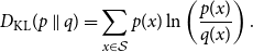 \begin{align*} D_{\textrm {KL}}(p\parallel q)=\sum _{x\in \mathcal S}p(x)\ln \left (\frac {p(x)}{q(x)}\right )\textrm {.} \end{align*}
Lemma 2.4 (Second Moment Asymptotics). For any fully supported $p\in \mathcal P(\{0,1,2\})$
and any sequence
$p\in \mathcal P(\{0,1,2\})$
and any sequence $(p_n)_{n\in \mathcal N}\subseteq \mathcal P_n$
with
$(p_n)_{n\in \mathcal N}\subseteq \mathcal P_n$
with $\lim _{n\rightarrow \infty }p_n=p$
we have
$\lim _{n\rightarrow \infty }p_n=p$
we have $\lim _{n\rightarrow \infty }\frac {1}{n}\ln (E(p_n))=\phi _2(p)$
, where
$\lim _{n\rightarrow \infty }\frac {1}{n}\ln (E(p_n))=\phi _2(p)$
, where
 \begin{align*} \phi _2(p)=2\phi _1-\frac {d}{k}\Delta _d(p) \quad \text {and} \quad \Delta _d(p)=D_{\textrm {KL}}(p\parallel p^*)-\frac {(d-1)k}{d}D_{\textrm {KL}} (p_{\mathrm {e}}\parallel p^*_{\mathrm {e}})\textrm {.} \end{align*}
The following proposition is the main contribution of this work.
Proposition 2.5 (Second Moment Minimizers). For $k=4$
the global minimizers of
$k=4$
the global minimizers of $\Delta _{d^*(4)}$
are
$\Delta _{d^*(4)}$
are $p^*$
,
$p^*$
, $p^{(0)}$
given by
$p^{(0)}$
given by $p^{(0)}(0)=1$
and
$p^{(0)}(0)=1$
and $p^{(2)}$
given by
$p^{(2)}$
given by $p^{(2)}(2)=1$
. For
$p^{(2)}(2)=1$
. For $k\in \mathbb {Z}_{\ge 5}$
the global minimizers of
$k\in \mathbb {Z}_{\ge 5}$
the global minimizers of $\Delta _{d^*(k)}$
are
$\Delta _{d^*(k)}$
are $p^*$
and
$p^*$
and $p^{(2)}$
.
$p^{(2)}$
.
With Proposition 2.5, we easily verify that $p^*$
is the unique minimizer of
$p^*$
is the unique minimizer of $\Delta _d$
for any
$\Delta _d$
for any $d\lt d^*(k)$
, since the KL divergence is minimized by its unique root and
$d\lt d^*(k)$
, since the KL divergence is minimized by its unique root and $(d-1)k/d$
is increasing in
$(d-1)k/d$
is increasing in $d$
. This conclusion then allows us to compute the limit of the scaled second moment using Laplace’s method for sums. More than that, we confirm the conjecture by the authors in [Reference Panagiotou and Pasch36] as an immediate corollary.
$d$
. This conclusion then allows us to compute the limit of the scaled second moment using Laplace’s method for sums. More than that, we confirm the conjecture by the authors in [Reference Panagiotou and Pasch36] as an immediate corollary.
Proposition 2.6 (Second Moment Limit). For any $k\in \mathbb {Z}_{\ge 4}$
and
$k\in \mathbb {Z}_{\ge 4}$
and $d\lt d^*(k)$
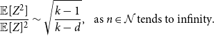 \begin{align*} \frac {\mathbb {E}[Z^2]}{\mathbb {E}[Z]^2}&\sim \sqrt {\frac {k-1}{k-d}},\,\,\textrm { as }n\in \mathcal N\textrm { tends to infinity.} \end{align*}
Proposition 2.6 and the Paley-Zygmund inequality yield $\textrm {lim inf}_{n\rightarrow \infty }\mathbb {P}(Z\gt 0)\ge \sqrt {\frac {k-d}{k-1}}$
. While this bound suggests that a threshold exists, we need to show that the threshold at
$\textrm {lim inf}_{n\rightarrow \infty }\mathbb {P}(Z\gt 0)\ge \sqrt {\frac {k-d}{k-1}}$
. While this bound suggests that a threshold exists, we need to show that the threshold at $d^*$
is sharp.
$d^*$
is sharp.
2.4 Small subgraph conditioning
We complete the proof of Theorem2.1 using the small subgraph conditioning method. For this purpose let $a^{\underline {b}}=\prod _{c=0}^{b-1}(a-c)$
denote the falling factorial.
$a^{\underline {b}}=\prod _{c=0}^{b-1}(a-c)$
denote the falling factorial.
Theorem 2.7 (Small Subgraph Conditioning, [Reference Moore34, Theorem 2]). Let $Z_n$
and
$Z_n$
and $X_{n,1},X_{n,2},\ldots$
be non-negative integer-valued random variables. Suppose that
$X_{n,1},X_{n,2},\ldots$
be non-negative integer-valued random variables. Suppose that $\mathbb {E}[Z_n]\gt 0$
and that for each
$\mathbb {E}[Z_n]\gt 0$
and that for each $\ell \in \mathbb {Z}_{\gt 0}$
there are
$\ell \in \mathbb {Z}_{\gt 0}$
there are $\lambda _\ell \in \mathbb {R}_{\gt 0}$
,
$\lambda _\ell \in \mathbb {R}_{\gt 0}$
, $\delta _\ell \in \mathbb {R}_{\gt -1}$
such that for any
$\delta _\ell \in \mathbb {R}_{\gt -1}$
such that for any $L\in \mathbb {Z}_{\gt 0}$
-
a) the variables $X_{n,1},\ldots, X_{n,L}$
are asymptotically independent and Poisson with
$\mathbb {E}[X_{n,\ell }]\sim \lambda _\ell$
,
$X_{n,1},\ldots, X_{n,L}$
are asymptotically independent and Poisson with
$\mathbb {E}[X_{n,\ell }]\sim \lambda _\ell$
, -
b) for any sequence
$r_1,\ldots, r_{L}$
of non-negative integers,
\begin{align*} \frac {\mathbb {E}\left [Z_n\prod _{\ell =1}^{L}X_{n,\ell }^{\underline {r_\ell }}\right ]}{\mathbb {E}[Z_n]}\sim \prod _{\ell =1}^{L}[\lambda _\ell (1+\delta _\ell )]^{r_\ell }, \end{align*}
-
c) we explain the variance, i.e.
\begin{align*} \frac {\mathbb {E}[Z_n^2]}{\mathbb {E}[Z_n]^2}\sim \exp \left (\sum _{\ell \ge 1}\lambda _\ell \delta _\ell ^2\right ) \quad \textrm { and }\quad \sum _{\ell \ge 1}\lambda _\ell \delta _\ell ^2\lt \infty \textrm {.} \end{align*}


Then $\lim _{n\rightarrow \infty }\mathbb {P}(Z_n \gt 0)=1$
.
$\lim _{n\rightarrow \infty }\mathbb {P}(Z_n \gt 0)=1$
.
We will apply Theorem 2.7 to the number $Z$
of solutions from Section 2.1 and the numbers
$Z$
of solutions from Section 2.1 and the numbers $X_\ell$
of small cycles in the configuration
$X_\ell$
of small cycles in the configuration $G$
. In order to understand what a cycle in a configuration is, we recall the representation of a configuration
$G$
. In order to understand what a cycle in a configuration is, we recall the representation of a configuration $g$
as a four-partite graph from Section 2.1.
$g$
as a four-partite graph from Section 2.1.
Since we are mostly interested in the factor graph associated with a configuration we divide the lengths of paths by three, e.g. what we call a cycle of length four in the bijection, is actually a cycle of length twelve in its equivalent four-partite graph representation. Figures 1a and 2a show an example of a factor graph and the corresponding configuration in its graph representation. Showing the following statement, which establishes Assumption2.7a), is rather routine.
Lemma 2.8 (Small Cycles). For $\ell \in \mathbb {Z}_{\gt 0}$
let
$\ell \in \mathbb {Z}_{\gt 0}$
let $X_\ell$
be the number of
$X_\ell$
be the number of $2\ell$
-cycles in
$2\ell$
-cycles in $G$
, and set
$G$
, and set
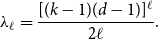 \begin{align*} \lambda _\ell =\frac {[(k-1)(d-1)]^\ell }{2\ell }. \end{align*}
Then $X_1,\ldots, X_{L}$
are asymptotically independent and Poisson with
$X_1,\ldots, X_{L}$
are asymptotically independent and Poisson with $\mathbb {E}[X_\ell ]\sim \lambda _\ell$
for all
$\mathbb {E}[X_\ell ]\sim \lambda _\ell$
for all $L\in \mathbb {Z}_{\gt 0}$
.
$L\in \mathbb {Z}_{\gt 0}$
.
We give a self-contained proof of Lemma 2.8 in the appendix, which we build upon to argue that Assumption2.7b) in Theorem2.7 holds. With Lemma 2.8 in place, we consider the base case in Assumption2.7b), i.e. for $\ell \in \mathbb {Z}_{\gt 0}$
we let
$\ell \in \mathbb {Z}_{\gt 0}$
we let $r_\ell =1$
and
$r_\ell =1$
and $r_{\ell ^{\prime}}=0$
otherwise, to determine
$r_{\ell ^{\prime}}=0$
otherwise, to determine $\delta _\ell =(1-k)^{-\ell }$
. We easily verify that
$\delta _\ell =(1-k)^{-\ell }$
. We easily verify that $\sum _{\ell \ge 1}\lambda _\ell \delta _\ell ^2=\frac 12\ln (\frac {k-1}{k-d})$
and thereby establish Assumption2.7c) using Proposition 2.6. Finally, we follow the proof of Lemma 2.8 to complete the verification of Assumption2.7b) and thereby complete the proof of Theorem1.1.
$\sum _{\ell \ge 1}\lambda _\ell \delta _\ell ^2=\frac 12\ln (\frac {k-1}{k-d})$
and thereby establish Assumption2.7c) using Proposition 2.6. Finally, we follow the proof of Lemma 2.8 to complete the verification of Assumption2.7b) and thereby complete the proof of Theorem1.1.
3. Preliminaries and notation
After introducing notation in Section 3.1, we establish a few basic facts in Section 3.2.
3.1 Notation
We use the notation $[n]=\{1,\ldots, n\}$
and
$[n]=\{1,\ldots, n\}$
and $[n]_0=\{0\}\cup [n]$
for
$[n]_0=\{0\}\cup [n]$
for $n\in \mathbb {Z}_{\gt 0}$
, denote the falling factorial with
$n\in \mathbb {Z}_{\gt 0}$
, denote the falling factorial with $n^{\underline {k}}$
for
$n^{\underline {k}}$
for $n,k\in \mathbb {Z}_{\ge 0}$
,
$n,k\in \mathbb {Z}_{\ge 0}$
, $k\le n$
, and multinomial coefficients with
$k\le n$
, and multinomial coefficients with $\binom {n}{k}$
for
$\binom {n}{k}$
for $n\in \mathbb {Z}_{\ge 0}$
and
$n\in \mathbb {Z}_{\ge 0}$
and $k\in \mathbb {Z}_{\ge 0}^d$
,
$k\in \mathbb {Z}_{\ge 0}^d$
, $d\in \mathbb {Z}_{\gt 1}$
, such that
$d\in \mathbb {Z}_{\gt 1}$
, such that $\sum _{i\in [d]}k_i=n$
. For functions
$\sum _{i\in [d]}k_i=n$
. For functions $f$
,
$f$
, $g$
on integers with
$g$
on integers with $\lim _{n\rightarrow \infty }{f(n)}/{g(n)}=1$
we write
$\lim _{n\rightarrow \infty }{f(n)}/{g(n)}=1$
we write $f(n)\sim g(n)$
. We make heavy use of Stirling’s formula [Reference Robbins38], i.e.
$f(n)\sim g(n)$
. We make heavy use of Stirling’s formula [Reference Robbins38], i.e.
 \begin{align*} \sqrt {2\pi n}\left (\frac {n}{e}\right )^ne^{\frac {1}{12n+1}}\le n!\le \sqrt {2\pi n}\left (\frac {n}{e}\right )^ne^{\frac {1}{12n}}, \quad n\in \mathbb {Z}_{\gt 0}, \end{align*}
and in particular $n!\sim \sqrt {2\pi n}(\frac {n}{e})^n$
. If a random variable
$n!\sim \sqrt {2\pi n}(\frac {n}{e})^n$
. If a random variable $X$
has law
$X$
has law $P$
we write
$P$
we write $X\sim P$
and use
$X\sim P$
and use $\textrm {Po}(\lambda )$
to denote the Poisson distribution with parameter
$\textrm {Po}(\lambda )$
to denote the Poisson distribution with parameter $\lambda$
. Distributions
$\lambda$
. Distributions $p\in \mathcal P(\mathcal S)$
in the convex polytope
$p\in \mathcal P(\mathcal S)$
in the convex polytope $\mathcal P(\mathcal S)$
of distributions with finite support
$\mathcal P(\mathcal S)$
of distributions with finite support $\mathcal S$
are identified with their probability mass functions
$\mathcal S$
are identified with their probability mass functions $p\in [0,1]^{\mathcal S}$
. Further,
$p\in [0,1]^{\mathcal S}$
. Further, $\mathcal P_n(\mathcal S)=\{p\in \mathcal P(\mathcal S)\,:\,np\in [n]_0\}$
denotes the set of empirical distributions obtained from
$\mathcal P_n(\mathcal S)=\{p\in \mathcal P(\mathcal S)\,:\,np\in [n]_0\}$
denotes the set of empirical distributions obtained from $n\in \mathbb {Z}_{\ge 1}$
trials. Let
$n\in \mathbb {Z}_{\ge 1}$
trials. Let $v^{\mathrm {t}}$
denote the transpose of a vector
$v^{\mathrm {t}}$
denote the transpose of a vector $v$
. Finally, we use ‘iff’ for ‘if and only if’.
$v$
. Finally, we use ‘iff’ for ‘if and only if’.
3.2 Basic observations
We briefly establish the claims in Section 1.1 for the configuration version, and the claim that $d^*$
is not an integer.
$d^*$
is not an integer.
Lemma 3.1.
The set $\mathcal{G}$
is empty iff
$\mathcal{G}$
is empty iff $dn\neq km$
, so let
$dn\neq km$
, so let $dn=km$
. Then, we have
$dn=km$
. Then, we have $Z=0$
almost surely if
$Z=0$
almost surely if $n_1=2n/k\not \in \mathbb {Z}$
. Finally,
$n_1=2n/k\not \in \mathbb {Z}$
. Finally, $d^*\in (1,\infty )\setminus \mathbb {Z}$
.
$d^*\in (1,\infty )\setminus \mathbb {Z}$
.
Proof. Since $g\in \mathcal{G}$
is a bijection
$g\in \mathcal{G}$
is a bijection $g:[n]\times [d]\rightarrow [m]\times [k]$
, the set
$g:[n]\times [d]\rightarrow [m]\times [k]$
, the set $\mathcal{G}$
is empty for
$\mathcal{G}$
is empty for $dn\neq km$
and
$dn\neq km$
and $|\mathcal{G}|=(dn)!=(km)!$
otherwise, which proves the first assertion. Next, we fix a solution
$|\mathcal{G}|=(dn)!=(km)!$
otherwise, which proves the first assertion. Next, we fix a solution $x\in \{0,1\}^n$
of
$x\in \{0,1\}^n$
of $g\in \mathcal{G}$
with
$g\in \mathcal{G}$
with $n^{\prime}_1$
ones. Then two
$n^{\prime}_1$
ones. Then two $a$
-edges
$a$
-edges $h$
have to take the value one, i.e.
$h$
have to take the value one, i.e. $x_{i(a,h)}=1$
, for each
$x_{i(a,h)}=1$
, for each $a\in [m]$
and hence
$a\in [m]$
and hence $2m$
f-edges
$2m$
f-edges $(a,h)\in [m]\times [k]$
in total. On the other hand, there are
$(a,h)\in [m]\times [k]$
in total. On the other hand, there are $dn^{\prime}_1$
v-edges
$dn^{\prime}_1$
v-edges $(i,h)\in [n]\times [d]$
that take the value one. Since
$(i,h)\in [n]\times [d]$
that take the value one. Since $g$
is a bijection,
$g$
is a bijection, $dn^{\prime}_1=2m$
, so
$dn^{\prime}_1=2m$
, so $n_1=n^{\prime}_1\in \mathbb {Z}$
.
$n_1=n^{\prime}_1\in \mathbb {Z}$
.
For the last assertion, we first focus on the denominator of $d^*$
, i.e.
$d^*$
, i.e.
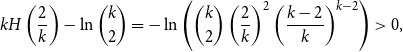 \begin{align*} kH\left (\frac {2}{k}\right )-\ln \binom {k}{2}=-\ln \left (\binom {k}{2}\left (\frac {2}{k}\right )^2\left (\frac {k-2}{k}\right )^{k-2}\right )\gt 0\textrm {,} \end{align*}
so $d^*\gt 0$
for
$d^*\gt 0$
for $k\in \mathbb {Z}_{\ge 3}$
. Next, notice that
$k\in \mathbb {Z}_{\ge 3}$
. Next, notice that $d^*$
is a solution of
$d^*$
is a solution of $f(d)=1$
with
$f(d)=1$
with
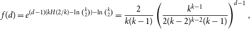 \begin{align*} f(d)=e^{(d-1)(kH(2/k)-\ln \binom {k}{2})-\ln \binom {k}{2}}=\frac {2}{k(k-1)}\left (\frac {k^{k-1}}{2(k-2)^{k-2}(k-1)}\right )^{d-1}\textrm {,} \end{align*}
which directly implies that $d^*\gt 1$
and further, since
$d^*\gt 1$
and further, since $\gcd (k,k-1)=1$
, that
$\gcd (k,k-1)=1$
, that $d^*\in (1,\infty )\setminus \mathbb {Z}$
.
$d^*\in (1,\infty )\setminus \mathbb {Z}$
.
4. The first moment method – proof of Lemma 2.2
This short section is dedicated to the proof of Lemma 2.2. We write the expectation in terms of the number $|\mathcal{E}|$
of pairs
$|\mathcal{E}|$
of pairs $(g,x)\in \mathcal{E}$
such that
$(g,x)\in \mathcal{E}$
such that $x\in \{0,1\}^n$
satisfies
$x\in \{0,1\}^n$
satisfies $g\in \mathcal{G}$
, i.e.
$g\in \mathcal{G}$
, i.e.
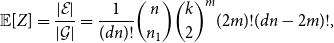 \begin{align*} \mathbb {E}[Z] =\frac {|\mathcal{E}|}{|\mathcal{G}|} =\frac {1}{(dn)!}\binom {n}{n_1}\binom {k}{2}^m(2m)!(dn-2m)!\textrm {,} \end{align*}
with $n_1=2n/k$
and for the following reasons. First, we choose the
$n_1=2n/k$
and for the following reasons. First, we choose the $n_1$
variables with value one in
$n_1$
variables with value one in $x$
, then we choose the two
$x$
, then we choose the two $a$
-edges for each constraint
$a$
-edges for each constraint $a\in [m]$
with value one, wire the v-edges and f-edges with value one and finally wire the edges with value zero. In particular, this implies that
$a\in [m]$
with value one, wire the v-edges and f-edges with value one and finally wire the edges with value zero. In particular, this implies that $\mathbb {E}[Z]\gt 0$
for all
$\mathbb {E}[Z]\gt 0$
for all $n\in \mathcal N$
.
$n\in \mathcal N$
.
Using Stirling’s formula, the asymptotics are given by
 \begin{align*} \mathbb {E}[Z] &=\frac {\binom {n}{n_1}\binom {k}{2}^m}{\binom {km}{2m}} \sim \sqrt {\frac {2\pi km\frac 2k(1-\frac 2k)}{2\pi n\frac 2k(1-\frac 2k)}}\exp \left (nH\left (\frac 2k\right )-kmH\left (\frac 2k\right )+m\ln \left (\binom k2\right )\right ) =\sqrt {d}e^{n\phi _1}. \end{align*}
5. The second moment method
In this section we consider the case $d\lt d^*$
. We prove Lemma 2.3, Lemma 2.4, Proposition 2.5 and Proposition 2.6, the main contribution of this work.
$d\lt d^*$
. We prove Lemma 2.3, Lemma 2.4, Proposition 2.5 and Proposition 2.6, the main contribution of this work.
5.1 How to square a constraint satisfaction problem
In order to facilitate the presentation we introduce the squared $d$
-regular
$d$
-regular $2$
-in-
$2$
-in- $k$
occupation problem. As before, an instance of this problem is given by a bijection
$k$
occupation problem. As before, an instance of this problem is given by a bijection $g\,:\,[n]\times [d]\rightarrow [m]\times [k]$
. Now, for an assignment
$g\,:\,[n]\times [d]\rightarrow [m]\times [k]$
. Now, for an assignment $x\in (\{0,1\}^2)^n$
let
$x\in (\{0,1\}^2)^n$
let $y_{g,x}=(x_{i(a,h)})_{a\in [m],h\in [k]}$
be the corresponding f-edge assignment under
$y_{g,x}=(x_{i(a,h)})_{a\in [m],h\in [k]}$
be the corresponding f-edge assignment under $g$
, where we recall from Section 2.1 that
$g$
, where we recall from Section 2.1 that $i(a,h)=(g^{-1}(a,h))_1\in [n]$
is the variable
$i(a,h)=(g^{-1}(a,h))_1\in [n]$
is the variable $i(a,h)$
wired to the f-edge
$i(a,h)$
wired to the f-edge $(a,h)$
under
$(a,h)$
under $g$
. A constraint
$g$
. A constraint $a\in [m]$
is satisfied by a constraint assignment
$a\in [m]$
is satisfied by a constraint assignment $x\in (\{0,1\}^2)^k$
iff
$x\in (\{0,1\}^2)^k$
iff $x\in \mathcal S^{(2)}$
, where
$x\in \mathcal S^{(2)}$
, where
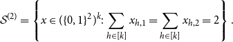 \begin{align*} \mathcal S^{(2)} =\left \{x\in (\{0,1\}^2)^k:\sum _{h\in [k]}x_{h,1}=\sum _{h\in [k]}x_{h,2}=2\right \}\textrm {.} \end{align*}
An f-edge assignment $x\in (\{0,1\}^2)^{m\times k}$
is satisfying if
$x\in (\{0,1\}^2)^{m\times k}$
is satisfying if $x_a=(x_{a,h})_{h\in [k]}$
satisfies
$x_a=(x_{a,h})_{h\in [k]}$
satisfies $a$
for all
$a$
for all $a\in [m]$
. Finally, an assignment
$a\in [m]$
. Finally, an assignment $x\in (\{0,1\}^2)^n$
is a solution of
$x\in (\{0,1\}^2)^n$
is a solution of $g$
if
$g$
if $y_{g,x}$
is satisfying. Notice that the pairs of solutions
$y_{g,x}$
is satisfying. Notice that the pairs of solutions $x$
,
$x$
, $x^{\prime}\in \{0,1\}^n$
of the standard problem on
$x^{\prime}\in \{0,1\}^n$
of the standard problem on $g$
are in one to one correspondence with the solutions
$g$
are in one to one correspondence with the solutions $y\in (\{0,1\}^2)^n$
of the squared problem on
$y\in (\{0,1\}^2)^n$
of the squared problem on $g$
via
$g$
via $y=(x_i,x^{\prime}_i)_{i\in [n]}$
. So,
$y=(x_i,x^{\prime}_i)_{i\in [n]}$
. So, $z^{(2)}(g)=z(g)^2$
for the number
$z^{(2)}(g)=z(g)^2$
for the number $z^{(2)}(g)$
of solutions of the squared problem, hence
$z^{(2)}(g)$
of solutions of the squared problem, hence $Z^{(2)}=Z^2$
for
$Z^{(2)}=Z^2$
for $Z^{(2)}=z^{(2)}(G)$
and in particular
$Z^{(2)}=z^{(2)}(G)$
and in particular $\mathbb {E}[Z^{(2)}]=\mathbb {E}[Z^2]$
. This equivalence allows us to entirely focus on the squared problem.
$\mathbb {E}[Z^{(2)}]=\mathbb {E}[Z^2]$
. This equivalence allows us to entirely focus on the squared problem.
5.2 Proof of Lemma 2.3
As before, we can write $\mathbb {E}[Z^{(2)}]=\frac {1}{(dn)!}|\mathcal{E}|$
, where
$\mathbb {E}[Z^{(2)}]=\frac {1}{(dn)!}|\mathcal{E}|$
, where $|\mathcal{E}|$
is the number of pairs
$|\mathcal{E}|$
is the number of pairs $(g,x)\in \mathcal{E}$
such that
$(g,x)\in \mathcal{E}$
such that $x\in (\{0,1\}^2)^n$
solves
$x\in (\{0,1\}^2)^n$
solves $g$
. Set
$g$
. Set
 \begin{align*} \mathcal Y=\left \{y\in (\{0,1\}^2)^{m\times k}\,:\,y_a\in \mathcal S^{(2)} \,\textrm {for all}\,a\in [m]\right \}. \end{align*}
For $y\in \mathcal Y$
let the overlap distribution
$y\in \mathcal Y$
let the overlap distribution $p_y\in \mathcal P_m(\{0,1,2\})$
be given by
$p_y\in \mathcal P_m(\{0,1,2\})$
be given by
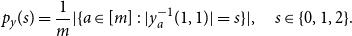 \begin{align*} p_y(s)=\frac {1}{m}|\{a\in [m]\,:\,|y_a^{-1}(1,1)|=s\}|, \quad s\in \{0,1,2\}. \end{align*}
Further, let the edge distribution $q_y\in \mathcal P_{km}(\{0,1\}^2)$
be given by
$q_y\in \mathcal P_{km}(\{0,1\}^2)$
be given by
 \begin{align*} q_y(x)=\frac {1}{km}|\{(a,h)\in [m]\times [k]\,:\,y_{a,h}=x\}|=\frac {1}{km}|y^{-1}(x)|,\quad x\in \{0,1\}^2\textrm {.} \end{align*}
Using that $|y_a^{-1}(1,0)|=|y_a^{-1}(0,1)|=2-|y_a^{-1}(1,1)|$
and hence
$|y_a^{-1}(1,0)|=|y_a^{-1}(0,1)|=2-|y_a^{-1}(1,1)|$
and hence $|y^{-1}(0,0)|=k-4+|y^{-1}(1,1)|$
we directly get
$|y^{-1}(0,0)|=k-4+|y^{-1}(1,1)|$
we directly get
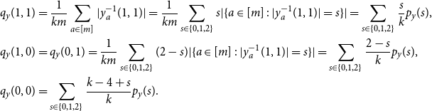 \begin{align*} q_y(1,1)&=\frac {1}{km}\sum _{a\in [m]}|y_a^{-1}(1,1)|=\frac {1}{km}\sum _{s\in \{0,1,2\}}s|\{a\in [m]\,:\,|y_a^{-1}(1,1)|=s\}|=\sum _{s\in \{0,1,2\}}\frac {s}{k}p_y(s)\textrm {,}\\ q_y(1,0)&=q_y(0,1)=\frac {1}{km}\sum _{s\in \{0,1,2\}}(2-s)|\{a\in [m]\,:\,|y_a^{-1}(1,1)|=s\}|=\sum _{s\in \{0,1,2\}}\frac {2-s}{k}p_y(s)\textrm {,}\\ q_y(0,0)&=\sum _{s\in \{0,1,2\}}\frac {k-4+s}{k}p_y(s)\textrm {.} \end{align*}
Hence, let $p_{\mathrm {e}}=Wp\in \mathcal P(\{0,1\}^2)$
denote the edge distribution of any (not necessarily empirical) overlap distribution
$p_{\mathrm {e}}=Wp\in \mathcal P(\{0,1\}^2)$
denote the edge distribution of any (not necessarily empirical) overlap distribution $p\in \mathcal P(\{0,1,2\})$
, where
$p\in \mathcal P(\{0,1,2\})$
, where $W\in [0,1]^{\{0,1\}^2\times \{0,1,2\}}$
is given by
$W\in [0,1]^{\{0,1\}^2\times \{0,1,2\}}$
is given by
 \begin{align} W_{11,s}=\frac {s}{k}\textrm {, } \,\,W_{10,s}=W_{01,s}=\frac {2-s}{k} \,\textrm { and }\,W_{00,s}=\frac {k-4+s}{k}, \quad s\in \{0,1,2\}\textrm {.} \end{align}
Now, notice that for any $(g,x)\in \mathcal{E}$
we have
$(g,x)\in \mathcal{E}$
we have $y_{g,x,a,h}=x_{i(a,h)}$
for all
$y_{g,x,a,h}=x_{i(a,h)}$
for all $a\in [m]$
,
$a\in [m]$
, $h\in [k]$
, hence
$h\in [k]$
, hence $g(x^{-1}(z)\times [d])=y_{g,x}^{-1}(z)$
and by that
$g(x^{-1}(z)\times [d])=y_{g,x}^{-1}(z)$
and by that
 \begin{align*} q_{y_{g,x}}(z)=\frac {|y_{g,x}^{-1}(z)|}{km}=\frac {d|x^{-1}(z)|}{km}=\frac {1}{n}|x^{-1}(z)|=q_{x}(z)\textrm { for }z\in \{0,1\}^2\textrm {,} \end{align*}
i.e. the relative frequencies of the values in the f-edge assignment $y_{g,x}$
coincide with the relative frequencies
$y_{g,x}$
coincide with the relative frequencies $q_x\in \mathcal P_n(\{0,1\}^2)$
of the values in the variable assignment
$q_x\in \mathcal P_n(\{0,1\}^2)$
of the values in the variable assignment $x$
. In particular, this shows that a satisfying f-edge assignment
$x$
. In particular, this shows that a satisfying f-edge assignment $y\in \mathcal Y$
is only attainable if
$y\in \mathcal Y$
is only attainable if $q_y\in \mathcal P_n(\{0,1\}^2)$
, and thereby
$q_y\in \mathcal P_n(\{0,1\}^2)$
, and thereby
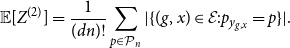 \begin{align*} \mathbb {E}[Z^{(2)}]=\frac {1}{(dn)!}\sum _{p\in \mathcal P_n}|\{(g,x)\in \mathcal{E}:p_{y_{g,x}}=p\}|. \end{align*}
Now, fix an attainable satisfying f-edge assignment $y\in \mathcal Y$
and an assignment
$y\in \mathcal Y$
and an assignment $x\in (\{0,1\}^2)^n$
with
$x\in (\{0,1\}^2)^n$
with $q_y=q_x$
, i.e.
$q_y=q_x$
, i.e. $|x^{-1}(z)\times [d]|=|y^{-1}(z)|$
for all
$|x^{-1}(z)\times [d]|=|y^{-1}(z)|$
for all $z\in \{0,1\}^2$
. Any bijection
$z\in \{0,1\}^2$
. Any bijection $g$
with
$g$
with $y=y_{g,x}$
needs to respect
$y=y_{g,x}$
needs to respect $g(x^{-1}(z)\times [d])=y_{g,x}^{-1}(z)$
for
$g(x^{-1}(z)\times [d])=y_{g,x}^{-1}(z)$
for $z\in \{0,1\}^2$
and can hence be uniquely decomposed into its restrictions
$z\in \{0,1\}^2$
and can hence be uniquely decomposed into its restrictions $g_z\,:\,x^{-1}(z)\times [d]\rightarrow y_{g,x}^{-1}(z)$
. On the other hand, any choice of such restrictions
$g_z\,:\,x^{-1}(z)\times [d]\rightarrow y_{g,x}^{-1}(z)$
. On the other hand, any choice of such restrictions $g_z$
gives a bijection
$g_z$
gives a bijection $g$
with
$g$
with $y=y_{g,x}$
, and so
$y=y_{g,x}$
, and so
 \begin{align*} |\mathcal{E}_{x,y}|&=\prod _{z\in \{0,1\}^2}(dnq_x(z))!=\prod _{z\in \{0,1\}^2}(dnp_{y,\mathrm {e}}(z))!\,\,\textrm {, where }\, \mathcal{E}_{x,y}=\{(g,x)\in \mathcal{E}:y_{g,x}=y\}\textrm {.} \end{align*}
Notice that $\mathcal{E}_{x,y}\cap \mathcal{E}_{x^{\prime},y^{\prime}}=\emptyset$
for any
$\mathcal{E}_{x,y}\cap \mathcal{E}_{x^{\prime},y^{\prime}}=\emptyset$
for any $(x,y)\neq (x^{\prime},y^{\prime})$
, which is obvious for
$(x,y)\neq (x^{\prime},y^{\prime})$
, which is obvious for $x\neq x^{\prime}$
, and also for
$x\neq x^{\prime}$
, and also for $y\neq y^{\prime}$
, since
$y\neq y^{\prime}$
, since $y_{g,x}=y\neq y^{\prime}=y_{g^{\prime},x}$
implies that
$y_{g,x}=y\neq y^{\prime}=y_{g^{\prime},x}$
implies that $g\neq g^{\prime}$
. But since
$g\neq g^{\prime}$
. But since $|\mathcal{E}_{x,y}|$
only depends on
$|\mathcal{E}_{x,y}|$
only depends on $p_{y}$
(actually only on
$p_{y}$
(actually only on $p_{y,\mathrm {e}}$
) this completes the proof, because for any fixed attainable overlap distribution
$p_{y,\mathrm {e}}$
) this completes the proof, because for any fixed attainable overlap distribution $p\in \mathcal P_n$
, we can now independently choose the satisfying f-edge assignment
$p\in \mathcal P_n$
, we can now independently choose the satisfying f-edge assignment $y$
and variable assignment
$y$
and variable assignment $x$
, subject to
$x$
, subject to $q_x=p_{\mathrm {e}}$
and
$q_x=p_{\mathrm {e}}$
and $p_y=p$
(which implies
$p_y=p$
(which implies $q_y=q_x$
). So we have
$q_y=q_x$
). So we have $\mathbb {E}[Z^{(2)}]=\sum _{p}E(p)$
with
$\mathbb {E}[Z^{(2)}]=\sum _{p}E(p)$
with $p\in \mathcal P_n$
and
$p\in \mathcal P_n$
and
 \begin{align*} E(p)=\frac {1}{(dn)!}\binom {n}{np_{\mathrm {e}}}\binom {m}{mp}\prod _{s\in \{0,1,2\}}\binom {k}{s,2-s,2-s,k-4+s}^{mp(s)}\prod _{x\in \{0,1\}^2}(dnp_{\mathrm {e}}(z))!\textrm {,} \end{align*}
where we choose a variable assignment $x$
with
$x$
with $q_x=p_{\mathrm {e}}$
, an f-edge assignment
$q_x=p_{\mathrm {e}}$
, an f-edge assignment $y$
with
$y$
with $p_y=p$
by first choosing one of the
$p_y=p$
by first choosing one of the $\binom {m}{mp}$
options for
$\binom {m}{mp}$
options for $(|y_a^{-1}(1,1)|)_{a\in [m]}$
and then independently one of the
$(|y_a^{-1}(1,1)|)_{a\in [m]}$
and then independently one of the $\binom {k}{s,2-s,2-s,k-4+s}$
satisfying constraint assignments for each of the
$\binom {k}{s,2-s,2-s,k-4+s}$
satisfying constraint assignments for each of the $mp(s)$
constraints with overlap
$mp(s)$
constraints with overlap $s\in \{0,1,2\}$
, and finally choosing a bijection
$s\in \{0,1,2\}$
, and finally choosing a bijection $g$
with
$g$
with $(g,x)\in \mathcal{E}_{x,y}$
.
$(g,x)\in \mathcal{E}_{x,y}$
.
5.3 Empirical overlap distributions
This section is dedicated to deriving properties of the set $\mathcal P_n$
for
$\mathcal P_n$
for $n\in \mathcal N$
. In the following we will use the canonical ascending order on
$n\in \mathcal N$
. In the following we will use the canonical ascending order on $\{0,1,2\}$
to denote points in
$\{0,1,2\}$
to denote points in $\mathbb {R}^{\{0,1,2\}}$
and the ascending lexicographical order on
$\mathbb {R}^{\{0,1,2\}}$
and the ascending lexicographical order on $\{0,1\}^2$
to denote points in
$\{0,1\}^2$
to denote points in $\mathbb {R}^{\{0,1\}^2}$
. Recall that
$\mathbb {R}^{\{0,1\}^2}$
. Recall that $p^{(s)}\in \mathcal P(\{0,1,2\})$
given by
$p^{(s)}\in \mathcal P(\{0,1,2\})$
given by $p^{(s)}(s)=1$
for
$p^{(s)}(s)=1$
for $s\in \{0,1,2\}$
denote the corners of the convex polytope
$s\in \{0,1,2\}$
denote the corners of the convex polytope $\mathcal P(\{0,1,2\})$
and further consider the vectors in
$\mathcal P(\{0,1,2\})$
and further consider the vectors in $\mathbb {R}^{\{0,1,2\}}$
 \begin{align} b_1=({-}d,d,0)^{\mathrm {t}}, \quad b_2=(1,-2,1)^{\mathrm {t}}. \end{align}
Finally, let
 \begin{align*} \mathcal X=\Big \{x\in \mathbb {R}^2\,:\,(b_1,b_2)x\ge -p^{(0)}\Big \},\quad \mathcal X_n=\mathcal X\cap (m^{-1}\mathbb {Z})^2. \end{align*}
Lemma 5.1.
The map $\iota _n\,:\,\mathcal X_n\rightarrow \mathcal P_n$
,
$\iota _n\,:\,\mathcal X_n\rightarrow \mathcal P_n$
, $x\mapsto p^{(0)}+(b_1,b_2)x$
is a bijection.
$x\mapsto p^{(0)}+(b_1,b_2)x$
is a bijection.
Proof.
We use the shorthands $1_{\{0,1,2\}}=(1)_{s\in \{0,1,2\}}$
and
$1_{\{0,1,2\}}=(1)_{s\in \{0,1,2\}}$
and
 \begin{align*} 1_{\{0,1,2\}}^{\perp }&=\left \{x\in \mathbb {R}^{\{0,1,2\}}:1_{\{0,1,2\}}^{\mathrm {t}}x=0\right \} =\left \{x\in \mathbb {R}^{\{0,1,2\}}:\sum _{s\in \{0,1,2\}}x_s=0\right \}. \end{align*}
Note that $\mathcal P(\{0,1,2\})\subseteq p^{(0)}+1_{\{0,1,2\}}^{\perp } = \{p^{(0)}+x:x\in 1_{\{0,1,2\}}^{\perp }\}$
. On the other hand,
$\mathcal P(\{0,1,2\})\subseteq p^{(0)}+1_{\{0,1,2\}}^{\perp } = \{p^{(0)}+x:x\in 1_{\{0,1,2\}}^{\perp }\}$
. On the other hand, $(b_1,b_2)$
is a basis of
$(b_1,b_2)$
is a basis of $1_{\{0,1,2\}}^{\perp }$
, and hence
$1_{\{0,1,2\}}^{\perp }$
, and hence
 \begin{equation} \iota \,:\,\mathbb {R}^2\rightarrow p^{(0)}+1_{\{0,1,2\}}^{\perp }, \quad x\mapsto p^{(0)}+(b_1,b_2)x, \end{equation}
is bijective. This gives that $\iota (\mathcal X)=\mathcal P(\{0,1,2\})$
and that
$\iota (\mathcal X)=\mathcal P(\{0,1,2\})$
and that $\iota _n$
is the restriction of
$\iota _n$
is the restriction of $\iota$
to
$\iota$
to $\mathcal X_n$
, so
$\mathcal X_n$
, so $\iota _n$
is a bijection from
$\iota _n$
is a bijection from $\mathcal X_n$
to
$\mathcal X_n$
to $\mathcal P(\{0,1,2\})\cap \iota \left ((m^{-1}\mathbb {Z})^2\right )$
. Consequently, it remains to show that
$\mathcal P(\{0,1,2\})\cap \iota \left ((m^{-1}\mathbb {Z})^2\right )$
. Consequently, it remains to show that $\mathcal P_n=\mathcal P(\{0,1,2\})\cap \iota \left ((m^{-1}\mathbb {Z})^2\right )$
, where
$\mathcal P_n=\mathcal P(\{0,1,2\})\cap \iota \left ((m^{-1}\mathbb {Z})^2\right )$
, where
 \begin{align*} \iota \left ((m^{-1}\mathbb {Z})^2\right )=\left \{p^{(0)}+\frac {i_1}{m}b_1+\frac {i_2}{m}b_2:i\in \mathbb {Z}^2\right \} \end{align*}
is a grid anchored at $p^{(0)}$
and spanned by
$p^{(0)}$
and spanned by $m^{-1}b_1$
and
$m^{-1}b_1$
and $m^{-1}b_2$
. Note that
$m^{-1}b_2$
. Note that
 \begin{align*} p^{(0)}_{\mathrm {e}}=\left (\frac {k-4}{k},\frac {2}{k},\frac {2}{k},0\right )^{\mathrm {t}}\textrm {,} \end{align*}
so $np^{(0)}_{\mathrm {e}}\in \mathbb {Z}^{\{0,1\}^2}$
since
$np^{(0)}_{\mathrm {e}}\in \mathbb {Z}^{\{0,1\}^2}$
since $n\in \mathcal N$
, and hence
$n\in \mathcal N$
, and hence $p^{(0)}\in \mathcal P_n$
by the definition of
$p^{(0)}\in \mathcal P_n$
by the definition of $\mathcal P_n$
. Next, we show that
$\mathcal P_n$
. Next, we show that $\mathcal P_n$
is on the grid, i.e.
$\mathcal P_n$
is on the grid, i.e. $\mathcal P_n\subseteq \iota \left ((m^{-1}\mathbb {Z})^2\right )$
. For this purpose fix
$\mathcal P_n\subseteq \iota \left ((m^{-1}\mathbb {Z})^2\right )$
. For this purpose fix $p\in \mathcal P_n$
and let
$p\in \mathcal P_n$
and let $x=\iota ^{-1}(p)$
, i.e.
$x=\iota ^{-1}(p)$
, i.e. $mp\in \mathbb {Z}^{\{0,1,2\}}$
,
$mp\in \mathbb {Z}^{\{0,1,2\}}$
, $n(Wp)\in \mathbb {Z}^{\{0,1\}^2}$
and
$n(Wp)\in \mathbb {Z}^{\{0,1\}^2}$
and $p=p^{(0)}+x_1b_1+x_2b_2$
. This directly gives
$p=p^{(0)}+x_1b_1+x_2b_2$
. This directly gives $mx_2=mp(2)\in \mathbb {Z}$
. Further, we notice that
$mx_2=mp(2)\in \mathbb {Z}$
. Further, we notice that $b_2$
is in the kernel of
$b_2$
is in the kernel of $W$
from Equation (3), i.e.
$W$
from Equation (3), i.e. $Wb_2=0_{\{0,1\}^2}$
, and
$Wb_2=0_{\{0,1\}^2}$
, and $Wb_1=\frac {d}{k}w$
with
$Wb_1=\frac {d}{k}w$
with $w=(1,-1,-1,1)^{\mathrm {t}}$
. This directly gives
$w=(1,-1,-1,1)^{\mathrm {t}}$
. This directly gives $p_{\mathrm {e}}(1,1)=0+\frac {d}{k}x_1+0$
and hence
$p_{\mathrm {e}}(1,1)=0+\frac {d}{k}x_1+0$
and hence $mx_1=np_{\mathrm {e}}(1,1)\in \mathbb {Z}$
, i.e.
$mx_1=np_{\mathrm {e}}(1,1)\in \mathbb {Z}$
, i.e. $x\in (m^{-1}\mathbb {Z})^2$
and hence
$x\in (m^{-1}\mathbb {Z})^2$
and hence $p=\iota (x)\in \iota \left ((m^{-1}\mathbb {Z})^2\right )$
. Conversely, for any
$p=\iota (x)\in \iota \left ((m^{-1}\mathbb {Z})^2\right )$
. Conversely, for any $x\in \mathcal X_n$
and with
$x\in \mathcal X_n$
and with $p=\iota (x)$
we have
$p=\iota (x)$
we have $p\in \mathcal P(\{0,1,2\})$
since
$p\in \mathcal P(\{0,1,2\})$
since $x\in \mathcal X$
, further
$x\in \mathcal X$
, further $mp=mp^{(0)}+(b_1,b_2)(mx)\in \mathbb {Z}^{\{0,1,2\}}$
since
$mp=mp^{(0)}+(b_1,b_2)(mx)\in \mathbb {Z}^{\{0,1,2\}}$
since $mx\in \mathbb {Z}^2$
and the other terms on the right-hand side are integer valued by definition, and finally
$mx\in \mathbb {Z}^2$
and the other terms on the right-hand side are integer valued by definition, and finally $np_{\mathrm {e}}=np^{(0)}_{\mathrm {e}}+mx_1w\in \mathbb {Z}^{\{0,1\}^2}$
.
$np_{\mathrm {e}}=np^{(0)}_{\mathrm {e}}+mx_1w\in \mathbb {Z}^{\{0,1\}^2}$
.
Using Lemma 5.1 we have $\mathbb {E}[Z^{(2)}]=\sum _{x\in \mathcal X_n}E(\iota _n(x))$
, where
$\mathbb {E}[Z^{(2)}]=\sum _{x\in \mathcal X_n}E(\iota _n(x))$
, where $\mathcal X_n\subseteq \mathbb {R}^2$
may be considered as a normalization of the grid
$\mathcal X_n\subseteq \mathbb {R}^2$
may be considered as a normalization of the grid $\mathcal P_n\subseteq p^{(0)}+1_{\{0,1,2\}}^{\mathrm {t}}$
. In order to prepare the upcoming asymptotics of the second moment, we give a complete characterization of the convex polytope
$\mathcal P_n\subseteq p^{(0)}+1_{\{0,1,2\}}^{\mathrm {t}}$
. In order to prepare the upcoming asymptotics of the second moment, we give a complete characterization of the convex polytope $\mathcal X$
and the image of
$\mathcal X$
and the image of $\mathcal X$
under
$\mathcal X$
under $W(b_1,b_2)$
, i.e. the image
$W(b_1,b_2)$
, i.e. the image $p_{\mathrm {e}}=Wp$
of
$p_{\mathrm {e}}=Wp$
of $p\in \mathcal P(\{0,1,2\})$
under
$p\in \mathcal P(\{0,1,2\})$
under $W$
from Equation (3). Let
$W$
from Equation (3). Let $w=(1,-1,-1,1)^{\mathrm {t}}$
from the proof of Lemma 5.1, and set
$w=(1,-1,-1,1)^{\mathrm {t}}$
from the proof of Lemma 5.1, and set
 \begin{align*} \mathcal W = \Big \{p^{(0)}_{\mathrm {e}}+yw\,:\,y\in [0,2/k]\Big \}\subseteq \mathcal P(\{0,1\}^2), \quad \mathcal X_p=\left \{x\in \mathcal X:x_1=\frac {k}{d}p(1,1)\right \} \text { for } p\in \mathcal W. \end{align*}
Moreover, recall the definition of $p^*$
from (2) and the bijection
$p^*$
from (2) and the bijection $\iota$
from (5), and let
$\iota$
from (5), and let
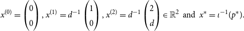 \begin{align*} x^{(0)}=\begin{pmatrix}0\\ 0\end{pmatrix}\textrm {, } x^{(1)}=d^{-1}\begin{pmatrix}1\\ 0\end{pmatrix}\textrm {, } x^{(2)}=d^{-1}\begin{pmatrix}2\\ d\end{pmatrix}\in \mathbb {R}^2\,\textrm { and }\, x^*=\iota ^{-1}(p^*)\textrm {.} \end{align*}
Lemma 5.2.
The set $\mathcal X$
is a two-dimensional convex polytope with corners
$\mathcal X$
is a two-dimensional convex polytope with corners $x^{(0)},x^{(1)},x^{(2)}$
, and
$x^{(0)},x^{(1)},x^{(2)}$
, and $x^*$
is in the interior of
$x^*$
is in the interior of $\mathcal X$
. The image of
$\mathcal X$
. The image of $\mathcal X$
under
$\mathcal X$
under $W(b_1,b_2)$
is the one-dimensional convex polytope
$W(b_1,b_2)$
is the one-dimensional convex polytope $\mathcal W$
with corners
$\mathcal W$
with corners $p^{(0)}_{\mathrm {e}}$
and
$p^{(0)}_{\mathrm {e}}$
and $p^{(2)}_{\mathrm {e}}$
. Further, the preimage of
$p^{(2)}_{\mathrm {e}}$
. Further, the preimage of $p\in \mathcal W$
under
$p\in \mathcal W$
under $W(b_1,b_2)$
is
$W(b_1,b_2)$
is $\mathcal X_p$
, where
$\mathcal X_p$
, where $\mathcal X_{p^{(s)}_{\mathrm {e}}}=\{p^{(s)}\}$
for
$\mathcal X_{p^{(s)}_{\mathrm {e}}}=\{p^{(s)}\}$
for $s\in \{0,2\}$
and the intersection of
$s\in \{0,2\}$
and the intersection of $\mathcal X_p$
with the interior of
$\mathcal X_p$
with the interior of $\mathcal X$
is non-empty otherwise.
$\mathcal X$
is non-empty otherwise.
Proof. Notice that $\iota (x^{(s)})=p^{(s)}$
for
$\iota (x^{(s)})=p^{(s)}$
for $s\in \{0,1,2\}$
, so since
$s\in \{0,1,2\}$
, so since $\mathcal P(\{0,1,2\})$
is the convex hull of its corners
$\mathcal P(\{0,1,2\})$
is the convex hull of its corners $p^{(s)}$
,
$p^{(s)}$
, $s\in \{0,1,2\}$
, we have that
$s\in \{0,1,2\}$
, we have that $\mathcal X$
is the convex hull of
$\mathcal X$
is the convex hull of $x^{(s)}$
,
$x^{(s)}$
, $s\in \{0,1,2\}$
, i.e. a two-dimensional convex polytope with corners
$s\in \{0,1,2\}$
, i.e. a two-dimensional convex polytope with corners $x^{(s)}$
, since
$x^{(s)}$
, since $\iota$
is an affine transformation. In particular this also directly yields that
$\iota$
is an affine transformation. In particular this also directly yields that $x^*$
is in the interior of
$x^*$
is in the interior of $\mathcal X$
. Further, this shows that for any
$\mathcal X$
. Further, this shows that for any $x\in \mathcal X$
we have
$x\in \mathcal X$
we have $x_1\ge 0$
with equality iff
$x_1\ge 0$
with equality iff $x=x^{(0)}$
and further
$x=x^{(0)}$
and further $x_1\le \frac {2}{d}$
with equality iff
$x_1\le \frac {2}{d}$
with equality iff $x=x^{(2)}$
. Using
$x=x^{(2)}$
. Using $Wb_2=0_{\{0,1\}^2}$
and
$Wb_2=0_{\{0,1\}^2}$
and $Wb_1=\frac {d}{k}w$
from the proof of Lemma 5.1 we directly get that
$Wb_1=\frac {d}{k}w$
from the proof of Lemma 5.1 we directly get that
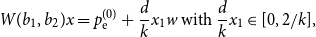 \begin{align*} W(b_1,b_2)x=p^{(0)}_{\mathrm {e}}+\frac {d}{k}x_1w\textrm { with }\frac {d}{k}x_1\in [0,2/k]\textrm {,} \end{align*}
hence the image of $\mathcal X$
under
$\mathcal X$
under $W(b_1,b_2)$
is a subset of
$W(b_1,b_2)$
is a subset of $\mathcal W$
. Conversely, for
$\mathcal W$
. Conversely, for $y\in [0,2/k]$
and
$y\in [0,2/k]$
and $x=\frac {k}{2}yx^{(2)}\in \mathcal X$
we have
$x=\frac {k}{2}yx^{(2)}\in \mathcal X$
we have $W(b_1,b_2)x=p^{(0)}_{\mathrm {e}}+yw$
, which shows that
$W(b_1,b_2)x=p^{(0)}_{\mathrm {e}}+yw$
, which shows that $\mathcal W$
is the image of
$\mathcal W$
is the image of $\mathcal X$
under
$\mathcal X$
under $W(b_1,b_2)$
. This also shows that
$W(b_1,b_2)$
. This also shows that $\mathcal X_p$
is the preimage of
$\mathcal X_p$
is the preimage of $p\in \mathcal W$
, since for
$p\in \mathcal W$
, since for $y\in [0,2/k]$
and
$y\in [0,2/k]$
and $p=p^{(0)}_{\mathrm {e}}+yw$
we have
$p=p^{(0)}_{\mathrm {e}}+yw$
we have $p(1,1)=y$
. This in turn directly yields that
$p(1,1)=y$
. This in turn directly yields that $\mathcal X_{p^{(s)}_{\mathrm {e}}}=\{p^{(s)}\}$
for
$\mathcal X_{p^{(s)}_{\mathrm {e}}}=\{p^{(s)}\}$
for $s\in \{0,2\}$
. To see that
$s\in \{0,2\}$
. To see that $\mathcal X_p$
contains interior points of
$\mathcal X_p$
contains interior points of $\mathcal X$
otherwise, we can consider non-trivial convex combinations of
$\mathcal X$
otherwise, we can consider non-trivial convex combinations of $x^*$
and
$x^*$
and $x^{(0)}$
for
$x^{(0)}$
for $\frac {k}{d}p(1,1)\lt x^*_1$
and non-trivial convex combinations of
$\frac {k}{d}p(1,1)\lt x^*_1$
and non-trivial convex combinations of $x^*$
and
$x^*$
and $x^{(2)}$
for
$x^{(2)}$
for $\frac {k}{d}p(1,1)\gt x^*_1$
, which are points in the interior of
$\frac {k}{d}p(1,1)\gt x^*_1$
, which are points in the interior of $\mathcal X$
.
$\mathcal X$
.
Notice that in the two-dimensional case at hand, the proof of Lemma 5.2 is overly formal. The set $\mathcal X$
is simply (the convex hull of) the triangle given by
$\mathcal X$
is simply (the convex hull of) the triangle given by $x^{(s)}$
,
$x^{(s)}$
, $s\in \{0,1,2\}$
, with
$s\in \{0,1,2\}$
, with $\mathcal X_p$
given by the vertical lines in
$\mathcal X_p$
given by the vertical lines in $\mathcal X$
with
$\mathcal X$
with $x_1=\frac {d}{k}p(1,1)$
. Further, the set
$x_1=\frac {d}{k}p(1,1)$
. Further, the set $\mathcal X_n$
is a canonical discretization of
$\mathcal X_n$
is a canonical discretization of $\mathcal X$
in that it is given by the points of the grid
$\mathcal X$
in that it is given by the points of the grid $(m^{-1}\mathbb {Z})^2$
contained in the triangle
$(m^{-1}\mathbb {Z})^2$
contained in the triangle $\mathcal X$
.
$\mathcal X$
.
5.4 Proof of Lemma 2.4
We derive Lemma 2.4 from the following stronger assertion.
Lemma 5.3.
Let $\mathcal U\subseteq \mathcal P(\{0,1,2\})$
be a subset with non-empty interior and such that the closure of
$\mathcal U\subseteq \mathcal P(\{0,1,2\})$
be a subset with non-empty interior and such that the closure of $\mathcal U$
is contained in the interior of
$\mathcal U$
is contained in the interior of $\mathcal P(\{0,1,2\})$
. Then there exists a constant
$\mathcal P(\{0,1,2\})$
. Then there exists a constant $c=c(\mathcal U)\in \mathbb {R}_{\gt 0}$
such that for all
$c=c(\mathcal U)\in \mathbb {R}_{\gt 0}$
such that for all $n\in \mathcal N$
and all
$n\in \mathcal N$
and all $p\in \mathcal P_n\cap \mathcal U$
we have
$p\in \mathcal P_n\cap \mathcal U$
we have $\tilde E(p)e^{-c/n}\le E(p)\le \tilde E(p)e^{c/n}$
, where
$\tilde E(p)e^{-c/n}\le E(p)\le \tilde E(p)e^{c/n}$
, where
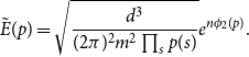 \begin{align*} \tilde E(p)=\sqrt {\frac {d^3}{(2\pi )^2m^2\prod _{s}p(s)}}e^{n\phi _2(p)}\textrm {.} \end{align*}
Proof. Let $\mathcal C$
denote the closure of
$\mathcal C$
denote the closure of $\mathcal U$
and
$\mathcal U$
and $\pi _s\,:\,\mathcal C\rightarrow [0,1]$
,
$\pi _s\,:\,\mathcal C\rightarrow [0,1]$
, $p\mapsto p(s)$
the projection for
$p\mapsto p(s)$
the projection for $s\in \{0,1,2\}$
. Since
$s\in \{0,1,2\}$
. Since $\mathcal C$
is compact, the continuous map
$\mathcal C$
is compact, the continuous map $\pi _s$
attains its maximum
$\pi _s$
attains its maximum $p_+(s)$
and its minimum
$p_+(s)$
and its minimum $p_-(s)$
, which directly gives
$p_-(s)$
, which directly gives $0\lt p_-(s)\lt p_+(s)\lt 1$
since all
$0\lt p_-(s)\lt p_+(s)\lt 1$
since all $p\in \mathcal C$
are fully supported and the interior of
$p\in \mathcal C$
are fully supported and the interior of $\mathcal C$
is non-empty (that gives the second inequality). Using Lemma 5.2, the continuous map
$\mathcal C$
is non-empty (that gives the second inequality). Using Lemma 5.2, the continuous map $\pi \,:\,\mathcal C\rightarrow [0,2/k]$
,
$\pi \,:\,\mathcal C\rightarrow [0,2/k]$
, $p\mapsto p_{\mathrm {e}}(1,1)$
, and the same reasoning as above we obtain the maximum
$p\mapsto p_{\mathrm {e}}(1,1)$
, and the same reasoning as above we obtain the maximum $p_{\mathrm {e},+}(1,1)$
and minimum
$p_{\mathrm {e},+}(1,1)$
and minimum $p_{\mathrm {e},-}(1,1)$
of
$p_{\mathrm {e},-}(1,1)$
of $\pi$
with
$\pi$
with $0\lt p_{\mathrm {e},-}(1,1)\lt p_{\mathrm {e},+}(1,1)\lt 2/k$
, which directly give the bounds
$0\lt p_{\mathrm {e},-}(1,1)\lt p_{\mathrm {e},+}(1,1)\lt 2/k$
, which directly give the bounds $p_{\mathrm {e},-}(x)$
,
$p_{\mathrm {e},-}(x)$
, $p_{\mathrm {e},+}(x)\gt 0$
for
$p_{\mathrm {e},+}(x)\gt 0$
for $x\in \{0,1\}^2$
as functions of
$x\in \{0,1\}^2$
as functions of $p_{\mathrm {e},+}(1,1)$
and
$p_{\mathrm {e},+}(1,1)$
and $p_{\mathrm {e},-}(1,1)$
. Now, we can use these bounds with the Stirling bound to obtain a constant
$p_{\mathrm {e},-}(1,1)$
. Now, we can use these bounds with the Stirling bound to obtain a constant $c\in \mathbb {R}_{\gt 0}$
such that for all
$c\in \mathbb {R}_{\gt 0}$
such that for all $n\in \mathcal N$
and
$n\in \mathcal N$
and $p\in \mathcal P_n\cap \mathcal C$
we have
$p\in \mathcal P_n\cap \mathcal C$
we have $E^{\prime}(p)e^{-c/n}\le E(p)\le E^{\prime}(p)e^{c/n}$
, where
$E^{\prime}(p)e^{-c/n}\le E(p)\le E^{\prime}(p)e^{c/n}$
, where
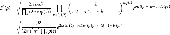 \begin{align*} E^{\prime}(p)&=\sqrt {\frac {2\pi md^3}{\prod _{s}(2\pi mp(s))}}\prod _{s\in \{0,1,2\}}\binom {k}{s,2-s,2-s,k-4+s}^{mp(s)} e^{mH(p)-(d-1)nH(p_{\mathrm {e}})}\\ &=\sqrt {\frac {d^3}{(2\pi )^2m^2\prod _{s}p(s)}}e^{2m\ln \binom {k}{2}-mD_{\textrm {KL}}(p\parallel p^*)-(d-1)nH(p_{\mathrm {e}})}\textrm {.} \end{align*}
To see that $E^{\prime}(p)=\tilde E(p)$
, we observe that
$E^{\prime}(p)=\tilde E(p)$
, we observe that $D_{\textrm {KL}}(p_{\mathrm {e}} \parallel p^*_{\mathrm {e}})=2H(2/k)-H(p_{\mathrm {e}})$
, since
$D_{\textrm {KL}}(p_{\mathrm {e}} \parallel p^*_{\mathrm {e}})=2H(2/k)-H(p_{\mathrm {e}})$
, since $H(p^*_{\mathrm {e}})=2H(2/k)$
,
$H(p^*_{\mathrm {e}})=2H(2/k)$
, $p_{\mathrm {e}}(1,0)=p_{\mathrm {e}}(0,1)$
, and
$p_{\mathrm {e}}(1,0)=p_{\mathrm {e}}(0,1)$
, and $p_{\mathrm {e}}(1,1)+p_{\mathrm {e}}(1,0)=2/k$
for any
$p_{\mathrm {e}}(1,1)+p_{\mathrm {e}}(1,0)=2/k$
for any $p\in \mathcal P(\{0,1,2\})$
.
$p\in \mathcal P(\{0,1,2\})$
.
Now, Lemma 2.4 is an immediate corollary. To see this, fix a fully supported overlap distribution $p\in \mathcal P(\{0,1,2\})$
and a sequence
$p\in \mathcal P(\{0,1,2\})$
and a sequence $(p_n)_{n\in \mathcal N}\subseteq \mathcal P_n$
converging to
$(p_n)_{n\in \mathcal N}\subseteq \mathcal P_n$
converging to $p$
, e.g.
$p$
, e.g. $p_n=\iota (m^{-1}\lfloor mx_1\rfloor, m^{-1}\lfloor mx_2\rfloor )$
with
$p_n=\iota (m^{-1}\lfloor mx_1\rfloor, m^{-1}\lfloor mx_2\rfloor )$
with $\iota (x)=p$
and
$\iota (x)=p$
and $n$
sufficiently large. Further, fix a neighbourhood
$n$
sufficiently large. Further, fix a neighbourhood $\mathcal U$
of
$\mathcal U$
of $p$
as described in Lemma 5.3, which is possible since
$p$
as described in Lemma 5.3, which is possible since $p$
is fully supported. Then we have
$p$
is fully supported. Then we have $p_n\in \mathcal U$
for sufficiently large
$p_n\in \mathcal U$
for sufficiently large $n$
, hence with the continuity of
$n$
, hence with the continuity of $\phi _2$
we have
$\phi _2$
we have
 \begin{align*} \lim _{n\rightarrow \infty }\frac {1}{n}\ln (E(p_n)) =\lim _{n\rightarrow \infty }\frac {1}{n}\ln (\tilde E(p_n)) =\lim _{n\rightarrow \infty }\phi _2(p_n)=\phi _2(p)\textrm {.} \end{align*}
5.5 Proof of Proposition 2.6
We postpone the proof of Proposition 2.5 and continue with Laplace’s method for sums using the result. We obtain that
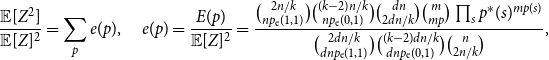 \begin{align*} \frac {\mathbb {E}[Z^2]}{\mathbb {E}[Z]^2}=\sum _pe(p)\textrm {, } \quad e(p)=\frac {E(p)}{\mathbb {E}[Z]^2} =\frac {\binom {2n/k}{np_{\mathrm {e}}(1,1)}\binom {(k-2)n/k}{np_{\mathrm {e}}(0,1)}\binom {dn}{2dn/k}\binom {m}{mp}\prod _sp^*(s)^{mp(s)}} {\binom {2dn/k}{dnp_{\mathrm {e}}(1,1)}\binom {(k-2)dn/k}{dnp_{\mathrm {e}}(0,1)}\binom {n}{2n/k}}\textrm {,} \end{align*}
where the sum is over $p\in \mathcal P_n$
. First, we use Proposition 2.5 to show that Laplace’s method of sums is applicable. While we have already established that
$p\in \mathcal P_n$
. First, we use Proposition 2.5 to show that Laplace’s method of sums is applicable. While we have already established that $\Delta _{d^*}$
is non-negative, we still need to ensure that
$\Delta _{d^*}$
is non-negative, we still need to ensure that $p^*$
is the unique minimizer of
$p^*$
is the unique minimizer of $\Delta _d$
for
$\Delta _d$
for $d\lt d^*$
and that the Hessian at
$d\lt d^*$
and that the Hessian at $p^*$
is positive definite. We will need the second order Taylor approximation of the KL divergence. To be specific, let
$p^*$
is positive definite. We will need the second order Taylor approximation of the KL divergence. To be specific, let $\mu ^*$
have finite non-trivial support
$\mu ^*$
have finite non-trivial support $\mathcal S$
and let
$\mathcal S$
and let $f\,:\,\mathcal P(\mathcal S)\rightarrow \mathbb {R}_{\ge 0}$
,
$f\,:\,\mathcal P(\mathcal S)\rightarrow \mathbb {R}_{\ge 0}$
, $\mu \mapsto D_{\textrm {KL}}(\mu \parallel \mu ^*)$
, be the corresponding KL divergence. Then
$\mu \mapsto D_{\textrm {KL}}(\mu \parallel \mu ^*)$
, be the corresponding KL divergence. Then
 \begin{align*} f^{(2)}\,:\,\mathcal P(\mathcal S)\rightarrow \mathbb {R}_{\ge 0},\quad \mu \mapsto \frac {1}{2}D_{\chi ^2}(\mu \parallel \mu ^*) =\frac 12\sum _s\frac {(\mu (s)-\mu ^*(s))^2}{\mu ^*(s)} =\frac 12(\mu -\mu ^*)^{\mathrm {t}}D_{\mu ^*}^{-1}(\mu -\mu ^*)\textrm {, } \end{align*}
is the second order Taylor approximation of $f$
at
$f$
at $\mu ^*$
, where
$\mu ^*$
, where $D_{\chi ^2}(\mu \parallel \mu ^*)$
denotes Pearson’s
$D_{\chi ^2}(\mu \parallel \mu ^*)$
denotes Pearson’s $\chi ^2$
divergence,
$\chi ^2$
divergence, $D_{\mu ^*}=(\delta _{i,j}\mu ^*(i))_{i,j\in \mathcal S}$
the matrix with
$D_{\mu ^*}=(\delta _{i,j}\mu ^*(i))_{i,j\in \mathcal S}$
the matrix with $\mu ^*$
on the diagonal, and
$\mu ^*$
on the diagonal, and $\delta _{i,j}=1$
if
$\delta _{i,j}=1$
if $i=j$
and
$i=j$
and $0$
otherwise; this can be easily seen by considering the extension of
$0$
otherwise; this can be easily seen by considering the extension of $f$
to
$f$
to $\mathbb {R}_{\ge 0}^{\mathcal S}$
. On the other hand, we would like to consider
$\mathbb {R}_{\ge 0}^{\mathcal S}$
. On the other hand, we would like to consider $\Delta _d$
as a function over the suitable domain
$\Delta _d$
as a function over the suitable domain $\mathcal X$
from Section 5.3, however relative to the base point
$\mathcal X$
from Section 5.3, however relative to the base point $p^*$
. Hence, let
$p^*$
. Hence, let $\mathcal X^*=\{x-x^*:x\in \mathcal X\}$
be the triangle
$\mathcal X^*=\{x-x^*:x\in \mathcal X\}$
be the triangle $\mathcal X$
centred at
$\mathcal X$
centred at $x^*$
instead of
$x^*$
instead of $x^{(0)}$
, and
$x^{(0)}$
, and $\iota ^*\,:\,\mathcal X^*\rightarrow \mathcal P(\{0,1,2\})$
the bijection given by
$\iota ^*\,:\,\mathcal X^*\rightarrow \mathcal P(\{0,1,2\})$
the bijection given by
 \begin{align*} \iota ^*(x)=\iota (x+x^*)=p^{(0)}+(b_1,b_2)x+(b_1,b_2)x^*=\iota (x^*)+(b_1,b_2)x=p^*+(b_1,b_2)x \end{align*}
for $x\in \mathcal X^*$
, with
$x\in \mathcal X^*$
, with $b_1,b_2$
from Equation (4). Now, let
$b_1,b_2$
from Equation (4). Now, let $\gamma _d\,:\,\mathcal X^*\rightarrow \mathbb {R}_{\ge 0}$
,
$\gamma _d\,:\,\mathcal X^*\rightarrow \mathbb {R}_{\ge 0}$
, $x\mapsto \Delta _d(\iota ^*(x))$
, denote the corresponding parametrization of
$x\mapsto \Delta _d(\iota ^*(x))$
, denote the corresponding parametrization of $\Delta _d$
. Then, using the chain rule for multivariate calculus as indicated above for both
$\Delta _d$
. Then, using the chain rule for multivariate calculus as indicated above for both $(b_1,b_2)$
and
$(b_1,b_2)$
and $W$
from (3), we derive the Hessian
$W$
from (3), we derive the Hessian
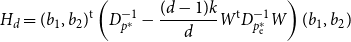 \begin{align} H_d=(b_1,b_2)^{\mathrm {t}}\left (D_{p^*}^{-1}-\frac {(d-1)k}{d}W^{\mathrm {t}}D_{p^*_{\mathrm {e}}}^{-1}W\right )(b_1,b_2) \end{align}
of $\gamma _d$
at
$\gamma _d$
at $0_{[2]}\in \mathbb {R}^2$
, using the shorthand
$0_{[2]}\in \mathbb {R}^2$
, using the shorthand $D_{\mu ^*}=(\delta _{i,j}\mu ^*(i))_{i,j}$
. The properties of the KL divergence imply that
$D_{\mu ^*}=(\delta _{i,j}\mu ^*(i))_{i,j}$
. The properties of the KL divergence imply that $\gamma _d(0_{[2]})=0$
and
$\gamma _d(0_{[2]})=0$
and $\gamma _d$
has a stationary point at
$\gamma _d$
has a stationary point at $0_{[2]}$
. Now, the second order Taylor approximation
$0_{[2]}$
. Now, the second order Taylor approximation $\gamma ^{(2)}_d\,:\,\mathcal X^*\rightarrow \mathbb {R}$
,
$\gamma ^{(2)}_d\,:\,\mathcal X^*\rightarrow \mathbb {R}$
, $x\mapsto \frac {1}{2}x^{\mathrm {t}}H_dx$
, of
$x\mapsto \frac {1}{2}x^{\mathrm {t}}H_dx$
, of $\gamma _d$
at
$\gamma _d$
at $0_{[2]}$
can be written as
$0_{[2]}$
can be written as $\gamma ^{(2)}_d=\Delta ^{(2)}_d\circ \iota ^*$
with
$\gamma ^{(2)}_d=\Delta ^{(2)}_d\circ \iota ^*$
with
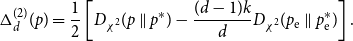 \begin{align} \Delta ^{(2)}_d(p)&=\frac {1}{2}\left [D_{\chi ^2}(p\parallel p^*)-\frac {(d-1)k}{d}D_{\chi ^2}(p_{\mathrm {e}}\parallel p^*_{\mathrm {e}})\right ]. \end{align}
Further, for any neighbourhood $\mathcal U$
of
$\mathcal U$
of $0_{[2]}$
such that the closure of
$0_{[2]}$
such that the closure of $\mathcal U$
is contained in the interior of
$\mathcal U$
is contained in the interior of $\mathcal X^*$
, Taylor’s theorem yields a constant
$\mathcal X^*$
, Taylor’s theorem yields a constant $c\in \mathbb {R}_{\gt 0}$
such that
$c\in \mathbb {R}_{\gt 0}$
such that
 \begin{align} \gamma ^{(2)}_d(x)-c\|x\|_2^3\le \gamma _d(x)\le \gamma ^{(2)}_d(x)+c\|x\|_2^3 \end{align}
for all $x\in \mathcal U$
. Since
$x\in \mathcal U$
. Since $H_d$
is symmetric, let
$H_d$
is symmetric, let $\lambda _1$
,
$\lambda _1$
, $\lambda _2\in \mathbb {R}$
with
$\lambda _2\in \mathbb {R}$
with $\lambda _1\le \lambda _2$
denote its eigenvalues and fix a corresponding orthonormal basis of eigenvectors
$\lambda _1\le \lambda _2$
denote its eigenvalues and fix a corresponding orthonormal basis of eigenvectors $v_1$
,
$v_1$
, $v_2\in \mathbb {R}^2$
, i.e.
$v_2\in \mathbb {R}^2$
, i.e. $H_dv_1=\lambda _1v_1$
and
$H_dv_1=\lambda _1v_1$
and $H_dv_2=\lambda _2v_2$
.
$H_dv_2=\lambda _2v_2$
.
Formally and analogously to the KL divergence we will take the liberty to identify $\Delta _d$
and
$\Delta _d$
and $\Delta ^{(2)}_d$
with their extensions to the maximal domains
$\Delta ^{(2)}_d$
with their extensions to the maximal domains $\mathcal D\subseteq \mathbb {R}^{\{0,1,2\}}$
and
$\mathcal D\subseteq \mathbb {R}^{\{0,1,2\}}$
and $\mathcal D^{(2)}=\mathbb {R}^{\{0,1,2\}}$
respectively. In particular, Lemma 5.2 shows that for any fully supported
$\mathcal D^{(2)}=\mathbb {R}^{\{0,1,2\}}$
respectively. In particular, Lemma 5.2 shows that for any fully supported $p\in \mathcal P(\{0,1,2\})$
the edge distribution
$p\in \mathcal P(\{0,1,2\})$
the edge distribution $p_{\mathrm {e}}$
also has full support, hence we can use the Lipschitz continuity of
$p_{\mathrm {e}}$
also has full support, hence we can use the Lipschitz continuity of $W$
on
$W$
on $\mathbb {R}^{\{0,1,2\}}$
to find
$\mathbb {R}^{\{0,1,2\}}$
to find $\varepsilon \in \mathbb {R}_{\gt 0}$
such that both
$\varepsilon \in \mathbb {R}_{\gt 0}$
such that both $p^{\prime}\gt 0$
and
$p^{\prime}\gt 0$
and $Wp^{\prime}\gt 0$
for any
$Wp^{\prime}\gt 0$
for any $p^{\prime}\in \mathcal B_\varepsilon (p)\subseteq \mathbb {R}_{\gt 0}^{\{0,1,2\}}$
and thereby
$p^{\prime}\in \mathcal B_\varepsilon (p)\subseteq \mathbb {R}_{\gt 0}^{\{0,1,2\}}$
and thereby $\Delta _d$
is well-defined and smooth on
$\Delta _d$
is well-defined and smooth on $\mathcal B_\varepsilon (p)$
.
$\mathcal B_\varepsilon (p)$
.
Lemma 5.4.
Let $k\in \mathbb {Z}_{\ge 4}$
and
$k\in \mathbb {Z}_{\ge 4}$
and $d\in (0,d^*)$
. Then the unique minimizer of
$d\in (0,d^*)$
. Then the unique minimizer of $\gamma _d$
is
$\gamma _d$
is $0_{[2]}$
and
$0_{[2]}$
and $H_d$
is positive definite.
$H_d$
is positive definite.
Proof. Using Proposition 2.5 we know that $H_{d^*}$
is positive semidefinite since
$H_{d^*}$
is positive semidefinite since $0_{[2]}$
is a global minimum of
$0_{[2]}$
is a global minimum of $\gamma _{d^*}$
. This in turn yields that
$\gamma _{d^*}$
. This in turn yields that $\gamma ^{(2)}_{d^*}\ge 0$
or equivalently
$\gamma ^{(2)}_{d^*}\ge 0$
or equivalently $\Delta ^{(2)}_{d^*}\ge 0$
. Now, for any
$\Delta ^{(2)}_{d^*}\ge 0$
. Now, for any $d\lt d^*$
the unique minimizer of
$d\lt d^*$
the unique minimizer of $\Delta _d$
is
$\Delta _d$
is $p^*$
since
$p^*$
since $\Delta _d(p^*)=0$
, further
$\Delta _d(p^*)=0$
, further $\Delta _d(p)\gt 0$
for any
$\Delta _d(p)\gt 0$
for any $p\neq p^*$
with
$p\neq p^*$
with $p_{\mathrm {e}}=p^*_{\mathrm {e}}$
and
$p_{\mathrm {e}}=p^*_{\mathrm {e}}$
and
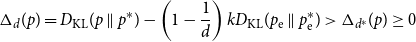 \begin{align*} \Delta _d(p)=D_{\textrm {KL}}(p\parallel p^*)-\left (1-\frac {1}{d}\right )kD_{\textrm {KL}}(p_{\mathrm {e}}\parallel p^*_{\mathrm {e}}) \gt \Delta _{d^*}(p)\ge 0 \end{align*}
for any $p$
with
$p$
with $p_{\mathrm {e}}\neq p^*_{\mathrm {e}}$
. But the same argumentation shows that
$p_{\mathrm {e}}\neq p^*_{\mathrm {e}}$
. But the same argumentation shows that $p^*$
is the unique minimizer of
$p^*$
is the unique minimizer of $\Delta ^{(2)}_d$
, since
$\Delta ^{(2)}_d$
, since $D_{\chi ^2}(\mu \parallel \mu ^*)$
is also minimal with value
$D_{\chi ^2}(\mu \parallel \mu ^*)$
is also minimal with value $0$
iff
$0$
iff $\mu =\mu ^*$
. This in turn shows that
$\mu =\mu ^*$
. This in turn shows that $\gamma ^{(2)}_d$
is uniquely minimized at
$\gamma ^{(2)}_d$
is uniquely minimized at $0_{[2]}$
and hence
$0_{[2]}$
and hence $H_d$
is positive definite.
$H_d$
is positive definite.
Let $\eta _{\mathrm {KL}}=\sup _{p\neq p^*}\frac {D_{\textrm {KL}}(p_{\mathrm {e}}\parallel p^*_{\mathrm {e}})}{D_{\textrm {KL}}(p\parallel p^*)}$
denote the contraction coefficient with respect to the KL divergence. Notice that by Proposition 2.5 we have
$\eta _{\mathrm {KL}}=\sup _{p\neq p^*}\frac {D_{\textrm {KL}}(p_{\mathrm {e}}\parallel p^*_{\mathrm {e}})}{D_{\textrm {KL}}(p\parallel p^*)}$
denote the contraction coefficient with respect to the KL divergence. Notice that by Proposition 2.5 we have $\frac {d^*}{(d^*-1)k}\ge \frac {D_{\textrm {KL}}(p_{\mathrm {e}}\parallel p^*_{\mathrm {e}})}{D_{\textrm {KL}}(p\parallel p^*)}$
for all
$\frac {d^*}{(d^*-1)k}\ge \frac {D_{\textrm {KL}}(p_{\mathrm {e}}\parallel p^*_{\mathrm {e}})}{D_{\textrm {KL}}(p\parallel p^*)}$
for all $p\neq p^*$
with equality for
$p\neq p^*$
with equality for $p=p^{(2)}$
, hence
$p=p^{(2)}$
, hence $\eta _{\mathrm {KL}}=\frac {d^*}{(d^*-1)k}$
(so Proposition 2.5 indeed confirms the conjecture by the authors in [Reference Panagiotou and Pasch36]). Further, let
$\eta _{\mathrm {KL}}=\frac {d^*}{(d^*-1)k}$
(so Proposition 2.5 indeed confirms the conjecture by the authors in [Reference Panagiotou and Pasch36]). Further, let $\eta _{\chi ^2}=\sup _{p\neq p^*}\frac {D_{\chi ^2}(p_{\mathrm {e}}\parallel p^*_{\mathrm {e}})}{D_{\chi ^2}(p\parallel p^*)}$
denote the contraction coefficient with respect to the
$\eta _{\chi ^2}=\sup _{p\neq p^*}\frac {D_{\chi ^2}(p_{\mathrm {e}}\parallel p^*_{\mathrm {e}})}{D_{\chi ^2}(p\parallel p^*)}$
denote the contraction coefficient with respect to the $\chi ^2$
divergence. The proof of Lemma 5.4 suggests that
$\chi ^2$
divergence. The proof of Lemma 5.4 suggests that $\eta _{\chi ^2}\le \eta _{\mathrm {KL}}$
, a result known from the literature.
$\eta _{\chi ^2}\le \eta _{\mathrm {KL}}$
, a result known from the literature.
In the rest of this section we discuss the straightforward (but cumbersome) application of Laplace’s method for sums. For convenience, we first show that the boundaries can be neglected and derive the asymptotics of the sum on the interior using the uniform convergence established in Lemma 5.3.
Lemma 5.5.
Let $d\in (0,d^*)$
and let
$d\in (0,d^*)$
and let $\mathcal U$
be a neighbourhood of
$\mathcal U$
be a neighbourhood of $p^*$
such that its closure is contained in the interior of
$p^*$
such that its closure is contained in the interior of $\mathcal P(\{0,1,2\})$
. Then
$\mathcal P(\{0,1,2\})$
. Then
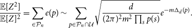 \begin{align*} \frac {\mathbb {E}[Z^2]}{\mathbb {E}[Z]^2}=\sum _{\in \mathcal P_n}e(p)\sim \sum _{p\in \mathcal P_n\cap \mathcal U}\sqrt {\frac {d}{(2\pi )^2m^2\prod _sp(s)}}e^{-m\Delta _d(p)}\textrm {.} \end{align*}
Proof. Let $\Delta _{\min }\gt 0$
denote the global minimum of
$\Delta _{\min }\gt 0$
denote the global minimum of $\Delta _d$
on
$\Delta _d$
on $\mathcal P(\{0,1,2\})\setminus \mathcal U$
. Now, we can use the well-known bounds
$\mathcal P(\{0,1,2\})\setminus \mathcal U$
. Now, we can use the well-known bounds $\frac {1}{a+1}\exp (aH(\frac {b}{a}))\le \binom {a}{b}\le \exp (aH(\frac {b}{a}))$
for binomial coefficients and the corresponding upper bound for multinomial coefficients (using the entropy of the distribution determined by the weights
$\frac {1}{a+1}\exp (aH(\frac {b}{a}))\le \binom {a}{b}\le \exp (aH(\frac {b}{a}))$
for binomial coefficients and the corresponding upper bound for multinomial coefficients (using the entropy of the distribution determined by the weights $\frac {b_i}{a}$
) to derive
$\frac {b_i}{a}$
) to derive
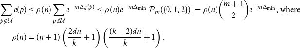 \begin{align*} \sum _{p\not \in \mathcal U}e(p) &\le \rho (n)\sum _{p\not \in \mathcal U}e^{-m\Delta _d(p)} \le \rho (n)e^{-m\Delta _{\min }}|\mathcal P_m(\{0,1,2\})| = \rho (n)\binom {m+1}{2}e^{-m\Delta _{\min }}\textrm {, where}\\ \rho (n)&=(n+1)\left (\frac {2dn}{k}+1\right )\left (\frac {(k-2)dn}{k}+1\right )\textrm {.} \end{align*}
Here, we used the form of $e(p)$
introduced at the beginning of this section and further notice that the bounds used are tight for the log-densities, i.e. the exponent is
$e(p)$
introduced at the beginning of this section and further notice that the bounds used are tight for the log-densities, i.e. the exponent is $\Delta _d(p)$
by the computations in Section 5.4. The right-hand side vanishes for
$\Delta _d(p)$
by the computations in Section 5.4. The right-hand side vanishes for $n$
tending to infinity, hence we have
$n$
tending to infinity, hence we have
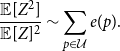 \begin{align*} \frac {\mathbb {E}[Z^2]}{\mathbb {E}[Z]^2}\sim \sum _{p\in \mathcal U}e(p)\textrm {.} \end{align*}
Now, the result directly follows using Lemma 5.3 and Lemma 2.2.
Lemma 5.5 shows that the overlap distributions $p$
with material contributions
$p$
with material contributions $e(p)$
to the second moment are concentrated around
$e(p)$
to the second moment are concentrated around $p^*$
. Hence, instead of considering a fixed neighbourhood
$p^*$
. Hence, instead of considering a fixed neighbourhood $\mathcal U$
of
$\mathcal U$
of $p^*$
we consider a sequence
$p^*$
we consider a sequence $(\mathcal U_n)_{n\in \mathcal N}$
of decreasing neighbourhoods. First, we choose a scaling that improves the assertion of Lemma 5.5 and further allows to simplify the asymptotics of the right-hand side, in the sense that the leading factor collapses to a constant and
$(\mathcal U_n)_{n\in \mathcal N}$
of decreasing neighbourhoods. First, we choose a scaling that improves the assertion of Lemma 5.5 and further allows to simplify the asymptotics of the right-hand side, in the sense that the leading factor collapses to a constant and $\gamma _d(x)=\Delta _d(\iota ^*(x))$
can be replaced by its second order Taylor approximation
$\gamma _d(x)=\Delta _d(\iota ^*(x))$
can be replaced by its second order Taylor approximation $\gamma ^{(2)}_d(x)=\Delta ^{(2)}_d(\iota ^*(x))=\frac {1}{2}x^{\mathrm {t}}H_dx$
from above (7). For this purpose let
$\gamma ^{(2)}_d(x)=\Delta ^{(2)}_d(\iota ^*(x))=\frac {1}{2}x^{\mathrm {t}}H_dx$
from above (7). For this purpose let $\mathcal U^*\subseteq \mathcal X^*$
be a sufficiently small neighbourhood of
$\mathcal U^*\subseteq \mathcal X^*$
be a sufficiently small neighbourhood of $0_{[2]}$
(in particular bounded away from the boundary of
$0_{[2]}$
(in particular bounded away from the boundary of $\mathcal X^*$
), further
$\mathcal X^*$
), further
 \begin{align*} \mathcal U^*_n=\left \{x\in \mathcal X^*\,:\, \|x\|_2\lt \frac {\ln (m)}{\sqrt {m}}\right \}\textrm { and } \mathcal X^*_n=\left \{x-x^*\,:\,x\in \mathcal X_n\right \}\cap \mathcal U^*_n \textrm { for }n\in \mathcal N\textrm {.} \end{align*}
In the following we restrict to $n\ge n_0$
where
$n\ge n_0$
where $n_0\in \mathcal N$
is such that
$n_0\in \mathcal N$
is such that $\mathcal U^*_{n_0}\subseteq \mathcal U^*$
.
$\mathcal U^*_{n_0}\subseteq \mathcal U^*$
.
Lemma 5.6.
For $d\in (0,d^*)$
we have
$d\in (0,d^*)$
we have
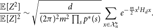 \begin{align*} \frac {\mathbb {E}[Z^2]}{\mathbb {E}[Z]^2} \sim \sqrt {\frac {d}{(2\pi )^2m^2\prod _sp^*(s)}}\sum _{x\in \mathcal X^*_n}e^{-\frac {m}{2}x^{\mathrm {t}}H_dx}\textrm {.} \end{align*}
Proof. First, notice that we can apply Lemma 5.5 to $\iota ^*(\mathcal U^*)$
. So, we need to show that the sum over
$\iota ^*(\mathcal U^*)$
. So, we need to show that the sum over $\mathcal U^*\setminus \mathcal U^*_n$
is negligible. Then we proceed to derive the asymptotics of the sum over
$\mathcal U^*\setminus \mathcal U^*_n$
is negligible. Then we proceed to derive the asymptotics of the sum over $\mathcal U^*_n$
. Obviously, we have
$\mathcal U^*_n$
. Obviously, we have $\gamma _{\min }(n)\rightarrow 0$
for
$\gamma _{\min }(n)\rightarrow 0$
for $n\rightarrow \infty$
with
$n\rightarrow \infty$
with $\gamma _{\min }(n)=\min _{x\not \in \mathcal U^*_n}\gamma _d(x)\gt 0$
, since
$\gamma _{\min }(n)=\min _{x\not \in \mathcal U^*_n}\gamma _d(x)\gt 0$
, since $\gamma _d(x)=\Delta _d(\iota ^*(x))$
is continuous and
$\gamma _d(x)=\Delta _d(\iota ^*(x))$
is continuous and $\gamma _d(0_{[2]})=0$
. The main objective of the proof is to show that
$\gamma _d(0_{[2]})=0$
. The main objective of the proof is to show that $\gamma _{\min }(n)$
converges to zero sufficiently slow. But with
$\gamma _{\min }(n)$
converges to zero sufficiently slow. But with $\gamma ^{(2)}_d(x)=\frac {1}{2}x^{\mathrm {t}}H_dx$
from above (7) and for any
$\gamma ^{(2)}_d(x)=\frac {1}{2}x^{\mathrm {t}}H_dx$
from above (7) and for any $x\in \mathbb {R}^2$
we have
$x\in \mathbb {R}^2$
we have
 \begin{align*} \gamma ^{(2)}_d((v_1,v_2)x)&=\frac {1}{2}(\lambda _1x_1^2+\lambda _2x_2^2) \ge \frac {\lambda _1}{2}\|x\|_2^2=\frac {\lambda _1}{2}\|(v_1,v_2)x\|_2^2 \end{align*}
since $(v_1,v_2)$
is an orthonormal basis, so
$(v_1,v_2)$
is an orthonormal basis, so $\gamma ^{(2)}_d(x)\ge \frac {\lambda _1}{2}\|x\|_2^2$
for all
$\gamma ^{(2)}_d(x)\ge \frac {\lambda _1}{2}\|x\|_2^2$
for all $x\in \mathbb {R}^2$
. Now, for any sufficiently small
$x\in \mathbb {R}^2$
. Now, for any sufficiently small $\varepsilon \in (0,1)$
let
$\varepsilon \in (0,1)$
let $c\in \mathbb {R}_{\gt 0}$
be the constant for
$c\in \mathbb {R}_{\gt 0}$
be the constant for $\mathcal B_{\varepsilon }(0_{[2]})$
from Taylor’s theorem applied to
$\mathcal B_{\varepsilon }(0_{[2]})$
from Taylor’s theorem applied to $\gamma _d$
at
$\gamma _d$
at $0_{[2]}$
, then for any
$0_{[2]}$
, then for any $x\in \mathcal U^*=\mathcal B_{\varepsilon }(0_{[2]})\cap \mathcal B_\delta (0_{[2]})$
, with
$x\in \mathcal U^*=\mathcal B_{\varepsilon }(0_{[2]})\cap \mathcal B_\delta (0_{[2]})$
, with $\delta =\frac {\varepsilon \lambda _1}{2c}$
, we have
$\delta =\frac {\varepsilon \lambda _1}{2c}$
, we have $\gamma _d(x)\ge (1-\varepsilon )\gamma ^{(2)}_d(x)$
since
$\gamma _d(x)\ge (1-\varepsilon )\gamma ^{(2)}_d(x)$
since
 \begin{align*} \gamma _d(x)-(1-\varepsilon )\gamma ^{(2)}_d(x)\ge \varepsilon \gamma ^{(2)}_d(x)-c\|x\|_2^3 \ge \left (\frac {\varepsilon \lambda _1}{2}-c\delta \right )\|x\|_2^2=0\textrm {.} \end{align*}
In combination we have $\gamma _d(x)\ge \frac {(1-\varepsilon )\lambda _1}{2}\|x\|_2^2$
and using
$\gamma _d(x)\ge \frac {(1-\varepsilon )\lambda _1}{2}\|x\|_2^2$
and using $p=\iota ^*(x)$
hence
$p=\iota ^*(x)$
hence
 \begin{align*} \lim _{n\rightarrow \infty }\sum _{x\not \in \mathcal U^*_n}e(p) &=\lim _{n\rightarrow \infty }\sum _{x\in \mathcal U^*\setminus \mathcal U^*_n}\sqrt {\frac {d}{(2\pi )^2m^2\prod _sp(s)}}e^{-m\gamma _d(x)} \le \lim _{n\rightarrow \infty }Cme^{-\frac {(1-\varepsilon )\lambda _1}{2}\ln (m)^2} =0\textrm {,} \end{align*}
by using (the proof of) Lemma 5.5 and some sufficiently large constant $C$
. With this we have
$C$
. With this we have
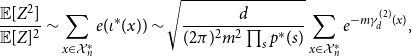 \begin{align*} \frac {\mathbb {E}[Z^2]}{\mathbb {E}[Z]^2} \sim \sum _{x\in \mathcal X^*_n}e(\iota ^*(x)) \sim \sqrt {\frac {d}{(2\pi )^2m^2\prod _sp^*(s)}}\sum _{x\in \mathcal X^*_n}e^{-m\gamma ^{(2)}_d(x)}\textrm {,} \end{align*}
where the last equivalence follows from the fact that the leading factor converges to the respective constant uniformly on $\mathcal U^*_n$
and by (8) on
$\mathcal U^*_n$
and by (8) on $\mathcal U^*$
.
$\mathcal U^*$
.
Lemma 5.6 completes the analytical part of the proof. For the last, measure theoretic, part we recall the bijection $\iota _n$
from Lemma 5.1. The translation of the sum on the right-hand side of Lemma 5.6 into a Riemann sum and further into the integral
$\iota _n$
from Lemma 5.1. The translation of the sum on the right-hand side of Lemma 5.6 into a Riemann sum and further into the integral $\int g_\infty (x)\mathrm {d}x$
, where
$\int g_\infty (x)\mathrm {d}x$
, where
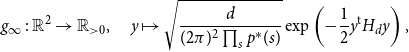 \begin{align*} g_{\infty }\,:\,\mathbb {R}^2\rightarrow \mathbb {R}_{\gt 0},\quad y \mapsto \sqrt {\frac {d}{(2\pi )^2\prod _sp^*(s)}}\exp \left ({-}\frac {1}{2}y^{\mathrm {t}}H_dy\right )\textrm {, } \end{align*}
is essentially given by the grid $\mathcal X_n\subseteq (m^{-1}\mathbb {Z})^2\subseteq \mathbb {R}^2$
. We make this rigorous in the following.
$\mathcal X_n\subseteq (m^{-1}\mathbb {Z})^2\subseteq \mathbb {R}^2$
. We make this rigorous in the following.
Lemma 5.7. We have
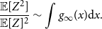 \begin{align*} \frac {\mathbb {E}[Z^2]}{\mathbb {E}[Z]^2} \sim \int g_\infty (x)\mathrm {d}x\textrm {.} \end{align*}
Proof. We start with the partition of $\mathbb {R}^2$
into the squares
$\mathbb {R}^2$
into the squares
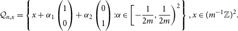 \begin{align*} \mathcal Q_{n,x}=\left \{x+\alpha _1\begin{pmatrix}1\\ 0\end{pmatrix}+\alpha _2\begin{pmatrix}0\\ 1\end{pmatrix}:\alpha \in \left [-\frac {1}{2m},\frac {1}{2m}\right )^2\right \}\textrm {, }x\in (m^{-1}\mathbb {Z})^2\textrm {.} \end{align*}
Next, we need a suitable selection of squares to cover the disc
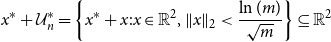 \begin{align*} x^*+\mathcal U^*_n=\left \{x^*+x:x\in \mathbb {R}^2,\|x\|_2\lt \frac {\ln (m)}{\sqrt {m}}\right \}\subseteq \mathbb {R}^2 \end{align*}
corresponding to the disc $\mathcal U^*_n$
. For this purpose let
$\mathcal U^*_n$
. For this purpose let $x_{\min }$
,
$x_{\min }$
, $x_{\max }\in (m^{-1}\mathbb {Z})^2$
be given by
$x_{\max }\in (m^{-1}\mathbb {Z})^2$
be given by
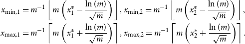 \begin{align*} x_{\min, 1}&=m^{-1}\left \lfloor m\left (x^*_1-\frac {\ln (m)}{\sqrt {m}}\right )\right \rfloor \textrm {, } x_{\min, 2}=m^{-1}\left \lfloor m\left (x^*_2-\frac {\ln (m)}{\sqrt {m}}\right )\right \rfloor \textrm {, }\\ x_{\max, 1}&=m^{-1}\left \lceil m\left (x^*_1+\frac {\ln (m)}{\sqrt {m}}\right )\right \rceil \textrm {, } x_{\max, 2}=m^{-1}\left \lceil m\left (x^*_2+\frac {\ln (m)}{\sqrt {m}}\right )\right \rceil \textrm {.} \end{align*}
Further, let $\mathcal{G}_n=(m^{-1}\mathbb {Z})^2\cap \left ([x_{\min, 1},x_{\max, 1}]\times [x_{\min, 2},x_{\max, 2}]\right )$
. By the definition of
$\mathcal{G}_n=(m^{-1}\mathbb {Z})^2\cap \left ([x_{\min, 1},x_{\max, 1}]\times [x_{\min, 2},x_{\max, 2}]\right )$
. By the definition of $x_{\min }$
and
$x_{\min }$
and $x_{\max }$
the points on the boundary are not in
$x_{\max }$
the points on the boundary are not in $x^*+\mathcal U^*_n$
, which ensures that
$x^*+\mathcal U^*_n$
, which ensures that $x^*+\mathcal U^*_n\subseteq \mathcal Q_n$
with
$x^*+\mathcal U^*_n\subseteq \mathcal Q_n$
with $\mathcal Q_n=\bigcup _{x\in \mathcal{G}_n}\mathcal Q_{n,x}$
. Further, we have
$\mathcal Q_n=\bigcup _{x\in \mathcal{G}_n}\mathcal Q_{n,x}$
. Further, we have $\mathcal Q_-\subseteq \mathcal Q_n\subseteq \mathcal Q_+$
with
$\mathcal Q_-\subseteq \mathcal Q_n\subseteq \mathcal Q_+$
with
 \begin{align*} \mathcal Q_-=\left \{x\in \mathbb {R}^2:\|x-x^*\|_{\infty }\le \frac {\ln (m)}{\sqrt {m}}\right \} \textrm {, } \mathcal Q_+=\left \{x\in \mathbb {R}^2:\|x-x^*\|_{\infty }\le \frac {\ln (m)}{\sqrt {m}}+\frac {3}{2m}\right \}\textrm {,} \end{align*}
which ensures that $\mathcal Q_n\subseteq \mathcal X$
for
$\mathcal Q_n\subseteq \mathcal X$
for $n\in \mathcal N$
sufficiently large. Now, we translate the notions back to
$n\in \mathcal N$
sufficiently large. Now, we translate the notions back to $\mathcal X^*$
using the bijection
$\mathcal X^*$
using the bijection $\tau \,:\,\mathbb {R}^2\rightarrow \mathbb {R}^2$
,
$\tau \,:\,\mathbb {R}^2\rightarrow \mathbb {R}^2$
, $x\mapsto x-x^*$
, i.e. let
$x\mapsto x-x^*$
, i.e. let $\mathcal{G}^*_n=\tau (\mathcal{G}_n)$
,
$\mathcal{G}^*_n=\tau (\mathcal{G}_n)$
, $\mathcal Q^*_{n,x}=\tau (\mathcal Q_{n,\tau ^{-1}(x)})$
for
$\mathcal Q^*_{n,x}=\tau (\mathcal Q_{n,\tau ^{-1}(x)})$
for $x\in \mathcal{G}^*_n$
,
$x\in \mathcal{G}^*_n$
, $\mathcal Q^*_n=\tau (\mathcal Q_n)$
,
$\mathcal Q^*_n=\tau (\mathcal Q_n)$
, $\mathcal Q^*_-=\tau (\mathcal Q_-)$
and
$\mathcal Q^*_-=\tau (\mathcal Q_-)$
and $\mathcal Q^*_+=\tau (\mathcal Q_+)$
. This directly gives
$\mathcal Q^*_+=\tau (\mathcal Q_+)$
. This directly gives
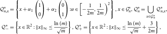 \begin{align*} \mathcal Q^*_{n,x}&=\left \{x+\alpha _1\begin{pmatrix}1\\ 0\end{pmatrix}+\alpha _2\begin{pmatrix}0\\ 1\end{pmatrix}:\alpha \in \left [-\frac {1}{2m},\frac {1}{2m}\right )^2\right \}\textrm {, }x\in \mathcal{G}^*_n\textrm {, } \mathcal Q^*_n=\bigcup _{x\in \mathcal{G}^*_n}\mathcal Q^*_{n,x}\textrm {,}\\ \mathcal Q^*_-&=\left \{x\in \mathbb {R}^2\,:\,\|x\|_\infty \le \frac {\ln (m)}{\sqrt {m}}\right \}\textrm {, } \mathcal Q^*_+=\left \{x\in \mathbb {R}^2\,:\,\|x\|_\infty \le \frac {\ln (m)}{\sqrt {m}}+\frac {3}{2m}\right \}\textrm {, } \end{align*}
and $\mathcal U^*_n\subseteq \mathcal Q^*_-\subseteq \mathcal Q^*_n\subseteq \mathcal Q^*_+\subseteq \mathcal X^*$
for
$\mathcal U^*_n\subseteq \mathcal Q^*_-\subseteq \mathcal Q^*_n\subseteq \mathcal Q^*_+\subseteq \mathcal X^*$
for $n\in \mathcal N$
sufficiently large. Further, with Lemma 5.6 and the definition of
$n\in \mathcal N$
sufficiently large. Further, with Lemma 5.6 and the definition of $\gamma ^{(2)}_d$
we now have
$\gamma ^{(2)}_d$
we now have
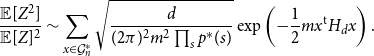 \begin{align*} \frac {\mathbb {E}[Z^2]}{\mathbb {E}[Z]^2}\sim \sum _{x\in \mathcal{G}^*_n}\sqrt {\frac {d}{(2\pi )^2m^2\prod _sp^*(s)}}\exp \left ({-}\frac {1}{2}mx^{\mathrm {t}}H_dx\right ). \end{align*}
Finally, we need to adjust the scaling to turn the sum on the right-hand side into a Riemann sum. For this purpose let $\sigma \,:\,\mathbb {R}^2\rightarrow \mathbb {R}^2$
,
$\sigma \,:\,\mathbb {R}^2\rightarrow \mathbb {R}^2$
, $x\mapsto \sqrt {m}x$
, further
$x\mapsto \sqrt {m}x$
, further $\mathcal{G}^{\prime}_n=\sigma (\mathcal{G}^*_n)$
,
$\mathcal{G}^{\prime}_n=\sigma (\mathcal{G}^*_n)$
, $\mathcal Q^{\prime}_{n,x}=\sigma (\mathcal Q^*_{n,\sigma ^{-1}(x)})$
for
$\mathcal Q^{\prime}_{n,x}=\sigma (\mathcal Q^*_{n,\sigma ^{-1}(x)})$
for $x\in \mathcal{G}^{\prime}_n$
,
$x\in \mathcal{G}^{\prime}_n$
, $\mathcal Q^{\prime}_n=\sigma (\mathcal Q^*_n)$
,
$\mathcal Q^{\prime}_n=\sigma (\mathcal Q^*_n)$
, $\mathcal Q^{\prime}_-=\sigma (\mathcal Q^*_-)$
and
$\mathcal Q^{\prime}_-=\sigma (\mathcal Q^*_-)$
and $\mathcal Q^{\prime}_+=\sigma (\mathcal Q^*_+)$
. This directly gives
$\mathcal Q^{\prime}_+=\sigma (\mathcal Q^*_+)$
. This directly gives
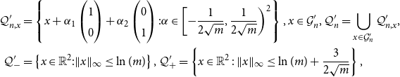 \begin{align*} \mathcal Q^{\prime}_{n,x}&=\left \{x+\alpha _1\begin{pmatrix}1\\ 0\end{pmatrix}+\alpha _2\begin{pmatrix}0\\ 1\end{pmatrix}:\alpha \in \left [-\frac {1}{2\sqrt {m}},\frac {1}{2\sqrt {m}}\right )^2\right \}\textrm {, }x\in \mathcal{G}^{\prime}_n\textrm {, } \mathcal Q^{\prime}_n=\bigcup _{x\in \mathcal{G}^{\prime}_n}\mathcal Q^{\prime}_{n,x}\textrm {,}\\ \mathcal Q^{\prime}_-&=\left \{x\in \mathbb {R}^2:\|x\|_\infty \le \ln (m)\right \}\textrm {, } \mathcal Q^{\prime}_+=\left \{x\in \mathbb {R}^2\,:\,\|x\|_\infty \le \ln (m)+\frac {3}{2\sqrt {m}}\right \}\textrm {, } \end{align*}
and $\mathcal Q^{\prime}_-\subseteq \mathcal Q^{\prime}_n\subseteq \mathcal Q^{\prime}_+$
. Using that
$\mathcal Q^{\prime}_-\subseteq \mathcal Q^{\prime}_n\subseteq \mathcal Q^{\prime}_+$
. Using that $mx^{\mathrm {t}}H_dx=\sigma (x)^{\mathrm {t}}H_d\sigma (x)$
for all
$mx^{\mathrm {t}}H_dx=\sigma (x)^{\mathrm {t}}H_d\sigma (x)$
for all $x\in \mathcal{G}^*_n$
and further that the area of
$x\in \mathcal{G}^*_n$
and further that the area of $\mathcal Q^{\prime}_{n,x}$
is
$\mathcal Q^{\prime}_{n,x}$
is $m^{-1}$
for all
$m^{-1}$
for all $x\in \mathcal{G}^{\prime}_n$
we have
$x\in \mathcal{G}^{\prime}_n$
we have
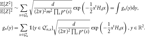 \begin{align*} \frac {\mathbb {E}[Z^2]}{\mathbb {E}[Z]^2}&\sim \sum _{x\in \mathcal{G}^{\prime}_n}\sqrt {\frac {d}{(2\pi )^2m^2\prod _sp^*(s)}}\exp \left ({-}\frac {1}{2}x^{\mathrm {t}}H_dx\right )=\int g_n(y)\mathrm {d}y\textrm {,}\\ g_n(y)&=\sum _{x\in \mathcal{G}^{\prime}_n}\unicode {x1D7D9}\{y\in \mathcal Q^{\prime}_{n,x}\}\sqrt {\frac {d}{(2\pi )^2\prod _sp^*(s)}}\exp \left ({-}\frac {1}{2}x^{\mathrm {t}}H_dx\right )\textrm {, }y\in \mathbb {R}^2\textrm {.} \end{align*}
In order to show that $\int g_n(y)\mathrm {d}y$
converges to
$\int g_n(y)\mathrm {d}y$
converges to $\int g_{\infty }(y)\mathrm {d}y$
we recall from Lemma 5.4 that
$\int g_{\infty }(y)\mathrm {d}y$
we recall from Lemma 5.4 that $H_d$
is positive definite, which ensures that
$H_d$
is positive definite, which ensures that $\int g_{\infty }(y)\mathrm {d}y$
exists and is finite. Now, using Taylor’s theorem with order
$\int g_{\infty }(y)\mathrm {d}y$
exists and is finite. Now, using Taylor’s theorem with order $0$
and the Lagrange form of the first order remainder with the fact that the absolutes of the first derivatives of
$0$
and the Lagrange form of the first order remainder with the fact that the absolutes of the first derivatives of $g_{\infty }$
are bounded from above yields a constant
$g_{\infty }$
are bounded from above yields a constant $c\in \mathbb {R}_{\gt 0}$
such that for all
$c\in \mathbb {R}_{\gt 0}$
such that for all $n\in \mathcal N$
and all
$n\in \mathcal N$
and all $y\in \mathcal Q^{\prime}_n$
, with
$y\in \mathcal Q^{\prime}_n$
, with $x\in \mathcal{G}^{\prime}_n$
such that
$x\in \mathcal{G}^{\prime}_n$
such that $y\in \mathcal Q^{\prime}_{n,x}$
, we have
$y\in \mathcal Q^{\prime}_{n,x}$
, we have
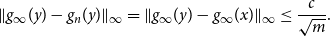 \begin{align*} \|g_{\infty }(y)-g_n(y)\|_{\infty }=\|g_{\infty }(y)-g_{\infty }(x)\|_{\infty }\le \frac {c}{\sqrt {m}}\textrm {.} \end{align*}
This bound directly suggests that
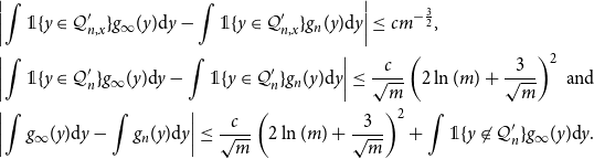 \begin{align*} &\left |\int \unicode {x1D7D9}\{y\in \mathcal Q^{\prime}_{n,x}\}g_{\infty }(y)\mathrm {d}y-\int \unicode {x1D7D9}\{y\in \mathcal Q^{\prime}_{n,x}\}g_{n}(y)\mathrm {d}y\right |\le cm^{-\frac {3}{2}}\textrm {, }\\ &\left |\int \unicode {x1D7D9}\{y\in \mathcal Q^{\prime}_{n}\}g_{\infty }(y)\mathrm {d}y-\int \unicode {x1D7D9}\{y\in \mathcal Q^{\prime}_{n}\}g_{n}(y)\mathrm {d}y\right |\le \frac {c}{\sqrt {m}}\left (2\ln (m)+\frac {3}{\sqrt {m}}\right )^2\textrm { and }\\ &\left |\int g_{\infty }(y)\mathrm {d}y-\int g_{n}(y)\mathrm {d}y\right |\le \frac {c}{\sqrt {m}}\left (2\ln (m)+\frac {3}{\sqrt {m}}\right )^2+\int \unicode {x1D7D9}\{y\not \in \mathcal Q^{\prime}_{n}\}g_{\infty }(y)\mathrm {d}y\textrm {.} \end{align*}
In particular the last bound suggests that $\int g_n(y)\mathrm {d}y\rightarrow \int g_{\infty }(y)\mathrm {d}y$
since the error on the right-hand side tends to zero as
$\int g_n(y)\mathrm {d}y\rightarrow \int g_{\infty }(y)\mathrm {d}y$
since the error on the right-hand side tends to zero as $n$
tends to infinity.
$n$
tends to infinity.
The only remaining part of the proof is to compute $\int g_\infty (x)\mathrm {d}x$
.
$\int g_\infty (x)\mathrm {d}x$
.
Lemma 5.8.
We have $\int g_\infty (x)\mathrm {d}x=\sqrt {\frac {k-1}{k-d}}$
.
$\int g_\infty (x)\mathrm {d}x=\sqrt {\frac {k-1}{k-d}}$
.
Proof. The Gaussian integral gives
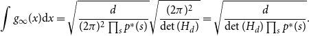 \begin{align*} \int g_\infty (x)\mathrm {d}x =\sqrt {\frac {d}{(2\pi )^2\prod _sp^*(s)}}\sqrt {\frac {(2\pi )^2}{\det (H_d)}} =\sqrt {\frac {d}{\det (H_d)\prod _sp^*(s)}}\textrm {.} \end{align*}
Recall that the Hessian $H_d\in \mathbb {R}^{2\times 2}$
from (6) is a
$H_d\in \mathbb {R}^{2\times 2}$
from (6) is a $2\times 2$
matrix and all entries are given explicitly, so a straightforward calculation asserts that
$2\times 2$
matrix and all entries are given explicitly, so a straightforward calculation asserts that $\det (H_d)=(k-d)d/[(k-1)\prod _sp^*(s)]$
.
$\det (H_d)=(k-d)d/[(k-1)\prod _sp^*(s)]$
.
Finally, combining Lemma 5.7 with Lemma 5.8 completes the proof of Proposition 2.6.
5.6 Proof of Proposition 2.5
This section is dedicated to the identification of the minimizers of $\Delta _d$
. First, we show that the stationary points of
$\Delta _d$
. First, we show that the stationary points of $\Delta _d$
including their characterization are in one to one correspondence with the fixed points of a ratio of belief propagation messages for the constraint satisfaction problem defined in Section 5.1, cf. Lemmas 5.9 to 5.12 below. Considering the ratio turns out to be sufficient and allows to consider a one-dimensional problem. For more background on the correspondence of stationary points of
$\Delta _d$
including their characterization are in one to one correspondence with the fixed points of a ratio of belief propagation messages for the constraint satisfaction problem defined in Section 5.1, cf. Lemmas 5.9 to 5.12 below. Considering the ratio turns out to be sufficient and allows to consider a one-dimensional problem. For more background on the correspondence of stationary points of $\Delta _d$
and fixed points of belief propagation we refer the reader to [Reference Mézard and Montanari31, Reference Yedidia, Freeman and Weiss41].
$\Delta _d$
and fixed points of belief propagation we refer the reader to [Reference Mézard and Montanari31, Reference Yedidia, Freeman and Weiss41].
The major advantage of this equivalent fixed point problem, cf.Equation (9) below, is that the base function $\iota _{\mathrm {BP}}^*$
is a simple rational function and the target function
$\iota _{\mathrm {BP}}^*$
is a simple rational function and the target function $\iota _{\mathrm {BP}}$
is obtained from
$\iota _{\mathrm {BP}}$
is obtained from $\iota _{\mathrm {BP}}^*$
by a single exponentiation. Thus, in the second step we discuss
$\iota _{\mathrm {BP}}^*$
by a single exponentiation. Thus, in the second step we discuss $\iota _{\mathrm {BP}}^*$
and introduce a piecewise linear bound on
$\iota _{\mathrm {BP}}^*$
and introduce a piecewise linear bound on $\iota _{\mathrm {BP}}^*$
on
$\iota _{\mathrm {BP}}^*$
on $[1,k]$
given by
$[1,k]$
given by $g_1^*$
and
$g_1^*$
and $g_k^*$
, cf.Lemma 5.13 below. The piecewise function given by
$g_k^*$
, cf.Lemma 5.13 below. The piecewise function given by $g_1^*$
and
$g_1^*$
and $g_k^*$
on
$g_k^*$
on $[1,k]$
and
$[1,k]$
and $\iota _{\mathrm {BP}}^*$
on
$\iota _{\mathrm {BP}}^*$
on $[k,\infty )$
is increasing and piecewise convex, which allows to establish the unique fixed point of
$[k,\infty )$
is increasing and piecewise convex, which allows to establish the unique fixed point of $\iota _{\mathrm {BP}}$
on
$\iota _{\mathrm {BP}}$
on $(1,\infty )$
(and for reasonable choices of
$(1,\infty )$
(and for reasonable choices of $d$
) in Lemmas 5.16 and 5.17. For symmetry reasons this also completes the discussion for
$d$
) in Lemmas 5.16 and 5.17. For symmetry reasons this also completes the discussion for $k=4$
.
$k=4$
.
In the last step, we establish that $\iota _{\mathrm {BP}}$
has no fixed points on
$\iota _{\mathrm {BP}}$
has no fixed points on $(0,1)$
, for reasonable
$(0,1)$
, for reasonable $d$
and
$d$
and $k\gt 4$
, cf.Lemma 5.19 below. By combining the results we obtain that
$k\gt 4$
, cf.Lemma 5.19 below. By combining the results we obtain that $\iota _{\mathrm {BP}}$
has two fixed points (three for
$\iota _{\mathrm {BP}}$
has two fixed points (three for $k=4$
), one at
$k=4$
), one at $1$
corresponding to the desired interior minimum of
$1$
corresponding to the desired interior minimum of $\Delta _d$
and one in
$\Delta _d$
and one in $[k,\infty )$
corresponding to a saddle point of
$[k,\infty )$
corresponding to a saddle point of $\Delta _d$
(two for
$\Delta _d$
(two for $k=4$
, and for reasonable
$k=4$
, and for reasonable $d$
). This allows to identify the two minimizers of
$d$
). This allows to identify the two minimizers of $\Delta _{d^*}$
(three for
$\Delta _{d^*}$
(three for $k=4$
) and completes the proof.
$k=4$
) and completes the proof.
We begin with characterizing the stationary points of $\Delta _d$
for any
$\Delta _d$
for any $d\in \mathbb {R}_{\gt 0}$
.
$d\in \mathbb {R}_{\gt 0}$
.
In order to pin them down we first determine the stationary points of the restriction of $\Delta _d$
to overlap distributions with the same fixed edge distribution. For this purpose, recall the line
$\Delta _d$
to overlap distributions with the same fixed edge distribution. For this purpose, recall the line $\mathcal W\subseteq \mathcal P(\{0,1\}^2)$
of attainable edge distributions and the lines
$\mathcal W\subseteq \mathcal P(\{0,1\}^2)$
of attainable edge distributions and the lines $\mathcal P_q=\iota (\mathcal X_q)=\{p\in \mathcal P(\{0,1,2\})\,:\,p_{\mathrm {e}}=q\}$
of overlap distributions with fixed edge distribution
$\mathcal P_q=\iota (\mathcal X_q)=\{p\in \mathcal P(\{0,1,2\})\,:\,p_{\mathrm {e}}=q\}$
of overlap distributions with fixed edge distribution $q\in \mathcal W$
from Lemma 5.2. Further, let
$q\in \mathcal W$
from Lemma 5.2. Further, let $\Delta _{d,q}\,:\,\mathcal P_q\rightarrow \mathbb {R}$
denote the restriction of
$\Delta _{d,q}\,:\,\mathcal P_q\rightarrow \mathbb {R}$
denote the restriction of $\Delta _d$
to
$\Delta _d$
to $\mathcal P_q$
. For
$\mathcal P_q$
. For $x\in \mathbb {R}_{\gt 0}$
let
$x\in \mathbb {R}_{\gt 0}$
let $p_x\in \mathcal P(\{0,1,2\})$
be given by
$p_x\in \mathcal P(\{0,1,2\})$
be given by $p_x(s)=p^*(s)x^s/\sum _sp^*(s)x^s$
,
$p_x(s)=p^*(s)x^s/\sum _sp^*(s)x^s$
, $s\in \{0,1,2\}$
, further let
$s\in \{0,1,2\}$
, further let $p_{0}=p^{(0)}$
,
$p_{0}=p^{(0)}$
, $p_{\infty }=p^{(2)}$
, and
$p_{\infty }=p^{(2)}$
, and $\mathcal P_{\min }=\{p_x\,:\,x\in [0,\infty ]\}$
. Finally, let
$\mathcal P_{\min }=\{p_x\,:\,x\in [0,\infty ]\}$
. Finally, let $\iota _{\mathrm {rp}}\,:\,[0,\infty ]\rightarrow \mathcal P_{\min }$
,
$\iota _{\mathrm {rp}}\,:\,[0,\infty ]\rightarrow \mathcal P_{\min }$
, $x\mapsto p_x$
, denote the induced map and
$x\mapsto p_x$
, denote the induced map and $\iota _{\mathrm {pe}}\,:\,\mathcal P_{\min }\rightarrow \mathcal W$
,
$\iota _{\mathrm {pe}}\,:\,\mathcal P_{\min }\rightarrow \mathcal W$
, $p\mapsto p_{\mathrm {e}}$
, the corresponding edge distributions.
$p\mapsto p_{\mathrm {e}}$
, the corresponding edge distributions.
Lemma 5.9.
For all $q\in \mathcal W\setminus \{p^{(0)}_{\mathrm {e}},p^{(2)}_{\mathrm {e}}\}$
the map
$q\in \mathcal W\setminus \{p^{(0)}_{\mathrm {e}},p^{(2)}_{\mathrm {e}}\}$
the map $\Delta _{d,q}$
has a unique stationary point
$\Delta _{d,q}$
has a unique stationary point $p_q\in \mathcal P_q$
that is a global minimum. The unique global minimizer of
$p_q\in \mathcal P_q$
that is a global minimum. The unique global minimizer of $\Delta _{d,p^{(s)}_{\mathrm {e}}}$
is
$\Delta _{d,p^{(s)}_{\mathrm {e}}}$
is $p_{p^{(s)}_{\mathrm {e}}}=p^{(s)}$
for
$p_{p^{(s)}_{\mathrm {e}}}=p^{(s)}$
for $s\in \{0,2\}$
. Further, we have
$s\in \{0,2\}$
. Further, we have $\mathcal P_{\min }=\{p_q:q\in \mathcal W\}$
and the maps
$\mathcal P_{\min }=\{p_q:q\in \mathcal W\}$
and the maps $\iota _{\mathrm {rp}}$
,
$\iota _{\mathrm {rp}}$
, $\iota _{\mathrm {pe}}$
are bijections.
$\iota _{\mathrm {pe}}$
are bijections.
Proof. Recall from Lemma 5.2 that $\mathcal P_q$
is one-dimensional for
$\mathcal P_q$
is one-dimensional for $q\in \mathcal W\setminus \{p^{(0)}_{\mathrm {e}},p^{(2)}_{\mathrm {e}}\}$
. Further, the map
$q\in \mathcal W\setminus \{p^{(0)}_{\mathrm {e}},p^{(2)}_{\mathrm {e}}\}$
. Further, the map $\Delta _{d,q}$
is strictly convex since the KL divergence
$\Delta _{d,q}$
is strictly convex since the KL divergence $D_{\textrm {KL}}(p\parallel p^*)$
(respectively
$D_{\textrm {KL}}(p\parallel p^*)$
(respectively $x\ln (x)$
) is and further
$x\ln (x)$
) is and further $D_{\textrm {KL}}(p_{\mathrm {e}}\parallel p^*_{\mathrm {e}})=D_{\textrm {KL}} (q\parallel p^*_{\mathrm {e}})$
is constant. Now, fix an interior point
$D_{\textrm {KL}}(p_{\mathrm {e}}\parallel p^*_{\mathrm {e}})=D_{\textrm {KL}} (q\parallel p^*_{\mathrm {e}})$
is constant. Now, fix an interior point $p_\circ \in \mathcal P_q$
and let a boundary point
$p_\circ \in \mathcal P_q$
and let a boundary point $p_{\mathrm {b}}\in \mathcal P_q$
be given. Then
$p_{\mathrm {b}}\in \mathcal P_q$
be given. Then $p_{\mathrm {b}}$
is not fully supported since it is on the boundary of
$p_{\mathrm {b}}$
is not fully supported since it is on the boundary of $\mathcal P(\{0,1,2\}$
and hence the derivative of
$\mathcal P(\{0,1,2\}$
and hence the derivative of $D_{\textrm {KL}}(\alpha p_{\circ }+(1-\alpha )p_{\mathrm {b}}\parallel p^*)$
tends to
$D_{\textrm {KL}}(\alpha p_{\circ }+(1-\alpha )p_{\mathrm {b}}\parallel p^*)$
tends to $-\infty$
as
$-\infty$
as $\alpha$
tends to
$\alpha$
tends to $0$
, which shows that
$0$
, which shows that $\Delta _{d,q}$
is not minimized on the boundary. Hence, we know that there exists exactly one stationary point
$\Delta _{d,q}$
is not minimized on the boundary. Hence, we know that there exists exactly one stationary point $p_q\in \mathcal P_q$
and that
$p_q\in \mathcal P_q$
and that $\Delta _{d,q}(p)$
is minimal iff
$\Delta _{d,q}(p)$
is minimal iff $p=p_q$
. As discussed in Lemma 5.2 we have
$p=p_q$
. As discussed in Lemma 5.2 we have $\mathcal P_q=\{p^{(s)}\}$
for
$\mathcal P_q=\{p^{(s)}\}$
for $q=p^{(s)}_{\mathrm {e}}$
and
$q=p^{(s)}_{\mathrm {e}}$
and $s\in \{0,2\}$
, so
$s\in \{0,2\}$
, so $p_q=p^{(s)}$
is obviously the unique global minimizer of
$p_q=p^{(s)}$
is obviously the unique global minimizer of $\Delta _{d,q}$
in this case and further
$\Delta _{d,q}$
in this case and further $\Delta _{d,q}$
has no stationary points (since
$\Delta _{d,q}$
has no stationary points (since $\mathcal P_q$
has empty interior). This shows that the map
$\mathcal P_q$
has empty interior). This shows that the map $q\mapsto p_q$
for
$q\mapsto p_q$
for $q\in \mathcal W$
is a bijection.
$q\in \mathcal W$
is a bijection.
Further, for $q$
in the interior of
$q$
in the interior of $\mathcal W$
the stationary point
$\mathcal W$
the stationary point $p_q$
is fully supported and the unique root of the first derivative of
$p_q$
is fully supported and the unique root of the first derivative of $\Delta _{d,q}$
in the direction
$\Delta _{d,q}$
in the direction $b_2$
from (4), i.e.
$b_2$
from (4), i.e.
 \begin{align*} \ln \left (\frac {p_q(0)}{p^*(0)}\right )+\ln \left (\frac {p_q(2)}{p^*(2)}\right )=2\ln \left (\frac {p_q(1)}{p^*(1)}\right )\textrm { or equivalently } \frac {p_q(2)/p^*(2)}{p_q(1)/p^*(1)}=\frac {p_q(1)/p^*(1)}{p_q(0)/p^*(0)}\textrm {.} \end{align*}
Let $\mathcal P^{\prime}_{\min }$
denote the set of all fully supported
$\mathcal P^{\prime}_{\min }$
denote the set of all fully supported $p\in \mathcal P(\{0,1,2\})$
satisfying
$p\in \mathcal P(\{0,1,2\})$
satisfying $\frac {p(2)/p^*(2)}{p(1)/p^*(1)}=\frac {p(1)/p^*(1)}{p(0)/p^*(0)}$
, i.e. our set of candidates for stationary points. Now, for
$\frac {p(2)/p^*(2)}{p(1)/p^*(1)}=\frac {p(1)/p^*(1)}{p(0)/p^*(0)}$
, i.e. our set of candidates for stationary points. Now, for $p\in \mathcal P^{\prime}_{\min }$
let
$p\in \mathcal P^{\prime}_{\min }$
let $q=p_{\mathrm {e}}$
, then we obviously have
$q=p_{\mathrm {e}}$
, then we obviously have $p\in \mathcal P_q$
and
$p\in \mathcal P_q$
and $p$
is a root of the first derivative of
$p$
is a root of the first derivative of $\Delta _{d,q}$
in the direction
$\Delta _{d,q}$
in the direction $b_2$
, so
$b_2$
, so $p$
is the unique root and
$p$
is the unique root and $p=p_q$
. Hence, the map
$p=p_q$
. Hence, the map $\iota _{\mathrm {pe}}^{\prime}\,:\,\mathcal P^{\prime}_{\min }\rightarrow \mathcal W$
,
$\iota _{\mathrm {pe}}^{\prime}\,:\,\mathcal P^{\prime}_{\min }\rightarrow \mathcal W$
, $p\mapsto p_{\mathrm {e}}$
, is a bijection (up to the corners of
$p\mapsto p_{\mathrm {e}}$
, is a bijection (up to the corners of $\mathcal W$
) with inverse
$\mathcal W$
) with inverse $q\mapsto p_q$
. Now, let
$q\mapsto p_q$
. Now, let $\iota _{\mathrm {pr}}:\mathcal P^{\prime}_{\min }\rightarrow \mathbb {R}_{\gt 0}$
,
$\iota _{\mathrm {pr}}:\mathcal P^{\prime}_{\min }\rightarrow \mathbb {R}_{\gt 0}$
, $p\mapsto x_p$
, with
$p\mapsto x_p$
, with $x_p=\frac {p(1)p^*(0)}{p^*(1)p(0)}$
. Notice that
$x_p=\frac {p(1)p^*(0)}{p^*(1)p(0)}$
. Notice that $\iota _{\mathrm {pr}}$
is surjective since for any
$\iota _{\mathrm {pr}}$
is surjective since for any $x\in \mathbb {R}_{\gt 0}$
we have
$x\in \mathbb {R}_{\gt 0}$
we have
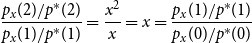 \begin{align*} \frac {p_x(2)/p^*(2)}{p_x(1)/p^*(1)}=\frac {x^2}{x}=x=\frac {p_x(1)/p^*(1)}{p_x(0)/p^*(0)} \end{align*}
and hence $p_x\in \mathcal P^{\prime}_{\min }$
. To show that
$p_x\in \mathcal P^{\prime}_{\min }$
. To show that $\iota _{\mathrm {pr}}$
is injective let
$\iota _{\mathrm {pr}}$
is injective let $p\in \mathcal P^{\prime}_{\min }$
and
$p\in \mathcal P^{\prime}_{\min }$
and $x=x_p$
. Using the definition of
$x=x_p$
. Using the definition of $x_p$
and the defining property of
$x_p$
and the defining property of $\mathcal P^{\prime}_{\min }$
we get
$\mathcal P^{\prime}_{\min }$
we get
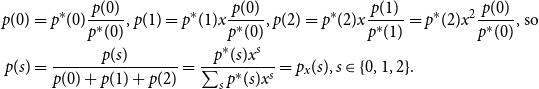 \begin{align*} p(0)&=p^*(0)\frac {p(0)}{p^*(0)}\textrm {, } p(1)=p^*(1)x\frac {p(0)}{p^*(0)}\textrm {, } p(2)=p^*(2)x\frac {p(1)}{p^*(1)}=p^*(2)x^2\frac {p(0)}{p^*(0)}\textrm {, so}\\ p(s)&=\frac {p(s)}{p(0)+p(1)+p(2)}=\frac {p^*(s)x^s}{\sum _sp^*(s)x^s}=p_x(s)\textrm {, }s\in \{0,1,2\}\textrm {.} \end{align*}
This shows that $\mathcal P_{\min }=\mathcal P^{\prime}_{\min }\cup \{p_0,p_\infty \}$
, that
$\mathcal P_{\min }=\mathcal P^{\prime}_{\min }\cup \{p_0,p_\infty \}$
, that $\iota _{\mathrm {rp}}$
is a bijection with inverse
$\iota _{\mathrm {rp}}$
is a bijection with inverse $\iota _{\mathrm {pr}}$
(canonically extended to the endpoints), and finally that
$\iota _{\mathrm {pr}}$
(canonically extended to the endpoints), and finally that $\iota _{\mathrm {pe}}=\iota ^{\prime}_{\mathrm {pe}}$
is a bijection as well.
$\iota _{\mathrm {pe}}=\iota ^{\prime}_{\mathrm {pe}}$
is a bijection as well.
Lemma 5.9 has a few immediate consequences. For one, the only minimizers of $\Delta _d$
in the direction
$\Delta _d$
in the direction $b_2$
, from (4), on the boundary are
$b_2$
, from (4), on the boundary are $p^{(0)}$
and
$p^{(0)}$
and $p^{(2)}$
, while all other boundary points are maximizers in the direction
$p^{(2)}$
, while all other boundary points are maximizers in the direction $b_2$
, hence if
$b_2$
, hence if $p$
is a global minimizer of
$p$
is a global minimizer of $\Delta _d$
on the boundary, we have
$\Delta _d$
on the boundary, we have $p\in \{p^{(0)},p^{(2)}\}$
. Further, all stationary points of
$p\in \{p^{(0)},p^{(2)}\}$
. Further, all stationary points of $\Delta _d$
are either local minima or saddle points. Finally, we have
$\Delta _d$
are either local minima or saddle points. Finally, we have $p\in \mathcal P_{\min }$
for any stationary point
$p\in \mathcal P_{\min }$
for any stationary point $p\in \mathcal P(\{0,1,2\})$
of
$p\in \mathcal P(\{0,1,2\})$
of $\Delta _d$
since then also the derivative in the direction of
$\Delta _d$
since then also the derivative in the direction of $b_2$
vanishes.
$b_2$
vanishes.
For the upcoming characterization of the stationary points of $\Delta _d$
let
$\Delta _d$
let
 \begin{align*} \iota _{\mathrm {rr}}\,:\,\mathbb {R}_{\gt 0}\rightarrow \mathbb {R}_{\gt 0},\quad \iota _{\mathrm {rr}}(x)=\iota ^*_{\mathrm {rr}}(x)^{\frac {d-1}{d}}\textrm {, } \iota ^*_{\mathrm {rr}}(x)=\frac {p_{x,\mathrm {e}}(1,1)p_{x,\mathrm {e}}(0,0)}{p_{x,\mathrm {e}}(1,0)p_{x,\mathrm {e}}(0,1)} \textrm {.} \end{align*}
Notice that $\iota _{\mathrm {rr}}(x)\in \mathbb {R}_{\gt 0}$
for
$\iota _{\mathrm {rr}}(x)\in \mathbb {R}_{\gt 0}$
for $x\in \mathbb {R}_{\gt 0}$
since then
$x\in \mathbb {R}_{\gt 0}$
since then $p_x$
is fully supported and hence
$p_x$
is fully supported and hence $p_{x,\mathrm {e}}$
is fully supported by Lemma 5.2. Finally, let
$p_{x,\mathrm {e}}$
is fully supported by Lemma 5.2. Finally, let $\mathcal X_{\mathrm {st}}=\{x\in \mathbb {R}_{\gt 0}\,:\,\iota _{\mathrm {rr}}(x)=x\}$
denote the fixed points of
$\mathcal X_{\mathrm {st}}=\{x\in \mathbb {R}_{\gt 0}\,:\,\iota _{\mathrm {rr}}(x)=x\}$
denote the fixed points of $\iota _{\mathrm {rr}}$
and
$\iota _{\mathrm {rr}}$
and $\mathcal P_{\mathrm {st}}=\{p_x\,:\,x\in \mathcal X_{\mathrm {st}}\}$
the corresponding distributions. Notice that
$\mathcal P_{\mathrm {st}}=\{p_x\,:\,x\in \mathcal X_{\mathrm {st}}\}$
the corresponding distributions. Notice that $p_x=p^*$
for
$p_x=p^*$
for $x=1$
and further
$x=1$
and further $\iota _{\mathrm {rr}}^*(1)=1$
, i.e.
$\iota _{\mathrm {rr}}^*(1)=1$
, i.e. $\iota _{\mathrm {rr}}(1)=1$
for all
$\iota _{\mathrm {rr}}(1)=1$
for all $d\in \mathbb {R}_{\gt 0}$
, hence
$d\in \mathbb {R}_{\gt 0}$
, hence $1\in \mathcal X_{\mathrm {st}}$
and
$1\in \mathcal X_{\mathrm {st}}$
and $p^*\in \mathcal P_{\mathrm {st}}$
for all
$p^*\in \mathcal P_{\mathrm {st}}$
for all $d\in \mathbb {R}_{\gt 0}$
.
$d\in \mathbb {R}_{\gt 0}$
.
Lemma 5.10.
The stationary points of $\Delta _d$
are given by
$\Delta _d$
are given by $\mathcal P_{\mathrm {st}}$
.
$\mathcal P_{\mathrm {st}}$
.
Proof. Using Lemma 5.9, a fully supported distribution $p\in \mathcal P(\{0,1,2\})$
is a stationary point of
$p\in \mathcal P(\{0,1,2\})$
is a stationary point of $\Delta _d$
iff there exists
$\Delta _d$
iff there exists $x\in \mathbb {R}_{\gt 0}$
such that
$x\in \mathbb {R}_{\gt 0}$
such that $p=p_x$
and the derivative of
$p=p_x$
and the derivative of $\Delta _d$
at
$\Delta _d$
at $p_x$
in the direction
$p_x$
in the direction $b_1$
vanishes, i.e.
$b_1$
vanishes, i.e. $p_x$
is a solution of
$p_x$
is a solution of
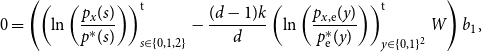 \begin{align*} 0=\left (\left (\ln \left (\frac {p_x(s)}{p^*(s)}\right )\right )_{s\in \{0,1,2\}}^{\mathrm {t}}-\frac {(d-1)k}{d}\left (\ln \left (\frac {p_{x,\mathrm {e}}(y)}{p^*_{\mathrm {e}}(y)}\right )\right )_{y\in \{0,1\}^2}^{\mathrm {t}}W\right )b_1\textrm {,} \end{align*}
where we used the chain rule for multivariate calculus, that $W$
is column stochastic and that
$W$
is column stochastic and that $b_1\in 1_{\{0,1,2\}}^{\perp }$
. Recall from Section 5.3, e.g. from the proof of Lemma 5.1, that
$b_1\in 1_{\{0,1,2\}}^{\perp }$
. Recall from Section 5.3, e.g. from the proof of Lemma 5.1, that $Wb_1=\frac {d}{k}w$
, hence computing the dot product with
$Wb_1=\frac {d}{k}w$
, hence computing the dot product with $b_1$
gives
$b_1$
gives
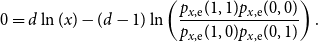 \begin{align*} 0=d\ln (x)-(d-1)\ln \left (\frac {p_{x,\mathrm {e}}(1,1)p_{x,\mathrm {e}}(0,0)}{p_{x,\mathrm {e}}(1,0)p_{x,\mathrm {e}}(0,1)}\right )\textrm {.} \end{align*}
Obviously, equality holds if and only if $x\in \mathcal X_{\mathrm {st}}$
, hence
$x\in \mathcal X_{\mathrm {st}}$
, hence $p$
is a stationary point of
$p$
is a stationary point of $\Delta _d$
iff
$\Delta _d$
iff $p\in \mathcal P_{\mathrm {st}}$
.
$p\in \mathcal P_{\mathrm {st}}$
.
Lemma 5.10 does not only allow to translate the stationary points of $\Delta _d$
into fixed points of
$\Delta _d$
into fixed points of $\iota _{\mathrm {rr}}$
, it also allows to translate the types as follows.
$\iota _{\mathrm {rr}}$
, it also allows to translate the types as follows.
Lemma 5.11.
Fix $x\in \mathbb {R}_{\gt 0}$
. Then we have
$x\in \mathbb {R}_{\gt 0}$
. Then we have $\iota _{\mathrm {rr}}(x)\lt x$
iff
$\iota _{\mathrm {rr}}(x)\lt x$
iff $(\Delta _d\circ \iota _{\mathrm {rp}})^{\prime}(x)\gt 0$
,
$(\Delta _d\circ \iota _{\mathrm {rp}})^{\prime}(x)\gt 0$
, $\iota _{\mathrm {rr}}(x)\gt x$
iff
$\iota _{\mathrm {rr}}(x)\gt x$
iff $(\Delta _d\circ \iota _{\mathrm {rp}})^{\prime}(x)\lt 0$
, and
$(\Delta _d\circ \iota _{\mathrm {rp}})^{\prime}(x)\lt 0$
, and $\iota _{\mathrm {rr}}(x)=x$
iff
$\iota _{\mathrm {rr}}(x)=x$
iff $(\Delta _d\circ \iota _{\mathrm {rp}})^{\prime}(x)=0$
.
$(\Delta _d\circ \iota _{\mathrm {rp}})^{\prime}(x)=0$
.
Proof. Fix $x\in \mathbb {R}_{\gt 0}$
. The proof of Lemma 5.10 directly suggests that the first derivative of
$x\in \mathbb {R}_{\gt 0}$
. The proof of Lemma 5.10 directly suggests that the first derivative of $\Delta _d$
at
$\Delta _d$
at $p_x$
in the direction
$p_x$
in the direction $b_1$
is strictly positive iff
$b_1$
is strictly positive iff
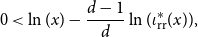 \begin{align*} 0\lt \ln (x)-\frac {d-1}{d}\ln (\iota ^*_{\mathrm {rr}}(x))\textrm {,} \end{align*}
which holds iff $\iota _{\mathrm {rr}}(x)\lt x$
. We’re left to establish that the direction of
$\iota _{\mathrm {rr}}(x)\lt x$
. We’re left to establish that the direction of $\iota _{\mathrm {rp}}$
is consistent with
$\iota _{\mathrm {rp}}$
is consistent with $b_1$
. Intuitively, using Lemma 5.2 and Lemma 5.9 we can argue that
$b_1$
. Intuitively, using Lemma 5.2 and Lemma 5.9 we can argue that $x\mapsto p_{x,\mathrm {e}}(1,1)$
is a bijection and hence either increasing or decreasing. Taking the limits
$x\mapsto p_{x,\mathrm {e}}(1,1)$
is a bijection and hence either increasing or decreasing. Taking the limits $x\rightarrow 0$
and
$x\rightarrow 0$
and $x\rightarrow \infty$
suggests that it is increasing, hence with
$x\rightarrow \infty$
suggests that it is increasing, hence with $c\in \mathbb {R}^2$
given by
$c\in \mathbb {R}^2$
given by $\iota ^{\prime}_{\mathrm {rp}}(x)=(b_1,b_2)c$
, we know that
$\iota ^{\prime}_{\mathrm {rp}}(x)=(b_1,b_2)c$
, we know that $c_1\ge 0$
.
$c_1\ge 0$
.
Formally, we quantify the direction of $\iota _{\mathrm {rp}}$
. For this purpose we compute the derivative of
$\iota _{\mathrm {rp}}$
. For this purpose we compute the derivative of $\iota _{\mathrm {rp}}$
at
$\iota _{\mathrm {rp}}$
at $x\in \mathbb {R}_{\gt 0}$
, given by
$x\in \mathbb {R}_{\gt 0}$
, given by
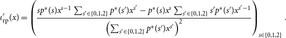 \begin{align*} \iota ^{\prime}_{\mathrm {rp}}(x)=\left (\frac {sp^*(s)x^{s-1}\sum _{s^{\prime}\in \{0,1,2\}}p^*(s^{\prime})x^{s^{\prime}}-p^*(s)x^{s}\sum _{s^{\prime}\in \{0,1,2\}}s^{\prime}p^*(s^{\prime})x^{s^{\prime}-1}}{\left (\sum _{s^{\prime}\in \{0,1,2\}}p^*(s^{\prime})x^{s^{\prime}}\right )^2}\right )_{s\in \{0,1,2\}}\textrm {.} \end{align*}
Notice that $v=\iota ^{\prime}_{\mathrm {rp}}(x)\in 1_{\{0,1,2\}}^{\perp }$
, since
$v=\iota ^{\prime}_{\mathrm {rp}}(x)\in 1_{\{0,1,2\}}^{\perp }$
, since $\iota _{\mathrm {rp}}(\mathbb {R}_{\gt 0})\subseteq \mathcal P(\{0,1,2\})$
or by computing
$\iota _{\mathrm {rp}}(\mathbb {R}_{\gt 0})\subseteq \mathcal P(\{0,1,2\})$
or by computing $\sum _sv_s=0$
directly. Now, let
$\sum _sv_s=0$
directly. Now, let $c\in \mathbb {R}^2$
be given by
$c\in \mathbb {R}^2$
be given by $v=(b_1,b_2)c$
. This directly gives
$v=(b_1,b_2)c$
. This directly gives $c_2=v_2$
and hence
$c_2=v_2$
and hence $c_1=d^{-1}(v_1+2v_2)=d^{-1}\sum _ssv_s$
. Now, notice that
$c_1=d^{-1}(v_1+2v_2)=d^{-1}\sum _ssv_s$
. Now, notice that
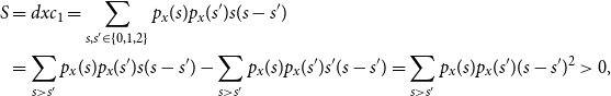 \begin{align*} S&=dxc_1 =\sum _{s,s^{\prime}\in \{0,1,2\}}p_x(s)p_x(s^{\prime})s(s-s^{\prime})\\ &=\sum _{s\gt s^{\prime}}p_x(s)p_x(s^{\prime})s(s-s^{\prime})-\sum _{s\gt s^{\prime}}p_x(s)p_x(s^{\prime})s^{\prime}(s-s^{\prime}) =\sum _{s\gt s^{\prime}}p_x(s)p_x(s^{\prime})(s-s^{\prime})^2\gt 0\textrm {,} \end{align*}
which directly gives $c_1=\frac {S}{dx}\in \mathbb {R}_{\gt 0}$
. Now, with
$c_1=\frac {S}{dx}\in \mathbb {R}_{\gt 0}$
. Now, with $\nabla =\left (\frac {\partial \Delta _d}{\partial p(s)}(p_x)\right )_{s\in \{0,1,2\}}\in \mathbb {R}^{\{0,1,2\}}$
denoting the partial derivatives of
$\nabla =\left (\frac {\partial \Delta _d}{\partial p(s)}(p_x)\right )_{s\in \{0,1,2\}}\in \mathbb {R}^{\{0,1,2\}}$
denoting the partial derivatives of $\Delta _d$
at
$\Delta _d$
at $p_x$
and using the chain rule we have
$p_x$
and using the chain rule we have
 \begin{align*} (\Delta _d\circ \iota _{\mathrm {rp}})^{\prime}(x) &=\nabla ^{\mathrm {t}}\iota ^{\prime}_{\mathrm {rp}}(x) =c_1\nabla ^{\mathrm {t}}b_1 +c_2\nabla ^{\mathrm {t}}b_2 =c_1\nabla ^{\mathrm {t}}b_1\textrm {,} \end{align*}
since the derivative $\nabla ^{\mathrm {t}}b_2$
of
$\nabla ^{\mathrm {t}}b_2$
of $\Delta _d$
at
$\Delta _d$
at $p_x$
in the direction
$p_x$
in the direction $b_2$
is zero, hence we have
$b_2$
is zero, hence we have $(\Delta _d\circ \iota _{\mathrm {rp}})^{\prime}(x)\gt 0$
iff the derivative
$(\Delta _d\circ \iota _{\mathrm {rp}})^{\prime}(x)\gt 0$
iff the derivative $\nabla ^{\mathrm {t}}b_1$
of
$\nabla ^{\mathrm {t}}b_1$
of $\Delta _d$
at
$\Delta _d$
at $p_x$
in the direction
$p_x$
in the direction $b_1$
is strictly positive, which is the case iff
$b_1$
is strictly positive, which is the case iff $\iota _{\mathrm {rr}}(x)\lt x$
.
$\iota _{\mathrm {rr}}(x)\lt x$
.
Lemma 5.11 with Lemma 5.10 shows that control over $\iota _{\mathrm {rr}}$
gives complete control over the location and characterization of the stationary points of
$\iota _{\mathrm {rr}}$
gives complete control over the location and characterization of the stationary points of $\Delta _d$
. However, instead of solving the fixed point equation given by
$\Delta _d$
. However, instead of solving the fixed point equation given by $\iota _{\mathrm {rr}}$
directly, we use a slight modification inspired by the belief propagation algorithm applied to the constraint satisfaction discussed in Section 5.1 and initialized with uniform messages.
$\iota _{\mathrm {rr}}$
directly, we use a slight modification inspired by the belief propagation algorithm applied to the constraint satisfaction discussed in Section 5.1 and initialized with uniform messages.
For this purpose let $N\in \mathbb {Z}_{\ge 0}$
, further
$N\in \mathbb {Z}_{\ge 0}$
, further $N_1$
,
$N_1$
, $N_2\in [N]_0$
and the hypergeometric distribution
$N_2\in [N]_0$
and the hypergeometric distribution $p_{N,N_1,N_2}\in \mathcal P(\mathbb {Z})$
be given by
$p_{N,N_1,N_2}\in \mathcal P(\mathbb {Z})$
be given by
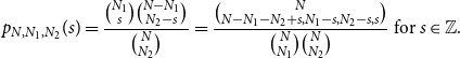 \begin{align*} p_{N,N_1,N_2}(s)=\frac {\binom {N_1}{s}\binom {N-N_1}{N_2-s}}{\binom {N}{N_2}}=\frac {\binom {N}{N-N_1-N_2+s,N_1-s,N_2-s,s}}{\binom {N}{N_1}\binom {N}{N_2}}\textrm { for }s\in \mathbb {Z}\textrm {.} \end{align*}
The latter form directly shows that $p_{N,N_1,N_2}=p_{N,N_2,N_1}$
. Now, for
$p_{N,N_1,N_2}=p_{N,N_2,N_1}$
. Now, for $y\in \{0,1\}^2$
let
$y\in \{0,1\}^2$
let $p^*_y\in \mathcal P(\{0,1,2\})$
be given by
$p^*_y\in \mathcal P(\{0,1,2\})$
be given by $p^*_{(1,1)}(s)=p_{k-1,1,1}(s-1)$
,
$p^*_{(1,1)}(s)=p_{k-1,1,1}(s-1)$
, $p^*_{(1,0)}(s)=p_{k-1,1,2}(s)$
,
$p^*_{(1,0)}(s)=p_{k-1,1,2}(s)$
, $p^*_{(0,1)}(s)=p_{k-1,2,1}(s)$
,
$p^*_{(0,1)}(s)=p_{k-1,2,1}(s)$
, $p^*_{(0,0)}(s)=p_{k-1,2,2}(s)$
for
$p^*_{(0,0)}(s)=p_{k-1,2,2}(s)$
for $s\in \{0,1,2\}$
. On the other hand, for
$s\in \{0,1,2\}$
. On the other hand, for $y\in \{0,1\}^2$
let
$y\in \{0,1\}^2$
let $p^{\prime}_y\in \mathcal P(\{0,1,2\})$
be given by
$p^{\prime}_y\in \mathcal P(\{0,1,2\})$
be given by $p^{\prime}_{(1,1)}(s)=p_{k-1,1,1}(s)$
for
$p^{\prime}_{(1,1)}(s)=p_{k-1,1,1}(s)$
for $s\in \{0,1,2\}$
and further
$s\in \{0,1,2\}$
and further $p^{\prime}_y=p^*_y$
for
$p^{\prime}_y=p^*_y$
for $y\in \{0,1\}^2\setminus \{(1,1)\}$
. Finally, for a distribution
$y\in \{0,1\}^2\setminus \{(1,1)\}$
. Finally, for a distribution $p\in \mathcal P(\{0,1,2\})$
let
$p\in \mathcal P(\{0,1,2\})$
let $f_p\,:\,\mathbb {R}_{\ge 0}\rightarrow \mathbb {R}_{\ge 0}$
,
$f_p\,:\,\mathbb {R}_{\ge 0}\rightarrow \mathbb {R}_{\ge 0}$
, $x\mapsto \sum _{s\in \{0,1,2\}}p(s)x^s$
, be its probability generating function, and further
$x\mapsto \sum _{s\in \{0,1,2\}}p(s)x^s$
, be its probability generating function, and further $\iota _{\mathrm {BP}}\,:\,\mathbb {R}_{\gt 0}\rightarrow \mathbb {R}_{\gt 0}$
given by
$\iota _{\mathrm {BP}}\,:\,\mathbb {R}_{\gt 0}\rightarrow \mathbb {R}_{\gt 0}$
given by
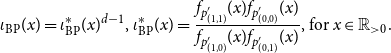 \begin{align} \iota _{\mathrm {BP}}(x)=\iota ^*_{\mathrm {BP}}(x)^{d-1}\textrm {, } \iota ^*_{\mathrm {BP}}(x)=\frac {f_{p^{\prime}_{(1,1)}}(x)f_{p^{\prime}_{(0,0)}}(x)}{f_{p^{\prime}_{(1,0)}}(x)f_{p^{\prime}_{(0,1)}}(x)}\textrm {, for }x\in \mathbb {R}_{\gt 0}\textrm {.} \end{align}
Lemma 5.12.
Fix $x\in \mathbb {R}_{\gt 0}$
. Then we have
$x\in \mathbb {R}_{\gt 0}$
. Then we have $\iota _{\mathrm {rr}}(x)\lt x$
iff
$\iota _{\mathrm {rr}}(x)\lt x$
iff $\iota _{\mathrm {BP}}(x)\lt x$
,
$\iota _{\mathrm {BP}}(x)\lt x$
, $\iota _{\mathrm {rr}}(x)\gt x$
iff
$\iota _{\mathrm {rr}}(x)\gt x$
iff $\iota _{\mathrm {BP}}(x)\gt x$
, and
$\iota _{\mathrm {BP}}(x)\gt x$
, and $\iota _{\mathrm {rr}}(x)=x$
iff
$\iota _{\mathrm {rr}}(x)=x$
iff $\iota _{\mathrm {BP}}(x)=x$
.
$\iota _{\mathrm {BP}}(x)=x$
.
Proof. First, notice that the normalization constant of $p_x$
cancels out in
$p_x$
cancels out in $\iota ^*_{\mathrm {rr}}$
, as does the normalization constant
$\iota ^*_{\mathrm {rr}}$
, as does the normalization constant $\binom {k}{2}^2$
of
$\binom {k}{2}^2$
of $p^*$
. Further, with
$p^*$
. Further, with $v=(k-4+s,2-s,2-s,s)^{\mathrm {t}}\in \mathbb {R}^{\{0,1\}^2}$
we have
$v=(k-4+s,2-s,2-s,s)^{\mathrm {t}}\in \mathbb {R}^{\{0,1\}^2}$
we have $W_{y,s}\binom {k}{v}=\frac {v_y}{k}\binom {k}{v}=\binom {k-1}{v-(\delta _{y,z})_z}$
for
$W_{y,s}\binom {k}{v}=\frac {v_y}{k}\binom {k}{v}=\binom {k-1}{v-(\delta _{y,z})_z}$
for $y\in \{0,1\}^2$
,
$y\in \{0,1\}^2$
, $s\in \{0,1,2\}$
, and thereby
$s\in \{0,1,2\}$
, and thereby
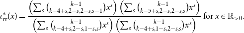 \begin{align*} \iota ^*_{\mathrm {rr}}(x)=\frac {\left (\sum _s\binom {k-1}{k-4+s,2-s,2-s,s-1}x^s\right )\left (\sum _s\binom {k-1}{k-5+s,2-s,2-s,s}x^s\right )}{\left (\sum _s\binom {k-1}{k-4+s,2-s,1-s,s}x^s\right )\left (\sum _s\binom {k-1}{k-4+s,1-s,2-s,s}x^s\right )} \textrm { for }x\in \mathbb {R}_{\gt 0}. \end{align*}
Now, since the normalization constants cancel out in total, this directly gives
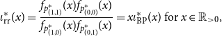 \begin{align*} \iota ^*_{\mathrm {rr}}(x)=\frac {f_{p^*_{(1,1)}}(x)f_{p^*_{(0,0)}}(x)}{f_{p^*_{(1,0)}}(x)f_{p^*_{(0,1)}}(x)} =x\iota ^*_{\mathrm {BP}}(x) \textrm { for }x\in \mathbb {R}_{\gt 0}\textrm {,} \end{align*}
using that $p^*_{(1,1)}(s)=p^{\prime}_{(1,1)}(s-1)$
for
$p^*_{(1,1)}(s)=p^{\prime}_{(1,1)}(s-1)$
for $s\in \{0,1,2\}$
, hence
$s\in \{0,1,2\}$
, hence $f_{p^*_{(1,1)}}(x)=xf_{p^{\prime}_{(1,1)}}(x)$
, and
$f_{p^*_{(1,1)}}(x)=xf_{p^{\prime}_{(1,1)}}(x)$
, and $p^*_y(s)=p^{\prime}_y(s)$
for
$p^*_y(s)=p^{\prime}_y(s)$
for $y\neq (1,1)$
. Now, we have
$y\neq (1,1)$
. Now, we have $x=\iota _{\mathrm {rr}}(x)$
iff
$x=\iota _{\mathrm {rr}}(x)$
iff $x=x^{\frac {d-1}{d}}\iota _{\mathrm {BP}}(x)^{\frac {1}{d}}$
, which holds iff
$x=x^{\frac {d-1}{d}}\iota _{\mathrm {BP}}(x)^{\frac {1}{d}}$
, which holds iff $x^{\frac {1}{d}}=\iota _{\mathrm {BP}}(x)^{\frac {1}{d}}$
, which then again is equivalent to
$x^{\frac {1}{d}}=\iota _{\mathrm {BP}}(x)^{\frac {1}{d}}$
, which then again is equivalent to $x=\iota _{\mathrm {BP}}(x)$
. Equivalence of the inequalities follows analogously.
$x=\iota _{\mathrm {BP}}(x)$
. Equivalence of the inequalities follows analogously.
The following part is dedicated to the identification of the fixed points of $\iota _{\mathrm {BP}}$
. We start with a discussion of
$\iota _{\mathrm {BP}}$
. We start with a discussion of $\iota ^*_{\mathrm {BP}}$
. For this purpose let
$\iota ^*_{\mathrm {BP}}$
. For this purpose let $g^*_1$
,
$g^*_1$
, $g^*_k\,:\,\mathbb {R}_{\ge 1}\rightarrow \mathbb {R}_{\ge 1}$
be given by
$g^*_k\,:\,\mathbb {R}_{\ge 1}\rightarrow \mathbb {R}_{\ge 1}$
be given by
 \begin{align*} g^*_1(x)=\frac {1}{k-1}(x-1)+1\textrm { and } g^*_k(x)=\frac {13k-12}{27(k-1)(k-2)}(x-k)+\frac {2(7k-12)}{9(k-2)}\textrm {, }x\in \mathbb {R}_{\ge 1}\textrm {.} \end{align*}
Lemma 5.13.
For any $k\in \mathbb {Z}_{\ge 4}$
we have
$k\in \mathbb {Z}_{\ge 4}$
we have
 \begin{align*} \lim _{x\rightarrow 0}\iota ^*_{\mathrm {BP}}(x)=\frac {k-4}{k-3}\textrm {, } \quad \iota ^*_{\mathrm {BP}}(1)=1=g^*_1(1)\quad \textrm {and} \quad \iota ^*_{\mathrm {BP}}(k)=g^*_k(k)\textrm {.} \end{align*}
For the first derivative we have
 \begin{align*} {\iota ^*}^{\prime}_{\mathrm {BP}}(1)={g^*}^{\prime}_1(1)\textrm {, } \quad {\iota ^*}^{\prime}_{\mathrm {BP}}(k)={g^*}^{\prime}_k(k)\quad \textrm {and} \quad \lim _{x\rightarrow \infty }{\iota ^*}^{\prime}_{\mathrm {BP}}(x)=\frac {1}{2(k-2)}\textrm {.} \end{align*}
Moreover, for the second derivative we have
 \begin{align*} {\iota ^*}^{\prime\prime}_{\mathrm {BP}}(x)\lt 0\textrm { for }x\in (0,k)\textrm {, } \quad {\iota ^*}^{\prime\prime}_{\mathrm {BP}}(k)=0\textrm {,} \quad {\iota ^*}^{\prime\prime}_{\mathrm {BP}}(x)\gt 0\textrm { for }x\in \mathbb {R}_{\gt k}\textrm {.} \end{align*}
For $k=4$
and
$k=4$
and $x\in \mathbb {R}_{\gt 0}$
we have
$x\in \mathbb {R}_{\gt 0}$
we have $\iota ^*_{\mathrm {BP}}(x^{-1})=\left (\iota ^*_{\mathrm {BP}}(x)\right )^{-1}$
.
$\iota ^*_{\mathrm {BP}}(x^{-1})=\left (\iota ^*_{\mathrm {BP}}(x)\right )^{-1}$
.
Proof. Using $f_p(1)=1$
for the moment generating function of any finitely supported law
$f_p(1)=1$
for the moment generating function of any finitely supported law $p$
, we have
$p$
, we have $\iota ^*_{\mathrm {BP}}(1)=1$
. Further, using that the first moment of a hypergeometric distribution
$\iota ^*_{\mathrm {BP}}(1)=1$
. Further, using that the first moment of a hypergeometric distribution $p_{N,N_1,N_2}$
is
$p_{N,N_1,N_2}$
is $\frac {N_1N_2}{N}$
and that
$\frac {N_1N_2}{N}$
and that $f^{\prime}_p(1)$
is the first moment of
$f^{\prime}_p(1)$
is the first moment of $p$
, we have
$p$
, we have ${\iota ^*}^{\prime}_{\mathrm {BP}}(1)=\frac {1}{k-1}+\frac {4}{k-1}-2\cdot \frac {2}{k-1}=\frac {1}{k-1}$
. The symmetry of
${\iota ^*}^{\prime}_{\mathrm {BP}}(1)=\frac {1}{k-1}+\frac {4}{k-1}-2\cdot \frac {2}{k-1}=\frac {1}{k-1}$
. The symmetry of $\iota ^*_{\mathrm {BP}}$
for the special case
$\iota ^*_{\mathrm {BP}}$
for the special case $k=4$
can be seen as follows. First, recall that
$k=4$
can be seen as follows. First, recall that $p_{N,N_1,N_2}(s)=p_{N,N-N_1,N_2}(N_2-s)$
for any hypergeometric distribution
$p_{N,N_1,N_2}(s)=p_{N,N-N_1,N_2}(N_2-s)$
for any hypergeometric distribution $p_{N,N_1,N_2}$
. For
$p_{N,N_1,N_2}$
. For $s\in \{0,1,2\}$
this gives
$s\in \{0,1,2\}$
this gives
 \begin{align*} p^{\prime}_{(0,0)}(s)&=p_{3,2,2}(s)=p_{3,1,2}(2-s)=p^{\prime}_{(1,0)}(2-s)\\ &=p^{\prime}_{(0,1)}(2-s)=p_{3,2,1}(2-s)=p_{3,1,1}(s-1)=p^{\prime}_{(1,1)}(s-1)\textrm {.} \end{align*}
These relations can be directly translated to the moment generating functions, i.e.
 \begin{align*} f_{p^{\prime}_{(0,0)}}(x)&=x^2f_{p^{\prime}_{(1,0)}}(x^{-1})=x^2f_{p^{\prime}_{(0,1)}}(x^{-1})=xf_{p^{\prime}_{(1,1)}}(x) \end{align*}
for $x\in \mathbb {R}_{\gt 0}$
. Using these transformations we have
$x\in \mathbb {R}_{\gt 0}$
. Using these transformations we have
 \begin{align*} \iota ^*_{\mathrm {BP}}(x^{-1}) =\frac {f_{p^{\prime}_{(1,1)}}(x^{-1})f_{p^{\prime}_{(0,0)}}(x^{-1})}{f_{p^{\prime}_{(1,0)}}(x^{-1})f_{p^{\prime}_{(0,1)}}(x^{-1})} =\frac {x^{-1}f_{p^{\prime}_{(1,0)}}(x)x^{-2}f_{p^{\prime}_{(0,1)}}(x)}{x^{-1}f_{p^{\prime}_{(1,1)}}(x)x^{-2}f_{p^{\prime}_{(0,0)}}(x)} =\left (\iota ^*_{\mathrm {BP}}(x)\right )^{-1}\textrm {.} \end{align*}
For $k\in \mathbb {Z}_{\ge 4}$
and
$k\in \mathbb {Z}_{\ge 4}$
and $x\in \mathbb {R}_{\gt 0}$
direct computation gives
$x\in \mathbb {R}_{\gt 0}$
direct computation gives
 \begin{align*} \iota ^*_{\mathrm {BP}}(x)&=\frac {1}{2(k-2)}x+\frac {2k-5}{2(k-2)}+\frac {(k-1)(k-3)(x-1)}{2(k-2)(2x+k-3)^2}\textrm {,}\\ {\iota ^*}^{\prime}_{\mathrm {BP}}(x)&=\frac {1}{2(k-2)}+\frac {(k-1)(k-3)({-}2x+k+1)}{2(k-2)(2x+k-3)^3}\textrm {,}\\ {\iota ^*}^{\prime\prime}_{\mathrm {BP}}(x)&=\frac {4(k-1)(k-3)(x-k)}{(k-2)(2x+k-3)^4}\textrm {.} \end{align*}
The remaining assertions follow immediately or with routine computations.
Lemma 5.13 has the following immediate consequences.
Corollary 5.14.
For any $d\in (0,2]$
we have
$d\in (0,2]$
we have $\iota ^*_{\mathrm {BP}}\in (x,1)$
for
$\iota ^*_{\mathrm {BP}}\in (x,1)$
for $x\in (0,1)$
and
$x\in (0,1)$
and $\iota ^*_{\mathrm {BP}}(x)\in (1,x)$
for
$\iota ^*_{\mathrm {BP}}(x)\in (1,x)$
for $x\in \mathbb {R}_{\gt 1}$
. In particular,
$x\in \mathbb {R}_{\gt 1}$
. In particular, $p^*$
is the unique minimizer of
$p^*$
is the unique minimizer of $\Delta _d$
.
$\Delta _d$
.
Proof. Using Lemma 5.13 we notice that ${\iota ^*}^{\prime}_{\mathrm {BP}}(x)\in [{\iota ^*}^{\prime}_{\mathrm {BP}}(k),\frac {1}{k-1}]\subset (0,1)$
for
${\iota ^*}^{\prime}_{\mathrm {BP}}(x)\in [{\iota ^*}^{\prime}_{\mathrm {BP}}(k),\frac {1}{k-1}]\subset (0,1)$
for $x\in \mathbb {R}_{\ge 1}$
and
$x\in \mathbb {R}_{\ge 1}$
and $\iota ^*_{\mathrm {BP}}(x)=x$
for
$\iota ^*_{\mathrm {BP}}(x)=x$
for $x=1$
, hence we have
$x=1$
, hence we have $\iota ^*_{\mathrm {BP}}(x)\in (1,x)$
for
$\iota ^*_{\mathrm {BP}}(x)\in (1,x)$
for $x\in \mathbb {R}_{\gt 1}$
. For
$x\in \mathbb {R}_{\gt 1}$
. For $k=4$
this gives
$k=4$
this gives $\iota ^*_{\mathrm {BP}}(x)\in (x,1)$
using the symmetry result. For
$\iota ^*_{\mathrm {BP}}(x)\in (x,1)$
using the symmetry result. For $k\in \mathbb {Z}_{\gt 4}$
we have
$k\in \mathbb {Z}_{\gt 4}$
we have $\lim _{x\rightarrow 0}\iota ^*_{\mathrm {BP}}(x)\gt 0$
, which gives
$\lim _{x\rightarrow 0}\iota ^*_{\mathrm {BP}}(x)\gt 0$
, which gives $x^*=\inf \{x\in \mathbb {R}_{\gt 0}:\iota ^*_{\mathrm {BP}}(x)\le x\}\in (0,1]$
using
$x^*=\inf \{x\in \mathbb {R}_{\gt 0}:\iota ^*_{\mathrm {BP}}(x)\le x\}\in (0,1]$
using $\iota ^*_{\mathrm {BP}}(1)=1$
. Assume that
$\iota ^*_{\mathrm {BP}}(1)=1$
. Assume that $x^*\lt 1$
, then using the continuity of
$x^*\lt 1$
, then using the continuity of $x-\iota ^*_{\mathrm {BP}}(x)$
we directly get
$x-\iota ^*_{\mathrm {BP}}(x)$
we directly get $\iota ^*_{\mathrm {BP}}(x^*)=x^*$
, and further
$\iota ^*_{\mathrm {BP}}(x^*)=x^*$
, and further ${\iota ^*}^{\prime}_{\mathrm {BP}}(x^*)\le 1$
since
${\iota ^*}^{\prime}_{\mathrm {BP}}(x^*)\le 1$
since $\iota ^*_{\mathrm {BP}}(x)\gt x$
for
$\iota ^*_{\mathrm {BP}}(x)\gt x$
for $x\in (0,x^*)$
. But then, since
$x\in (0,x^*)$
. But then, since ${\iota ^*}^{\prime\prime}_{\mathrm {BP}}(x)\lt 0$
for
${\iota ^*}^{\prime\prime}_{\mathrm {BP}}(x)\lt 0$
for $x\in (0,k)$
, this implies that
$x\in (0,k)$
, this implies that ${\iota ^*}^{\prime}_{\mathrm {BP}}(x)\lt 1$
for
${\iota ^*}^{\prime}_{\mathrm {BP}}(x)\lt 1$
for $x\in (x^*,1]$
which yields that
$x\in (x^*,1]$
which yields that ${\iota ^*}_{\mathrm {BP}}(1)\lt 1$
and hence a contradiction. This shows that
${\iota ^*}_{\mathrm {BP}}(1)\lt 1$
and hence a contradiction. This shows that $\iota ^*_{\mathrm {BP}}(x)\in (x,1)$
for
$\iota ^*_{\mathrm {BP}}(x)\in (x,1)$
for $x\in (0,1)$
. Now, for any
$x\in (0,1)$
. Now, for any $d\in (0,2]$
we have
$d\in (0,2]$
we have $\iota _{\mathrm {BP}}(x)\ge \iota ^*_{\mathrm {BP}}(x)\in (x,1)$
for
$\iota _{\mathrm {BP}}(x)\ge \iota ^*_{\mathrm {BP}}(x)\in (x,1)$
for $x\in (0,1)$
and
$x\in (0,1)$
and $\iota _{\mathrm {BP}}(x)\le \iota ^*_{\mathrm {BP}}(x)\in (1,x)$
for
$\iota _{\mathrm {BP}}(x)\le \iota ^*_{\mathrm {BP}}(x)\in (1,x)$
for $x\in \mathbb {R}_{\gt 1}$
. Hence, using Lemma 5.11 and Lemma 5.12 we immediately get that
$x\in \mathbb {R}_{\gt 1}$
. Hence, using Lemma 5.11 and Lemma 5.12 we immediately get that $p^*=p_1$
is the unique minimizer of
$p^*=p_1$
is the unique minimizer of $\Delta _d$
.
$\Delta _d$
.
Corollary 5.14 covers the case of simple graphs that was discussed in [Reference Robalewska37]. On the other hand, Corollary 5.14 suggests that Proposition 2.5 can only hold if $d^*\gt 2$
.
$d^*\gt 2$
.
Corollary 5.15.
For all $k\in \mathbb {Z}_{\ge 4}$
we have
$k\in \mathbb {Z}_{\ge 4}$
we have $d^*\in \mathbb {R}_{\gt 2}$
.
$d^*\in \mathbb {R}_{\gt 2}$
.
Proof. For $d\in \mathbb {R}_{\gt 0}$
let
$d\in \mathbb {R}_{\gt 0}$
let $f(d)=(\Delta _d\circ \iota _{\mathrm {rp}})(\infty )$
and notice that
$f(d)=(\Delta _d\circ \iota _{\mathrm {rp}})(\infty )$
and notice that $f(d)=\frac {k}{d}\phi _1$
. Corollary 5.14 shows that
$f(d)=\frac {k}{d}\phi _1$
. Corollary 5.14 shows that $f(d)\gt 0$
for all
$f(d)\gt 0$
for all $d\in (0,2]$
. On the other hand, as derived in Section 4 we know that
$d\in (0,2]$
. On the other hand, as derived in Section 4 we know that $d^*$
is the unique root of
$d^*$
is the unique root of $f$
, which shows that
$f$
, which shows that $d^*\gt 2$
.
$d^*\gt 2$
.
Based on Corollary 5.14 we can restrict to $d\in \mathbb {R}_{\gt 2}$
, while Corollary 5.15 motivates the discussion of this interval. Further, the restriction
$d\in \mathbb {R}_{\gt 2}$
, while Corollary 5.15 motivates the discussion of this interval. Further, the restriction $d\in \mathbb {R}_{\gt 2}$
ensures that
$d\in \mathbb {R}_{\gt 2}$
ensures that $x^{d-1}$
is increasing and convex on
$x^{d-1}$
is increasing and convex on $\mathbb {R}_{\gt 0}$
. In the following we will consider the intervals
$\mathbb {R}_{\gt 0}$
. In the following we will consider the intervals $\mathbb {R}_{\ge k}$
,
$\mathbb {R}_{\ge k}$
, $[\bar x,k]$
,
$[\bar x,k]$
, $[1,\bar x]$
and
$[1,\bar x]$
and $(0,1]$
independently, where
$(0,1]$
independently, where $\bar x=\frac {1}{7}(k+6)\in (1,k)$
is the intersection of
$\bar x=\frac {1}{7}(k+6)\in (1,k)$
is the intersection of $g_1$
and
$g_1$
and $g_k$
with
$g_k$
with $g_1(\bar x)=g_k(\bar x)=\frac {8}{7}$
.
$g_1(\bar x)=g_k(\bar x)=\frac {8}{7}$
.
Lemma 5.16.
For $d\in (2,d_k)$
, with
$d\in (2,d_k)$
, with $d_k=\frac {\ln (k)}{\ln (\iota ^*_{\mathrm {BP}}(k))}+1$
, there exists
$d_k=\frac {\ln (k)}{\ln (\iota ^*_{\mathrm {BP}}(k))}+1$
, there exists $x_{\max }\in \mathbb {R}_{\gt k}$
such that
$x_{\max }\in \mathbb {R}_{\gt k}$
such that $\iota _{\mathrm {BP}}(x)\lt x$
for
$\iota _{\mathrm {BP}}(x)\lt x$
for $x\in [k,x_{\max })$
,
$x\in [k,x_{\max })$
, $\iota _{\mathrm {BP}}(x_{\max })=x_{\max }$
and
$\iota _{\mathrm {BP}}(x_{\max })=x_{\max }$
and $\iota _{\mathrm {BP}}(x)\gt x$
for
$\iota _{\mathrm {BP}}(x)\gt x$
for $x\in \mathbb {R}_{\gt x_{\max }}$
.
$x\in \mathbb {R}_{\gt x_{\max }}$
.
Proof. Let $f(d)=\left (\iota _{\mathrm {BP}}^*(k)\right )^{d-1}$
for
$f(d)=\left (\iota _{\mathrm {BP}}^*(k)\right )^{d-1}$
for $d\in \mathbb {R}_{\ge 2}$
, i.e.
$d\in \mathbb {R}_{\ge 2}$
, i.e. $f(d)=\iota _{\mathrm {BP}}(k)$
is the value of
$f(d)=\iota _{\mathrm {BP}}(k)$
is the value of $\iota _{\mathrm {BP}}$
at
$\iota _{\mathrm {BP}}$
at $k$
under a variation of
$k$
under a variation of $d$
. We know from Lemma 5.13 that
$d$
. We know from Lemma 5.13 that $\iota _{\mathrm {BP}}^*(k)\in \mathbb {R}_{\gt 1}$
, hence
$\iota _{\mathrm {BP}}^*(k)\in \mathbb {R}_{\gt 1}$
, hence $f(d)$
is strictly increasing, and further direct computation gives
$f(d)$
is strictly increasing, and further direct computation gives $f(d_k)=k$
, so we have
$f(d_k)=k$
, so we have $\iota _{\mathrm {BP}}(k)\lt k$
for any
$\iota _{\mathrm {BP}}(k)\lt k$
for any $d\in (2,d_k)$
. Now, since
$d\in (2,d_k)$
. Now, since $\iota ^*_{\mathrm {BP}}$
is strictly increasing and convex on
$\iota ^*_{\mathrm {BP}}$
is strictly increasing and convex on $\mathbb {R}_{\gt k}$
by Lemma 5.13 and further the function
$\mathbb {R}_{\gt k}$
by Lemma 5.13 and further the function $x^{d-1}$
is increasing and convex for
$x^{d-1}$
is increasing and convex for $d\in (2,d_k)$
, we know that
$d\in (2,d_k)$
, we know that $\iota _{\mathrm {BP}}$
is convex and increasing on
$\iota _{\mathrm {BP}}$
is convex and increasing on $\mathbb {R}_{\gt k}$
, or formally
$\mathbb {R}_{\gt k}$
, or formally
 \begin{align*} \iota ^{\prime}_{\mathrm {BP}}(x)&=(d-1)\iota ^{*}_{\mathrm {BP}}(x)^{d-2}{\iota ^*}^{\prime}_{\mathrm {BP}}(x)=(d-1)\iota _{\mathrm {BP}}(x)\frac {{\iota ^*}^{\prime}_{\mathrm {BP}}(x)}{\iota ^*_{\mathrm {BP}}(x)}\gt 0\textrm {, }\\ \iota ^{\prime\prime}_{\mathrm {BP}}(x)&=(d-1)\iota _{\mathrm {BP}}(x)\left [(d-2)\left (\frac {{\iota ^*}^{\prime}_{\mathrm {BP}}(x)}{\iota ^*_{\mathrm {BP}}(x)}\right )^2+\frac {{\iota ^*}^{\prime\prime}_{\mathrm {BP}}(x)}{\iota ^*_{\mathrm {BP}}(x)}\right ]\gt 0\textrm {.} \end{align*}
Using Lemma 5.13 and for $x\rightarrow \infty$
we have
$x\rightarrow \infty$
we have $\iota ^{*}_{\mathrm {BP}}(x)\rightarrow \infty$
since
$\iota ^{*}_{\mathrm {BP}}(x)\rightarrow \infty$
since ${\iota ^*}^{\prime}_{\mathrm {BP}}(x)\rightarrow \frac {1}{2(k-2)}$
and hence
${\iota ^*}^{\prime}_{\mathrm {BP}}(x)\rightarrow \frac {1}{2(k-2)}$
and hence $\iota ^{\prime}_{\mathrm {BP}}(x)\rightarrow \infty$
by the above, i.e.
$\iota ^{\prime}_{\mathrm {BP}}(x)\rightarrow \infty$
by the above, i.e. $\iota _{\mathrm {BP}}(x)-x\rightarrow \infty$
, which suggests the existence of
$\iota _{\mathrm {BP}}(x)-x\rightarrow \infty$
, which suggests the existence of $x_{\max }\in \mathbb {R}_{\gt k}$
with
$x_{\max }\in \mathbb {R}_{\gt k}$
with $\iota _{\mathrm {BP}}(x_{\max })=x_{\max }$
since
$\iota _{\mathrm {BP}}(x_{\max })=x_{\max }$
since $\iota _{\mathrm {BP}}(k)\lt k$
. Now, let
$\iota _{\mathrm {BP}}(k)\lt k$
. Now, let $x_+=\inf \{x\in \mathbb {R}_{\ge k}:\iota _{\mathrm {BP}}(x)\ge x\}$
, then we have
$x_+=\inf \{x\in \mathbb {R}_{\ge k}:\iota _{\mathrm {BP}}(x)\ge x\}$
, then we have $x_+\in (k,x_{\max }]$
. Since
$x_+\in (k,x_{\max }]$
. Since $\iota _{\mathrm {BP}}(x)\lt x$
for
$\iota _{\mathrm {BP}}(x)\lt x$
for $x\in [k,x_+)$
we need
$x\in [k,x_+)$
we need $\iota ^{\prime}_{\mathrm {BP}}(x_+)\ge 1$
, which gives
$\iota ^{\prime}_{\mathrm {BP}}(x_+)\ge 1$
, which gives $\iota ^{\prime}_{\mathrm {BP}}(x)\gt 1$
for
$\iota ^{\prime}_{\mathrm {BP}}(x)\gt 1$
for $x\gt x_+$
since
$x\gt x_+$
since $\iota ^{\prime\prime}_{\mathrm {BP}}(x)\gt 0$
, hence
$\iota ^{\prime\prime}_{\mathrm {BP}}(x)\gt 0$
, hence $\iota _{\mathrm {BP}}(x)\gt x$
, thereby
$\iota _{\mathrm {BP}}(x)\gt x$
, thereby $x_+=x_{\max }$
, and in summary
$x_+=x_{\max }$
, and in summary $\iota _{\mathrm {BP}}(x)\lt x$
for
$\iota _{\mathrm {BP}}(x)\lt x$
for $x\in [k,x_{\max })$
,
$x\in [k,x_{\max })$
, $\iota _{\mathrm {BP}}(x_{\max })=x_{\max }$
and
$\iota _{\mathrm {BP}}(x_{\max })=x_{\max }$
and $\iota _{\mathrm {BP}}(x)\gt x$
for
$\iota _{\mathrm {BP}}(x)\gt x$
for $x\in \mathbb {R}_{\gt x_{\max }}$
.
$x\in \mathbb {R}_{\gt x_{\max }}$
.
The proof of Lemma 5.16 serves as a blueprint for the next two cases, where we do not consider $\iota _{\mathrm {BP}}$
directly since
$\iota _{\mathrm {BP}}$
directly since ${\iota ^*}^{\prime\prime}_{\mathrm {BP}}(x)\lt 0$
on
${\iota ^*}^{\prime\prime}_{\mathrm {BP}}(x)\lt 0$
on $(1,k)$
, but work with
$(1,k)$
, but work with $g_k(x)=g^*_k(x)^{d-1}$
and
$g_k(x)=g^*_k(x)^{d-1}$
and $g_1(x)=g^*_1(x)^{d-1}$
instead, which are convex, increasing and upper bounds for
$g_1(x)=g^*_1(x)^{d-1}$
instead, which are convex, increasing and upper bounds for $\iota _{\mathrm {BP}}$
on
$\iota _{\mathrm {BP}}$
on $[1,k]$
since
$[1,k]$
since ${\iota ^*}^{\prime\prime}_{\mathrm {BP}}(x)\lt 0$
on
${\iota ^*}^{\prime\prime}_{\mathrm {BP}}(x)\lt 0$
on $(1,k)$
. In the spirit of Lemma 5.16 we continue to consider the maximal domain for
$(1,k)$
. In the spirit of Lemma 5.16 we continue to consider the maximal domain for $d\in \mathbb {R}_{\gt 2}$
. Let
$d\in \mathbb {R}_{\gt 2}$
. Let
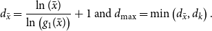 \begin{align*} d_{\bar x}=\frac {\ln (\bar x)}{\ln \left (g_1(\bar x)\right )}+1\textrm { and } d_{\max }=\min \left (d_{\bar x},d_k\right )\textrm {.} \end{align*}
We postpone the proof that $d^*\le d_{\max }$
, instead we focus on the interval
$d^*\le d_{\max }$
, instead we focus on the interval $(1,k)$
.
$(1,k)$
.
Lemma 5.17.
For any $d\in (2,d_{\max })\subseteq (2,k)$
and all
$d\in (2,d_{\max })\subseteq (2,k)$
and all $x\in (1,k]$
we have
$x\in (1,k]$
we have $\iota _{\mathrm {BP}}(x)\lt x$
.
$\iota _{\mathrm {BP}}(x)\lt x$
.
Proof. Fix $d\in (2,d_{\max })$
. Since
$d\in (2,d_{\max })$
. Since ${\iota ^*}^{\prime\prime}_{\mathrm {BP}}(x)\lt 0$
for
${\iota ^*}^{\prime\prime}_{\mathrm {BP}}(x)\lt 0$
for $x\in [1,k)$
, we know that
$x\in [1,k)$
, we know that $\iota ^*_{\mathrm {BP}}(x)\le g^*_k(x)$
for
$\iota ^*_{\mathrm {BP}}(x)\le g^*_k(x)$
for $x\in [\bar x,k]$
and
$x\in [\bar x,k]$
and $\iota ^*_{\mathrm {BP}}(x)\le g^*_1(x)$
for
$\iota ^*_{\mathrm {BP}}(x)\le g^*_1(x)$
for $x\in [1,\bar x]$
, so using that
$x\in [1,\bar x]$
, so using that $x^{d-1}$
is increasing we have that
$x^{d-1}$
is increasing we have that $\iota _{\mathrm {BP}}(x)\le g_k(x)$
for
$\iota _{\mathrm {BP}}(x)\le g_k(x)$
for $x\in [\bar x,k]$
and
$x\in [\bar x,k]$
and $\iota _{\mathrm {BP}}(x)\le g_1(x)$
for
$\iota _{\mathrm {BP}}(x)\le g_1(x)$
for $x\in [1,\bar x]$
. Analogous to Lemma 5.16 we notice that
$x\in [1,\bar x]$
. Analogous to Lemma 5.16 we notice that $g_k(k)=\iota _{\mathrm {BP}}(k)\lt k$
since
$g_k(k)=\iota _{\mathrm {BP}}(k)\lt k$
since $d\lt d_k$
, that
$d\lt d_k$
, that $g_k(\bar x)=g_1(\bar x)\lt \bar x$
since
$g_k(\bar x)=g_1(\bar x)\lt \bar x$
since $d\lt d_{\bar x}$
and that
$d\lt d_{\bar x}$
and that $g_1(1)=1$
. Further, since
$g_1(1)=1$
. Further, since $g^*_1$
,
$g^*_1$
, $g^*_k$
are increasing and convex, using that
$g^*_k$
are increasing and convex, using that $x^{d-1}$
is increasing and convex yields that
$x^{d-1}$
is increasing and convex yields that $g_1$
,
$g_1$
, $g_k$
are increasing and convex. In particular, we can upper bound
$g_k$
are increasing and convex. In particular, we can upper bound $g_k$
with the line
$g_k$
with the line $l_k:[\bar x,k]\rightarrow [g_k(\bar x),g_k(k)]$
connecting
$l_k:[\bar x,k]\rightarrow [g_k(\bar x),g_k(k)]$
connecting $(\bar x,g_k(\bar x))$
and
$(\bar x,g_k(\bar x))$
and $(k,g_k(k))$
, which is entirely and strictly under the diagonal. Analogously, we can upper bound
$(k,g_k(k))$
, which is entirely and strictly under the diagonal. Analogously, we can upper bound $g_1$
with the line
$g_1$
with the line $l_1:[1,\bar x]\rightarrow [1,g_1(\bar x)]$
connecting
$l_1:[1,\bar x]\rightarrow [1,g_1(\bar x)]$
connecting $(1,1)$
and
$(1,1)$
and $(\bar x,g_1(\bar x))$
, which is also entirely and strictly under the diagonal except for
$(\bar x,g_1(\bar x))$
, which is also entirely and strictly under the diagonal except for $(1,1)$
where the two lines intersect. In total,
$(1,1)$
where the two lines intersect. In total, $\iota _{\mathrm {BP}}(x)\le \min (g_1(x),g_k(x))\le \min (l_1(x),l_k(x))\lt x$
for all
$\iota _{\mathrm {BP}}(x)\le \min (g_1(x),g_k(x))\le \min (l_1(x),l_k(x))\lt x$
for all $x\in (1,k]$
. Finally, another implication is that
$x\in (1,k]$
. Finally, another implication is that $\frac {d-1}{k-1}=g^{\prime}_1(1)\le l^{\prime}_1(1)\lt 1$
since
$\frac {d-1}{k-1}=g^{\prime}_1(1)\le l^{\prime}_1(1)\lt 1$
since $l_1$
is below the diagonal, which suggests that
$l_1$
is below the diagonal, which suggests that $d_{\max }\le k$
.
$d_{\max }\le k$
.
Combining Lemma 5.16 and Lemma 5.17 shows for any $d\in (2,d_{\max })$
that
$d\in (2,d_{\max })$
that $\Delta _d\circ \iota _{\mathrm {rp}}$
has exactly one stationary point
$\Delta _d\circ \iota _{\mathrm {rp}}$
has exactly one stationary point $x_{\max }$
on
$x_{\max }$
on $\mathbb {R}_{\gt 1}$
which is the unique maximizer of
$\mathbb {R}_{\gt 1}$
which is the unique maximizer of $\Delta _d\circ \iota _{\mathrm {rp}}$
on this interval. Further, since
$\Delta _d\circ \iota _{\mathrm {rp}}$
on this interval. Further, since $d_{\max }\le k$
and using
$d_{\max }\le k$
and using $\iota ^{\prime}_{\mathrm {BP}}(1)=\frac {d-1}{k-1}$
we also know that
$\iota ^{\prime}_{\mathrm {BP}}(1)=\frac {d-1}{k-1}$
we also know that $x=1$
is an isolated minimizer of
$x=1$
is an isolated minimizer of $\Delta _d\circ \iota _{\mathrm {rp}}$
. Aside, notice that this argumentation can be used to show that
$\Delta _d\circ \iota _{\mathrm {rp}}$
. Aside, notice that this argumentation can be used to show that $H_d$
as defined in Section 5.5 is positive semidefinite for all
$H_d$
as defined in Section 5.5 is positive semidefinite for all $d\lt k$
, hence with the arguments from the proof of Lemma 5.4 we see that
$d\lt k$
, hence with the arguments from the proof of Lemma 5.4 we see that $H_d$
is positive definite for all
$H_d$
is positive definite for all $d\lt k$
and finally with Lemma 5.8 that
$d\lt k$
and finally with Lemma 5.8 that $\eta _{\chi ^2}=\frac {1}{k-1}$
.
$\eta _{\chi ^2}=\frac {1}{k-1}$
.
For the low overlap region $x\in (0,1)$
we need a significantly different approach, since
$x\in (0,1)$
we need a significantly different approach, since $\iota ^*_{\mathrm {BP}}$
is increasing and concave, but
$\iota ^*_{\mathrm {BP}}$
is increasing and concave, but $\iota _{\mathrm {BP}}(x)\lt \iota ^*_{\mathrm {BP}}(x)$
and we need to show that
$\iota _{\mathrm {BP}}(x)\lt \iota ^*_{\mathrm {BP}}(x)$
and we need to show that $\iota _{\mathrm {BP}}(x)\gt x$
. This means that first order approximations as used for
$\iota _{\mathrm {BP}}(x)\gt x$
. This means that first order approximations as used for $(1,k)$
are useless since they are upper bounds to
$(1,k)$
are useless since they are upper bounds to $\iota ^*_{\mathrm {BP}}$
and there are no immediate implications for
$\iota ^*_{\mathrm {BP}}$
and there are no immediate implications for $\iota ^{\prime\prime}_{\mathrm {BP}}$
as was the case for
$\iota ^{\prime\prime}_{\mathrm {BP}}$
as was the case for $\mathbb {R}_{\gt k}$
. However, the symmetric case
$\mathbb {R}_{\gt k}$
. However, the symmetric case $k=4$
can be discussed easily.
$k=4$
can be discussed easily.
Corollary 5.18.
For $k=4$
and
$k=4$
and $d\in (2,d_{\max })$
we have
$d\in (2,d_{\max })$
we have $\iota _{\mathrm {BP}}(x)\lt x$
for
$\iota _{\mathrm {BP}}(x)\lt x$
for $x\in (0,x_{\max }^{-1})$
,
$x\in (0,x_{\max }^{-1})$
, $\iota _{\mathrm {BP}}(x_{\max }^{-1})=x_{\max }^{-1}$
, and
$\iota _{\mathrm {BP}}(x_{\max }^{-1})=x_{\max }^{-1}$
, and $\iota _{\mathrm {BP}}(x)\gt x$
for
$\iota _{\mathrm {BP}}(x)\gt x$
for $x\in (x_{\max }^{-1},1)$
.
$x\in (x_{\max }^{-1},1)$
.
Proof. Combining Lemma 5.17 and Lemma 5.16 we have $\iota _{\mathrm {BP}}(x)\lt x$
for
$\iota _{\mathrm {BP}}(x)\lt x$
for $x\in (1,x_{\max })$
and
$x\in (1,x_{\max })$
and $\iota _{\mathrm {BP}}(x)\gt x$
for
$\iota _{\mathrm {BP}}(x)\gt x$
for $x\in (x_{\max },\infty )$
, hence using the symmetry from Lemma 5.13 directly gives the result.
$x\in (x_{\max },\infty )$
, hence using the symmetry from Lemma 5.13 directly gives the result.
Corollary 5.18 allows to restrict to $k\in \mathbb {Z}_{\gt 4}$
in the remainder. Now, we basically reverse the method used for the interval
$k\in \mathbb {Z}_{\gt 4}$
in the remainder. Now, we basically reverse the method used for the interval $(1,k)$
, i.e. instead of using tangents
$(1,k)$
, i.e. instead of using tangents $g^*_1$
,
$g^*_1$
, $g^*_k$
to
$g^*_k$
to $\iota ^*_{\mathrm {BP}}$
and scaling them with
$\iota ^*_{\mathrm {BP}}$
and scaling them with $(d-1)$
, we scale
$(d-1)$
, we scale $\iota ^*_{\mathrm {BP}}$
such that the diagonal is a tangent, meaning we consider
$\iota ^*_{\mathrm {BP}}$
such that the diagonal is a tangent, meaning we consider $\iota _k=\iota _{\mathrm {BP}}$
for
$\iota _k=\iota _{\mathrm {BP}}$
for $d=k$
since
$d=k$
since $\iota ^{\prime}_{\mathrm {BP}}(1)=\frac {d-1}{k-1}$
, and show that
$\iota ^{\prime}_{\mathrm {BP}}(1)=\frac {d-1}{k-1}$
, and show that $\iota _k$
is sufficiently convex to ensure
$\iota _k$
is sufficiently convex to ensure $\iota _k(x)\gt x$
for
$\iota _k(x)\gt x$
for $x\in (0,1)$
. The next lemma ensures that this approach is applicable for all
$x\in (0,1)$
. The next lemma ensures that this approach is applicable for all $k\ge 5$
.
$k\ge 5$
.
Lemma 5.19.
For any $k\in \mathbb {Z}_{\ge 5}$
,
$k\in \mathbb {Z}_{\ge 5}$
, $d\in (2,k]$
and all
$d\in (2,k]$
and all $x\in (0,1)$
we have
$x\in (0,1)$
we have $\iota _{\mathrm {BP}}(x)\gt x$
.
$\iota _{\mathrm {BP}}(x)\gt x$
.
Proof. Let $k\in \mathbb {Z}_{\ge 5}$
. As derived in the proof of Lemma 5.17 we have
$k\in \mathbb {Z}_{\ge 5}$
. As derived in the proof of Lemma 5.17 we have $\iota _k(1)=1$
and
$\iota _k(1)=1$
and $\iota ^{\prime}_k(1)=1$
, i.e. the diagonal is a tangent to
$\iota ^{\prime}_k(1)=1$
, i.e. the diagonal is a tangent to $\iota _k$
at
$\iota _k$
at $x=1$
. Further, as discussed in the proof of Lemma 5.16,
$x=1$
. Further, as discussed in the proof of Lemma 5.16,
 \begin{align*} \iota ^{\prime\prime}_k(x) &=(k-1)\frac {\iota _k(x)}{\iota ^*_{\mathrm {BP}}(x)^2} \left [(k-2){\iota ^*}^{\prime}_{\mathrm {BP}}(x)^2+\iota ^*_{\mathrm {BP}}(x){\iota ^*}^{\prime\prime}_{\mathrm {BP}}(x)\right ]\textrm { for }x\in (0,1)\textrm {.} \end{align*}
Since the leading factor is clearly strictly positive, we may focus on the term in the square brackets. Further, using that moment generating functions are strictly positive for strictly positive real numbers we can extract the strictly positive denominator of the term and normalize to get
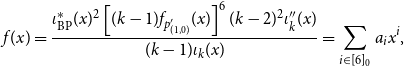 \begin{align*} f(x)&=\frac {\iota ^*_{\mathrm {BP}}(x)^2\left [(k-1)f_{p^{\prime}_{(1,0)}}(x)\right ]^6(k-2)^2\iota ^{\prime\prime}_k(x)}{(k-1)\iota _k(x)}=\sum _{i\in [6]_0}a_ix^i\textrm {,} \end{align*}
where
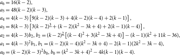 \begin{align*} a_6&=16(k-2)\textrm {,}\\ a_5&=48(k-2)(k-3)\textrm {,}\\ a_4&=4(k-3)\left [9(k-2)(k-3)+4(k-2)(k-4)+2(k-1)\right ]\textrm {,}\\ a_3&=8(k-3)\left [3(k-2)^{\underline {3}}+(k-2)(k^2-3k+4)+2(k-1)(k-4)\right ]\textrm {,}\\ a_2&=4(k-3)b_2\textrm {, } b_2=(k-2)^{\underline {2}}\left [(k-4)^2+3(k^2-3k+4)\right ]-(k-1)(k^2+11k-36)\textrm {,}\\ a_1&=4(k-3)^2b_1\textrm {, }b_1=(k-2)(k-4)(k^2-3k+4)-2(k-1)(2k^2-3k-4)\textrm {,}\\ a_0&=(k-2)(k-3)^2b_0\textrm {, } b_0=(k^2-3k+4)^2-4k(k-1)(k-4)\textrm {.} \end{align*}
We can easily verify that $a_i\gt 0$
for
$a_i\gt 0$
for $3 \le i \le 6$
using that
$3 \le i \le 6$
using that $x^2-3x+4\gt 0$
for all
$x^2-3x+4\gt 0$
for all $x\in \mathbb {R}$
. Viewing the
$x\in \mathbb {R}$
. Viewing the $b_i$
,
$b_i$
, $i\in \{0,1,2\}$
, as polynomials
$i\in \{0,1,2\}$
, as polynomials $b_i(x)$
,
$b_i(x)$
, $x\in \mathbb {R}$
, of degree
$x\in \mathbb {R}$
, of degree $4$
and evaluated at
$4$
and evaluated at $x=k$
, we have
$x=k$
, we have
 \begin{align*} b^{\prime\prime}_2(x)=48x^2-228x+254\textrm {, }b_2(5)=82\textrm {, }b^{\prime}_2(5)=225\textrm {,} \end{align*}
hence $b^{\prime\prime}_2(x)\gt 0$
for
$b^{\prime\prime}_2(x)\gt 0$
for $x\gt x_2$
with
$x\gt x_2$
with $x_2=\frac {19}{8}+\frac {\sqrt {201}}{24}\lt 3$
and by that
$x_2=\frac {19}{8}+\frac {\sqrt {201}}{24}\lt 3$
and by that $b_2(x)\gt 0$
for all
$b_2(x)\gt 0$
for all $x\in \mathbb {R}_{\ge 5}$
, so in particular
$x\in \mathbb {R}_{\ge 5}$
, so in particular $b_2=b_2(k)\gt 0$
since
$b_2=b_2(k)\gt 0$
since $k\in \mathbb {Z}_{\ge 5}$
and thereby
$k\in \mathbb {Z}_{\ge 5}$
and thereby $a_2\gt 0$
. Using the same technique for the degree four polynomials
$a_2\gt 0$
. Using the same technique for the degree four polynomials $b_1(x)$
we obtain that
$b_1(x)$
we obtain that $b^{\prime\prime}_1(x)\gt 0$
for
$b^{\prime\prime}_1(x)\gt 0$
for $x\gt x_1$
with
$x\gt x_1$
with $x_1=\frac {13}{4}+\frac {\sqrt {561}}{12}\lt 6$
,
$x_1=\frac {13}{4}+\frac {\sqrt {561}}{12}\lt 6$
, $b_1(10)=564$
,
$b_1(10)=564$
, $b^{\prime}_1(10)=854$
, and hence that
$b^{\prime}_1(10)=854$
, and hence that $b_1\gt 0$
if
$b_1\gt 0$
if $k\ge 10$
. For
$k\ge 10$
. For $b_0(x)$
we have
$b_0(x)$
we have $b^{\prime\prime}_0(x)\gt 0$
for
$b^{\prime\prime}_0(x)\gt 0$
for $x\gt x_0$
with
$x\gt x_0$
with $x_0=\frac {5}{2}+\frac {\sqrt {3}}{6}\lt 3$
,
$x_0=\frac {5}{2}+\frac {\sqrt {3}}{6}\lt 3$
, $b^{\prime}_0(3)=20$
,
$b^{\prime}_0(3)=20$
, $b_0(3)=40$
, so
$b_0(3)=40$
, so $b_0\gt 0$
for all
$b_0\gt 0$
for all $k\in \mathbb {Z}_{\ge 5}$
.
$k\in \mathbb {Z}_{\ge 5}$
.
Hence, for $k\in \mathbb {Z}_{\ge 10}$
we know that
$k\in \mathbb {Z}_{\ge 10}$
we know that $a_i\gt 0$
for all
$a_i\gt 0$
for all $i\in [6]_0$
, which directly implies that
$i\in [6]_0$
, which directly implies that $f(x)\gt 0$
for all
$f(x)\gt 0$
for all $x\in \mathbb {R}_{\gt 0}$
, so
$x\in \mathbb {R}_{\gt 0}$
, so $\iota ^{\prime\prime}_k(x)\gt 0$
, further
$\iota ^{\prime\prime}_k(x)\gt 0$
, further $\iota ^{\prime}_k(x)\lt 1$
for
$\iota ^{\prime}_k(x)\lt 1$
for $x\in (0,1)$
,
$x\in (0,1)$
, $\iota ^{\prime}_k(x)\gt 1$
for
$\iota ^{\prime}_k(x)\gt 1$
for $x\in \mathbb {R}_{\gt 1}$
and thereby
$x\in \mathbb {R}_{\gt 1}$
and thereby $\iota _k(x)\gt x$
for
$\iota _k(x)\gt x$
for $x\in \mathbb {R}_{\gt 0}\setminus \{1\}$
.
$x\in \mathbb {R}_{\gt 0}\setminus \{1\}$
.
For $5\le k\le 9$
we still have
$5\le k\le 9$
we still have $a_i\gt 0$
for
$a_i\gt 0$
for $i\in [6]_0\setminus \{1\}$
. For
$i\in [6]_0\setminus \{1\}$
. For $6\le k\le 9$
we consider the quadratic function
$6\le k\le 9$
we consider the quadratic function $g_k(x)=\sum _{i\in \{0,1,2\}}a_ix^i$
explicitly, given by
$g_k(x)=\sum _{i\in \{0,1,2\}}a_ix^i$
explicitly, given by
 \begin{align*} g_6(x)=6120x^2-11664x+8784\textrm {, } g_7(x)=24960x^2-25344x+41600\textrm {, }\\ g_8(x)=72560x^2-34400x+156000\textrm {, } g_9(x)=172944x^2-9504x+484848\textrm {.} \end{align*}
It turns out that $g_k(x)\gt 0$
for all
$g_k(x)\gt 0$
for all $x\in \mathbb {R}$
and
$x\in \mathbb {R}$
and $6\le k\le 9$
, which in particular yields
$6\le k\le 9$
, which in particular yields $f(x)\gt 0$
for all
$f(x)\gt 0$
for all $x\in \mathbb {R}_{\gt 0}$
. Using the same argumentation as for
$x\in \mathbb {R}_{\gt 0}$
. Using the same argumentation as for $k\in \mathbb {Z}_{\ge 10}$
shows that
$k\in \mathbb {Z}_{\ge 10}$
shows that $\iota _k(x)\gt x$
for all
$\iota _k(x)\gt x$
for all $x\in \mathbb {R}_{\gt 0}\setminus \{1\}$
and
$x\in \mathbb {R}_{\gt 0}\setminus \{1\}$
and $k\in \mathbb {Z}_{\ge 6}$
.
$k\in \mathbb {Z}_{\ge 6}$
.
As opposed to the previous cases the function $\iota _k$
is not convex for
$\iota _k$
is not convex for $k=5$
, and while this slightly complicates the computation, we will show that this does not affect the overall picture. Now, we consider the complete sixth order polynomial
$k=5$
, and while this slightly complicates the computation, we will show that this does not affect the overall picture. Now, we consider the complete sixth order polynomial
 \begin{align*} f(x)=48x^6 + 288x^5 + 592x^4 + 1088x^3 + 656x^2 - 3296x + 1392\textrm {.} \end{align*}
We notice that $f^{\prime\prime}(x)\gt 0$
for all
$f^{\prime\prime}(x)\gt 0$
for all $x\in \mathbb {R}_{\ge 0}$
since
$x\in \mathbb {R}_{\ge 0}$
since $a_i\gt 0$
for
$a_i\gt 0$
for $i\in [6]\setminus \{1\}$
, hence
$i\in [6]\setminus \{1\}$
, hence $f^{\prime}(x)$
is strictly increasing for
$f^{\prime}(x)$
is strictly increasing for $x\in \mathbb {R}_{\ge 0}$
, which shows the existence of a unique root
$x\in \mathbb {R}_{\ge 0}$
, which shows the existence of a unique root $x_{\min }\in (0,1)$
, using
$x_{\min }\in (0,1)$
, using $f^{\prime}(0)\lt 0$
and
$f^{\prime}(0)\lt 0$
and $f^{\prime}(1)\gt 0$
, i.e.
$f^{\prime}(1)\gt 0$
, i.e. $x_{\min }$
is the unique minimizer of
$x_{\min }$
is the unique minimizer of $f$
on
$f$
on $\mathbb {R}_{\ge 0}$
. Computing
$\mathbb {R}_{\ge 0}$
. Computing $f(x_{1-})\gt 0$
,
$f(x_{1-})\gt 0$
, $f(x_{1+})\lt 0$
and
$f(x_{1+})\lt 0$
and $f(1)\gt 0$
with
$f(1)\gt 0$
with $x_{1-}=0.581$
and
$x_{1-}=0.581$
and $x_{1+}=0.582$
ensures the existence of exactly two roots
$x_{1+}=0.582$
ensures the existence of exactly two roots $x_1\in (x_{1-},x_{1+})$
and
$x_1\in (x_{1-},x_{1+})$
and $x_2\in (x_{1+},1)$
of
$x_2\in (x_{1+},1)$
of $f$
, hence
$f$
, hence $\iota _k$
is convex on
$\iota _k$
is convex on $(0,x_1)$
, concave on
$(0,x_1)$
, concave on $(x_1,x_2)$
and convex on
$(x_1,x_2)$
and convex on $\mathbb {R}_{\gt x_2}$
. Let
$\mathbb {R}_{\gt x_2}$
. Let $g\,:\,\mathbb {R}\rightarrow \mathbb {R}$
,
$g\,:\,\mathbb {R}\rightarrow \mathbb {R}$
, $x\mapsto \iota ^{\prime}_k(x_{1-})(x-x_{1-})+\iota _k(x_{1-})$
denote the tangent of
$x\mapsto \iota ^{\prime}_k(x_{1-})(x-x_{1-})+\iota _k(x_{1-})$
denote the tangent of $\iota _k$
at
$\iota _k$
at $x_{1-}$
. Since we can write both
$x_{1-}$
. Since we can write both $\iota _k$
and
$\iota _k$
and $\iota ^{\prime}_k$
as the ratio of polynomials with integer coefficients, we can compute
$\iota ^{\prime}_k$
as the ratio of polynomials with integer coefficients, we can compute $\iota _k(x_{1-})\in (0.584,0.585)$
,
$\iota _k(x_{1-})\in (0.584,0.585)$
, $\iota ^{\prime}_k(x_{1-})\in (0.99,0.991)$
and
$\iota ^{\prime}_k(x_{1-})\in (0.99,0.991)$
and $g(x_{1+})\in (0.585,0.586)$
exactly. Using the convexity of
$g(x_{1+})\in (0.585,0.586)$
exactly. Using the convexity of $\iota _k$
on
$\iota _k$
on $(0,x_1)$
,
$(0,x_1)$
, $g^{\prime}=\iota ^{\prime}_k(x_{1-})\lt 1$
and
$g^{\prime}=\iota ^{\prime}_k(x_{1-})\lt 1$
and $g(x_{1+})\gt x_{1+}$
immediately gives that
$g(x_{1+})\gt x_{1+}$
immediately gives that $\iota _k(x)\ge g(x)\gt x$
for
$\iota _k(x)\ge g(x)\gt x$
for $x\in (0,x_1]$
. The fact that
$x\in (0,x_1]$
. The fact that $\iota _k(x)\gt x$
for
$\iota _k(x)\gt x$
for $x\in [x_2,1)$
immediately follows from the convexity of
$x\in [x_2,1)$
immediately follows from the convexity of $\iota _k$
on
$\iota _k$
on $(x_2,1)$
and that the diagonal is a tangent to
$(x_2,1)$
and that the diagonal is a tangent to $\iota _k$
at
$\iota _k$
at $x=1$
. But now, since
$x=1$
. But now, since $(x_1,\iota _k(x_1))$
and
$(x_1,\iota _k(x_1))$
and $(x_2,\iota _k(x_2))$
are above the diagonal, so is the line connecting the two, which is a lower bound to
$(x_2,\iota _k(x_2))$
are above the diagonal, so is the line connecting the two, which is a lower bound to $\iota _k$
on
$\iota _k$
on $(x_1,x_2)$
since
$(x_1,x_2)$
since $\iota _k$
is concave on this interval. By that we have finally showed that the overall picture is also the same for
$\iota _k$
is concave on this interval. By that we have finally showed that the overall picture is also the same for $k=5$
, i.e.
$k=5$
, i.e. $\iota _k(x)\gt x$
for
$\iota _k(x)\gt x$
for $x\in \mathbb {R}_{\gt 0}\setminus \{1\}$
.
$x\in \mathbb {R}_{\gt 0}\setminus \{1\}$
.
The fact that $\iota _k(x)\gt x$
, i.e.
$\iota _k(x)\gt x$
, i.e. $\iota _{\mathrm {BP}}(x)\gt x$
with
$\iota _{\mathrm {BP}}(x)\gt x$
with $d=k$
, for
$d=k$
, for $x\in \mathbb {R}_{\gt 0}\setminus \{1\}$
shows that the only stationary point of
$x\in \mathbb {R}_{\gt 0}\setminus \{1\}$
shows that the only stationary point of $\Delta _k$
is a saddle at
$\Delta _k$
is a saddle at $p^*$
(respectively a maximum of
$p^*$
(respectively a maximum of $\Delta _k\circ \iota _{\mathrm {rp}}$
at
$\Delta _k\circ \iota _{\mathrm {rp}}$
at $x=1$
). But more importantly, since
$x=1$
). But more importantly, since $x^{d-1}$
is decreasing in
$x^{d-1}$
is decreasing in $d$
for
$d$
for $x\in (0,1)$
and
$x\in (0,1)$
and $\iota ^*_{\mathrm {BP}}(x)\in (0,1)$
, we have
$\iota ^*_{\mathrm {BP}}(x)\in (0,1)$
, we have $\iota _{\mathrm {BP}}(x)\ge \iota _k(x)\gt x$
for all
$\iota _{\mathrm {BP}}(x)\ge \iota _k(x)\gt x$
for all $d\in (2,k]$
.
$d\in (2,k]$
.
The combination of Lemma 5.16, Lemma 5.17 and Lemma 5.18 shows that for $k=4$
and all
$k=4$
and all $d\in (2,d_{\max })$
there exist exactly three fixed points
$d\in (2,d_{\max })$
there exist exactly three fixed points $x_-\lt x_0\lt x_+$
of
$x_-\lt x_0\lt x_+$
of $\iota _{\mathrm {BP}}$
, with
$\iota _{\mathrm {BP}}$
, with $x_0=1$
,
$x_0=1$
, $x_+\in (k,\infty )$
and
$x_+\in (k,\infty )$
and $x_-=x_+^{-1}$
, hence Lemma 5.12 and Lemma 5.11 suggest that
$x_-=x_+^{-1}$
, hence Lemma 5.12 and Lemma 5.11 suggest that $x_0$
is a minimizer of
$x_0$
is a minimizer of $\Delta _d\circ \iota _{\mathrm {rp}}$
while
$\Delta _d\circ \iota _{\mathrm {rp}}$
while $x_-$
and
$x_-$
and $x_+$
are maximizers. In particular, we have the three minimizers
$x_+$
are maximizers. In particular, we have the three minimizers $\{0,1,\infty \}$
of
$\{0,1,\infty \}$
of $\Delta _d\circ \iota _{\mathrm {rp}}$
in total.
$\Delta _d\circ \iota _{\mathrm {rp}}$
in total.
The combination of Lemma 5.16, Lemma 5.17 and Lemma 5.19 shows that for $k\in \mathbb {Z}_{\ge 5}$
and all
$k\in \mathbb {Z}_{\ge 5}$
and all $d\in (2,d_{\max })\subseteq (0,k)$
there exist exactly two fixed points
$d\in (2,d_{\max })\subseteq (0,k)$
there exist exactly two fixed points $x_0\lt x_+$
of
$x_0\lt x_+$
of $\iota _{\mathrm {BP}}$
, with
$\iota _{\mathrm {BP}}$
, with $x_0=1$
and
$x_0=1$
and $x_+\in (k,\infty )$
, hence Lemma 5.12 and Lemma 5.11 suggest that
$x_+\in (k,\infty )$
, hence Lemma 5.12 and Lemma 5.11 suggest that $x_0$
is a minimizer of
$x_0$
is a minimizer of $\Delta _d\circ \iota _{\mathrm {rp}}$
while
$\Delta _d\circ \iota _{\mathrm {rp}}$
while $x_+$
is a maximizer. In particular, we have the two minimizers
$x_+$
is a maximizer. In particular, we have the two minimizers $\{1,\infty \}$
of
$\{1,\infty \}$
of $\Delta _d\circ \iota _{\mathrm {rp}}$
in total, while
$\Delta _d\circ \iota _{\mathrm {rp}}$
in total, while $x=0$
is a maximizer in these cases.
$x=0$
is a maximizer in these cases.
The last step is to show that we have $d^*\in (2,d_{\max })$
, which then directly establishes that the unique minimizers of
$d^*\in (2,d_{\max })$
, which then directly establishes that the unique minimizers of $\Delta _{d^*}\circ \iota _{\mathrm {rp}}$
are given by
$\Delta _{d^*}\circ \iota _{\mathrm {rp}}$
are given by $\{0,1,\infty \}$
for
$\{0,1,\infty \}$
for $k=4$
and
$k=4$
and $\{1,\infty \}$
for
$\{1,\infty \}$
for $k\in \mathbb {Z}_{\ge 5}$
as required. On the other hand, direct computation as in the proof of Corollary 5.15 shows that all minimizers are roots of
$k\in \mathbb {Z}_{\ge 5}$
as required. On the other hand, direct computation as in the proof of Corollary 5.15 shows that all minimizers are roots of $\Delta _{d^*}\circ \iota _{\mathrm {rp}}$
, i.e. all minimizers are global minimizers and the global minimum of
$\Delta _{d^*}\circ \iota _{\mathrm {rp}}$
, i.e. all minimizers are global minimizers and the global minimum of $\Delta _{d^*}\circ \iota _{\mathrm {rp}}$
is
$\Delta _{d^*}\circ \iota _{\mathrm {rp}}$
is $0$
. Lemma 5.9 directly suggests that the global minimizers of
$0$
. Lemma 5.9 directly suggests that the global minimizers of $\Delta _{d^*}\circ \iota _{\mathrm {rp}}$
are in one to one correspondence with the global minimizers of
$\Delta _{d^*}\circ \iota _{\mathrm {rp}}$
are in one to one correspondence with the global minimizers of $\Delta _{d^*}$
via
$\Delta _{d^*}$
via $x\mapsto p_x$
, which then completes the proof of Proposition 2.5.
$x\mapsto p_x$
, which then completes the proof of Proposition 2.5.
Lemma 5.20.
For all $k\in \mathbb {Z}_{\ge 4}$
we have
$k\in \mathbb {Z}_{\ge 4}$
we have $2\lt d^*\lt d_k\lt d_{\bar x}$
.
$2\lt d^*\lt d_k\lt d_{\bar x}$
.
Proof. Recall from Corollary 5.15 that $d^*\gt 2$
. For convenience, we consider the extensions of
$d^*\gt 2$
. For convenience, we consider the extensions of $d^*-1$
,
$d^*-1$
, $d_{\bar x}-1$
and
$d_{\bar x}-1$
and $d_k-1$
to the real line, i.e. for
$d_k-1$
to the real line, i.e. for $x\in \mathbb {R}_{\ge 3}$
let
$x\in \mathbb {R}_{\ge 3}$
let
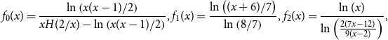 \begin{align*} f_0(x)=\frac {\ln \left (x(x-1)/2\right )}{xH(2/x)-\ln \left (x(x-1)/2\right )}\textrm {, } f_1(x)=\frac {\ln \big ((x+6)/7\big )}{\ln \left (8/7\right )}\textrm {, } f_2(x)=\frac {\ln (x)}{\ln \left (\frac {2(7x-12)}{9(x-2)}\right )}\textrm {,} \end{align*}
i.e. $d^*=f_0(k)+1$
,
$d^*=f_0(k)+1$
, $d_{\bar x}=f_1(k)+1$
and
$d_{\bar x}=f_1(k)+1$
and $d_k=f_2(k)+1$
for all
$d_k=f_2(k)+1$
for all $k\in \mathbb {Z}_{\ge 4}$
. We start with the asymptotic comparison of
$k\in \mathbb {Z}_{\ge 4}$
. We start with the asymptotic comparison of $f_1$
and
$f_1$
and $f_2$
. The corresponding rearrangement gives
$f_2$
. The corresponding rearrangement gives
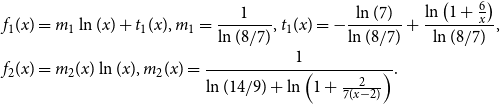 \begin{align*} f_1(x)&=m_1\ln (x)+t_1(x)\textrm {, }m_1=\frac {1}{\ln (8/7)}\textrm {, }t_1(x)=-\frac {\ln (7)}{\ln (8/7)}+\frac {\ln \left (1+\frac {6}{x}\right )}{\ln (8/7)}\textrm {,}\\ f_2(x)&=m_2(x)\ln (x)\textrm {, }m_2(x)=\frac {1}{\ln (14/9)+\ln \left (1+\frac {2}{7(x-2)}\right )}\textrm {.} \end{align*}
Notice that $\ln (x)\gt 0$
since
$\ln (x)\gt 0$
since $x\ge 3$
, further
$x\ge 3$
, further $t_1(x)$
is decreasing while
$t_1(x)$
is decreasing while $m_2(x)$
is increasing, and thereby we have
$m_2(x)$
is increasing, and thereby we have $f_1(x)\ge f_{1\infty }(x)$
and
$f_1(x)\ge f_{1\infty }(x)$
and $f_2(x)\le f_{2\infty }(x)$
with
$f_2(x)\le f_{2\infty }(x)$
with
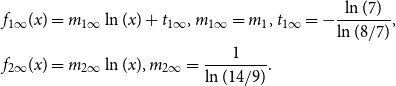 \begin{align*} f_{1\infty }(x) &=m_{1\infty }\ln (x)+t_{1\infty }\textrm {, }m_{1\infty }=m_1\textrm {, }t_{1\infty }=-\frac {\ln (7)}{\ln (8/7)}\textrm {,}\\ f_{2\infty }(x) &=m_{2\infty }\ln (x)\textrm {, }m_{2\infty }=\frac {1}{\ln (14/9)}\textrm {.} \end{align*}
Notice that $m_{1\infty }\gt m_{2\infty }$
,
$m_{1\infty }\gt m_{2\infty }$
, $t_{1\infty }\lt 0$
and further
$t_{1\infty }\lt 0$
and further $f_{1\infty }(x)\gt f_{2\infty }(x)$
iff
$f_{1\infty }(x)\gt f_{2\infty }(x)$
iff $x\gt x_{12}$
with
$x\gt x_{12}$
with $x_{12}=\exp \left (\frac {-t_{1\infty }}{m_{1\infty }-m_{2\infty }}\right )\in (16,17)$
, so
$x_{12}=\exp \left (\frac {-t_{1\infty }}{m_{1\infty }-m_{2\infty }}\right )\in (16,17)$
, so $f_1(x)\gt f_2(x)$
for all
$f_1(x)\gt f_2(x)$
for all $x\in \mathbb {R}_{\ge 17}$
and hence
$x\in \mathbb {R}_{\ge 17}$
and hence $d_k\lt d_{\bar x}$
for
$d_k\lt d_{\bar x}$
for $k\in \mathbb {Z}_{\ge 17}$
. We check by hand that
$k\in \mathbb {Z}_{\ge 17}$
. We check by hand that $d_k\lt d_{\bar x}$
also holds for
$d_k\lt d_{\bar x}$
also holds for $4\le k\le 16$
.
$4\le k\le 16$
.
We are left to show that $1\lt f_0(x)\lt f_2(x)$
for
$1\lt f_0(x)\lt f_2(x)$
for $x\in \mathbb {Z}_{\ge 4}$
. Again, we start with the asymptotic comparison, where the corresponding rearrangement
$x\in \mathbb {Z}_{\ge 4}$
. Again, we start with the asymptotic comparison, where the corresponding rearrangement $f_0(x)=m_0(x)\ln (x)+t_0(x)$
is given by
$f_0(x)=m_0(x)\ln (x)+t_0(x)$
is given by
 \begin{align*} m_0(x)&=\frac {1+\ln \left (1-\frac {1}{x}\right )}{n_0(x)}\textrm {,}\,\, t_0(x)=\frac {-\ln (2)}{n_0(x)}\textrm {,}\,\, n_0(x) =-(x-2)\ln \left (1-\frac {2}{x}\right )-\ln \left (1-\frac {1}{x}\right )-\ln (2)\textrm {.} \end{align*}
Recall that for given $c\in \mathbb {R}$
we have
$c\in \mathbb {R}$
we have $\ln (1+\frac {c}{x})\sim \frac {c}{x}$
and
$\ln (1+\frac {c}{x})\sim \frac {c}{x}$
and $\ln (1+\frac {c}{x})\le \frac {c}{x}$
for all
$\ln (1+\frac {c}{x})\le \frac {c}{x}$
for all $x\in \mathbb {R}_{\gt |c|}$
, since
$x\in \mathbb {R}_{\gt |c|}$
, since $\ln (x)$
is concave and the tangent at
$\ln (x)$
is concave and the tangent at $1$
is
$1$
is $x-1$
. Hence, for all
$x-1$
. Hence, for all $x\in \mathbb {R}_{\ge 3}$
we have
$x\in \mathbb {R}_{\ge 3}$
we have $n_0(x)\ge n_+(x)\gt 0$
since
$n_0(x)\ge n_+(x)\gt 0$
since $x\gt 2$
and
$x\gt 2$
and $x\gt x_1$
, where
$x\gt x_1$
, where
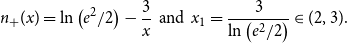 \begin{align*} n_+(x)=\ln \left ({e^2}/{2}\right )-\frac {3}{x} \,\, \textrm {and} \,\, x_1=\frac {3}{\ln \left ({e^2}/{2}\right )}\in (2,3)\textrm {.} \end{align*}
Since $t_0(x)\lt 0$
and
$t_0(x)\lt 0$
and $m_0(x)\le m_+(x)$
we have
$m_0(x)\le m_+(x)$
we have $f_0(x)\le f_+(x)=m_+(x)\ln (x)$
with
$f_0(x)\le f_+(x)=m_+(x)\ln (x)$
with
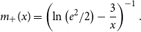 \begin{align*} m_+(x) = \left ( \ln \left ({e^2}/{2}\right )-\frac {3}{x} \right )^{-1}\textrm {.} \end{align*}
Now, since $m_+(x)$
is decreasing in
$m_+(x)$
is decreasing in $x$
and
$x$
and $m_2(x)$
is increasing in
$m_2(x)$
is increasing in $x$
, we numerically determine
$x$
, we numerically determine $x^*\in \mathbb {R}_{\gt 0}$
such that
$x^*\in \mathbb {R}_{\gt 0}$
such that $m_+(x^*)=m_2(x^*)$
and find that
$m_+(x^*)=m_2(x^*)$
and find that $x^*\in (4,5)$
. In particular, we have
$x^*\in (4,5)$
. In particular, we have $f_0(x)\le f_+(x)\lt f_2(x)$
for
$f_0(x)\le f_+(x)\lt f_2(x)$
for $x\in \mathbb {R}_{\ge 5}$
, and check that
$x\in \mathbb {R}_{\ge 5}$
, and check that $d^*\lt d_k$
for
$d^*\lt d_k$
for $k=4$
by hand.
$k=4$
by hand.
Lemma 5.20 concludes the proof of Proposition 2.5 as discussed before.
The left figure shows a sequence $\gamma =(\gamma _1,\gamma _2)$
of two directed (intersecting) four-cycles with base variables
$\gamma =(\gamma _1,\gamma _2)$
of two directed (intersecting) four-cycles with base variables $i_1$
and
$i_1$
and $i_3$
and directions indicated by the arrows respectively. Analogously to Figure 2a we only denoted the
$i_3$
and directions indicated by the arrows respectively. Analogously to Figure 2a we only denoted the $i$
-edges and
$i$
-edges and $a$
-edges instead of the v-edges and f-edges. The relative positions
$a$
-edges instead of the v-edges and f-edges. The relative positions $\rho =(\rho _1,\rho _2)$
corresponding to
$\rho =(\rho _1,\rho _2)$
corresponding to $\gamma$
are depicted in the right figure. Here, the variables, constraints,
$\gamma$
are depicted in the right figure. Here, the variables, constraints, $i$
-edges and
$i$
-edges and $a$
-edges are labelled according to the order of first traversal (where
$a$
-edges are labelled according to the order of first traversal (where $\gamma _1$
is traversed before
$\gamma _1$
is traversed before $\gamma _2$
). The numbers
$\gamma _2$
). The numbers $n(\rho )=3$
,
$n(\rho )=3$
, $m(\rho )=3$
,
$m(\rho )=3$
, $e(\rho )=7$
of variables, constraints and edges in
$e(\rho )=7$
of variables, constraints and edges in $\rho$
are equal to the corresponding numbers in
$\rho$
are equal to the corresponding numbers in $\gamma$
, further the degree
$\gamma$
, further the degree $d_j(\rho )$
of the variable
$d_j(\rho )$
of the variable $j\in [3]$
equals the degree of
$j\in [3]$
equals the degree of $i_j$
in
$i_j$
in $\gamma$
, and analogously for the degrees
$\gamma$
, and analogously for the degrees $k_b(\rho )$
of the constraints
$k_b(\rho )$
of the constraints $b\in [3]$
in
$b\in [3]$
in $\rho$
. The absolute values
$\rho$
. The absolute values $\alpha =(\alpha _v,\alpha _f,(\alpha _{v,j})_{j\in [3]},(\alpha _{f,b})_{b\in [3]})$
are given by
$\alpha =(\alpha _v,\alpha _f,(\alpha _{v,j})_{j\in [3]},(\alpha _{f,b})_{b\in [3]})$
are given by $\alpha _v=(i_j)_{j\in [3]}$
,
$\alpha _v=(i_j)_{j\in [3]}$
, $\alpha _f=(a_b)_{b\in [3]}$
,
$\alpha _f=(a_b)_{b\in [3]}$
, $\alpha _{v,j}=(h_{i_j,e})_{e\in [d_j(\rho )]}$
,
$\alpha _{v,j}=(h_{i_j,e})_{e\in [d_j(\rho )]}$
, $j\in [3]$
, and
$j\in [3]$
, and $\alpha _{f,b}=(h_{a_b,e})_{e\in [k_b(\rho )]}$
,
$\alpha _{f,b}=(h_{a_b,e})_{e\in [k_b(\rho )]}$
, $b\in [3]$
, i.e. they store the (initial) labels of
$b\in [3]$
, i.e. they store the (initial) labels of $\gamma$
corresponding to the labels of
$\gamma$
corresponding to the labels of $\rho$
.
$\rho$
.

6. Small subgraph conditioning
In this section we prove the remaining parts of Theorem2.7, thereby establishing Theorem2.1. The first part of the proof heavily relies on Section A and illustrates the correspondences. We start with the derivation of $\delta _\ell$
by computing
$\delta _\ell$
by computing $\mathbb {E}[ZX_\ell ]$
. For this purpose we fix
$\mathbb {E}[ZX_\ell ]$
. For this purpose we fix $\ell \in \mathbb {Z}_{\gt 0}$
,
$\ell \in \mathbb {Z}_{\gt 0}$
, $n\in \mathcal N$
sufficiently large, and let
$n\in \mathcal N$
sufficiently large, and let $\bar c_\ell$
denote the canonical
$\bar c_\ell$
denote the canonical $2\ell$
-cycle, i.e. the cycle with variables
$2\ell$
-cycle, i.e. the cycle with variables $i$
, constraints
$i$
, constraints $a$
in
$a$
in $[\ell ]$
and
$[\ell ]$
and $i$
-edges,
$i$
-edges, $a$
-edges in
$a$
-edges in $\{1,2\}$
with labels ordered by first traversal, see e.g. the left cycle in Figure 3b. Analogous to the previous sections we rewrite the expectation and count the number
$\{1,2\}$
with labels ordered by first traversal, see e.g. the left cycle in Figure 3b. Analogous to the previous sections we rewrite the expectation and count the number $|\mathcal{E}|$
of triplets
$|\mathcal{E}|$
of triplets $(g,c,x)\in \mathcal{E}$
such that
$(g,c,x)\in \mathcal{E}$
such that $c$
is a
$c$
is a $2\ell$
-cycle and
$2\ell$
-cycle and $x$
a solution in
$x$
a solution in $g$
, i.e.
$g$
, i.e.
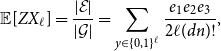 \begin{align*} \mathbb {E}[ZX_\ell ]&=\frac {|\mathcal{E}|}{|\mathcal{G}|} =\sum _{y\in \{0,1\}^\ell }\frac {e_1e_2e_3}{2\ell (dn)!}\textrm {,} \end{align*}
where
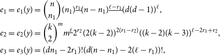 \begin{align*} e_1&=e_1(y)=\binom {n}{n_1}(n_1)^{\underline {r_1}}(n-n_1)^{\underline {\ell -r_1}}(d(d-1))^\ell \textrm {,}\\ e_2&=e_2(y)=\binom {k}{2}^mm^{\underline {\ell }}2^{r_2}(2(k-2))^{2(r_1-r_2)}((k-2)(k-3))^{\ell -2r_1+r_2}\textrm {,}\\ e_3&=e_3(y)=(dn_1-2r_1)!(d(n-n_1)-2(\ell -r_1))!\textrm {,} \end{align*}
and $r=r(y)=(r_1,r_2)$
is defined as follows. For
$r=r(y)=(r_1,r_2)$
is defined as follows. For $y\in \{0,1\}^\ell$
we let
$y\in \{0,1\}^\ell$
we let $r_1=r_1(y)$
denote the number of ones in
$r_1=r_1(y)$
denote the number of ones in $y$
. Further, let
$y$
. Further, let $r_2=r_2(y)$
denote the number of constraints
$r_2=r_2(y)$
denote the number of constraints $b\in [\ell ]$
in
$b\in [\ell ]$
in $\bar c_\ell$
such that both
$\bar c_\ell$
such that both $b$
-edges take the value one under the assignment
$b$
-edges take the value one under the assignment $y$
of the variables
$y$
of the variables $j\in [\ell ]$
in
$j\in [\ell ]$
in $\bar c_\ell$
. With
$\bar c_\ell$
. With $y$
fixed we can compute the number of suitable triplets
$y$
fixed we can compute the number of suitable triplets $(g,c,x)$
as follows. The denominator in the first line reflects
$(g,c,x)$
as follows. The denominator in the first line reflects $|\mathcal{G}|^{-1}$
and the compensation
$|\mathcal{G}|^{-1}$
and the compensation $2\ell$
as we will count directed cycles
$2\ell$
as we will count directed cycles $\gamma$
in
$\gamma$
in $g$
. The sum over
$g$
. The sum over $y\in \{0,1\}^\ell$
implements the choice of the assignment of the variables visited by
$y\in \{0,1\}^\ell$
implements the choice of the assignment of the variables visited by $\gamma$
such that the variables
$\gamma$
such that the variables $i_1,\ldots, i_\ell$
traversed by
$i_1,\ldots, i_\ell$
traversed by $\gamma$
correspond to the variables
$\gamma$
correspond to the variables $1,\ldots, \ell$
in
$1,\ldots, \ell$
in $\bar c_\ell$
in this order, i.e.
$\bar c_\ell$
in this order, i.e. $x_{i_1}=y_1,\ldots, x_{i_\ell }=y_\ell$
. The first term in
$x_{i_1}=y_1,\ldots, x_{i_\ell }=y_\ell$
. The first term in $e_1$
chooses the variables that take the value one under the solution
$e_1$
chooses the variables that take the value one under the solution $x$
. Then we choose the
$x$
. Then we choose the $r_1$
variables out of the
$r_1$
variables out of the $n_1$
-variables that participate in the directed cycle
$n_1$
-variables that participate in the directed cycle $\gamma$
and take the value one consistent with
$\gamma$
and take the value one consistent with $y$
(hence an ordered choice). Analogously, we then choose the variables in
$y$
(hence an ordered choice). Analogously, we then choose the variables in $\gamma$
taking zero under
$\gamma$
taking zero under $x$
. Finally, we choose the two
$x$
. Finally, we choose the two $i$
-edges traversed by
$i$
-edges traversed by $\gamma$
for each of the
$\gamma$
for each of the $\ell$
variables
$\ell$
variables $i$
in the cycle.
$i$
in the cycle.
The first term in $e_2$
is the usual choice of the two
$e_2$
is the usual choice of the two $a$
-edges taking one under
$a$
-edges taking one under $x$
for each
$x$
for each $a\in [m]$
. Then we choose the constraints visited by
$a\in [m]$
. Then we choose the constraints visited by $\gamma$
. The remaining terms account for the ordered choice of the two
$\gamma$
. The remaining terms account for the ordered choice of the two $a$
-edges that are traversed by
$a$
-edges that are traversed by $\gamma$
and that is consistent with the assignments
$\gamma$
and that is consistent with the assignments $y$
and
$y$
and $x$
in the following sense. The (already chosen) variables
$x$
in the following sense. The (already chosen) variables $i_1,\ldots, i_\ell$
and constraints
$i_1,\ldots, i_\ell$
and constraints $a_1,\ldots, a_\ell$
traversed by
$a_1,\ldots, a_\ell$
traversed by $\gamma$
correspond to the variables
$\gamma$
correspond to the variables $1,\ldots, \ell$
and constraints
$1,\ldots, \ell$
and constraints $1,\ldots, \ell$
in
$1,\ldots, \ell$
in $\bar c_\ell$
in this order respectively. Further, the assignment of these variables is already fixed by
$\bar c_\ell$
in this order respectively. Further, the assignment of these variables is already fixed by $y$
and the
$y$
and the $a$
-edges taking the value one for each of these constraints are also fixed by our previous choice. Hence, if
$a$
-edges taking the value one for each of these constraints are also fixed by our previous choice. Hence, if $y_1=y_2=1$
, then we have only two choices for the
$y_1=y_2=1$
, then we have only two choices for the $a_1$
-edge connecting to
$a_1$
-edge connecting to $i_1$
, while the
$i_1$
, while the $a_1$
-edge connecting to
$a_1$
-edge connecting to $i_2$
is fixed afterwards. For
$i_2$
is fixed afterwards. For $y_1=1$
and
$y_1=1$
and $y_2=0$
we have two choices for the
$y_2=0$
we have two choices for the $a_1$
-edge connecting to
$a_1$
-edge connecting to $i_1$
and
$i_1$
and $(k-2)$
choices for the
$(k-2)$
choices for the $a_1$
-edge connecting to
$a_1$
-edge connecting to $i_2$
. The case
$i_2$
. The case $y_1=0$
,
$y_1=0$
, $y_2=1$
is symmetric and we see that we have
$y_2=1$
is symmetric and we see that we have $(k-2)$
and
$(k-2)$
and $(k-3)$
choices for the remaining case
$(k-3)$
choices for the remaining case $y_1=y_2=0$
analogously. To derive the number of constraints for each of the cases above we recall that we have
$y_1=y_2=0$
analogously. To derive the number of constraints for each of the cases above we recall that we have $r_1(y)$
ones in total and
$r_1(y)$
ones in total and $r_2(y)$
ones whose successor is one (i.e. the constraint
$r_2(y)$
ones whose successor is one (i.e. the constraint $a$
between the two ones takes the value one on both
$a$
between the two ones takes the value one on both $a$
-edges, and where the successor of
$a$
-edges, and where the successor of $y_\ell$
is
$y_\ell$
is $y_1$
). But then
$y_1$
). But then $(r_1-r_2)$
ones in
$(r_1-r_2)$
ones in $y$
do not have the successor one, i.e. they have the successor zero. Complementarily we see that since
$y$
do not have the successor one, i.e. they have the successor zero. Complementarily we see that since $r_2$
ones are succeeded by a one there are
$r_2$
ones are succeeded by a one there are $r_2$
ones that are preceded by a one, hence there are
$r_2$
ones that are preceded by a one, hence there are $(r_1-r_2)$
ones that are preceded by zero. Then again, this means that there are
$(r_1-r_2)$
ones that are preceded by zero. Then again, this means that there are $(r_1-r_2)$
zeros that are succeeded by a one, hence the remaining
$(r_1-r_2)$
zeros that are succeeded by a one, hence the remaining $(\ell -2r_1+r_2)$
zeros out of the
$(\ell -2r_1+r_2)$
zeros out of the $(\ell -r_1)$
zeros are succeeded by a zero. This fixes
$(\ell -r_1)$
zeros are succeeded by a zero. This fixes $\gamma$
, so in particular
$\gamma$
, so in particular $2r_1$
v-edges that take the value one and
$2r_1$
v-edges that take the value one and $2(\ell -r_1)$
v-edges that take the value zero. The two terms in
$2(\ell -r_1)$
v-edges that take the value zero. The two terms in $e_3$
then wire the remaining edges.
$e_3$
then wire the remaining edges.
We divide by $\mathbb {E}[Z]$
to match the left hand side of Theorem2.7b), i.e.
$\mathbb {E}[Z]$
to match the left hand side of Theorem2.7b), i.e.
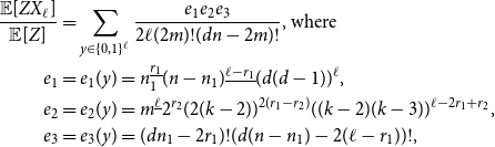 \begin{align*} \frac {\mathbb {E}[ZX_\ell ]}{\mathbb {E}[Z]} &=\sum _{y\in \{0,1\}^\ell }\frac {e_1e_2e_3}{2\ell (2m)!(dn-2m)!}\textrm {, where}\\ e_1&=e_1(y)=n_1^{\underline {r_1}}(n-n_1)^{\underline {\ell -r_1}}(d(d-1))^\ell \textrm {,}\\ e_2&=e_2(y)=m^{\underline {\ell }}2^{r_2}(2(k-2))^{2(r_1-r_2)}((k-2)(k-3))^{\ell -2r_1+r_2}\textrm {,}\\ e_3&=e_3(y)=(dn_1-2r_1)!(d(n-n_1)-2(\ell -r_1))!\textrm {,} \end{align*}
and using Stirling’s formula we easily derive that
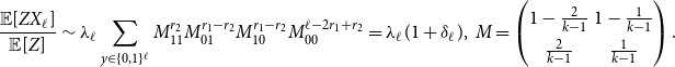 \begin{align*} \frac {\mathbb {E}[ZX_\ell ]}{\mathbb {E}[Z]}&\sim \lambda _\ell \sum _{y\in \{0,1\}^\ell } M_{11}^{r_2}M_{01}^{r_1-r_2}M_{10}^{r_1-r_2}M_{00}^{\ell -2r_1+r_2} =\lambda _\ell (1+\delta _\ell )\textrm {, }\, M=\begin{pmatrix} 1-\frac {2}{k-1} & 1-\frac {1}{k-1}\\ \frac {2}{k-1} & \frac {1}{k-1} \end{pmatrix}\textrm {.} \end{align*}
The matrix $M$
has a nice interpretation as a (column stochastic) transition probability matrix in a two state Markov process, with
$M$
has a nice interpretation as a (column stochastic) transition probability matrix in a two state Markov process, with
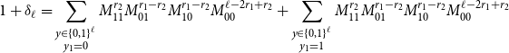 \begin{align*} 1+\delta _\ell =\sum _{\substack {y\in \{0,1\}^\ell \\y_1=0}}M_{11}^{r_2}M_{01}^{r_1-r_2}M_{10}^{r_1-r_2}M_{00}^{\ell -2r_1+r_2} +\sum _{\substack {y\in \{0,1\}^\ell \\y_1=1}}M_{11}^{r_2}M_{01}^{r_1-r_2}M_{10}^{r_1-r_2}M_{00}^{\ell -2r_1+r_2} \end{align*}
reflecting the probabilities that we return to the starting point given that the starting point is zero and one respectively. Let us consider the first partial sum restricted to sequences $y$
(of Markov states) such that
$y$
(of Markov states) such that $y_1=0$
, i.e. we start in the state zero. Then
$y_1=0$
, i.e. we start in the state zero. Then $M_{0y_2}$
reflects the probability that we move from the initial state zero to the state
$M_{0y_2}$
reflects the probability that we move from the initial state zero to the state $y_2$
given that we are in state zero (which is the case because we know that
$y_2$
given that we are in state zero (which is the case because we know that $y_1=0$
). As discussed above we will move from a one to a one in
$y_1=0$
). As discussed above we will move from a one to a one in $y$
exactly
$y$
exactly $r_2$
times, from a one to a zero
$r_2$
times, from a one to a zero $(r_1-r_2)$
times, from a zero to a one
$(r_1-r_2)$
times, from a zero to a one $(r_1-r_2)$
times and from a zero to a zero
$(r_1-r_2)$
times and from a zero to a zero $(\ell -2r_1+r_2)$
times. Hence the contribution to the first partial sum for given
$(\ell -2r_1+r_2)$
times. Hence the contribution to the first partial sum for given $y$
exactly reflects the probability that we start in the state zero and (with this given) return to the state zero after
$y$
exactly reflects the probability that we start in the state zero and (with this given) return to the state zero after $\ell$
steps (since the successor of
$\ell$
steps (since the successor of $y_\ell$
is
$y_\ell$
is $y_1=0$
). Since we sum over all such sequences
$y_1=0$
). Since we sum over all such sequences $y$
the first sum reflects the probability that we reach state zero after
$y$
the first sum reflects the probability that we reach state zero after $\ell$
steps given that we start in the state zero. The discussion of the second sum is completely analogous. This directly yields
$\ell$
steps given that we start in the state zero. The discussion of the second sum is completely analogous. This directly yields
 \begin{align*} 1+\delta _\ell =(M^\ell )_{00}+(M^\ell )_{11}=\textrm {Tr}(M^\ell )=\lambda ^{\prime}_1+\lambda ^{\prime}_2=\lambda _1^\ell +\lambda _2^\ell \textrm {, } \quad \lambda _1=1\textrm {, } \lambda _2=-\frac {1}{k-1}\textrm {,} \end{align*}
where we used the Kolmogorov-Chapman equalities in the first step, i.e. that the $\ell$
-step transition probability matrix is the
$\ell$
-step transition probability matrix is the $\ell$
-th power of the one step transition probability matrix, which allow to translate the first sum into the transition probability
$\ell$
-th power of the one step transition probability matrix, which allow to translate the first sum into the transition probability $(M^\ell )_{00}$
that we reach the state zero after
$(M^\ell )_{00}$
that we reach the state zero after $\ell$
steps given that we start in the state zero and analogously for the second sum. In the second step we use the definition of the trace, while in the third step we use that the trace is the sum of the eigenvalues
$\ell$
steps given that we start in the state zero and analogously for the second sum. In the second step we use the definition of the trace, while in the third step we use that the trace is the sum of the eigenvalues $\lambda ^{\prime}_1$
,
$\lambda ^{\prime}_1$
, $\lambda ^{\prime}_2$
of
$\lambda ^{\prime}_2$
of $M^\ell$
. In the next step we use that the eigenvalues
$M^\ell$
. In the next step we use that the eigenvalues $\lambda ^{\prime}_1$ $\lambda ^{\prime}_2$
of the
$\lambda ^{\prime}_2$
of the $\ell$
-th power
$\ell$
-th power $M^\ell$
of the matrix
$M^\ell$
of the matrix $M$
are the
$M$
are the $\ell$
-th powers of the eigenvalues
$\ell$
-th powers of the eigenvalues $\lambda _1$
,
$\lambda _1$
, $\lambda _2$
of
$\lambda _2$
of $M$
. In particular this also yields that
$M$
. In particular this also yields that $\delta _\ell \gt -1$
for all
$\delta _\ell \gt -1$
for all $k\gt 3$
and establishes
$k\gt 3$
and establishes $\delta _\ell =(1-k)^{-\ell }$
.
$\delta _\ell =(1-k)^{-\ell }$
.
Following the strategy of Section A we turn to the case of disjoint cycles. Similarly, the present case is a canonical extension of the single cycle case discussed above. We fix $L\in \mathbb {Z}_{\gt 0}$
,
$L\in \mathbb {Z}_{\gt 0}$
, $r\in \mathbb {Z}_{\ge 0}^{L}$
and
$r\in \mathbb {Z}_{\ge 0}^{L}$
and $n\in \mathcal N$
sufficiently large. Further, as in the previous sections we rewrite the expectation and count the number
$n\in \mathcal N$
sufficiently large. Further, as in the previous sections we rewrite the expectation and count the number $|\mathcal{E}|$
of triplets
$|\mathcal{E}|$
of triplets $(g,c,x)\in \mathcal{E}$
such that
$(g,c,x)\in \mathcal{E}$
such that $c=(c_s)_{s\in [\bar r]}$
is a sequence of
$c=(c_s)_{s\in [\bar r]}$
is a sequence of $\bar r=\sum _{\ell \in [L]}r_\ell$
distinct
$\bar r=\sum _{\ell \in [L]}r_\ell$
distinct $2\ell _s$
-cycles
$2\ell _s$
-cycles $c_s$
in the configuration
$c_s$
in the configuration $g$
sorted by their length
$g$
sorted by their length $\ell _s$
in ascending order (as described in Section A) and
$\ell _s$
in ascending order (as described in Section A) and $x$
is a solution of
$x$
is a solution of $g$
. This yields
$g$
. This yields
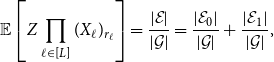 \begin{align*} \mathbb {E}\left [Z\prod _{\ell \in [L]}(X_\ell )_{r_\ell }\right ]=\frac {|\mathcal{E}|}{|\mathcal{G}|} =\frac {|\mathcal{E}_0|}{|\mathcal{G}|}+\frac {|\mathcal{E}_1|}{|\mathcal{G}|}\textrm {,} \end{align*}
where $\mathcal{E}_0\subseteq \mathcal{E}$
is the set over all triplets
$\mathcal{E}_0\subseteq \mathcal{E}$
is the set over all triplets $(g,c,x)\in \mathcal{E}$
involving sequences
$(g,c,x)\in \mathcal{E}$
involving sequences $c$
of disjoint cycles and
$c$
of disjoint cycles and $\mathcal{E}_1=\mathcal{E}\setminus \mathcal{E}_0$
. We begin with the first contribution, which can be regarded as a combination of the discussion of disjoint cycles in Section A and the single cycle case above, i.e.
$\mathcal{E}_1=\mathcal{E}\setminus \mathcal{E}_0$
. We begin with the first contribution, which can be regarded as a combination of the discussion of disjoint cycles in Section A and the single cycle case above, i.e.
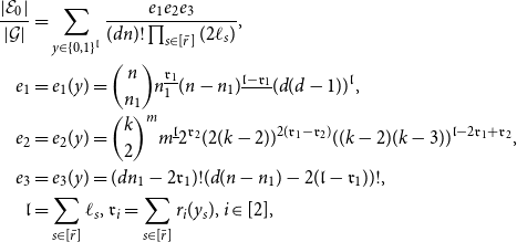 \begin{align*} \frac {|\mathcal{E}_0|}{|\mathcal{G}|}&=\sum _{y\in \{0,1\}^{\mathfrak l}}\frac {e_1e_2e_3}{(dn)!\prod _{s\in [\bar r]}(2\ell _s)}\textrm {,}\\ e_1&=e_1(y)=\binom {n}{n_1}n_1^{\underline {\mathfrak r_1}}(n-n_1)^{\underline {\mathfrak l-\mathfrak r_1}}(d(d-1))^{\mathfrak l}\textrm {,}\\ e_2&=e_2(y)=\binom {k}{2}^mm^{\underline {\mathfrak l}}2^{\mathfrak r_2}(2(k-2))^{2(\mathfrak r_1-\mathfrak r_2)}((k-2)(k-3))^{\mathfrak l-2\mathfrak r_1+\mathfrak r_2}\textrm {,}\\ e_3&=e_3(y)=(dn_1-2\mathfrak r_1)!(d(n-n_1)-2(\mathfrak l-\mathfrak r_1))!\textrm {,}\\ \mathfrak l&=\sum _{s\in [\bar r]}\ell _s\textrm {, } \mathfrak r_i=\sum _{s\in [\bar r]}r_i(y_s)\textrm {, }i\in [2]\textrm {,} \end{align*}
where $y=(y_s)_{s\in [\bar r]}$
is the subdivision of
$y=(y_s)_{s\in [\bar r]}$
is the subdivision of $y$
corresponding to the definition of
$y$
corresponding to the definition of $c$
, and
$c$
, and $r_1$
,
$r_1$
, $r_2$
are the notions defined above. The combinatorial arguments are now fairly self-explanatory, e.g. we make an ordered choice of the
$r_2$
are the notions defined above. The combinatorial arguments are now fairly self-explanatory, e.g. we make an ordered choice of the $r_1(y_1)$
variables taking one for
$r_1(y_1)$
variables taking one for $\gamma _1$
, then an ordered choice of
$\gamma _1$
, then an ordered choice of $r_1(y_2)$
variables taking one for
$r_1(y_2)$
variables taking one for $\gamma _2$
out of the remaining
$\gamma _2$
out of the remaining $n_1-r_1(y_1)$
variables taking one and so on.
$n_1-r_1(y_1)$
variables taking one and so on.
The asymptotics are also completely analogous to the single cycle case and Section A. First, we notice that the sum is still bounded, i.e. we can also use the asymptotic equivalences for the corresponding ratio here. Then, the sum can be decomposed into the product of the $\bar r$
factors that correspond to the single cycle case above, analogously to Section A, which yields
$\bar r$
factors that correspond to the single cycle case above, analogously to Section A, which yields
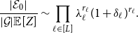 \begin{align*} \frac {|\mathcal{E}_0|}{|\mathcal{G}|\mathbb {E}[Z]}\sim \prod _{\ell \in [L]}\lambda _\ell ^{r_\ell }(1+\delta _\ell )^{r_\ell }\textrm {.} \end{align*}
Now we turn to the proof that the second contribution involving $\mathcal{E}_1$
is negligible, which is a combination of the above and the discussion of intersecting cycles in Section A. We let
$\mathcal{E}_1$
is negligible, which is a combination of the above and the discussion of intersecting cycles in Section A. We let
 \begin{align*} \mathcal{E}_2&=\{(g,\gamma, x)\,:\,(g,c(\gamma ),x)\in \mathcal{E}_1\}\textrm {, } \mathcal R=\{\rho (\gamma )\,:\,(g,\gamma, x)\in \mathcal{E}_2\}\textrm { and }\\ \mathcal{E}_{\rho }&=\{(g,\gamma, x)\in \mathcal{E}_2\,:\,\rho (\gamma )=\rho \}\textrm { for }\rho \in \mathcal R \end{align*}
denote the sets that match the corresponding sets in Section A. For relative positions $\rho \in \mathcal R$
we consider an assignment
$\rho \in \mathcal R$
we consider an assignment $y\in \{0,1\}^{n(\rho )}$
of the variables
$y\in \{0,1\}^{n(\rho )}$
of the variables $V=[n(\rho )]$
in the corresponding union of cycles
$V=[n(\rho )]$
in the corresponding union of cycles $c=c(\rho )$
and let
$c=c(\rho )$
and let
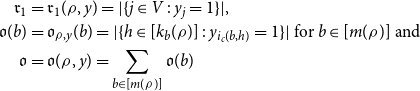 \begin{align*} \mathfrak r_1&=\mathfrak r_1(\rho, y)=|\{j\in V\,:\,y_j=1\}|\textrm {,}\\ \mathfrak o(b)&=\mathfrak o_{\rho, y}(b)=|\{h\in [k_b(\rho )]\,:\,y_{i_c(b,h)}=1\}|\textrm { for }b\in [m(\rho )]\textrm { and}\\ \mathfrak o&=\mathfrak o(\rho, y)=\sum _{b\in [m(\rho )]}\mathfrak o(b) \end{align*}
denote the number of variables $j\in V$
in
$j\in V$
in $c$
that take the value one under
$c$
that take the value one under $y$
, the number of
$y$
, the number of $b$
-edges for a constraint
$b$
-edges for a constraint $b\in [m(\rho )]$
in
$b\in [m(\rho )]$
in $c$
that take the value one under
$c$
that take the value one under $y$
and the number of f-edges in
$y$
and the number of f-edges in $c$
that take the value one under
$c$
that take the value one under $y$
respectively. Since
$y$
respectively. Since $c$
is a configuration the number of v-edges in
$c$
is a configuration the number of v-edges in $c$
that take the value one under
$c$
that take the value one under $y$
is also
$y$
is also $\mathfrak o$
. We are particularly interested in the assignments
$\mathfrak o$
. We are particularly interested in the assignments
 \begin{align*} y\in \mathcal Y=\mathcal Y(\rho )=\{z\in \{0,1\}^{n(\rho )}\,:\,\forall b\in [m(\rho )]\mathfrak o(b)\in [2+k_b-k,2]\} \end{align*}
that do not directly violate a constraint $b\in [m(\rho )]$
in
$b\in [m(\rho )]$
in $c(\rho )$
in the sense that
$c(\rho )$
in the sense that $\mathfrak o(b)\le 2$
and also do not indirectly violate
$\mathfrak o(b)\le 2$
and also do not indirectly violate $b$
in that
$b$
in that $2-\mathfrak o(b)\le k-k_b$
, i.e. there are sufficiently many
$2-\mathfrak o(b)\le k-k_b$
, i.e. there are sufficiently many $b$
-edges left to take the remaining
$b$
-edges left to take the remaining $(2-\mathfrak o(b))$
ones. With this slight extension of our machinery we can derive
$(2-\mathfrak o(b))$
ones. With this slight extension of our machinery we can derive
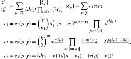 \begin{align*} \frac {|\mathcal{E}_1|}{|\mathcal{G}|} &=\sum _{\rho \in \mathcal R}\frac {|\mathcal{E}_{\rho }|}{(dn)!\prod _{s\in [\mathfrak r]}(2\ell _s)}\textrm {, } |\mathcal{E}_{\rho }| =\sum _{y\in \mathcal Y}e_1e_2e_3\textrm {, }\\ e_1&=e_1(\rho, y) =\binom {n}{n_1}n_1^{\underline {\mathfrak r_1}}(n-n_1)^{\underline {n(\rho )-\mathfrak r_1}}\prod _{j\in [n(\rho )]}d^{\underline {d_j(\rho )}}\textrm {,}\\ e_2&=e_2(\rho, y)=\binom {k}{2}^mm^{\underline {m(\rho )}}\prod _{b\in [m(\rho )]}(2^{\underline {\mathfrak o(b)}}(k-2)^{\underline {k_b(\rho )-\mathfrak o(b)}}) \textrm {,}\\ e_3&=e_3(\rho, y)=(dn_1-\mathfrak o)!(d(n-n_1)-(e(\rho )-\mathfrak o))!\textrm {,} \end{align*}
for the following reasons. With $\rho \in \mathcal R$
and
$\rho \in \mathcal R$
and $y\in \mathcal Y(\rho )$
fixed we choose the
$y\in \mathcal Y(\rho )$
fixed we choose the $n_1$
variables out of the
$n_1$
variables out of the $n$
variables in the configuration
$n$
variables in the configuration $g$
that should take the value one under
$g$
that should take the value one under $x$
. Out of these
$x$
. Out of these $n_1$
variables we choose the
$n_1$
variables we choose the $\mathfrak r_1$
variables (ordered by first traversal) that take the value one in the directed cycles
$\mathfrak r_1$
variables (ordered by first traversal) that take the value one in the directed cycles $\gamma$
under
$\gamma$
under $x$
, corresponding to the
$x$
, corresponding to the $\mathfrak r_1$
variables in
$\mathfrak r_1$
variables in $\rho$
that take one under
$\rho$
that take one under $y$
(more precisely we choose the values
$y$
(more precisely we choose the values $i\in [n]$
of the absolute values
$i\in [n]$
of the absolute values $\alpha _v$
for the
$\alpha _v$
for the $\mathfrak r_1$
variables
$\mathfrak r_1$
variables $j\in [n(\rho )]$
in
$j\in [n(\rho )]$
in $\rho$
that take the value one under
$\rho$
that take the value one under $y$
) and analogously for the variables that take zero. Then, for each variable
$y$
) and analogously for the variables that take zero. Then, for each variable $j\in [n(\rho )]$
in
$j\in [n(\rho )]$
in $\rho$
and corresponding variable
$\rho$
and corresponding variable $i=\alpha _v(j)$
in
$i=\alpha _v(j)$
in $\gamma$
we choose the
$\gamma$
we choose the $i$
-edges that participate in
$i$
-edges that participate in $\gamma$
(meaning that we choose
$\gamma$
(meaning that we choose $\alpha _{v,j}$
). On the constraint side we first choose the two
$\alpha _{v,j}$
). On the constraint side we first choose the two $a$
-edges that take the value one under
$a$
-edges that take the value one under $x$
in
$x$
in $g$
for each
$g$
for each $a\in [m]$
. Then we select the
$a\in [m]$
. Then we select the $m(\rho )$
constraints that participate in
$m(\rho )$
constraints that participate in $\gamma$
(i.e. we fix
$\gamma$
(i.e. we fix $\alpha _f$
). Further, for each constraint
$\alpha _f$
). Further, for each constraint $b\in [m(\rho )]$
in
$b\in [m(\rho )]$
in $\rho$
and its corresponding constraint
$\rho$
and its corresponding constraint $a=\alpha _f(b)$
in
$a=\alpha _f(b)$
in $\gamma$
we choose the
$\gamma$
we choose the $\mathfrak o(b)$ $a$
-edges that take the value one in
$a$
-edges that take the value one in $\gamma$
under
$\gamma$
under $x$
consistent with
$x$
consistent with $\rho$
and
$\rho$
and $y$
out of the two
$y$
out of the two $a$
-edges that take the value one in
$a$
-edges that take the value one in $g$
under
$g$
under $x$
and analogously for the
$x$
and analogously for the $a$
-edges that take the value zero (which means that we fix
$a$
-edges that take the value zero (which means that we fix $\alpha _{f,b}$
for
$\alpha _{f,b}$
for $b\in [m(\rho )]$
consistent with the choice of
$b\in [m(\rho )]$
consistent with the choice of $y$
and the choice of the two
$y$
and the choice of the two $a$
-edges that take the value one for each
$a$
-edges that take the value one for each $a\in [m]$
). This fixes the sequence of the directed cycles (i.e. the isomorphism
$a\in [m]$
). This fixes the sequence of the directed cycles (i.e. the isomorphism $\alpha$
and further
$\alpha$
and further $\gamma$
). The remaining terms wire the
$\gamma$
). The remaining terms wire the $(dn_1-\mathfrak o)$
remaining v-edges that take the value one and the v-edges taking zero respectively.
$(dn_1-\mathfrak o)$
remaining v-edges that take the value one and the v-edges taking zero respectively.
As opposed to the rather demanding combinatorial part the asymptotics are still easy to derive since both sums are bounded, so the procedure analogous to Section A yields
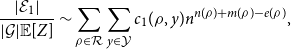 \begin{align*} \frac {|\mathcal{E}_1|}{|\mathcal{G}|\mathbb {E}[Z]} &\sim \sum _{\rho \in \mathcal R}\sum _{y\in \mathcal Y}c_1(\rho, y)n^{n(\rho )+m(\rho )-e(\rho )}\textrm {,} \end{align*}
where $c_1(\rho, y)$
is a constant compensating the bounded terms. The right hand side tends to zero by the argumentation in Section A, so this contribution is indeed negligible. This shows that
$c_1(\rho, y)$
is a constant compensating the bounded terms. The right hand side tends to zero by the argumentation in Section A, so this contribution is indeed negligible. This shows that $\frac {|\mathcal{E}|}{|\mathcal{G}|}\sim \frac {|\mathcal{E}_0|}{|\mathcal{G}|}$
and thereby establishes Theorem2.7 (2).
$\frac {|\mathcal{E}|}{|\mathcal{G}|}\sim \frac {|\mathcal{E}_0|}{|\mathcal{G}|}$
and thereby establishes Theorem2.7 (2).
With $d\in [1,d^*)\subseteq [1,k)$
as discussed in Lemma 5.17 and Lemma 5.20,
$d\in [1,d^*)\subseteq [1,k)$
as discussed in Lemma 5.17 and Lemma 5.20, $\lambda _\ell$
as derived in Lemma 2.8,
$\lambda _\ell$
as derived in Lemma 2.8, $\delta _\ell =(1-k)^{-\ell }$
, the asymptotics of the second moment discussed in Lemma 2.6 and the Taylor series
$\delta _\ell =(1-k)^{-\ell }$
, the asymptotics of the second moment discussed in Lemma 2.6 and the Taylor series $\ln (1-x)= - \sum _{\ell \ge 1} {x^\ell }/{\ell }, x\in (0,1)$
, we establish Theorem2.7 (3) by applying our results to the sum
$\ln (1-x)= - \sum _{\ell \ge 1} {x^\ell }/{\ell }, x\in (0,1)$
, we establish Theorem2.7 (3) by applying our results to the sum
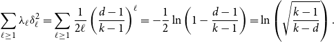 \begin{align*} \sum _{\ell \ge 1}\lambda _\ell \delta _\ell ^2=\sum _{\ell \ge 1}\frac {1}{2\ell }\left (\frac {d-1}{k-1}\right )^\ell =-\frac {1}{2}\ln \left (1-\frac {d-1}{k-1}\right ) =\ln \left (\sqrt {\frac {k-1}{k-d}}\right )\textrm {.} \end{align*}
This concludes the proof of Theorem2.7 and further the proof of Theorem1.1.
Acknowledgements
An extended abstract of a preliminary version of this paper has appeared at the proceedings of ICALP ’19 [36]. The results here apply to all 2-in- $k$
occupation problems, as opposed to only
$k$
occupation problems, as opposed to only $k = 4$
in [36].
$k = 4$
in [36].
Funding statement
The research leading to these results has received funding from the European Research Council, ERC Grant Agreement 772606–PTRCSP.
Appendix
A. Proof of Lemma 2.8
We present the proof of Lemma 2.8 in detail so as to facilitate the presentation of the small subgraph conditioning method in Section 6. Lemma 2.8 can be shown by a direct application of the method of moments, which is discussed, for example, in [Reference Janson, Łuczak and Rucinski24] (Theorem 6.10).
Theorem A.1 (Method of Moments). Let $L\in \mathbb {Z}_{\gt 0}$
and
$L\in \mathbb {Z}_{\gt 0}$
and $((X_{\ell, i})_{\ell \in [L]})_{i\in \mathbb {Z}_{\gt 0}}$
be a sequence of a vector of random variables. If
$((X_{\ell, i})_{\ell \in [L]})_{i\in \mathbb {Z}_{\gt 0}}$
be a sequence of a vector of random variables. If $\lambda \in \mathbb {R}_{\ge 0}^{L}$
is such that, as
$\lambda \in \mathbb {R}_{\ge 0}^{L}$
is such that, as $i\rightarrow \infty$
,
$i\rightarrow \infty$
,
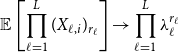 \begin{align*} \mathbb {E}\left [\prod _{\ell =1}^{L}(X_{\ell, i})_{r_\ell }\right ]\rightarrow \prod _{\ell =1}^{L}\lambda _\ell ^{r_\ell } \end{align*}
for every $r\in \mathbb {Z}_{\ge 0}^{L}$
, then
$r\in \mathbb {Z}_{\ge 0}^{L}$
, then $(X_{\ell, i})_{\ell \in [L]}$
converges in distribution to
$(X_{\ell, i})_{\ell \in [L]}$
converges in distribution to $(Z_\ell )_{\ell \in [L]}$
, where the
$(Z_\ell )_{\ell \in [L]}$
, where the $Z_\ell \sim \textrm {Po}(\lambda _\ell )$
are independent Poisson distributed random variables.
$Z_\ell \sim \textrm {Po}(\lambda _\ell )$
are independent Poisson distributed random variables.
First, we notice that $G=G_{k,d,n,m}$
and further
$G=G_{k,d,n,m}$
and further $X_\ell =X_{k,d,n,\ell }$
is only defined for
$X_\ell =X_{k,d,n,\ell }$
is only defined for $m=dn/k\in \mathbb {Z}$
as stated in Lemma 3.1, hence Lemma 2.8 only applies to such sequences of configurations. Fix
$m=dn/k\in \mathbb {Z}$
as stated in Lemma 3.1, hence Lemma 2.8 only applies to such sequences of configurations. Fix $k$
,
$k$
, $d\in \mathbb {Z}_{\gt 1}$
. Before we turn to the general case we consider the
$d\in \mathbb {Z}_{\gt 1}$
. Before we turn to the general case we consider the $\mathbb {E}[X_\ell ]$
for
$\mathbb {E}[X_\ell ]$
for $\ell \in \mathbb {Z}_{\gt 0}$
. For this purpose let
$\ell \in \mathbb {Z}_{\gt 0}$
. For this purpose let $n$
and
$n$
and $m(n)$
be sufficiently large. Let
$m(n)$
be sufficiently large. Let $\mathcal C_{\ell, g}$
be the set of all
$\mathcal C_{\ell, g}$
be the set of all $2\ell$
-cycles in
$2\ell$
-cycles in $g\in \mathcal{G}$
. Then
$g\in \mathcal{G}$
. Then
 \begin{align*} \mathbb {E}[X_\ell ]&=\sum _{g\in \mathcal{G}}\frac {X_\ell (g)}{|\mathcal{G}|} =|\mathcal{G}|^{-1}\sum _{g\in \mathcal{G}}|\mathcal C_{\ell, g}| =\frac {|\mathcal{E}|}{|\mathcal{G}|} \,\textrm {, where } \, \mathcal{E}=\{(g,c):g\in \mathcal{G},c\in \mathcal C_{\ell, g}\}. \end{align*}
With this at hand we obtain that
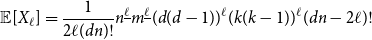 \begin{align*} \mathbb {E}[X_\ell ]=\frac {1}{2\ell (dn)!}n^{\underline {\ell }}m^{\underline {\ell }}(d(d-1))^\ell (k(k-1))^\ell (dn-2\ell )! \end{align*}
using the following combinatorial arguments. Instead of counting pairs $(g,c)$
of configurations
$(g,c)$
of configurations $g$
and
$g$
and $2\ell$
-cycles
$2\ell$
-cycles $c\in \mathcal C_{\ell, g}$
we count pairs
$c\in \mathcal C_{\ell, g}$
we count pairs $(g,\gamma )$
of configurations
$(g,\gamma )$
of configurations $g$
and directed
$g$
and directed $2\ell$
-cycles
$2\ell$
-cycles $\gamma$
(based at a variable node) in
$\gamma$
(based at a variable node) in $g$
. There are exactly
$g$
. There are exactly $2\ell$
directed cycles
$2\ell$
directed cycles $\gamma$
corresponding to each (undirected) cycle
$\gamma$
corresponding to each (undirected) cycle $c$
of length
$c$
of length $2\ell$
since we can choose the base from the
$2\ell$
since we can choose the base from the $\ell$
variables in
$\ell$
variables in $c$
and
$c$
and $\gamma$
is then determined by one of the two possible directions. The denominator reflects the compensation for this counting next to the probability
$\gamma$
is then determined by one of the two possible directions. The denominator reflects the compensation for this counting next to the probability $|\mathcal{G}|^{-1}$
. Further, the term
$|\mathcal{G}|^{-1}$
. Further, the term $n^{\underline {\ell }}$
reflects the ordered choice of the variables for the directed cycle, as does
$n^{\underline {\ell }}$
reflects the ordered choice of the variables for the directed cycle, as does $m^{\underline {\ell }}$
for the constraints. The next two terms account for the choice of the two
$m^{\underline {\ell }}$
for the constraints. The next two terms account for the choice of the two $i$
-edges and
$i$
-edges and $a$
-edges traversed by the cycle for each of the
$a$
-edges traversed by the cycle for each of the $\ell$
variables
$\ell$
variables $i$
and constraints
$i$
and constraints $a$
. This fixes the directed cycle
$a$
. This fixes the directed cycle $\gamma$
and further the corresponding undirected cycle
$\gamma$
and further the corresponding undirected cycle $c(\gamma )$
. In particular, the
$c(\gamma )$
. In particular, the $2\ell$
edges of the cycle
$2\ell$
edges of the cycle $c$
in
$c$
in $g$
are fixed, i.e. the corresponding restriction of
$g$
are fixed, i.e. the corresponding restriction of $g$
to
$g$
to $c$
. This leaves us with
$c$
. This leaves us with $(dn-2\ell )$
half-edges in
$(dn-2\ell )$
half-edges in $\textrm {dom}(g)$
and
$\textrm {dom}(g)$
and $(km-2\ell )$
half-edges in
$(km-2\ell )$
half-edges in $\textrm {im}(g)$
that have not been wired yet. The last term gives the number of such wirings.
$\textrm {im}(g)$
that have not been wired yet. The last term gives the number of such wirings.
Next, we turn to asymptotics. Extracting $\lambda _\ell$
and expanding the falling factorials yields
$\lambda _\ell$
and expanding the falling factorials yields
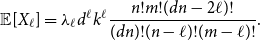 \begin{align*} \mathbb {E}[X_\ell ]=\lambda _\ell d^\ell k^\ell \frac {n!m!(dn-2\ell )!}{(dn)!(n-\ell )!(m-\ell )!}\textrm {.} \end{align*}
Using Stirling’s formula we readily obtain that
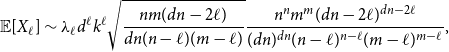 \begin{align*} \mathbb {E}[X_\ell ] &\sim \lambda _\ell d^\ell k^\ell \sqrt {\frac {nm(dn-2\ell )}{dn(n-\ell )(m-\ell )}} \frac {n^nm^m(dn-2\ell )^{dn-2\ell }}{(dn)^{dn}(n-\ell )^{n-\ell }(m-\ell )^{m-\ell }}, \end{align*}
and so
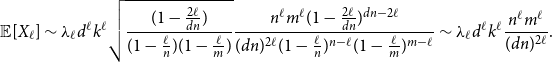 \begin{align*} \mathbb {E}[X_\ell ]&\sim \lambda _\ell d^\ell k^\ell \sqrt {\frac {(1-\frac {2\ell }{dn})}{(1-\frac {\ell }{n})(1-\frac {\ell }{m})}} \frac {n^{\ell }m^{\ell }(1-\frac {2\ell }{dn})^{dn-2\ell }}{(dn)^{2\ell }(1-\frac {\ell }{n})^{n-\ell }(1-\frac {\ell }{m})^{m-\ell }} \sim \lambda _\ell d^\ell k^\ell \frac {n^{\ell }m^{\ell }}{(dn)^{2\ell }}. \end{align*}
Using that $dn = km$
leads to
$dn = km$
leads to
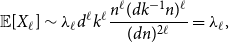 \begin{align*} \mathbb {E}[X_\ell ]&\sim \lambda _\ell d^\ell k^\ell \frac {n^{\ell }(dk^{-1}n)^{\ell }}{(dn)^{2\ell }}=\lambda _\ell \textrm {,} \end{align*}
as claimed. We turn to the general case. For this purpose let $L\in \mathbb {Z}_{\gt 0}$
,
$L\in \mathbb {Z}_{\gt 0}$
, $r\in \mathbb {Z}_{\ge 0}^{L}$
and let
$r\in \mathbb {Z}_{\ge 0}^{L}$
and let $n$
and
$n$
and $m$
be sufficiently large. Then
$m$
be sufficiently large. Then
 \begin{align*} X_\ell (g)^{\underline {r_\ell }}&=\prod _{s=0}^{r_\ell -1}(|\mathcal C_{\ell, g}|-s)=|\mathcal C_{\ell, r_\ell, g}| \,\textrm {, where }\, \mathcal C_{\ell, r_\ell, g} =\{c\in \mathcal C_{\ell, g}^{r_\ell }:\forall s\in [r_\ell ]\forall s^{\prime}\in [s-1]\,c_s\neq c_{s^{\prime}}\} \end{align*}
for $g\in \mathcal{G}$
, since this corresponds to an ordered choice of
$g\in \mathcal{G}$
, since this corresponds to an ordered choice of $2\ell$
-cycles in
$2\ell$
-cycles in $g$
without repetition. The product can then be directly written as
$g$
without repetition. The product can then be directly written as
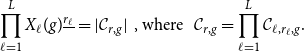 \begin{align*} \prod _{\ell =1}^{L}X_\ell (g)^{\underline {r_\ell }}=|\mathcal C_{r,g}| \,\,\textrm {, where } \,\, \mathcal C_{r,g}=\prod _{\ell =1}^{L}\mathcal C_{\ell, r_\ell, g}\textrm {.} \end{align*}
To avoid double indexed sequences we use the equivalent representation $c=(c_s)_{s\in [\mathfrak r]}\in \mathcal C_{r,g}$
where
$c=(c_s)_{s\in [\mathfrak r]}\in \mathcal C_{r,g}$
where $\mathfrak r=\sum _{1\le \ell \le L} r_\ell$
. From the above we see that the cycles
$\mathfrak r=\sum _{1\le \ell \le L} r_\ell$
. From the above we see that the cycles $c_s$
are ordered by their length
$c_s$
are ordered by their length $\ell _s$
in ascending order and are pairwise distinct. We obtain that
$\ell _s$
in ascending order and are pairwise distinct. We obtain that
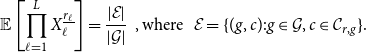 \begin{align*} \mathbb {E}\left [\prod _{\ell =1}^{L}X_\ell ^{\underline {r_\ell }}\right ]=\frac {|\mathcal{E}|}{|\mathcal{G}|}\, \,\textrm {, where }\,\, \mathcal{E}=\{(g,c):g\in \mathcal{G},c\in \mathcal C_{r,g}\}. \end{align*}
Since we have $\ell _s$
distinct variables and constraints in each cycle
$\ell _s$
distinct variables and constraints in each cycle $c_s$
respectively, we can have at most
$c_s$
respectively, we can have at most $\mathfrak l=\sum _{s\in [\mathfrak r]}\ell _s$
distinct variables and constraints in
$\mathfrak l=\sum _{s\in [\mathfrak r]}\ell _s$
distinct variables and constraints in $c$
. Specifically, we only have
$c$
. Specifically, we only have $|V(c)|=\mathfrak l$
variables and
$|V(c)|=\mathfrak l$
variables and $|F(c)|=\mathfrak l$
constraints iff all cycles
$|F(c)|=\mathfrak l$
constraints iff all cycles $c_s$
are disjoint. So, let
$c_s$
are disjoint. So, let
 \begin{align*} \mathcal{E}_0=\{(g,c)\in \mathcal{E}:|V(c)|=|F(c)|=\mathfrak l\} \end{align*}
denote the set of pairs $(g,c)\in \mathcal{E}$
with disjoint cycles and further
$(g,c)\in \mathcal{E}$
with disjoint cycles and further $\mathcal{E}_1=\mathcal{E}\setminus \mathcal{E}_0$
the remaining pairs. Then we have
$\mathcal{E}_1=\mathcal{E}\setminus \mathcal{E}_0$
the remaining pairs. Then we have
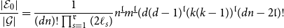 \begin{align*} \frac {|\mathcal{E}_0|}{|\mathcal{G}|} =\frac {1}{(dn)!\prod _{s=1}^{\mathfrak r}(2\ell _s)}n^{\underline {\mathfrak l}}m^{\underline {\mathfrak l}}(d(d-1)^{\mathfrak l}(k(k-1))^{\mathfrak l}(dn-2\mathfrak l)! \end{align*}
for the following reasons. For each cycle $c_s$
in
$c_s$
in $c$
counting the
$c$
counting the $2\ell _s$
directed cycles facilitates the computation, hence we find the corresponding product in the denominator. Since the variables within each directed cycle and the cycles in the sequence are ordered we have an ordered choice of all variables. Further, since the
$2\ell _s$
directed cycles facilitates the computation, hence we find the corresponding product in the denominator. Since the variables within each directed cycle and the cycles in the sequence are ordered we have an ordered choice of all variables. Further, since the $\ell _s$
variables within each cycle are distinct and the cycles are pairwise disjoint we choose all variables without repetition. This explains the first falling factorial. The next term for the constraints follows analogously. But since variables and constraints are disjoint the edges are too, hence we choose two edges for each of the
$\ell _s$
variables within each cycle are distinct and the cycles are pairwise disjoint we choose all variables without repetition. This explains the first falling factorial. The next term for the constraints follows analogously. But since variables and constraints are disjoint the edges are too, hence we choose two edges for each of the $\mathfrak l$
variables and constraints respectively. Then we wire the remaining edges.
$\mathfrak l$
variables and constraints respectively. Then we wire the remaining edges.
The asymptotics are derived analogously to the base case, i.e.
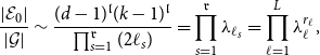 \begin{align*} \frac {|\mathcal{E}_0|}{|\mathcal{G}|} \sim \frac {(d-1)^{\mathfrak l}(k-1)^{\mathfrak l}}{\prod _{s=1}^{\mathfrak r}(2\ell _s)} =\prod _{s=1}^{\mathfrak r}\lambda _{\ell _s}=\prod _{\ell =1}^{L}\lambda _\ell ^{r_\ell }\textrm {,} \end{align*}
using the definition of $c=(c_s)_{s\in [\mathfrak r]}$
in the last step. Since the contribution of the disjoint cycles already yields the desired result, we want to show that the contribution of intersecting cycles is negligible. As before, we count directed cycles
$c=(c_s)_{s\in [\mathfrak r]}$
in the last step. Since the contribution of the disjoint cycles already yields the desired result, we want to show that the contribution of intersecting cycles is negligible. As before, we count directed cycles $\gamma _s$
and adjust the result accordingly, so let
$\gamma _s$
and adjust the result accordingly, so let
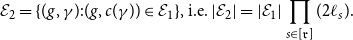 \begin{align*} \mathcal{E}_2=\{(g,\gamma ):(g,c(\gamma ))\in \mathcal{E}_1\}\textrm {, i.e. }|\mathcal{E}_2|=|\mathcal{E}_1|\prod _{s\in [\mathfrak r]}(2\ell _s)\textrm {.} \end{align*}
In the next step we consider the relative position representations $(\alpha, \rho )$
of sequences
$(\alpha, \rho )$
of sequences $\gamma$
of directed cycles. Instead of a formal introduction we illustrate this concept in Figure 3. The corresponding decomposition of the contributions to the expectation according to
$\gamma$
of directed cycles. Instead of a formal introduction we illustrate this concept in Figure 3. The corresponding decomposition of the contributions to the expectation according to $\rho$
is
$\rho$
is
 \begin{align*} \frac {|\mathcal{E}_1|}{|\mathcal{G}|} &=\sum _{\rho \in \mathcal R} \frac {|\mathcal{E}_{\rho }|}{|\mathcal{G}|\prod _{s\in [\mathfrak r]}(2\ell _s)}\textrm {, } \mathcal{E}_{\rho }=\{(g,\gamma )\in \mathcal{E}_2:\rho (\gamma )=\rho \}\textrm {, } \mathcal R=\{\rho (\gamma ):(g,\gamma )\in \mathcal{E}_2\}\textrm {.} \end{align*}
For the following reasons we can then derive
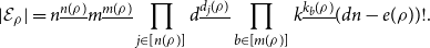 \begin{align*} |\mathcal{E}_{\rho }| =n^{\underline {n(\rho )}}m^{\underline {m(\rho )}} \prod _{j\in [n(\rho )]}d^{\underline {d_j(\rho )}}\prod _{b\in [m(\rho )]}k^{\underline {k_b(\rho )}}(dn-e(\rho ))!\textrm {.} \end{align*}
Since $\rho$
is fixed, we have to fix the absolute values
$\rho$
is fixed, we have to fix the absolute values $\alpha$
, thereby the directed cycle
$\alpha$
, thereby the directed cycle $\gamma$
, and wire the remaining edges. But the first four terms exactly correspond to the number of choices for the index vectors in
$\gamma$
, and wire the remaining edges. But the first four terms exactly correspond to the number of choices for the index vectors in $\alpha$
. This fixes
$\alpha$
. This fixes $\gamma$
, further the union
$\gamma$
, further the union $c(\gamma )$
of cycles and in particular
$c(\gamma )$
of cycles and in particular $e(\rho )$
edges. The remaining term counts the number of choices to wire the remaining edges.
$e(\rho )$
edges. The remaining term counts the number of choices to wire the remaining edges.
For the asymptotics we notice that $n(\rho )$
,
$n(\rho )$
, $m(\rho )\le \mathfrak l$
and that also the two products are bounded in both the multiplication region and values. But this further implies that
$m(\rho )\le \mathfrak l$
and that also the two products are bounded in both the multiplication region and values. But this further implies that $|\mathcal R|$
is bounded, i.e. the summation region is also finite in the limit and hence we can consider the asymptotics of each term separately, which yields
$|\mathcal R|$
is bounded, i.e. the summation region is also finite in the limit and hence we can consider the asymptotics of each term separately, which yields
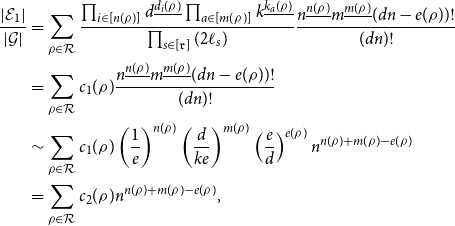 \begin{align*} \frac {|\mathcal{E}_1|}{|\mathcal{G}|} &=\sum _{\rho \in \mathcal R} \frac {\prod _{i\in [n(\rho )]}d^{\underline {d_i(\rho )}}\prod _{a\in [m(\rho )]}k^{\underline {k_a(\rho )}}}{\prod _{s\in [\mathfrak r]}(2\ell _s)} \frac {n^{\underline {n(\rho )}}m^{\underline {m(\rho )}}(dn-e(\rho ))!}{(dn)!}\\ &=\sum _{\rho \in \mathcal R}c_1(\rho ) \frac {n^{\underline {n(\rho )}}m^{\underline {m(\rho )}}(dn-e(\rho ))!}{(dn)!}\\ &\sim \sum _{\rho \in \mathcal R}c_1(\rho ) \left (\frac {1}{e}\right )^{n(\rho )} \left (\frac {d}{ke}\right )^{m(\rho )} \left (\frac {e}{d}\right )^{e(\rho )} n^{n(\rho )+m(\rho )-e(\rho )}\\ &=\sum _{\rho \in \mathcal R}c_2(\rho ) n^{n(\rho )+m(\rho )-e(\rho )}, \end{align*}
where we summarized the terms that only depend on $\rho$
into constants. Now, let
$\rho$
into constants. Now, let $\rho \in \mathcal R$
and let
$\rho \in \mathcal R$
and let $c=c(\rho )$
be the graph of
$c=c(\rho )$
be the graph of $\rho$
as introduced in Section 2.4. Since
$\rho$
as introduced in Section 2.4. Since $\rho$
is a sequence of directed cycles that are not all disjoint, its graph
$\rho$
is a sequence of directed cycles that are not all disjoint, its graph $c$
is the union of the corresponding (undirected) cycles that are not all disjoint. But then
$c$
is the union of the corresponding (undirected) cycles that are not all disjoint. But then $c$
has more edges than vertices, i.e.
$c$
has more edges than vertices, i.e. $3e(\rho )\gt n(\rho )+m(\rho )+2e(\rho )$
, and hence
$3e(\rho )\gt n(\rho )+m(\rho )+2e(\rho )$
, and hence
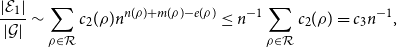 \begin{align*} \frac {|\mathcal{E}_1|}{|\mathcal{G}|} &\sim \sum _{\rho \in \mathcal R}c_2(\rho ) n^{n(\rho )+m(\rho )-e(\rho )} \le n^{-1}\sum _{\rho \in \mathcal R}c_2(\rho ) =c_3n^{-1}\textrm {,} \end{align*}
which shows that this contribution is negligible. This establishes the asymptotic equivalence
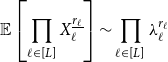 \begin{align*} \mathbb {E}\left [\prod _{\ell \in [L]}X_\ell ^{\underline {r_\ell }}\right ]\sim \prod _{\ell \in [L]}\lambda _\ell ^{r_\ell } \end{align*}
and allows to apply the method of moments, which directly yields Lemma 2.8.


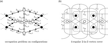


 Open access