


Impact Statement
We present a generic method to optimize trajectories (in a broad sense) under constraints which leverages trajectory data stemming from many data-intensive industries. Through statistical modeling, we include information inferred from data, such as degrees of freedom, constraints, or even correlations between some covariates, into the optimization problem of interest. This restricts in a data-driven way the search space, hence drastically reducing the computational complexity and avoiding to resort to manual editing for dynamics or constraints. While generic, we show it to be of direct interest to two specific settings, namely aeronautics and sailing. The generic nature of the approach motivates further studies to many different data-centric engineering frameworks and industries.
1. Introduction
Optimizing trajectories under constraints appears in many real-world problems. The present paper stems from an initial work on aeronautics and the quest for designing fuel efficient aircraft trajectories based on available flight data. We have reached a generic data-driven methodology which falls in the much broader field of trajectory optimization under constraints. As such, it has potential applications to many more real world problems, such as in robotics to minimize the work-based specific mechanical cost of transport (Srinivasan and Ruina, Reference Srinivasan and Ruina2006) or in aerospace to reduce the total thermal flux when a space shuttle re-enters in the atmosphere (Trélat, Reference Trélat2012).
In aeronautics, optimization problems such as the minimization of the total travel time or the fuel reduction are often formulated in terms of optimal control problems (Codina and Menéndez, Reference Codina and Menéndez2014; Girardet et al., Reference Girardet, Lapasset, Delahaye and Rabut2014; Cots et al., Reference Cots, Gergaud and Goubinat2018). This allows to take into account the dynamics of the system, leading to realistic solutions complying with additional constraints; we refer to Rao (Reference Rao2009) for an overview.
Nevertheless the differential equations describing the dynamics of the system of interest may be (partially) unknown. For instance, the differential system describing the motion of an aircraft moving in an air mass (Rommel et al., Reference Rommel, Bonnans, Martinon and Gregorutti2019) involves the lift and drag forces for which no analytic formulas exist. Aircraft manufacturers typically compute numerical models (not publicly released) by means of heavy simulations and wind tunnel tests. Another approach consists in reconstructing unknown forces based on physical formulas and available flight data; see for instance Rommel et al. (Reference Rommel, Bonnans, Martinon and Gregorutti2017) and Dewez et al. (Reference Dewez, Guedj and Vandewalle2020) for results in aeronautics and Ramsay et al. (Reference Ramsay, Hooker, Campbell and Cao2007) in the generic setting of parameter estimation for differential equations. While promising on paper, this reconstruction step requires restrictive assumptions and the statistical errors may impact strongly the solution of the optimal control problem. Moreover it does not tackle directly the optimization problem.
At the same time, additional safety and air control constraints should be taken into account and modelled so that the optimized trajectory is acceptable for both pilots and air controllers. However such constraints may be numerous and complex to model; we refer to Codina and Menéndez (Reference Codina and Menéndez2014) and Lim et al. (Reference Lim, Gardi, Sabatini, Ranasinghe, Ezer, Rodgers and Salluce2019) for examples of such constraints. Due to the short time for the flight preparation on ground, the execution time to solve numerically such constrained optimization problems may be unacceptable, in particular in the case of nonlinear constraints.
In our work, we propose another kind of approach to provide efficiently realistic trajectories without involving noisy dynamical systems and numerous complex constraints. This is achieved by leveraging available trajectory data. Our approach lies mainly on the estimation of the trajectory distribution, which is assumed to contain intrinsically many information on realistic trajectories. This is then incorporated in the optimization problem of interest through a Bayesian approach, constraining then the problem by the data in a simple and natural way. The main benefit on this approach is that it directly uses the information contained in the data, requiring no explicit information on the dynamics or on additional constraints. This methodology is specific to the situation where the user has access to trajectory data but, at the same time, the approach is intended to be generic enough so that it can be exploited in a wide range of applications. In particular it is certainly not restricted to the aeronautic setting.
The idea of using data to improve optimization processes has been for instance validated by the paper Hewitt and Frejinger (Reference Hewitt and Frejinger2020) in the context of decision support systems. In this paper, the authors are interested in learning mathematical representations of business rules for mixed integer linear programs. Their work is motivated by the development of automatic processes for the implementations of rules given past decision data. Their numerical test cases have shown that such an approach can lead to high-quality decisions with respect to their objective function value while being able to model effectively rules contained in the data. We mention that, apart from the nature of the optimization problems and their applications, the main difference between the methodology in Hewitt and Frejinger (Reference Hewitt and Frejinger2020) and ours is the way we exploit the data: they learn a map sending theoretical optimized decisions to the associated past ones while we incorporate directly estimated features from the data into the optimization problem. In particular, a comparison between these two approaches falls out the scope of this paper. Let us also mention that another strategy could be to leverage purely data-driven reinforcement learning to provide a trajectory (see e.g., Berkenkamp et al., Reference Berkenkamp, Turchetta, Schoellig and Krause2017; Mowbray et al., Reference Mowbray, Petsagkourakis, del Río Chanona and Zhang2021), however, at a considerably higher computational cost.
Let us now give some details on our methodology from a technical point of view. We first assume that all the trajectories belong to a finite-dimensional space, which allows to reduce the complexity of the problem with low information loss for a well-chosen basis. In a Bayesian framework, we assume secondly that the prior distribution of trajectories (through their related coefficients) is proportional to a decreasing exponential function of the cost, assuming that efficient trajectories are a priori more likely than inefficient ones. In our pipeline, the cost function can be especially learnt from the data if necessary. Thirdly we estimate the likelihood distribution which is expected to contain information on realistic trajectories. Here, the observed trajectories, that we call reference trajectories, are interpreted as noisy observations of an efficient one, the noise following a centered Gaussian multivariate distribution. In a Bayesian perspective, it is thus possible to deduce the posterior distribution of the efficient trajectory given the reference trajectories and we focus finally on the mode of this posterior for the sake of simplicity. Under our assumptions, the new objective function involves here the sum between the cost of a trajectory and its squared Mahalanobis distance to a weighted average of reference trajectories. In particular, the resulting optimization problem can be interpreted as a penalized one together with some affine constraints, modeling for instance initial and final conditions.
The role of the likelihood distribution, leading to the penalized term, is to force the solution to be close to real trajectories and so to be likely to comply with the constraints. The strength of the penalization is here controlled by a hyper-parameter and a tuning process is proposed to find an optimal balance between optimization and closeness to the trajectory distribution. Hence, the optimized trajectory may inherit a realistic behavior, even though the dynamics are not explicitly taken into account in our problem.
We mention that the present Gaussian assumption for the likelihood distribution has two advantages. First, it reduces the information on trajectories to the mean trajectory and the covariance matrix, making the results interpretable for experts. In particular, this matrix not only indicates the most unconstrained directions for the optimization, but also reveals linear relations between variables, some of them reflecting the dynamics or being unknown by the user. Second, the Gaussian assumption leads to a penalized term which is actually quadratic. So in certain cases, the problem is convex with affine constraints, allowing to make use of very efficient optimization algorithms.
In a nutshell, this data-driven approach restricts the search space to a region centered on the data in a metric space reflecting features estimated from the data. Further, it is flexible enough to cover not only Gaussian distributions, but also other families of distributions for other kinds of applications. Finally, it is noteworthy that, despite the above hyper-parameter tuning process, the optimized trajectory resulting from our approach may not comply with all the complex constraints of a given real problem, making it unacceptable in practice. To circumvent this issue, one could use for instance our not perfect trajectory as an initial guess in iterative (nonlinear) optimization solvers, which could at the end reduce drastically the number of steps while providing a trajectory fulfilling all the requirements.
1.1. Outline
We describe our approach in Section 2, and briefly discuss its Python implementation (the library PyRotor) in Section 3. Sections 4 and 5 are devoted to applications: the first one to the fuel reduction of aircraft during the climb and the second one to the maximization of the work of a force field along a path. We finish the paper by discussing on future works to improve and generalize our optimization methodology.
2. An End-to-End Optimization Workflow Based on Observed Trajectories
We are interested in finding a trajectory $ {y}^{\star } $
which minimizes a certain cost function
$ {y}^{\star } $
which minimizes a certain cost function $ F $
, namely a solution of the following optimization problem:
$ F $
, namely a solution of the following optimization problem:
 $$ {\tilde{y}}^{\star}\in \underset{y\in {\mathcal{A}}_{\mathcal{G}}\left({y}_0,{y}_T\right)}{\arg \hskip0.1em \min\;}F(y). $$
The set $ {\mathcal{A}}_{\mathcal{G}}\left({y}_0,{y}_T\right) $
, which is defined in Section 2.1, models the constraints the trajectory has to comply with, such that the initial and final conditions or the dynamics. Note that a trajectory is typically a multivariate function defined on an interval and its components are given by states and controls (which are not distinguished in this paper for the sake of presentation). In case of numerous constraints, which is often the case when dealing with real-world applications, the resulting optimization problem (1) may be computationally expensive. On the other hand, a partial knowledge of the constraints may lead to a solution which is by far unrealistic. Adding by hand user-defined constraints might circumvent this issue but may be time-consuming.
$ {\mathcal{A}}_{\mathcal{G}}\left({y}_0,{y}_T\right) $
, which is defined in Section 2.1, models the constraints the trajectory has to comply with, such that the initial and final conditions or the dynamics. Note that a trajectory is typically a multivariate function defined on an interval and its components are given by states and controls (which are not distinguished in this paper for the sake of presentation). In case of numerous constraints, which is often the case when dealing with real-world applications, the resulting optimization problem (1) may be computationally expensive. On the other hand, a partial knowledge of the constraints may lead to a solution which is by far unrealistic. Adding by hand user-defined constraints might circumvent this issue but may be time-consuming.
In view of this, we provide in this section our full workflow to obtain a new optimization problem which includes in a natural and simple way constraints coming from the data. This problem is actually designed to provide trajectories which have a realistic behavior.
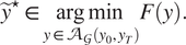
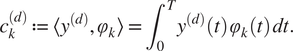
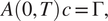
We begin with elementary but necessary definitions for trajectories and constraints in Section 2.1. We aim at stating the optimization problem in a finite basis space so we define in Section 2.2 the mathematical formalization of how we decompose each trajectory as a projection on such a space. To extract information from the data for the optimization problem, a statistical modeling on the projected space of the available trajectory data is done in Section 2. In Section 2.4, we put everything together to obtain our new optimization problem Section 2.4 via a maximum a posteriori (MAP) approach. Section 2.5 presents a handy computation regarding the cost function in a quadratic case, for the sake of completeness. Additional details can be found in the Appendix A. Section 2.6 focuses on a hyper-parameter tuning for an optimal tradeoff between optimization and additional (nonlinear) constraints. Last but not least, Section 2.7 contains confidence intervals to assess the accuracy of the predicted optimized cost when the cost function is known up to a random noise term. We summarize our methodology in Figure 1. We also present an illustrative representation of our pipeline in Figure 2.
Diagram of the global pipeline of our method (solid lines). Dashed lines denote optional components.
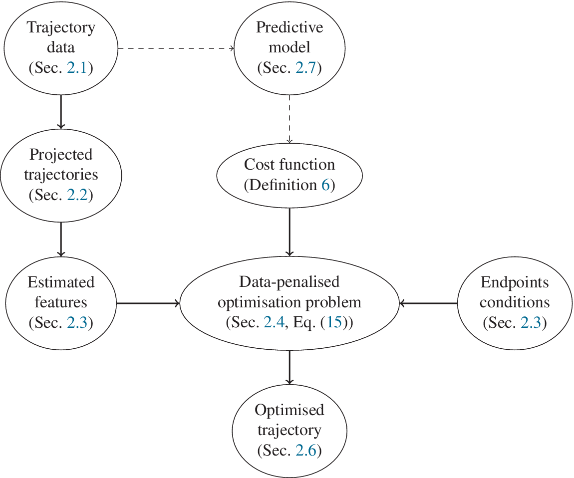
Illustration of our approach. Blue points refer to reference trajectories, the green ellipse is the set of trajectories which is explored to find an optimized trajectory, the red portion is the set of nonadmissible trajectories (e.g., which do not comply with the set of constraints). Note that the size of the green ellipse is automatically adjusted in the process (as discussed in Section 2.6). Dotted lines are the level sets of the cost function (whose minimum is attained in (0,0)) and the optimized trajectory obtained from our method is given by the green point on the boundary of the ellipse.
2.1. Admissible trajectories modeling
We start with definitions.
Definition 1 (Trajectory). Let $ T>0 $
be a real number and let
$ T>0 $
be a real number and let $ D\geqslant 1 $
be an integer. Any continuous
$ D\geqslant 1 $
be an integer. Any continuous $ {\unicode{x211D}}^D $
-valued map
$ {\unicode{x211D}}^D $
-valued map $ y $
defined on
$ y $
defined on $ \left[0,T\right] $
, that is
$ \left[0,T\right] $
, that is $ y\in \mathcal{C}\left(\left[0,T\right],{\unicode{x211D}}^D\right) $
,
Footnote 1
is called a trajectory over the time interval
$ y\in \mathcal{C}\left(\left[0,T\right],{\unicode{x211D}}^D\right) $
,
Footnote 1
is called a trajectory over the time interval $ \left[0,T\right] $
. The
$ \left[0,T\right] $
. The $ d $
th component of a trajectory
$ d $
th component of a trajectory $ y $
will be denoted by
$ y $
will be denoted by $ {y}^{(d)} $
. As such, a trajectory is at least a continuous map on a finite interval.
$ {y}^{(d)} $
. As such, a trajectory is at least a continuous map on a finite interval.
When optimizing a trajectory with respect to a given criterion, the initial and final states are often constrained, that is to say the optimization is performed in an affine subspace modeling these endpoints conditions. This subspace is now introduced.
Definition 2 (Endpoints conditions). Let $ {y}_0,{y}_T\in {\unicode{x211D}}^D $
. We define the set
$ {y}_0,{y}_T\in {\unicode{x211D}}^D $
. We define the set $ \mathcal{D}\left({y}_0,{y}_T\right)\subset \mathcal{C}\left(\left[0,T\right],{\unicode{x211D}}^D\right) $
as
$ \mathcal{D}\left({y}_0,{y}_T\right)\subset \mathcal{C}\left(\left[0,T\right],{\unicode{x211D}}^D\right) $
as
 $$ y\in \mathcal{D}\left({y}_0,{y}_T\right)\hskip2em \iff \hskip2em \left\{\begin{array}{l}y(0)={y}_0,\\ {}y(T)={y}_T.\end{array}\right. $$
In many applications, the trajectories have to satisfy some additional constraints defined by a set of (nonlinear) functions. For instance these functions may model physical or user-defined constraints. We define now the set of trajectories verifying such additional constraints.
Definition 3
(Additional constraints). For $ \mathrm{\ell}=1,\dots, L $
, let
$ \mathrm{\ell}=1,\dots, L $
, let $ {g}_{\mathrm{\ell}} $
be a real-valued function defined on
$ {g}_{\mathrm{\ell}} $
be a real-valued function defined on $ {\unicode{x211D}}^D $
. We define the set
$ {\unicode{x211D}}^D $
. We define the set $ \mathcal{G}\subset \mathcal{C}\left(\left[0,T\right],{\unicode{x211D}}^D\right) $
as the set of trajectories over
$ \mathcal{G}\subset \mathcal{C}\left(\left[0,T\right],{\unicode{x211D}}^D\right) $
as the set of trajectories over $ \left[0,T\right] $
satisfying the following
$ \left[0,T\right] $
satisfying the following $ L $
inequality constraints given by the functions
$ L $
inequality constraints given by the functions $ {g}_{\mathrm{\ell}} $
, that is
$ {g}_{\mathrm{\ell}} $
, that is
 $$ y\in \mathcal{G}\hskip2em \iff \hskip2em \forall \mathrm{\ell}=1,\dots, L\hskip1em \forall t\in \left[0,T\right]\hskip2em {g}_{\mathrm{\ell}}\left(y(t)\right)\leqslant 0. $$
Lastly, we introduce the set of admissible trajectories which satisfy both the endpoints conditions and the additional constraints.
Definition 4 (Admissible trajectory). We define the set $ {\mathcal{A}}_{\mathcal{G}}\left({y}_0,{y}_T\right)\subset \mathcal{C}\left(\left[0,T\right],{\unicode{x211D}}^D\right) $
as follows:
$ {\mathcal{A}}_{\mathcal{G}}\left({y}_0,{y}_T\right)\subset \mathcal{C}\left(\left[0,T\right],{\unicode{x211D}}^D\right) $
as follows:
 $$ {\mathcal{A}}_{\mathcal{G}}\left({y}_0,{y}_T\right):= \mathcal{D}\left({y}_0,{y}_T\right)\cap \mathcal{G}. $$
Any element of $ {\mathcal{A}}_{\mathcal{G}}\left({y}_0,{y}_T\right) $
will be called an admissible trajectory.
$ {\mathcal{A}}_{\mathcal{G}}\left({y}_0,{y}_T\right) $
will be called an admissible trajectory.
2.2. Projection for a finite-dimensional optimization problem
In our approach, a theoretical optimization problem in a finite-dimensional space is desired to reduce the inherent complexity of the problem. This can be achieved by decomposing the trajectories on a finite number of basis functions. While raw signals are unlikely to be described by a small number of parameters, this is not the case for smoothed versions of these signals which capture the important patterns. In particular, given a family of smoothed observed trajectories, one may suppose that there exists a basis such that the projection error on a certain number of basis functions of any trajectory is negligible (i.e., the set of projected trajectories in Figure 1).
From now on, the trajectories we consider are assumed to belong to a space spanned by a finite number of basis functions. For the sake of simplicity, we assume in addition that all the components of the trajectories can be decomposed on the same basis but with different dimensions. Extension to different bases is straightforward and does not change our findings but burdens the notation.
Definition 5.
Let $ {\left\{{\varphi}_k\right\}}_{k=1}^{+\infty } $
be an orthonormal basis of
$ {\left\{{\varphi}_k\right\}}_{k=1}^{+\infty } $
be an orthonormal basis of $ {L}^2\left(\left[0,T\right],\unicode{x211D}\right) $
Footnote 2
with respect to the inner product
$ {L}^2\left(\left[0,T\right],\unicode{x211D}\right) $
Footnote 2
with respect to the inner product
 $$ \left\langle f,g\right\rangle ={\int}_0^Tf(t)\hskip0.1em g(t)\hskip0.1em dt, $$
such that each $ {\varphi}_k $
is continuous on
$ {\varphi}_k $
is continuous on $ \left[0,T\right] $
and let
$ \left[0,T\right] $
and let $ \mathcal{K}:= {\left\{{K}_d\right\}}_{d=1}^D $
be a sequence of integers with
$ \mathcal{K}:= {\left\{{K}_d\right\}}_{d=1}^D $
be a sequence of integers with $ K:= {\sum}_{d=1}^D{K}_d $
. We define the space of projected trajectories
$ K:= {\sum}_{d=1}^D{K}_d $
. We define the space of projected trajectories $ {\mathcal{Y}}_{\mathcal{K}}\left(0,T\right)\subset \mathcal{C}\left(\left[0,T\right],{\unicode{x211D}}^D\right) $
over
$ {\mathcal{Y}}_{\mathcal{K}}\left(0,T\right)\subset \mathcal{C}\left(\left[0,T\right],{\unicode{x211D}}^D\right) $
over $ \left[0,T\right] $
as
$ \left[0,T\right] $
as
 $$ {\mathcal{Y}}_{\mathcal{K}}\left(0,T\right):= \prod \limits_{d=1}^D span{\left\{{\varphi}_k\right\}}_{k=1}^{K_d}. $$
If there is no risk of confusion, we write $ {\mathcal{Y}}_{\mathcal{K}}:= {\mathcal{Y}}_{\mathcal{K}}\left(0,T\right) $
for the sake of readability.
$ {\mathcal{Y}}_{\mathcal{K}}:= {\mathcal{Y}}_{\mathcal{K}}\left(0,T\right) $
for the sake of readability.
Remark 1.
From the above definition, any projected trajectory $ y\in {\mathcal{Y}}_{\mathcal{K}} $
is associated with a unique vector
$ y\in {\mathcal{Y}}_{\mathcal{K}} $
is associated with a unique vector
 $$ c={\left({c}_1^{(1)},\dots, {c}_{K_1}^{(1)},{c}_1^{(2)},\dots, {c}_{K_2}^{(2)},\dots, {c}_1^{(D)},\dots, {c}_{K_D}^{(D)}\right)}^T\in {\unicode{x211D}}^K $$
defined by
 $$ {c}_k^{(d)}:= \left\langle {y}^{(d)},{\varphi}_k\right\rangle ={\int}_0^T{y}^{(d)}(t)\hskip0.1em {\varphi}_k(t)\hskip0.1em dt. $$
In other words, the vector $ c $
is the image of the trajectory
$ c $
is the image of the trajectory $ y $
by the projection operator
$ y $
by the projection operator $ \Phi :\mathcal{C}\left(\left[0,T\right],{\unicode{x211D}}^D\right)\to {\unicode{x211D}}^K $
defined by
$ \Phi :\mathcal{C}\left(\left[0,T\right],{\unicode{x211D}}^D\right)\to {\unicode{x211D}}^K $
defined by $ \Phi y:= c $
, whose restriction
$ \Phi y:= c $
, whose restriction $ {\left.\Phi \right|}_{{\mathcal{Y}}_{\mathcal{K}}} $
is bijective (as the Cartesian product of bijective operators). In particular, the spaces
$ {\left.\Phi \right|}_{{\mathcal{Y}}_{\mathcal{K}}} $
is bijective (as the Cartesian product of bijective operators). In particular, the spaces $ {\mathcal{Y}}_{\mathcal{K}} $
and
$ {\mathcal{Y}}_{\mathcal{K}} $
and $ {\unicode{x211D}}^K $
are isomorphic, that is
$ {\unicode{x211D}}^K $
are isomorphic, that is $ {\mathcal{Y}}_{\mathcal{K}}\simeq {\unicode{x211D}}^K $
.
$ {\mathcal{Y}}_{\mathcal{K}}\simeq {\unicode{x211D}}^K $
.
Regarding the endpoints conditions introduced in Definition 2, we prove in the following result that satisfying these conditions is equivalent to satisfying a linear system for a projected trajectory.
Proposition 1.
A trajectory $ y\in {\mathcal{Y}}_{\mathcal{K}} $
belongs to
$ y\in {\mathcal{Y}}_{\mathcal{K}} $
belongs to $ \mathcal{D}\left({y}_0,{y}_T\right) $
if and only if its associated vector
$ \mathcal{D}\left({y}_0,{y}_T\right) $
if and only if its associated vector $ c:= \Phi y\in {\unicode{x211D}}^K $
satisfies the linear system
$ c:= \Phi y\in {\unicode{x211D}}^K $
satisfies the linear system
 $$ A\left(0,T\right)\hskip0.1em c=\Gamma, $$
where the matrix $ A\left(0,T\right)\in {\unicode{x211D}}^{2D\times K} $
and the vector
$ A\left(0,T\right)\in {\unicode{x211D}}^{2D\times K} $
and the vector $ \Gamma \in {\unicode{x211D}}^{2D} $
are given by
$ \Gamma \in {\unicode{x211D}}^{2D} $
are given by
 $$ A\left(0,T\right):= \left(\begin{array}{ccccccc}{\varphi}_1(0)& \dots & {\varphi}_{K_1}(0)& & & & \\ {}& & & \ddots & & & \\ {}& & & & {\varphi}_1(0)& \dots & {\varphi}_{K_D}(0)\\ {}{\varphi}_1(T)& \dots & {\varphi}_{K_1}(T)& & & & \\ {}& & & \ddots & & & \\ {}& & & & {\varphi}_1(T)& \dots & {\varphi}_{K_D}(T)\end{array}\right)\hskip1em ,\hskip1em \Gamma := \left(\begin{array}{c}{y}_0\\ {}{y}_T\end{array}\right). $$
Proof. Let $ y\in {\mathcal{Y}}_{\mathcal{K}} $
and let
$ y\in {\mathcal{Y}}_{\mathcal{K}} $
and let $ c:= \Phi y\in {\unicode{x211D}}^K $
. By the definition of the matrix
$ c:= \Phi y\in {\unicode{x211D}}^K $
. By the definition of the matrix $ A\left(0,T\right) $
, we have
$ A\left(0,T\right) $
, we have
 $$ {\displaystyle \begin{array}{c}A\left(0,T\right)\hskip0.1em c=A\left(0,T\right){\left({c}_1^{(1)},\dots, {c}_{K_1}^{(1)},{c}_1^{(2)},\dots, {c}_{K_2}^{(2)},\dots, {c}_1^{(D)},\dots, {c}_{K_D}^{(D)}\right)}^T\\ {}\hskip18.9em ={\left(\sum \limits_{k=1}^{K_1}{c}_k^{(1)}{\varphi}_k(0),\dots, \sum \limits_{k=1}^{K_D}{c}_k^{(D)}{\varphi}_k(0),\dots, \sum \limits_{k=1}^{K_1}{c}_k^{(1)}{\varphi}_k(T),\dots, \sum \limits_{k=1}^{K_D}{c}_k^{(D)}{\varphi}_k(T)\right)}^T\\ {}\hskip-21.5em =\left(\begin{array}{c}y(0)\\ {}y(T)\end{array}\right).\end{array}} $$
The conclusion follows directly from the preceding relation.
2.3. Reference trajectories modeling
Let us now suppose that we have access to $ I $
recorded trajectories
$ I $
recorded trajectories $ {y}_{R_1},\dots, {y}_{R_I} $
, called reference trajectories, coming from some experiments. We propose here an example of a statistical modeling for these reference trajectories, permitting especially to exhibit some linear properties. This modeling will allow to take advantage of the information contained in these recorded trajectories when deriving optimization problems.
$ {y}_{R_1},\dots, {y}_{R_I} $
, called reference trajectories, coming from some experiments. We propose here an example of a statistical modeling for these reference trajectories, permitting especially to exhibit some linear properties. This modeling will allow to take advantage of the information contained in these recorded trajectories when deriving optimization problems.
These trajectories being recorded, they are in particular admissible and we assume that they belong to the space $ {\mathcal{Y}}_{\mathcal{K}}\left(0,T\right) $
. As explained previously they may be interpreted as smoothed versions of recorded signals. In particular, each reference trajectory
$ {\mathcal{Y}}_{\mathcal{K}}\left(0,T\right) $
. As explained previously they may be interpreted as smoothed versions of recorded signals. In particular, each reference trajectory $ {y}_{R_i} $
is associated with a unique vector
$ {y}_{R_i} $
is associated with a unique vector $ {c}_{R_i}\in {\unicode{x211D}}^K $
. Moreover, we consider each reference trajectory as a noisy observation of a certain admissible and projected trajectory
$ {c}_{R_i}\in {\unicode{x211D}}^K $
. Moreover, we consider each reference trajectory as a noisy observation of a certain admissible and projected trajectory $ {y}_{\ast } $
. In other words, we suppose that there exists a trajectory
$ {y}_{\ast } $
. In other words, we suppose that there exists a trajectory $ {y}_{\ast}\in {\mathcal{Y}}_{\mathcal{K}}\cap {\mathcal{A}}_{\mathcal{G}}\left({y}_0,{y}_T\right) $
associated with a vector
$ {y}_{\ast}\in {\mathcal{Y}}_{\mathcal{K}}\cap {\mathcal{A}}_{\mathcal{G}}\left({y}_0,{y}_T\right) $
associated with a vector $ {c}_{\ast}\in {\unicode{x211D}}^K $
satisfying
$ {c}_{\ast}\in {\unicode{x211D}}^K $
satisfying
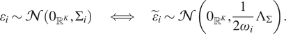
 $$ \forall i=1,\dots, I\hskip2em {c}_{R_i}={c}_{\ast }+{\varepsilon}_i. $$
The noise $ {\varepsilon}_i $
is here assumed to be a centered GaussianFootnote
3 whose covariance matrix
$ {\varepsilon}_i $
is here assumed to be a centered GaussianFootnote
3 whose covariance matrix $ {\Sigma}_i $
is of the form
$ {\Sigma}_i $
is of the form
 $$ {\Sigma}_i=\frac{1}{2{\omega}_i}\hskip0.1em \Sigma, $$
where $ \Sigma \in {\unicode{x211D}}^{K\times K} $
. It is noteworthy that this matrix will not be known in most of the cases but an estimated covariance matrix can be computed on the basis of the reference vectors. The positive real numbers
$ \Sigma \in {\unicode{x211D}}^{K\times K} $
. It is noteworthy that this matrix will not be known in most of the cases but an estimated covariance matrix can be computed on the basis of the reference vectors. The positive real numbers $ {\omega}_i $
are here considered as weights so we require
$ {\omega}_i $
are here considered as weights so we require $ {\sum}_{i=1}^I{\omega}_i=1 $
; each
$ {\sum}_{i=1}^I{\omega}_i=1 $
; each $ {\omega}_i $
plays actually the role of a noise intensity. Further from the hypothesis that the trajectory
$ {\omega}_i $
plays actually the role of a noise intensity. Further from the hypothesis that the trajectory $ {y}_{\ast } $
and all the reference trajectories
$ {y}_{\ast } $
and all the reference trajectories $ {y}_{R_i} $
verify the same endpoints conditions, we deduce
$ {y}_{R_i} $
verify the same endpoints conditions, we deduce
 $$ A\hskip0.1em {c}_{R_i}=A\hskip0.1em {c}_{\ast }+A\hskip0.1em {\varepsilon}_i\hskip2em \iff \hskip2em A\hskip0.1em {\varepsilon}_i={0}_{{\unicode{x211D}}^{2D}}\hskip2em \iff \hskip2em {\varepsilon}_i\in \ker A, $$
for all $ i=1,\dots, I $
(we shorten
$ i=1,\dots, I $
(we shorten $ A\left(0,T\right) $
in
$ A\left(0,T\right) $
in $ A $
when the context is clear). Hence, the reference vector
$ A $
when the context is clear). Hence, the reference vector $ {c}_{\ast } $
satisfies the following
$ {c}_{\ast } $
satisfies the following $ I $
systems:
$ I $
systems:
 $$ \left\{\begin{array}{l}{c}_{R_i}={c}_{\ast }+{\varepsilon}_i,\\ {}{\varepsilon}_i\sim \mathcal{N}\left({0}_{{\unicode{x211D}}^K},{\Sigma}_i\right)\\ {}{\varepsilon}_i\in \ker A.\end{array}\right., $$
To establish a more explicit system which is equivalent to the preceding one, we require the following preliminary proposition. Here, we diagonalize the matrices $ \Sigma $
and
$ \Sigma $
and $ {A}^TA $
by exploiting the fact that the image of the first one is contained in the null space of the other one and vice versa; this is shown in the proof. This property is actually a consequence of the above modeling: the endpoints conditions modelled by
$ {A}^TA $
by exploiting the fact that the image of the first one is contained in the null space of the other one and vice versa; this is shown in the proof. This property is actually a consequence of the above modeling: the endpoints conditions modelled by $ A $
imply linear relations within the components of the vectors, which should be reflected by the covariance matrix
$ A $
imply linear relations within the components of the vectors, which should be reflected by the covariance matrix $ \Sigma $
. The following result will be helpful to establish the upcoming proposition 3.
$ \Sigma $
. The following result will be helpful to establish the upcoming proposition 3.
Proposition 2.
We define $ \sigma := \mathit{\operatorname{rank}}\hskip0.1em \Sigma $
and
$ \sigma := \mathit{\operatorname{rank}}\hskip0.1em \Sigma $
and $ a:= \mathit{\operatorname{rank}}\hskip0.1em {A}^TA $
. In the setting of system (4), we have
$ a:= \mathit{\operatorname{rank}}\hskip0.1em {A}^TA $
. In the setting of system (4), we have $ \sigma +a\leqslant K $
and there exist an orthogonal matrix
$ \sigma +a\leqslant K $
and there exist an orthogonal matrix $ V\in {\unicode{x211D}}^{K\times K} $
and two matrices
$ V\in {\unicode{x211D}}^{K\times K} $
and two matrices $ {\Lambda}_{\Sigma}\in {\unicode{x211D}}^{K\times K} $
and
$ {\Lambda}_{\Sigma}\in {\unicode{x211D}}^{K\times K} $
and $ {\Lambda}_A\in {\unicode{x211D}}^{K\times K} $
of the following form:
$ {\Lambda}_A\in {\unicode{x211D}}^{K\times K} $
of the following form:
 $$ {\Lambda}_{\Sigma}=\left(\begin{array}{cc}{\Lambda}_{\Sigma, 1}& {0}_{{\unicode{x211D}}^{\sigma \times \left(K-\sigma \right)}}\\ {}{0}_{{\unicode{x211D}}^{\left(K-\sigma \right)\times \sigma }}& {0}_{{\unicode{x211D}}^{\left(K-\sigma \right)\times \left(K-\sigma \right)}}\end{array}\right)\hskip2em ,\hskip2em {\Lambda}_A=\left(\begin{array}{cc}{0}_{{\unicode{x211D}}^{\left(K-a\right)\times \left(K-a\right)}}& {0}_{{\unicode{x211D}}^{\left(K-a\right)\times a}}\\ {}{0}_{{\unicode{x211D}}^{a\times \left(K-a\right)}}& {\Lambda}_{A,2}\end{array}\right), $$
where $ {\Lambda}_{\Sigma, 1}\in {\unicode{x211D}}^{\sigma \times \sigma } $
and
$ {\Lambda}_{\Sigma, 1}\in {\unicode{x211D}}^{\sigma \times \sigma } $
and $ {\Lambda}_{A,2}\in {\unicode{x211D}}^{a\times a} $
are diagonal matrices with positive elements, such that
$ {\Lambda}_{A,2}\in {\unicode{x211D}}^{a\times a} $
are diagonal matrices with positive elements, such that
 $$ \Sigma =V{\Lambda}_{\Sigma}{V}^T\hskip2em ,\hskip2em {A}^TA=V{\Lambda}_A{V}^T. $$
Proof. The proof starts by noticing
 $$ \Sigma \hskip0.1em {A}^TA={A}^TA\hskip0.1em \Sigma ={0}_{{\unicode{x211D}}^{K\times K}}. $$
Indeed using the hypothesis $ {\varepsilon}_i\in \ker \hskip0.5em A $
for any
$ {\varepsilon}_i\in \ker \hskip0.5em A $
for any $ i=1,\dots, I $
gives
$ i=1,\dots, I $
gives
 $$ \Sigma \hskip0.1em {A}^TA=2{\omega}_i\hskip0.1em {\Sigma}_i\hskip0.1em {A}^TA=2{\omega}_i\hskip0.1em \unicode{x1D53C}\left({\varepsilon}_i{\varepsilon}_i^T\right)\hskip0.1em {A}^TA=2{\omega}_i\hskip0.1em \unicode{x1D53C}\left({\varepsilon}_i\hskip0.1em {\left(A{\varepsilon}_i\right)}^T\right)\hskip0.1em A={0}_{{\unicode{x211D}}^{K\times K}}; $$
similar arguments prove the second equality in (5). First, we can deduce
 $$ \operatorname{Im}\hskip0.3em \Sigma \hskip0.3em \subseteq \hskip0.3em \ker \hskip0.3em {A}^TA, $$
which leads to $ \sigma \leqslant K-a $
by the rank-nullity theorem. Equalities (5) show also that
$ \sigma \leqslant K-a $
by the rank-nullity theorem. Equalities (5) show also that $ \Sigma $
and
$ \Sigma $
and $ {A}^TA $
are simultaneously diagonalizable (since they commute) so there exists an orthogonal matrix
$ {A}^TA $
are simultaneously diagonalizable (since they commute) so there exists an orthogonal matrix $ V\in {\unicode{x211D}}^{K\times K} $
such that
$ V\in {\unicode{x211D}}^{K\times K} $
such that
 $$ \Sigma =V{\Lambda}_{\Sigma}{V}^T\hskip2em ,\hskip2em {A}^TA=V{\Lambda}_A{V}^T, $$
where $ {\Lambda}_{\Sigma}\in {\unicode{x211D}}^{K\times K} $
and
$ {\Lambda}_{\Sigma}\in {\unicode{x211D}}^{K\times K} $
and $ {\Lambda}_A\in {\unicode{x211D}}^{K\times K} $
are diagonal matrices. Permuting if necessary columns of
$ {\Lambda}_A\in {\unicode{x211D}}^{K\times K} $
are diagonal matrices. Permuting if necessary columns of $ V $
, we can write the matrix
$ V $
, we can write the matrix $ {\Lambda}_{\Sigma} $
as follows:
$ {\Lambda}_{\Sigma} $
as follows:
 $$ {\Lambda}_{\Sigma}=\left(\begin{array}{cc}{\Lambda}_{\Sigma, 1}& {0}_{{\unicode{x211D}}^{\sigma \times \left(K-\sigma \right)}}\\ {}{0}_{{\unicode{x211D}}^{\left(K-\sigma \right)\times \sigma }}& {0}_{{\unicode{x211D}}^{\left(K-\sigma \right)\times \left(K-\sigma \right)}}\end{array}\right); $$
in other words, the $ \sigma $
first column vectors of
$ \sigma $
first column vectors of $ V $
span the image of
$ V $
span the image of $ \Sigma $
. From the inclusion (6), we deduce that these vectors belong to the null space of
$ \Sigma $
. From the inclusion (6), we deduce that these vectors belong to the null space of $ {A}^TA $
. Hence, the
$ {A}^TA $
. Hence, the $ \sigma $
first diagonal elements of
$ \sigma $
first diagonal elements of $ {\Lambda}_A $
are equal to zero and, up to a permutation of the
$ {\Lambda}_A $
are equal to zero and, up to a permutation of the $ K-\sigma $
last column vectors of
$ K-\sigma $
last column vectors of $ V $
, we can write
$ V $
, we can write
 $$ {\Lambda}_A=\left(\begin{array}{cc}{0}_{{\unicode{x211D}}^{\left(K-a\right)\times \left(K-a\right)}}& {0}_{{\unicode{x211D}}^{\left(K-a\right)\times a}}\\ {}{0}_{{\unicode{x211D}}^{a\times \left(K-a\right)}}& {\Lambda}_{A,2}\end{array}\right), $$
which ends the proof. □
Remark 2. From equalities (5), we can also deduce
 $$ \operatorname{Im}\hskip0.5em {A}^TA\subseteq \ker \hskip0.3em \Sigma, $$
showing that $ \Sigma $
is singular. Consequently the Gaussian noise
$ \Sigma $
is singular. Consequently the Gaussian noise $ {\varepsilon}_i $
involved in (4) is degenerate.
$ {\varepsilon}_i $
involved in (4) is degenerate.
A new formulation of system (4) which makes explicit the constrained and unconstrained parts of a vector satisfying this system is given in the following result. This is achieved using the preceding result which allows to decompose the space $ {\unicode{x211D}}^K $
into three orthogonal subspaces. We prove that the restriction of the noise
$ {\unicode{x211D}}^K $
into three orthogonal subspaces. We prove that the restriction of the noise $ {\varepsilon}_i $
to the first subspace is a non-degenerate Gaussian, showing that this first subspace corresponds to the unconstrained one. The two other subspaces describe affine relations coming from the endpoints conditions and from implicit relations within the vector components. These implicit relations, which may model for instance natural trends, are expected to be contained in the reference vectors
$ {\varepsilon}_i $
to the first subspace is a non-degenerate Gaussian, showing that this first subspace corresponds to the unconstrained one. The two other subspaces describe affine relations coming from the endpoints conditions and from implicit relations within the vector components. These implicit relations, which may model for instance natural trends, are expected to be contained in the reference vectors $ {c}_{R_i} $
and reflected by the (estimated) covariance matrix
$ {c}_{R_i} $
and reflected by the (estimated) covariance matrix $ \Sigma $
.
$ \Sigma $
.
Prior to this, let us write the matrix $ V\in {\unicode{x211D}}^{K\times K} $
introduced in Proposition 2 as follows:
$ V\in {\unicode{x211D}}^{K\times K} $
introduced in Proposition 2 as follows:
 $$ V=\left({V}_1\hskip1em {V}_2\hskip1em {V}_3\right), $$
where $ {V}_1\in {\unicode{x211D}}^{K\times \sigma } $
,
$ {V}_1\in {\unicode{x211D}}^{K\times \sigma } $
, $ {V}_2\in {\unicode{x211D}}^{K\times K-\sigma -a} $
and
$ {V}_2\in {\unicode{x211D}}^{K\times K-\sigma -a} $
and $ {V}_3\in {\unicode{x211D}}^{K\times a} $
. We emphasize that the column-vectors of the matrices
$ {V}_3\in {\unicode{x211D}}^{K\times a} $
. We emphasize that the column-vectors of the matrices $ {V}_1 $
and
$ {V}_1 $
and $ {V}_3 $
do not overlap according to the property
$ {V}_3 $
do not overlap according to the property $ \sigma +a\leqslant K $
proved in proposition 2. In particular, the matrix
$ \sigma +a\leqslant K $
proved in proposition 2. In particular, the matrix $ {V}_2 $
has to be considered only in the case
$ {V}_2 $
has to be considered only in the case $ \sigma +a<K $
. Further for any
$ \sigma +a<K $
. Further for any $ c\in {\unicode{x211D}}^K $
, we will use the notation
$ c\in {\unicode{x211D}}^K $
, we will use the notation
 $$ \tilde{c}:= {V}^Tc\hskip2em ,\hskip2em {\tilde{c}}_{\mathrm{\ell}}:= {V}_{\mathrm{\ell}}^Tc, $$
for $ \mathrm{\ell}=\mathrm{1,2,3} $
. Finally, we consider the singular value decomposition of
$ \mathrm{\ell}=\mathrm{1,2,3} $
. Finally, we consider the singular value decomposition of $ A $
coming from the diagonalization of the symmetric matrix
$ A $
coming from the diagonalization of the symmetric matrix $ {A}^TA $
with
$ {A}^TA $
with $ V $
:
$ V $
:
 $$ A={US}_A{V}^T, $$
where $ U\in {\unicode{x211D}}^{2D\times 2D} $
is orthogonal and
$ U\in {\unicode{x211D}}^{2D\times 2D} $
is orthogonal and $ {S}_A\in {\unicode{x211D}}^{2D\times K} $
is a rectangular diagonal matrix of the following form:
$ {S}_A\in {\unicode{x211D}}^{2D\times K} $
is a rectangular diagonal matrix of the following form:
 $$ {S}_A=\left({0}_{{\unicode{x211D}}^{2D\times K-2D}}\hskip1em {S}_{A,2}\right), $$
with $ {S}_{A,2}:= \sqrt{\Lambda_{A,2}}\in {\unicode{x211D}}^{2D\times 2D} $
.
$ {S}_{A,2}:= \sqrt{\Lambda_{A,2}}\in {\unicode{x211D}}^{2D\times 2D} $
.
Proposition 3.
Suppose that the matrix $ A $
is full rank, that is
$ A $
is full rank, that is $ a=2D $
. Then for any
$ a=2D $
. Then for any $ i=1,\dots, I $
, system (4) is equivalent to the following one:
$ i=1,\dots, I $
, system (4) is equivalent to the following one:
 $$ \left\{\begin{array}{l}{\tilde{c}}_{R_i,1}={\tilde{c}}_{\ast, 1}+{\tilde{\varepsilon}}_{i,1},\\ {}{\tilde{\varepsilon}}_{i,1}\sim \mathcal{N}\left({0}_{{\unicode{x211D}}^{\sigma }},\frac{1}{2{\omega}_i}\hskip0.1em {\Lambda}_{\Sigma, 1}\right)\\ {}{\tilde{c}}_{\ast, 2}={V}_2^T{c}_{R_i},\\ {}{\tilde{c}}_{\ast, 3}={S}_{A,2}^{-1}\hskip0.1em {U}^T\Gamma .\end{array},\right. $$
Proof. We first prove that system (4) is equivalent to
 $$ \left\{\begin{array}{l}{\tilde{c}}_{R_i}={\tilde{c}}_{\ast }+{\tilde{\varepsilon}}_i,\\ {}{\tilde{\varepsilon}}_i\sim \mathcal{N}\left({0}_{{\unicode{x211D}}^K},\frac{1}{2{\omega}_i}\hskip0.1em {\Lambda}_{\Sigma}\right)\\ {}{S}_A{\tilde{c}}_{\ast }={U}^T\Gamma .\end{array}\right., $$
The matrix $ V $
being orthogonal, it is nonsingular and so we have for all
$ V $
being orthogonal, it is nonsingular and so we have for all $ i=1,\dots, I $
,
$ i=1,\dots, I $
,
 $$ {c}_{R_i}={c}_{\ast }+{\varepsilon}_i\hskip2em \iff \hskip2em {\tilde{c}}_{R_i}={\tilde{c}}_{\ast }+{\tilde{\varepsilon}}_i, $$
and, since $ {\Sigma}_i=\frac{1}{2{\omega}_i}\hskip0.1em \Sigma =\frac{1}{2{\omega}_i}\hskip0.1em V{\Lambda}_{\Sigma}{V}^T $
, we obtain
$ {\Sigma}_i=\frac{1}{2{\omega}_i}\hskip0.1em \Sigma =\frac{1}{2{\omega}_i}\hskip0.1em V{\Lambda}_{\Sigma}{V}^T $
, we obtain
 $$ {\varepsilon}_i\sim \mathcal{N}\left({0}_{{\unicode{x211D}}^K},{\Sigma}_i\right)\hskip2em \iff \hskip2em {\tilde{\varepsilon}}_i\sim \mathcal{N}\left({0}_{{\unicode{x211D}}^K},\frac{1}{2{\omega}_i}\hskip0.1em {\Lambda}_{\Sigma}\right). $$
Finally, the property $ {\varepsilon}_i\in \ker \hskip0.3em A $
is equivalent to
$ {\varepsilon}_i\in \ker \hskip0.3em A $
is equivalent to
 $$ A\hskip0.1em {c}_{\ast }=\Gamma \hskip2em \iff \hskip2em {US}_A{V}^T{c}_{\ast }=\Gamma \hskip2em \iff \hskip2em {S}_A\hskip0.1em {\tilde{c}}_{\ast }={U}^T\Gamma, $$
proving that the systems (4) and (11) are equivalent. Now the fact that the $ K-\sigma $
last diagonal elements of
$ K-\sigma $
last diagonal elements of $ {\Lambda}_{\Sigma} $
are zero implies that the components
$ {\Lambda}_{\Sigma} $
are zero implies that the components $ {\tilde{c}}_{\ast, 2}\in {\unicode{x211D}}^{K-\sigma -2D} $
and
$ {\tilde{c}}_{\ast, 2}\in {\unicode{x211D}}^{K-\sigma -2D} $
and $ {\tilde{c}}_{\ast, 3}\in {\unicode{x211D}}^{2D} $
are constant. From the first equality of (11), we have on one side
$ {\tilde{c}}_{\ast, 3}\in {\unicode{x211D}}^{2D} $
are constant. From the first equality of (11), we have on one side
 $$ {\tilde{c}}_{R_i,2}={\tilde{c}}_{\ast, 2}\hskip2em \iff \hskip2em {V}_2^T{c}_{R_i}={\tilde{c}}_{\ast, 2}, $$
for any $ i=1,\dots, I $
. On the other side, combining the last relation of the system (11) with the form of the matrix
$ i=1,\dots, I $
. On the other side, combining the last relation of the system (11) with the form of the matrix $ {S}_A $
given in (9) yields
$ {S}_A $
given in (9) yields
 $$ {\displaystyle \begin{array}{l}{S}_A\hskip0.1em {\tilde{c}}_{\ast }={U}^T\Gamma \hskip2em \iff \hskip2em {S}_{A,2}\hskip0.1em {\tilde{c}}_{\ast, 3}={U}^T\Gamma \\ {}\hskip10em \iff \hskip2em {\tilde{c}}_{\ast, 3}={S}_{A,2}^{-1}\hskip0.1em {U}^T\Gamma, \end{array}} $$
the last equivalence being justified by the hypothesis that the matrix $ A $
is full rank (which implies that the diagonal matrix
$ A $
is full rank (which implies that the diagonal matrix $ {S}_{A,2} $
is nonsingular).□
$ {S}_{A,2} $
is nonsingular).□
The above decomposition gives us access to nondegenerated density of $ {\tilde{c}}_{R_i,1} $
given
$ {\tilde{c}}_{R_i,1} $
given $ {\tilde{c}}_{\ast, 1} $
which is later denoted by
$ {\tilde{c}}_{\ast, 1} $
which is later denoted by $ u\left({\tilde{c}}_{R_i,1}|{\tilde{c}}_{\ast, 1}\right) $
. In next section, we will assume a prior distribution on
$ u\left({\tilde{c}}_{R_i,1}|{\tilde{c}}_{\ast, 1}\right) $
. In next section, we will assume a prior distribution on $ {\tilde{c}}_{\ast, 1} $
with high density for low values of the cost function
$ {\tilde{c}}_{\ast, 1} $
with high density for low values of the cost function $ F $
.
$ F $
.
2.4. A trajectory optimization problem via a MAP approach
Before introducing the Bayesian framework, let first recall that we are interested in minimizing a certain cost function $ F:\mathcal{C}\left(\left[0,T\right],{\unicode{x211D}}^D\right)\to \unicode{x211D} $
over the set of projected and admissible trajectories
$ F:\mathcal{C}\left(\left[0,T\right],{\unicode{x211D}}^D\right)\to \unicode{x211D} $
over the set of projected and admissible trajectories $ {\mathcal{Y}}_{\mathcal{K}}\cap {\mathcal{A}}_{\mathcal{G}}\left({y}_0,{y}_T\right) $
. As explained previously, we propose here a methodology leading to a constrained optimization problem based on the reference trajectories and designed to provide realistic trajectories (we refer again to Figure 1). Technically speaking, we seek for the mode of a posterior distribution which contains information from the reference trajectories. The aim of this subsection is then to obtain the posterior distribution via Bayes’s rule, using in particular the precise modeling of the reference trajectories given in Proposition 3 and defining an accurate prior distribution with high density for low values of the cost function
$ {\mathcal{Y}}_{\mathcal{K}}\cap {\mathcal{A}}_{\mathcal{G}}\left({y}_0,{y}_T\right) $
. As explained previously, we propose here a methodology leading to a constrained optimization problem based on the reference trajectories and designed to provide realistic trajectories (we refer again to Figure 1). Technically speaking, we seek for the mode of a posterior distribution which contains information from the reference trajectories. The aim of this subsection is then to obtain the posterior distribution via Bayes’s rule, using in particular the precise modeling of the reference trajectories given in Proposition 3 and defining an accurate prior distribution with high density for low values of the cost function $ F $
.
$ F $
.
To do so, we recall firstly that all the trajectories considered here are assumed to belong to the space $ {\mathcal{Y}}_{\mathcal{K}} $
which is isomorphic to
$ {\mathcal{Y}}_{\mathcal{K}} $
which is isomorphic to $ {\unicode{x211D}}^K $
. So each trajectory is here described by its associated vector in
$ {\unicode{x211D}}^K $
. So each trajectory is here described by its associated vector in $ {\unicode{x211D}}^K $
, permitting in particular to define distributions over finite-dimensional spaces. We also recall that the reference trajectories are interpreted as noisy observations of a certain
$ {\unicode{x211D}}^K $
, permitting in particular to define distributions over finite-dimensional spaces. We also recall that the reference trajectories are interpreted as noisy observations of a certain $ {y}_{\ast } $
associated with a
$ {y}_{\ast } $
associated with a $ {c}_{\ast } $
. According to Proposition 3, this vector complies with some affine conditions which are described by the following subspace
$ {c}_{\ast } $
. According to Proposition 3, this vector complies with some affine conditions which are described by the following subspace $ {\mathcal{V}}_1 $
:
$ {\mathcal{V}}_1 $
:
 $$ c\in {\mathcal{V}}_1\hskip2em \iff \hskip2em \left\{\begin{array}{l}{V}_2^Tc={V}_2^T{c}_{R_i},\\ {}{V}_3^Tc={S}_{A,2}^{-1}\hskip0.1em {U}^T\Gamma .\end{array}\right. $$
Hence, a vector $ c $
belonging to
$ c $
belonging to $ {\mathcal{V}}_1 $
is described only through its component
$ {\mathcal{V}}_1 $
is described only through its component $ {\tilde{c}}_1:= {V}_1^Tc $
. In addition, we note that the definition of
$ {\tilde{c}}_1:= {V}_1^Tc $
. In addition, we note that the definition of $ {\mathcal{V}}_1 $
does not depend actually on the choice of
$ {\mathcal{V}}_1 $
does not depend actually on the choice of $ i $
since
$ i $
since $ {V}_2^T{c}_{R_i} $
has been proved to be constant in Proposition 3. Further, we emphasize that the matrix
$ {V}_2^T{c}_{R_i} $
has been proved to be constant in Proposition 3. Further, we emphasize that the matrix $ A $
is supposed to be full rank in this case and we have
$ A $
is supposed to be full rank in this case and we have $ {\mathcal{V}}_1\simeq {\unicode{x211D}}^{\sigma } $
; we recall that
$ {\mathcal{V}}_1\simeq {\unicode{x211D}}^{\sigma } $
; we recall that $ \sigma $
is the rank of the covariance matrix
$ \sigma $
is the rank of the covariance matrix $ \Sigma $
.
$ \Sigma $
.
Let us now define the cost function $ F $
over the spaces
$ F $
over the spaces $ {\unicode{x211D}}^K $
and
$ {\unicode{x211D}}^K $
and $ {\mathcal{V}}_1 $
. This is necessary to define the prior distribution and to establish our optimization problem.
$ {\mathcal{V}}_1 $
. This is necessary to define the prior distribution and to establish our optimization problem.
Definition 6 (Cost functions). Let $ \overset{\check{}}{F}:{\unicode{x211D}}^K\to \unicode{x211D} $
and
$ \overset{\check{}}{F}:{\unicode{x211D}}^K\to \unicode{x211D} $
and $ \tilde{F}:{\unicode{x211D}}^{\sigma}\to \unicode{x211D} $
be
$ \tilde{F}:{\unicode{x211D}}^{\sigma}\to \unicode{x211D} $
be
-
• $ {\left.\overset{\check{}}{F}(c):= F\Big(\Phi \right|}_{{\mathcal{Y}}_{\mathcal{K}}}^{-1}c\Big) $
;
$ {\left.\overset{\check{}}{F}(c):= F\Big(\Phi \right|}_{{\mathcal{Y}}_{\mathcal{K}}}^{-1}c\Big) $
; -
•
$ \tilde{F}\left({\tilde{c}}_1\right):= F\left({\left.\Phi \right|}_{{\mathcal{Y}}_{\mathcal{K}}}^{-1}\hskip0.1em V{\left({\tilde{c}}_1^T\hskip1em {c}_{R_i}^T{V}_2\hskip1em {\Gamma}^TU\hskip0.1em {\left({S}_{A,2}^{-1}\right)}^T\right)}^T\right) $
.


Remark 3.
From the previous definition, we observe that for any $ y\in {\mathcal{Y}}_{\mathcal{K}} $
and its associated vector
$ y\in {\mathcal{Y}}_{\mathcal{K}} $
and its associated vector $ c\in {\unicode{x211D}}^K $
, we have
$ c\in {\unicode{x211D}}^K $
, we have
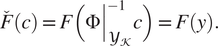 $$ {\left.\overset{\check{}}{F}(c)=F\Big(\Phi \right|}_{{\mathcal{Y}}_{\mathcal{K}}}^{-1}c\Big)=F(y). $$
Further for any $ c\in {\mathcal{V}}_1 $
, we have
$ c\in {\mathcal{V}}_1 $
, we have
 $$ \overset{\check{}}{F}(c)=F\left(\Phi {\left|{}_{{\mathcal{Y}}_{\mathcal{K}}}^{-1}c\left)=F\right(\Phi \right|}_{{\mathcal{Y}}_{\mathcal{K}}}^{-1}V\tilde{c}\right)=F\left({\left.\Phi \right|}_{{\mathcal{Y}}_{\mathcal{K}}}^{-1}\hskip0.1em V{\left({\tilde{c}}_1^T\hskip1em {c}_{R_i}^T{V}_2\hskip1em {\Gamma}^TU\hskip0.1em {\left({S}_{A,2}^{-1}\right)}^T\right)}^T\right)=\tilde{F}\left({\tilde{c}}_1\right). $$
We deduce that $ \tilde{F} $
is actually the restriction of
$ \tilde{F} $
is actually the restriction of $ \overset{\check{}}{F} $
to the subspace
$ \overset{\check{}}{F} $
to the subspace $ {\mathcal{V}}_1 $
.
$ {\mathcal{V}}_1 $
.
From now on, the trajectory $ {y}_{\ast } $
and the associated vector
$ {y}_{\ast } $
and the associated vector $ {c}_{\ast } $
will be considered as random variables and will be denoted by
$ {c}_{\ast } $
will be considered as random variables and will be denoted by $ y $
and
$ y $
and $ c $
. We are interested in the posterior distribution
$ c $
. We are interested in the posterior distribution
 $$ u\left({\tilde{c}}_1\hskip0.1em |\hskip0.1em {\tilde{c}}_{R_1,1},\dots, {\tilde{c}}_{R_I,1}\right), $$
which depends only on the free component $ {\tilde{c}}_1 $
of
$ {\tilde{c}}_1 $
of $ c\in {\mathcal{V}}_1 $
, the two other ones
$ c\in {\mathcal{V}}_1 $
, the two other ones $ {\tilde{c}}_2 $
and
$ {\tilde{c}}_2 $
and $ {\tilde{c}}_3 $
being fixed according to (12). We use Bayes’s rule to model the posterior via the prior and likelihood distributions, leading to
$ {\tilde{c}}_3 $
being fixed according to (12). We use Bayes’s rule to model the posterior via the prior and likelihood distributions, leading to
 $$ u\left({\tilde{c}}_1\hskip0.1em |\hskip0.1em {\tilde{c}}_{R_1,1},\dots, {\tilde{c}}_{R_I,1}\right)\propto u\left({\tilde{c}}_{R_1,1},\dots, {\tilde{c}}_{R_I,1}\hskip0.1em |\hskip0.1em {\tilde{c}}_1\right)\hskip0.1em u\left({\tilde{c}}_1\right). $$
Assuming now that the vectors $ {\tilde{c}}_{R_i,1} $
are independent gives
$ {\tilde{c}}_{R_i,1} $
are independent gives
 $$ u\left({\tilde{c}}_{R_1,1},\dots, {\tilde{c}}_{R_I,1}\hskip0.1em |\hskip0.1em {\tilde{c}}_1\right)\hskip0.1em u\left({\tilde{c}}_1\right)=\prod \limits_{i=1}^Iu\left({\tilde{c}}_{R_i,1}\hskip0.1em |\hskip0.1em {\tilde{c}}_1\right)\hskip0.1em u\left({\tilde{c}}_1\right). $$
The above likelihood is given by the modeling of the reference trajectories detailed in Proposition 3. In this case, we have
 $$ u\left({\tilde{c}}_{R_i,1}\hskip0.1em |\hskip0.1em {\tilde{c}}_1\right)\propto \exp \left(-{\omega}_i{\left({\tilde{c}}_1-{\tilde{c}}_{R_i,1}\right)}^T{\Lambda}_{\Sigma, 1}^{-1}\left({\tilde{c}}_1-{\tilde{c}}_{R_i,1}\right)\right). $$
The prior distribution is obtained by assuming that the most efficient trajectories (with respect to the cost function) are a priori the most likely ones:
 $$ u\left({\tilde{c}}_1\right)\propto \exp \left(-{\kappa}^{-1}\tilde{F}\left({\tilde{c}}_1\right)\right), $$
where $ \kappa >0 $
. Putting everything together and taking the negative of the logarithm gives the following minimization problem, whose solution is the MAP estimator:
$ \kappa >0 $
. Putting everything together and taking the negative of the logarithm gives the following minimization problem, whose solution is the MAP estimator:
 $$ \left\{\begin{array}{l}{\tilde{c}}_1^{\star}\in \arg \hskip0.1em \underset{{\tilde{c}}_1\in {\unicode{x211D}}^{\sigma }}{\min}\tilde{F}\left({\tilde{c}}_1\right)+\kappa \sum \limits_{i=1}^I{\omega}_i\hskip0.1em {\left({\tilde{c}}_1-{\tilde{c}}_{R_i,1}\right)}^T{\Lambda}_{\Sigma, 1}^{-1}\left({\tilde{c}}_1-{\tilde{c}}_{R_i,1}\right),\\ {}{\tilde{c}}_2={V}_2^T{c}_{R_i},\\ {}{\tilde{c}}_3={S}_{A,2}^{-1}\hskip0.1em {U}^T\Gamma .\end{array}\;\right. $$
where $ i $
is arbitrarily chosen in
$ i $
is arbitrarily chosen in $ \left\{1,\dots, I\right\} $
.
$ \left\{1,\dots, I\right\} $
.
Let us now rewrite the above optimization problem with respect to the variable $ c=V\tilde{c}\in {\unicode{x211D}}^K $
in order to make it more interpretable.
$ c=V\tilde{c}\in {\unicode{x211D}}^K $
in order to make it more interpretable.
Proposition 4. The optimization problem (14) is equivalent to the following one:
 $$ {c}^{\star}\in \underset{c\in {\mathcal{V}}_1}{\arg \hskip0.1em \min}\;\overset{\check{}}{F}(c)+\kappa \sum \limits_{i=1}^I{\omega}_i\hskip0.1em {\left(c-{c}_{R_i}\right)}^T{\Sigma}^{\dagger}\left(c-{c}_{R_i}\right), $$
where $ {\Sigma}^{\dagger}\in {\unicode{x211D}}^{K\times K} $
denotes the pseudoinverse of the matrix
$ {\Sigma}^{\dagger}\in {\unicode{x211D}}^{K\times K} $
denotes the pseudoinverse of the matrix $ \Sigma $
.
$ \Sigma $
.
Proof. From (8), we deduce
 $$ {\displaystyle \begin{array}{c}\sum \limits_{i=1}^I{\omega}_i\hskip0.1em {\left({\tilde{c}}_1-{\tilde{c}}_{R_i,1}\right)}^T{\Lambda}_{\Sigma, 1}^{-1}\left({\tilde{c}}_1-{\tilde{c}}_{R_i,1}\right)=\sum \limits_{i=1}^I{\omega}_i\hskip0.1em {\left(\tilde{c}-{\tilde{c}}_{R_i}\right)}^T{\Lambda}_{\Sigma}^{\dagger}\left(\tilde{c}-{\tilde{c}}_{R_i}\right)\\ {}\hskip25em =\sum \limits_{i=1}^I{\omega}_i\hskip0.1em {\left(c-{c}_{R_i}\right)}^T\hskip0.1em V{\Lambda}_{\Sigma}^{\dagger }{V}^T\hskip0.1em \left(c-{c}_{R_i}\right)\\ {}\hskip21.5em =\sum \limits_{i=1}^I{\omega}_i\hskip0.1em {\left(c-{c}_{R_i}\right)}^T{\Sigma}^{\dagger}\left(c-{c}_{R_i}\right).\end{array}} $$
And from the proof of proposition 3, we have
 $$ A\hskip0.1em c=\Gamma \hskip2em \iff \hskip2em {\tilde{c}}_3={S}_{A,2}^{-1}\hskip0.1em {U}^T\Gamma, $$
proving that $ c\in {\mathcal{V}}_1 $
.
$ c\in {\mathcal{V}}_1 $
.
To conclude, let us comment on this optimization problem.
-
1. To interpret the optimization problem (15) (or equivalently (14)) from a geometric point of view, let us consider the following new problem:
(16)
$$ {\displaystyle \begin{array}{ll}& \underset{{\tilde{c}}_1\in {\unicode{x211D}}^{\sigma }}{\min}\tilde{F}\left({\tilde{c}}_1\right)\\ {}\mathrm{s}.\mathrm{t}.& \sum \limits_{i=1}^I{\omega}_i\hskip0.1em {\left({\tilde{c}}_1-{\tilde{c}}_{R_i,1}\right)}^T{\Lambda}_{\Sigma, 1}^{-1}\left({\tilde{c}}_1-{\tilde{c}}_{R_i,1}\right)\leqslant \tilde{\kappa}\end{array}}, $$
where
$ \lambda \geqslant 0 $
. Here, we suppose that
$ \tilde{F} $
is strictly convex and that the problem (16) has a solution (which is then unique). By Slater’s theorem (Boyd and Vandenberghe, Reference Boyd and Vandenberghe2004, Section 5.2.3), the strong duality holds for the problem (16). It can then be proved that there exists a certain
$ {\lambda}^{\star}\geqslant 0 $
such that the solution of (16) is the minimizer of the strictly convex function
$$ {\tilde{c}}_1\mapsto \tilde{F}\left({\tilde{c}}_1\right)+{\lambda}^{\star}\sum \limits_{i=1}^I{\omega}_i\hskip0.1em {\left({\tilde{c}}_1-{\tilde{c}}_{R_i,1}\right)}^T{\Lambda}_{\Sigma, 1}^{-1}\left({\tilde{c}}_1-{\tilde{c}}_{R_i,1}\right), $$
which is actually the objective function of the optimization problem (14) for
$ \kappa ={\lambda}^{\star } $
. Hence, the problem (14) minimizes the cost
$ \tilde{F} $
in a ball centered on the weighted average of the reference trajectories. In particular, if the reference trajectories are close to an optimal one with respect to
$ \tilde{F} $
then one could expect the solution of (14) to be equal to this optimal trajectory. -
2. Further the optimization problem (15) takes into account the endpoints conditions through the subspace
$ {\mathcal{V}}_1 $
but not the additional constraints. However, as explained in the preceding point, the solution is close to realistic trajectories and so is likely to comply with the additional constraints for a well-chosen parameter
$ \kappa >0 $
. We refer to Section 2.6 for more details on an iterative method for the tuning of
$ \kappa $
. In particular, a right choice for this parameter is expected to provide an optimized trajectory with a realistic behavior. This is for instance illustrated in Section 4. -
3. Taking into account the linear information from the available data through the covariance matrix
$ \Sigma $
allows to restrict the search to the subspace
$ {\mathcal{V}}_1 $
describing these relations. This is of particular interest when implicit relations (modeled by the submatrix
$ {V}_2 $
) are revealed by the estimation of
$ \Sigma $
on the basis of the reference trajectories; in this case, these implicit relations may not be known by the expert. -
4. The optimization problem (15) has linear constraints and a quadratic penalized term. For instance, if the cost function
$ \overset{\check{}}{F} $
is a convex function then we obtain a convex problem for which efficient algorithms exist.


2.5. Quadratic cost for a convex optimization problem
In this short subsection, we focus on a particular case where the cost function $ F $
is defined as the integral of an instantaneous quadratic cost function, that is
$ F $
is defined as the integral of an instantaneous quadratic cost function, that is
 $$ \forall y\in \mathcal{C}\left(\left[0,T\right],{\unicode{x211D}}^D\right)\hskip2em F(y)={\int}_0^Tf\left(y(t)\right)\hskip0.1em dt, $$
where $ f:{\unicode{x211D}}^D\to \unicode{x211D} $
is quadratic. Even though such a setting may appear to be restrictive, we emphasize that quadratic models may lead to highly accurate approximations of variables, as it is illustrated in Section 4. For a quadratic instantaneous cost, the associated function
$ f:{\unicode{x211D}}^D\to \unicode{x211D} $
is quadratic. Even though such a setting may appear to be restrictive, we emphasize that quadratic models may lead to highly accurate approximations of variables, as it is illustrated in Section 4. For a quadratic instantaneous cost, the associated function $ \overset{\check{}}{F}:{\unicode{x211D}}^K\to \unicode{x211D} $
can be proved to be quadratic as well and can be explicitly computed. In the following result, we provide a quadratic optimization problem equivalent to (15).
$ \overset{\check{}}{F}:{\unicode{x211D}}^K\to \unicode{x211D} $
can be proved to be quadratic as well and can be explicitly computed. In the following result, we provide a quadratic optimization problem equivalent to (15).
Proposition 5.
Suppose that the cost function $ F $
is of the form (17) with
$ F $
is of the form (17) with $ f $
quadratic. Then the optimization problem (15) is equivalent to the following one:
$ f $
quadratic. Then the optimization problem (15) is equivalent to the following one:
 $$ {c}^{\star}\in \underset{c\in {\mathcal{V}}_1}{\arg \hskip0.1em \min}\;{c}^T\left(\overset{\check{}}{Q}+\kappa \hskip0.1em {\Sigma}^{\dagger}\right)c+{\left(\overset{\check{}}{w}-2\kappa \sum \limits_{i=1}^I{\omega}_i\hskip0.1em {\Sigma}^{\dagger }{c}_{R_i}\right)}^Tc, $$
where $ \overset{\check{}}{Q}\in {\unicode{x211D}}^{K\times K} $
and
$ \overset{\check{}}{Q}\in {\unicode{x211D}}^{K\times K} $
and $ \overset{\check{}}{w}\in {\unicode{x211D}}^K $
can be explicitly computed from
$ \overset{\check{}}{w}\in {\unicode{x211D}}^K $
can be explicitly computed from $ f $
.
$ f $
.
Proof. We defer the proof to Appendix A.
In particular, this allows to derive sufficient conditions on the parameter $ \kappa >0 $
, so that the optimization problem is proved to be equivalent to a quadratic program (Boyd and Vandenberghe, Reference Boyd and Vandenberghe2004, Section 4.4), namely the objective function is convex quadratic together with affine constraints. In practice, this allows to make use of efficient optimization libraries to solve numerically (18).
$ \kappa >0 $
, so that the optimization problem is proved to be equivalent to a quadratic program (Boyd and Vandenberghe, Reference Boyd and Vandenberghe2004, Section 4.4), namely the objective function is convex quadratic together with affine constraints. In practice, this allows to make use of efficient optimization libraries to solve numerically (18).
2.6. Iterative process to comply with additional constraints
As explained in Section 2.4, the trajectory optimization problem (15) is constrained by the endpoints conditions and by implicit linear relations revealed by the reference trajectories. Nevertheless the additional constraints introduced in Definition 3 are not taken into account in this problem. In practice, such constraints assure that natural or user-defined features are verified and so a trajectory which does not comply with these constraints may be considered as unrealistic.
Our aim is then to assure that the trajectory $ {\left.{y}^{\star }=\Phi \right|}_{{\mathcal{Y}}_{\mathcal{K}}}^{-1}{c}^{\star } $
, where
$ {\left.{y}^{\star }=\Phi \right|}_{{\mathcal{Y}}_{\mathcal{K}}}^{-1}{c}^{\star } $
, where $ {c}^{\star}\in {\mathcal{V}}_1 $
is the solution of the optimization problem (15), verifies the additional constraints, that is belongs to the set
$ {c}^{\star}\in {\mathcal{V}}_1 $
is the solution of the optimization problem (15), verifies the additional constraints, that is belongs to the set $ \mathcal{G} $
. A first solution would be to add the constraint
$ \mathcal{G} $
. A first solution would be to add the constraint $ {\left.\Phi \right|}_{{\mathcal{Y}}_{\mathcal{K}}}^{-1}c\in \mathcal{G} $
in the optimization problem (15). However, depending on the nature of the constraints functions
$ {\left.\Phi \right|}_{{\mathcal{Y}}_{\mathcal{K}}}^{-1}c\in \mathcal{G} $
in the optimization problem (15). However, depending on the nature of the constraints functions $ {g}_{\mathrm{\ell}} $
, this may lead to nonlinear constraints which could be costly from a numerical point of view. The solution we propose consists rather in exploiting the degree of freedom coming from the parameter
$ {g}_{\mathrm{\ell}} $
, this may lead to nonlinear constraints which could be costly from a numerical point of view. The solution we propose consists rather in exploiting the degree of freedom coming from the parameter $ \kappa >0 $
appearing in the problem (15).
$ \kappa >0 $
appearing in the problem (15).
First of all, let us factorize the problem (15) by $ \kappa $
to obtain the following new one for the sake of presentation:
$ \kappa $
to obtain the following new one for the sake of presentation:
 $$ {c}^{\star}\in \underset{c\in {\mathcal{V}}_1}{\arg \hskip0.1em \min}\;\nu \hskip0.1em \overset{\check{}}{F}(c)+\sum \limits_{i=1}^I{\omega}_i\hskip0.1em {\left(c-{c}_{R_i}\right)}^T{\Sigma}^{\dagger}\left(c-{c}_{R_i}\right), $$
where $ \nu := {\kappa}^{-1} $
. On one hand, we observe that the solution of the optimization problem (19) for the limit case
$ \nu := {\kappa}^{-1} $
. On one hand, we observe that the solution of the optimization problem (19) for the limit case $ \nu =0 $
is given by
$ \nu =0 $
is given by $ {\sum}_{i=1}^I{\omega}_i\hskip0.1em {c}_{R_i} $
which is the average of the reference vectors. In this case, one may expect that the associated average trajectory complies with the constraints but is unlikely to optimize the cost function
$ {\sum}_{i=1}^I{\omega}_i\hskip0.1em {c}_{R_i} $
which is the average of the reference vectors. In this case, one may expect that the associated average trajectory complies with the constraints but is unlikely to optimize the cost function $ F $
. On the other hand, for very large
$ F $
. On the other hand, for very large $ \nu >0 $
, the second term of the objective function in (19) can be considered as negligible compared to the first one. In this case, the cost of the solution will surely be smaller than the costs of the reference trajectories but no guarantee regarding the additional constraints can be established in a general setting.
$ \nu >0 $
, the second term of the objective function in (19) can be considered as negligible compared to the first one. In this case, the cost of the solution will surely be smaller than the costs of the reference trajectories but no guarantee regarding the additional constraints can be established in a general setting.
Given these observations, the task is then to find an appropriate value $ {\nu}^{\star }>0 $
in order to reach a trade-off between optimizing and remaining close to the reference trajectories to comply with the additional constraints. Many methods can be developed to find such a
$ {\nu}^{\star }>0 $
in order to reach a trade-off between optimizing and remaining close to the reference trajectories to comply with the additional constraints. Many methods can be developed to find such a $ {\nu}^{\star } $
but here we propose a very simple one based on a binary search algorithm. We exploit the assumption that the solution for
$ {\nu}^{\star } $
but here we propose a very simple one based on a binary search algorithm. We exploit the assumption that the solution for $ \nu =0 $
(i.e., the reference trajectories average) is admissible. We proceed then as follows:
$ \nu =0 $
(i.e., the reference trajectories average) is admissible. We proceed then as follows:
-
1. We set firstly a maximal value
$ {\nu}_{max}>0 $
so that the solution of (19) with
$ {\nu}_{max} $
does not satisfy the constraints. For instance, we choose a large value, solve the optimization problem and check the constraints. If they are still satisfied, we choose a larger
$ {\nu}_{max} $
. -
2. Then apply a binary search between
$ 0 $
and
$ {\nu}_{max} $
: solve the optimization problem for
$ \frac{\nu_{max}}{2} $
; if the resulting solution verifies the constraints, solve the problem again for
$ \frac{3{\nu}_{max}}{4} $
; else solve it for
$ \frac{\nu_{max}}{4} $
. -
3. Continue the process until a user-defined stopping criterion.


Other iterative processes can also be considered.
2.7. Confidence bounds on the integrated cost
In practice the cost function $ F $
considered is an estimation of the true cost
$ F $
considered is an estimation of the true cost $ {F}^{\star } $
, a random variable which cannot be fully predicted based on
$ {F}^{\star } $
, a random variable which cannot be fully predicted based on $ y $
. If the distribution
$ y $
. If the distribution $ F(y) $
was known we could deduce a confidence bound on
$ F(y) $
was known we could deduce a confidence bound on $ {F}^{\star } $
. This is for instance possible by considering multivariate functional regression Ramsay et al. (Reference Ramsay, Hooker, Campbell and Cao2007).
$ {F}^{\star } $
. This is for instance possible by considering multivariate functional regression Ramsay et al. (Reference Ramsay, Hooker, Campbell and Cao2007).
The simplest case from the estimation point of view is to consider that $ {F}^{\star } $
is the integral of some instantaneous consumption function
$ {F}^{\star } $
is the integral of some instantaneous consumption function $ {f}^{\star } $
as in Section 2.5, and to estimate the parameters of the standard multivariate regression
$ {f}^{\star } $
as in Section 2.5, and to estimate the parameters of the standard multivariate regression
 $$ {f}^{\star}\left(y(t)\right)=f\left(y(t)\right)+\varepsilon (t), $$
where the random noise $ \varepsilon (t) $
is assumed to follow a centered Gaussian distribution with variance
$ \varepsilon (t) $
is assumed to follow a centered Gaussian distribution with variance $ \sigma $
. In this case,
$ \sigma $
. In this case, $ {F}^{\star } $
can be expressed as the integral of a stochastic process
$ {F}^{\star } $
can be expressed as the integral of a stochastic process
 $$ {F}^{\star }(y):= {\int}_0^T{f}^{\star}\left(y(t)\right)\hskip0.1em dt=F(y)+{\int}_0^T\varepsilon (t)\hskip0.1em dt, $$
then assuming that $ {\left(\varepsilon (t)\right)}_{t\in \left[0,T\right]} $
independent, we obtain
$ {\left(\varepsilon (t)\right)}_{t\in \left[0,T\right]} $
independent, we obtain
 $$ {\int}_0^T\varepsilon (t)\hskip0.1em dt\sim \mathcal{N}\left(0,T{\sigma}^2\right). $$
Thus $ {F}^{\star }(y) $
follows a Gaussian distribution centered on
$ {F}^{\star }(y) $
follows a Gaussian distribution centered on $ F(y) $
and with variance equals to
$ F(y) $
and with variance equals to $ T{\sigma}^2 $
. This makes it possible to compute confidence bounds on
$ T{\sigma}^2 $
. This makes it possible to compute confidence bounds on $ {F}^{\star }(y) $
. For a confidence level
$ {F}^{\star }(y) $
. For a confidence level $ 1-u $
,
$ 1-u $
, $ u\in \left[0,1\right] $
, a confidence interval for
$ u\in \left[0,1\right] $
, a confidence interval for $ {F}^{\star }(y) $
is obtained as
$ {F}^{\star }(y) $
is obtained as
 $$ {\mathtt{CI}}^{1-u}\left({F}^{\star }(y)\right)=F(y)\pm {\zeta}_{1-\frac{u}{2}}\sqrt{T}\sigma, $$
where $ {\zeta}_{1-\frac{u}{2}} $
is the quantile of order
$ {\zeta}_{1-\frac{u}{2}} $
is the quantile of order $ 1-\frac{u}{2} $
of the standard Gaussian distribution.
$ 1-\frac{u}{2} $
of the standard Gaussian distribution.
The assumption that $ f $
and
$ f $
and $ {\sigma}^2 $
are known is relevant since they are estimated based on a huge amount of training data. The assumption of white Gaussian noise can be seen as unrealistic, however, it appears to be the only route to explicit calculus. A more complex strategy could be derived using Gaussian processes, which is beyond the scope of this paper.
$ {\sigma}^2 $
are known is relevant since they are estimated based on a huge amount of training data. The assumption of white Gaussian noise can be seen as unrealistic, however, it appears to be the only route to explicit calculus. A more complex strategy could be derived using Gaussian processes, which is beyond the scope of this paper.
3. The Python Library Pyrotor
The above optimization methodology is aimed at being used in a wide range of applications, from path planning for industrial robots (Chettibi et al., Reference Chettibi, Lehtihet, Haddad and Hanchi2004) to fuel-efficient aircraft trajectories (Rommel et al., Reference Rommel, Bonnans, Martinon and Gregorutti2019; Dewez et al., Reference Dewez, Guedj and Vandewalle2020). We therefore contribute a generic Python library PyRotor (standing for Python Route trajectory optimizer) which is intended to the largest audience. PyRotor is the backbone to numerical results given in this paper.
When using the PyRotor library, the practitioner has to define the endpoints conditions as a dictionary, the additional constraints in a list of functions, the name of the basis and the dimension for each variable. The current version of the library covers only the case of Section 2.5, that is to say the cost is given by a quadratic instantaneous function. This permits to make use of Proposition 5 in which a quadratic objective function is given. We mention that future releases of PyRotor are intended to cover more general cost functions. The value of the parameter $ {\nu}_{max} $
in (19) can also be manually set depending on the application. The Legendre basis and B-splines are currently the bases implemented in the first version of PyRotor (via the legendre module from NumPy package Harris et al., Reference Harris, Millman, van der Walt, Gommers, Virtanen, Cournapeau, Wieser, Taylor, Berg, Smith, Kern, Picus, Hoyer, van Kerkwijk, Brett, Haldane, Fernández del Río, Wiebe, Peterson, Gérard-Marchant, Sheppard, Reddy, Weckesser, Abbasi, Gohlke and Oliphant2020 and the interpolate module from Scipy package Virtanen et al., Reference Virtanen, Gommers, Oliphant, Haberland, Reddy, Cournapeau, Burovski, Peterson, Weckesser, Bright, van der Walt, Brett, Wilson, Millman, Mayorov, Nelson, Jones, Kern, Larson, Carey, Polat, Feng, Moore, VanderPlas, Laxalde, Perktold, Cimrman, Henriksen, Quintero, Harris, Archibald, Ribeiro, Pedregosa and van Mulbregt2020) but future developments including other general bases are planned. Further, the user indicates a path to a directory containing the data, each reference trajectory being contained in a csv file. The covariance matrix
$ {\nu}_{max} $
in (19) can also be manually set depending on the application. The Legendre basis and B-splines are currently the bases implemented in the first version of PyRotor (via the legendre module from NumPy package Harris et al., Reference Harris, Millman, van der Walt, Gommers, Virtanen, Cournapeau, Wieser, Taylor, Berg, Smith, Kern, Picus, Hoyer, van Kerkwijk, Brett, Haldane, Fernández del Río, Wiebe, Peterson, Gérard-Marchant, Sheppard, Reddy, Weckesser, Abbasi, Gohlke and Oliphant2020 and the interpolate module from Scipy package Virtanen et al., Reference Virtanen, Gommers, Oliphant, Haberland, Reddy, Cournapeau, Burovski, Peterson, Weckesser, Bright, van der Walt, Brett, Wilson, Millman, Mayorov, Nelson, Jones, Kern, Larson, Carey, Polat, Feng, Moore, VanderPlas, Laxalde, Perktold, Cimrman, Henriksen, Quintero, Harris, Archibald, Ribeiro, Pedregosa and van Mulbregt2020) but future developments including other general bases are planned. Further, the user indicates a path to a directory containing the data, each reference trajectory being contained in a csv file. The covariance matrix $ \Sigma $
is here estimated by using the sklearn.covariance package from the Python library scikit-learn (Pedregosa et al., Reference Pedregosa, Varoquaux, Gramfort, Michel, Thirion, Grisel, Blondel, Prettenhofer, Weiss, Dubourg, Vanderplas, Passos, Cournapeau, Brucher, Perrot and Duchesnay2011). Two optimization solvers are proposed: the generic solver minimize(method=’trust-constr’; Conn et al., Reference Conn, Gould and Toint2000) from SciPy and the quadratic programming solver from CVXOPT software (Andersen et al., Reference Andersen, Dahl and Vandenberghe2020). The latter is intended to speed up the execution in case of convex quadratic objective function. Once the arguments are given by the user, a class is created and the optimization is performed by executing a method from this class. At the end, the optimized trajectory is provided in a dataframe: at each time, the position of the trajectory is given together with the value of
$ \Sigma $
is here estimated by using the sklearn.covariance package from the Python library scikit-learn (Pedregosa et al., Reference Pedregosa, Varoquaux, Gramfort, Michel, Thirion, Grisel, Blondel, Prettenhofer, Weiss, Dubourg, Vanderplas, Passos, Cournapeau, Brucher, Perrot and Duchesnay2011). Two optimization solvers are proposed: the generic solver minimize(method=’trust-constr’; Conn et al., Reference Conn, Gould and Toint2000) from SciPy and the quadratic programming solver from CVXOPT software (Andersen et al., Reference Andersen, Dahl and Vandenberghe2020). The latter is intended to speed up the execution in case of convex quadratic objective function. Once the arguments are given by the user, a class is created and the optimization is performed by executing a method from this class. At the end, the optimized trajectory is provided in a dataframe: at each time, the position of the trajectory is given together with the value of $ f $
. The total cost is also computed and a quantitative comparison in terms of savings with the reference trajectories can be also displayed.
$ f $
. The total cost is also computed and a quantitative comparison in terms of savings with the reference trajectories can be also displayed.
The open source PyRotor library is developed on GitHub and welcomes contributions from its users: we favor a community-based development to foster the diffusion of our work toward practitioners. PyRotor is intended to be PEP8 compliant and purposely rely on high standard coding practices. The continuous development platform Travis is used to certify the latest builds of the library. Finally, we provide Jupyter notebooks, for example, on how to use PyRotor along with online documentation. PyRotor is available at https://github.com/bguedj/pyrotor.
4. Application 1: Trajectory Optimization for Fuel-Efficient Aircrafts
In this section, we consider the aeronautic problem of reducing the total fuel consumption of an aircraft during the climb phase. This example illustrates the key role played by the reference trajectories since we are able to obtain optimized trajectories with realistic patterns thanks to a simple modeling involving few constraints.
4.1. Modeling
Here, the trajectories are supposed to be in a vertical plane and are defined by the altitude $ h $
, the Mach number
$ h $
, the Mach number $ \mathrm{M} $
and the engines rotational speed
$ \mathrm{M} $
and the engines rotational speed $ \mathrm{N}1 $
(expressed as a percentage of a maximal value). Hence, a trajectory
$ \mathrm{N}1 $
(expressed as a percentage of a maximal value). Hence, a trajectory $ y $
in this setting is a continuous
$ y $
in this setting is a continuous $ {\unicode{x211D}}^3 $
-valued map defined on
$ {\unicode{x211D}}^3 $
-valued map defined on $ \left[0,T\right] $
, where
$ \left[0,T\right] $
, where $ T $
is a maximal climb duration fixed by the user. Hence, we have
$ T $
is a maximal climb duration fixed by the user. Hence, we have
 $$ \forall t\in \left[0,T\right]\hskip2em y(t):= \left(h(t),\mathrm{M}(t),\mathrm{N}1(t)\right). $$
The quantity to minimize is the total fuel consumption $ \mathrm{TFC}:\mathcal{C}\left(\left[0,T\right],{\unicode{x211D}}^3\right)\to {\unicode{x211D}}_{+} $
which is defined via the fuel flow
$ \mathrm{TFC}:\mathcal{C}\left(\left[0,T\right],{\unicode{x211D}}^3\right)\to {\unicode{x211D}}_{+} $
which is defined via the fuel flow $ \mathrm{FF}:{\unicode{x211D}}^3\to {\unicode{x211D}}_{+} $
as followsFootnote
4:
$ \mathrm{FF}:{\unicode{x211D}}^3\to {\unicode{x211D}}_{+} $
as followsFootnote
4:
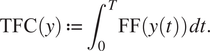 $$ \mathrm{TFC}(y):= {\int}_0^T\mathrm{FF}\left(y(t)\right)\hskip0.1em dt. $$
Regarding the endpoints conditions, we require the trajectory to start at the altitude $ {h}_0 $
with Mach number
$ {h}_0 $
with Mach number $ {\mathrm{M}}_0 $
and to end at the altitude
$ {\mathrm{M}}_0 $
and to end at the altitude $ {h}_T $
with Mach number
$ {h}_T $
with Mach number $ {\mathrm{M}}_T $
. In particular, the reference trajectories we use have to verify these conditions.
$ {\mathrm{M}}_T $
. In particular, the reference trajectories we use have to verify these conditions.
We consider also additional constraints which are conventional in the aeronautic setting:
-
• The rate of climb, that is the time-derivative of the altitude, has to be upper bounded by a given maximal value
$ {\gamma}_{max} $
during the whole climb; -
• The Mach number should not exceed a certain value called the maximum operational Mach (
$ \mathrm{MMO} $
).


The final time of the climb is given by $ {T}^{\star}\in \left[0,T\right] $
which is the first time where the aircraft reaches
$ {T}^{\star}\in \left[0,T\right] $
which is the first time where the aircraft reaches $ {h}_T $
with Mach number
$ {h}_T $
with Mach number $ {\mathrm{M}}_T $
.
$ {\mathrm{M}}_T $
.
Finally, we mention that the fuel flow model $ \mathrm{FF} $
is here estimated. To do so, we exploit the reference trajectories which contain recorded altitude, Mach number, engines power and fuel flow for each second of the flight. Having access to these data, we are in position to fit a statistical model. Following the numerical results in Dewez et al. (Reference Dewez, Guedj and Vandewalle2020) which show that polynomials can accurately model aeronautic variables, we consider a polynomial model of degree 2 for the fuel flow. In particular, the requirements for the cost function in the current version of PyRotor are fulfilled. The prediction accuracy of the resulting estimated model is assessed in the following subsection.
$ \mathrm{FF} $
is here estimated. To do so, we exploit the reference trajectories which contain recorded altitude, Mach number, engines power and fuel flow for each second of the flight. Having access to these data, we are in position to fit a statistical model. Following the numerical results in Dewez et al. (Reference Dewez, Guedj and Vandewalle2020) which show that polynomials can accurately model aeronautic variables, we consider a polynomial model of degree 2 for the fuel flow. In particular, the requirements for the cost function in the current version of PyRotor are fulfilled. The prediction accuracy of the resulting estimated model is assessed in the following subsection.
4.2. Numerical results
We present now numerical results based on real flight data for the above aeronautic problem. Here, we have access to 2,162 recorded short and medium-haul flights performed by the same narrow-body airliner type, provided by a partner airline. In particular they cannot be publicly released for commercial reasons. The data is here recorded by the quick access recorder (QAR).
Before considering the optimization setting, we estimate a fuel flow model specific to the climb phase and to the considered airliner type. To do so, we extract the signals of the four variables of interest (altitude, Mach number, engines rotational speed, and fuel flow) and keep the observations from the take-off to the beginning of the cruise without level-off phases. Smoothing splines are then applied to the raw signals to remove the noise. We sample each 5 s to reduce the dataset size without impacting strongly the accuracy of the resulting models. At the end, we obtain 494,039 observations which are randomly split into training and test sets to fit a polynomial model of degree 2 using the scikit-learn library. The RMSE and MAPE values of this model on the test set are respectively equal to $ 3.64\times {10}^{-2} $
kg/s and 1.73%.
$ 3.64\times {10}^{-2} $
kg/s and 1.73%.
Regarding the optimization, we are interested in climb phases from 3,000 to 38,000 ft. We mention that we remove lower altitudes because operational procedures constraint heavily the trajectory during the very beginning of the climb. Further the initial and final Mach numbers are required to be equal to 0.3 and 0.78. It is noteworthy that the optimization solvers used in PyRotor allow linear inequality conditions, permitting to slightly relax the endpoints conditions. Here we tolerate an error of 100 ft for the altitude and an error of 0.01 for the Mach number. The initial and final $ \mathrm{N}1 $
values are let unconstrained. Finally the
$ \mathrm{N}1 $
values are let unconstrained. Finally the $ \mathrm{MMO} $
and
$ \mathrm{MMO} $
and $ {\gamma}_{max} $
are respectively set to 0.82 and 3,600 ft/min.
$ {\gamma}_{max} $
are respectively set to 0.82 and 3,600 ft/min.
The reference trajectories are given by 48 recorded flights which satisfy the above climb endpoints conditions among the 2,162 available ones. All these selected flights are used to estimate the covariance matrix involved in the optimization problem. On the other hand, we use only the five most fuel-efficient flights in the objective function to focus on a domain containing the most efficient recorded flights. Further the maximal duration $ T $
is here fixed to the duration of the longest climb among the five most fuel-efficient ones we use.
$ T $
is here fixed to the duration of the longest climb among the five most fuel-efficient ones we use.
Legendre polynomials are used as the functional basis spanning the space in which lies the trajectories. Since we consider narrow-body airliners, polynomials are expected to be relevant to describe the slow variations of such aircrafts. Here the dimensions associated with the altitude, the Mach number and the engines power are given respectively by 4, 10, and 6. The reference vectors $ {c}_{R_i} $
are then computed using the formula (2). At the end, we amount to solving a constrained optimization problem in a space of dimension 20.
$ {c}_{R_i} $
are then computed using the formula (2). At the end, we amount to solving a constrained optimization problem in a space of dimension 20.
We are then in position to apply the optimization method developed in Section 2 using the PyRotor library. First of all a relevant value for $ {\nu}_{max}>0 $
has to be fixed. In order to propose a realistic optimized climb, we choose a
$ {\nu}_{max}>0 $
has to be fixed. In order to propose a realistic optimized climb, we choose a $ {\nu}_{max} $
relatively small so that the optimized climb remains close to the reference ones. In particular, the quadratic objective function in (19) turns out to be convex for all
$ {\nu}_{max} $
relatively small so that the optimized climb remains close to the reference ones. In particular, the quadratic objective function in (19) turns out to be convex for all $ \nu \in \left[0,{\nu}_{max}\right] $
permitting to use the quadratic programming solver from CVXOPT software imported in PyRotor. The preprocessing of the reference trajectories and the optimization steps have been executed 100 times using PyRotor on an Intel Core i7 6 cores running at 2.2 GHz. The mean of the execution time for both steps is equal to 3.76 s with standard deviation 0.11 s, illustrating that the library is time-efficient in this setting.
$ \nu \in \left[0,{\nu}_{max}\right] $
permitting to use the quadratic programming solver from CVXOPT software imported in PyRotor. The preprocessing of the reference trajectories and the optimization steps have been executed 100 times using PyRotor on an Intel Core i7 6 cores running at 2.2 GHz. The mean of the execution time for both steps is equal to 3.76 s with standard deviation 0.11 s, illustrating that the library is time-efficient in this setting.
A plot of the optimized trajectory obtained using PyRotor is given in Figure 3. We observe that the optimized trajectory seeks to reach the maximum altitude in the minimum amount of time; this is in accordance with the existing literature (see, for instance, Codina and Menéndez, Reference Codina and Menéndez2014 and references therein). In particular, the duration $ {T}^{\star } $
is equal to 1,033 s which is actually slightly shorter than the reference durations. We note also that the optimized Mach number shares a very similar pattern with the references. On the other hand, the optimized engines rotational speed tends to slowly decrease until the cruise regime before reaching the top of climb. This is not the case for the reference engines speed which falls to the cruise regime just after reaching the final altitude. Most of the savings seem to be achieved in these last moments of the climb. At last but not least, the optimized trajectory presents a realistic pattern inherited from the reference trajectories.
$ {T}^{\star } $
is equal to 1,033 s which is actually slightly shorter than the reference durations. We note also that the optimized Mach number shares a very similar pattern with the references. On the other hand, the optimized engines rotational speed tends to slowly decrease until the cruise regime before reaching the top of climb. This is not the case for the reference engines speed which falls to the cruise regime just after reaching the final altitude. Most of the savings seem to be achieved in these last moments of the climb. At last but not least, the optimized trajectory presents a realistic pattern inherited from the reference trajectories.
Optimized and reference altitudes, Mach numbers and engines rotational speeds—the optimized trajectory is represented by the blue curves.
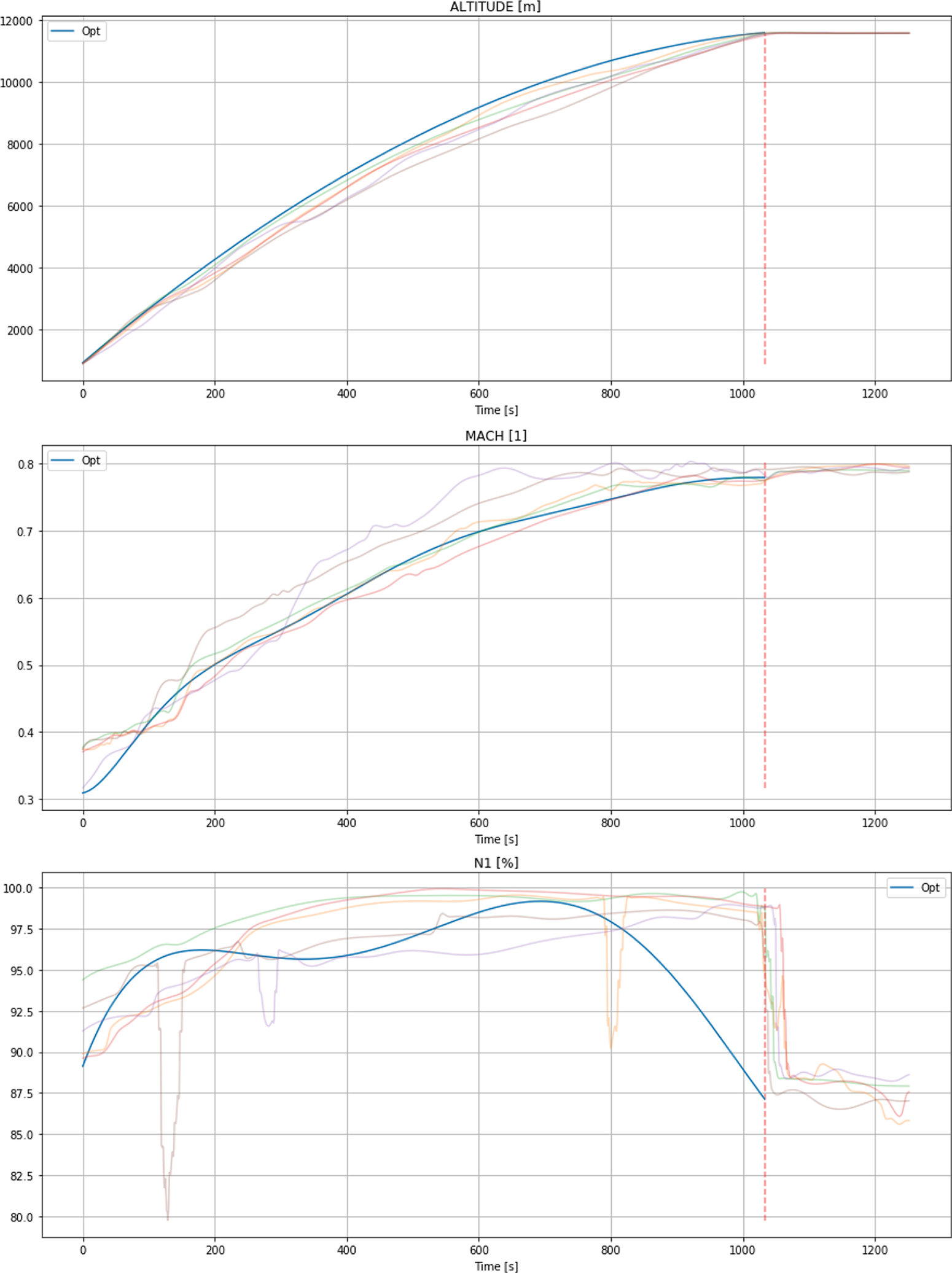
For a quantitative comparison, we refer to Table 1 which provides statistical information on the fuel savings. The mean savings 16.54% together with the fact that the optimized trajectory verifies the additional constraints show that these first results are promising, motivating further studies. For instance one could model environmental conditions or take into account Air Traffic Control constraints for more realistic modelings. In particular, the minimal percentage indicates the savings compared with the best trajectory (i.e., with the lowest consumption).
Statistical description of the fuel savings of the optimized trajectory.
The savings are compared with the 48 recorded flights satisfying the present endpoints and the total consumption of the optimized trajectory is estimated sing the statistical model for the fuel flow. Q 1, Q 2, and Q 3 refer to the first, second and third quartiles.
5. Application 2: Trajectory Optimization to Maximize Work of a Force Field
Here, we consider the following generic example: given a moving point in a force field, find a trajectory starting and ending at two different given points which maximizes the work of the force along the trajectory while minimizing the travelled distance. For instance, this corresponds to a very simple modeling of a sailing boat which seeks to increase the power of the wind at each time, that is maximizing the wind work, without traveling a too large distance. This second example demonstrates that our generic optimization approach is flexible enough to take into account derivatives of trajectories and hence to cover dynamics settings.
5.1. Modeling
To model this problem, we suppose without loss of generality that the trajectories are defined on the (time-) interval $ \left[0,1\right] $
and we let
$ \left[0,1\right] $
and we let $ V:{\unicode{x211D}}^D\to {\unicode{x211D}}^D $
denote a vector field. Furthermore, the trajectories are assumed here to be continuously differentiable, that is they belong to
$ V:{\unicode{x211D}}^D\to {\unicode{x211D}}^D $
denote a vector field. Furthermore, the trajectories are assumed here to be continuously differentiable, that is they belong to $ {\mathcal{C}}^1\left(\left[0,1\right],{\unicode{x211D}}^D\right) $
. The work of
$ {\mathcal{C}}^1\left(\left[0,1\right],{\unicode{x211D}}^D\right) $
. The work of $ V $
along a trajectory
$ V $
along a trajectory $ y\in {\mathcal{C}}^1\left(\left[0,1\right],{\unicode{x211D}}^D\right) $
is
$ y\in {\mathcal{C}}^1\left(\left[0,1\right],{\unicode{x211D}}^D\right) $
is
 $$ W\left(y,\dot{y}\right):= {\int}_0^1V{\left(y(t)\right)}^T\dot{y}(t)\hskip0.1em dt; $$
here $ \dot{y} $
denotes the derivative of
$ \dot{y} $
denotes the derivative of $ y $
with respect to the independent variable
$ y $
with respect to the independent variable $ t $
. Moreover, using Hamilton’s principle in Lagrangian mechanics, it can be shown that the trajectory with constant velocity (i.e., a straight line travelled at constant speed) is the minimum of the following functional,
$ t $
. Moreover, using Hamilton’s principle in Lagrangian mechanics, it can be shown that the trajectory with constant velocity (i.e., a straight line travelled at constant speed) is the minimum of the following functional,
 $$ J\left(\dot{y}\right)={\int}_0^1\parallel \dot{y}(t){\parallel}_2^2\hskip0.1em dt, $$
where the starting and ending points of $ y $
are fixed and different. This functional can be then used to control the travelled distance. It follows that minimizing the cost function
$ y $
are fixed and different. This functional can be then used to control the travelled distance. It follows that minimizing the cost function
 $$ {F}_{\alpha}\left(y,\dot{y}\right):= \alpha J\left(\dot{y}\right)-W\left(y,\dot{y}\right)={\int}_0^1\alpha \parallel \dot{y}(t){\parallel}_2^2-V{\left(y(t)\right)}^T\dot{y}(t)\hskip0.1em dt, $$
where $ \alpha \geqslant 0 $
is arbitrarily chosen, is expected to lead to an optimized trajectory reflecting a trade-off between maximizing the work and minimizing the distance. Further we require the trajectory to stay in the hypercube
$ \alpha \geqslant 0 $
is arbitrarily chosen, is expected to lead to an optimized trajectory reflecting a trade-off between maximizing the work and minimizing the distance. Further we require the trajectory to stay in the hypercube $ {\left[0,1\right]}^D $
and to start and to end respectively at
$ {\left[0,1\right]}^D $
and to start and to end respectively at $ {y}_0\in {\left[0,1\right]}^D $
and
$ {y}_0\in {\left[0,1\right]}^D $
and $ {y}_1\in {\left[0,1\right]}^D $
.
$ {y}_1\in {\left[0,1\right]}^D $
.
Now, we remark that the above cost function involves the (time-)derivative $ \dot{y} $
. So one has to derive a formula permitting to compute the derivative of any trajectory
$ \dot{y} $
. So one has to derive a formula permitting to compute the derivative of any trajectory $ {\left.y=\Phi \right|}_{{\mathcal{Y}}_{\mathcal{K}}}^{-1}c\in {\mathcal{Y}}_{\mathcal{K}} $
from its associated vector
$ {\left.y=\Phi \right|}_{{\mathcal{Y}}_{\mathcal{K}}}^{-1}c\in {\mathcal{Y}}_{\mathcal{K}} $
from its associated vector $ c\in {\unicode{x211D}}^K $
, especially to compute
$ c\in {\unicode{x211D}}^K $
, especially to compute $ \overset{\check{}}{F}(c) $
. For instance, this can be easily achieved by assuming that each element of the functional basis is continuously differentiable. Indeed we can differentiate in this case any
$ \overset{\check{}}{F}(c) $
. For instance, this can be easily achieved by assuming that each element of the functional basis is continuously differentiable. Indeed we can differentiate in this case any $ y\in {\mathcal{Y}}_{\mathcal{K}} $
:
$ y\in {\mathcal{Y}}_{\mathcal{K}} $
:
 $$ \forall d=1,\dots, D\hskip2em {\dot{y}}^{(d)}=\sum \limits_{k=1}^{K_d}{c}_k^{(d)}{\dot{\varphi}}_k={\left({\left.\frac{d}{dt}\Phi \right|}_{{\mathcal{Y}}_{\mathcal{K}}}^{-1}c\right)}^{(d)}. $$
We deduce then the following formula for $ \overset{\check{}}{F}(c) $
in the present setting:
$ \overset{\check{}}{F}(c) $
in the present setting:
 $$ \overset{\check{}}{F}(c):= {F}_{\alpha}\left(\Phi {\left|{}_{{\mathcal{Y}}_{\mathcal{K}}}^{-1}c,\frac{d}{dt}\Phi \right|}_{{\mathcal{Y}}_{\mathcal{K}}}^{-1}c\right). $$
Here, the vector $ c $
contains information on both position and velocity, permitting especially to keep the problem dimension unchanged. To finish, let us remark that it is possible to make the above formula for
$ c $
contains information on both position and velocity, permitting especially to keep the problem dimension unchanged. To finish, let us remark that it is possible to make the above formula for $ \overset{\check{}}{F} $
explicit with respect to
$ \overset{\check{}}{F} $
explicit with respect to $ c $
in certain settings. For instance it is possible to derive an explicit quadratic formula for
$ c $
in certain settings. For instance it is possible to derive an explicit quadratic formula for $ \overset{\check{}}{F}(c) $
when the integrand defining
$ \overset{\check{}}{F}(c) $
when the integrand defining $ {F}_{\alpha } $
is quadratic with respect to
$ {F}_{\alpha } $
is quadratic with respect to $ y(t) $
and
$ y(t) $
and $ \dot{y}(t) $
; this formula is implemented in PyRotor and the arguments to obtain it are similar to those proving Proposition 5.
$ \dot{y}(t) $
; this formula is implemented in PyRotor and the arguments to obtain it are similar to those proving Proposition 5.
5.2. Numerical results
Numerical results based on randomly generated data for the above physical application are presented in this section. We first consider trajectories with two components $ {y}^{(1)} $
and
$ {y}^{(1)} $
and $ {y}^{(2)} $
lying in the square
$ {y}^{(2)} $
lying in the square $ {\left[0,1\right]}^2 $
for the sake of simplicity. We set the starting and ending points as follows:
$ {\left[0,1\right]}^2 $
for the sake of simplicity. We set the starting and ending points as follows:
 $$ {y}^{(1)}(0)=0.111\hskip1em ,\hskip1em {y}^{(2)}(0)=0.926\hskip1em ,\hskip1em {y}^{(1)}(1)=0.912\hskip1em ,\hskip1em {y}^{(2)}(1)=0.211 $$
with a tolerated error $ 1\times {10}^{-4} $
, and the vector field
$ 1\times {10}^{-4} $
, and the vector field $ V:{\unicode{x211D}}^2\to {\unicode{x211D}}^2 $
is here defined by
$ V:{\unicode{x211D}}^2\to {\unicode{x211D}}^2 $
is here defined by
 $$ V\left({x}^{(1)},{x}^{(2)}\right)={\left(0,{x}^{(1)}\right)}^T. $$
Given the above endpoints and the vector field, we observe that the force modelled by $ V $
will be in average a resistance force to the motion. Indeed the force is oriented toward the top of the square while the moving point has to go downward. Further, let us note that the integrand of the cost function
$ V $
will be in average a resistance force to the motion. Indeed the force is oriented toward the top of the square while the moving point has to go downward. Further, let us note that the integrand of the cost function $ {F}_{\alpha } $
in the present setting is actually quadratic with respect to
$ {F}_{\alpha } $
in the present setting is actually quadratic with respect to $ y(t) $
and
$ y(t) $
and $ \dot{y}(t) $
, so that an explicit quadratic formula for
$ \dot{y}(t) $
, so that an explicit quadratic formula for $ \overset{\check{}}{F}(c) $
implemented in PyRotor is available.
$ \overset{\check{}}{F}(c) $
implemented in PyRotor is available.
Here, the reference trajectories are obtained through a random generation process. To do so, we define an arbitrarily trajectory $ {y}_R $
verifying the endpoints conditions and we compute its associated vector
$ {y}_R $
verifying the endpoints conditions and we compute its associated vector $ {c}_R $
; Legendre polynomials are once again used and the dimensions of
$ {c}_R $
; Legendre polynomials are once again used and the dimensions of $ {y}^{(1)} $
and
$ {y}^{(1)} $
and $ {y}^{(2)} $
are here set to 4 and 6. Let us note that
$ {y}^{(2)} $
are here set to 4 and 6. Let us note that $ {y}_R $
is designed in such a way that it has a relevant pattern but not the optimal one. Then we construct a set of reference trajectories by adding centered Gaussian noises to
$ {y}_R $
is designed in such a way that it has a relevant pattern but not the optimal one. Then we construct a set of reference trajectories by adding centered Gaussian noises to $ {c}_R $
. It is noteworthy that the noise is generated in such a way that it belongs to the null space of the matrix
$ {c}_R $
. It is noteworthy that the noise is generated in such a way that it belongs to the null space of the matrix $ A $
describing the endpoints conditions; the resulting noised trajectories satisfy then these conditions. Further the trajectories which go out of the square
$ A $
describing the endpoints conditions; the resulting noised trajectories satisfy then these conditions. Further the trajectories which go out of the square $ {\left[0,1\right]}^2 $
are not kept. At the end, we get 122 generated reference trajectories assumed to be realistic in this setting, each of them containing 81 time observations. Among these reference trajectories, we use the 10 most efficient ones with respect to the cost
$ {\left[0,1\right]}^2 $
are not kept. At the end, we get 122 generated reference trajectories assumed to be realistic in this setting, each of them containing 81 time observations. Among these reference trajectories, we use the 10 most efficient ones with respect to the cost $ {F}_{\alpha } $
.
$ {F}_{\alpha } $
.
In the present example, we set a $ {\nu}_{max} $
relatively large to explore a large domain around the reference trajectories. In this case, the objective function of the optimization problem (19) may be not convex even if it is still quadratic. So we make use of the generic optimization solver minimize(method=’trust-constr’) imported in PyRotor. Regarding the execution time, we have randomly and uniformly generated 100 values in the interval
$ {\nu}_{max} $
relatively large to explore a large domain around the reference trajectories. In this case, the objective function of the optimization problem (19) may be not convex even if it is still quadratic. So we make use of the generic optimization solver minimize(method=’trust-constr’) imported in PyRotor. Regarding the execution time, we have randomly and uniformly generated 100 values in the interval $ \left[0,10\right] $
for the parameter
$ \left[0,10\right] $
for the parameter $ \alpha $
and executed PyRotor for each of them. The mean of PyRotor execution time is 0.44 s with standard deviation 0.03 s on an Intel Core i7 6 cores running at 2.2 GHz.
$ \alpha $
and executed PyRotor for each of them. The mean of PyRotor execution time is 0.44 s with standard deviation 0.03 s on an Intel Core i7 6 cores running at 2.2 GHz.
In Figure 4, we plot four optimized trajectories associated with different values of $ \alpha $
: 0, 0.35, 1, and 10. As expected the trajectory associated with the largest value of
$ \alpha $
: 0, 0.35, 1, and 10. As expected the trajectory associated with the largest value of $ \alpha $
gives the most straight trajectory while the most curvy one is associated with
$ \alpha $
gives the most straight trajectory while the most curvy one is associated with $ \alpha =0 $
. In particular, the latter tends to move to the left at the beginning where the force
$ \alpha =0 $
. In particular, the latter tends to move to the left at the beginning where the force $ V $
is the smallest before going to the ending point in a quasi-straightforward way so that the force is perpendicular to the motion. This example illustrates especially that our optimization approach may lead to optimized trajectories which slightly differ from the reference ones to reduce more the cost.
$ V $
is the smallest before going to the ending point in a quasi-straightforward way so that the force is perpendicular to the motion. This example illustrates especially that our optimization approach may lead to optimized trajectories which slightly differ from the reference ones to reduce more the cost.
Optimized trajectories in the square $ {\left[0,1\right]}^2 $
for
$ {\left[0,1\right]}^2 $
for $ \alpha \in \left\{\mathrm{0,0.35,1,10}\right\} $
. Optimized and reference trajectories are respectively given by plain and dotted curves. Coloured dots indicate the power value of the force at different points of the optimized trajectories and the bar shows the scale. Red arrows represent the pattern of the vector field
$ \alpha \in \left\{\mathrm{0,0.35,1,10}\right\} $
. Optimized and reference trajectories are respectively given by plain and dotted curves. Coloured dots indicate the power value of the force at different points of the optimized trajectories and the bar shows the scale. Red arrows represent the pattern of the vector field $ V $
.
$ V $
.
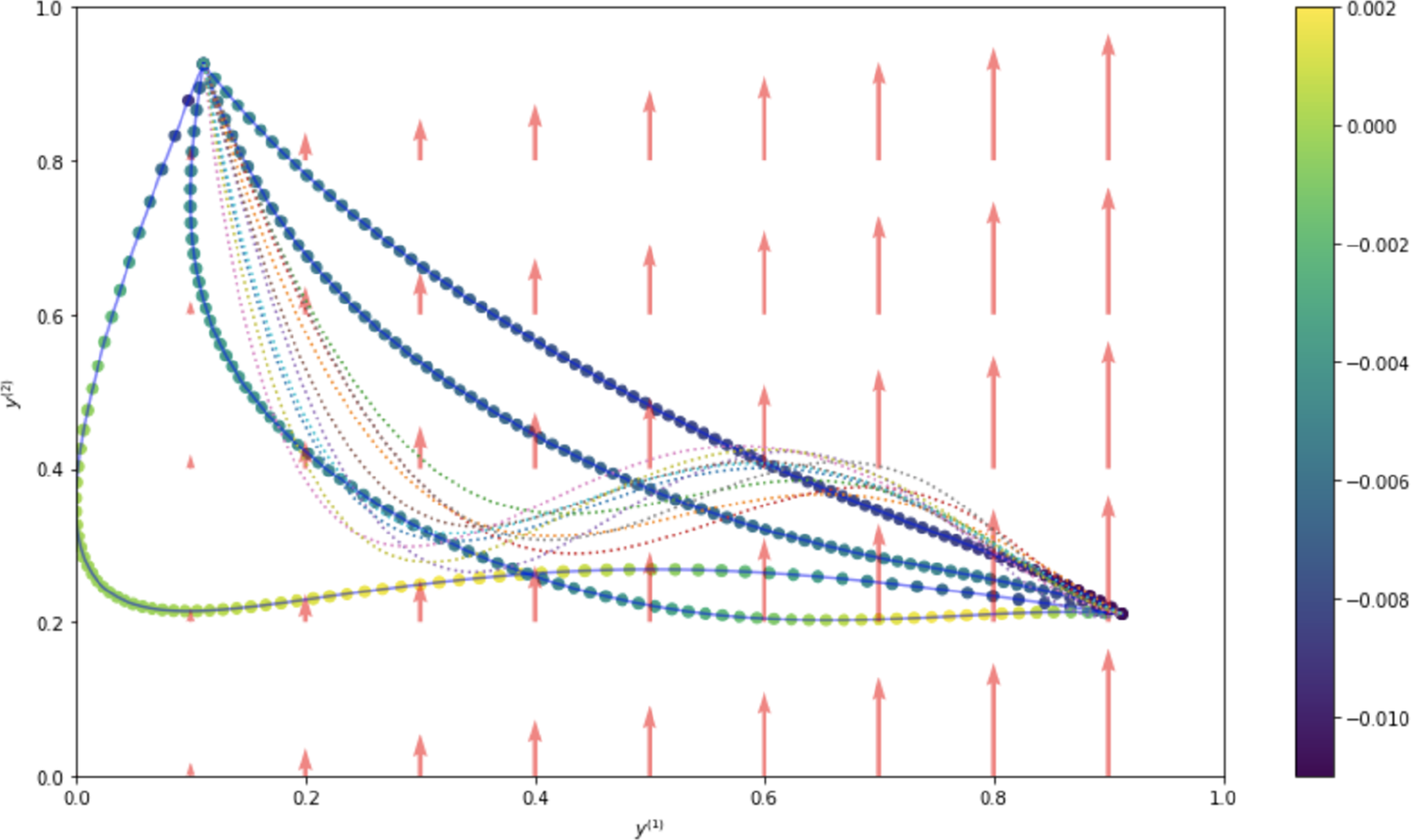
A quantitative comparison in terms of work gains for different values of $ \alpha $
is provided in Table 2. The results confirm the above observations on the curves and show that a right value for
$ \alpha $
is provided in Table 2. The results confirm the above observations on the curves and show that a right value for $ \alpha $
has to be fixed depending on the setting.
$ \alpha $
has to be fixed depending on the setting.
Statistical description of the work gains in percentage for $ \alpha \in \left\{\mathrm{0,0.35,1,10}\right\} $
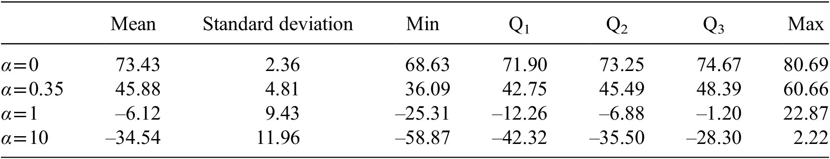
The values have been computed using the 122 available reference trajectories. Negative percentages indicate that no work gains have been obtained. $ {Q}_1 $
,
$ {Q}_1 $
, $ {Q}_2 $
, and
$ {Q}_2 $
, and $ {Q}_3 $
refer to the first, second, and third quartiles.
$ {Q}_3 $
refer to the first, second, and third quartiles.
6. Perspectives
We have proposed an approach for data-driven optimized trajectories without involving dynamical system or numerous constraints. The approach can work based on a known cost function or a cost function learnt from the data. The modeling of the trajectories allows to take into account explicit and implicit linear constraints on the coefficients in the optimization problem. Contrary to full optimization approaches, our method finds a trade-off between high density constraints-compliant solutions and fully optimized solutions through the tuning of the regularization. In the aeronautic framework, our approach leads to promising fuel-efficient trajectories which can be considered by aeronautics experts. Our approach is generic enough to be applied to other physical settings such as the motion of a moving point in a force field (such as a sailing boat).
Some perspectives of this work are first to further exploit the flexibility of Bayesian setting, by not only searching for the mode of the posterior distribution but also sampling by means of MCMC algorithms. A second perspective would be to consider a clustering of reference trajectories, and apply our strategy on each cluster, then particularize the optimal trajectory depending on the cluster. Last but not least, we aim at adapting our approach where some component of the trajectory would be categorical variables: this would be particularly useful for decision making processes in various disciplines.
Acknowledgments
The authors are grateful to Baptiste Gregorutti and Pierre Jouniaux for fruitful discussions about the modeling of the problem and the validation of the results for the aeronautic application.
Data Availability Statement
Data that support the findings of this study have been gathered from the Quick Access Recorder (QAR) of aircrafts operated by a private airline, hence can not be released publicly for commercial reasons.
Author Contributions
Formal analysis: F.D., B.G., and V.V.; Methodology: F.D., B.G., A.T., and V.V.; Software: F.D., A.T.; Writing – original draft: F.D.; Writing – review & editing: B.G., A.T., and V.V. All authors approved the final submitted draft.
Funding Statement
This project has received funding from the Clean Sky 2 Joint Undertaking under the European Union’s Horizon 2020 research and innovation programme under grant agreement No 815914 (PERF-AI). The funder had no role in study design, data collection and analysis, decision to publish, or preparation of the manuscript.
Competing Interests
The authors declare no competing interests exist.
A. Quadratic Cost Computations
Here, we focus on the case where the cost function $ F:\mathcal{C}\left(\left[0,T\right],{\unicode{x211D}}^D\right)\to {\unicode{x211D}}^D $
is of the following form
$ F:\mathcal{C}\left(\left[0,T\right],{\unicode{x211D}}^D\right)\to {\unicode{x211D}}^D $
is of the following form
 $$ F(y)={\int}_0^Ty{(t)}^TQ\hskip0.1em y(t)+{w}^Ty(t)+r\hskip0.1em dt, $$
where $ Q\in {\unicode{x211D}}^{D\times D} $
is symmetric,
$ Q\in {\unicode{x211D}}^{D\times D} $
is symmetric, $ w\in {\unicode{x211D}}^D $
and
$ w\in {\unicode{x211D}}^D $
and $ r\in \unicode{x211D} $
. In this setting, we provide explicit formulas for the costs
$ r\in \unicode{x211D} $
. In this setting, we provide explicit formulas for the costs $ \overset{\check{}}{F}:{\unicode{x211D}}^K\to \unicode{x211D} $
and
$ \overset{\check{}}{F}:{\unicode{x211D}}^K\to \unicode{x211D} $
and $ \tilde{F}:{\unicode{x211D}}^{\sigma}\to \unicode{x211D} $
defined in Section 2.4. A sufficient condition on the parameter
$ \tilde{F}:{\unicode{x211D}}^{\sigma}\to \unicode{x211D} $
defined in Section 2.4. A sufficient condition on the parameter $ \kappa >0 $
so that the optimization problem
$ \kappa >0 $
so that the optimization problem
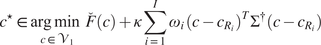 $$ {c}^{\star}\in \underset{c\in {\mathcal{V}}_1}{\arg \hskip0.1em \min \hskip0.3em }\;\overset{\check{}}{F}(c)+\kappa \sum \limits_{i=1}^I{\omega}_i\hskip0.1em {\left(c-{c}_{R_i}\right)}^T{\Sigma}^{\dagger}\left(c-{c}_{R_i}\right) $$
is a quadratic program in the present setting is then derived. From Section 2.4, we recall that the preceding optimization problem is equivalent to
 $$ \left\{\begin{array}{l}{\tilde{c}}_1^{\star}\in \underset{{\tilde{c}}_1\in {\unicode{x211D}}^{\sigma }}{\arg \hskip0.1em \min \hskip0.3em }\tilde{F}\left({\tilde{c}}_1\right)+\kappa \sum \limits_{i=1}^I{\omega}_i\hskip0.1em {\left({\tilde{c}}_1-{\tilde{c}}_{R_i,1}\right)}^T{\Lambda}_{\Sigma, 1}^{-1}\left({\tilde{c}}_1-{\tilde{c}}_{R_i,1}\right),\\ {}{\tilde{c}}_2={V}_2^T{c}_{R_i},\\ {}{\tilde{c}}_3={S}_{A,2}^{-1}\hskip0.1em {U}^T\Gamma .\end{array}\right. $$
Lemma 1.
Suppose that the cost function $ F $
is of the form (20). Then the costs
$ F $
is of the form (20). Then the costs $ \overset{\check{}}{F} $
and
$ \overset{\check{}}{F} $
and $ \tilde{F} $
are quadratic and explicit formulas are given in (24) and (26).
$ \tilde{F} $
are quadratic and explicit formulas are given in (24) and (26).
Proof. Let $ c\in {\unicode{x211D}}^K $
and let
$ c\in {\unicode{x211D}}^K $
and let $ {\left.y:= \Phi \right|}_{{\mathcal{Y}}_{\mathcal{K}}}^{-1}c\in {\mathcal{Y}}_{\mathcal{K}} $
be its associated trajectory, which can be represented as follows:
$ {\left.y:= \Phi \right|}_{{\mathcal{Y}}_{\mathcal{K}}}^{-1}c\in {\mathcal{Y}}_{\mathcal{K}} $
be its associated trajectory, which can be represented as follows:
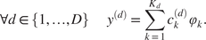 $$ \forall d\in \left\{1,\dots, D\right\}\hskip2em {y}^{(d)}=\sum \limits_{k=1}^{K_d}{c}_k^{(d)}\hskip0.1em {\varphi}_k. $$
We also remark that each component of the vector
 $$ c={\left({c}_1^{(1)},\dots, {c}_{K_1}^{(1)},{c}_1^{(2)},\dots, {c}_{K_2}^{(2)},\dots, {c}_1^{(D)},\dots, {c}_{K_D}^{(D)}\right)}^T $$
can be simply described by a single parameter so that we can write $ c={\left({c}_1,{c}_2,\dots, {c}_K\right)}^T $
.
$ c={\left({c}_1,{c}_2,\dots, {c}_K\right)}^T $
.
-
• Computation of
$ \overset{\check{}}{F} $
:

We first insert the preceding representation of $ y $
into the above quadratic integrand to obtain:
$ y $
into the above quadratic integrand to obtain:
 $$ {\displaystyle \begin{array}{l}y{(t)}^TQ\hskip0.1em y(t)+{w}^Ty(t)+r\\ {}\hskip1.48em =\sum \limits_{d_1,{d}_2=1}^D\sum \limits_{k_1=0}^{K_{d_1}}\sum \limits_{k_2=0}^{K_{d_2}}{Q}_{d_1{d}_2}\hskip0.1em {c}_{k_1}^{\left({d}_1\right)}{c}_{k_2}^{\left({d}_2\right)}\hskip0.1em {\varphi}_{k_1}(t){\varphi}_{k_2}(t)+\sum \limits_{d=1}^D\sum \limits_{k=0}^{K_d}{w}_d\hskip0.1em {c}_k^{(d)}\hskip0.1em {\varphi}_k(t)+r,\end{array}} $$
for all $ t\in \left[0,T\right] $
. The next step of the proof consists in changing the indices of the above sums. To do so, let us define the matrix
$ t\in \left[0,T\right] $
. The next step of the proof consists in changing the indices of the above sums. To do so, let us define the matrix $ \overline{Q}\in {\unicode{x211D}}^{K\times K} $
and the vector
$ \overline{Q}\in {\unicode{x211D}}^{K\times K} $
and the vector $ \overline{w}\in {\unicode{x211D}}^K $
as
$ \overline{w}\in {\unicode{x211D}}^K $
as
 $$ \overline{Q}:= \left(\begin{array}{ccc}{Q}_{11}\hskip0.1em {J}_{K_1,{K}_1}& \dots & {Q}_{1D}\hskip0.1em {J}_{K_1,{K}_D}\\ {}\vdots & & \vdots \\ {}{Q}_{D1}\hskip0.1em {J}_{K_D,{K}_1}& \dots & {Q}_{DD}\hskip0.1em {J}_{K_D,{K}_D}\end{array}\right),\hskip1em \overline{w}:= {\left({w}_1\hskip0.1em {J}_{1,{K}_1}\hskip1em \dots \hskip1em {w}_D\hskip0.1em {J}_{1,{K}_D}\right)}^T, $$
where $ {J}_{m,n} $
is the all-ones matrix of size
$ {J}_{m,n} $
is the all-ones matrix of size $ m\times n $
. We also introduce the map
$ m\times n $
. We also introduce the map $ \overline{\varphi}\in \mathcal{C}\left(\left[0,T\right],{\unicode{x211D}}^K\right) $
as
$ \overline{\varphi}\in \mathcal{C}\left(\left[0,T\right],{\unicode{x211D}}^K\right) $
as
 $$ \overline{\varphi}(t):= {\left({\varphi}_1(t),\dots, {\varphi}_{K_1}(t),{\varphi}_1(t),\dots, {\varphi}_{K_2}(t),\dots, {\varphi}_1(t),\dots, {\varphi}_{K_D}(t)\right)}^T, $$
for all $ t\in \left[0,T\right] $
, where the
$ t\in \left[0,T\right] $
, where the $ {\varphi}_k $
are the functional basis elements. We are now in position to change the indices in the sums appearing in (23):
$ {\varphi}_k $
are the functional basis elements. We are now in position to change the indices in the sums appearing in (23):
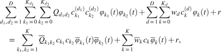 $$ {\displaystyle \begin{array}{l}\sum \limits_{d_1,{d}_2=1}^D\;\sum \limits_{k_1=0}^{K_{d_1}}\;\sum \limits_{k_2=0}^{K_{d_2}}{Q}_{d_1{d}_2}\hskip0.1em {c}_{k_1}^{\left({d}_1\right)}{c}_{k_2}^{\left({d}_2\right)}\hskip0.1em {\varphi}_{k_1}(t){\varphi}_{k_2}(t)+\sum \limits_{d=1}^D\sum \limits_{k=0}^{K_d}{w}_d\hskip0.1em {c}_k^{(d)}\hskip0.1em {\varphi}_k(t)+r\\ {}\hskip1.6em =\sum \limits_{k_1,{k}_2=1}^K{\overline{Q}}_{k_1{k}_2}\hskip0.1em {c}_{k_1}{c}_{k_2}\hskip0.1em {\overline{\varphi}}_{k_1}(t){\overline{\varphi}}_{k_2}(t)+\sum \limits_{k=1}^K{\overline{w}}_k\hskip0.1em {c}_k\hskip0.1em {\overline{\varphi}}_k(t)+r,\end{array}} $$
where we have used the above rewriting of the vector $ c $
. Integrating finally over
$ c $
. Integrating finally over $ \left[0,T\right] $
gives
$ \left[0,T\right] $
gives
 $$ {\displaystyle \begin{array}{c}\overset{\check{}}{F}(c)={\int}_0^Ty{(t)}^TQ\hskip0.1em y(t)+{w}^Ty(t)+r\hskip0.1em dt\\ {}=\sum \limits_{k_1,{k}_2=1}^K{\overline{Q}}_{k_1{k}_2}{\int}_0^T{\overline{\varphi}}_{k_1}(t)\hskip0.1em {\overline{\varphi}}_{k_2}(t)\hskip0.1em dt\hskip0.1em {c}_{k_1}{c}_{k_2}+\sum \limits_{k=1}^K{\overline{w}}_k{\int}_0^T{\overline{\varphi}}_k(t)\hskip0.1em dt\hskip0.1em {c}_k+ rT\\ {}=\sum \limits_{k_1,{k}_2=1}^K{\overset{\check{}}{Q}}_{k_1{k}_2}\hskip0.1em {c}_{k_1}{c}_{k_2}+\sum \limits_{k=1}^K{\overset{\check{}}{w}}_k\hskip0.1em {c}_k+ rT\\ {}={c}^T\overset{\check{}}{Q}c+{\overset{\check{}}{w}}^Tc+ rT,\end{array}} $$
where we have defined
 $$ {\overset{\check{}}{Q}}_{k_1{k}_2}:= {\overline{Q}}_{k_1{k}_2}{\int}_0^T{\overline{\varphi}}_{k_1}(t)\hskip0.1em {\overline{\varphi}}_{k_2}(t)\hskip0.1em dt\hskip2em ,\hskip2em {\overset{\check{}}{w}}_k:= {\overline{w}}_k{\int}_0^T{\overline{\varphi}}_k(t)\hskip0.1em dt. $$
-
• Computation of
$ \tilde{F} $
:

By the definition of $ \tilde{F} $
given in Section 2.4, we have
$ \tilde{F} $
given in Section 2.4, we have
 $$ \tilde{F}\left({\tilde{c}}_1\right)=\overset{\check{}}{F}\left(V{\left({\tilde{c}}_1^T\hskip1em {\tilde{c}}_{2,3}^T\right)}^T\right), $$
where $ V $
has been introduced in Section 2.3 and
$ V $
has been introduced in Section 2.3 and $ {\tilde{c}}_{2,3}\in {\unicode{x211D}}^{K-\sigma } $
is defined as follows:
$ {\tilde{c}}_{2,3}\in {\unicode{x211D}}^{K-\sigma } $
is defined as follows:
 $$ {\tilde{c}}_{2,3}:= \left(\begin{array}{c}{V}_2^T{c}_{R_i}\\ {}{S}_{A,2}^{-1}{U}^T\Gamma \end{array}\right), $$
here the index $ i $
is arbitrarily chosen in
$ i $
is arbitrarily chosen in $ \left\{1,\dots, I\right\} $
since the vector
$ \left\{1,\dots, I\right\} $
since the vector $ {V}_2^T{c}_{R_i} $
has been proved to be independent from
$ {V}_2^T{c}_{R_i} $
has been proved to be independent from $ i $
. We introduce now the matrix
$ i $
. We introduce now the matrix $ {\overset{\check{}}{Q}}_V:= {V}^T\overset{\check{}}{Q}V $
and the vector
$ {\overset{\check{}}{Q}}_V:= {V}^T\overset{\check{}}{Q}V $
and the vector $ {\overset{\check{}}{w}}_V:= {V}^T\overset{\check{}}{w} $
which can be decomposed as follows:
$ {\overset{\check{}}{w}}_V:= {V}^T\overset{\check{}}{w} $
which can be decomposed as follows:
 $$ {\overset{\check{}}{Q}}_V=\left(\begin{array}{cc}{\overset{\check{}}{Q}}_{V,11}& {\overset{\check{}}{Q}}_{V,12}\\ {}{\overset{\check{}}{Q}}_{V,21}& {\overset{\check{}}{Q}}_{V,22}\end{array}\right)\hskip1em ,\hskip1em {\overset{\check{}}{w}}_V=\left(\begin{array}{c}{\overset{\check{}}{w}}_{V,1}\\ {}{\overset{\check{}}{w}}_{V,2}\end{array}\right), $$
where $ {\overset{\check{}}{Q}}_{V,11}\in {\unicode{x211D}}^{\sigma \times \sigma } $
,
$ {\overset{\check{}}{Q}}_{V,11}\in {\unicode{x211D}}^{\sigma \times \sigma } $
, $ {\overset{\check{}}{Q}}_{V,12}\in {\unicode{x211D}}^{\sigma \times \left(K-\sigma \right)} $
,
$ {\overset{\check{}}{Q}}_{V,12}\in {\unicode{x211D}}^{\sigma \times \left(K-\sigma \right)} $
, $ {\overset{\check{}}{Q}}_{V,21}\in {\unicode{x211D}}^{\left(K-\sigma \right)\times \sigma } $
,
$ {\overset{\check{}}{Q}}_{V,21}\in {\unicode{x211D}}^{\left(K-\sigma \right)\times \sigma } $
, $ {\overset{\check{}}{Q}}_{V,22}\in {\unicode{x211D}}^{\left(K-\sigma \right)\times \left(K-\sigma \right)} $
,
$ {\overset{\check{}}{Q}}_{V,22}\in {\unicode{x211D}}^{\left(K-\sigma \right)\times \left(K-\sigma \right)} $
, $ {\overset{\check{}}{w}}_{V,1}\in {\unicode{x211D}}^{\sigma } $
, and
$ {\overset{\check{}}{w}}_{V,1}\in {\unicode{x211D}}^{\sigma } $
, and $ {\overset{\check{}}{w}}_{V,2}\in {\unicode{x211D}}^{K-\sigma } $
. Given this and the preceding point, we obtain
$ {\overset{\check{}}{w}}_{V,2}\in {\unicode{x211D}}^{K-\sigma } $
. Given this and the preceding point, we obtain
 $$ {\displaystyle \begin{array}{c}\tilde{F}\left({\tilde{c}}_1\right)=\left({\tilde{c}}_1^T\hskip1em {\tilde{c}}_{2,3}^T\right)\left({V}^T\overset{\check{}}{Q}V\right){\left({\tilde{c}}_1^T\hskip1em {\tilde{c}}_{2,3}^T\right)}^T+{\left({V}^T\overset{\check{}}{w}\right)}^T{\left({\tilde{c}}_1^T\hskip1em {\tilde{c}}_{2,3}^T\right)}^T+ rT\\ {}=\left({\tilde{c}}_1^T\hskip1em {\tilde{c}}_{2,3}^T\right){\overset{\check{}}{Q}}_V{\left({\tilde{c}}_1^T\hskip1em {\tilde{c}}_{2,3}^T\right)}^T+{\overset{\check{}}{w}}_V^T{\left({\tilde{c}}_1^T\hskip1em {\tilde{c}}_{2,3}^T\right)}^T+ rT\\ {}={\tilde{c}}_1^T\hskip0.1em {\overset{\check{}}{Q}}_{V,11}\hskip0.1em {\tilde{c}}_1+{\tilde{c}}_1^T\hskip0.1em {\overset{\check{}}{Q}}_{V,12}\hskip0.1em {\tilde{c}}_{2,3}+{\tilde{c}}_{2,3}^T\hskip0.1em {\overset{\check{}}{Q}}_{V,21}\hskip0.1em {\tilde{c}}_1+{\tilde{c}}_{2,3}^T\hskip0.1em {\overset{\check{}}{Q}}_{V,22}\hskip0.1em {\tilde{c}}_{2,3}\\ {}\hskip1.48em +{\overset{\check{}}{w}}_{V,1}^T\hskip0.1em {\tilde{c}}_1+{\overset{\check{}}{w}}_{V,2}^T\hskip0.1em {\tilde{c}}_{2,3}+ rT.\end{array}} $$
Rearranging the preceding terms and using the fact that $ {\overset{\check{}}{Q}}_V $
is symmetric gives
$ {\overset{\check{}}{Q}}_V $
is symmetric gives
 $$ \tilde{F}\left({\tilde{c}}_1\right)={\tilde{c}}_1^T\hskip0.1em \tilde{Q}\hskip0.1em {\tilde{c}}_1+{\tilde{w}}^T{\tilde{c}}_1+\tilde{r}, $$
where
 $$ \hskip-15em \bullet \hskip1em \tilde{Q}:= {\overset{\check{}}{Q}}_{V,11}; $$
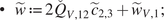 $$ \hskip-7em \bullet \hskip1em \tilde{w}:= 2\hskip0.1em {\overset{\check{}}{Q}}_{V,12}\hskip0.1em {\tilde{c}}_{2,3}+{\tilde{w}}_{V,1}; $$
 $$ \bullet \hskip1em \tilde{r}:= {\tilde{c}}_{2,3}^T\hskip0.1em {\overset{\check{}}{Q}}_{V,22}\hskip0.1em {\tilde{c}}_{2,3}+{\tilde{w}}_{V,2}^T\hskip0.1em {\tilde{c}}_{2,3}+ rT. $$
The optimization problem (22) is then equivalent to the following one in the present quadratic setting:
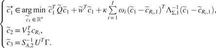 $$ \left\{\begin{array}{l}{\tilde{c}}_1^{\star}\in \underset{{\tilde{c}}_1\in {\unicode{x211D}}^{\sigma }}{\arg \hskip0.1em \min \hskip0.3em }\;{\tilde{c}}_1^T\hskip0.1em \tilde{Q}\hskip0.1em {\tilde{c}}_1+{\tilde{w}}^T{\tilde{c}}_1+\kappa \sum \limits_{i=1}^I{\omega}_i\hskip0.1em {\left({\tilde{c}}_1-{\tilde{c}}_{R_i,1}\right)}^T{\Lambda}_{\Sigma, 1}^{-1}\left({\tilde{c}}_1-{\tilde{c}}_{R_i,1}\right),\\ {}{\tilde{c}}_2={V}_2^T{c}_{R_i},\\ {}{\tilde{c}}_3={S}_{A,2}^{-1}\hskip0.1em {U}^T\Gamma .\end{array}\right. $$
In the following result, we provide a sufficient condition on the parameter $ \kappa >0 $
so that the problem (30) is a quadratic program. The proof uses the fact that the symmetric matrix associated with the quadratic objective function is now explicit and given by the sum of two matrices. A perturbation result for matrices is then applied to obtain a bound for
$ \kappa >0 $
so that the problem (30) is a quadratic program. The proof uses the fact that the symmetric matrix associated with the quadratic objective function is now explicit and given by the sum of two matrices. A perturbation result for matrices is then applied to obtain a bound for $ \kappa $
assuring that the symmetric matrix is positive semidefinite.
$ \kappa $
assuring that the symmetric matrix is positive semidefinite.
Theorem 1.
Let $ {\rho}_1\geqslant {\rho}_2\geqslant \cdots \geqslant {\rho}_{\sigma } $
and
$ {\rho}_1\geqslant {\rho}_2\geqslant \cdots \geqslant {\rho}_{\sigma } $
and $ {\lambda}_1\geqslant {\lambda}_2\geqslant \cdots \geqslant {\lambda}_K $
be respectively the eigenvalues of the symmetric matrices
$ {\lambda}_1\geqslant {\lambda}_2\geqslant \cdots \geqslant {\lambda}_K $
be respectively the eigenvalues of the symmetric matrices $ \tilde{Q} $
and
$ \tilde{Q} $
and $ \Sigma $
. If
$ \Sigma $
. If $ \kappa \geqslant -{\rho}_{\sigma}\hskip0.1em {\lambda}_1 $
then the optimization problem (30) is a quadratic program.
$ \kappa \geqslant -{\rho}_{\sigma}\hskip0.1em {\lambda}_1 $
then the optimization problem (30) is a quadratic program.
Proof. We first note that all the eigenvalues of the matrix $ \Sigma $
are non-negative (because
$ \Sigma $
are non-negative (because $ \Sigma $
is a covariance matrix) and that
$ \Sigma $
is a covariance matrix) and that $ {\lambda}_{\sigma +1}=\dots ={\lambda}_K=0 $
(because
$ {\lambda}_{\sigma +1}=\dots ={\lambda}_K=0 $
(because $ \operatorname{rank}\hskip0.3em \Sigma =\sigma $
). In particular, the eigenvalue
$ \operatorname{rank}\hskip0.3em \Sigma =\sigma $
). In particular, the eigenvalue $ {\lambda}_1 $
is positive.
$ {\lambda}_1 $
is positive.
Standard calculations show that the symmetric matrix associated with the quadratic objective function of the problem (30) is given by
 $$ M\left(\kappa \right):= \tilde{Q}+\kappa \hskip0.1em {\Lambda}_{\Sigma, 1}^{-1}\in {\unicode{x211D}}^{\sigma \times \sigma }. $$
Let $ {\mu}_1\left(\kappa \right)\geqslant {\mu}_2\left(\kappa \right)\geqslant \dots \geqslant {\mu}_{\sigma}\left(\kappa \right) $
denote the eigenvalues of
$ {\mu}_1\left(\kappa \right)\geqslant {\mu}_2\left(\kappa \right)\geqslant \dots \geqslant {\mu}_{\sigma}\left(\kappa \right) $
denote the eigenvalues of $ M\left(\kappa \right) $
. The goal is then to find a sufficient condition on
$ M\left(\kappa \right) $
. The goal is then to find a sufficient condition on $ \kappa >0 $
so that
$ \kappa >0 $
so that $ {\mu}_{\sigma}\left(\kappa \right) $
is non-negative to assure that
$ {\mu}_{\sigma}\left(\kappa \right) $
is non-negative to assure that $ M $
is positive semidefinite. Since
$ M $
is positive semidefinite. Since $ M\left(\kappa \right) $
can be interpreted as a perturbed version of
$ M\left(\kappa \right) $
can be interpreted as a perturbed version of $ \tilde{Q} $
, we can apply Weyl’s inequality (see for instance Wang and Zheng, Reference Wang and Zheng2019) which states
$ \tilde{Q} $
, we can apply Weyl’s inequality (see for instance Wang and Zheng, Reference Wang and Zheng2019) which states
 $$ {\mu}_{\sigma}\left(\kappa \right)\geqslant {\rho}_{\sigma }+\frac{\kappa }{\lambda_1}. $$
Then choosing $ \kappa $
such that
$ \kappa $
such that $ \kappa \geqslant -{\rho}_{\sigma}\hskip0.1em {\lambda}_1 $
implies that
$ \kappa \geqslant -{\rho}_{\sigma}\hskip0.1em {\lambda}_1 $
implies that $ {\mu}_{\sigma}\left(\kappa \right)\geqslant 0 $
, leading to the result.
$ {\mu}_{\sigma}\left(\kappa \right)\geqslant 0 $
, leading to the result.
For the sake of completeness, we finish by rewriting the problem (30) as a quadratic optimization problem in $ {\mathcal{V}}_1\subset {\unicode{x211D}}^K $
.
$ {\mathcal{V}}_1\subset {\unicode{x211D}}^K $
.
Proposition 6.
Suppose that the cost function $ F $
is of the form (20). Then the optimization problem (21) is equivalent to the following one:
$ F $
is of the form (20). Then the optimization problem (21) is equivalent to the following one:
 $$ {c}^{\star}\in \underset{c\in {\mathcal{V}}_1}{\arg \hskip0.1em \min}\;{c}^T\left(\overset{\check{}}{Q}+\kappa \hskip0.1em {\Sigma}^{\dagger}\right)c+{\left(\overset{\check{}}{w}-2\kappa \sum \limits_{i=1}^I{\omega}_i\hskip0.1em {\Sigma}^{\dagger }{c}_{R_i}\right)}^Tc. $$
Proof. It is sufficient to show that the two following objective functions $ {g}_1,{g}_2:{\unicode{x211D}}^K\to \unicode{x211D} $
have the same minima:
$ {g}_1,{g}_2:{\unicode{x211D}}^K\to \unicode{x211D} $
have the same minima:
-
•
$ {g}_1(c):= \overset{\check{}}{F}(c)+\kappa \sum_{i=1}^I{\omega}_i\hskip0.1em {\left(c-{c}_{R_i}\right)}^T{\Sigma}^{\dagger}\left(c-{c}_{R_i}\right) $
; -
•
$ {g}_2(c):= {c}^T\left(\overset{\check{}}{Q}+\kappa \hskip0.1em {\Sigma}^{\dagger}\right)c+{\left(\overset{\check{}}{w}-2\kappa \sum_{i=1}^I{\omega}_i\hskip0.1em {\Sigma}^{\dagger }{c}_{R_i}\right)}^Tc $
.


First, we have by standard calculations,
 $$ {\displaystyle \begin{array}{c}\sum \limits_{i=1}^I{\omega}_i\hskip0.1em {\left(c-{c}_{R_i}\right)}^T{\Sigma}^{\dagger}\left(c-{c}_{R_i}\right)=\sum \limits_{i=1}^I{\omega}_i\hskip0.1em {c}^T{\Sigma}^{\dagger }c-2\sum \limits_{i=1}^I{\omega}_i\hskip0.1em {c}_{R_i}^T{\Sigma}^{\dagger }c+\sum \limits_{i=1}^I{\omega}_i\hskip0.1em {c}_{R_i}^T{\Sigma}^{\dagger }{c}_{R_i}\\ {}={c}^T{\Sigma}^{\dagger }c-{\left(2\sum \limits_{i=1}^I{\omega}_i\hskip0.1em {\Sigma}^{\dagger }{c}_{R_i}\right)}^Tc+\sum \limits_{i=1}^I{\omega}_i\hskip0.1em {c}_{R_i}^T{\Sigma}^{\dagger }{c}_{R_i},\end{array}} $$
for any $ c\in {\unicode{x211D}}^K $
, where we have used
$ c\in {\unicode{x211D}}^K $
, where we have used $ {\sum}_{i=1}^I{\omega}_i=1 $
. Combining now this equality with Lemma 1 implies
$ {\sum}_{i=1}^I{\omega}_i=1 $
. Combining now this equality with Lemma 1 implies
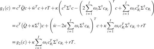 $$ {\displaystyle \begin{array}{c}{g}_1(c)={c}^T\overset{\check{}}{Q}c+{\overset{\check{}}{w}}^Tc+ rT+\kappa \left({c}^T{\Sigma}^{\dagger }c-{\left(2\sum \limits_{i=1}^I{\omega}_i\hskip0.1em {\Sigma}^{\dagger }{c}_{R_i}\right)}^Tc+\sum \limits_{i=1}^I{\omega}_i\hskip0.1em {c}_{R_i}^T{\Sigma}^{\dagger }{c}_{R_i}\right)\\ {}={c}^T\left(\overset{\check{}}{Q}+\kappa \hskip0.1em {\Sigma}^{\dagger}\right)c+{\left(\overset{\check{}}{w}-2\kappa \sum \limits_{i=1}^I{\omega}_i\hskip0.1em {\Sigma}^{\dagger }{c}_{R_i}\right)}^Tc+\kappa \sum \limits_{i=1}^I{\omega}_i\hskip0.1em {c}_{R_i}^T{\Sigma}^{\dagger }{c}_{R_i}+ rT\\ {}={g}_2(c)+\kappa \sum \limits_{i=1}^I{\omega}_i\hskip0.1em {c}_{R_i}^T{\Sigma}^{\dagger }{c}_{R_i}+ rT.\end{array}} $$
Since the two last terms of the last right-hand side do not depend on $ c $
, we deduce that the objective functions
$ c $
, we deduce that the objective functions $ {g}_1 $
and
$ {g}_1 $
and $ {g}_2 $
have the same minima.
$ {g}_2 $
have the same minima.


 Open access
Comments
No Comments have been published for this article.