


Impact statement
Railway-induced vibrations can disturb residents, interfere with sensitive instruments, and damage historical structures near railway corridors. In Europe, over 7.5 million residents are potentially affected by railway noise and vibrations. An effective approach to attenuate vibration levels at receiving points is to minimize the vibration source, which requires an accurate predictive model for assessing tunnel–soil interaction under dynamic loading conditions. While various models exist, none offer rapid and precise predictions suitable for complex tunnel–soil interaction problems and computationally demanding optimization tasks. This study presents an instant prediction model for optimizing the geometry and materials of underground railway tunnels, enabling industries to design tunnels based on specified constraints, with the objective of minimizing the elastic waves propagated into the surrounding soil.
1. Introduction
Dynamic soil–structure interaction (SSI) is an engineering discipline situated at the intersection of soil science and structural dynamics. It is closely related to fields such as earthquake engineering, geophysics, geomechanics, materials science, and computational mechanics (Kausel, Reference Kausel2006). Over recent decades, scientific and technical communities have shown growing interest in the dynamic assessment of SSI problems. Concurrently, a wide variety of modeling methodologies have been developed to address these complex engineering challenges. For SSI problems that can be assumed to be longitudinally invariant, such as railway tracks (Galvín et al., Reference Galvín, François, Schevenels, Bongini, Degrande and Lombaert2010), tunnels (Galvín et al., Reference Galvín, François, Schevenels, Bongini, Degrande and Lombaert2010; Jin et al., Reference Jin, Thompson, Lurcock, Toward and Ntotsios2018), roads (François et al., Reference François, Schevenels, Galvín, Lombaert and Degrande2010), and pipelines (Ozdemir et al., Reference Ozdemir, Coulier, Lak, François, Lombaert and Degrande2013), 2.5D modeling approaches (Lombaert et al., Reference Lombaert, Degrande, François and Thompson2015) have proven to be a more efficient alternative to full 3D models (Andersen and Jones, Reference Andersen and Jones2006). The wavenumber–frequency domain has been widely adopted in models examining dynamic SSI between the soil and various types of infrastructure, including at-grade railway tracks (François et al., Reference François, Schevenels, Galvín, Lombaert and Degrande2010; Galvín et al., Reference Galvín, François, Schevenels, Bongini, Degrande and Lombaert2010), underground tunnel systems (Galvín et al., Reference Galvín, François, Schevenels, Bongini, Degrande and Lombaert2010; Jin et al., Reference Jin, Thompson, Lurcock, Toward and Ntotsios2018), roads (Lombaert et al., Reference Lombaert, Degrande and Clouteau2000), and pipelines (Ozdemir et al., Reference Ozdemir, Coulier, Lak, François, Lombaert and Degrande2013). This paper particularly focuses on underground railway tunnel–soil–structure interaction problems, as shown in Figure 1. It is important to note that the methodology developed in this study takes into account the full-space model of the soil. In the following sections, the existing studies on numerical models for the assessment of underground railway tunnel–soil interaction problems are presented, along with the introduction of surrogate models and optimization algorithms in this context.
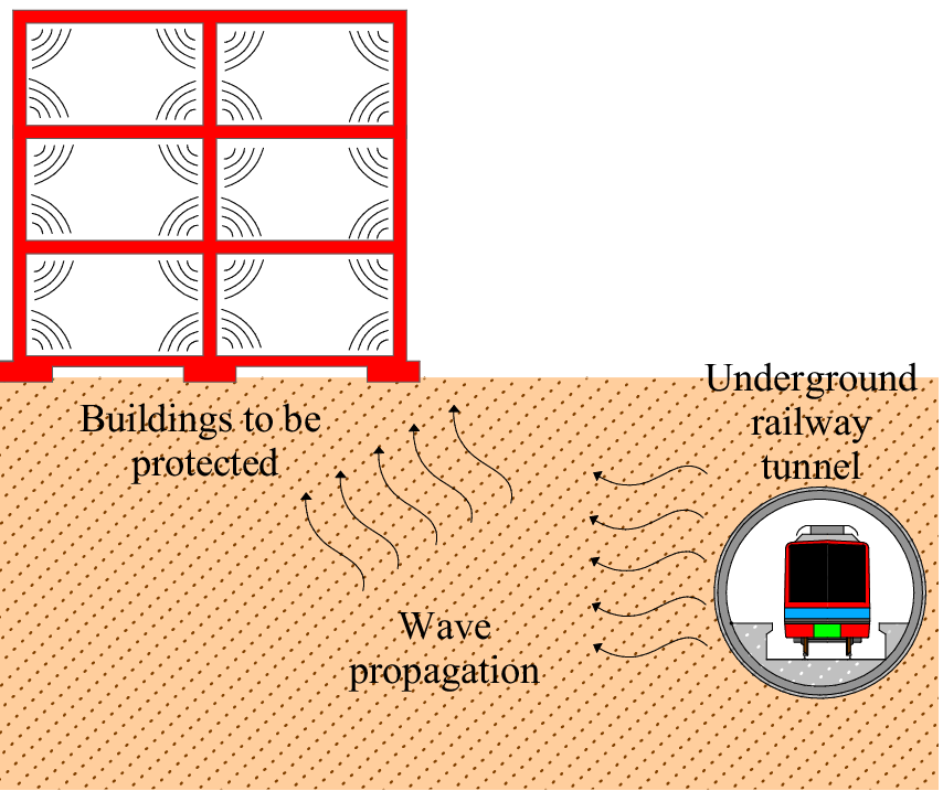
Figure 1. Schematic description of the underground railway tunnel–soil interaction problem.
1.1. 2.5D numerical models for SSI problems in elastodynamics
The applicability of 2.5D modeling approaches to SSI problems was first introduced through an application of 2.5D finite element method (FEM) to soil–structure systems (Hwang and Lysmer, Reference Hwang and Lysmer1981). Subsequently, a 2.5D approach incorporating finite and infinite elements was developed to model longitudinally invariant unbounded systems subjected to moving loads, with infinite elements employed to represent the unbounded domain (Yang and Hung, Reference Yang and Hung2001). A widely adopted method for addressing SSI problems is the coupled FEM–boundary element method (BEM), where FEM is applied to model the structure and BEM is used to represent the soil medium. In this context, a 2.5D FEM–BEM approach was developed (Sheng et al., Reference Sheng, Jones and Thompson2005). Another notable contribution involved the utilization of Green’s functions for a layered half-space as fundamental solutions, instead of full-space ones, resulting in a significant reduction in the number of boundaries requiring meshing (François et al., Reference François, Schevenels, Galvín, Lombaert and Degrande2010). This method has been applied to predict railway-induced vibrations (Galvín et al., Reference Galvín, François, Schevenels, Bongini, Degrande and Lombaert2010). An alternate strategy for deriving Green’s functions needed for 2.5D BEM in elastodynamics is the thin layer method (De Oliveira Barbosa et al., Reference De Oliveira Barbosa, Kausel, Azevedo and Calçada2015). Furthermore, a 2.5D FEM–perfectly matched layer (PML) approach was introduced to study vibrations in buildings caused by underground railway traffic, employing FEM to model the structure and PML to represent the unbounded soil domain (Lopes et al., Reference Lopes, Costa, Ferraz, Calçada and Cardoso2014).
Meshless methods, as an alternative to traditional mesh-based approaches, have garnered increasing interest from the research community over the past decades. These methods do not rely on a predefined mesh topology, leading to simpler formulations and computational implementation procedures, while maintaining the robustness and accuracy of mesh-based approaches (Liravi, Reference Liravi2022). In recent years, numerous studies have focused on the development of novel meshless approaches. Among these, the method of fundamental solutions (MFS) and the singular boundary method (SBM) are particularly well known. For instance, a 2.5D FEM–BEM–MFS approach has been proposed, wherein the BEM is first used to calculate SSI forces, followed by the application of the MFS to compute radiated elastic waves (Liravi et al., Reference Liravi, Arcos, Ghangale, Noori and Romeu2021). Despite the advantages of hybrid approaches such as FEM–MFS (Amado-Mendes et al., Reference Amado-Mendes, Alves Costa, Godinho and Lopes2015; Colaço et al., Reference Colaço, Costa, Amado-Mendes and Calçada2021) and FEM–BEM–MFS, significant challenges remain when dealing with complex boundary shapes, including geometric singularities. To address these challenges, modified meshless strategies have been introduced, such as the FEM–SBM approach (Liravi, Reference Liravi2022). In the most recent developments, a hybrid method combining both the SBM and the MFS, referred to as the hybrid SBM–MFS, has been developed. This method capitalizes on the strengths of both techniques and is particularly effective for addressing problems involving geometric singularities in elastic (Liravi et al., Reference Liravi, Clot, Arcos, Fakhraei, Godinho, Conto and Romeu2024) and acoustic (Fakhraei et al., Reference Fakhraei, Arcos, Pàmies, Liravi, Godinho and Romeu2024) media.
Numerous alternative meshless methods have been proposed in the literature. For instance, the regularized meshless method was first introduced by Young et al. (Reference Young, Chen and Lee2005) and later enhanced by incorporating the double-layer potential into the desingularization procedure (Liu, Reference Liu2017). Another technique, known as the boundary-distributed source approach, replaces concentrated sources with circularly distributed ones, resulting in a singularity-free method (Kim, Reference Kim2013). Additional meshless methods discussed in the literature include the dual surface method (Fakhraei et al., Reference Fakhraei, Arcos, Pàmies, Liravi and Romeu2023), the boundary knot method (Sun et al., Reference Sun, Zhang and Yu2020), the localized boundary knot method (Wang et al., Reference Wang, Gu, Qu and Zhang2020; Yue et al., Reference Yue, Wang, Zhang and Zhang2021), and the local Petrov–Galerkin method (Dehghan and Salehi, Reference Dehghan and Salehi2014). Although meshless methods are competitive in terms of efficiency for dynamic SSI problems, they still incur substantial computational time. Moreover, due to the inherent complexity of these problems, they limit the feasibility of a systematic investigation of design options.
1.2. Surrogate models
To reduce the lead time from design, that is, by varying the simulation parameters, to analysis results, surrogate models can be employed. This technique reconstructs the solution space by appropriate interpolation paradigms. It is successfully applied in several geotechnical problems, such as tunnel track design (Bui et al., Reference Bui, Cao, Freitag, Hackl and Meschke2023), real-time prediction of settlement (Cao et al., Reference Cao, Freitag and Meschke2016), or vibrations induced by pile driving (Abouelmaty et al., Reference Abouelmaty, Colaço, Fares, Ramos and Costa2024). Typical surrogate models include proper orthogonal decomposition using radial basis functions, Artificial Neural Network (ANN)-based models, and gradient boosting approach.
In the Proper Orthogonal Decomposition (POD) approach, snapshots are constructed by extracting information from the numerical results. This is often encoded in the vector form. Principal component analysis, such as Singular Value Decomposition (SVD) decomposition, is then used to extract the eigenvalues and eigenvectors. For the large problem, only several largest eigenvalues are kept to retain the most information of the input data. The interpolated solution of the original problem can then be reconstructed by employing Radial Basis Functions (Freitag et al., Reference Freitag, Cao, Ninić and Meschke2015; Bui et al., Reference Bui, Cao, Freitag, Hackl and Meschke2023).
Instead of performing numerical analysis on the snapshots, ANN approach mimics the way the human brain facilitates information by embedding the prediction data in the network weights via progressive training (Ninić and Meschke, Reference Ninić and Meschke2015; Ninic et al., Reference Ninic, Alsahly, Vonthron, Bui, Koch, König and Meschke2021). For numerical prediction tasks, a feedforward network is usually sufficient. Nevertheless, convolutional neural networks show to be exceptional in prediction involving temporal and historical data. However, in Bui et al. (Reference Bui, Cao, Freitag, Hackl and Meschke2023), ANN is shown not to be as accurate as the POD approach for the numerical prediction task for the same computational effort.
Hybrid approaches are also developed to improve the efficiency and reliability of surrogate models. For example, Freitag et al. (Reference Freitag, Cao, Ninić and Meschke2015) and Cao et al. (Reference Cao, Freitag and Meschke2016) combine POD and ANN for application in mechanized tunneling. Another branch of machine learning, the so-called Ensemble learning, has also gained widespread use in the geotechnical community (Thai et al., Reference Thai, Tu, Bui and Bui2021; Xu et al., Reference Xu, Cao, Yuan and Meschke2023). This technique relies on simpler learning models and uses boosting methods to connect and improve the robustness of the integral model.
1.3. Optimization algorithms
The surrogate model usually provides sufficiently smoothed output space for the optimization problem. In this regard, local optimization can be used, providing that the second gradient of the output with respect to the input space exists. In this case, the steepest descent approach or Newton Raphson algorithm will provide a quadratic converged solution efficiently. Nevertheless, for real applications, when the input parameters vary greatly and have intricate coupling, the local optimization may resort to a local minima solution (Nocedal and Wright, Reference Nocedal and Wright2006). This effect becomes more profound if there are additional constraints. As a result, a locally optimized solution may not be the global one. To overcome this, a global optimization algorithm is required (Liravi et al., Reference Liravi, Fakhraei, Kaewunruen, Fu and Ninić2025). This method of searching for an optimized solution typically employs an evolutionary approach where an initial solution is created. The solution is then improved gradually by searching in the appropriate domains. To avoid the local minima, an exhaustive search can be used or a disruptive solution can be fabricated as in the case of genetic algorithms (Petrowski and Ben-Hamida, Reference Petrowski and Ben-Hamida2017). In particle swarm optimization, multiple solutions are defined in the swarm of particles, which then be steered toward the global optimum by simulating the social behavior of moving organisms (Ninić et al., Reference Ninić, Freitag and Meschke2017). This type of optimization method, together with the genetic algorithm, adopts the natural behavior and is heuristic by default.
Despite advancements in global optimization methods, many rely on iterative evaluations of computationally expensive objective functions, limiting their applicability in real-world engineering problems (Moens and Hanss, Reference Moens and Hanss2011). This gap highlights the need for a more efficient approach capable of balancing exploration and exploitation while minimizing computational costs. Bayesian optimization offers a compelling alternative for such scenarios (Shahriari et al., Reference Shahriari, Swersky, Wang, Adams and Freitas2016; Diessner et al., Reference Diessner, Wilson and Whalley2024). By leveraging surrogate models, Bayesian optimization intelligently selects the next evaluation points based on probabilistic estimates of the objective function. This method not only reduces the number of required evaluations but also adapts to high-dimensional, noisy, and constrained problems (Shahriari et al., Reference Shahriari, Swersky, Wang, Adams and Freitas2016), making it particularly well suited for tunnel–soil interaction problems or other scenarios with complex input–output coupling.
1.4. Problem statement and novelty
The optimization of geometrical and material properties in tunnel–soil interaction problems under elastodynamic conditions remains a challenging task due to the high computational cost of conventional meshless or mesh-based approaches. While surrogate models have shown promise in smoothing the output space to enhance optimization performance (Liu et al., Reference Liu, Sun, Zhang, Grout and Gielen2016), their application to minimizing elastic wave propagation in the surrounding soil, by optimizing specific tunnel design parameters, has not been thoroughly investigated. This gap highlights the need for research into integrating surrogate models with optimization algorithms to address this computationally intensive problem effectively (Khowaja et al., Reference Khowaja, Shcherbatyy and Härdle2019).
In this paper, a 2.5D FEM–SBM numerical method is employed to develop a surrogate model for longitudinally invariant SSI problems. In the 2.5D FEM–SBM approach, the structure is modeled using the 2.5D FEM, while a 2.5D SBM approach is adopted to represent the surrounding soil. The novelty of the present study lies in two key aspects. First, the combination of the versatility of the 2.5D FEM with the accuracy of the 2.5D SBM, along with the use of the Latin hypercube sampling (LHS) technique, ensures that the developed regression ensemble model is both accurate and well suited for optimization tasks. This makes it a valuable alternative for the rapid assessment of underground railway tunnel–soil interaction problems in elastodynamics, specifically for cases with invariant longitudinal cross-sections. Second, the optimization algorithm takes into account both material and geometrical aspects of the underground railway tunnel structure. The integration of these two key elements makes this study the first to develop a surrogate for the optimization of underground railway tunnels from both material and geometrical perspectives, with the objective of minimizing the elastic waves propagated from the tunnel into the surrounding soil.
The remainder of this paper is structured as follows: Section 2 introduces the governing equations of the problem and the mathematical formulation of the 2D FEM–SBM approach. Section 3 describes the surrogate model used in this study and presents two examples to validate the developed surrogate model. Section 4 focuses on the optimization of underground railway tunnels with circular and rectangular cross-sections. Section 5 evaluates the performance of the optimized cases across the entire frequency range. Finally, the key findings of this study are summarized in Section 6.
2. Numerical formulation
The general description of the 2.5D FEM–SBM approach, which will be replaced by the surrogate model, is illustrated in Figure 2. The structure is modeled using FEM, while the unbounded domain representing the soil is modeled using SBM. The SBM method approximates the solution for the displacement and traction fields in the soil by employing a set of virtual sources placed along the boundary, which satisfy the boundary conditions evaluated at the collocation points, also distributed along the boundary. Further details of the method can be found in Liravi (Reference Liravi2022).
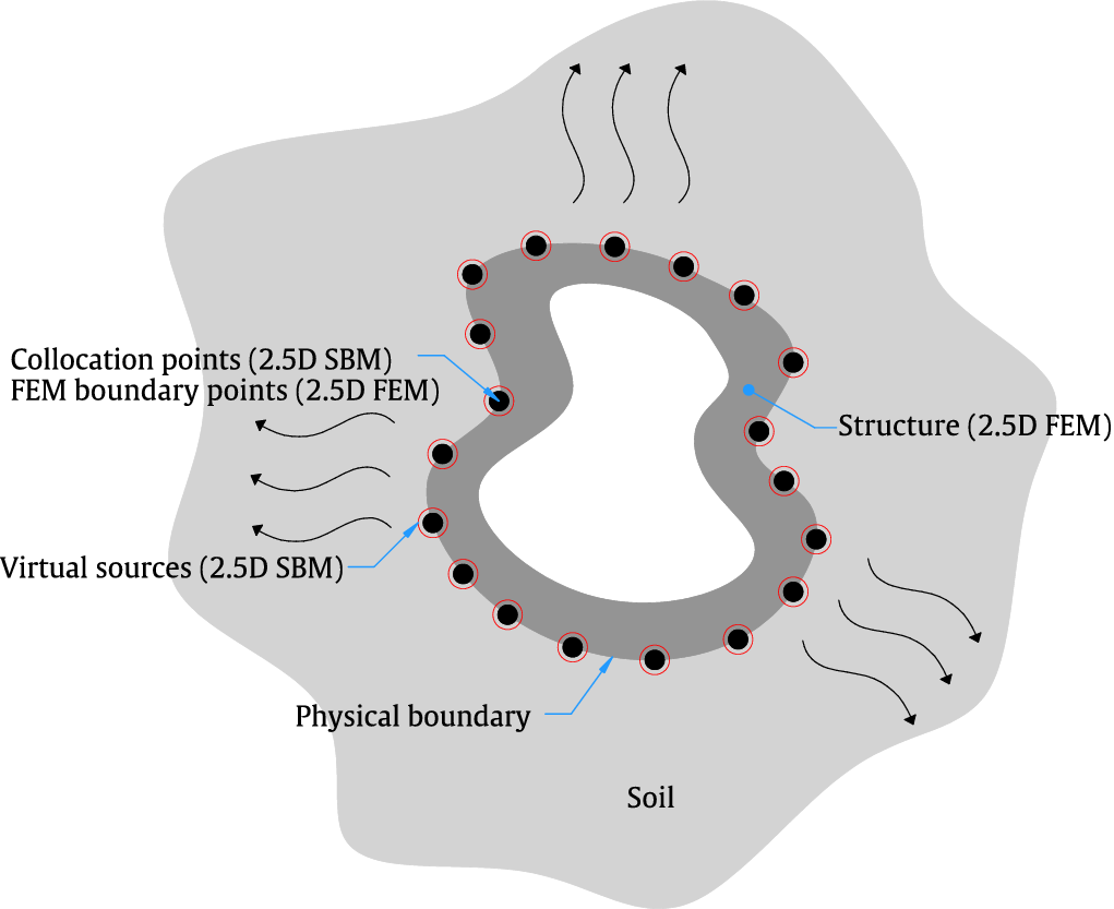
Figure 2. General description of the proposed 2.5D FEM–SBM methodology. Collocation and FEM boundary nodes are represented by black solid points, while virtual forces are indicated by red circles.
2.1. Governing equations
The governing equations of elastodynamics are presented in this section. Consider the motion of a homogeneous, isotropic elastic solid occupying a three-dimensional region $ \Omega $
, enclosed by the boundary
$ \Omega $
, enclosed by the boundary $ \Gamma $
. Assuming the absence of body forces, the governing equation in Cartesian coordinates in the frequency domain for the solid is given by (Kausel, Reference Kausel2006)
$ \Gamma $
. Assuming the absence of body forces, the governing equation in Cartesian coordinates in the frequency domain for the solid is given by (Kausel, Reference Kausel2006)
 $$ \mu {\mathbf{\nabla}}^2\mathbf{U}+\left(\lambda +\mu \right)\mathbf{\nabla}\left(\mathbf{\nabla}\cdot \mathbf{U}\right)+{\rho \omega}^2\mathbf{U}=0,\hskip1em \mathbf{x}\in \Omega, $$
where $ \mathbf{U}={\left[{U}_x,{U}_y,{U}_z\right]}^{\mathrm{T}} $
denotes the displacement vector at a position
$ \mathbf{U}={\left[{U}_x,{U}_y,{U}_z\right]}^{\mathrm{T}} $
denotes the displacement vector at a position $ \mathbf{x}={\left[x,y,z\right]}^{\mathrm{T}} $
,
$ \mathbf{x}={\left[x,y,z\right]}^{\mathrm{T}} $
, $ \mathbf{\nabla}={\left[\frac{\partial }{\partial x},\frac{\partial }{\partial y},\frac{\partial }{\partial z}\right]}^{\mathrm{T}} $
represents the gradient operator, and
$ \mathbf{\nabla}={\left[\frac{\partial }{\partial x},\frac{\partial }{\partial y},\frac{\partial }{\partial z}\right]}^{\mathrm{T}} $
represents the gradient operator, and $ \rho $
is the mass density. The angular frequency is defined as
$ \rho $
is the mass density. The angular frequency is defined as $ \omega =2\pi f $
, where
$ \omega =2\pi f $
, where $ f $
is the frequency in Hertz. The Lamé constants are given by
$ f $
is the frequency in Hertz. The Lamé constants are given by $ \lambda =\frac{\nu E}{\left(1+\nu \right)\left(1-2\nu \right)} $
and
$ \lambda =\frac{\nu E}{\left(1+\nu \right)\left(1-2\nu \right)} $
and $ \mu =\frac{E}{2\left(1+\nu \right)} $
, with
$ \mu =\frac{E}{2\left(1+\nu \right)} $
, with $ E $
being Young’s modulus and
$ E $
being Young’s modulus and $ \nu $
the Poisson ratio.
$ \nu $
the Poisson ratio.
For this boundary value problem, Dirichlet or Neumann boundary conditions are typically imposed as follows:
 $$ \mathbf{U}={\mathbf{U}}_b,\hskip1em \mathbf{x}\in \Gamma, $$
 $$ \mathbf{T}=\boldsymbol{\sigma} \cdot \mathbf{n}={\mathbf{T}}_b,\hskip1em \mathbf{x}\in \Gamma, $$
where $ \mathbf{n}={\left[{n}_x,{n}_y,{n}_z\right]}^{\mathrm{T}} $
represents the outward unit normal vector to the boundary,
$ \mathbf{n}={\left[{n}_x,{n}_y,{n}_z\right]}^{\mathrm{T}} $
represents the outward unit normal vector to the boundary, $ \mathbf{T} $
is the vector containing the three components of the traction field,
$ \mathbf{T} $
is the vector containing the three components of the traction field, $ \boldsymbol{\sigma} $
is the stress tensor, and the prescribed values for the displacement and traction boundary conditions are denoted by the vectors
$ \boldsymbol{\sigma} $
is the stress tensor, and the prescribed values for the displacement and traction boundary conditions are denoted by the vectors $ {\mathbf{U}}_b $
and
$ {\mathbf{U}}_b $
and $ {\mathbf{T}}_b $
, respectively. The components of the stress tensor for an isotropic medium are defined as
$ {\mathbf{T}}_b $
, respectively. The components of the stress tensor for an isotropic medium are defined as
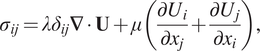 $$ {\sigma}_{ij}={\lambda \delta}_{ij}\mathbf{\nabla}\cdot \mathbf{U}+\mu \left(\frac{\partial {U}_i}{\partial {x}_j}+\frac{\partial {U}_j}{\partial {x}_i}\right), $$
where the indices $ i $
and
$ i $
and $ j $
can take values
$ j $
can take values $ 1 $
,
$ 1 $
, $ 2 $
, or
$ 2 $
, or $ 3 $
, representing the coordinates
$ 3 $
, representing the coordinates $ x $
,
$ x $
, $ y $
, and
$ y $
, and $ z $
, respectively, and where
$ z $
, respectively, and where $ {\delta}_{ij} $
is the Kronecker delta.
$ {\delta}_{ij} $
is the Kronecker delta.
When the system under study satisfies the condition of longitudinal invariance of its mechanical and geometrical parameters, it is often convenient to formulate the problem in the wavenumber–frequency domain, referred to as the 2.5D domain. The method presented in this paper is specifically designed for such problems. Assuming $ x $
as the direction of invariance, the governing equation and boundary conditions are transformed into the wavenumber domain using a Fourier transform of the form:
$ x $
as the direction of invariance, the governing equation and boundary conditions are transformed into the wavenumber domain using a Fourier transform of the form:
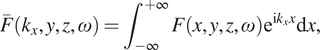 $$ \overline{F}\left({k}_x,y,z,\omega \right)={\int}_{-\infty}^{+\infty}\;F\left(x,y,z,\omega \right){\mathrm{e}}^{\mathrm{i}{k}_xx}\mathrm{d}x, $$
where $ {k}_x $
is the wavenumber associated with the longitudinal direction
$ {k}_x $
is the wavenumber associated with the longitudinal direction $ x $
,
$ x $
, $ F $
represents displacements
$ F $
represents displacements $ U $
or tractions
$ U $
or tractions $ T $
in the spatial–frequency domain, and
$ T $
in the spatial–frequency domain, and $ \overline{F} $
denotes the corresponding quantities in the wavenumber–frequency domain. The detailed derivation is provided in Tadeu et al. (Reference Tadeu, António and Godinho2001). For the sake of brevity, it is not included in the present paper.
$ \overline{F} $
denotes the corresponding quantities in the wavenumber–frequency domain. The detailed derivation is provided in Tadeu et al. (Reference Tadeu, António and Godinho2001). For the sake of brevity, it is not included in the present paper.
2.2. 2.5D FEM–SBM methodology
Using radial basis function interpolation, the displacement and traction of the soil are approximated by the following linear combinations of fundamental solutions corresponding to $ N $
distinct source points:
$ N $
distinct source points:
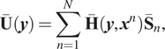 $$ \overline{\mathbf{U}}\left(\boldsymbol{y}\right)=\sum \limits_{n=1}^N\;\overline{\mathbf{H}}\left(\boldsymbol{y},{\boldsymbol{x}}^n\right){\overline{\mathbf{S}}}_n, $$
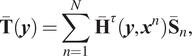 $$ \overline{\mathbf{T}}\left(\boldsymbol{y}\right)=\sum \limits_{n=1}^N\;{\overline{\mathbf{H}}}^{\tau}\left(\boldsymbol{y},{\boldsymbol{x}}^n\right){\overline{\mathbf{S}}}_n, $$
Here, $ \overline{\mathbf{U}}\left(\boldsymbol{y}\right) $
and
$ \overline{\mathbf{U}}\left(\boldsymbol{y}\right) $
and $ \overline{\mathbf{T}}\left(\boldsymbol{y}\right) $
represent the soil displacements and tractions, respectively, at an arbitrary field point
$ \overline{\mathbf{T}}\left(\boldsymbol{y}\right) $
represent the soil displacements and tractions, respectively, at an arbitrary field point $ \boldsymbol{y} $
. The vector
$ \boldsymbol{y} $
. The vector $ {\overline{\mathbf{S}}}_n $
denotes the unknown strengths of the
$ {\overline{\mathbf{S}}}_n $
denotes the unknown strengths of the $ n $
th virtual source located at
$ n $
th virtual source located at $ {\boldsymbol{x}}^n $
, while
$ {\boldsymbol{x}}^n $
, while $ \overline{\mathbf{H}}\left(\boldsymbol{y},{\boldsymbol{x}}^n\right) $
and
$ \overline{\mathbf{H}}\left(\boldsymbol{y},{\boldsymbol{x}}^n\right) $
and $ {\overline{\mathbf{H}}}^{\tau}\left(\boldsymbol{y},{\boldsymbol{x}}^n\right) $
are the soil’s dynamic Green’s functions for displacement and traction, respectively.
$ {\overline{\mathbf{H}}}^{\tau}\left(\boldsymbol{y},{\boldsymbol{x}}^n\right) $
are the soil’s dynamic Green’s functions for displacement and traction, respectively.
The SBM method assumes that these equations can be reformulated as follows (Liravi, Reference Liravi2022):
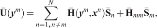 $$ \overline{\mathbf{U}}\left({\boldsymbol{y}}^m\right)=\sum \limits_{n=1,n\ne m}^N\overline{\mathbf{H}}\left({\boldsymbol{y}}^m,{\boldsymbol{x}}^n\right){\overline{\mathbf{S}}}_n+{\overline{\mathbf{H}}}_{mm}{\overline{\mathbf{S}}}_m, $$
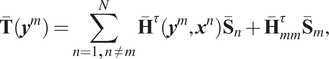 $$ \overline{\mathbf{T}}\left({\boldsymbol{y}}^m\right)=\sum \limits_{n=1,n\ne m}^N{\overline{\mathbf{H}}}^{\tau}\left({\boldsymbol{y}}^m,{\boldsymbol{x}}^n\right){\overline{\mathbf{S}}}_n+{\overline{\mathbf{H}}}_{mm}^{\tau }{\overline{\mathbf{S}}}_m, $$
where $ {\boldsymbol{y}}^m $
refers to the position of the
$ {\boldsymbol{y}}^m $
refers to the position of the $ m $
th collocation point, and
$ m $
th collocation point, and $ {\overline{\mathbf{H}}}_{mm} $ $ {\overline{\mathbf{H}}}_{mm}^{\tau } $
are known as origin intensity factors (OIFs) in the SBM literature. The term “OIF” for the Neumann boundary conditions is defined in Eq. (2.8):
$ {\overline{\mathbf{H}}}_{mm}^{\tau } $
are known as origin intensity factors (OIFs) in the SBM literature. The term “OIF” for the Neumann boundary conditions is defined in Eq. (2.8):
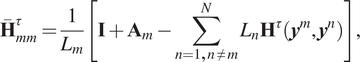 $$ {\overline{\mathbf{H}}}_{mm}^{\tau }=\frac{1}{L_m}\left[\mathbf{I}+{\mathbf{A}}_m-\sum \limits_{n=1,n\ne m}^N{L}_n{\mathbf{H}}^{\tau}\left({\boldsymbol{y}}^m,{\boldsymbol{y}}^n\right)\right], $$
where $ \mathbf{I} $
is the identity matrix and
$ \mathbf{I} $
is the identity matrix and $ {L}_i $
is the half-length of the curve between the source points
$ {L}_i $
is the half-length of the curve between the source points $ {\boldsymbol{x}}^{i-1} $
and
$ {\boldsymbol{x}}^{i-1} $
and $ {\boldsymbol{x}}^{i+1} $
. In the case of the OIF associated with the Dirichlet boundary condition, the OIF corresponding to the
$ {\boldsymbol{x}}^{i+1} $
. In the case of the OIF associated with the Dirichlet boundary condition, the OIF corresponding to the $ m $
th collocation point can be directly computed as the average value of the fundamental solution over the physical boundary, which represents the small portion of the boundary containing the singular point. Detailed equations on the 2.5D FEM and the coupling equations between soil and structure can be found in Liravi et al. (Reference Liravi, Arcos, Ghangale, Noori and Romeu2021, Reference Liravi, Arcos, Clot, Conto and Romeu2022).
$ m $
th collocation point can be directly computed as the average value of the fundamental solution over the physical boundary, which represents the small portion of the boundary containing the singular point. Detailed equations on the 2.5D FEM and the coupling equations between soil and structure can be found in Liravi et al. (Reference Liravi, Arcos, Ghangale, Noori and Romeu2021, Reference Liravi, Arcos, Clot, Conto and Romeu2022).
3. Validation of the surrogate model
Surrogate models, serving as efficient predictive tools, bridge the gap between computationally intensive numerical simulations and demanding multi-objective optimization processes. In this study, the density and Young’s modulus of the tunnel, along with the tunnel lining thickness, concrete slab height, and the radius or side length of the tunnel, are included in the learning database to account for both geometrical and material properties of the tunnel within the surrogate model. A schematic representation of the geometrical parameters associated with both tunnel types is provided in Figure 3.
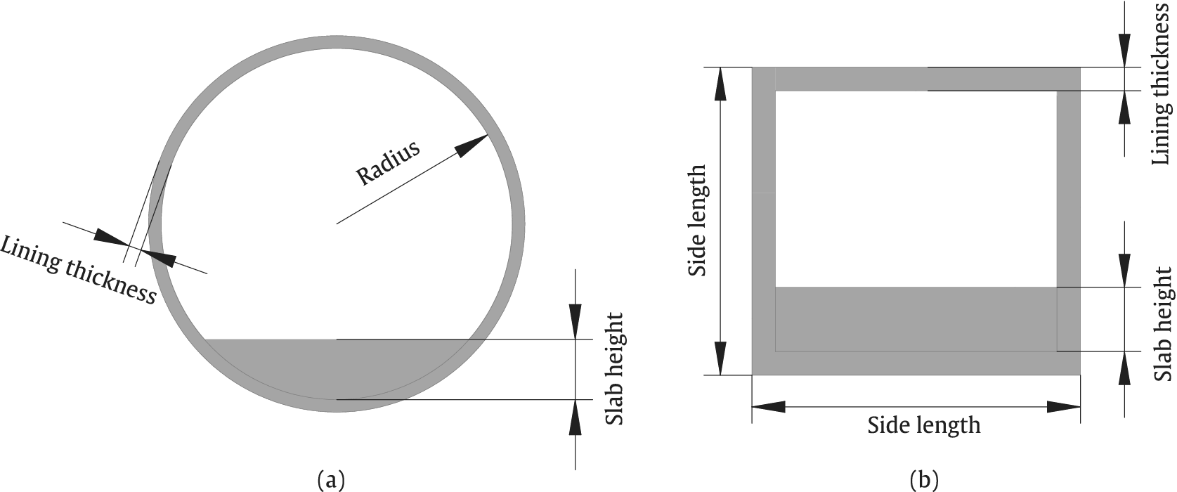
Figure 3. Schematic representation of underground railway tunnel with circular (a) and rectangular (b) cross-sections.
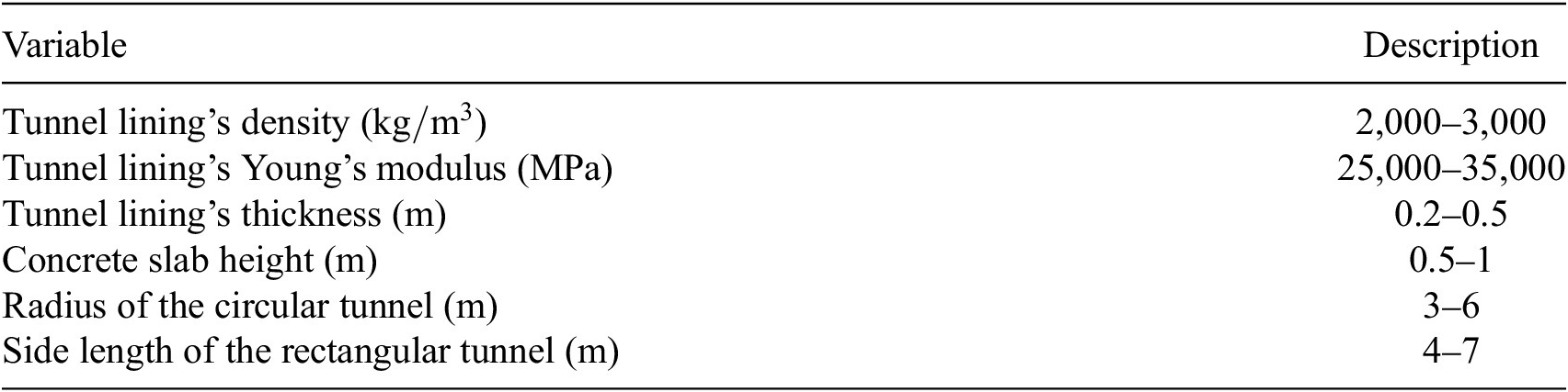
The range for the variation of each parameter in the parametric study is provided in Table 1. It is important to note that the selected parameter ranges fall within the realistic geometrical and mechanical properties of underground railway tunnels (Gupta et al., Reference Gupta, Stanus, Lombaert and Degrande2009; Ruiz et al., Reference Ruiz, Soares, Costa and Connolly2019; He et al., Reference He, Zhou and Guo2020). It is crucial to represent these parameters in the learning database in a balanced and systematic manner to prevent misleading results, such as overestimations or underestimations. To achieve this balance, the LHS technique is employed to generate input parameters. The primary aim of utilizing LHS is to reduce the number of simulations required while ensuring that the results remain reasonable and reliable (Iordanis et al., Reference Iordanis, Koukouvinos and Silou2025). In this investigation, 300 samples are utilized for training, as increasing the sample size beyond this point did not result in a significant improvement in the model’s accuracy. It should be noted that 80% of the samples are used for training, while the remaining 20% are allocated to validation. Preprocessing the data ensures that all variables are given equal importance during the training process, as discrepancies in the distributions of input parameters can lead to biases in the model, favoring features with larger values or variances. Furthermore, preprocessing enhances the speed and efficiency of the learning process. In this study, input parameters have been preprocessed using normalization, whereby the data are scaled to fall within a range of 0–1 using the following equation:
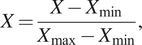 $$ X=\frac{X-{X}_{\mathrm{min}}}{X_{\mathrm{max}}-{X}_{\mathrm{min}}}, $$
where $ {X}_{\mathrm{min}} $
and
$ {X}_{\mathrm{min}} $
and $ {X}_{\mathrm{max}} $
represent the minimum and maximum values of the input parameters, respectively.
$ {X}_{\mathrm{max}} $
represent the minimum and maximum values of the input parameters, respectively.
Table 1. Ranges of variation of each parameter for the surrogate model
In this study, a random forest (RF) model is employed to develop the surrogate method based on the dataset generated using the 2.5D FEM–SBM approach (Liravi, Reference Liravi2022, Reference Liravi, Arcos and Clot-Razquin2023) for predicting displacement and traction fields. RF is a regression machine learning model, primarily composed of an ensemble of randomized decision trees, denoted as $ {\left\{f\left(x;{\Theta}_t^{(i)},{R}_n\right)\right\}}_{1\le i\le T} $
. The sequence
$ {\left\{f\left(x;{\Theta}_t^{(i)},{R}_n\right)\right\}}_{1\le i\le T} $
. The sequence $ {\left\{{\Theta}_t^{(i)}\right\}}_{1\le i\le T} $
encapsulates the random variables
$ {\left\{{\Theta}_t^{(i)}\right\}}_{1\le i\le T} $
encapsulates the random variables $ \Theta $
that govern the probabilistic mechanism underlying the construction of each tree. For a finite number of trees,
$ \Theta $
that govern the probabilistic mechanism underlying the construction of each tree. For a finite number of trees, $ T $
, the RF estimate can be expressed as follows:
$ T $
, the RF estimate can be expressed as follows:
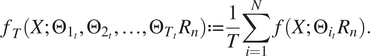 $$ {f}_T\left(X;{\Theta}_{1_t},{\Theta}_{2_t},\dots, {\Theta}_{T_t}{R}_n\right):= \frac{1}{T}\sum \limits_{i=1}^N\;f\left(X;{\Theta}_{i_t}{R}_n\right). $$
The RF model uses a least-squares boosting algorithm with 300 boosting iterations and a learning rate of 0.05. Additionally, the minimum number of samples required in a leaf node of the tree is set to 10, and the maximum number of splits allowed in a tree is set to 30. The least-squares algorithm selects several bootstrap samples, $ \left({R}_n^{\Theta_{1_t}},\dots, {R}_n^{\Theta_{T_t}}\right) $
, and applies the previous tree-based decision algorithm to these samples to construct a collection of T prediction trees. It should be noted that the 2.5D FEM–SBM approach has been thoroughly validated in a previous study, which ensures the reliability of the synthetic datasets (Liravi, Reference Liravi2022). The framework for using RF regression for prediction is illustrated in Figure 4.
$ \left({R}_n^{\Theta_{1_t}},\dots, {R}_n^{\Theta_{T_t}}\right) $
, and applies the previous tree-based decision algorithm to these samples to construct a collection of T prediction trees. It should be noted that the 2.5D FEM–SBM approach has been thoroughly validated in a previous study, which ensures the reliability of the synthetic datasets (Liravi, Reference Liravi2022). The framework for using RF regression for prediction is illustrated in Figure 4.
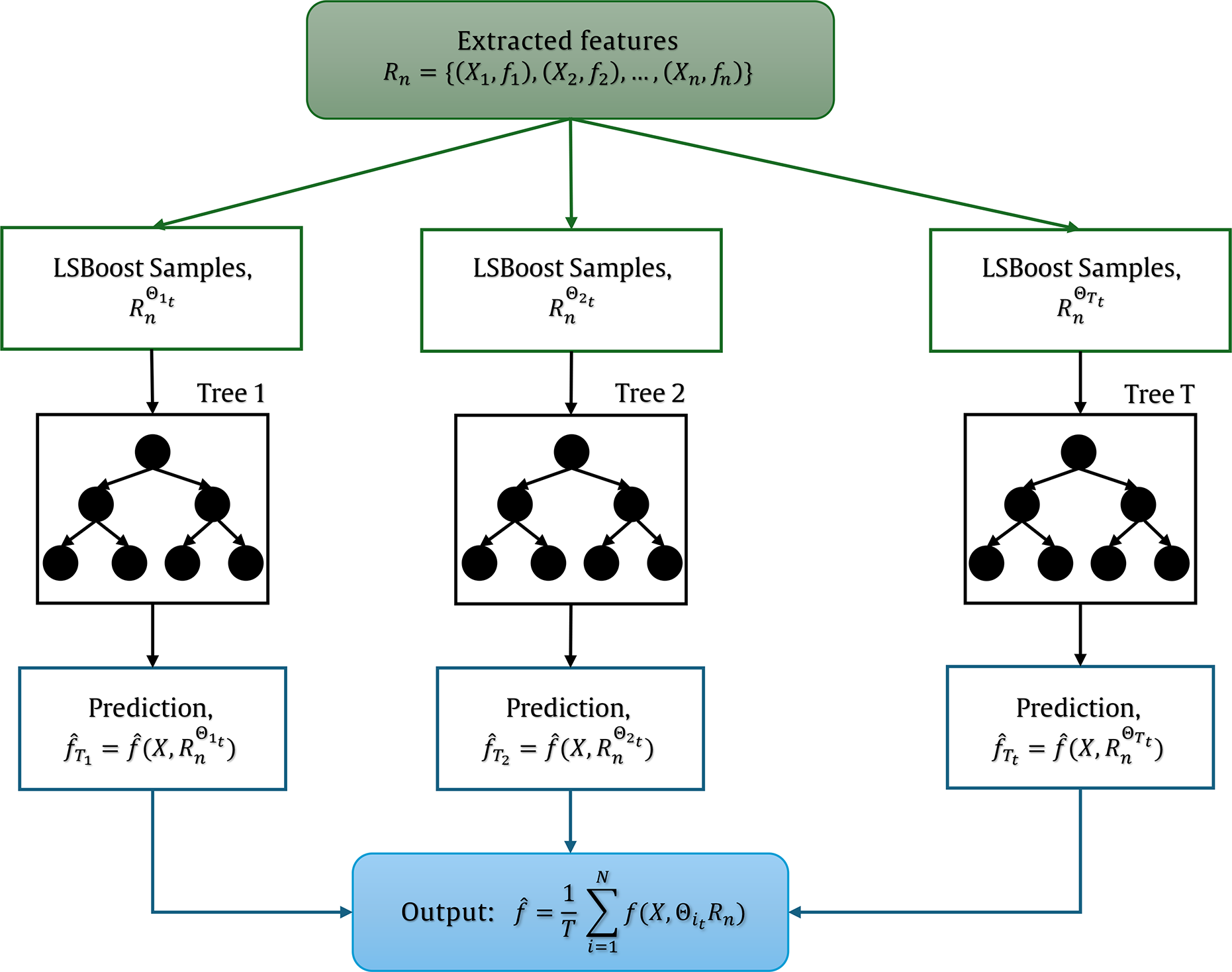
Figure 4. Illustration of Random forest regression construction.
The developed surrogate model is validated through two examples: a circular and a rectangular railway tunnel, both embedded in a homogeneous full space. Two sets of evaluation points, designated as point A and point B, are defined in the ground, as shown in Figures 5a and 9a. The geometrical and material properties of the tunnel structure are randomly selected from the validation datasets. The target outputs of the surrogate model are the displacement and traction values at the evaluation points, while the receptances and traction transfer function (TTF) values are subsequently calculated using Eq. (2.4). The results obtained by the surrogate model are compared to the 2.5D FEM–SBM approach. The comparison is made up to 80 Hz, as railway-induced ground-borne vibrations within the frequency range of 1–80 Hz can be perceived by the human body (He et al., Reference He, Zhou and Guo2022). In all simulations, the number of collocation or boundary points along the tunnel boundary is chosen to ensure a minimum of 10 nodes per shear wavelength, based on the maximum frequency of interest, thereby ensuring accurate results (Liravi, Reference Liravi2022). In all calculations conducted in this study, receptance and TTF have been computed numerically with a total of 257 sampling points, consisting of $ {k}_x=0 $
and a logarithmically spaced vector of wavenumbers ranging from
$ {k}_x=0 $
and a logarithmically spaced vector of wavenumbers ranging from $ {10}^{-3} $
to
$ {10}^{-3} $
to $ {10}^2 $
rad/m. Due to the symmetries of the displacements and tractions in the wavenumber–frequency domain caused by a vertical load, the
$ {10}^2 $
rad/m. Due to the symmetries of the displacements and tractions in the wavenumber–frequency domain caused by a vertical load, the $ x $
components of the receptances and TTF for this direction are null at
$ x $
components of the receptances and TTF for this direction are null at $ x=0 $
(Liravi, Reference Liravi2022). The results of the receptances and the TTFs are presented in decibels (dB), with references of
$ x=0 $
(Liravi, Reference Liravi2022). The results of the receptances and the TTFs are presented in decibels (dB), with references of $ {10}^{-12} $
m/N and 1 (N/m
$ {10}^{-12} $
m/N and 1 (N/m $ {}^2 $
)/N, respectively.
$ {}^2 $
)/N, respectively.
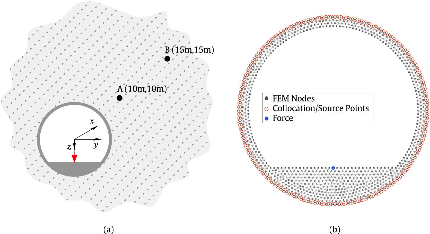
Figure 5. Schematic view of the example (a) and the FEM mesh for the circular tunnel (b). The FEM nodes, the collocation/source nodes, and the position of the applied forces used in the case study are also included.
The accuracy of the surrogate model is evaluated by calculating the relative root-mean-square error (rRMSE) with respect to a reference solution. The relative error is computed using the following expression:
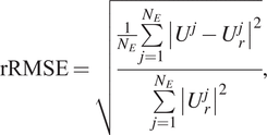 $$ \mathrm{rRMSE}=\sqrt{\frac{\frac{1}{N_E}\sum \limits_{j=1}^{N_E}{\left|{U}^j-{U}_r^j\right|}^2}{\sum \limits_{j=1}^{N_E}{\left|{U}_r^j\right|}^2}}, $$
where $ j $
is the index representing the evaluation points and
$ j $
is the index representing the evaluation points and $ {N}_E $
is the total number of evaluation points considered in the calculation. Here,
$ {N}_E $
is the total number of evaluation points considered in the calculation. Here, $ {U}^j $
and
$ {U}^j $
and $ {U}_r^j $
denote the receptances at the
$ {U}_r^j $
denote the receptances at the $ j $
th evaluation point, calculated using the assessed method and the reference method, respectively. It should be noted that the rRMSE plots are only presented for receptance values, as these will later be utilized in the optimization algorithm in the application example.
$ j $
th evaluation point, calculated using the assessed method and the reference method, respectively. It should be noted that the rRMSE plots are only presented for receptance values, as these will later be utilized in the optimization algorithm in the application example.
3.1. Underground railway tunnel with circular cross-section
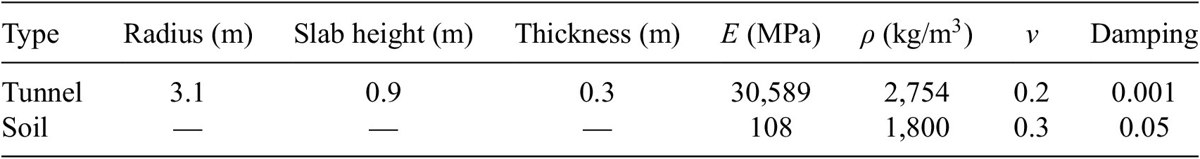
Circular cross-section tunnels are commonly used in deep tunneling due to their uniform structural force distribution, effective load-bearing capacity, and ease of shield construction. In this section, the performance of the developed surrogate model is assessed in the context of a circular tunnel embedded in a homogeneous full space. The mechanical and geometrical parameters of the tunnel and soil are presented in Table 2. The FEM mesh associated with this particular example is shown in Figure 5b.
Table 2. Mechanical parameters of the circular tunnel and the soil
As illustrated in Figure 6, there is good agreement between the receptances obtained by the developed model and those from the reference, 2.5D FEM–SBM approach, both in the $ y $
- and
$ y $
- and $ z $
-directions and at two evaluation points, with differences of up to 1 dB. However, slightly larger discrepancies are observed at point A responses in the
$ z $
-directions and at two evaluation points, with differences of up to 1 dB. However, slightly larger discrepancies are observed at point A responses in the $ y $
-direction, with differences reaching up to 2 dB. This good agreement is also evident in the TTF responses as indicated in Figure 7. The comparison against the 2.5D FEM–SBM results indicates that the surrogate model is an accurate tool for predicting both receptances and TTFs.
$ y $
-direction, with differences reaching up to 2 dB. This good agreement is also evident in the TTF responses as indicated in Figure 7. The comparison against the 2.5D FEM–SBM results indicates that the surrogate model is an accurate tool for predicting both receptances and TTFs.
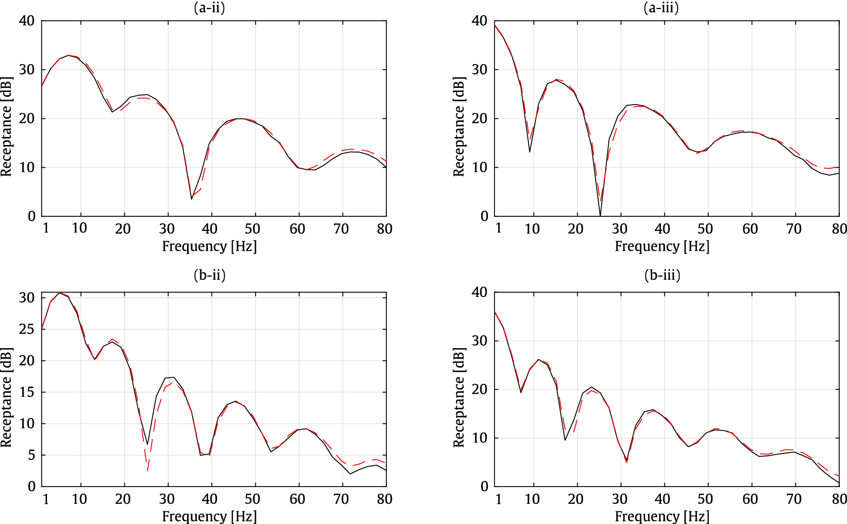
Figure 6. Receptances at points A (a) and B (b) for the y- (ii) and z- (iii) directions. Methods: 2.5D FEM–SBM (dashed red line) and surrogate model (solid black line).
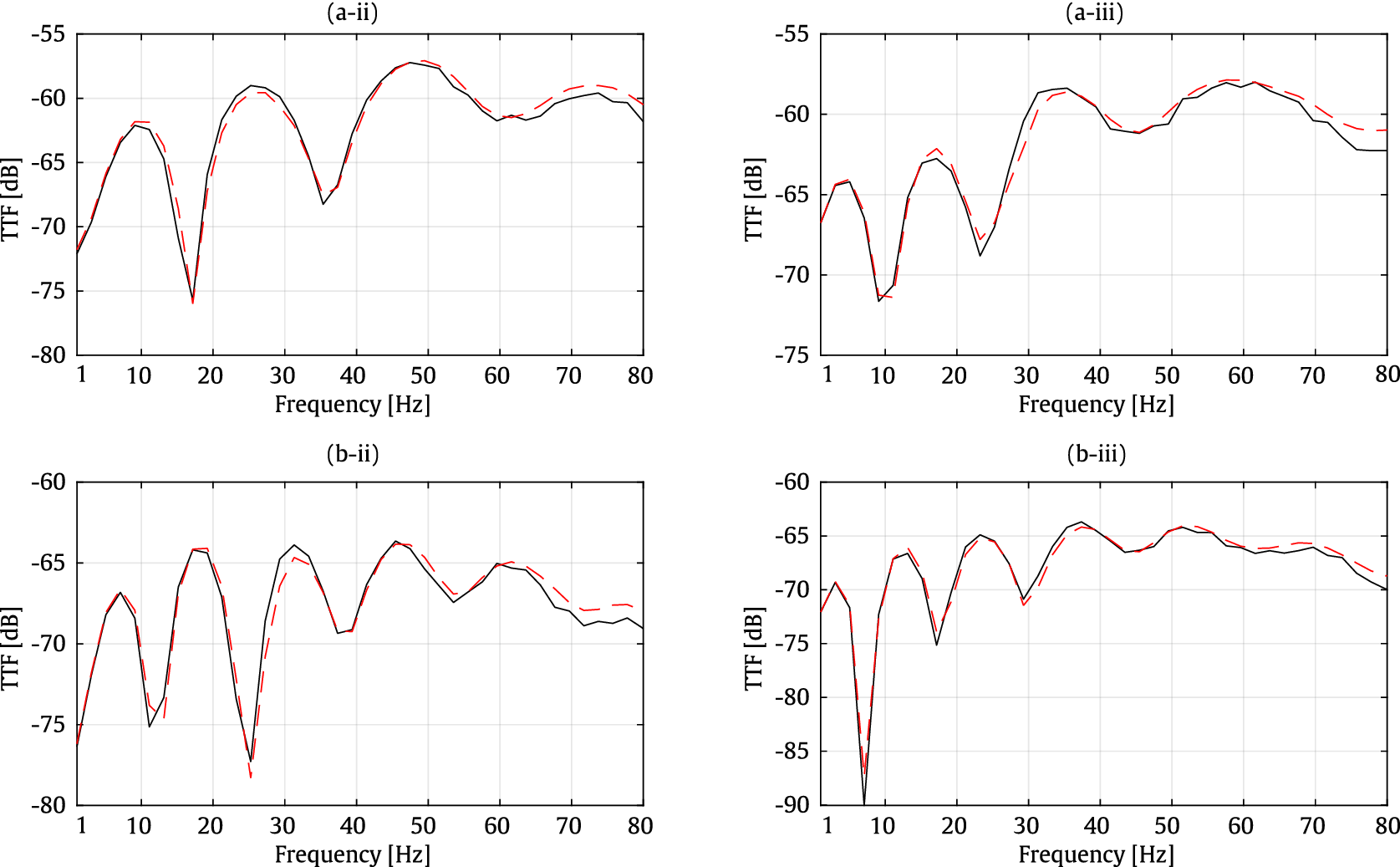
Figure 7. Traction transfer functions at points A (a) and B (b) for the y- (ii) and z- (iii) directions. Methods: 2.5D FEM–SBM (dashed red line) and surrogate model (solid black line).
The rRMSE of the receptance values is plotted in Figure 8. As shown in this figure, the rRMSE values are generally low, with an average error of approximately 3% within the considered frequency range, reaching as low as 0.2% at lower frequencies. However, at some specific frequencies, slightly higher rRMSE values are observed, particularly at the positions of the resonant/anti-resonant frequencies. Nevertheless, as mentioned earlier, the average maximum error, when compared to the 2.5D FEM–SBM approach used as the reference solution, is approximately 2 dB.
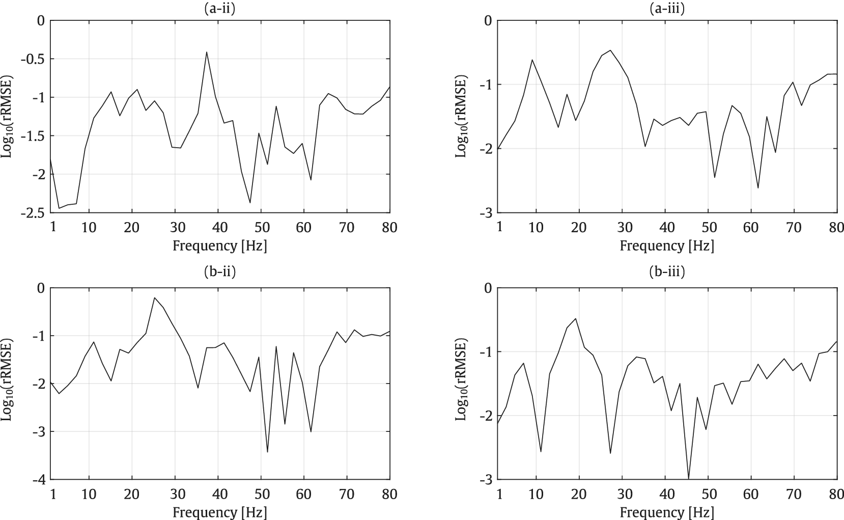
Figure 8. rRMSE of Receptances at points A (a) and B (b) for the y- (ii) and z- (iii) directions for the underground tunnel with a circular cross-section.
3.2. Underground railway tunnel with rectangular cross-section
In this section, the accuracy of the developed model is compared to the reference method, in the framework of a rectangular underground tunnel embedded in a homogenous full space. The FEM mesh used for the numerical calculations of this example and the evaluation points in the soil are presented in Figure 9. The mechanical and geometrical properties of the tunnel and soil are presented in Table 3.
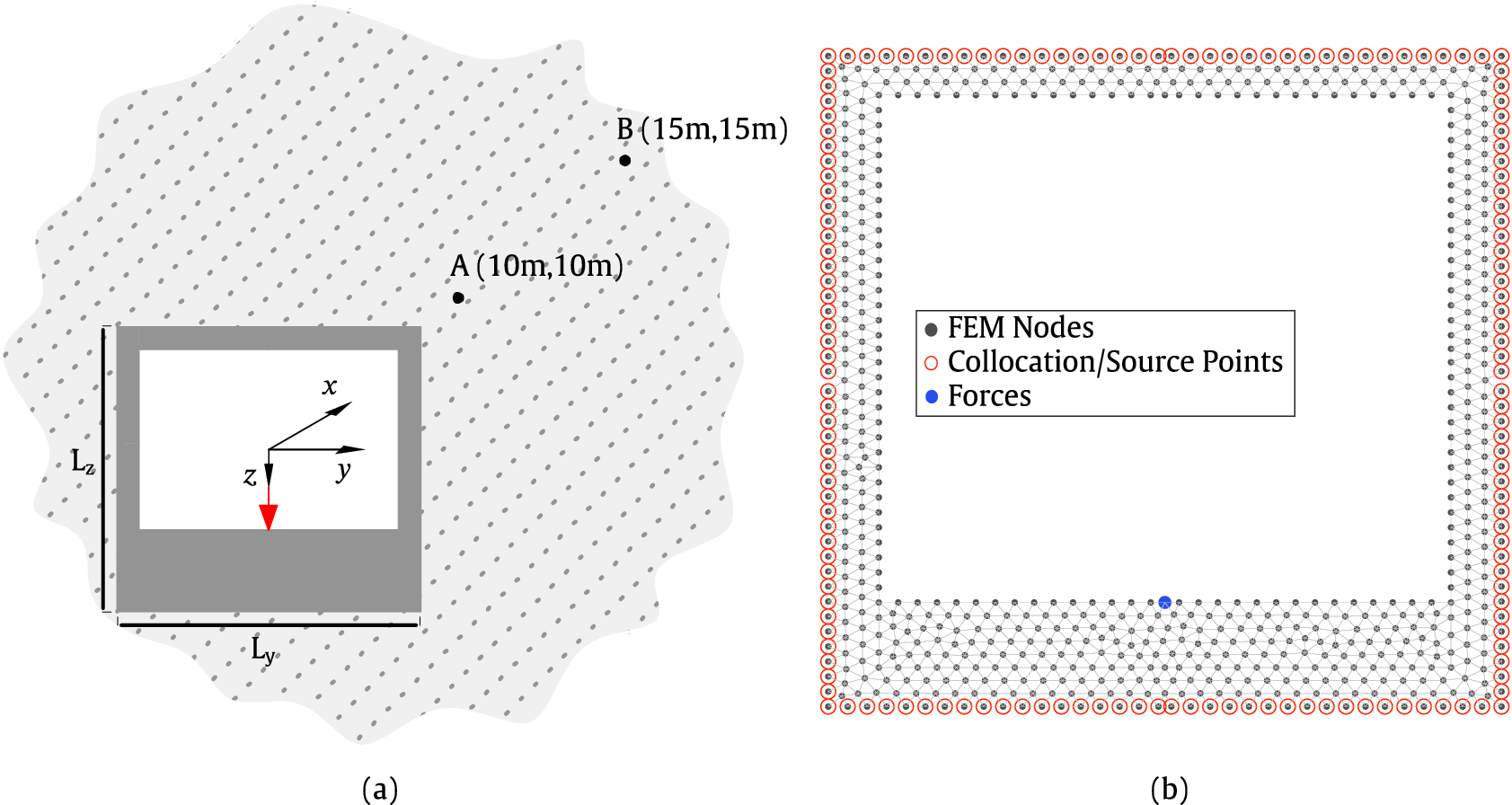
Figure 9. Schematic view of the example (a) and the FEM mesh for rectangular tunnel (b). The FEM nodes, the collocation/source nodes, and the position of the applied forces used in the case study are also included.
Table 3. Mechanical parameters of the rectangular tunnel and the soil
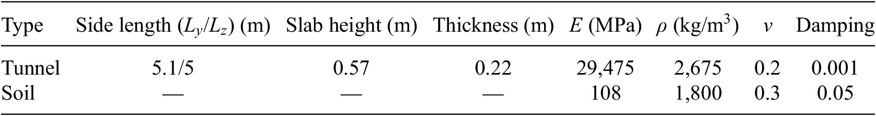
As demonstrated in Figure 10, the receptances obtained by the developed surrogate model are in good agreement when compared to the reference. A maximum of 3 dB differences can be observed, particularly at the location of the trough in the receptance trend. This good accuracy is also observed in the TTF responses, where, as shown in Figure 11, errors of up to 2 dB can be seen at specific locations on the trend. Overall, the proposed method demonstrates accurate results for the case of a railway tunnel with a rectangular cross-section.
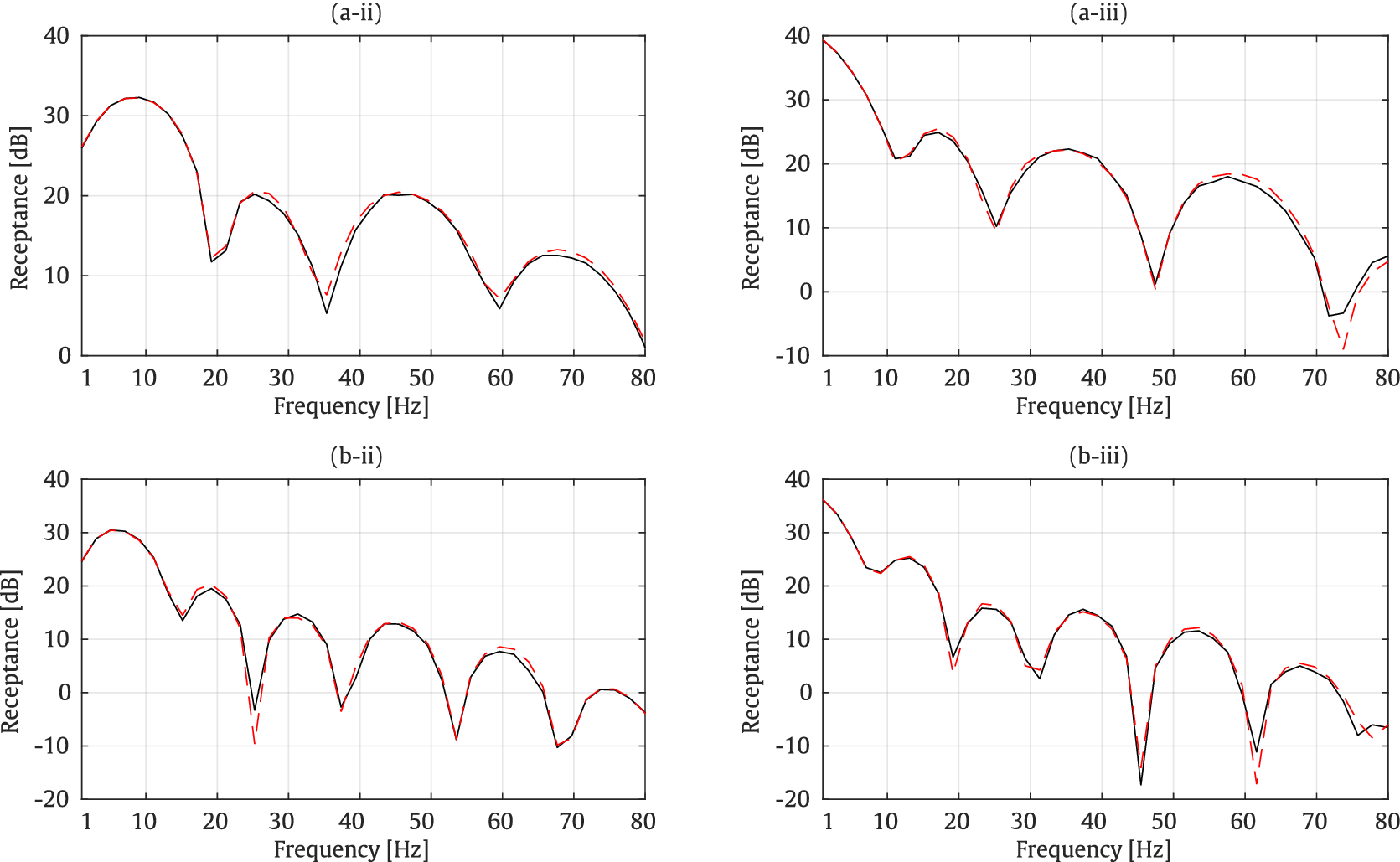
Figure 10. Receptances at points A (a) and B (b) for the y- (ii) and z- (iii) directions. Methods: 2.5D FEM–SBM (dashed red line) and surrogate model (solid black line).
Figure 11. Traction transfer functions at points A (a) and B (b) for the y- (ii) and z- (iii) directions. Methods: 2.5D FEM–SBM (dashed red line) and surrogate model (solid black line).
For this example, the rRMSE plot of the receptance values is presented in Figure 12. As indicated, the rRMSE values are generally low, with an average error of approximately 3.5% within the considered frequency range, reaching as low as 1%, particularly at lower frequencies. However, similar to the previous example, at some specific frequencies, slightly higher rRMSE values are observed. As mentioned earlier, the maximum error does not exceed 2 dB.
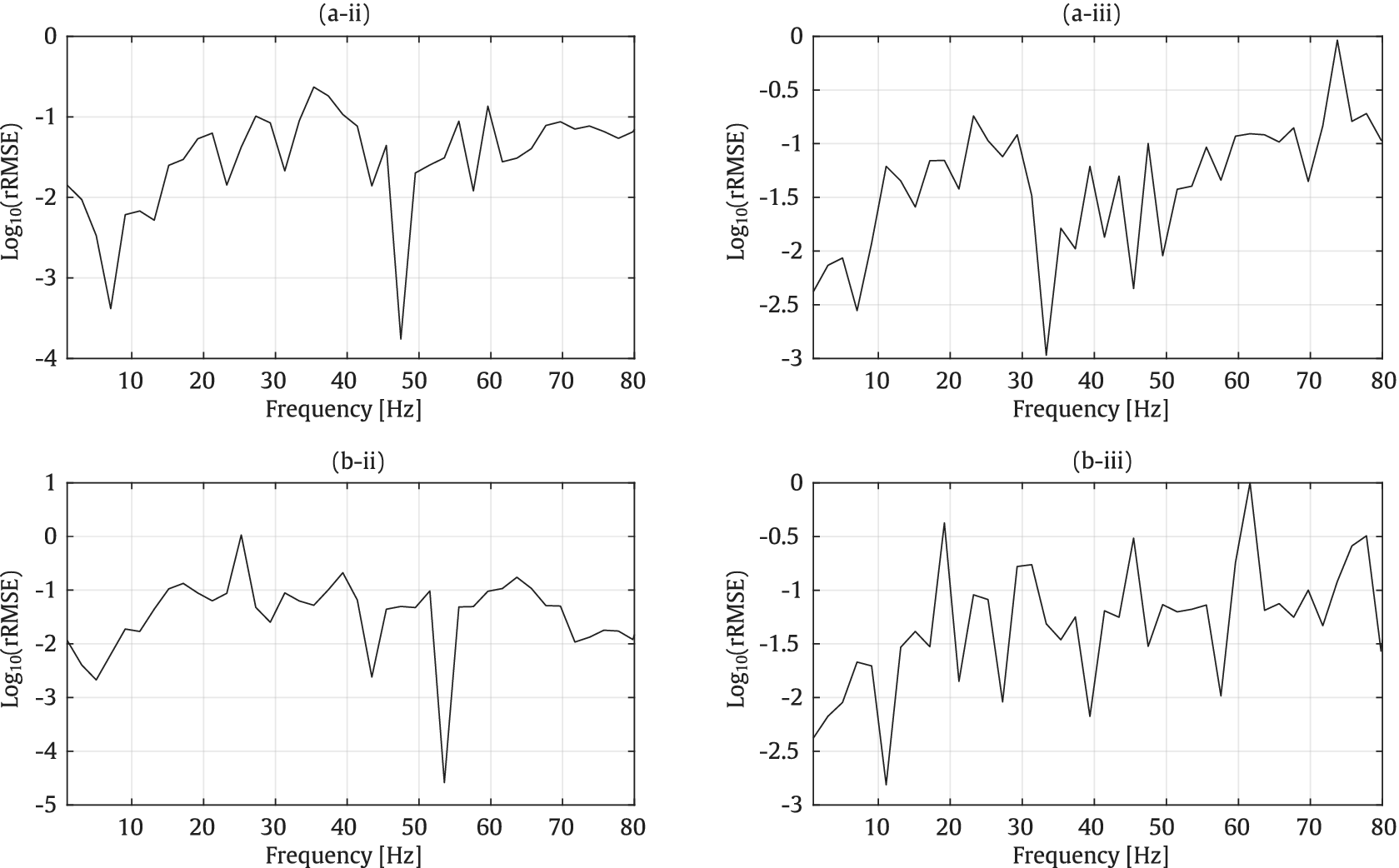
Figure 12. rRMSE of Receptances at points A (a) and B (b) for the y- (ii) and z- (iii) directions for the underground tunnel with a rectangular cross-section.
4. Optimization
This study employs a Bayesian optimization method to optimize underground railway tunnels from specific geometrical and material perspectives. As previously mentioned, the optimization is conducted within the logical ranges of the considered parameters, as indicated in Table 1. The optimization process is illustrated through two case studies involving underground railway tunnels with circular and rectangular cross-sections. It should be noted that the optimization process is conducted at a single frequency. In this study, the frequencies of 20 and $ 80\hskip0.22em \mathrm{Hz} $
are considered, representing low and high frequencies, respectively. In this section, the objective of the optimization is to minimize the vertical receptance values at the target point (point A, as illustrated in earlier examples) while simultaneously optimizing the considered geometrical and material parameters of the underground tunnel. Specifically, the five parameters used for training the surrogate model, including Young’s modulus, density, and thickness of the tunnel lining, as well as the concrete slab height and radius/side length of the tunnel, are the parameters to be optimized. Optimization iterations continue until the results converge and show no further changes. To ensure the accuracy of the optimization, each example has been run five times, and the optimal values presented are the average of these five repetitions. The optimization problem for an embedded structure in an elastic medium is defined as a classical optimization problem of the form:
$ 80\hskip0.22em \mathrm{Hz} $
are considered, representing low and high frequencies, respectively. In this section, the objective of the optimization is to minimize the vertical receptance values at the target point (point A, as illustrated in earlier examples) while simultaneously optimizing the considered geometrical and material parameters of the underground tunnel. Specifically, the five parameters used for training the surrogate model, including Young’s modulus, density, and thickness of the tunnel lining, as well as the concrete slab height and radius/side length of the tunnel, are the parameters to be optimized. Optimization iterations continue until the results converge and show no further changes. To ensure the accuracy of the optimization, each example has been run five times, and the optimal values presented are the average of these five repetitions. The optimization problem for an embedded structure in an elastic medium is defined as a classical optimization problem of the form:
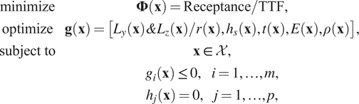 $$ {\displaystyle \begin{array}{cc}\operatorname{minimize}& \boldsymbol{\Phi} \left(\mathbf{x}\right)=\mathrm{Receptance}/\mathrm{TTF},\\ {}\mathrm{optimize}& \mathbf{g}\left(\mathbf{x}\right)=\left[{L}_y\left(\mathbf{x}\right)\&{L}_z\left(\mathbf{x}\right)/r\left(\mathbf{x}\right),{h}_s\left(\mathbf{x}\right),t\left(\mathbf{x}\right),E\left(\mathbf{x}\right),\rho \left(\mathbf{x}\right)\right],\\ {}\mathrm{subject}\ \mathrm{to}& \mathbf{x}\in \mathcal{X},\\ {}& {g}_i\left(\mathbf{x}\right)\le 0,\hskip1em i=1,\dots, m,\\ {}& {h}_j\left(\mathbf{x}\right)=0,\hskip1em j=1,\dots, p,\end{array}} $$
where $ \Phi $
represents the objective function for the optimization algorithm (in this study, receptances or the TTF),
$ \Phi $
represents the objective function for the optimization algorithm (in this study, receptances or the TTF), $ {L}_y $
and
$ {L}_y $
and $ {L}_z $
are the side lengths of the rectangular tunnel,
$ {L}_z $
are the side lengths of the rectangular tunnel, $ r $
denotes the radius of the circular tunnel,
$ r $
denotes the radius of the circular tunnel, $ {h}_s $
represents the slab height,
$ {h}_s $
represents the slab height, $ t $
denotes the thickness of the tunnel lining, and
$ t $
denotes the thickness of the tunnel lining, and $ \mathbf{x} $
is the vector of design parameters. Meanwhile,
$ \mathbf{x} $
is the vector of design parameters. Meanwhile, $ {g}_i\left(\mathbf{x}\right) $
and
$ {g}_i\left(\mathbf{x}\right) $
and $ {h}_j\left(\mathbf{x}\right) $
correspond to the inequality and equality constraints, respectively. These constraints are established based on the imposed limits on the design parameters and the elastic wave equation, as defined earlier in Eq. (2.1).
$ {h}_j\left(\mathbf{x}\right) $
correspond to the inequality and equality constraints, respectively. These constraints are established based on the imposed limits on the design parameters and the elastic wave equation, as defined earlier in Eq. (2.1).
4.1. Underground railway tunnel with circular cross-section
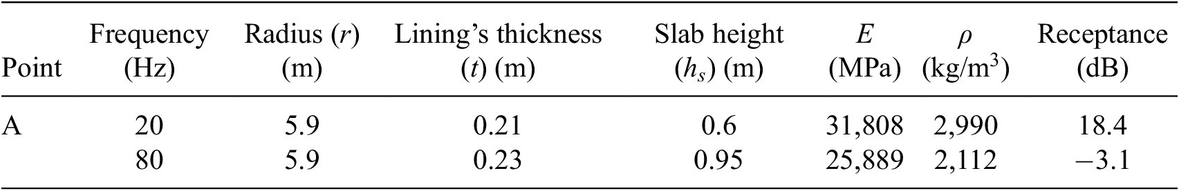
The first optimization example considers an underground railway tunnel with a circular cross-section embedded in a homogeneous full-space medium. The optimization is visualized in Figures 13 and 14 for the frequencies of 20 and 80 Hz, respectively. As shown, the geometrical parameters, including the slab height and the thickness of the tunnel, are presented in one figure, while the material parameters, such as Young’s modulus and density, are depicted together. In both figures, the minimum objective function is observed when the tunnel thickness is set between 0.2 and 0.3 m, and the slab height is greater than 0.6 m. At a frequency of 20 Hz, the minimum objective function is observed for material densities greater than 2,800 $ \mathrm{kg}/{\mathrm{m}}^3 $
and Young’s modulus between 28,000 and 33,000 MPa. For a frequency of 80 Hz, these ranges shift to 2,000–2,200
$ \mathrm{kg}/{\mathrm{m}}^3 $
and Young’s modulus between 28,000 and 33,000 MPa. For a frequency of 80 Hz, these ranges shift to 2,000–2,200 $ \mathrm{kg}/{\mathrm{m}}^3 $
for material density and 23,000–27,000 MPa for Young’s modulus, respectively.
$ \mathrm{kg}/{\mathrm{m}}^3 $
for material density and 23,000–27,000 MPa for Young’s modulus, respectively.
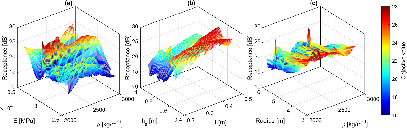
Figure 13. Optimization plot for a railway tunnel with a circular cross-section at a frequency of 20 Hz, illustrating the variations in performance across different considered parameters.
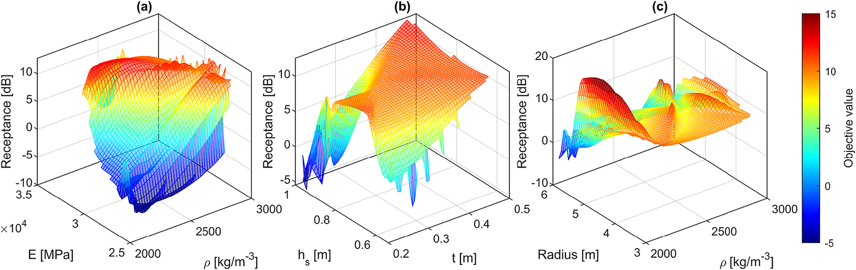
Figure 14. Optimization plot for a railway tunnel with a circular cross-section at a frequency of 80 Hz, illustrating the variations in performance across different considered parameters.
Additionally, Figures 13c and 14c show the optimization iterations between a geometrical design parameter and a mechanical property, in particular, the radius of the tunnel is plotted against its density for the frequencies of 20 and 80 Hz, respectively. At both frequencies, the minimum receptance value is observed when the largest tunnel radius is selected. The lining thickness in both cases is optimized to its minimum value. The optimal values of the parameters under consideration are provided in Table 4.
Table 4. Results of the optimization algorithm for the case of underground tunnel with circular cross-section
When comparing the vertical receptances at point A for the optimized case against a random validation example presented in Figure 6b(iii), an attenuation of approximately 8 dB in vertical receptance can be observed at both considered frequencies.
4.2. Underground railway tunnel with rectangular cross-section
The second optimization case involves an underground railway tunnel with a rectangular cross-section, similar to the previous example, embedded in a homogeneous full-space medium. In this case, as illustrated in Figures 15 and 16, the visualization of the optimization process for the side lengths of the tunnel is presented together, while the thickness of the tunnel and the slab height are displayed in a separate plot. Additionally, the material properties of the tunnel, specifically the density and Young’s modulus, are presented together. The optimal values reveal that, at a frequency of 20 Hz, the side lengths of the tunnel should be set to 6.9 and 6.5 m, with the minimum thickness within the considered range selected to minimize the vertical receptance at point A. Similarly, at a frequency of 80 Hz, $ {L}_y $
and
$ {L}_y $
and $ {L}_z $
should be set to 6.9 and 6.4 m, respectively, again with the minimum thickness within the considered range achieving the same goal. Furthermore, the optimal concrete slab height is approximately 0.9 m at both frequencies, while the density at 80 Hz is approximately 300
$ {L}_z $
should be set to 6.9 and 6.4 m, respectively, again with the minimum thickness within the considered range achieving the same goal. Furthermore, the optimal concrete slab height is approximately 0.9 m at both frequencies, while the density at 80 Hz is approximately 300 $ \mathrm{kg}/{\mathrm{m}}^3 $
lower than that at 20 Hz. The optimal values of the considered parameters across all optimization cases associated with this example are summarized in Table 5.
$ \mathrm{kg}/{\mathrm{m}}^3 $
lower than that at 20 Hz. The optimal values of the considered parameters across all optimization cases associated with this example are summarized in Table 5.
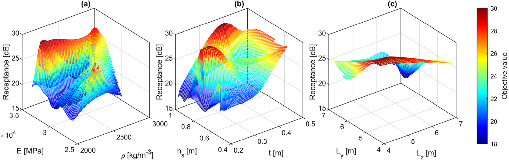
Figure 15. Optimization plot for a railway tunnel with a rectangular cross-section at a frequency of 20 Hz, illustrating the variations in performance across different considered parameters.
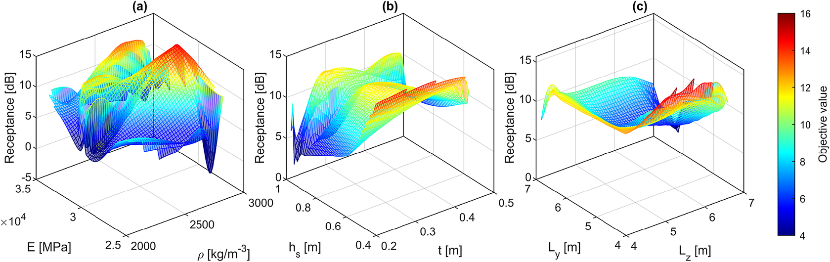
Figure 16. Optimization plot for a railway tunnel with a rectangular cross-section at a frequency of 80 Hz, illustrating the variations in performance across different considered parameters.
Table 5. Results of the optimization algorithm for the case of underground tunnel with rectangular cross-section
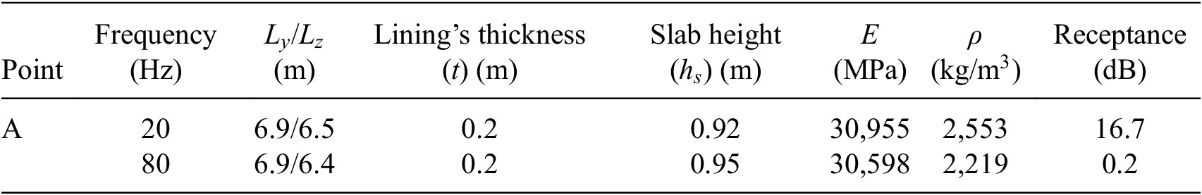
It is noteworthy that, when comparing the vertical receptance values presented in Figure 10b(iii) for a random validation case of an underground tunnel with a rectangular cross-section, an approximate reduction of 6 and 5 dB can be achieved by optimizing the tunnel from both geometrical and material perspectives, at the frequencies of 20 and 80 Hz, respectively.
5. Assessment of the performance of the optimized cases
To further highlight the differences between the optimized cases and the random validation case presented in Figures 6 and 10 across the entire frequency range, bar plots are provided in Figures 17 and 18 for the circular and rectangular tunnel cases, respectively. These plots show the receptance differences between the optimized cases and the validation case at 10-Hz intervals. The comparison considers both optimized cases at 20 and 80 Hz. In these plots, negative values indicate the extent of improvement achieved in the optimized case relative to the non-optimized case, while positive values represent a deterioration in the optimization outcomes.
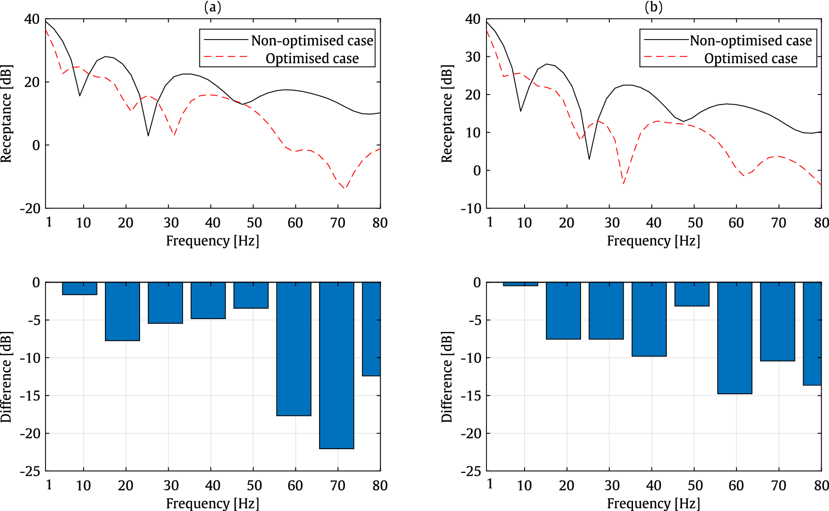
Figure 17. Comparison of vertical receptances computed at evaluation point A between the non-optimized case and optimized cases at 20 Hz (a) and 80 Hz (b), along with bar plots showing the differences between the cases in decibels for an underground tunnel with a circular cross-section.
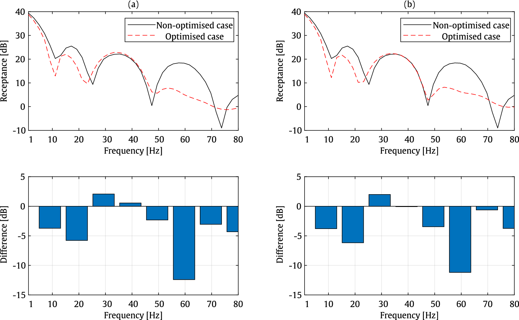
Figure 18. Comparison of vertical receptances computed at evaluation point A between the non-optimized case and optimized cases at 20 Hz (a) and 80 Hz (b), along with bar plots showing the differences between the cases in decibels for an underground tunnel with a rectangular cross-section.
For the case of an underground tunnel with a circular cross-section, a significant improvement is observed across the entire frequency range. Similarly, for the underground tunnel with a rectangular cross-section, the bar plots clearly demonstrate that the optimized cases result in improvements in vertical receptance throughout the frequency range. However, minor negative impacts of up to 2 dB are observed around 30–40 Hz.
Since the optimization process results in different design parameters for the tunnel at different frequencies, as shown in Tables 4 and 5, the design parameters can be selected based on the required target frequency, considering the problem under study. As demonstrated in this section, optimization at a specific frequency results in an improvement in the system’s performance over a wider range of frequencies.
Overall, the results indicate that the proposed optimization approach is highly effective in enhancing elastic wave propagation performance at the entire frequency range. In summary, this optimization method offers a promising tool for improving the design of buried structures, making it suitable for practical applications where mitigating elastic wave propagation is a key concern.
6. Conclusion
This study presents a surrogate model for the optimization of underground railway tunnels with respect to specific geometrical and material aspects, developed in the wavenumber–frequency domain. The validation and optimization processes are conducted in the context of underground railway tunnels with circular and rectangular cross-sections. The primary objective of the optimization algorithm is to minimize elastic wave propagation in the surrounding soil. The key findings of this research are as follows:
-
• The 2.5D FEM–SBM approach is an accurate, efficient, and robust numerical method for generating datasets for training the surrogate model. Furthermore, it effectively handles geometries that are more complex than circular tunnels, such as railway tunnels with rectangular cross-sections.
-
• The developed surrogate model demonstrates a high degree of accuracy in responses obtained at evaluation points when compared to the reference method, with an average rRMSE of receptances of approximately 3% and 3.5% observed within the considered frequency range for the examples of underground railway tunnels with circular and rectangular cross-sections, respectively. This precision is also evident in the TTF responses when compared to the reference method.
-
• The optimization case of an underground railway tunnel with a circular cross-section indicates that by optimizing specific geometrical and material perspectives of the underground tunnel structure, the vertical receptances at an arbitrary evaluation point in the soil, approximately near the tunnel, can be significantly mitigated. For the specific example presented in this study, an average reduction of 10 dB is observed in the target frequencies.
-
• The optimization example of an underground railway tunnel with a rectangular cross-section also provides promising results. For the specific case presented in this study, an average attenuation of 6 dB in vertical receptances can be achieved by optimizing the tunnel shape and material properties at target frequencies.
As a limitation, the optimization algorithm must be carried out based on the target frequency, although it may also demonstrate improvements at other frequencies, as evidenced by the results presented in this paper. Furthermore, the model could be improved and extended in future work to incorporate both frequency and wavenumber as inputs for the surrogate model. This enhancement would lead to a significantly faster training process and reduced storage requirements. Overall, the optimization algorithm, combined with the surrogate model, proves to be a suitable prediction and optimization toolbox for addressing tunnel–soil interaction problems in elastodynamics. However, it should be noted that the current study has been implemented and developed exclusively for a homogeneous full-space soil medium. To achieve greater realism, the model should also consider a horizontally layered half-space medium.
Data availability statement
Replication data will be found in GitHub of Meta-NOVIB project (https://github.com/HassanLiravi/Meta-NOVIB) and on Zenodo (https://doi.org/10.5281/zenodo.15491461) Liravi (Reference Liravi2025).
Acknowledgements
H.L. would like to express deep gratitude for the support provided by the Laboratori d’Enginyeria Acústica i Mecànica (LEAM) of the Universitat Politècnica de Catalunya (UPC).
Author contribution
Conceptualization: H.L., J.N.; Data curation: H.L.; Data visualization: H.L.; Methodology: H.L., J.N.; Writing—original draft: H.L., H.G.B.; Writing—review and editing: J.N., A.C., S.K. All authors approved the final submitted draft.
Funding statement
This project has received funding from the UKRI Horizon Europe Underwriting—EPSRC for guaranteeing the Marie Sklodowska-Curie Grant Agreement Number EP/Z001129/1 “META-NOVIB: Digital twin for ground-borne railway-induced NOise and VIBration control with METAmaterials in underground tunnels.” This support is gratefully acknowledged. Additionally, A.C. would like to acknowledge the financial support by Base Funding—UIDB/04708/2020 with DOI 10.54499/UIDB/04708/2020 (https://doi.org/10.54499/UIDB/04708/2020) and Programmatic Funding—UIDP/04708/2020 with DOI 10.54499/UIDP/04708/2020 (https://doi.org/10.54499/UIDP/04708/2020) of the CONSTRUCT—Instituto de I&D em Estruturas e Construções—funded by national funds through the FCT/MCTES (PIDDAC); Project PTDC/ECI-EGC/3352/2021, funded by national funds through FCT/MCTES; Individual Grant No. 2022.00898 CEECIND (Scientific Employment Stimulus—5th Edition) provided by FCT (https://doi.org/10.54499/2022.00898.CEECIND/CP1733/CT0005).
Competing interests
The authors declare no competing interests.
Ethical standard
The research meets all ethical guidelines, including adherence to the legal requirements of the study country.


 Open access
Comments
No Comments have been published for this article.