


Impact Statement
The methodology we present in this article can be applied to a wide range of problems involving sequential decision making. As presented in a water leak detection experiment, one may apply the algorithm to guide robots in automated monitoring of underground water lines. Other applications include environmental monitoring, chemical synthesis, disease control, and so forth. One of the main advantages of the proposed framework when compared to previous Bayesian optimization approaches is the interpretability of the model, which allows for inferring variables important for analysis and decision support. In addition, practical performance improvements are also observed in experiments.
1. Introduction
Bayesian optimization (BO) offers a principled approach to integrate probabilistic models into processes of decision making under uncertainty (Shahriari et al., Reference Shahriari, Swersky, Wang, Adams and De Freitas2016). In particular, BO has been successful in optimization problems involving black-box functions and very little prior information, such as smoothness of the objective function. Examples include hyperparameter tuning (Snoek et al., Reference Snoek, Larochelle, Adams, Pereira, Burges, Bottou and Weinberger2012), robotic exploration (Souza et al., Reference Souza, Marchant, Ott, Wolf and Ramos2014), and chemical design (Shields et al., Reference Shields, Stevens, Li, Parasram, Damani, Alvarado, Janey, Adams and Doyle2021), and disease control (Spooner et al., Reference Spooner, Jones, Fearnley, Savani, Turner and Baylis2020). Most of its success relies on the flexibility and well-understood properties of nonparametric modeling frameworks, particularly Gaussian process (GP) regression (Rasmussen and Williams, Reference Rasmussen and Williams2006). Although nonparametric models are usually the best approach for problems with scarce prior information, they offer little in terms of interpretability and may be a suboptimal guide when compared to expert parametric models. In these expert models, parameters are attached to variables with physical meaning and reveal aspects of the nature of the problem, since models are derived from domain knowledge.
As a motivating example, consider the problem of localizing leaks in underground water distribution pipes (Mashford et al., Reference Mashford, De Silva, Burn and Marney2012). Measurements from pipe monitoring stations are usually sparse and excavations are costly (Sadeghioon et al., Reference Sadeghioon, Metje, Chapman and Anthony2014). As a possible alternative, microgravimetric sensors have recently allowed detecting gravity anomalies of parts in a billion (Brown et al., Reference Brown, Ridley, Rodgers and de Villiers2016; Hardman et al., Reference Hardman, Everitt, McDonald, Manju, Wigley, Sooriyabandara, Kuhn, Debs, Close and Robins2016), making them an interesting data source for subsurface investigations (Hauge and Kolbjørnsen, Reference Hauge and Kolbjørnsen2015; Rossi et al., Reference Rossi, Reguzzoni, Sampietro and Sansò2015). One could then design a GP-based BO algorithm to localize a leak in a pipe by searching for a maximum in the gravity signal on the surface due to the heavier wet soil. The determined 2D location, however, tells nothing of the depth or the volume of leaked water. In this case, a physics-based probabilistic model of a simulated water leak could better guide BO and the decision-making end users. Bayesian inference on complex parametric models, however, is usually intractable, requiring the use of sampling-based techniques, like Markov chain Monte Carlo (MCMC) (Andrieu et al., Reference Andrieu, De Freitas, Doucet and Jordan2003), or variational inference methods (Bishop, Reference Bishop2006; Ranganath et al., Reference Ranganath, Gerrish and Blei2014). Either of these approaches can lead to high computational overheads during the posterior updates in a BO loop.
In this article, we investigate a relatively unexplored modeling approach in the BO community which offers a balanced trade-off between MCMC and approximate inference methods for problems where domain knowledge is available. Namely, we consider sequential Monte Carlo (SMC) (Doucet et al., Reference Doucet, de Freitas and Gordon2001), also known as particle filtering, algorithms as posterior update mechanisms for BO. SMC has an accuracy-speed trade-off controlled by the number of particles it uses, and it suffers less of the drawbacks of other approximate inference methods (Bishop, Reference Bishop2006), while still enjoying asymptotic convergence guarantees similar to MCMC (Crisan and Doucet, Reference Crisan and Doucet2002; Beskos et al., Reference Beskos, Crisan, Jasra and Whiteley2014). SMC methods have traditionally been applied to state-space models for localization (Thrun et al., Reference Tran, Scharth, Gunawan, Kohn, Brown and Hawkins2006) and tracking (Doucet et al., Reference Doucet, Godsill and Andrieu2000) problems, but SMC has also found use in more general areas, including experimental design (Kuck et al., Reference Kuck, de Freitas and Doucet2006) and likelihood-free inference (Sisson et al., Reference Sisson, Fan and Tanaka2007).
As contributions, we present an approach to efficiently incorporate SMC within BO frameworks. In particular, we derive an acquisition function to take advantage of the flexibility of SMC’s particle distributions by means of empirical quantile functions. Our approach compensates for the approximation bias in the empirical quantiles by taking into account SMC’s effective sample size (ESS). We also propose methods to reduce the correlation and bias among SMC samples and improve its predictive power. Lastly, experimental results demonstrate practical performance improvements over GP-based BO approaches.
2. Related Work
Other than the GP approach, BO frameworks have applied a few other methods for surrogate modeling, including linear parametric models with nonlinear features (Snoek et al., Reference Snoek, Rippel, Swersky, Kiros, Satish, Sundaram, Patwary and Adams2015), Bayesian neural networks (Springenberg et al., Reference Srinivas, Krause, Kakade and Seeger2016), and random forests (Hutter et al., Reference Hutter, Hoos and Leyton-Brown2011). Linear models and limits of Bayesian neural networks when the number of neurons approaches infinity can be directly related to GPs (Rasmussen and Williams, Reference Rasmussen and Williams2006; Khan et al., Reference Khan, Immer, Abedi and Korzepa2019). Mostly these approaches, however, consider a black-box setting for the optimization problem, where very little is known about the stochastic process defining the objective function. In this article, we take BO instead toward a gray-box formulation, where we know a parametric structure which can accurately describe the objective function, but whose true parameters are unknown.
SMC has previously been combined with BO in GP-based approaches. Benassi et al. (Reference Benassi, Bect, Vazquez, Hamadi and Schoenauer2012) applies SMC to the problem of learning the hyperparameters of the GP surrogate during the BO process by keeping and updating a set of candidate hyperparameters according to the incoming observations. Bijl et al. (Reference Bijl, Schön, van Wingerden and Verhaegen2016) provide a method for Thompson sampling (Russo and Van Roy, Reference Russo and Van Roy2016) using SMC to keep track of the distribution of the global optimum. These approaches still use GPs as the main modeling framework for the objective function. Lastly and more related to this article, Dalibard et al. (Reference Dalibard, Schaarschmidt and Yoneki2017) presents an approach to use SMC for inference with semiparametric models, where one combines GPs with informative parametric models. Their framework is tailored to automatically tuning computer programs following dynamical systems, where the system state transitions. In contrast, our approach is based on a static formulation of SMC, where the system state corresponds to a probabilistic model’s parameters vector, which does not change over time. Simply adapting a dynamics-based SMC model to a static system is problematic due to particle degeneracy in the lack of a transition model (Doucet et al., Reference Doucet, Godsill and Andrieu2000). We instead apply MCMC to move and rejuvenate particles in the static SMC framework, as originally proposed by Chopin (Reference Chopin2002).
In the multiarmed bandits literature, whose methods have frequently been applied to BO (Srinivas et al., Reference Szörényi, Busa-Fekete, Weng and Hüllermeier2010; Wang and Jegelka, Reference Young and Freedman2017; Berkenkamp et al., Reference Berkenkamp, Schoellig and Krause2019), SMC has also been shown as a useful modeling framework (Kawale et al., Reference Kawale, Bui, Kveton, Thanh and Chawla2015; Urteaga and Wiggins, Reference Urteaga and Wiggins2018). In particular, Urteaga and Wiggins (Reference Urteaga and Wiggins2018) present a SMC approach to bandits in dynamic problems, where the reward function evolves over time. A generalization of their approach has recently been proposed to include linear and discrete reward functions (Urteaga and Wiggins, Reference Wand and Jones2019) with support by empirical results. Bandit problems seek policies which maximize long-term payoffs. In this article, we instead focus on investigating and addressing the effects of the SMC approximation on a more general class of problems. We also provide experimental results on applications where domain knowledge offers informative models.
Lastly, BO algorithms provide model-based solutions for black-box derivative-free optimization problems (Rios and Sahinidis, Reference Rios and Sahinidis2013). In this context, there are plenty of other model-free approaches, such as evolutionary algorithms, which include the popular covariance matrix adaptation evolution strategy (CMA-ES) algorithm (Arnold and Hansen, Reference Arnold and Hansen2010). However, these approaches are usually not focused on improving data efficiency as the usually require hundreds or even thousands of steps to converge to a global optimum. In contrast, BO algorithms are usually applied to problems where the number of evaluations of the objective function is very limited, usually to the order of tens of evaluations, due to a high cost of collecting observations (Shahriari et al., Reference Shahriari, Swersky, Wang, Adams and De Freitas2016), for example, drilling a hole to find natural gas deposits. The algorithm we propose in this article also targets this kind of use case, with the difference that we apply more informative predictive models than the usual GP-based formulations.
3. Preliminaries
In this section, we specify our problem setup and review relevant theoretical background. We consider an optimization problem over a function  $ f:\mathcal{X}\to \unicode{x211D} $ within a compact search space $ \mathcal{S}\subset \mathcal{X}\subseteq {\unicode{x211D}}^d $:
 $$ {\mathbf{x}}^{\ast}\in \hskip0.2em \underset{\mathbf{x}\in \mathcal{S}}{\mathrm{argmax}}\hskip0.2em f\left(\mathbf{x}\right). $$
We assume a parametric formulation for  $ f\left(\mathbf{x}\right)=h\left(\mathbf{x},\theta \right) $, where $ h:\mathcal{X}\times \Theta \to \unicode{x211D} $ has a known form, but $ \boldsymbol{\theta} \in \Theta \subset {\unicode{x211D}}^m $ is an unknown parameter vector. The only prior information about $ \boldsymbol{\theta} $ is a probability distribution $ p\left(\boldsymbol{\theta} \right) $. We are allowed to collect up to $ T $ observations $ {o}_t $ distributed according to an observation (or likelihood) model $ p\left({o}_t|\boldsymbol{\theta}, {\mathbf{x}}_t\right) $, for $ t\in \left\{1,\dots, T\right\} $. For instance, in the classical white Gaussian noise setting, we have $ {o}_t=f\left({\mathbf{x}}_t\right)+{\varepsilon}_t $, with $ {\varepsilon}_t\sim \mathcal{N}\left(0,{\sigma}_{\varepsilon}^2\right) $, so that $ p\left({o}_t|\boldsymbol{\theta}, {\mathbf{x}}_t\right)=\mathcal{N}\left({o}_t;h\left({\mathbf{x}}_t,\boldsymbol{\theta} \right),{\sigma}_{\varepsilon}^2\right) $. However, our optimization problem is not restricted by Gaussian noise assumptions.
As formulated above, we highlight that the objective function  $ f $ is a black-box function, and the model $ h:\mathcal{X}\times \Theta \to \unicode{x211D} $ is simply an assumption over the real function, which is unknown in practice. For example, in one of our experiments, we have $ f $ as the gravity measured on the surface above an underground water leak of unknown location. In this case, gradients and analytic formulations for the objective function are not available. Therefore, we need derivative-free optimization algorithms to solve Equation (1). In addition, we assume that the budget of observations $ T $ is relatively small (in the orders of tens or a few hundreds) and incrementally built, so that a maximum-likelihood or interpolation approach, as common in response surface methods (Rios and Sahinidis, Reference Rios and Sahinidis2013), would lead to suboptimal results, as it would not properly account for the uncertainty due to the limited amount of data and their inherent noise. We then seek a Bayesian approach to solve Equation (1). In the following, we revise theoretical background on the main components of the method we propose.
3.1. Bayesian optimization
BO approaches the problem in Equation (1) by placing a prior distribution over the objective function  $ f $ (Shahriari et al., Reference Shahriari, Swersky, Wang, Adams and De Freitas2016), typically represented by a GP (Rasmussen and Williams, Reference Rasmussen and Williams2006). Under the GP assumption, considering Gaussian observation noise, finite collections of function evaluations and observations are joint normally distributed, which allows deriving closed-form expressions for the posterior $ p\left(\hskip0.3em f\left(\mathbf{x}\right)|{\left\{{\mathbf{x}}_t,{o}_t\right\}}_{t=1}^T\right) $. BO sequentially collects a set of observations $ {\mathcal{D}}_T:= {\left\{{\mathbf{x}}_t,{o}_t\right\}}_{t=1}^T $ by maximizing an acquisition function:
 $$ {\mathbf{x}}_t\in \hskip0.2em \underset{\mathbf{x}\in \mathcal{S}}{\mathrm{argmax}}\hskip0.2em a\left(\mathbf{x}|{\mathcal{D}}_{t-1}\right),\hskip1em t\in \left\{1,\dots, T\right\}. $$
The acquisition function informs BO of the utility of collecting an observation at a given location  $ \mathbf{x}\in \mathcal{S} $ based on the posterior predictions for $ f\left(\mathbf{x}\right) $. For example, with a GP model, one can apply the upper confidence bound (UCB) criterion:
 $$ a\left(\mathbf{x}|{\mathcal{D}}_{t-1}\right):= {\mu}_{t-1}\left(\mathbf{x}\right)+{\beta}_t{\sigma}_{t-1}\left(\mathbf{x}\right), $$
where  $ f\left(\mathbf{x}\right)\mid {\mathcal{D}}_{t-1}\sim \mathcal{N}\left({\mu}_{t-1}\left(\mathbf{x}\right),{\sigma}_{t-1}^2\left(\mathbf{x}\right)\right) $ represents the GP posterior at iteration $ t\ge 1 $, and $ {\beta}_t $ is a parameter which can be annealed over time to maintain a high-probability confidence interval over $ f\left(\mathbf{x}\right) $ (Chowdhury and Gopalan, Reference Chowdhury and Gopalan2017). Besides the UCB, the BO literature is filled with many other types of acquisition functions, including expected improvement (Jones et al., Reference Jones, Schonlau and Welch1998; Bull, Reference Bull2011), Thompson sampling (Russo and Van Roy, Reference Russo and Van Roy2016), and information-theoretic criteria (Hennig and Schuler, Reference Hennig and Schuler2012; Hernández-Lobato et al., Reference Hernández-Lobato, Hoffman and Ghahramani2014; Wang and Jegelka, Reference Young and Freedman2017).
3.2. Sequential Monte Carlo
SMC algorithms are Bayesian inference methods which approximate posterior distributions via a finite set of samples (Doucet et al., Reference Doucet, de Freitas and Gordon2001). The random variables of interest  $ {\boldsymbol{\theta}}_t\in \Theta $ are modeled as the state of a dynamical system which evolves over time $ t\in \unicode{x2115} $ based on a sequence of observations $ {o}_1,\dots, {o}_t $. SMC algorithms rely on a conditional independence assumption $ p\left({o}_t|{\boldsymbol{\theta}}_t,{o}_1,\dots, {o}_{t-1}\right)=p\left({o}_t|{\boldsymbol{\theta}}_t\right) $, which allows for the decomposition of the posterior over states into sequential updatesFootnote 1:
 $$ p\left({\boldsymbol{\theta}}_1,\dots, {\boldsymbol{\theta}}_t|{o}_1,\dots, {o}_t\right)=p\left({\boldsymbol{\theta}}_1,\dots, {\boldsymbol{\theta}}_{t-1}|{o}_1,\dots, {o}_{t-1}\right)\frac{p\left({o}_t|{\boldsymbol{\theta}}_t\right)p\left({\boldsymbol{\theta}}_t|{\boldsymbol{\theta}}_{t-1}\right)}{p\left({o}_t|{o}_1,\dots, {o}_{t-1}\right)}. $$
Based on this decomposition, SMC methods maintain an approximation of the posterior  $ p\left({\boldsymbol{\theta}}_t|{o}_1,\dots, {o}_t\right) $ based on a set of particles $ {\left\{{\boldsymbol{\theta}}_t^i\right\}}_{i=1}^n\subset \Theta $, where each particle $ {\boldsymbol{\theta}}_t^i $ represents a sample from the posterior. Despite the many variants of SMC available in the literature (Doucet et al., Reference Doucet, de Freitas and Gordon2001; Naesseth et al., Reference Naesseth, Lindsten and Schön2019), in its basic form, the SMC algorithm is simple and straightforward to implement, given a transition model $ p\left({\boldsymbol{\theta}}_t|{\boldsymbol{\theta}}_{t-1}\right) $ and an observation model $ p\left({o}_t|{\boldsymbol{\theta}}_t\right) $. For instance, a time-varying spatial model $ h:\mathcal{X}\times \Theta \to \unicode{x211D} $ may have a Gaussian observation model $ p\left({o}_t|{\boldsymbol{\theta}}_t\right)=p\left({o}_t|{\boldsymbol{\theta}}_t,{\mathbf{x}}_t\right)=\mathcal{N}\left({o}_t;h\left({\mathbf{x}}_t,{\boldsymbol{\theta}}_t\right),{\sigma}_{\varepsilon}^2\right) $, with $ {\sigma}_{\varepsilon }>0 $, and the transition model $ p\left({\boldsymbol{\theta}}_t|{\boldsymbol{\theta}}_{t-1}\right) $ may be given by a known stochastic partial differential equation describing the system dynamics.
Basic SMC follows the procedure outlined in Algorithm 1. SMC starts with a set of particles initialized as samples from the prior  $ {\left\{{\boldsymbol{\theta}}_0^i\right\}}_{i=1}^n\sim p\left(\boldsymbol{\theta} \right) $. At each time step, the algorithm proposes new particles by moving them according to the state transition model $ p\left({\boldsymbol{\theta}}_t|{\boldsymbol{\theta}}_{t-1}\right) $. Given a new observation $ {o}_t $, SMC updates its particles distribution by first weighing each particle according to its likelihood $ {w}_t^i=p\left({o}_t|{\boldsymbol{\theta}}_t^i\right) $ under the new observation. A set of $ n $ new particles is then sampled (with replacement) from the resulting weighted empirical distribution. The new particles distribution is then carried over to the next iteration until another observation is received. Additional steps can be performed to reduce the bias in the approximation and improve convergence rates (Chopin, Reference Chopin2002; Naesseth et al., Reference Naesseth, Lindsten and Schön2019).
4. BO via SMC
In this section, we present a quantile-based approach to solve Equation (1) via BO. The method uses SMC particles to determine a high-probability UCB on  $ f $ via an empirical quantile function. We start with a description of the proposed version of the SMC modeling framework, followed by the UCB approach.
4.1. SMC for static models
SMC algorithms are typically applied to model time-varying stochastic processes. However, if Algorithm 1 is naively applied to a setting where the state  $ {\boldsymbol{\theta}}_t $ remains constant over time, as in our case, $ p\left({\boldsymbol{\theta}}_t|{\boldsymbol{\theta}}_{t-1}\right) $ becomes a Dirac delta distribution $ {D}_{{\boldsymbol{\theta}}_{t-1}} $, and the particles no longer move to explore the state space. To address this shortcoming, Chopin (Reference Chopin2002) proposed an SMC variant for static problems that uses a MCMC kernel to promote transitions of the particles distribution. The MCMC kernel is configured with the true posterior at time $ t $, $ p\left(\boldsymbol{\theta} |{o}_1,\dots, {o}_t\right) $, as its invariant distribution, so that the particles transition distribution becomes a Metropolis-Hastings update:
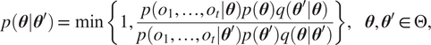 $$ p\left(\boldsymbol{\theta} |{\boldsymbol{\theta}}^{\prime}\right)=\min \left\{1,\frac{p\left({o}_1,\dots, {o}_t|\boldsymbol{\theta} \right)p\left(\boldsymbol{\theta} \right)q\left({\boldsymbol{\theta}}^{\prime }|\boldsymbol{\theta} \right)}{p\left({o}_1,\dots, {o}_t|{\boldsymbol{\theta}}^{\prime}\right)p\left({\boldsymbol{\theta}}^{\prime}\right)q\left(\boldsymbol{\theta} |{\boldsymbol{\theta}}^{\prime}\right)}\right\},\hskip1em \boldsymbol{\theta}, {\boldsymbol{\theta}}^{\prime}\in \Theta, $$
where  $ q\left(\boldsymbol{\theta} |{\boldsymbol{\theta}}^{\prime}\right) $ is any valid MCMC proposal (Andrieu et al., Reference Andrieu, De Freitas, Doucet and Jordan2003). Efficient proposals, such as those by Hamiltonian Monte Carlo (HMC) (Neal, Reference Neal, Brooks, Gelman, Jones and Meng2011), can ensure exploration and decorrelate particles.
4.1.1. The static SMC algorithm
The resulting SMC posterior update algorithm is presented in Algorithm 2. In contrast with Algorithm 1, we accumulate old weights and use them alongside the particles to compute an ESS. As suggested by previous approaches (Del Moral et al., Reference Del Moral, Doucet and Jasra2012), one may keep a good enough posterior approximation by resampling the particles only when their ESS goes below a certain pre-specified thresholdFootnote 2  $ {n}_{\mathrm{min}}\le n $, which reduces computational costs. Whenever this happens, we also move the particles according to the MCMC kernel. This allows us to maintain a diverse particle set, avoiding particle degeneracy. Otherwise, case the ESS is still acceptable, we simply update the particle weights and continue.

4.1.2. Computational complexity
The MCMC-based approach incurs an  $ O(nt) $ computational cost per SMC iteration that grows linearly with the number of particles $ n $ and observations $ t $, instead of remaining constant at $ O(n) $ across iterations as in basic SMC (Algorithm 1). However, this increased computational cost is still relatively low in terms of run-time complexity when compared to the GP modeling approach. Namely, the time complexity for GP updates is $ O\left({t}^3\right) $, which scales cubically with the number of data points (Rasmussen and Williams, Reference Rasmussen and Williams2006). The SMC approach is also low in terms of memory storage costs, as it does not require storing a covariance matrix (quadratic scaling $ O\left({t}^2\right) $) over the data points, but only the points themselves and a set of particles with fixed size, that is, an $ O\left(n+t\right) $ memory cost.
4.2. An UCB algorithm for learning with SMC models
We now define an acquisition function based on an UCB strategy. Compared to the GP-based UCB (Srinivas et al., Reference Szörényi, Busa-Fekete, Weng and Hüllermeier2010), which is defined in terms of posterior mean and variance, SMC provides us with flexible nonparametric distributions which can adjust well to non-Gaussian cases. A natural approach to take advantage of this fact is to the define the UCB in terms of quantile functions (Kaufmann et al., Reference Kaufmann, Cappé and Garivier2012).
The quantile function  $ q $ of a real random variable $ \tilde{s} $ with distribution $ {P}_{\tilde{s}} $ corresponds to the inverse of its cumulative distribution. We define the (upper) quantile function as:
 $$ {q}_{\tilde{s}}\left(\tau \right):= \operatorname{inf}\left\{s\in \unicode{x211D}\hskip0.3em |\hskip0.3em ,{P}_{\tilde{s}}\left(\tilde{s}\le s\right)\ge \tau \right\},\hskip1em \tau \in \left(0,1\right). $$
For probability distributions with compact support, we also define  $ {q}_{\tilde{s}}(0) $ as the minimum and $ {q}_{\tilde{s}}(1) $ as the maximum of $ \tilde{s} $, respectively, of the support of $ {P}_{\tilde{s}} $. In essence, a quantile $ {q}_{\tilde{s}}\left(\tau \right) $ is an upper bound on the value of $ \tilde{s} $ which holds with probability at least $ \tau $.
4.2.1. Empirical quantile functions
In our case, we want to bound  $ f\left(\mathbf{x}\right) $ at any $ \mathbf{x}\in \mathcal{S} $ with high probability. However, we have no direct access to the distribution of $ f\left(\mathbf{x}\right) $. Instead, we use SMC to keep track of its posterior by a set of weighted particles $ {\left\{{\boldsymbol{\theta}}_t^i,{w}_t^i\right\}}_{i=1}^n $ at each iteration $ t $. As $ f\left(\mathbf{x}\right)=h\left(\mathbf{x},\boldsymbol{\theta} \right) $, we have a corresponding empirical approximation to the posterior probability measure of $ f\left(\mathbf{x}\right) $, denoted by $ {\hat{P}}_{f\left(\mathbf{x}\right)}^t:= {\sum}_{i=1}^n{w}_t^i{\delta}_{h\left(\mathbf{x},{\boldsymbol{\theta}}_t^i\right)} $. With the empirical posterior, we approximate the quantile function on $ f\left(\mathbf{x}\right) $ as:
 $$ {q}_{f\left(\mathbf{x}\right)}\left(\tau \right)\approx {\hat{q}}_t\left(\mathbf{x},\tau \right):= \operatorname{inf}\left\{s\in \unicode{x211D}|{\hat{P}}_{f\left(\mathbf{x}\right)}^t\left(f\left(\mathbf{x}\right)\le s\right)\ge \tau \right\},\hskip1em \tau \in \left(0,1\right). $$
In practice, computing  $ {\hat{q}}_t\left(\mathbf{x},\tau \right) $ amounts to sorting realizations of $ f\left(\mathbf{x}\right) $, $ {s}_1\le {s}_2\le \dots \le {s}_n $, according to the empirical posterior $ {s}_i\sim {\hat{P}}_t\left(f\left(\mathbf{x}\right)\right) $ and finding the first element $ {s}_i $ whose cumulative weight $ {\sum}_{j\le i}{w}_j $ is greater than $ \tau $. For $ {\hat{q}}_t\left(\mathbf{x},\tau \right) $ with $ \tau $ set to 0 or 1, the procedure would reduce to returning the supremum or infimum, respectively, in the support of the distribution of $ f\left(\mathbf{x}\right) $, which correspond to $ +\infty $ or $ -\infty $ in the unbounded case.
The quality of empirical quantile approximations for confidence intervals can be quantified via the Dvoretzky–Kiefer–Wolfowitz inequality, which bounds the error on the empirical cumulative distribution function (CDF). Massart, Reference Massart1990 provided a tight bound in that regard.
Lemma 1 (Massart (Reference Massart1990). Let  $ {P}_n:= \frac{1}{n}{\sum}_{i=1}^n{d}_{\xi^i} $ denote the empirical measure derived from $ n\in \unicode{x2115} $ i.i.d. real-valued random variables $ {\left\{{\xi}^i\right\}}_{i=1}^n\overset{\mathrm{i}.\mathrm{i}.\mathrm{d}.}{\sim }P $. For any $ \xi \sim P $, assume the cumulative distribution function $ s\mapsto P\left[\xi \le s\right] $ is continuous, $ s\in \unicode{x211D} $. Then we have that:
 $$ \forall c\in \unicode{x211D},\hskip1em \unicode{x2119}\left\{\underset{s\in \unicode{x211D}}{\sup}\left|{P}_n\left[\xi \le s\right]-P\left[\xi \le s\right]\right|>c\right\}\le 2\exp \left(-2{nc}^2\right). $$
Although SMC samples are inherently biased with respect to the true posterior, we explore methods to transform SMC particles into approximately i.i.d. samples from the true posterior. For instance, the MCMC moves follow the true posterior, which turn the particles into approximate samples of the true posterior. In addition, other methods such as density estimation and the jackknife (Efron, Reference Efron, Kotz and Johnson1992) allow for decorrelation and bias correction. We explore these approaches in Section 5. As a consequence of Lemma 1, we have the following bound on the empirical quantiles.
Theorem 1 (Szörényi et al. (Reference Thrun, Burgard and Fox2015), Proposition 1)). Under the assumptions in Lemma 1, given  $ \mathbf{x}\in \mathcal{X} $ and $ \delta \in \left(0,1\right) $, the following holds for every $ \rho \in \left[0,1\right] $ with probability at least $ 1-\delta $:
 $$ \forall n\ge 1,\hskip1em {\hat{q}}_{\xi}\left(\rho -{c}_n\left(\delta \right)\right)\le {q}_{\xi}\left(\rho \right)\le {\hat{q}}_{\xi}\left(\rho +{c}_n\left(\delta \right)\right), $$
where  $ {c}_n\left(\delta \right):= \sqrt{\frac{1}{2n}\log \frac{\pi^2{n}^2}{3\delta }} $.
Note that Theorem 1 provides a confidence interval around the true quantile based on i.i.d. empirical approximations. In the case of SMC, however, its particles do not follow the i.i.d. assumption. We address this problem in our method, with further approaches for bias reduction presented in Section 5.
4.2.2. Quantile-based UCB
Given the empirical quantile function in Equation (7), we define the following acquisition function:
 $$ a\left(\mathbf{x}|{\mathcal{D}}_t\right):= {\hat{q}}_t\left(\mathbf{x},{\delta}_t\right),\hskip2em t\ge 0, $$
where  $ {\delta}_t\in \left(0,1\right) $ is a parameter which can be adjusted to maintain a high-probability upper confidence bound, as in GP-UCB (Srinivas et al., Reference Szörényi, Busa-Fekete, Weng and Hüllermeier2010). In contrast to a GP-UCB analogy, we are not using a Gaussian approximation based on the posterior mean and variance of the SMC predictions. We are directly using SMC’s nonparametric approximation of the posterior, which can take arbitrary shape.
Theorem 1 allows us to bound the difference between the quantile function and its empirical approximation in the case of  $ n $ i.i.d. samples. Given $ \mathbf{x}\in \mathcal{X} $ and $ \delta \in \left(0,1\right) $, the following holds for every $ \tau \in \left[0,1\right] $ with probability at least $ 1-\delta $:
 $$ \forall n\ge 1,\hskip1em \hat{q}\left(\mathbf{x},\tau -{c}_n\left(\delta \right)\right)\le q\left(\mathbf{x},\tau \right)\le \hat{q}\left(\mathbf{x},\tau +{c}_n\left(\delta \right)\right), $$
where  $ {c}_n\left(\delta \right):= \sqrt{\frac{1}{2n}\log \frac{\pi^2{n}^2}{3\delta }} $. In the non- i.i.d. case, however, the approximation above is no longer valid. We instead replace $ n $ by the ESS $ {n}_{\mathrm{ESS}} $, which is defined as the ratio between the variance of an i.i.d. Monte Carlo estimator and the variance, or mean squared error (Elvira et al., Reference Elvira, Martino and Robert2018), of the SMC estimator (Martino et al., Reference Martino, Elvira and Louzada2017). With $ {n}_{\mathrm{ESS}}^t $ denoting the ESS at iteration $ t $, we set:
 $$ {\delta}_t:= 1-\delta +{c}_{n_{\mathrm{ESS}}^t}\left(\delta \right). $$
 Several approximations for the ESS are available in the SMC literature (Martino et al., Reference Martino, Elvira and Louzada2017; Huggins and Roy, Reference Huggins and Roy2019), which are usually based on the distribution of the weights of the particles. A classical example is  $ {\hat{n}}_{\mathrm{ESS}}:= \frac{{\left({\sum}_{i=1}^n{w}_i\right)}^2}{\sum_{i=1}^n{w}_i^2} $ (Doucet et al., Reference Doucet, Godsill and Andrieu2000; Huggins and Roy, Reference Huggins and Roy2019). In practice, the simple substitution of $ n $ by $ {\hat{n}}_{\mathrm{ESS}} $ defined above can be enough to compensate for the correlation and bias in the SMC samples. In Section 5, we present further approaches to reduce the SMC approximation error with respect to an i.i.d. sample-based estimator.
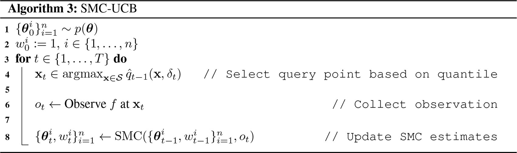
4.2.3. The SMC-UCB algorithm
In summary, the method we propose is described in Algorithm 3, which we refer to as SMC upper confidence bound (SMC-UCB). The algorithm follows the general BO setup with a few exceptions. We start by drawing i.i.d. samples from the model parameters’ prior and equal weights, following the SMC setup (see Algorithm 2). At each iteration  $ t\le T $, we choose a query point by maximizing the acquisition function given by the empirical quantile. We then collect an observation at the selected location. The SMC particles distribution is updated using the new observation, and the algorithm proceeds. As in the usual BO setup, this loop repeats for a given budget of $ T $ evaluations.
5. Drawing Independent Posterior Samples from SMC
Applying to SMC estimates a result similar to Theorem 1 would allow us to provide accurate confidence intervals based on SMC. This result is not directly applicable, however, due to the bias and correlation among SMC samples. Hence we propose an approach to decorrelate samples and remove the bias in SMC estimates.
The approach we propose consists of three main steps. We first decorrelate SMC samples by estimating a continuous density over the SMC particles. The resulting probability distribution is then used as a proposal for importance sampling. The importance sampling estimate provides us with a still biased estimate of expected values under the true posterior. To remove this bias, we finally apply the jackknife method (Efron, Reference Efron, Kotz and Johnson1992).
Throughout this section, our main object of interest will be the expected value of a function of the parameters  $ u:\Theta \to \unicode{x211D} $, which we will assume to be bounded and continuous. We want to minimize the bias in expected value estimates:
 $$ {\varepsilon}_u:= \unicode{x1D53C}\left[u\left(\boldsymbol{\theta} \right)|{\mathcal{D}}_t\right]-\hat{\unicode{x1D53C}}\left[u\left(\boldsymbol{\theta} \right)|{\mathcal{D}}_t\right], $$
where  $ \hat{\unicode{x1D53C}}\left[\cdot \right] $ denotes the SMC-based expected value estimator.
5.1. Density estimation
As a first step, we consider the problem of decorrelating SMC particles by sampling from an estimated continuous probability distribution  $ q $ over the particles. The simplest approach would be to use a Gaussian approximation to the parameters posterior density. In this case, we approximate $ p\left(\boldsymbol{\theta} |{\mathcal{D}}_t\right)\approx {\hat{p}}_t\left(\boldsymbol{\theta} \right):= \mathcal{N}\left(\boldsymbol{\theta}; {\hat{\boldsymbol{\theta}}}_t,{\mathtt{\varSigma}}_t\right) $, where $ \hat{\boldsymbol{\theta}} $ and $ \mathtt{\varSigma} $ correspond to the sample mean and covariance of the SMC particles. However, this approach does not properly capture multimodality and asymmetry in the SMC posterior. In our case, instead, we use a kernel density estimator (Wand and Jones, Reference Wang and Jegelka1994):
 $$ {\hat{p}}_t\left(\boldsymbol{\theta} \right):= \sum \limits_{i=1}^n{w}_t^i{k}_q\left(\boldsymbol{\theta}, {\boldsymbol{\theta}}_t^i\right), $$
with the kernel  $ {k}_q:\Theta \times \Theta \to \unicode{x211D} $ chosen so that the constraint $ {\int}_{\Theta}q\left(\boldsymbol{\theta} \right)\mathrm{d}\boldsymbol{\theta } =1 $ is satisfied. In particular, applying normalized weights, we use a Gaussian kernel for our problems $ {k}_q\left(\boldsymbol{\theta}, {\boldsymbol{\theta}}_t^i\right):= \mathcal{N}\left(\boldsymbol{\theta}; {\boldsymbol{\theta}}_t^i,{\sigma}_q^2\mathbf{I}\right) $, where $ {\sigma}_q>0 $ corresponds to the kernel’s bandwidth. Machine learning methods for density estimation, such as normalizing flows (Dinh et al., Reference Dinh, Sohl-Dickstein and Bengio2017; Kobyzev et al., Reference Kobyzev, Prince and Brubaker2020) and kernel embeddings (Schuster et al., Reference Schuster, Mollenhauer, Klus and Muandet2020), are also available in the literature. However, we do not apply more complex methods to our framework to preserve the simplicity of the approach, also noticing that simple kernel density estimation provided reasonable results in preliminary experiments.
5.2. Importance reweighting
Having a probability density function  $ {\hat{p}}_t $ and a corresponding distribution which we can directly sample from, we draw i.i.d. samples $ {\left\{{\boldsymbol{\theta}}_{{\hat{p}}_t}^i\right\}}_{i=1}^n\overset{\mathrm{i}.\mathrm{i}.\mathrm{d}.}{\sim }{\hat{p}}_t $. The importance sampling estimator of $ \unicode{x1D53C}\left[u\left(\boldsymbol{\theta} \right)|{\mathcal{D}}_t\right] $ using $ {\hat{p}}_t $ as a proposal distribution is given by:
 $$ \mathbf{x}\in \mathcal{X},\hskip1em \unicode{x1D53C}\left[u\left(\boldsymbol{\theta} \right)|{\mathcal{D}}_t\right]=\int u\left(\boldsymbol{\theta} \right)p\left(\boldsymbol{\theta} |{\mathcal{D}}_t\right)\;\mathrm{d}\boldsymbol{\theta } =\int u\left(\boldsymbol{\theta} \right)\frac{p\left(\boldsymbol{\theta} |{\mathcal{D}}_t\right)}{{\hat{p}}_t\left(\boldsymbol{\theta} \right)}{\hat{p}}_t\left(\boldsymbol{\theta} \right)\;\mathrm{d}\boldsymbol{\theta } \approx \sum \limits_{i=1}^nu\left({\boldsymbol{\theta}}_{{\hat{p}}_t}^i\right)\frac{p\left({\boldsymbol{\theta}}_{{\hat{p}}_t}^i|{\mathcal{D}}_t\right)}{{\hat{p}}_t\left({\boldsymbol{\theta}}_{{\hat{p}}_t}^i\right)}. $$
We, however, do not have access to  $ p\left({\mathcal{D}}_t\right) $ to compute $ p\left(\boldsymbol{\theta} |{\mathcal{D}}_t\right) $. Therefore, we do another approximation using the same proposal samples:
 $$ p\left({\mathcal{D}}_t\right)={\int}_{\Theta}p\left({\mathcal{D}}_t|\boldsymbol{\theta} \right)p\left(\boldsymbol{\theta} \right)\;\mathrm{d}\boldsymbol{\theta } ={\int}_{\Theta}p\left({\mathcal{D}}_t|\boldsymbol{\theta} \right)\frac{p\left(\boldsymbol{\theta} \right)}{{\hat{p}}_t\left(\boldsymbol{\theta} \right)}{\hat{p}}_t\left(\boldsymbol{\theta} \right)\;\mathrm{d}\boldsymbol{\theta } \approx \sum \limits_{i=1}^np\left({\mathcal{D}}_t|{\boldsymbol{\theta}}_{{\hat{p}}_t}^i\right)\frac{p\left({\boldsymbol{\theta}}_{{\hat{p}}_t}^i\right)}{{\hat{p}}_t\left({\boldsymbol{\theta}}_{{\hat{p}}_t}^i\right)}. $$
Setting  $ {\alpha}_t^i:= p\left({\mathcal{D}}_t|{\boldsymbol{\theta}}_{{\hat{p}}_t}^i\right)\frac{p\left({\boldsymbol{\theta}}_{{\hat{p}}_t}^i\right)}{{\hat{p}}_t\left({\boldsymbol{\theta}}_{{\hat{p}}_t}^i\right)} $, we then have:
 $$ \unicode{x1D53C}\left[u\left(\boldsymbol{\theta} \right)|{\mathcal{D}}_t\right]\approx \frac{1}{\eta_t}\sum \limits_{i=1}^n{\alpha}_t^iu\left({\boldsymbol{\theta}}_{{\hat{p}}_t}^i\right),\hskip1em \mathbf{x}\in \mathcal{X}, $$
where  $ {\eta}_t:= {\sum}_{i=1}^n{\alpha}_t^i\approx p\left({\mathcal{D}}_t\right) $. This approach has been recently applied to estimate intractable marginal likelihoods of probabilistic models (Tran et al., Reference Urteaga and Wiggins2021).
5.3. Debiasing via the jackknife
There are different sources of bias in the SMC estimate and in the further steps described above. The jackknife method provides sample-based estimates for statistics of a random variable. The method is based on averaging leave-one-out estimates (Efron, Reference Efron, Kotz and Johnson1992). For the case of bias in estimation, consider a set of samples  $ {\left\{{\boldsymbol{\theta}}_i\right\}}_{i=1}^n $ and a function $ u:\Theta \to \unicode{x211D} $. Let $ \hat{u} $ denote the importance-sampling estimate of the expected value of $ u $ according to Equation (16). If we remove a sample $ i\in \left\{1,\dots, n\right\} $, we can reestimate a proposal density and the importance-weighted expected value of $ u $ as $ {\hat{u}}_i $. The jackknife estimate for the bias in the approximation of $ \unicode{x1D53C}\left[u\right] $ is then given by:
 $$ {\hat{u}}_{\mathrm{bias}}:= \left(n-1\right)\left(\frac{1}{n}\sum \limits_{i=1}^n{\hat{u}}_i-\hat{u}\right). $$
Having an estimate for the bias, we can subtract it from the approximation in Equation (16) to compensate for its bias. We compare the effect of this combined with the previous approaches in preliminary experiments presented next.
5.4. Preliminary experiments on bias correction
We ran preliminary experiments to test the effects of debiasing and decorrelation methods for the estimation of the posterior CDF with SMC. Experiments were run with randomized settings, having parameters for the true model sampled from the prior used by SMC. The test model consists of an exponential-gamma model over  $ \Theta \subset \unicode{x211D} $ with a gamma prior $ \theta \sim \Gamma \left(\alpha, \beta \right) $ and an exponential likelihood $ p\left(o|\theta \right)=\theta \exp \left(-\theta o\right) $. Given $ T $ observations, to compute the approximation error, the true posterior is available in closed-form as:
 $$ p\left(\theta |{o}_1,\dots, {o}_T\right)=\Gamma \left(\theta; \alpha +T,\beta +T{\overline{o}}_T\right), $$
where  $ {\overline{o}}_T:= \left(1/T\right){\sum}_{i=1}^T{o}_T $. For this experiment, we set $ \alpha =\beta =1 $ as the prior parameters.
Within each trial, we sampled a parameter  $ \theta $ from the prior to serve as the true model, and generated observations from it. We ran Algorithm 2 with an MCMC kernel equipped with a random walk proposal $ q\left({\theta}^{\prime }|\theta \right):= \mathcal{N}\left({\theta}^{\prime };\theta, {\sigma}^2\right) $ with $ \sigma := 0.1 $. We applied Gaussian kernel density estimation to estimate the parameters’ posterior density, setting the median distance between particles as the kernel bandwidth.
CDF approximation results are presented in Figures 1 and 2 for the posteriors after  $ T=2 $ and $ T=5 $ observations, respectively. As seen the effects of bias correction methods becomes more evident for SMC posteriors after a larger number of observations is collected. In particular, we highlight the difference between importance reweighting and jackknife results, which is more noticeable for $ T=5 $. The main drawback of the jackknife approach, however, is its increased computational cost due to the repeated leave-one-out estimates. In our main experiments, therefore, we present the effects of the importance reweighting correction compared to the standard SMC predictions.
Posterior CDF approximation errors for the exponential-gamma model using  $ T=2 $ observations. For each sample size, which corresponds to the number of SMC particles, SMC runs were repeated 400 times for each method, except for the jackknife, which was rerun 40 times due to a longer run time.The theoretical upper confidence bound on the CDF approximation error cn(δ) (Theorem 1) is shown as the plotted blue line. The frequency of violation of the theoretical bounds for i.i.d. empirical CDF errors is also presented on the top of each plot, alongside the target ( $ \delta =0.1 $).

Posterior CDF approximation errors for the exponential-gamma model using  $ T=5 $ observations. For each sample size, which corresponds to the number of SMC particles, SMC runs were repeated 400 times for each method, except for the jackknife, which was rerun 40 times due to a longer run time.The theoretical upper confidence bound on the CDF approximation error cn(δ) (Theorem 1) is shown as the plotted blue line. The frequency of violation of the theoretical bounds for i.i.d. empirical CDF errors is also presented on the top of each plot, alongside the target ( $ \delta =0.1 $).

5.5. Limitations
As a few remarks on the limitations of the proposed framework, we highlight that the use of more complex forward models and bias correction methods for the predictions comes at an increased cost in terms of runtime, when compared to simpler models, such as GPs. In practice, one should consider applications where the cost of observations is much larger than the cost of evaluating model predictions. For example, in mineral exploration, collecting observations may involve expensive drilling operations which take a much higher cost than running simulations for a few minutes, or even days, to obtain an SMC estimate. This runtime cost, however, becomes amortized as the number of observations grows, since the computational complexity for GP updates is still  $ O\left({t}^3\right) $, which grows cubically with the number of observations, when compared to an $ O(nt) $ for SMC. Even when considering importance reweighting or optionally combining it with the jackknife method for bias correction, the computational complexity for SMC updates is only added by $ O(nt) $ or $ O\left({n}^2t\right) $, respectively, which are both linear with respect to the number of observations. Lastly, the compromise between accuracy and speed can be controlled by adjusting the number of particles $ n $ used by the algorithm. As each particle corresponds to an independent simulation by the forward model, these simulations can also be executed simultaneously in parallel, further reducing the algorithm’s runtime. The following section presents experimental results on practical applications involving water resources monitoring, which in practice present a suitable use case for our framework, given the cost of observations and the availability of informative physics simulation models.
6. Experiments
In this section, we present experimental results comparing SMC-UCB against its GP-based counterpart GP-UCB (Srinivas et al., Reference Szörényi, Busa-Fekete, Weng and Hüllermeier2010) and the GP expected improvement (GP-EI) algorithm (Jones et al., Reference Jones, Schonlau and Welch1998), which does not depend on a confidence parameter. We assess the effects of the SMC approximation and its optimization performance in different problem settings. As a performance metric, we use the algorithm’s regret  $ {r}_t:= {\max}_{\mathbf{x}\in \mathcal{S}}f\left(\mathbf{x}\right)-f\left({\mathbf{x}}_t\right) $. The averaged regret provides an upper bound on the minimum regret of the algorithm up to iteration $ T $, that is, $ {\min}_{t\le T}{r}_t\le \frac{1}{T}{\sum}_{t=1}^T{r}_t $. A vanishing average regret (as $ T\to \infty $) indicates that the choices of the algorithm get arbitrarily close to the optimal solution $ {\mathbf{x}}^{\ast } $ in Equation (1).
6.1. Linear Gaussian case
Our first experiment is set with a linear Gaussian model, where the true posterior over the parameters is available in closed form and corresponds to a degenerate (i.e., finite-dimensional) GP. As a synthetic data example, we sample true parameters from their prior distribution  $ \theta \sim \mathcal{N}\left(\mathbf{0},\mathbf{I}\right) $ and set $ f\left(\mathbf{x}\right):= {\theta}^{\mathrm{T}}\phi \left(\mathbf{x}\right) $, where $ \phi :\mathcal{X}\to {\unicode{x211D}}^m $ is a kernel-based feature map $ \phi \left(\mathbf{x}\right)={\left[k\left(\mathbf{x},{\mathbf{x}}_1\right),\dots, k\left(\mathbf{x},{\mathbf{x}}_m\right)\right]}^{\mathrm{T}} $ with $ {\left\{{\mathbf{x}}_i\right\}}_{i=1}^m\sim \mathcal{U}\left(\mathcal{S}\right) $, and $ \mathcal{S}:= {\left[0,1\right]}^d $, $ d:= 2 $. We set $ k $ as a squared-exponential kernel (Rasmussen and Williams, Reference Rasmussen and Williams2006) with length-scale $ \mathrm{\ell}:= 0.2 $. The parameters prior $ \theta \sim \mathcal{N}\left(\mathbf{0},\mathbf{I}\right) $ and the likelihood $ o\mid f\left(\mathbf{x}\right)\sim \mathcal{N}\left(f\left(\mathbf{x}\right),{\sigma}_{\varepsilon}^2\right) $ are both Gaussian, with $ {\sigma}_{\varepsilon }=0.1 $. In this case, the posterior given $ t $ observations $ {\mathcal{D}}_t={\left\{{\mathbf{x}}_t,{o}_t\right\}}_{i=1}^t $ is available in closed form as:
 $$ \boldsymbol{\theta} \mid {\mathcal{D}}_t\sim \mathcal{N}\left({\mathbf{A}}_t^{-1}\mathtt{\varPhi}{\mathbf{o}}_t,{\sigma}_{\varepsilon}^2{\mathbf{A}}_t^{-1}\right), $$
where  $ {\mathbf{A}}_t:= {\mathtt{\varPhi}}_t{\mathtt{\varPhi}}_t^{\mathrm{T}}+{\sigma}_{\varepsilon}^2\mathbf{I} $, $ {\mathtt{\varPhi}}_t:= \left[\phi \left({\mathbf{x}}_1\right),\dots, \phi \left({\mathbf{x}}_t\right)\right] $ and $ {\mathbf{o}}_t:= {\left[{o}_1,\dots, {o}_t\right]}^{\mathrm{T}} $.
As a move proposal for SMC, we use a Gaussian random walk (Andrieu et al., Reference Andrieu, De Freitas, Doucet and Jordan2003) within a Metropolis-Hastings kernel. We use the same standard normal prior for the parameters and the linear Gaussian likelihood based on the same feature map. For all experiments, we set  $ \delta := 0.3 $ for SMC-UCB.
We first compared SMC-UCB against GP-UCB in the optimization setting with different settings for the number of particles  $ n $. GP-UCB (Srinivas et al., Reference Szörényi, Busa-Fekete, Weng and Hüllermeier2010) followed Durand et al. (Reference Durand, Maillard and Pineau2018, Theorem 2) for the setting of the UCB parameter, and the GP covariance function was set as the same kernel in the feature map. We also set $ \delta := 0.3 $ for GP-UCB. The resulting regret across iterations is shown in Figure 3a. We observe that SMC-UCB is able to attain faster convergence rates than GP-UCB for $ n\ge 300 $ particles. A factor driving this improvement is that the quantile approximation error quickly decreases with $ n $, as seen in Figure 3b.
Linear Gaussian case: (a) mean regret of SMC-UCB for different  $ n $ compared to the GP-UCB baseline with parameter dimension $ m:= 10 $; (b) approximation error between the SMC quantile $ {\hat{q}}_t\left({\mathbf{x}}_t,{\delta}_t\right) $ and the true $ {q}_t\left({\mathbf{x}}_t,{\delta}_t\right) $ at SMC-UCB’s selected query point $ {\mathbf{x}}_t $ for different $ n $ settings (absent values correspond to cases where $ {\hat{q}}_t\left(\mathbf{x},{\delta}_t\right)=\infty $); (c) comparison with the non-UCB, GP-based expected improvement algorithm; and (d) effect of parameter dimension $ m $ on optimization performance when compared to the median performance of the GP optimization baselines. All results were averaged over 10 runs. The shaded areas correspond to $ \pm 1 $ standard deviation.

Another set of tests compared SMC-UCB using 400 particles and the importance reweighting method in Section 5.5 against GP-UCB and GP-EI. The optimization performance results are presented in Figure 3c and show that SMC-UCB is able to maintain a clear advantage against both GP-based approaches and improve over its no-importance-correction baseline (Figure 3a). In particular, we notice that GP-EI is outperformed by both UCB methods. Lastly, a main concern regarding SMC methods is the decrease in posterior approximation performance as the dimensionality of the parameter space increases. Figure 3d, however, shows that SMC-UCB is able to maintain reasonable optimization performance up to dimensionality  $ m=60 $ when compared to baselines. Although this experiment involved a linear model, we conjecture that similar effects in terms of optimization performance should be observed in models which are at least approximately linear, such as when $ h\left(\mathbf{x},\boldsymbol{\theta} \right) $ is Lipschitz continuous w.r.t. $ \boldsymbol{\theta} $. Yet, a formal theoretical performance analysis is left for future work.
6.2. Water leak detection
As an example of a realistic application scenario, we present an approach to localize leaks in water pipes via SMC and BO. A long rectilinear underground pipe presents a 5-day water leak at an unknown location within a porous soil medium. We have access to a mobile gravimetric sensor on the surface with a very low noise level  $ {\sigma}_{\varepsilon}:= 5\times {10}^{-8} $ m s−2 for gravitational acceleration. The wet soil mass presents higher density than the dry soil in its surroundings, leading to a localized maximum on the gravitational readings. We assume that prior information on gravitational measurements in the area allows us to cancel out the gravity from the surrounding buildings and other underground structures. We performed computational fluid dynamics (CFD) simulationsFootnote 3 to provide “ground-truth” gravity readings $ \mathbf{g}\left(\mathbf{x}\right)={\left[{g}_1\left(\mathbf{x}\right),{g}_2\left(\mathbf{x}\right),{g}_3\left(\mathbf{x}\right)\right]}^{\mathrm{T}} $ at the surface, and took the vertical gravity component $ {g}_3\left(\mathbf{x}\right) $ as our objective function for BO. Figure 5a shows the relative gravity measurements. The true pipe is 2 m in diameter and buried 3 m underground, quantities which are not revealed to BO.
6.2.1. Pipe leak simulation
To provide an objective function consisting of realistic gravity measurements, we simulated a 3D model in the COMSOL Multiphysics software environmentFootnote 4 using some basic assumptions related to soil properties. This tool is a finite-element analysis and simulation software for solving and post-processing computational models of physical systems. For our simulations, in particular, we used the subsurface flow module,Footnote 5 which allows simulating fluid flows in porous media. In detail, the soil porosity is set to 0.339, residual saturation to  $ 1\times {10}^{-3} $, soil storage coefficient to $ 3.4466\times {10}^{-5}\;{\mathrm{Pa}}^{-1} $, saturated hydraulic conductivity to $ 5.2546\times {10}^{-6}\;\mathrm{m}\;{\mathrm{s}}^{-1} $ and the leak from the pipe to 10 kg m−2s−1. For the experiments we use the gravity measured on the surface after 5 days of leakage. Figure 4 shows the spatial arrangement of the simulation. To provide observations to the optimization algorithms, gravity data is corrupted with simulated noise following a quantum gravimeter noise characteristics (Hardman et al., Reference Hardman, Everitt, McDonald, Manju, Wigley, Sooriyabandara, Kuhn, Debs, Close and Robins2016). The resulting data is shown in Figure 5a.
Pipe simulation diagram: A water pipe of 2 in diameter is buried 3 underground in a large block of soil ( $ 100\times 100\times 50\;\mathrm{m} $).
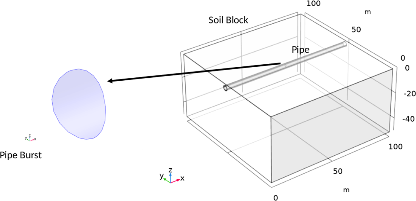
Performance results for water leak detection experiment: (a) The gravity objective function generated by CFD simulations and the mean regret curves for each algorithm. The shaded areas in the plot correspond  $ \pm 1 $ standard deviation results from results which were averaged over 10 trials. (b) The gravity estimates according to the final SMC and GP posteriors after 100 iterations. (c) SMC estimates for the parameters concerning the location of the leak. The upper plot in (c) is colored according to an estimate for the mass of leaked water.
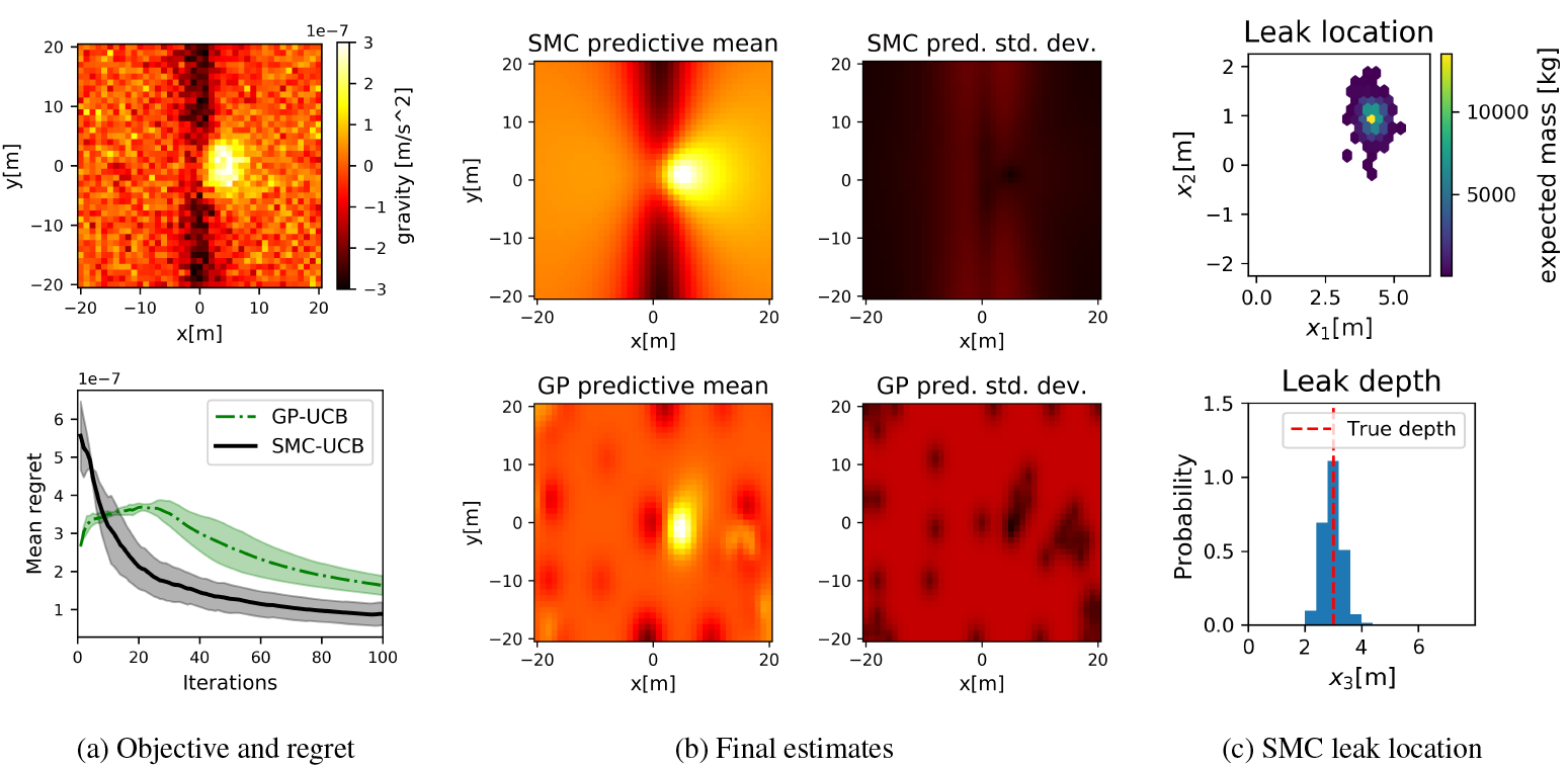
6.2.2. Gravity forward model
To derive an informative model from domain knowledge for SMC, we model the pipe as an infinite cylinder and the leak as a spherical mass, which have closed-form expressions for their gravitational field (Young and Freedman, Reference Young and Freedman2015). The gravity of an infinite cylinder of density  $ {\rho}_P $ and radius $ {r}_P $ passing by a location $ {\mathbf{x}}_P $ at a given direction $ {\mathbf{u}}_P\in {\unicode{x211D}}^3 $ can be derived as:
 $$ {\mathbf{g}}_P\left(\mathbf{x}\right)=-\frac{2G{\pi \rho}_P{r}_P^2{\mathbf{u}}_P\times \left(\mathbf{x}-{\mathbf{x}}_P\right)\times {\mathbf{u}}_P}{\parallel \left(\mathbf{x}-{\mathbf{x}}_P\right)\times {\mathbf{u}}_P{\parallel}_2^2}, $$
where  $ G:= 6.674\times {10}^{-11}\;{\mathrm{m}}^3{\mathrm{kg}}^{-1}{\mathrm{s}}^{-2} $ represents Newton’s gravitation constant. For the leak, the gravity of a uniform sphere of density $ {\rho}_S $ and radius $ {r}_S $ centerd at location $ {\mathbf{x}}_S\in {\unicode{x211D}}^3 $ is given by:
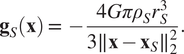 $$ {\mathbf{g}}_S\left(\mathbf{x}\right)=-\frac{4G{\pi \rho}_S{r}_S^3}{3\parallel \mathbf{x}-{\mathbf{x}}_S{\parallel}_2^2}. $$
6.2.3. Likelihood
As an observation model, we use Equations (20) and (21) to compose a Gaussian likelihood model based on the gravity of the pipe  $ {\mathbf{g}}_P $ and of the wet-soil sphere $ {\mathbf{g}}_S $. As gravity is an integral over distributions of mass, Gaussian noise is a well-suited assumption due to the central limit theorem (Bauer, Reference Bauer1981). So we set $ p\left({o}_t|\boldsymbol{\theta}, \mathbf{x}\right)=\mathcal{N}\left({o}_t;{g}_{P,3}\left(\mathbf{x}\right)+{g}_{S,3}\left(\mathbf{x}\right),{\sigma}_{\varepsilon}^2\right) $ for the gravity model parameters $ \boldsymbol{\theta} := {\left[{\mathbf{x}}_P^{\mathrm{T}},{r}_P,{\rho}_P,{\mathbf{u}}_P^{\mathrm{T}},{\mathbf{x}}_S^{\mathrm{T}},{r}_S,{\rho}_S\right]}^{\mathrm{T}} $ based on the vertical-axis gravity measurements with $ {\sigma}_{\varepsilon}:= 5\times {10}^{-8} $ m s−2, the noise level of the gravity sensor we consider (Hardman et al., Reference Hardman, Everitt, McDonald, Manju, Wigley, Sooriyabandara, Kuhn, Debs, Close and Robins2016).
6.2.4. Priors on the pipe
We assume uncertainty on the pipe’s location  $ {\mathbf{x}}_P:= {\left[{x}_{P,1},{x}_{P,2},{x}_{P,3}\right]}^{\mathrm{T}} $, though not on its orientation $ {\mathbf{u}}_P $.Footnote 6 We place a Gaussian prior on the pipe’s horizontal coordinate with $ {x}_{P,1}\sim \mathcal{N}\left(0,1\right) $ and a gamma prior $ \Gamma \left({\alpha}_z,{\beta}_z\right) $ with $ \alpha =2 $ and $ \beta =1 $ on the pipe’s depth, that is, $ -{x}_{P,3} $. For the radius, we set $ {r}_P\sim \Gamma \left({\alpha}_r,{\beta}_r\right) $ with $ {\alpha}_r=2.25 $ and $ {\beta}_r=0.75 $, yielding a 95% confidence interval of $ {r}_P\in \left[\mathrm{0.4,8}\right] $ m. The pipe’s density is set as tightly around the water density $ {\rho}_P\sim \mathcal{N}\left({\hat{\rho}}_P,{\sigma}_{\rho_P}^2\right) $ with $ {\hat{\rho}}_P:= 1000 $ kg m−3 and $ {\sigma}_{\rho_P}:= 10 $ kg m−3, which allows for small variations in the pipe’s mass distribution due to the outflow of water with the leak.
6.2.5. Priors on the sphere
For the wet soil sphere, we place conditional priors  $ {x}_{S,1}\mid {x}_{P,1},{r}_P\sim \mathcal{N}\left({x}_{P,1},{r}_P^2/4\right) $ and $ \left({x}_{P,3}-{x}_{S,3}\right)/{x}_{P,3}\sim \mathrm{Beta}\left(2,5\right) $, indicating that the leak is most likely concentrated somewhere around the pipe’s border. However, the leak’s $ {x}_{S,2} $ coordinate, which goes along the pipe, is only known to be within a bounded segment of the pipe, $ {x}_{S,2}\sim \mathcal{U}\left(-20,20\right) $. As a leak is a rare phenomenon, we place priors with high probability around zero for the leak’s radius and density. In particular, we set a 1-degree-of-freedom chi-square distribution for $ {r}_S\sim {\chi}^2(1) $, and the density as a gamma random variable $ {\rho}_S\sim \Gamma ({\alpha}_{\rho },{\beta}_{\rho }) $ with $ {\alpha}_{\rho }=2 $ and $ {\beta}_{\rho }=1/250 $, so that $ {\rho}_S\in \left[100,1000\right] $ kg with approximately 90% probability.
6.2.6. SMC settings
A HMC kernel within SMC was configured with 100 leapfrog steps and per-parameter tuned step sizes, according to their prior distribution.Footnote 7 The number of particles is set to  $ n:= 1000 $.
6.2.7. Optimization settings
GP-UCB and SMC-UCB were run with similar settings. GP hyperparameters were learnt offline via maximum a posteriori estimation. The GP covariance function was a Matérn function with smoothness parameter  $ \nu := 2.5 $ (see Rasmussen and Williams, Reference Rasmussen and Williams2006, Ch. 4) SMC-UCB was configured with $ \delta := 0.1 $. As we do not have enough information about the objective function to derive theory-recommended UCB parameters, GP-UCB was set with an equivalent UCB parameter based on the inverse CDF of a normal distribution. For both methods, the acquisition function optimization is performed over a discretized fine grid covering the search space.
6.2.8. Results
Figure 5 presents results for the leak detection experiment. As the plot in Figure 5a shows, the proposed SMC-UCB algorithm is able to overcome GP-UCB in this setting with a clearly lower regret from the beginning. The SMC method also presents final predictions better approximating the provided CFD data with low uncertainty on the sphere position parameters, as seen in Figure 5b. Due to exploration–exploitation trade-off of BO algorithms (Brochu et al., Reference Brochu, Cora and de Freitas2010; Shahriari et al., Reference Shahriari, Swersky, Wang, Adams and De Freitas2016), it is natural that the uncertainty regarding the pipe’s parameters is slightly higher, as its gravity does not directly contribute to the maximum of the gravity objective function. Yet we can see that SMC’s estimate on the pipe’s gravity signature is still evident when compared to the GP’s estimated gravity predictions (see Figure 5c). In addition, SMC is able to directly estimate the leak’s location online based on its empirical posterior parameters distribution. With GPs the same would require running a second inference scheme using all the observations.
6.3. Contaminant source localization
As a final experiment to demonstrate the potential of SMC for BO, we present the problem of localizing a source of contamination within an aquifer with strong property contrasts (Pirot et al., Reference Pirot, Krityakierne, Ginsbourger and Renard2019). We transform the source localization problem into that of finding the maximum contaminant concentration over a set of 25 possible well locations. We have access to hydraulic simulationsFootnote 8 (Cornaton, Reference Cornaton2007) made available by Pirot et al. (Reference Pirot, Krityakierne, Ginsbourger and Renard2019) predicting the contaminant concentration at  $ \mathcal{S}={\left\{{\mathbf{x}}_i\right\}}_{i=1}^L $, where $ L:= 25 $ possible well locations over a window of 300 days with candidate contaminant source locations $ \boldsymbol{\theta} := {\mathbf{x}}_C $ spread over a 51-by-51, 3-meter cell grid, totalling 2,601 possible locations.
6.3.1. Data
The contaminant concentration data is composed of two datasets, one with the simulated concentration values for all 25 wells and all 301 measurement times over the 51-by-51 source locations grid, while the other dataset consists of reference “real” concentration values over the 25 wells and the 301 time steps. The “real” concentration values are in fact simulated concentration values at locations not revealed to the BO algorithms. To simulate different scenarios, each experiment trial was run on a random day, sampled uniformly among the 300 days. To provide observations for each algorithm, we also add Gaussian noise with  $ {\sigma}_{\varepsilon}:= 1\times {10}^{-3} $, corresponding to roughly a 10% measurement error level.
6.3.2. SMC model
We use the hydraulic simulations to form a model for SMC-UCB using  $ n:= 400 $ particles. A separate dataset of simulated concentrations is used as the objective function. SMC is configured with a Metropolis-Hastings move kernel using a proposal over the discrete source locations space. At each move, we compute the current posterior probabilities at each point in the location space and form an empirical distribution with it, which is our proposal distribution.
6.3.3. Optimization settings
For this experiment, we set SMC-UCB with  $ \delta := 0.3 $. GP-UCB is set with a fixed value for the UCB parameter $ {\beta}_t:= 3 $, which was the best performing for this experiment after tuning with preliminary runs. To provide a tuned GP model, we compute an empirical covariance matrix for the well measurements data from a random subset of the 2,601 possible source locations. With this empirical covariance matrix, we form a zero-mean GP over the discrete search space. This procedure is similar to common practice in the GP-UCB literature when real datasets are provided (Srinivas et al., Reference Szörényi, Busa-Fekete, Weng and Hüllermeier2010; Chowdhury and Gopalan, Reference Chowdhury and Gopalan2017).
6.3.4. Results
Figure 6 presents our experimental results for the contaminant source localization problem. As Figure 6a shows, SMC-UCB is able to achieve a better performance than GP-UCB by using the informative prior coming from hydraulic simulations. In addition, SMC final parameter estimates (Figure 6b) present high probability mass around the true source location.
Contaminant source localization problem: (a) The optimization performance of each algorithm in terms of regret. Results were averaged over 10 runs. (b) A final SMC estimate for the source location, while the true location is marked as a red star.
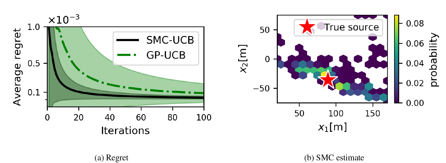
7. Conclusion
This article presented SMC as an alternative to GP based approaches for Bayesian optimization when domain knowledge is available in the form of informative computational models. We presented a quantile-based acquisition function for BO which is adjusted for the effects of the approximation bias in the SMC estimates and allows for inference based on non-Gaussian posterior distributions. The resulting SMC algorithm is shown to outperform the corresponding GP-based baseline in different problem scenarios.
The work in this article can be seen as a starting point toward a wider adoption of SMC algorithms in BO applications. Further studies with theoretical assessments of the SMC approximation should strengthen the approach and allow for the derivation of new algorithms which can make an impact on the practical use of BO in data-driven science and engineering applications. Another interesting direction of future research is the incorporation of likelihood-free SMC (Sisson et al., Reference Sisson, Fan and Tanaka2007) methods into the BO loop in cases where forward models do not allow for a closed-form expression of the observation model.
Data Availability Statement
The data for the contaminant source localization experiment is available at https://github.com/gpirot/BGICLP.
Author Contributions
Conceptualization: R.O., R.S., R.K., S.C., J.C.; Data curation: K.H., N.T.; Formal analysis: R.O.; Funding acquisition: R.S., R.K., S.C., J.C., C.L; Investigation: R.O., K.H., N.T., C.L; Methodology: R.O., R.K.; Software: R.O.; Supervision: R.S., R.K., S.C., C.L.; Writing—original draft: R.O. All authors approved the final submitted draft.
Funding Statement
Parts of this research were conducted by the Australian Research Council Industrial Transformation Training Centre in Data Analytics for Resources and the Environment (DARE), through project number IC190100031.
Acknowledgment
Rafael Oliveira was supported by the Medical Research Future Fund Applied Artificial Intelligence in Health Care grant (MRFAI000097).
Competing Interests
The authors declare no competing interests exist.


 Open access
Comments
No Comments have been published for this article.