


Impact statement
Lack of adequate acknowledgment of shortcomings of bottom-up load forecasting approaches has led to methodologies that are not practical on a large scale or contribute to myopic results about the advantages of fine-resolution smart-meter data. The implications of such misleading results can range from discouraging practitioners from seeking the tremendous value of big smart-meter data to picking a prediction model that is not compatible with fine-resolution big data and leads to sub-optimal predictions. The insights from this study are, therefore, of critical importance for policy-makers and infrastructure managers, especially in light of the government’s record investments in big data and artificial intelligence (AI) technology and the ambitious decarbonization targets that warrant access to scalable and accurate energy forecasting and management systems.
1. Introduction
Short-term load forecasting is essential for optimal power system operation and ensuring consumers’ sustained access to electricity (Chen et al., Reference Chen, Chen, Wang, He, Hu and He2018; Fallah et al., Reference Fallah, Ganjkhani, Shamshirband and Chau2019; Liang et al., Reference Liang, Niu and Hong2019; Lin et al., Reference Lin, Wu and Boulet2021; Rafi et al., Reference Rafi, Nahid-Al-Masood, Deeba and Hossain2021). Electricity supply and demand have to be matched in real-time, and since energy storage is still costly (Schmidt et al., Reference Schmidt, Hawkes, Gambhir and Staffell2017; Cole et al., Reference Cole, Frazier and Augustine2021), electric utilities must carefully plan their dispatch to minimize energy loss. Under the traditional paradigm of centralized power generation, utilities rely on predicting a group of building loads rather than building-level loads. As a result, several studies in the literature have attempted to predict the total demand for a large group of buildings (Eskandari et al., Reference Eskandari, Imani and Moghaddam2021; Hu et al., Reference Hu, Qu, Wang, Liang, Wang, Yu, Li and Qiao2021; Massaoudi et al., Reference Massaoudi, Refaat, Chihi, Trabelsi, Oueslati and Abu-Rub2021; Yin and Xie, Reference Yin and Xie2021). In most cases, these studies take a top-down approach, predicting demand at an aggregated level based on previously observed aggregated data demand. In other words, fine-resolution data from smart meters are not included in such prediction models.
More recently, due to the increasing need for distributed supply–demand management and the rising availability of smart-meter data, grid operators and researchers are seeking to advance accurate load forecasting analytics (Chou and Tran, Reference Chou and Tran2018; Zhang et al., Reference Zhang, Grolinger, Capretz and Seewald2018). Specifically, the carbon-neutral energy sector is highly dependent on distributed renewable energy sources, including power generated by grid-interactive buildings. The grid-interactive buildings are designed not only to contribute to clean energy generation but also to maximize energy efficiency by being smarter about the amount and timing of energy usage and providing demand flexibility (Neukomm et al., Reference Neukomm, Nubbe and Fares2019). Such smart demand management requires smart technologies, such as smart meters, for inexpensive communications. Additionally, efficient demand management requires reliable demand prediction, which can be facilitated via fine-resolution smart-meter data. This has prompted researchers to exploit fine-resolution data for predicting demand at both building- and utility-level.
Demand prediction at the utility level using smart-meter data is primarily achieved through a bottom-up approach, which involves grouping smart-meter data into clusters and developing independent prediction models for each cluster. The predicted demands across all clusters are subsequently aggregated to estimate the total demand (Alzate and Sinn, Reference Alzate and Sinn2013; Quilumba et al., Reference Quilumba, Lee, Huang, Wang and Szabados2014; Shahzadeh et al., Reference Shahzadeh, Khosravi and Nahavandi2015; Wijaya et al., Reference Wijaya, Vasirani, Humeau and Aberer2015; Wang et al., Reference Wang, Lee, Huang, Szabados, Wang and Van Olinda2016; Fahiman et al., Reference Fahiman, Erfani, Rajasegarar, Palaniswami and Leckie2017; Fu et al., Reference Fu, Zeng, Feng and Cai2018; Bian et al., Reference Bian, Zhong, Sun and Shi2020). While such a bottom-up approach is conducive to exploiting high-resolution smart-meter data, its applicability has only been demonstrated on test sets with at most a few thousand customers. In this paper, we discuss the scalability issue of the bottom-up approach and explain why it is not applicable when smart-meter data from millions of customers is available. In fact, a bottom-up approach in such scenarios can easily result in sub-optimal predictions, which can be hugely costly. To provide an idea about the imposed cost, one should note that a 1% reduction in forecasting error for a utility company can save up to between $300 thousand to $1.6 million annually (Hobbs et al., Reference Hobbs, Jitprapaikulsarn, Konda, Chankong, Loparo and Maratukulam1999; Hong, Reference Hong2015). Notably, this does not include additional social or environmental costs arising from wasting energy or blackouts caused by inaccurate load forecasts.
At the building level, with multiple independent apartment units, the advent of smart-meter technology has made it possible to obtain even one-minute energy consumption data for each unit. In order to facilitate efficient deployment and installation of advanced smart-metering devices, a seminal paper by Jain et al. (Reference Jain, Smith, Culligan and Taylor2014) studied the scales at which data can be distilled into meaningful information. To this end, they made the first effort to evaluate the impact of temporal and spatial data granularity on forecasting accuracy. Specifically, to compare the accuracy offered by different data granularity, they developed forecast models at different spatial and temporal resolutions and used the bottom-up approach to predict overall consumption for the whole building.
By comparing the accuracy of their predictions of total consumption, Jain et al. (Reference Jain, Smith, Culligan and Taylor2014) conclude that the most reliable forecasting can be obtained by using hourly consumption data at the floor level. Specifically, their results show that fine-resolution data (e.g., 10-min consumption at the unit or floor level) decreases the accuracy of prediction. This, however, is counter-intuitive as the information in coarse-resolution data is embedded in fine-resolution data. For instance, if unit-level data is available, floor-level data can be calculated through a simple arithmetic sum. This begs the question of how it might be possible to yield less accurate forecasts with data at the unit level compared to the floor level. In this paper, we will discuss how this seemingly counter-intuitive result stems from one of the most prevalent shortcomings of the bottom-up approach, namely error aggregation. We show that error aggregation in building-level load forecasts can result in sub-optimal predictions. In a distributed energy grid that is highly dependent on renewable energy sources and load management, such sub-optimal predictions can substantially reduce the efficiency of load management and result in costly supply shortages or waste of resources.
In what follows, we illustrate and discuss the limitations of the bottom-up approach. To this end, we show results from two experiments. One experiment focuses on predicting the aggregate demand at the utility level using big smart-meter data from 3.7 million customer units. The second experiment concerns predicting building-level demand using data from 21 residential units. Through these two experiments, we shed light on how the blind application of the bottom-up approach can lead to misleading results.
2. Bottom-Up Approach
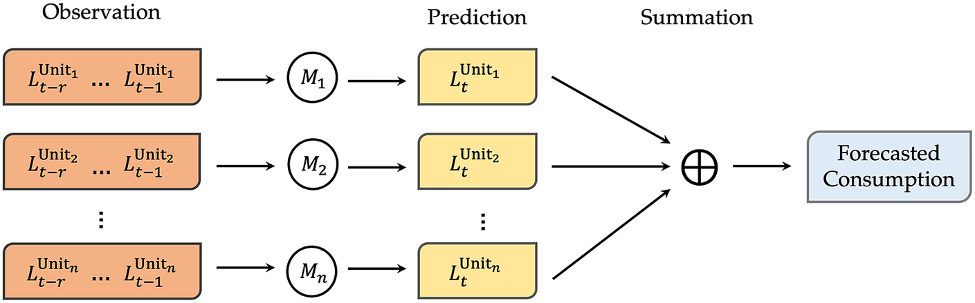
The bottom-up approach applied to load forecasting involves forecasting demand at each sub-aggregate level and then summing the sub-level forecasts to predict the aggregate demand. Figure 1 shows the schematic diagram of such a bottom-up approach, in which the goal is to predict the total demand for a group of $ n $
customer units. In this section, we discuss the two main challenges of the bottom-up approach: scalability and error propagation. We provide empirical demonstrations of how these challenges can lead to misleading results if not properly acknowledged.
$ n $
customer units. In this section, we discuss the two main challenges of the bottom-up approach: scalability and error propagation. We provide empirical demonstrations of how these challenges can lead to misleading results if not properly acknowledged.
The schematic diagram of the bottom-up approach, where $ {L}_t^{Unit_i} $
is the load (i.e., consumption) for
$ {L}_t^{Unit_i} $
is the load (i.e., consumption) for $ {i}^{th} $
unit at time
$ {i}^{th} $
unit at time $ t $
, and
$ t $
, and $ {M}_i $
is the model to predict
$ {M}_i $
is the model to predict $ {L}_t^{Unit_i} $
.
$ {L}_t^{Unit_i} $
.
2.1. Challenge of scalability
Consider $ n $
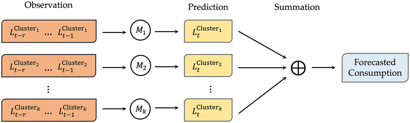
, the number of customer units in Figure 1 for which the total demand must be predicted, to be in the order of millions. It will, therefore, require the development of millions of prediction models. The process of performing meticulous model selection, calibration, and validation of these millions of individual models can be computationally cumbersome. To address this challenge, several studies have used the clustering-based bottom-up approach. Essentially, this entails first grouping the customer units into a handful of clusters, developing a prediction model for each cluster, and finally aggregating the predictions to obtain the total demand forecast. Figure 2 shows the schematic diagram of the clustering-based bottom-up approach.
$ n $
, the number of customer units in Figure 1 for which the total demand must be predicted, to be in the order of millions. It will, therefore, require the development of millions of prediction models. The process of performing meticulous model selection, calibration, and validation of these millions of individual models can be computationally cumbersome. To address this challenge, several studies have used the clustering-based bottom-up approach. Essentially, this entails first grouping the customer units into a handful of clusters, developing a prediction model for each cluster, and finally aggregating the predictions to obtain the total demand forecast. Figure 2 shows the schematic diagram of the clustering-based bottom-up approach.
The schematic diagram of the clustering-based bottom-up approach, where $ n $
customer units are grouped into
$ n $
customer units are grouped into $ k $
clusters, and
$ k $
clusters, and $ {L}_t^{Cluster_i} $
is the aggregated load (i.e., consumption) of units in the
$ {L}_t^{Cluster_i} $
is the aggregated load (i.e., consumption) of units in the $ {i}^{th} $
cluster at time
$ {i}^{th} $
cluster at time $ t $
, and
$ t $
, and $ {M}_i $
is the model to predict
$ {M}_i $
is the model to predict $ {L}_t^{Cluster_i} $
.
$ {L}_t^{Cluster_i} $
.
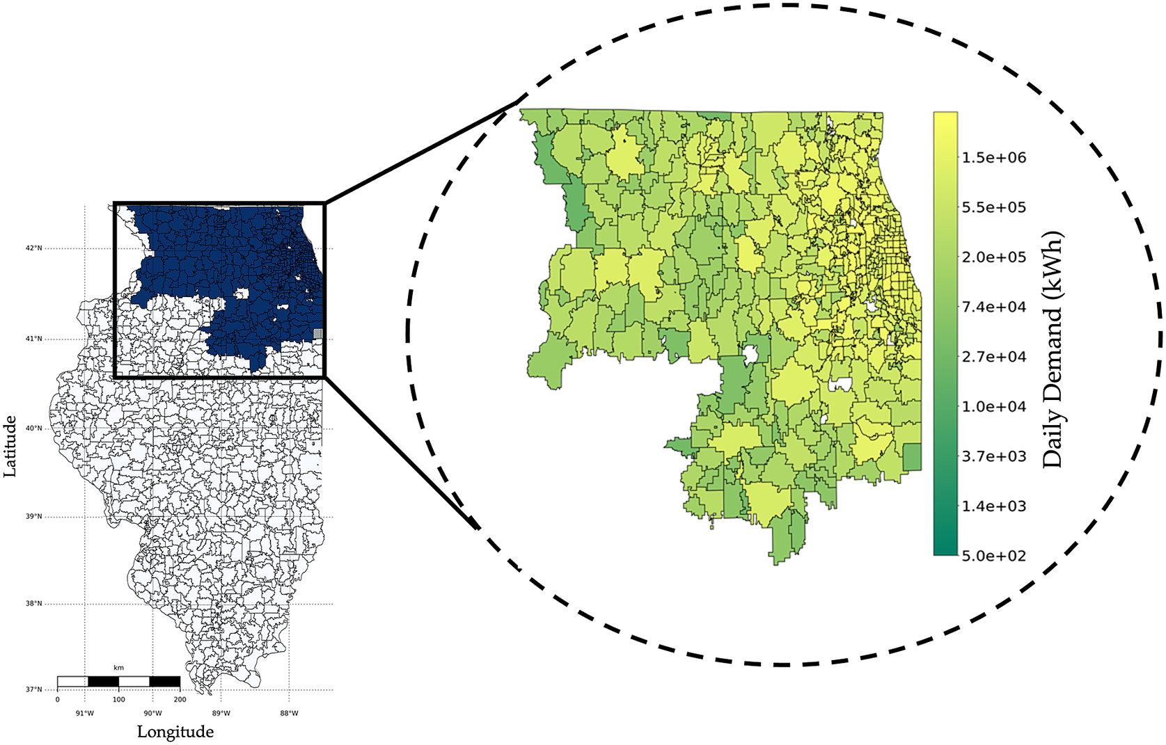
At first glance, it may seem that the clustering-based bottom-up approach can address scalability challenges. To understand the maximum scale of smart-meter data that has been handled using the clustering-based bottom-up approach, we take a closer look at the scale of the data used in studies that follow the clustering-based bottom-up approach to leverage smart-meter data in predicting the aggregate demand. Table 1 reveals applications to limited-size datasets, from a few hundred to a few thousand customers.
Size of smart-meter data used for demonstrating the application of the clustering-based bottom-up approach in predicting the aggregate demand.
The fact that the clustering-based bottom-up approach has not been used for large datasets is mostly because of the high computational cost of widely-applied clustering algorithms, such as $ K $
-means, which become computationally intractable when clustering fine-resolution smart-meter data from millions of customers is of interest (Mahdi et al., Reference Mahdi, Hosny and Elhenawy2021; Si et al., Reference Si, Xu, Wan, Chen, Cui and Zhao2021). Additionally, the amount of memory required to store the data in a format that is appropriate for clustering can quickly become prohibitive. Although more advanced clustering algorithms that take advantage of parallelization may alleviate the challenge to some extent, their implementation often involves complexities that prohibit their use by utility companies serving several million customers (Ding et al., Reference Ding, Wang, Dang, Fu, Zhang and Zhang2015; Hidri et al., Reference Hidri, Zoghlami and Ayed2018; Lei et al., Reference Lei, Jin, Hao and Li2019). Additionally, selecting the optimal number of clusters has been shown to significantly impact the accuracy of predictions (Alzate and Sinn, Reference Alzate and Sinn2013; Quilumba et al., Reference Quilumba, Lee, Huang, Wang and Szabados2014; Shahzadeh et al., Reference Shahzadeh, Khosravi and Nahavandi2015; Wijaya et al., Reference Wijaya, Vasirani, Humeau and Aberer2015; Wang et al., Reference Wang, Lee, Huang, Szabados, Wang and Van Olinda2016; Fahiman et al., Reference Fahiman, Erfani, Rajasegarar, Palaniswami and Leckie2017). The selection process, however, requires running the clustering algorithm several times for various numbers of clusters, a process that makes the clustering-based bottom-up approach even more computationally costly for millions of customers (Al Khafaf et al., Reference Al Khafaf, Jalili and Sokolowski2021).
$ K $
-means, which become computationally intractable when clustering fine-resolution smart-meter data from millions of customers is of interest (Mahdi et al., Reference Mahdi, Hosny and Elhenawy2021; Si et al., Reference Si, Xu, Wan, Chen, Cui and Zhao2021). Additionally, the amount of memory required to store the data in a format that is appropriate for clustering can quickly become prohibitive. Although more advanced clustering algorithms that take advantage of parallelization may alleviate the challenge to some extent, their implementation often involves complexities that prohibit their use by utility companies serving several million customers (Ding et al., Reference Ding, Wang, Dang, Fu, Zhang and Zhang2015; Hidri et al., Reference Hidri, Zoghlami and Ayed2018; Lei et al., Reference Lei, Jin, Hao and Li2019). Additionally, selecting the optimal number of clusters has been shown to significantly impact the accuracy of predictions (Alzate and Sinn, Reference Alzate and Sinn2013; Quilumba et al., Reference Quilumba, Lee, Huang, Wang and Szabados2014; Shahzadeh et al., Reference Shahzadeh, Khosravi and Nahavandi2015; Wijaya et al., Reference Wijaya, Vasirani, Humeau and Aberer2015; Wang et al., Reference Wang, Lee, Huang, Szabados, Wang and Van Olinda2016; Fahiman et al., Reference Fahiman, Erfani, Rajasegarar, Palaniswami and Leckie2017). The selection process, however, requires running the clustering algorithm several times for various numbers of clusters, a process that makes the clustering-based bottom-up approach even more computationally costly for millions of customers (Al Khafaf et al., Reference Al Khafaf, Jalili and Sokolowski2021).
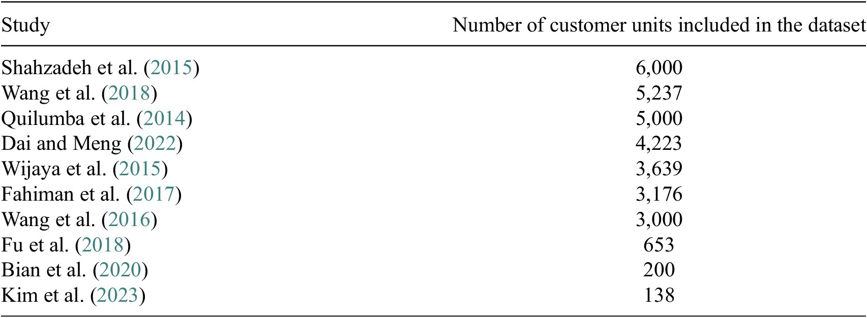
Consider a scenario where data from millions of customers is available. In such a scenario, optimal clustering of data is challenging to achieve in practice. In order to use the clustering-based bottom-up approach, one may use random clustering or natural clustering inherited from the data (e.g., grouping customer units based on their zip code). Such arbitrary clustering, however, can deteriorate forecast accuracy. We demonstrate this using data procured from Commonwealth Edison, commonly known as ComEd, which is the largest electric utility in the state of Illinois. ComEd serves more than 500 zip codes and 3.7 million customer units in Illinois; see Figure 3 for the service territory of ComEd.
The figure shows ComEd’s service area in Illinois, highlighted in dark, along with the daily demand for electricity (in kWh) in the company’s operational territory.
We use ComEd data to compare the accuracy offered by the clustering-based bottom-up approach versus an aggregated model that does not leverage fine-resolution data and simply predicts the total demand based on the previous observation of the aggregate demand. For the clustering-based bottom-up approach, in the absence of optimal clustering due to the extreme size of the data, we cluster the customer units based on their zip codes. We use demand data from October 2019 as an example of an uneventful month with no major holidays or climatic extremes to ensure a fair comparison of different approaches. The data is divided into a training set and a test set. The training set includes 80% of the available data, that is, the first 25 days of October. As shown in Figure 1, inputs to the models include the demand for $ r $
previous time steps. To obtain an optimum value for
$ r $
previous time steps. To obtain an optimum value for $ r $
, we use 80% of the data in the training set for training the predictive models with different values of
$ r $
, we use 80% of the data in the training set for training the predictive models with different values of $ r $
and perform validation using the remaining 20% of the data in the training set. Finally, the remaining 20% of the data (i.e., the last 6 days of October) is used as a test set to evaluate the models’ performance.
$ r $
and perform validation using the remaining 20% of the data in the training set. Finally, the remaining 20% of the data (i.e., the last 6 days of October) is used as a test set to evaluate the models’ performance.
Table 2 compares the mean absolute percentage error of bottom-up and aggregated model approaches for 30-min, 1-hr, and 2-hr load forecasting, using three distinctive classes of learning methods. Specifically, the aggregated model approach only takes the observed aggregate demand for the 3.7 customers to predict the next step demand. On the other hand, the clustering-based bottom-up approach develops a separate forecast model for each cluster of smart-meter data and uses the summation of forecasts to predict the next step of the aggregate demand. The use of different learning algorithms allows for ensuring the robustness of the results against the choice of learning technique. It must be noted that the goal is not to compare these three learning methods based on their accuracy. This is because a particular method’s performance is dependent on the characteristics of a data set. Here, the intent is to validate the independence of the results from the choice of the learning method. Specifically, it is observed that, regardless of the type of learning method, the bottom-up approach results in less accurate prediction compared to an aggregated model that does not leverage high-resolution data. Given the results in Table 2, it might be concluded that incorporating fine-resolution data does not improve the accuracy of the total demand prediction. It should however be noted that (1) the accuracy of the clustering-based bottom-up approach is highly dependent on optimal clustering, and (2) the bottom-up approach can result in large aggregated errors depending on the correlation of prediction errors at sub-aggregate levels.
Evaluated mean relative error in % for clustering-based bottom-up and aggregated approaches for 30-min, 1-hr, 2-hr prediction interval using three different prediction models.
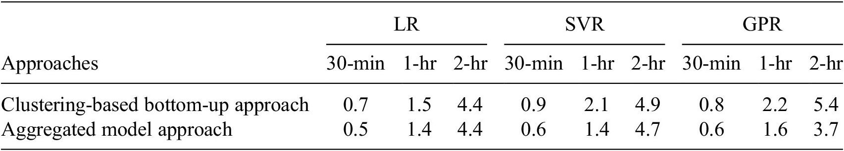
Note: LR, linear regression (Poole and O’Farrell, Reference Poole and O’Farrell1971); SVR, Support vector regression (Cortes and Vapnik, Reference Cortes and Vapnik1995); GPR, Gaussian process regression (Williams and Rasmussen, Reference Williams, Rasmussen, Touretzky, Mozer and Hasselmo1995).
Next, we discuss how the error aggregation challenge of the bottom-up approach has led to misleading results in the literature.
2.2. Challenge of error aggregation
With the rise of grid-interactive buildings and higher electrification of the building sector, predictive analytics for building-level energy consumption has attracted great attention in recent years. Advances in smart-metering technology and access to fine-resolution energy consumption data enable more accurate predictions. However, it is unclear whether fine-resolution data will always result in improved prediction accuracy. Addressing this gap is of high importance as collecting high-volume, fine-resolution data is resource-intensive and can overwhelm communication and storage systems. Jain et al. (Reference Jain, Smith, Culligan and Taylor2014) investigated the “optimal” temporal and spatial data granularity from the residential sector for accurate energy forecasting. They concluded that optimal monitoring granularity occurs at the floor level and at the hourly time interval. Their results show that collecting fine-resolution data (e.g., at the unit level and 10-min intervals) can significantly deteriorate prediction accuracy. However, in light of the fact that coarse-resolution data can be obtained by aggregating fine-resolution data, getting lower accuracy with fine-resolution data is counter-intuitive. In this work, we discuss how such misleading results are a function of using the bottom-up approach when it is not appropriate.
As illustrated in Figure 1, the bottom-up approach creates several forecasting models at a finer spatial granularity (e.g., apartment units) before aggregating them to evaluate a forecast at coarser spatial granularity (e.g., building). A major disadvantage of this type of bottom-up modeling is the potential for error aggregation (Schwarzkopf et al., Reference Schwarzkopf, Tersine and Morris1988; Hyndman et al., Reference Hyndman, Ahmed, Athanasopoulos and Shang2011). Specifically, assuming that the prediction errors for forecast models for different units are independent and follow $ \mathcal{N}(0,{\sigma}_i^2)\hskip0.1em $
, prediction error for the building will then follow
$ \mathcal{N}(0,{\sigma}_i^2)\hskip0.1em $
, prediction error for the building will then follow $ \mathcal{N}(0,{\sum}_{i=1}^n{\sigma}_i^2). $
Consequently, such a large variance may lead to highly inaccurate predictions. It is pertinent to note that the validity of the error independence assumption is problem-dependent and requires thorough investigation before employing the bottom-up approach.
$ \mathcal{N}(0,{\sum}_{i=1}^n{\sigma}_i^2). $
Consequently, such a large variance may lead to highly inaccurate predictions. It is pertinent to note that the validity of the error independence assumption is problem-dependent and requires thorough investigation before employing the bottom-up approach.
As an alternative, to avoid error aggregation, the fine-resolution data can directly be used as inputs to a single forecast model that predicts consumption at a coarse level, an approach we call the “single-model approach” (see Figure 4 for illustration).
The schematic diagram of the single-model approach, where $ {L}_t^{Unit_i} $
is the load (i.e., consumption) for
$ {L}_t^{Unit_i} $
is the load (i.e., consumption) for $ {i}^{th} $
unit at time
$ {i}^{th} $
unit at time $ t $
, and
$ t $
, and $ M $
is the model to predict the final load.
$ M $
is the model to predict the final load.

In this work, we seek to replicate the approach used in Jain et al. (Reference Jain, Smith, Culligan and Taylor2014) study and compare it with a single-model approach. Due to a lack of data from the original multi-residential building, we randomly sampled and analyzed data from 21 residential units located in a zip code covered by ComEd. We then assumed that the units belong to a six-story building, with six, four, three, three, three, and two units on each floor, similar to the distribution of units in Jain et al. (Reference Jain, Smith, Culligan and Taylor2014).
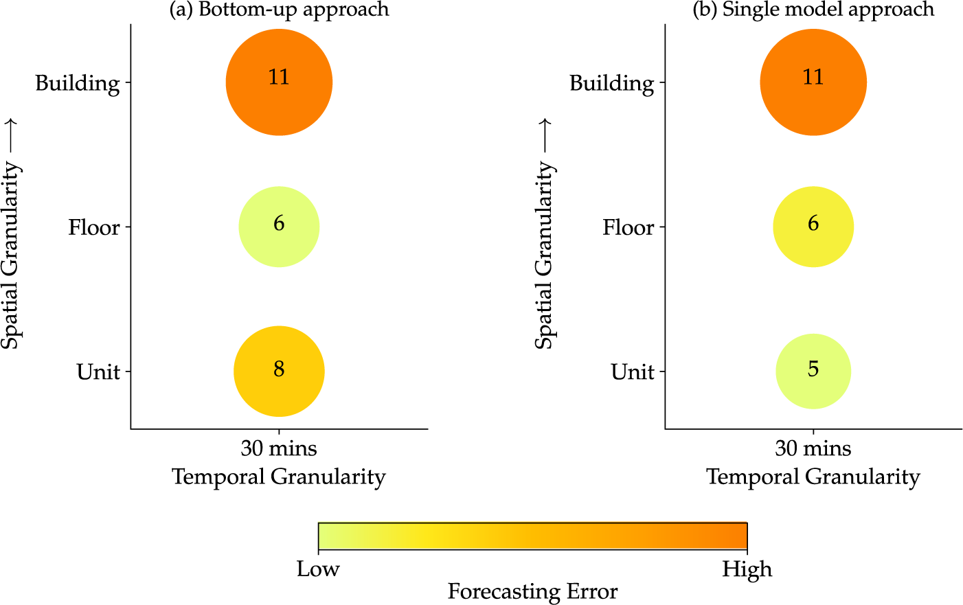
In this analysis, we compare forecasting errors between the two approaches based on different spatial granularities (units, floors, and buildings) at a fixed temporal granularity. In a similar manner to the setting in Jain et al. (Reference Jain, Smith, Culligan and Taylor2014), we employ support vector regression (SVR) with a Gaussian kernel as the learning algorithm, with the two most recent observations as the input of the model and the consumption at the next time step as the output. The relative prediction error for both approaches is shown in Figure 5. As data granularity increases from floor level to unit level, it becomes apparent that the bottom-up approach leads to higher error. Consequently, this may lead to a deceptive conclusion that collecting data at floor level provides optimal accuracy. In contrast, the higher error at the unit level is attributed to the large number of models that the bottom-up approach requires at such fine granularity. This is further confirmed by the fact that the single-model approach results in improved accuracy as fine-resolution data becomes available, which is in line with the intuitive pattern we expect.
Comparison of forecasting errors (in %) using SVR between two different modeling approaches, (a) bottom-up approach and (b) single-model approach, for a fixed temporal granularity.
It must be noted that as the size of fine-resolution smart-meter data increases, it most likely won’t be possible to directly incorporate data from all customer units as inputs into a single model. However, it has been shown that using hierarchical dimension-reduction approaches, high-dimensional smart-meter data can be transformed into low-dimensional space (Alemazkoor et al., Reference Alemazkoor, Tootkaboni, Nateghi and Louhghalam2022). The transformed low-dimensional data can be directly used as inputs to a single model. Specifically, Alemazkoor et al. (Reference Alemazkoor, Tootkaboni, Nateghi and Louhghalam2022) have shown that the single model approach that incorporated transformed data from smart-meter data of 3.7 million customer units performs better than the bottom-up approach, which is prone to scalability and error aggregation issues.
3. Discussion and Lessons Learned
3.1. Shortcomings of bottom-up approaches to harnessing big smart-meter data
Currently, (clustering-based) bottom-up approaches are state-of-the-art in the literature for exploiting fine-resolution smart-meter data in predicting aggregate demand. However, almost all (if not all) studies that have used the clustering-based bottom-up approach have demonstrated its ability to harness smart-meter data on rather small data sets (Alzate and Sinn, Reference Alzate and Sinn2013; Quilumba et al., Reference Quilumba, Lee, Huang, Wang and Szabados2014; Shahzadeh et al., Reference Shahzadeh, Khosravi and Nahavandi2015; Wijaya et al., Reference Wijaya, Vasirani, Humeau and Aberer2015; Wang et al., Reference Wang, Lee, Huang, Szabados, Wang and Van Olinda2016; Fahiman et al., Reference Fahiman, Erfani, Rajasegarar, Palaniswami and Leckie2017; Fu et al., Reference Fu, Zeng, Feng and Cai2018; Bian et al., Reference Bian, Zhong, Sun and Shi2020; Dai and Meng, Reference Dai and Meng2022; Kim et al., Reference Kim, Park and Kim2023). These studies are different in terms of their proposed clustering algorithms including $ k $
-means (Quilumba et al., Reference Quilumba, Lee, Huang, Wang and Szabados2014; Shahzadeh et al., Reference Shahzadeh, Khosravi and Nahavandi2015; Bian et al., Reference Bian, Zhong, Sun and Shi2020), kernel spectral (Alzate and Sinn, Reference Alzate and Sinn2013), and k-shape (Fahiman et al., Reference Fahiman, Erfani, Rajasegarar, Palaniswami and Leckie2017), and mainly focus on improving load forecast accuracy through optimal clustering (Wang et al., Reference Wang, Lee, Huang, Szabados, Wang and Van Olinda2016) and the use of advanced learning algorithms such as neural networks (Quilumba et al., Reference Quilumba, Lee, Huang, Wang and Szabados2014; Dagdougui et al., Reference Dagdougui, Bagheri, Le and Dessaint2019), deep learning (Fahiman et al., Reference Fahiman, Erfani, Rajasegarar, Palaniswami and Leckie2017; Bendaoud and Farah, Reference Bendaoud and Farah2020; Rafi et al., Reference Rafi, Nahid-Al-Masood, Deeba and Hossain2021), and hybrid methods (Singh et al., Reference Singh, Dwivedi and Kant2019; Aly, Reference Aly2020). These studies commonly lack discussions on the possibility of application of their proposed method to larger smart-meter data and the generalizability of their results. In fact, the most effective clustering method, the optimum number of clusters, and the ideal learning algorithm that yields the highest accuracy hinge on the characteristics of a particular dataset used in a study and may not be applicable to a different dataset (Temizel et al., Reference Temizel, Mizani, Inkaya and Yucebas2007; Jain et al., Reference Jain, Jain, AlSkaif and Dev2021). Moreover, even an algorithm that always performs well on small/medium size data may have poor performance on larger datasets. The lack of such transparent discussions in the literature is costly and troublesome. Specifically, in practice, blind applications of the proposed methods in the literature may result in misleading and sub-optimal results. As an example, it can be seen in Table 2 that using big smart-meter data from 3.7 million customer units in the bottom-up framework can result in less accurate load forecasts compared to the aggregated model approach that does not harness fine-resolution data at all. Such sub-optimal load forecasts not only lead to sub-optimal operation of the system but also waste all the efforts invested in the installation and maintenance of smart meters as well as data collection, cleaning, and processing.
$ k $
-means (Quilumba et al., Reference Quilumba, Lee, Huang, Wang and Szabados2014; Shahzadeh et al., Reference Shahzadeh, Khosravi and Nahavandi2015; Bian et al., Reference Bian, Zhong, Sun and Shi2020), kernel spectral (Alzate and Sinn, Reference Alzate and Sinn2013), and k-shape (Fahiman et al., Reference Fahiman, Erfani, Rajasegarar, Palaniswami and Leckie2017), and mainly focus on improving load forecast accuracy through optimal clustering (Wang et al., Reference Wang, Lee, Huang, Szabados, Wang and Van Olinda2016) and the use of advanced learning algorithms such as neural networks (Quilumba et al., Reference Quilumba, Lee, Huang, Wang and Szabados2014; Dagdougui et al., Reference Dagdougui, Bagheri, Le and Dessaint2019), deep learning (Fahiman et al., Reference Fahiman, Erfani, Rajasegarar, Palaniswami and Leckie2017; Bendaoud and Farah, Reference Bendaoud and Farah2020; Rafi et al., Reference Rafi, Nahid-Al-Masood, Deeba and Hossain2021), and hybrid methods (Singh et al., Reference Singh, Dwivedi and Kant2019; Aly, Reference Aly2020). These studies commonly lack discussions on the possibility of application of their proposed method to larger smart-meter data and the generalizability of their results. In fact, the most effective clustering method, the optimum number of clusters, and the ideal learning algorithm that yields the highest accuracy hinge on the characteristics of a particular dataset used in a study and may not be applicable to a different dataset (Temizel et al., Reference Temizel, Mizani, Inkaya and Yucebas2007; Jain et al., Reference Jain, Jain, AlSkaif and Dev2021). Moreover, even an algorithm that always performs well on small/medium size data may have poor performance on larger datasets. The lack of such transparent discussions in the literature is costly and troublesome. Specifically, in practice, blind applications of the proposed methods in the literature may result in misleading and sub-optimal results. As an example, it can be seen in Table 2 that using big smart-meter data from 3.7 million customer units in the bottom-up framework can result in less accurate load forecasts compared to the aggregated model approach that does not harness fine-resolution data at all. Such sub-optimal load forecasts not only lead to sub-optimal operation of the system but also waste all the efforts invested in the installation and maintenance of smart meters as well as data collection, cleaning, and processing.
3.2. Limitations of the bottom-up approach to building-level load forecasts
Even when scalability and the extremely large dimensionality of smart-meter data are not an issue, the bottom-up approach can lead to myopic results. Particularly, due to the error aggregation challenge associated with the bottom-up approach, the results from a high-impact paper by Jain et al. (Reference Jain, Smith, Culligan and Taylor2014)—with over 500 citations according to Google Scholar—suggest that incorporating fine-resolution data in building-level load forecasting may deteriorate forecast accuracy, which is counter-intuitive. It is possible that the results of such a high-impact study may discourage practitioners from acquiring high-resolution data without a deeper understanding of its potential advantages. In an attempt to replicate the results with a different dataset, we showed that, if leveraged properly, incorporating fine-resolution data improves forecast accuracy. Specifically, rather than the bottom-up approach, we employed the single-model approach that directly uses high-resolution data as inputs to predict building-level demand. It was observed that such a single-model approach allows better exploitation of detailed information inherent in high-resolution data in load forecasting (see Figure 5). It again highlights the importance of being aware of the limitations of the bottom-up approach before its implementation and using its results for deriving conclusions.
3.3. Application of bottom-up approaches
It should be emphasized that we do not oppose the use of the bottom-up method for load forecasting. Instead, we want to raise awareness about its shortcomings, as it has attracted considerable attention in the field of load forecasting. In fact, it is quite possible that for a specific dataset, the bottom-up approach works well. This can happen, for example, when the size of data allows optimal clustering, and prediction error for different sub-aggregate clusters has a small variance, leading to a small variance in aggregate prediction. The bottom-up approach can also provide insights into the behavior of each sub-aggregate group. However, when the goal is solely to forecast the aggregate demand, a comprehensive investigation of error aggregation possibility and comparison with the single-model approach is required before proceeding with the bottom-up approach.
4. Concluding Remarks
Through this work, we strive to raise awareness of the potential pitfalls associated with prefixed models among scientists working with data-driven models, as blindly applying any modeling approach can yield inaccurate and misleading results. Specifically, we focused on the application of the bottom-up approach in load forecasting and discussed how the lack of adequate acknowledgment of its shortcomings has led to methodologies that are not practical on a large scale or contribute to myopic results about the advantages of fine-resolution smart-meter data. In practice, such misleading results can have serious implications. On the surface, this can range from discouraging practitioners from seeking the tremendous value of big smart-meter data to picking a prediction model that is not compatible with fine-resolution big data and leads to sub-optimal predictions. Digging deeper, sub-optimal load forecasts arising from sub-utilization of fine-resolution load data can impose utility companies with excessive costs, given that a 1% increment in forecasting error costs utility companies between $300 thousand to $1.6 million annually (Hobbs et al., Reference Hobbs, Jitprapaikulsarn, Konda, Chankong, Loparo and Maratukulam1999; Hong, Reference Hong2015). This cost would be substantially higher for an intelligent distributed grid that mainly uses renewable energy sources and operates based on close interactions with consumers. Particularly, providing supply–demand balance in a carbon-neutral requires highly efficient load management, which can be hindered in the absence of highly accurate load forecasts. An imbalance between supply and demand can cause a waste of resources or blackouts with cascading effects and undesirable social, psychological, and physical outcomes, e.g., premature death, injury, and social unrest. Moreover, concerns about the availability of highly accurate load forecasts can further delay the clean energy transition, which has a critical role in combating climate change.
We hope that this work rectifies misleading messages about load forecasting using fine-resolution smart-meter data for the research community, practitioners, and decision-makers. Generally, the current age of big data has seen a proliferation of literature with studies that focus on a particular dataset to derive presumably generalizable conclusions. There are various conclusions, ranging from “Monitoring data at granularity $ X $
will provide the best accuracy for forecasting
$ X $
will provide the best accuracy for forecasting $ Y $
”, as suggested by Jain et al. (Reference Jain, Smith, Culligan and Taylor2014), to “Algorithm
$ Y $
”, as suggested by Jain et al. (Reference Jain, Smith, Culligan and Taylor2014), to “Algorithm $ Z $
provides the best accuracy for forecasting
$ Z $
provides the best accuracy for forecasting $ Y $
” in many scholarly works that focus on proposing a new forecasting method. As scientists, we need to seriously question the generalizability of such conclusions before trusting and building on them. In addition to being mindful of the inherent limitations of the methodology, we should also examine how results may vary depending on the characteristics of the particular data set being studied, such as data volume.
$ Y $
” in many scholarly works that focus on proposing a new forecasting method. As scientists, we need to seriously question the generalizability of such conclusions before trusting and building on them. In addition to being mindful of the inherent limitations of the methodology, we should also examine how results may vary depending on the characteristics of the particular data set being studied, such as data volume.
In light of the fact that many data-driven forecasting studies depend on a particular data set with non-generalizable results, the literature is in serious need of more methodology-based studies. As an example, the literature can benefit from studies that introduce alternatives to the bottom-up approach and discuss when and how the bottom-up approach or its alternative can be advantageous in harnessing fine-resolution data. This can include addressing how to deal with high-dimensional data when smart-meter data from numerous customer units are available, or how to quantify the trade-off between the increased accuracy and data collection cost when fine-resolution data is available. In other words, rather than prescribing a general approach to load forecasting, such a study would equip readers and researchers with tools they need for accurate load forecasting in the application area of their interest.
Author contribution
Conceptualization: R.N. and N.A.; Formal analysis: H.A.; Investigation: H.A. and N.A.; Methodology: H.A. and N.A.; Project administration: N.A.; Resources: N.A.; Supervision: N.A.; Software: H.A.; Validation: H.A. and N.A.; Visualization: H.A.; Writing—original draft: N.A.; Writing—review & editing: H.A., R.N. and N.A. All authors approved the final submitted draft.
Competing interest
The authors declare no competing interests.
Data availability statement
The code and data are available upon request.
Funding statement
This research did not receive any specific grant from funding agencies in the public, commercial, or not-for-profit sectors.


 Open access
Comments
No Comments have been published for this article.