


Impact Statement
Traditional Bayesian model calibration techniques can underestimate predictive uncertainty when the computational model cannot fully represent the observed data. This paper investigates how different likelihood formulations within an embedded model inadequacy framework influence the handling of measurement noise and model form uncertainties. The results highlight that the likelihood specification influences the posterior distribution, which subsequently governs the uncertainty propagated to predictions and unobserved QoIs. This provides valuable guidance for practitioners employing embedded model inadequacy in simulation-based calibration. By providing a more robust framework for managing uncertainties, this work advances the integration of simulations with measurement data, supporting practical applications such as digital twins.
1. Introduction
In the last few decades, advances in sensor technology have made available large quantities of affordable data that reflect the current state of physical systems and processes. In parallel, simulation models have become ubiquitous in science and engineering for generating predictions on the behavior of a given system based on physical laws. With the ongoing transition to an Industry 4.0 paradigm and the proliferation of Digital Twins, the challenge of calibrating simulation models based on data from physical sensors is becoming increasingly relevant (Vaidya et al., Reference Vaidya, Ambad and Bhosle2018). In the specific case of Digital Twins of physical systems that use simulations to predict the behavior of their real counterpart and make decisions on their behalf, the accuracy and reliability of such predictions are essential (Andrés Arcones et al., Reference Andrés Arcones, Weiser, Koutsourelakis and Unger2023). Therefore, their uncertainty must be adequately quantified to achieve such trustworthy predictions.
In most cases, the calibration of the computational models is achieved by estimating a set of parameters that control their behavior based on available observations from the modeled system. Although more uncertainty sources can be identified (Walker et al., Reference Walker, Harremoës, Rotmans, van der Sluijs, van Asselt, Janssen and Krayer von Krauss2003), this process introduces two main ones: the error attributed to noise or uncontrolled variations in the data and the discrepancy created by the assumptions used to generate the computational model. They can be related to aleatoric and epistemic uncertainty sources, respectively. While noise errors can be satisfactorily estimated from the observations, the so-called model discrepancy or model inadequacy presents further challenges. All models are based on assumptions and simplifications that are unavoidable when tackling an infinitely complex reality. Systematic reviews on different approaches for dealing with this model inadequacy exist (Campbell, Reference Campbell2006; Bojke et al., Reference Bojke, Claxton, Sculpher and Palmer2009; Gupta et al., Reference Gupta, Clark, Vrugt, Abramowitz and Ye2012; Pernot and Cailliez, Reference Pernot and Cailliez2017; Sung and Tuo, Reference Sung and Tuo2024), but they all coincide in the need for further research to achieve reliable methods for quantifying the model form uncertainty.
Bayesian approaches are usually implemented to infer the model parameters (Robert, Reference Robert2007; Gelman et al., Reference Gelman, Carlin, Stern, Dunson, Vehtari and Rubin2013), which allows for obtaining a probability distribution for those parameters based on the observed data. This distribution will narrow down to the optimal parameter value, which may not be able to represent the observations in the presence of model inadequacy (Kaipio and Somersalo, Reference Kaipio and Somersalo2006). One classical solution to this problem is the framework proposed by Kennedy and O’Hagan (Reference Kennedy and O’Hagan2001), which extends the model output with a flexible term that corrects the predictions to better reflect the observations. Since its conception, several extensions have been proposed within the framework (Bayarri et al., Reference Bayarri, Berger and Liu2009; Brynjarsdóttir and O’Hagan, Reference Brynjarsdóttir and O’Hagan2014; Plumlee, Reference Plumlee2017; Barbillon et al., Reference Barbillon, Forte and Paulo2024; Leoni et al., Reference Leoni, Maître, Rodio and Congedo2024). However, one key disadvantage of such implementations is the impossibility of transferring the inferred estimation of the model inadequacy term to other derived quantities of interest (QoI) computed with the same calibrated model (Andrés Arcones et al., Reference Andrés Arcones, Weiser, Koutsourelakis and Unger2024). In contrast to these external correction approaches that associate the uncertainty with the predictions from the model, internal corrections arise as an alternative by attributing the uncertainty to its components instead (Wu et al., Reference Wu, Levine, Schneider and Stuart2024). In this way, the inferred uncertainty can be pushed forward to any QoI that uses the same model parameters for its computation.
This family of approaches, also called parameter uncertainty inflation (PUI) methods (Pernot, Reference Pernot2017; Pernot and Cailliez, Reference Pernot and Cailliez2017) have been gaining traction in the last years. The most prominent approach is Sargsyan’s parameter embedding (Sargsyan et al., Reference Sargsyan, Najm and Ghanem2015, Reference Sargsyan, Huan and Najm2019), which adds a stochastic dimension to the variables to be inferred and fits it together with the other parameters. This methodology has been successfully implemented in the context of ignition reaction (Huan et al., Reference Huan, Safta, Sargsyan, Geraci, Eldred, Vane, Lacazek, Oefelein and Najm2017). As alternatives to this methodology, Mortensen et al. (Reference Mortensen, Kaasbjerg, Frederiksen, Nørskov, Sethna and Jacobsen2005) proposes the statistical manipulation of the inferred parameter variance, and Wu et al. (Reference Wu, Levine, Schneider and Stuart2024) suggests inferring the internal model error structure through Kalman filters.
Alternatively, and related to these internal correction strategies, Stochastic Model Updating (SMU) methods have been developed to jointly address aleatory and epistemic uncertainties by updating the probabilistic descriptions of model parameters based on discrepancies between simulations and experimental data. These methods typically require multiple observations per prediction point to separate the two uncertainty sources and to estimate probability distributions directly. For example, Bi et al. (Reference Bi, Broggi and Beer2019) proposed an SMU framework based on the Bhattacharyya distance within an Approximate Bayesian Computation (ABC) setting, while Lee et al. (Reference Lee, Yaoyama, Kitahara and Itoi2025) introduced a latent-space-based SMU formulation that leverages variational autoencoders to handle high-dimensional data efficiently. In contrast, the embedded model inadequacy framework adopted in this work does not require multiple observations to account for the epistemic uncertainty, as the aleatoric part is prescribed or inferred as a parameter. This distinction makes the embedded approach particularly suited to simulation-based model calibration problems where repeated experimental measurements are rarely feasible.
The aforementioned formulations have the advantage of offering a flexible implementation that can be adapted to the requirements of the problem. Despite being the most promising approach for dealing with model error through an internal correction, Sargsyan’s proposal requires further refinement for complex inference cases (Pernot, Reference Pernot2017). This paper aims to address the challenges that arise when using the embedded approach for the calibration of simulation models from sensor data, and in particular a) the impact of misspecified noise models, b) the presence of observations that cannot be explained with modifications of the estimated parameters, and c) how the choice of likelihood affects the uncertainty propagation to other QoIs. A modification in how the prescribed noise is handled is introduced in the two main likelihood formulations proposed in Sargsyan et al. (Reference Sargsyan, Najm and Ghanem2015) for the embedded problem—the Independent Normal (IN) and Approximate Bayesian Computation (ABC) likelihoods. The IN likelihood tends to overemphasize low variance locations (Sargsyan et al., Reference Sargsyan, Najm and Ghanem2015) and it will be shown that ABC is specially sensitive to misspecified noise and locations where the model discrepancy cannot be reduced by variations in the parameters. Two new formulations based on the statistical convergence of the residual distribution aimed to alleviate the flaws of IN and ABC are proposed in this paper: the Global Moment-matching (GMM) and Relative Global Moment-matching (RGMM) likelihoods. Further insight is provided for the choice in the control parameters of the likelihoods and their potential shortcomings. Finally, an analysis of the propagation of the uncertainties through QoI is developed. The QoIs obtained from the computational model are observed by virtual sensors (Andrés Arcones et al., Reference Andrés Arcones, Weiser, Koutsourelakis and Unger2023). In contrast with real sensors that are installed in the physical system, virtual sensors observe values provided by the computational model. They are not limited to observable quantities as the real sensors, but can represent any QoI. Quantifying the uncertainty in the output of virtual sensors is key for an assessment of the reliability of the predictions of QoIs.
The advantages and disadvantages of each formulation will first be illustrated on a one-dimensional, linear example with different variations that reflect the possible errors in the observations. Afterwards, a more complex transient thermal model simulating the heat transfer through a reinforced concrete structure is investigated. The objective of the more complex case is to test the propagation of the inferred uncertainty using each different likelihood to a non-related QoI. The structure of the rest of the paper is as follows: Section 2 presents the embedded approach, the likelihood functions and the proposed extensions, Section 3 includes the simple, linear model with its variations (Section 3.1) and the complex transient thermal one (Section 3.2), and conclusions and possible extensions are provided in Section 4. The methods here implemented are included in the Python package probeye ([dataset] BAMResearch, 2024).
2. Methodology
2.1. Model form uncertainty framework
Let
 $ f $
be a computable, deterministic function
$ f $
be a computable, deterministic function
 $ f:\Theta \times {\mathrm{\mathbb{R}}}^{n_x}\to {\mathrm{\mathbb{R}}}^{n_z} $
for a
$ f:\Theta \times {\mathrm{\mathbb{R}}}^{n_x}\to {\mathrm{\mathbb{R}}}^{n_z} $
for a
 $ {n}_x $
-dimensional input
$ {n}_x $
-dimensional input
 $ x\in {\mathrm{\mathbb{R}}}^{n_x} $
, parametrized through a set of
$ x\in {\mathrm{\mathbb{R}}}^{n_x} $
, parametrized through a set of
 $ {n}_{\theta } $
parameters
$ {n}_{\theta } $
parameters
 $ \boldsymbol{\theta} \in \Theta \subseteq {\mathrm{\mathbb{R}}}^{n_{\theta }} $
, which have been restricted to real values for simplicity. This function
$ \boldsymbol{\theta} \in \Theta \subseteq {\mathrm{\mathbb{R}}}^{n_{\theta }} $
, which have been restricted to real values for simplicity. This function
 $ f $
models the real response
$ f $
models the real response
 $ z:{\mathrm{\mathbb{R}}}^{n_x}\to {\mathrm{\mathbb{R}}}^{n_z} $
, defined as a real-valued map that generates the
$ z:{\mathrm{\mathbb{R}}}^{n_x}\to {\mathrm{\mathbb{R}}}^{n_z} $
, defined as a real-valued map that generates the
 $ {n}_z $
-dimensional response of a real system. In that case, an additional error term
$ {n}_z $
-dimensional response of a real system. In that case, an additional error term
 $ {\varepsilon}_{\mathrm{model}}=z-f $
rooted in the inability of
$ {\varepsilon}_{\mathrm{model}}=z-f $
rooted in the inability of
 $ f $
to exactly reproduce
$ f $
to exactly reproduce
 $ z $
is introduced. This model inadequacy term
$ z $
is introduced. This model inadequacy term
 $ {\varepsilon}_{\mathrm{model}} $
will be referred to as model form uncertainty. If the same response is measured through sensor observations
$ {\varepsilon}_{\mathrm{model}} $
will be referred to as model form uncertainty. If the same response is measured through sensor observations
 $ y $
, a noise
$ y $
, a noise
 $ {\varepsilon}_{\mathrm{noise}} $
will introduce an additional model inadequacy with
$ {\varepsilon}_{\mathrm{noise}} $
will introduce an additional model inadequacy with
 $ z $
. The measurement noise
$ z $
. The measurement noise
 $ {\varepsilon}_{\mathrm{noise}} $
is typically prescribed by the sensor manufacturer, often assuming an additive, homoscedastic Gaussian error model with known variance
$ {\varepsilon}_{\mathrm{noise}} $
is typically prescribed by the sensor manufacturer, often assuming an additive, homoscedastic Gaussian error model with known variance
 $ {\left({\sigma}_N\right)}^2 $
, whereas in other situations, its statistical properties are estimated directly from repeated or reference data observations. In this work, we generally adopt the former case unless explicitly stated otherwise, as it enables a tractable analytical treatment of the noise contribution consistent with the objectives of this study. The relation between observations and computational model predictions can be expressed as
$ {\left({\sigma}_N\right)}^2 $
, whereas in other situations, its statistical properties are estimated directly from repeated or reference data observations. In this work, we generally adopt the former case unless explicitly stated otherwise, as it enables a tractable analytical treatment of the noise contribution consistent with the objectives of this study. The relation between observations and computational model predictions can be expressed as
 $$ y=z(x)+{\varepsilon}_{\mathrm{noise}}=f\left(\theta, x\right)+{\varepsilon}_{\mathrm{model}}+{\varepsilon}_{\mathrm{noise}}, $$
modeling the model inadequacy terms additively. This formulation was introduced in the seminal paper of Kennedy and O’Hagan (Reference Kennedy and O’Hagan2001), where they state the need for including the model error in the calibration of computational models. Alternative formulations are possible, such as a multiplicative relation between model inadequacy terms and model predictions.
The objective of the so-called inverse problem is to estimate the values for the parameters
 $ {\boldsymbol{\theta}}^{\ast} $
such that
$ {\boldsymbol{\theta}}^{\ast} $
such that
 $ f $
best approximates
$ f $
best approximates
 $ z $
as
$ z $
as
 $$ {\boldsymbol{\theta}}^{\ast}=\arg \underset{\boldsymbol{\theta} \in \Theta}{\min}\left\Vert z-f\left(\theta, \cdot \right)\right\Vert, $$
where
 $ \parallel \cdot \parallel $
is a distance to be defined later. As
$ \parallel \cdot \parallel $
is a distance to be defined later. As
 $ z $
is not generally known, it is commonly substituted by the set of
$ z $
is not generally known, it is commonly substituted by the set of
 $ {n}_y $
sensor observations
$ {n}_y $
sensor observations
 $ \boldsymbol{y} $
for known input parameters
$ \boldsymbol{y} $
for known input parameters
 $ \boldsymbol{x} $
, where bold notation will be used to denote vector quantities. The inverse problem then transforms to
$ \boldsymbol{x} $
, where bold notation will be used to denote vector quantities. The inverse problem then transforms to
 $$ {\boldsymbol{\theta}}^{\ast}=\arg \underset{\boldsymbol{\theta} \in \Theta}{\min}\left\Vert \boldsymbol{y}-f\left(\theta, \boldsymbol{x}\right)\right\Vert . $$
Bayesian approaches are a popular choice to solve the inverse problem (Kaipio and Somersalo, Reference Kaipio and Somersalo2006). They provide a posterior probability density
 $ \pi \left(\boldsymbol{\theta} |\boldsymbol{y}\right) $
on the parameters
$ \pi \left(\boldsymbol{\theta} |\boldsymbol{y}\right) $
on the parameters
 $ \boldsymbol{\theta} $
given the observations
$ \boldsymbol{\theta} $
given the observations
 $ \boldsymbol{y} $
and the computational model
$ \boldsymbol{y} $
and the computational model
 $ \boldsymbol{f}\left(\boldsymbol{\theta}, \boldsymbol{x}\right) $
. The application of Bayes’ theorem yields
$ \boldsymbol{f}\left(\boldsymbol{\theta}, \boldsymbol{x}\right) $
. The application of Bayes’ theorem yields
 $$ \pi \left(\boldsymbol{\theta} |\boldsymbol{y}\right)=\frac{\pi \left(\boldsymbol{\theta} \right)\pi \left(\boldsymbol{y}|\boldsymbol{\theta} \right)}{\pi \left(\boldsymbol{y}\right)} $$
where
 $ \pi \left(\boldsymbol{\theta} |\boldsymbol{y}\right) $
is the posterior probability distribution,
$ \pi \left(\boldsymbol{\theta} |\boldsymbol{y}\right) $
is the posterior probability distribution,
 $ \pi \left(\boldsymbol{\theta} \right) $
is the prior probability distribution that encompasses the previous knowledge on the unknown parameters,
$ \pi \left(\boldsymbol{\theta} \right) $
is the prior probability distribution that encompasses the previous knowledge on the unknown parameters,
 $ \pi \left(\boldsymbol{y}|\boldsymbol{\theta} \right) $
is the likelihood of the observations
$ \pi \left(\boldsymbol{y}|\boldsymbol{\theta} \right) $
is the likelihood of the observations
 $ \boldsymbol{y} $
having been generated by
$ \boldsymbol{y} $
having been generated by
 $ \boldsymbol{\theta} $
and
$ \boldsymbol{\theta} $
and
 $ \pi \left(\boldsymbol{y}\right) $
is the marginal probability distribution of the observations. We assume the prior distribution
$ \pi \left(\boldsymbol{y}\right) $
is the marginal probability distribution of the observations. We assume the prior distribution
 $ \pi \left(\boldsymbol{\theta} \right) $
to be given, such that the remaining key challenge is the choice and evaluation of the likelihood function
$ \pi \left(\boldsymbol{\theta} \right) $
to be given, such that the remaining key challenge is the choice and evaluation of the likelihood function
 $ \mathcal{L}\left(\boldsymbol{\theta} \right)=\pi \left(\boldsymbol{y}|\boldsymbol{\theta} \right) $
for the given set of observations
$ \mathcal{L}\left(\boldsymbol{\theta} \right)=\pi \left(\boldsymbol{y}|\boldsymbol{\theta} \right) $
for the given set of observations
 $ \boldsymbol{y} $
. Bayesian inference approaches are based on the evaluation of the relationship from Equation 4 to obtain the posterior distribution of the unknown parameters
$ \boldsymbol{y} $
. Bayesian inference approaches are based on the evaluation of the relationship from Equation 4 to obtain the posterior distribution of the unknown parameters
 $ \boldsymbol{\theta} $
.
$ \boldsymbol{\theta} $
.
Once the posterior distribution of the unknown parameters is obtained, it can be pushed forward to generate predictions
 $ {\boldsymbol{f}}_P\left(\boldsymbol{\theta}, \boldsymbol{x}|\boldsymbol{y}\right) $
using the same forward model
$ {\boldsymbol{f}}_P\left(\boldsymbol{\theta}, \boldsymbol{x}|\boldsymbol{y}\right) $
using the same forward model
 $ f $
or they can be used in a different model
$ f $
or they can be used in a different model
 $ g\left(\boldsymbol{\theta} \right):\Theta \to \mathrm{\mathbb{R}} $
, for example, that computes a QoI using the same model parameters but evaluating a different quantity. In the first case
$ g\left(\boldsymbol{\theta} \right):\Theta \to \mathrm{\mathbb{R}} $
, for example, that computes a QoI using the same model parameters but evaluating a different quantity. In the first case
 $ {\boldsymbol{f}}_P\left(\boldsymbol{\theta}, \boldsymbol{x}|\boldsymbol{y}\right) $
can usually be compared with
$ {\boldsymbol{f}}_P\left(\boldsymbol{\theta}, \boldsymbol{x}|\boldsymbol{y}\right) $
can usually be compared with
 $ \boldsymbol{y} $
and indirectly
$ \boldsymbol{y} $
and indirectly
 $ \boldsymbol{z}\left(\boldsymbol{x}\right) $
through
$ \boldsymbol{z}\left(\boldsymbol{x}\right) $
through
 $ {\varepsilon}_{\mathrm{noise}} $
.
$ {\varepsilon}_{\mathrm{noise}} $
.
The calculation of
 $ \mathcal{L}\left(\boldsymbol{\theta} \right) $
requires the evaluation of the computational model
$ \mathcal{L}\left(\boldsymbol{\theta} \right) $
requires the evaluation of the computational model
 $ f $
under the assumption that it generates the real system’s response
$ f $
under the assumption that it generates the real system’s response
 $ z $
. However, that is not generally the case and the model error must be considered. Kennedy and O’Hagan (Reference Kennedy and O’Hagan2001) propose to include the model form uncertainty
$ z $
. However, that is not generally the case and the model error must be considered. Kennedy and O’Hagan (Reference Kennedy and O’Hagan2001) propose to include the model form uncertainty
 $ {\varepsilon}_{\mathrm{model}} $
in the inference procedure, formulated as a Gaussian Process added to the predicted response as in Equation 1. Despite its potential applications, this model’s inadequacy term lacks physical meaning and cannot be employed outside of the use case with which it is inferred. Therefore, the uncertainty quantified by
$ {\varepsilon}_{\mathrm{model}} $
in the inference procedure, formulated as a Gaussian Process added to the predicted response as in Equation 1. Despite its potential applications, this model’s inadequacy term lacks physical meaning and cannot be employed outside of the use case with which it is inferred. Therefore, the uncertainty quantified by
 $ {\varepsilon}_{\mathrm{model}} $
cannot be propagated to other QoI through the model
$ {\varepsilon}_{\mathrm{model}} $
cannot be propagated to other QoI through the model
 $ g $
. Notice that this model inadequacy term does not aim to identify the deficiencies in the model and correct them, but to introduce a term that envelops their effects, such that the response is corrected.
$ g $
. Notice that this model inadequacy term does not aim to identify the deficiencies in the model and correct them, but to introduce a term that envelops their effects, such that the response is corrected.
More importantly, adding the model inadequacy term to the predicted outputs does not address one of the main challenges of using classical Bayesian inference approaches with imperfect models: the posterior distributions of the unknown parameters collapse to Dirac-delta distributions, which produce model responses that do not correspond with the system that generated the observation. This is commonly known as the problem of misspecification. The Bernstein–von Mises theorem states that under a set of conditions of continuity, differentiability and non-singularity, the posterior distribution
 $ \pi \left(\boldsymbol{\theta} |\boldsymbol{y}\right) $
converges in total variation (TV) distance with the true generating process
$ \pi \left(\boldsymbol{\theta} |\boldsymbol{y}\right) $
converges in total variation (TV) distance with the true generating process
 $ {\pi}_{{\boldsymbol{\theta}}_0} $
to a multivariate normal distribution centered at the maximum likelihood estimator (MLE)
$ {\pi}_{{\boldsymbol{\theta}}_0} $
to a multivariate normal distribution centered at the maximum likelihood estimator (MLE)
 $ \hat{\boldsymbol{\theta}} $
and covariance matrix
$ \hat{\boldsymbol{\theta}} $
and covariance matrix
 $ {\left({n}_y\right)}^{-1}\mathcal{I}{\left({\boldsymbol{\theta}}_0\right)}^{-1} $
. Here,
$ {\left({n}_y\right)}^{-1}\mathcal{I}{\left({\boldsymbol{\theta}}_0\right)}^{-1} $
. Here,
 $ {n}_y $
is the number of observations in
$ {n}_y $
is the number of observations in
 $ \boldsymbol{y} $
and
$ \boldsymbol{y} $
and
 $ \mathcal{I}\left({\boldsymbol{\theta}}_0\right) $
is Fisher’s information matrix at the true values
$ \mathcal{I}\left({\boldsymbol{\theta}}_0\right) $
is Fisher’s information matrix at the true values
 $ {\boldsymbol{\theta}}_0 $
of the unknown parameters (van der Vaart, Reference van der Vaart2000). Formally, this can be formulated as
$ {\boldsymbol{\theta}}_0 $
of the unknown parameters (van der Vaart, Reference van der Vaart2000). Formally, this can be formulated as
 $$ {\left\Vert \pi \left(\boldsymbol{\theta} |\boldsymbol{y}\right)-\mathcal{N}\Big(\hat{\boldsymbol{\theta}},{\left({n}_y\right)}^{-1}\mathcal{I}{\left({\boldsymbol{\theta}}_0\right)}^{-1}\Big)\right\Vert}_{TV}\overset{\pi_{{\boldsymbol{\theta}}_0}}{\to }0. $$
This result is crucial for constructing confidence intervals for the parameters and predictive responses, linking Bayesian and frequentist statistics. For large values of
 $ {n}_y $
, the posterior distribution becomes concentrated around the MLE
$ {n}_y $
, the posterior distribution becomes concentrated around the MLE
 $ \hat{\boldsymbol{\theta}} $
. However, Kleijn and van der Vaart (Reference Kleijn and van der Vaart2012) demonstrated that the confidence intervals derived from Bernstein–von Mises theorem application only reflect the real credibility of the predictions in the case of perfect models that can reproduce the observations exactly.
$ \hat{\boldsymbol{\theta}} $
. However, Kleijn and van der Vaart (Reference Kleijn and van der Vaart2012) demonstrated that the confidence intervals derived from Bernstein–von Mises theorem application only reflect the real credibility of the predictions in the case of perfect models that can reproduce the observations exactly.
In the case of imperfect models, where discrepancies exist between the model and the data, the posterior distribution still converges to a multivariate normal distribution that concentrates around the MLE
 $ \hat{\boldsymbol{\theta}} $
for large
$ \hat{\boldsymbol{\theta}} $
for large
 $ {n}_y $
. However,
$ {n}_y $
. However,
 $ \hat{\boldsymbol{\theta}} $
may not generate the observations due to the model inadequacy, even for large
$ \hat{\boldsymbol{\theta}} $
may not generate the observations due to the model inadequacy, even for large
 $ {n}_y $
, and therefore the associated confidence intervals for the predictive response cannot be interpreted as credible intervals with respect to the true system, as demonstrated by Kleijn and van der Vaart (Reference Kleijn and van der Vaart2012). This implies that the predicted distributions do not adequately capture the variability of the true system, making them unsuitable for quantifying system uncertainty.
$ {n}_y $
, and therefore the associated confidence intervals for the predictive response cannot be interpreted as credible intervals with respect to the true system, as demonstrated by Kleijn and van der Vaart (Reference Kleijn and van der Vaart2012). This implies that the predicted distributions do not adequately capture the variability of the true system, making them unsuitable for quantifying system uncertainty.
When the model inadequacy vector
 $ {\delta}_{\mathrm{model}} $
, that models
$ {\delta}_{\mathrm{model}} $
, that models
 $ {\varepsilon}_{\mathrm{model}} $
at the observation points, is implemented as a correction to the model response, the combined model
$ {\varepsilon}_{\mathrm{model}} $
at the observation points, is implemented as a correction to the model response, the combined model
 $ {\boldsymbol{f}}_P+{\delta}_{\mathrm{model}} $
can reproduce exactly the observations
$ {\boldsymbol{f}}_P+{\delta}_{\mathrm{model}} $
can reproduce exactly the observations
 $ \mathbf{y} $
. As a result, the Bernstein–von Mises theorem holds within the domain of the parameters updated during this process. However, the model
$ \mathbf{y} $
. As a result, the Bernstein–von Mises theorem holds within the domain of the parameters updated during this process. However, the model
 $ {\boldsymbol{f}}_P $
alone cannot reliably quantify uncertainty without correcting the
$ {\boldsymbol{f}}_P $
alone cannot reliably quantify uncertainty without correcting the
 $ {\varepsilon}_{\mathrm{model}} $
, as it is limited to the observations’ domain. Similar to the scenario where no model inadequacy term is used, the model produces overly concentrated posterior distributions for both the parameters and the response, which may fail to represent the observations accurately. As the computation of QoIs through
$ {\varepsilon}_{\mathrm{model}} $
, as it is limited to the observations’ domain. Similar to the scenario where no model inadequacy term is used, the model produces overly concentrated posterior distributions for both the parameters and the response, which may fail to represent the observations accurately. As the computation of QoIs through
 $ g\left(\boldsymbol{\theta} \right) $
usually depends only on the parameters and not on the corrected model response
$ g\left(\boldsymbol{\theta} \right) $
usually depends only on the parameters and not on the corrected model response
 $ {\boldsymbol{f}}_P+{\varepsilon}_{\mathrm{model}} $
, the uncertainty in the QoI will not be representative of the credibility of the model.
$ {\boldsymbol{f}}_P+{\varepsilon}_{\mathrm{model}} $
, the uncertainty in the QoI will not be representative of the credibility of the model.
A promising solution to these challenges is the use of an embedded formulation where the inadequacy is added to the model through the unknown parameters. The objective is to augment those parameters with an additional stochastic variable that introduces random variations in the pre-existing model parameters. It is the introduction of this variability what prevents the unknown parameters from presenting a concentrated posterior for large
 $ {n}_y $
. Following the same philosophy as Kennedy and O’Hagan’s (KOH) framework, no corrections are introduced in the structure of the physical model which allows the approach to be used non-intrusively with parametrized black-box models. This embedding is presented through Sections 2.2 to 2.4, the likelihood definition and evaluation in Sections 2.5 and 2.6, and the calculation of predicted variables through
$ {n}_y $
. Following the same philosophy as Kennedy and O’Hagan’s (KOH) framework, no corrections are introduced in the structure of the physical model which allows the approach to be used non-intrusively with parametrized black-box models. This embedding is presented through Sections 2.2 to 2.4, the likelihood definition and evaluation in Sections 2.5 and 2.6, and the calculation of predicted variables through
 $ {\boldsymbol{f}}_P $
and QoIs through
$ {\boldsymbol{f}}_P $
and QoIs through
 $ g $
are presented in Section 2.7.
$ g $
are presented in Section 2.7.
2.2. Embedding of model form uncertainty
The objective of the embedding is that, despite the unavoidable collapse of the posterior distributions of the unknown parameters to Dirac-deltas, the distribution of the response should preserve the variance present in the observations. This is achieved by treating the unknown parameters
 $ \boldsymbol{\theta} $
as random variables with known distributions. The objective is now to infer the values of the parameters of the distribution. We will denote these random variables as
$ \boldsymbol{\theta} $
as random variables with known distributions. The objective is now to infer the values of the parameters of the distribution. We will denote these random variables as
 $ \tilde{\boldsymbol{\theta}} $
. This idea is similar to the one employed in hierarchical Bayesian approaches, where the prior distribution of
$ \tilde{\boldsymbol{\theta}} $
. This idea is similar to the one employed in hierarchical Bayesian approaches, where the prior distribution of
 $ \boldsymbol{\theta} $
is unknown. This turns the originally deterministic model into a stochastic one. With this approach, the extended model’s response
$ \boldsymbol{\theta} $
is unknown. This turns the originally deterministic model into a stochastic one. With this approach, the extended model’s response
 $ f\left(\tilde{\boldsymbol{\theta}}\right) $
does not necessarily collapse to a Dirac-delta distribution, as a given sample of the inferred parameters still generates a non-concentrated distribution of the random variable
$ f\left(\tilde{\boldsymbol{\theta}}\right) $
does not necessarily collapse to a Dirac-delta distribution, as a given sample of the inferred parameters still generates a non-concentrated distribution of the random variable
 $ \tilde{\boldsymbol{\theta}} $
.
$ \tilde{\boldsymbol{\theta}} $
.
There are different ways to model the random vector
 $ \tilde{\boldsymbol{\theta}} $
. One well-known approach, employed in Sargsyan et al. (Reference Sargsyan, Najm and Ghanem2015, Reference Sargsyan, Huan and Najm2019), uses Polynomial Chaos Expansions (PCE) to represent the stochastic, unknown parameters. Specifically, the parameter vector
$ \tilde{\boldsymbol{\theta}} $
. One well-known approach, employed in Sargsyan et al. (Reference Sargsyan, Najm and Ghanem2015, Reference Sargsyan, Huan and Najm2019), uses Polynomial Chaos Expansions (PCE) to represent the stochastic, unknown parameters. Specifically, the parameter vector
 $ \tilde{\boldsymbol{\theta}} $
is expressed as a series expansion as
$ \tilde{\boldsymbol{\theta}} $
is expressed as a series expansion as
 $$ \tilde{\boldsymbol{\theta}}\sim \sum \limits_j{\alpha}_j{\Psi}_j\left(\boldsymbol{\xi} \right), $$
where
 $ {\alpha}_j\in {\mathrm{\mathbb{R}}}^{n_{\theta }} $
are the expansion’s coefficients (included in the unknown parameter space
$ {\alpha}_j\in {\mathrm{\mathbb{R}}}^{n_{\theta }} $
are the expansion’s coefficients (included in the unknown parameter space
 $ \Theta $
),
$ \Theta $
),
 $ {\Psi}_j:{\mathrm{\mathbb{R}}}^{n_{\xi }}\to \mathrm{\mathbb{R}} $
are orthogonal polynomials, and
$ {\Psi}_j:{\mathrm{\mathbb{R}}}^{n_{\xi }}\to \mathrm{\mathbb{R}} $
are orthogonal polynomials, and
 $ \boldsymbol{\xi} $
is a set of stochastic variables (also called the stochastic germ) with
$ \boldsymbol{\xi} $
is a set of stochastic variables (also called the stochastic germ) with
 $ \boldsymbol{\xi} \in {\mathrm{\mathbb{R}}}_{\xi}^n $
where
$ \boldsymbol{\xi} \in {\mathrm{\mathbb{R}}}_{\xi}^n $
where
 $ {n}_{\xi } $
is the number of input random variables considered. This PCE-based approach allows for a flexible representation of the distribution of
$ {n}_{\xi } $
is the number of input random variables considered. This PCE-based approach allows for a flexible representation of the distribution of
 $ \tilde{\boldsymbol{\theta}} $
.
$ \tilde{\boldsymbol{\theta}} $
.
In this paper, instead of representing
 $ \tilde{\boldsymbol{\theta}} $
as a polynomial expansion, we adopt an explicit representation where the stochasticity is introduced through an additive model inadequacy term. This approach is in line with the proposal of Oliver et al. (Reference Oliver, Terejanu, Simmons and Moser2015) for model error characterization and the work of Strong and Oakley (Reference Strong and Oakley2014) on internal model discrepancies decomposition. Specifically, we model the random vector
$ \tilde{\boldsymbol{\theta}} $
as a polynomial expansion, we adopt an explicit representation where the stochasticity is introduced through an additive model inadequacy term. This approach is in line with the proposal of Oliver et al. (Reference Oliver, Terejanu, Simmons and Moser2015) for model error characterization and the work of Strong and Oakley (Reference Strong and Oakley2014) on internal model discrepancies decomposition. Specifically, we model the random vector
 $ \tilde{\boldsymbol{\theta}} $
as
$ \tilde{\boldsymbol{\theta}} $
as
 $$ \tilde{\boldsymbol{\theta}}={\boldsymbol{\theta}}^m+\delta \left({\boldsymbol{\theta}}^b\right), $$
where
 $ {\boldsymbol{\theta}}^m $
represents the deterministic part, and
$ {\boldsymbol{\theta}}^m $
represents the deterministic part, and
 $ \delta \left({\boldsymbol{\theta}}^b\right) $
is a parameterized zero-mean random vector that captures the stochastic deviation from
$ \delta \left({\boldsymbol{\theta}}^b\right) $
is a parameterized zero-mean random vector that captures the stochastic deviation from
 $ {\boldsymbol{\theta}}^m $
. The parameters
$ {\boldsymbol{\theta}}^m $
. The parameters
 $ {\boldsymbol{\theta}}^b $
control the magnitude of the stochasticity, and the explicit form of
$ {\boldsymbol{\theta}}^b $
control the magnitude of the stochasticity, and the explicit form of
 $ \delta \left({\boldsymbol{\theta}}^b\right) $
is chosen based on prior assumptions about the model inadequacy structure. In practice, this is equivalent to a first degree PCE using Sargsyan’s approach. We advocate, however, for explicitly defining the structure of the additional variables associated with the uncertainty and their relation to the original variables, instead of using the coefficients of the PCE directly.
$ \delta \left({\boldsymbol{\theta}}^b\right) $
is chosen based on prior assumptions about the model inadequacy structure. In practice, this is equivalent to a first degree PCE using Sargsyan’s approach. We advocate, however, for explicitly defining the structure of the additional variables associated with the uncertainty and their relation to the original variables, instead of using the coefficients of the PCE directly.
For simplicity, and because the exact shape of the distribution is often unknown, we assume that the model inadequacy
 $ \delta $
is a random variable that depends on
$ \delta $
is a random variable that depends on
 $ {\boldsymbol{\theta}}^b $
, following a joint normal distribution. Specifically, we assume
$ {\boldsymbol{\theta}}^b $
, following a joint normal distribution. Specifically, we assume
 $$ \delta \left({\boldsymbol{\theta}}^b\right)\sim \mathcal{N}\left(0,\operatorname{diag}\left({\boldsymbol{\theta}}^b\right)\right), $$
where
 $ {\boldsymbol{\theta}}^b\in {\mathrm{\mathbb{R}}}^{n_{\theta }} $
controls the variance of each parameter in
$ {\boldsymbol{\theta}}^b\in {\mathrm{\mathbb{R}}}^{n_{\theta }} $
controls the variance of each parameter in
 $ \tilde{\boldsymbol{\theta}} $
. This formulation offers a clear interpretation of the model inadequacy associated with each parameter, making it easy to identify the sources of uncertainty and to calibrate the model accordingly. If the parameters are constrained to be positive or known to follow a different distribution, this assumption may need to be revisited. Nevertheless, it is often possible to transform other distributions to a normal through isoprobabilistic transformations, e.g. the Nataf transform. In particular, multi-modality in the parameter distributions must be supported explicitly in the formulation of the stochastic extension if it is expected. The need to explicitly define a joint distribution for the additional uncertainty parameters is one of the main limitations compared with the PCE approximation. However, it allows more control over the structure of the uncertainty, which may be valuable for complex scenarios with interacting variables, such as those described in Strong and Oakley (Reference Strong and Oakley2014).
$ \tilde{\boldsymbol{\theta}} $
. This formulation offers a clear interpretation of the model inadequacy associated with each parameter, making it easy to identify the sources of uncertainty and to calibrate the model accordingly. If the parameters are constrained to be positive or known to follow a different distribution, this assumption may need to be revisited. Nevertheless, it is often possible to transform other distributions to a normal through isoprobabilistic transformations, e.g. the Nataf transform. In particular, multi-modality in the parameter distributions must be supported explicitly in the formulation of the stochastic extension if it is expected. The need to explicitly define a joint distribution for the additional uncertainty parameters is one of the main limitations compared with the PCE approximation. However, it allows more control over the structure of the uncertainty, which may be valuable for complex scenarios with interacting variables, such as those described in Strong and Oakley (Reference Strong and Oakley2014).
Unlike the PCE approach, which implicitly incorporates model inadequacy through a series expansion and introduces many unknown parameters for the PCE coefficients, an explicit model inadequacy representation offers a more direct and interpretable description of uncertainty. This is particularly valuable for model calibration, where identifying the sources of model inadequacy is crucial. Additionally, since the calculation of QoIs may only require some of the calibrated parameters, defining the embedded model inadequacy
 $ {\boldsymbol{\theta}}^b $
independently for each parameter ensures that only the uncertainty associated with the relevant parameter is transferred. Separating the model inadequacy representation from the inference process also enables a more transparent treatment of uncertainty, reducing the identifiability issues that can arise when simultaneously fitting both the inadequacy and model parameters.
$ {\boldsymbol{\theta}}^b $
independently for each parameter ensures that only the uncertainty associated with the relevant parameter is transferred. Separating the model inadequacy representation from the inference process also enables a more transparent treatment of uncertainty, reducing the identifiability issues that can arise when simultaneously fitting both the inadequacy and model parameters.
For the remainder of this paper, we will use the formulation in Equation 7, assuming that
 $ \delta \left({\boldsymbol{\theta}}^b\right)\sim \mathcal{N}\left(0,\operatorname{diag}\left({\boldsymbol{\theta}}^b\right)\right) $
. Non-additive inadequacy terms or other probability distributions are possible, but they do not affect the generality of the method presented here. Variance structures with correlation can analogously be considered for
$ \delta \left({\boldsymbol{\theta}}^b\right)\sim \mathcal{N}\left(0,\operatorname{diag}\left({\boldsymbol{\theta}}^b\right)\right) $
. Non-additive inadequacy terms or other probability distributions are possible, but they do not affect the generality of the method presented here. Variance structures with correlation can analogously be considered for
 $ \delta $
. To generate a stochastic response from the computational model, the probability distribution of
$ \delta $
. To generate a stochastic response from the computational model, the probability distribution of
 $ \tilde{\boldsymbol{\theta}} $
must be pushed through the model. This presents computational challenges, as the forward model must be evaluated for each sample of
$ \tilde{\boldsymbol{\theta}} $
must be pushed through the model. This presents computational challenges, as the forward model must be evaluated for each sample of
 $ \tilde{\boldsymbol{\theta}} $
. To address this, we implement a PCE approximation of the model’s response while keeping the prescribed stochastic structure of the embedding, which is detailed in Section 2.3.
$ \tilde{\boldsymbol{\theta}} $
. To address this, we implement a PCE approximation of the model’s response while keeping the prescribed stochastic structure of the embedding, which is detailed in Section 2.3.
Finally, because the model outputs are now stochastic, traditional inference methods that rely on deterministic outputs are no longer applicable. In Section 2.5, we introduce likelihood formulations inspired by Approximate Bayesian Computation (ABC) methods, which leverage summary statistics to infer the unknown parameters of the model. These methods provide a robust framework for handling stochastic models, enabling a direct comparison between the stochastic model response and the available data. Instead of replicating individual observations exactly, the approach focuses on fitting their statistical moments, resulting in more reliable predictions and avoiding overfitted posterior distributions.
In Section 3, we demonstrate how introducing the stochastic extension significantly improves the probability of the observations being generated by the posterior-predicted model. This improvement is measured through the Mahalanobis distance between the predicted and observed data and is shown to outperform standard Bayesian approaches.
2.3. Forward model evaluation and polynomial chaos expansion (PCE)
The evaluation of the stochastic response of the forward model requires the propagation of the uncertainty introduced by the embedding. A closed-form representation of the response is generally not possible, therefore sampling-based methods are required. A very popular approach for uncertainty propagation in recent years has been the use of generalized polynomial chaos expansions (PCE) (Xiu and Karniadakis, Reference Xiu and Karniadakis2002) to approximate the stochastic response once the uncertainty has been propagated. This approach consists of approximating the response
 $ f $
by a linear combination of a basis of orthonormal polynomials
$ f $
by a linear combination of a basis of orthonormal polynomials
 $ {\left\{{\Psi}_j\right\}}_{j=0}^D $
truncated at degree
$ {\left\{{\Psi}_j\right\}}_{j=0}^D $
truncated at degree
 $ d $
.
$ d $
.
Let
 $ {\Psi}_j:{\mathrm{\mathbb{R}}}^{n_{\xi }}\to \mathrm{\mathbb{R}} $
be the number of input random variables, where
$ {\Psi}_j:{\mathrm{\mathbb{R}}}^{n_{\xi }}\to \mathrm{\mathbb{R}} $
be the number of input random variables, where
 $ \xi \in {\mathrm{\mathbb{R}}}^{n_{\xi }} $
is the stochastic germ that determines the realization of a given random variable with probability distribution function
$ \xi \in {\mathrm{\mathbb{R}}}^{n_{\xi }} $
is the stochastic germ that determines the realization of a given random variable with probability distribution function
 $ {\pi}_{\xi } $
and
$ {\pi}_{\xi } $
and
 $ {n}_{\xi }={n}_b $
. These stochastic germs must follow an independent distribution inherited from
$ {n}_{\xi }={n}_b $
. These stochastic germs must follow an independent distribution inherited from
 $ \theta $
. For example, if
$ \theta $
. For example, if
 $ \theta $
is normal,
$ \theta $
is normal,
 $ \xi $
must also follow a normal distribution. The assumption of independent input random variables, which can be enforced through the use of isoprobabilistic transformations such as Nataf or Rosenblatt transforms (Jakeman et al., Reference Jakeman, Franzelin, Narayan, Eldred and Plfüger2019). The number of polynomial bases
$ \xi $
must also follow a normal distribution. The assumption of independent input random variables, which can be enforced through the use of isoprobabilistic transformations such as Nataf or Rosenblatt transforms (Jakeman et al., Reference Jakeman, Franzelin, Narayan, Eldred and Plfüger2019). The number of polynomial bases
 $ D+1 $
is computed as
$ D+1 $
is computed as
 $ D+1=\left(\begin{array}{c}d+{n}_b\\ {}d\end{array}\right) $
, where
$ D+1=\left(\begin{array}{c}d+{n}_b\\ {}d\end{array}\right) $
, where
 $ {n}_b $
is the number of input random variables to be considered.
$ {n}_b $
is the number of input random variables to be considered.
Then, for each output
 $ {f}_i\left(\theta \right)=f\left(\theta, {x}_i\right) $
, which refers to the model response evaluated at the
$ {f}_i\left(\theta \right)=f\left(\theta, {x}_i\right) $
, which refers to the model response evaluated at the
 $ i $
th point
$ i $
th point
 $ {x}_i $
of the domain
$ {x}_i $
of the domain
 $ x $
(i.e.,
$ x $
(i.e.,
 $ {f}_i $
is
$ {f}_i $
is
 $ f $
evaluated at
$ f $
evaluated at
 $ {x}_i $
with fixed
$ {x}_i $
with fixed
 $ \theta $
), its approximation via PCE
$ \theta $
), its approximation via PCE
 $ {\tilde{f}}_i\left(\theta \right) $
is
$ {\tilde{f}}_i\left(\theta \right) $
is
 $$ {f}_i\left(\theta \right)\approx {\tilde{f}}_i\left(\theta \right)=\sum \limits_{j=0}^D{\alpha}_{ij}{\Psi}_j\left(\xi \right). $$
As it can be observed,
 $ \theta $
generates a single approximation for each
$ \theta $
generates a single approximation for each
 $ {\tilde{f}}_i\left(\theta \right) $
, which are random variables that can be sampled by evaluating the PCE for different values of
$ {\tilde{f}}_i\left(\theta \right) $
, which are random variables that can be sampled by evaluating the PCE for different values of
 $ \xi $
. To express this more concisely, the approximation can be written in vector form
$ \xi $
. To express this more concisely, the approximation can be written in vector form
 $ \mathbf{f}\left(\theta \right)=\left[{f}_1\left(\theta \right),{f}_2\left(\theta \right),\dots, {f}_N\left(\theta \right)\right] $
as
$ \mathbf{f}\left(\theta \right)=\left[{f}_1\left(\theta \right),{f}_2\left(\theta \right),\dots, {f}_N\left(\theta \right)\right] $
as
 $$ \mathbf{f}\left(\theta \right)\approx \tilde{\mathbf{f}}\left(\theta \right)=\sum \limits_{j=0}^D{\boldsymbol{\alpha}}_j{\Psi}_j\left(\xi \right), $$
where
 $ {\alpha}_{ij} $
are the PCE coefficients associated with each polynomial
$ {\alpha}_{ij} $
are the PCE coefficients associated with each polynomial
 $ {\Psi}_j $
that fit the approximation to
$ {\Psi}_j $
that fit the approximation to
 $ {f}_i $
(Sudret, Reference Sudret2021). The choice of the base of orthonormal polynomials
$ {f}_i $
(Sudret, Reference Sudret2021). The choice of the base of orthonormal polynomials
 $ \Psi $
depends on the distribution of the input random variables to be propagated. Askey’s scheme (Xiu and Karniadakis, Reference Xiu and Karniadakis2002) assigns popular distributions with their corresponding polynomial basis that ensures orthonormality and numerical stability.
$ \Psi $
depends on the distribution of the input random variables to be propagated. Askey’s scheme (Xiu and Karniadakis, Reference Xiu and Karniadakis2002) assigns popular distributions with their corresponding polynomial basis that ensures orthonormality and numerical stability.
Computing the
 $ {\alpha}_{ij} $
coefficients requires solving the problem of minimizing the
$ {\alpha}_{ij} $
coefficients requires solving the problem of minimizing the
 $ {L}_2 $
-distance between
$ {L}_2 $
-distance between
 $ \mathbf{f}\left(\theta, x\right) $
and
$ \mathbf{f}\left(\theta, x\right) $
and
 $ \tilde{\mathbf{f}}\left(\theta, x\right) $
as in
$ \tilde{\mathbf{f}}\left(\theta, x\right) $
as in
 $$ \underset{\alpha_{ij}}{\min }{\left\Vert \mathbf{f}\left(\theta, x\right)-\tilde{\mathbf{f}}\Big(\theta, x\Big)\right\Vert}_2. $$
Here, the
 $ \alpha $
coefficients depend on
$ \alpha $
coefficients depend on
 $ x $
, and the norm
$ x $
, and the norm
 $ \parallel \cdot {\parallel}_2 $
is defined as the
$ \parallel \cdot {\parallel}_2 $
is defined as the
 $ {L}_2 $
norm, with the inner product given by
$ {L}_2 $
norm, with the inner product given by
 $$ \left\langle f,g\right\rangle =\int f\left(\xi \right)g\left(\xi \right){\pi}_{\xi}\left(\xi \right)\hskip0.1em d\xi, $$
where
 $ {\pi}_{\xi}\left(\xi \right) $
is the probability density function associated with
$ {\pi}_{\xi}\left(\xi \right) $
is the probability density function associated with
 $ \xi $
. As
$ \xi $
. As
 $ \left\langle {\Psi}_i,{\Psi}_j\right\rangle ={\delta}_{ij} $
due to the orthonormality of the polynomial basis, where
$ \left\langle {\Psi}_i,{\Psi}_j\right\rangle ={\delta}_{ij} $
due to the orthonormality of the polynomial basis, where
 $ {\delta}_{ij} $
is Dirac’s delta function, the PCE coefficients that minimize the
$ {\delta}_{ij} $
is Dirac’s delta function, the PCE coefficients that minimize the
 $ {L}_2\hbox{-} \mathrm{distance} $
are given by
$ {L}_2\hbox{-} \mathrm{distance} $
are given by
 $$ {\alpha}_{ij}={\int}_{\xi }{f}_i\left(\theta \left(\xi \right)\right){\Psi}_j\left(\xi \right){\pi}_{\xi}\left(\xi \right), d\xi, $$
where
 $ {\pi}_{\xi}\left(\xi \right) $
is the probability density associated with the random variable
$ {\pi}_{\xi}\left(\xi \right) $
is the probability density associated with the random variable
 $ \xi $
. This integral can be computed using a Gauss quadrature scheme with weights
$ \xi $
. This integral can be computed using a Gauss quadrature scheme with weights
 $ {w}_1,{w}_2,\dots, {w}_P $
and nodes
$ {w}_1,{w}_2,\dots, {w}_P $
and nodes
 $ {\xi}_1,{\xi}_2,\dots, {\xi}_P $
, where
$ {\xi}_1,{\xi}_2,\dots, {\xi}_P $
, where
 $ P={p}^{n_b} $
is the number of quadrature points. The expansion coefficients are then computed as
$ P={p}^{n_b} $
is the number of quadrature points. The expansion coefficients are then computed as
 $$ {\alpha}_{ij}=\sum \limits_{k=1}^P{w}_k{f}_i\left(\theta \left({\xi}_k\right)\right){\Psi}_j\left({\xi}_k\right), $$
where the factor
 $ {\pi}_{\xi}\left({\xi}_k\right) $
is already included in the quadrature weights
$ {\pi}_{\xi}\left({\xi}_k\right) $
is already included in the quadrature weights
 $ {w}_k $
.
$ {w}_k $
.
The full process to evaluate a sample through the forward model is summarized in Algorithm 1. The Python package chaospy (Feinberg and Langtangen, Reference Feinberg and Langtangen2015) has been used for the PCE implementation in this paper. The result of such evaluation is the PCE of the forward model’s response, which is stochastic and requires post-processing. The polynomial formulation provides direct access to the statistical moments of the response. Let
 $ {\mu}^f $
be the vector of means of the response
$ {\mu}^f $
be the vector of means of the response
 $ \tilde{\mathbf{f}}\left(\theta, x\right) $
. Then, each of its entries can be obtained as
$ \tilde{\mathbf{f}}\left(\theta, x\right) $
. Then, each of its entries can be obtained as
 $$ {\mu}_i^f=\unicode{x1D53C}\left[{\tilde{f}}_i\left(\theta \right)\right]={\alpha}_{i0}, $$
which holds under the assumption that
 $ {\Psi}_0=1 $
. Analogously, the vector of variances
$ {\Psi}_0=1 $
. Analogously, the vector of variances
 $ {\sigma}^f $
is computed as
$ {\sigma}^f $
is computed as
 $$ {\left({\sigma}_i^f\right)}^2=\mathrm{Var}\left[{\tilde{f}}_i\left(\theta \right)\right]=\sum \limits_{j=1}^D{\left({\alpha}_{ij}\right)}^2, $$
because the variance is the sum of squares of the non-constant coefficients.
Algorithm 1 Forward model evaluation with polynomial chaos expansion (PCE) and pseudo-spectral projection
Given a sample
 $ \theta $
:
$ \theta $
:
Step 1. Build a joint distribution
 $ \mathcal{J} $
of the stochastic unknown parameters
$ \mathcal{J} $
of the stochastic unknown parameters
 $ {\theta}^b $
.
$ {\theta}^b $
.
Step 2. If
 $ \mathcal{J} $
is not composed of independent variables, perform an isoprobabilistic transformation to make them independent, e.g., Nataf or Rosenblatt transform.
$ \mathcal{J} $
is not composed of independent variables, perform an isoprobabilistic transformation to make them independent, e.g., Nataf or Rosenblatt transform.
Step 3. Compute the weights
 $ {w}_1,{w}_2,\dots, {w}_P $
and nodes
$ {w}_1,{w}_2,\dots, {w}_P $
and nodes
 $ {\xi}_1,{\xi}_2,\dots, {\xi}_P $
for the Gauss quadrature scheme of degree
$ {\xi}_1,{\xi}_2,\dots, {\xi}_P $
for the Gauss quadrature scheme of degree
 $ p $
given
$ p $
given
 $ \mathcal{J} $
.
$ \mathcal{J} $
.
Step 4. Generate the orthonormal polynomial basis
 $ \Psi $
of degree
$ \Psi $
of degree
 $ d $
using Askey’s scheme.
$ d $
using Askey’s scheme.
Step 5. Evaluate the forward model at the nodes
 $ \xi $
for the sampled
$ \xi $
for the sampled
 $ \theta $
.
$ \theta $
.
Step 6. For each entry in
 $ \mathbf{f} $
, compute the PCE coefficients
$ \mathbf{f} $
, compute the PCE coefficients
 $ {\alpha}_j $
using Gauss integration with weights
$ {\alpha}_j $
using Gauss integration with weights
 $ w $
, nodes
$ w $
, nodes
 $ \xi $
, and the corresponding model evaluations.
$ \xi $
, and the corresponding model evaluations.
2.4. Embedded model form uncertainty as a hierarchical Bayesian problem
The inverse problem with an embedded model form uncertainty can be interpreted within a hierarchical Bayesian framework. First, a set of hyperpriors is prescribed for
 $ {\boldsymbol{\theta}}^m $
and
$ {\boldsymbol{\theta}}^m $
and
 $ {\boldsymbol{\theta}}^b $
, from which they are sampled. Then, a prior distribution for
$ {\boldsymbol{\theta}}^b $
, from which they are sampled. Then, a prior distribution for
 $ \boldsymbol{\theta} $
is defined through Equation 7. Finally, the forward model is evaluated based on
$ \boldsymbol{\theta} $
is defined through Equation 7. Finally, the forward model is evaluated based on
 $ \boldsymbol{\theta} $
. This structure follows the sequential definition of unknown variables that typically appears in hierarchical Bayesian models (Robert, Reference Robert2007). This formulation can also be extended to use Approximate Bayesian Computation (ABC) (Turner and Van Zandt, Reference Turner and Van Zandt2013), which has been applied to inferring the model inadequacy in industrial electric motor simulations (John et al., Reference John, Stohrer, Schillings, Schick and Heuveline2021; John, Reference John2021).
$ \boldsymbol{\theta} $
. This structure follows the sequential definition of unknown variables that typically appears in hierarchical Bayesian models (Robert, Reference Robert2007). This formulation can also be extended to use Approximate Bayesian Computation (ABC) (Turner and Van Zandt, Reference Turner and Van Zandt2013), which has been applied to inferring the model inadequacy in industrial electric motor simulations (John et al., Reference John, Stohrer, Schillings, Schick and Heuveline2021; John, Reference John2021).
We highlight the key difference between embedded and most hierarchical formulations: while hierarchical approaches factorize the parameters, sampling them and inputting these samples into the model to generate a deterministic response, the embedded formulation directly propagates the distributions of the parameters, resulting in a stochastic response. These distinctions are illustrated in Figure 1, where the inadequacy in a single parameter
 $ \tilde{\theta} $
is modeled such that
$ \tilde{\theta} $
is modeled such that
 $ \tilde{\theta}={\theta}^m+\delta \left({\theta}^b\right) $
, where
$ \tilde{\theta}={\theta}^m+\delta \left({\theta}^b\right) $
, where
 $ \delta \sim \mathcal{N}\left(0,{\sigma}_{\delta}\right) $
. Equivalently,
$ \delta \sim \mathcal{N}\left(0,{\sigma}_{\delta}\right) $
. Equivalently,
 $ \tilde{\theta}\sim \mathcal{N}\left({\theta}^m,{\sigma}_{\delta}\right) $
for this simple case. This comparison highlights that both the embedded and hierarchical formulations share similar modeling principles but differ fundamentally in how the forward model response is computed. The embedded approach handles the forward model stochastically, leveraging polynomial chaos expansion (PCE) to propagate uncertainty efficiently, while the hierarchical Bayesian approach results in a deterministic forward model after sampling
$ \tilde{\theta}\sim \mathcal{N}\left({\theta}^m,{\sigma}_{\delta}\right) $
for this simple case. This comparison highlights that both the embedded and hierarchical formulations share similar modeling principles but differ fundamentally in how the forward model response is computed. The embedded approach handles the forward model stochastically, leveraging polynomial chaos expansion (PCE) to propagate uncertainty efficiently, while the hierarchical Bayesian approach results in a deterministic forward model after sampling
 $ \tilde{\theta} $
.
$ \tilde{\theta} $
.
Bayesian graph for the inference of the parameters involved in the embedded formulation of the model form uncertainty. (a) Embedded approach. (b) Classical hierarchical Bayesian approach with Gibbs’ sampling. Following usual notation (Dietz, Reference Dietz2010; Obermeyer et al., Reference Obermeyer, Bingham, Jankowiak, Pradhan, Chiu, Rush, Goodman, Chaudhuri and Salakhutdinov2019), circled values with white background represent unknown variables, circled shaded values represent observations, rhomboids represent deterministic operations, and black squares represent drawing a sample from the indicated distribution.

While both methodologies have practical applications, an exhaustive comparison between them is beyond the scope of this paper. Pernot and Cailliez (Reference Pernot and Cailliez2017) compared, among others, an ABC implementation of the embedded approach and a hierarchical one, concluding that the former is a better fit for the estimation of parameters under model form uncertainty. For improved results, the hierarchical formulation required a local modification of the parameters, effectively increasing their number. For a more comprehensive discussion on hierarchical Bayesian approaches and their computational challenges, refer to Robert and Casella (Reference Robert and Casella2004); Robert (Reference Robert2007); Turner and Van Zandt (Reference Turner and Van Zandt2013); Li et al. (Reference Li, Du, Ni, Han, Xu and Bai2024).
2.5. Likelihood formulation
Due to the uncertainty propagation, the output
 $ \boldsymbol{f}\left(\boldsymbol{\theta} \right) $
of evaluating the forward model with a given sample
$ \boldsymbol{f}\left(\boldsymbol{\theta} \right) $
of evaluating the forward model with a given sample
 $ \boldsymbol{\theta} $
or its PCE approximation
$ \boldsymbol{\theta} $
or its PCE approximation
 $ \tilde{\boldsymbol{f}}\left(\boldsymbol{\theta} \right) $
is a stochastic random variable that follows a probability distribution described by the PCE approximation. While a modified approach that utilizes the statistical moments of the distribution is feasible, directly evaluating a classical Gaussian likelihood function based on the residuals between the predictions,
$ \tilde{\boldsymbol{f}}\left(\boldsymbol{\theta} \right) $
is a stochastic random variable that follows a probability distribution described by the PCE approximation. While a modified approach that utilizes the statistical moments of the distribution is feasible, directly evaluating a classical Gaussian likelihood function based on the residuals between the predictions,
 $ \tilde{\boldsymbol{f}}\left(\boldsymbol{\theta} \right) $
, and the observations,
$ \tilde{\boldsymbol{f}}\left(\boldsymbol{\theta} \right) $
, and the observations,
 $ \mathbf{y} $
, is not possible because their domains are not directly comparable,
$ \mathbf{y} $
, is not possible because their domains are not directly comparable,
 $ \tilde{\boldsymbol{f}}\left(\boldsymbol{\theta} \right) $
being a random variable and
$ \tilde{\boldsymbol{f}}\left(\boldsymbol{\theta} \right) $
being a random variable and
 $ \mathbf{y} $
being deterministic observations. Approximate Bayesian Computation (ABC) approaches provide a methodology to obtain the likelihood
$ \mathbf{y} $
being deterministic observations. Approximate Bayesian Computation (ABC) approaches provide a methodology to obtain the likelihood
 $ {\pi}_{\mathrm{ABC}}\left(\mathbf{y}|\boldsymbol{\theta} \right) $
from the statistical moments of
$ {\pi}_{\mathrm{ABC}}\left(\mathbf{y}|\boldsymbol{\theta} \right) $
from the statistical moments of
 $ \tilde{\boldsymbol{f}}\left(\boldsymbol{\theta} \right) $
, which are readily available from the PCE, enabling the formulation of a likelihood function.
$ \tilde{\boldsymbol{f}}\left(\boldsymbol{\theta} \right) $
, which are readily available from the PCE, enabling the formulation of a likelihood function.
Throughout this paper, an ensemble-based Monte Carlo-Markov Chain (MCMC) sampler using a stretch move (Goodman and Weare, Reference Goodman and Weare2010) from the package emcee (Foreman-Mackey et al., Reference Foreman-Mackey, Hogg, Lang and Goodman2013) is used. A threshold on the effective sample size (
 $ ESS $
) for each of the unknown parameter chains as described in Appendix A is set as stopping criteria for the MCMC algorithm.
$ ESS $
) for each of the unknown parameter chains as described in Appendix A is set as stopping criteria for the MCMC algorithm.
2.5.1. ABC-likelihood without noise
Classical ABC approaches usually include two assumptions: (1) measurements are free of noise, where
 $ {\varepsilon}_{\mathrm{noise}} $
is assumed
$ {\varepsilon}_{\mathrm{noise}} $
is assumed
 $ 0 $
, and (2) the model response can fully represent the system, where
$ 0 $
, and (2) the model response can fully represent the system, where
 $ {\varepsilon}_{\mathrm{model}} $
is assumed
$ {\varepsilon}_{\mathrm{model}} $
is assumed
 $ 0 $
. Therefore, the model response is expected to fully represent the system’s real behavior as
$ 0 $
. Therefore, the model response is expected to fully represent the system’s real behavior as
 $ \mathbf{z}=\boldsymbol{f}\left(\boldsymbol{\theta} \right) $
. Those approaches define a residual function
$ \mathbf{z}=\boldsymbol{f}\left(\boldsymbol{\theta} \right) $
. Those approaches define a residual function
 $ \rho \left(\mathbf{y},\tilde{\boldsymbol{f}}\left(\boldsymbol{\theta} \right)\right):{\mathrm{\mathbb{R}}}^{n_y}\times {\mathrm{\mathbb{R}}}^{n_z}\to \mathrm{\mathbb{R}} $
between observations
$ \rho \left(\mathbf{y},\tilde{\boldsymbol{f}}\left(\boldsymbol{\theta} \right)\right):{\mathrm{\mathbb{R}}}^{n_y}\times {\mathrm{\mathbb{R}}}^{n_z}\to \mathrm{\mathbb{R}} $
between observations
 $ \mathbf{y} $
and predictions
$ \mathbf{y} $
and predictions
 $ \tilde{\boldsymbol{f}}\left(\boldsymbol{\theta} \right) $
, which usually defines a distance, and aim at reducing it below a tolerance value
$ \tilde{\boldsymbol{f}}\left(\boldsymbol{\theta} \right) $
, which usually defines a distance, and aim at reducing it below a tolerance value
 $ \varepsilon $
by the following steps (Sisson et al., Reference Sisson, Fan and Beaumont2018):
$ \varepsilon $
by the following steps (Sisson et al., Reference Sisson, Fan and Beaumont2018):
-
1. Sample
 $ \boldsymbol{\theta} $
from
$ p\left(\boldsymbol{\theta} \right) $
.
$ \boldsymbol{\theta} $
from
$ p\left(\boldsymbol{\theta} \right) $
. -
2. Evaluate the forward model
$ \mathbf{z}=\boldsymbol{f}\left(\boldsymbol{\theta} \right)\sim p\left(\mathbf{z}|\boldsymbol{\theta} \right) $
. -
3. Accept or reject
$ \boldsymbol{\theta} $
if
$ \rho \left(\mathbf{y},\boldsymbol{f}\left(\boldsymbol{\theta} \right)\right)<\epsilon $
.


If the model is approximated, such as the forward model built in Section 2.3, its evaluation would correspond to
 $ \tilde{\mathbf{z}}=\tilde{\boldsymbol{f}}\left(\boldsymbol{\theta} \right)\sim p\left(\tilde{\mathbf{z}}|\boldsymbol{\theta} \right) $
, where the model form uncertainty is expected to be fully represented in the stochastic response of the computational model, preserving assumption (2). When this tolerance
$ \tilde{\mathbf{z}}=\tilde{\boldsymbol{f}}\left(\boldsymbol{\theta} \right)\sim p\left(\tilde{\mathbf{z}}|\boldsymbol{\theta} \right) $
, where the model form uncertainty is expected to be fully represented in the stochastic response of the computational model, preserving assumption (2). When this tolerance
 $ \epsilon \to 0 $
, the predictions are expected to reproduce exactly the observations, and therefore the samples of
$ \epsilon \to 0 $
, the predictions are expected to reproduce exactly the observations, and therefore the samples of
 $ \theta $
would belong to the associated posterior distribution. As
$ \theta $
would belong to the associated posterior distribution. As
 $ \mathbf{y} $
is deterministic and
$ \mathbf{y} $
is deterministic and
 $ \tilde{\boldsymbol{f}}\left(\boldsymbol{\theta} \right) $
stochastic, the residual function
$ \tilde{\boldsymbol{f}}\left(\boldsymbol{\theta} \right) $
stochastic, the residual function
 $ \rho $
is evaluated on its statistical moments
$ \rho $
is evaluated on its statistical moments
 $ t $
such that
$ t $
such that
-
3a. Accept or reject
$ \boldsymbol{\theta} $
if
$ \rho \left(t\left(\mathbf{y}\right),t\left(\tilde{\boldsymbol{f}}\left(\boldsymbol{\theta} \right)\right)\right)<\epsilon $
.

A possibility is to use the mean and standard deviation as summary statistics under the assumption of them being statistically sufficient. The predictions
 $ \tilde{\boldsymbol{f}}\left(\boldsymbol{\theta} \right) $
are approximated at each output dimension by
$ \tilde{\boldsymbol{f}}\left(\boldsymbol{\theta} \right) $
are approximated at each output dimension by
 $ t\left(\tilde{\boldsymbol{f}}\left(\boldsymbol{\theta} \right)\right)=\left[{\boldsymbol{\mu}}^f,{\boldsymbol{\sigma}}^f\right] $
. The output observations
$ t\left(\tilde{\boldsymbol{f}}\left(\boldsymbol{\theta} \right)\right)=\left[{\boldsymbol{\mu}}^f,{\boldsymbol{\sigma}}^f\right] $
. The output observations
 $ \mathbf{y} $
are approximated by its statistical moments as
$ \mathbf{y} $
are approximated by its statistical moments as
 $ t\left(\mathbf{y}\right)=\left[\boldsymbol{\mu}, \boldsymbol{\sigma} \right] $
, where
$ t\left(\mathbf{y}\right)=\left[\boldsymbol{\mu}, \boldsymbol{\sigma} \right] $
, where
 $ \boldsymbol{\mu} \approx \mathbf{y} $
and
$ \boldsymbol{\mu} \approx \mathbf{y} $
and
 $ \boldsymbol{\sigma} \approx \gamma \left|{\boldsymbol{\mu}}^f-\mathbf{y}\right| $
with
$ \boldsymbol{\sigma} \approx \gamma \left|{\boldsymbol{\mu}}^f-\mathbf{y}\right| $
with
 $ \gamma $
an additional factor to be specified. The approximation
$ \gamma $
an additional factor to be specified. The approximation
 $ \boldsymbol{\sigma} \approx \gamma \left|{\boldsymbol{\mu}}^f-\mathbf{y}\right| $
is necessary due to only one observation being available. A reasonable assumption would be that on, average, the observations
$ \boldsymbol{\sigma} \approx \gamma \left|{\boldsymbol{\mu}}^f-\mathbf{y}\right| $
is necessary due to only one observation being available. A reasonable assumption would be that on, average, the observations
 $ \mathbf{y} $
are located a given distance from the mean
$ \mathbf{y} $
are located a given distance from the mean
 $ {\boldsymbol{\mu}}^f $
controlled by their standard deviations
$ {\boldsymbol{\mu}}^f $
controlled by their standard deviations
 $ \boldsymbol{\sigma} $
, leading to the previous approximation. The choice of summary statistics is not unique and introduces a potential model inadequacy rooted in the approximation that is not present in the formulation (Fearnhead and Prangle, Reference Fearnhead and Prangle2012).
$ \boldsymbol{\sigma} $
, leading to the previous approximation. The choice of summary statistics is not unique and introduces a potential model inadequacy rooted in the approximation that is not present in the formulation (Fearnhead and Prangle, Reference Fearnhead and Prangle2012).
The acceptance criterion defines the indicator function or kernel that governs the sampling procedure. Following the criteria from Step 3, the uniform kernel
 $ I $
indicates if a sample is accepted and can be defined as
$ I $
indicates if a sample is accepted and can be defined as
 $$ I\left(\boldsymbol{\theta}, \boldsymbol{y}\right)=\left\{\begin{array}{ll}1& \mathrm{if}\rho \left(t\left(\boldsymbol{y}\right),t\left(\tilde{\boldsymbol{f}}\left(\boldsymbol{\theta} \right)\right)\right)<\epsilon \\ {}0& \mathrm{else}\end{array}\right.. $$
Applying Bayes’ theorem with the chosen kernel, it is possible to express the approximate posterior distribution of the parameters as
 $$ {\pi}_{\mathrm{ABC}}\left(\boldsymbol{\theta} |\boldsymbol{y}\right)\propto \pi \left(\boldsymbol{\theta} \right){\int}_{{\mathrm{\mathbb{R}}}^{n_z}}I\left(\boldsymbol{\theta}, \boldsymbol{y}\right)\pi \left(\boldsymbol{z}|\boldsymbol{\theta} \right)\mathrm{d}\boldsymbol{z} $$
where
 $ \pi \left(\boldsymbol{\theta} \right) $
is the prior distribution for the unknown parameters
$ \pi \left(\boldsymbol{\theta} \right) $
is the prior distribution for the unknown parameters
 $ \boldsymbol{\theta} $
and
$ \boldsymbol{\theta} $
and
 $ \pi \left(\boldsymbol{z}|\boldsymbol{\theta} \right) $
the probability of the model output for a given
$ \pi \left(\boldsymbol{z}|\boldsymbol{\theta} \right) $
the probability of the model output for a given
 $ \boldsymbol{\theta} $
. For a deterministic model
$ \boldsymbol{\theta} $
. For a deterministic model
 $ f $
, the probability
$ f $
, the probability
 $ \pi \left(\boldsymbol{z}|\boldsymbol{\theta} \right) $
follows a Dirac’s delta distribution located at the value for
$ \pi \left(\boldsymbol{z}|\boldsymbol{\theta} \right) $
follows a Dirac’s delta distribution located at the value for
 $ \boldsymbol{f}\left(\boldsymbol{\theta} \right) $
. Analogously, the summary statistics
$ \boldsymbol{f}\left(\boldsymbol{\theta} \right) $
. Analogously, the summary statistics
 $ t\left(\tilde{\boldsymbol{z}}\right) $
of the approximated output
$ t\left(\tilde{\boldsymbol{z}}\right) $
of the approximated output
 $ \tilde{\boldsymbol{z}}=\tilde{\boldsymbol{f}}\left(\boldsymbol{\theta} \right) $
are deterministic as well, therefore
$ \tilde{\boldsymbol{z}}=\tilde{\boldsymbol{f}}\left(\boldsymbol{\theta} \right) $
are deterministic as well, therefore
 $ \pi \left(t\left(\tilde{\boldsymbol{z}}\right)|\boldsymbol{\theta} \right) $
follows the same Dirac’s delta distribution when they are used as a lower-dimensional representation of the model output. Under this consideration, it can be observed that the kernel acts as the likelihood function that is commonly defined in the classical Bayesian approaches. In particular, the likelihood defined by the aforementioned uniform kernel assigns probability 1 to those samples that fulfil
$ \pi \left(t\left(\tilde{\boldsymbol{z}}\right)|\boldsymbol{\theta} \right) $
follows the same Dirac’s delta distribution when they are used as a lower-dimensional representation of the model output. Under this consideration, it can be observed that the kernel acts as the likelihood function that is commonly defined in the classical Bayesian approaches. In particular, the likelihood defined by the aforementioned uniform kernel assigns probability 1 to those samples that fulfil
 $ \rho \left(t\left(\boldsymbol{y}\right),t\left(\tilde{\boldsymbol{z}}\right)\right)<\epsilon $
and 0 elsewhere.
$ \rho \left(t\left(\boldsymbol{y}\right),t\left(\tilde{\boldsymbol{z}}\right)\right)<\epsilon $
and 0 elsewhere.
Following the same reasoning, it is possible to implement other likelihood functions that reciprocally induce different kernels that govern the acceptance criteria. Such is the case for the moment-matching likelihood used in Sargsyan et al. (Reference Sargsyan, Najm and Ghanem2015) and Sargsyan et al. (Reference Sargsyan, Huan and Najm2019), which adopts an exponential structure:
 $$ {\mathcal{L}}^{\mathrm{ABC}}\left(\boldsymbol{\theta} \right)={\left(2\pi {\epsilon}^2\right)}^{-\frac{1}{2}}\prod \limits_{i=1}^{n_y}\exp \left(-\frac{{\left({\mu}_i^f-{y}_i\right)}^2+{\left({\sigma}_i^f-\gamma \left|{\mu}_i^f-{y}_i\right|\right)}^2}{2{\epsilon}^2}\right) $$
hence
 $$ {\pi}_{\mathrm{ABC}}\left(\boldsymbol{\theta} |\boldsymbol{y}\right)\propto \pi \left(\boldsymbol{\theta} \right){\mathcal{L}}^{\mathrm{ABC}}\left(\boldsymbol{\theta} \right). $$
This likelihood assigns higher probabilities to those samples that minimize the squared distance between the summary statistics
 $ \left[{\boldsymbol{\mu}}^f,{\boldsymbol{\sigma}}^f\right] $
and the observations, defined as
$ \left[{\boldsymbol{\mu}}^f,{\boldsymbol{\sigma}}^f\right] $
and the observations, defined as
 $$ \rho \left(t\left(\boldsymbol{y}\right),t\left(\tilde{\boldsymbol{f}}\left(\boldsymbol{\theta} \right)\right)\right)={\left[\begin{array}{c}{\boldsymbol{\mu}}^f-\boldsymbol{y}\\ {}{\boldsymbol{\sigma}}^f-\gamma \left|{\boldsymbol{\mu}}^f-\boldsymbol{y}\right|\end{array}\right]}^T\left[\begin{array}{c}{\boldsymbol{\mu}}^f-\boldsymbol{y}\\ {}{\boldsymbol{\sigma}}^f-\gamma \left|{\boldsymbol{\mu}}^f-\boldsymbol{y}\right|\end{array}\right]. $$
While this distance has proven convergence (Prangle, Reference Prangle2017), it is primarily influenced by the statistical moment with the largest variance. Notably, the value of
 $ {\boldsymbol{\mu}}^f $
is mainly affected by variations in the original unknown parameters, whereas
$ {\boldsymbol{\mu}}^f $
is mainly affected by variations in the original unknown parameters, whereas
 $ {\boldsymbol{\sigma}}^f $
is contingent upon the likelihood parameters associated with the embedded model inadequacy. The moment-matching likelihood is justified by the assumption of normality in the differences between the predicted summary statistics and those of the observations. The goal is to achieve an exact match between the predicted and observed statistical moments, which occurs as
$ {\boldsymbol{\sigma}}^f $
is contingent upon the likelihood parameters associated with the embedded model inadequacy. The moment-matching likelihood is justified by the assumption of normality in the differences between the predicted summary statistics and those of the observations. The goal is to achieve an exact match between the predicted and observed statistical moments, which occurs as
 $ \epsilon $
approaches 0, assuming there is no model inadequacy. When the measurement noise
$ \epsilon $
approaches 0, assuming there is no model inadequacy. When the measurement noise
 $ {\varepsilon}_{\mathrm{noise}} $
is either zero or can be completely absorbed by the model form uncertainty, the posterior predictive distribution generated using this likelihood converges to the true distribution, provided that the summary statistics are sufficient.
$ {\varepsilon}_{\mathrm{noise}} $
is either zero or can be completely absorbed by the model form uncertainty, the posterior predictive distribution generated using this likelihood converges to the true distribution, provided that the summary statistics are sufficient.
The choice of
 $ \gamma $
is also not trivial and depends on the assumptions imposed on the residuum’s distribution. It can be argued that, supposing a normal independent probability distribution for the residuum,
$ \gamma $
is also not trivial and depends on the assumptions imposed on the residuum’s distribution. It can be argued that, supposing a normal independent probability distribution for the residuum,
 $ \gamma =\sqrt{\frac{\pi }{2}} $
should be chosen over
$ \gamma =\sqrt{\frac{\pi }{2}} $
should be chosen over
 $ \gamma =1 $
if the desired expected predictive distribution is supposed to have, on average, the magnitude of the residuum as the standard deviation. For a variable
$ \gamma =1 $
if the desired expected predictive distribution is supposed to have, on average, the magnitude of the residuum as the standard deviation. For a variable
 $ u $
that follows a zero-mean normal distribution
$ u $
that follows a zero-mean normal distribution
 $ u\sim \mathcal{N}\left(0,\sigma \right) $
, its absolute value
$ u\sim \mathcal{N}\left(0,\sigma \right) $
, its absolute value
 $ \mid u\mid $
follows a half-normal distribution (Leone et al., Reference Leone, Nelson and Nottingham1961; Gelman et al., Reference Gelman, Carlin, Stern, Dunson, Vehtari and Rubin2013), and thus
$ \mid u\mid $
follows a half-normal distribution (Leone et al., Reference Leone, Nelson and Nottingham1961; Gelman et al., Reference Gelman, Carlin, Stern, Dunson, Vehtari and Rubin2013), and thus
 $$ \unicode{x1D53C}\left[|u|\right]=\sigma \sqrt{\frac{2}{\pi }}. $$
Therefore, if
 $ {\boldsymbol{\sigma}}^f $
on average should be equal to the residuum
$ {\boldsymbol{\sigma}}^f $
on average should be equal to the residuum
 $ {\boldsymbol{\mu}}^f-\boldsymbol{y} $
at every point and not to the expectation of
$ {\boldsymbol{\mu}}^f-\boldsymbol{y} $
at every point and not to the expectation of
 $ \left|{\boldsymbol{\mu}}^f-\boldsymbol{y}\right| $
, a correction of
$ \left|{\boldsymbol{\mu}}^f-\boldsymbol{y}\right| $
, a correction of
 $ \gamma =\sqrt{\frac{\pi }{2}} $
is required. In such case, the residuum obtained from the observations is, on average, one standard deviation
$ \gamma =\sqrt{\frac{\pi }{2}} $
is required. In such case, the residuum obtained from the observations is, on average, one standard deviation
 $ {\boldsymbol{\sigma}}^f $
from the mean. Sargsyan et al. (Reference Sargsyan, Huan and Najm2019) proposes taking
$ {\boldsymbol{\sigma}}^f $
from the mean. Sargsyan et al. (Reference Sargsyan, Huan and Najm2019) proposes taking
 $ \gamma =1 $
as a general case instead, specifying then
$ \gamma =1 $
as a general case instead, specifying then
 $ \boldsymbol{\sigma} \approx \left|{\boldsymbol{\mu}}^f-\boldsymbol{y}\right| $
, observing that alternative values of
$ \boldsymbol{\sigma} \approx \left|{\boldsymbol{\mu}}^f-\boldsymbol{y}\right| $
, observing that alternative values of
 $ \gamma $
should be informed by knowledge on the system (Sargsyan et al., Reference Sargsyan, Huan and Najm2019). However, for the likelihood of Equation 19, that would imply underestimating the predictive variance, hence we will employ
$ \gamma $
should be informed by knowledge on the system (Sargsyan et al., Reference Sargsyan, Huan and Najm2019). However, for the likelihood of Equation 19, that would imply underestimating the predictive variance, hence we will employ
 $ \gamma =\sqrt{\frac{\pi }{2}} $
when applying this ABC likelihood. Further discussion on the impact of modifying
$ \gamma =\sqrt{\frac{\pi }{2}} $
when applying this ABC likelihood. Further discussion on the impact of modifying
 $ \gamma $
and
$ \gamma $
and
 $ \epsilon $
for this likelihood can be found in Sargsyan et al. (Reference Sargsyan, Najm and Ghanem2015). Equation 20 can be implemented in an MCMC framework to estimate the posterior distribution (Marjoram et al., Reference Marjoram, Molitor, Plagnol and Tavaré2003; Sisson and Fan, Reference Sisson, Fan, Brooks, Gelman, Jones and Meng2010).
$ \epsilon $
for this likelihood can be found in Sargsyan et al. (Reference Sargsyan, Najm and Ghanem2015). Equation 20 can be implemented in an MCMC framework to estimate the posterior distribution (Marjoram et al., Reference Marjoram, Molitor, Plagnol and Tavaré2003; Sisson and Fan, Reference Sisson, Fan, Brooks, Gelman, Jones and Meng2010).
2.5.2. ABC-likelihood with noise
The likelihood formulated in Equation 19 does not explicitly include the measurement noise that appears in the observations. It supposes that the moments can be matched exactly up to a constant
 $ \epsilon $
, which in reality is generally not true. In cases where measurement noise is present, it is not possible to reduce
$ \epsilon $
, which in reality is generally not true. In cases where measurement noise is present, it is not possible to reduce
 $ \epsilon $
to zero, which invalidates the moment-matching condition and introduces an error in the posterior. Therefore, the explicit inclusion of noise is required to generate a reliable posterior based on real sensor observations.
$ \epsilon $
to zero, which invalidates the moment-matching condition and introduces an error in the posterior. Therefore, the explicit inclusion of noise is required to generate a reliable posterior based on real sensor observations.
Three main alternatives have been proposed by Schälte and Hasenauer (Reference Schälte and Hasenauer2020) to include noise in ABC approaches: (1) controlling the noise through
 $ \epsilon $
, (2) simulating samples from the noisy model
$ \epsilon $
, (2) simulating samples from the noisy model
 $ f\left(\theta \right)+{\varepsilon}_{\mathrm{noise}} $
, and (3) including the noise model in the sample acceptance criteria, and therefore the likelihood function. Fitting the tolerance to the expected noise is not trivial, as the variation in the summary statistics does not necessarily coincide with the prescribed measurement noise, and it limits the application to uniform noise models (Daly et al., Reference Daly, Cooper, Gavaghan and Holmes2017). Alternatively, simulating samples leads to low acceptance rates and largely increases the number of required model evaluations per sample. Finally, the modification of the acceptance criteria has been proven to correctly converge to the posterior of the summary statistics with noise (Wilkinson, Reference Wilkinson2013). Based on this property, a modification to include the noise in the moment-matching likelihood function is proposed here.
$ f\left(\theta \right)+{\varepsilon}_{\mathrm{noise}} $
, and (3) including the noise model in the sample acceptance criteria, and therefore the likelihood function. Fitting the tolerance to the expected noise is not trivial, as the variation in the summary statistics does not necessarily coincide with the prescribed measurement noise, and it limits the application to uniform noise models (Daly et al., Reference Daly, Cooper, Gavaghan and Holmes2017). Alternatively, simulating samples leads to low acceptance rates and largely increases the number of required model evaluations per sample. Finally, the modification of the acceptance criteria has been proven to correctly converge to the posterior of the summary statistics with noise (Wilkinson, Reference Wilkinson2013). Based on this property, a modification to include the noise in the moment-matching likelihood function is proposed here.
Following Wilkinson (Reference Wilkinson2013), the acceptance step of the general ABC outline is modified to include the noise error:
3b. Accept
 $ \boldsymbol{\theta} $
with probability
$ \boldsymbol{\theta} $
with probability
 $ \frac{\pi_{\varepsilon}\left(\rho \left(t\left(\boldsymbol{y}\right),t\left(\tilde{\boldsymbol{z}}\right)\right)\right)}{c} $
.
$ \frac{\pi_{\varepsilon}\left(\rho \left(t\left(\boldsymbol{y}\right),t\left(\tilde{\boldsymbol{z}}\right)\right)\right)}{c} $
.
where
 $ {\pi}_{\varepsilon}\left(\rho \left(t\left(\boldsymbol{y}\right),t\left(\tilde{\boldsymbol{z}}\right)\right)\right) $
represents the probability error model for the summary statistics, where
$ {\pi}_{\varepsilon}\left(\rho \left(t\left(\boldsymbol{y}\right),t\left(\tilde{\boldsymbol{z}}\right)\right)\right) $
represents the probability error model for the summary statistics, where
 $ \rho \left(t\left(\boldsymbol{y}\right),t\left(\tilde{\boldsymbol{z}}\right)\right) $
defines a residual function between them, typically a signed distance, and
$ \rho \left(t\left(\boldsymbol{y}\right),t\left(\tilde{\boldsymbol{z}}\right)\right) $
defines a residual function between them, typically a signed distance, and
 $ c $
is a normalization constant. Applying the MCMC framework and using
$ c $
is a normalization constant. Applying the MCMC framework and using
 $ {\pi}_{\varepsilon}\left(\rho \left(t\left(\boldsymbol{y}\right),t\left(\tilde{\boldsymbol{z}}\right)\right)\right) $
as likelihood, the posterior distribution of the unknown parameters can be approximated as
$ {\pi}_{\varepsilon}\left(\rho \left(t\left(\boldsymbol{y}\right),t\left(\tilde{\boldsymbol{z}}\right)\right)\right) $
as likelihood, the posterior distribution of the unknown parameters can be approximated as
 $$ {\pi}_{\mathrm{ABC}}\left(\boldsymbol{\theta}, \boldsymbol{z}|\boldsymbol{y}\right)\approx {\pi}_{\mathrm{ABC}}\left(\boldsymbol{\theta}, t\left(\boldsymbol{z}\right)|t\left(\boldsymbol{y}\right)\right)\propto {\pi}_{\varepsilon}\left(\rho \left(t\left(\boldsymbol{y}\right),t\left(\tilde{\boldsymbol{z}}\right)\right)\right)\pi \left(\boldsymbol{\theta} \right). $$
We refer to Wilkinson (Reference Wilkinson2013) and Schälte and Hasenauer (Reference Schälte and Hasenauer2020) for a comprehensive proof of the validity and convergence of such a family of likelihoods in an MCMC framework.
The chosen summary statistics are the same as for the original moment-matching likelihood: the mean and standard deviation of the model. The error
 $ {\varepsilon}_{\mathrm{noise}}=\boldsymbol{y}-\tilde{\boldsymbol{z}} $
follows a prescribed homogeneous Gaussian noise model
$ {\varepsilon}_{\mathrm{noise}}=\boldsymbol{y}-\tilde{\boldsymbol{z}} $
follows a prescribed homogeneous Gaussian noise model
 $ \mathcal{N}\left(0,{\sigma}_N\boldsymbol{I}\right) $
. Therefore, the noise associated with the means has variance
$ \mathcal{N}\left(0,{\sigma}_N\boldsymbol{I}\right) $
. Therefore, the noise associated with the means has variance
 $ {\left({\sigma}_N\right)}^2 $
. On the other hand, the matching of predicted and estimated standard deviations is considered exactly up to the tolerance
$ {\left({\sigma}_N\right)}^2 $
. On the other hand, the matching of predicted and estimated standard deviations is considered exactly up to the tolerance
 $ \epsilon $
. The predicted standard deviation now not only considers the variation in the output
$ \epsilon $
. The predicted standard deviation now not only considers the variation in the output
 $ {\boldsymbol{\sigma}}^f $
but also includes the noise vector
$ {\boldsymbol{\sigma}}^f $
but also includes the noise vector
 $ {\boldsymbol{\sigma}}_N $
. Therefore, the second moment comparison with noise is
$ {\boldsymbol{\sigma}}_N $
. Therefore, the second moment comparison with noise is
 $ \boldsymbol{\sigma} =\sqrt{{\left({\boldsymbol{\sigma}}^f\right)}^2+{\left({\boldsymbol{\sigma}}_N\right)}^2}\approx \gamma \left|{\boldsymbol{\mu}}^f-\boldsymbol{y}\right| $
. With this new formulation, the variance in the residuals
$ \boldsymbol{\sigma} =\sqrt{{\left({\boldsymbol{\sigma}}^f\right)}^2+{\left({\boldsymbol{\sigma}}_N\right)}^2}\approx \gamma \left|{\boldsymbol{\mu}}^f-\boldsymbol{y}\right| $
. With this new formulation, the variance in the residuals
 $ \boldsymbol{u}=\mid {\boldsymbol{\mu}}^f-\boldsymbol{y}\mid $
will be explained by the prescribed measurement error first, if possible, and the predicted variance would intuitively only be increased to cover for the remaining variance. For the aforementioned homogeneous Gaussian error, the noisy moment-matching likelihood function is
$ \boldsymbol{u}=\mid {\boldsymbol{\mu}}^f-\boldsymbol{y}\mid $
will be explained by the prescribed measurement error first, if possible, and the predicted variance would intuitively only be increased to cover for the remaining variance. For the aforementioned homogeneous Gaussian error, the noisy moment-matching likelihood function is
 $$ {\mathcal{L}}^{\mathrm{ABC}}\left(\boldsymbol{\theta} \right)={\left(2\pi {\epsilon}^2{\left({\sigma}_N\right)}^2\right)}^{-\frac{n_y}{2}}\prod \limits_{i=1}^{n_y}\exp \left(-\frac{{\left({\mu}_i^f-{y}_i\right)}^2}{2{\left({\sigma}_N\right)}^2}-\frac{{\left(\sqrt{{\left({\sigma}_i^f\right)}^2+{\left({\sigma}_N\right)}^2}-\gamma \left|{\mu}_i^f-{y}_i\right|\right)}^2}{2{\epsilon}^2}\right). $$
This modified likelihood presents several advantages in the case of measurements with noise. First and most prominently, the predicted and sampled means are no longer matched exactly, as their fitness is evaluated considering the known measurement noise structure. This avoids over-fitting to the samples and provides more informative posterior distributions that consider a larger part of the available information. Additionally, the variance from measurement noise is no longer absorbed by the stochastic part of the model prediction, which avoids overestimating the model form uncertainty.
Nevertheless, both moment-matching likelihoods are sensitive to badly represented models. As proven in Appendix B, if the prescribed noise is larger than the residuals, the inference procedure will converge to a posterior distribution that does not necessarily represent the real system. This occurs when the sampling algorithm favors samples with a larger residual in order to exactly match the standard deviation of the prediction with the prescribed noise model. However, this situation can be avoided by a careful selection of the prescribed noise model, as is generally the case in practice. Alternatively, the noise parameter can be inferred as an unknown parameter, which is possible only for the noisy moment-matching likelihood function.
The likelihood in Equation 24 assumes additive, homoscedastic Gaussian noise. This assumption is typical in engineering applications, where sensor manufacturers usually specify a constant noise variance. Other noise structures can be accommodated by modifying the likelihood accordingly. In particular, heteroscedasticity can be incorporated by replacing
 $ {\sigma}_N $
with the pointwise terms
$ {\sigma}_N $
with the pointwise terms
 $ {\sigma}_{N_i} $
and by avoiding factorization of this term outside the summation. Non-Gaussian noise models may also be handled by jointly evaluating the predictive output
$ {\sigma}_{N_i} $
and by avoiding factorization of this term outside the summation. Non-Gaussian noise models may also be handled by jointly evaluating the predictive output
 $ f\left(\tilde{\boldsymbol{\theta}}\right) $
and the noise term
$ f\left(\tilde{\boldsymbol{\theta}}\right) $
and the noise term
 $ {\varepsilon}_{\mathrm{noise}} $
to compute their combined statistical moments. While the likelihood assumes normal model errors for the first and second moments, the underlying output distribution itself is not required to be Gaussian. This is a pragmatic simplification, justified by the Central Limit Theorem and commonly adopted in practice. The joint evaluation of prediction and noise can be carried out analytically, through Monte Carlo sampling, or by convolution of their characteristic functions. In cases where the output distribution is markedly non-Gaussian, using only the first and second moments for matching may lead to biased fits. Alternative formulations based on robust summary statistics, such as the median and the median absolute deviation (Huber and Ronchetti, Reference Huber and Ronchetti2009), or on distance metrics such as the Bhattacharyya distance (Bi et al., Reference Bi, Broggi and Beer2019) can provide more reliable results in such scenarios. The analysis on these modified cases is left for future work.
$ {\varepsilon}_{\mathrm{noise}} $
to compute their combined statistical moments. While the likelihood assumes normal model errors for the first and second moments, the underlying output distribution itself is not required to be Gaussian. This is a pragmatic simplification, justified by the Central Limit Theorem and commonly adopted in practice. The joint evaluation of prediction and noise can be carried out analytically, through Monte Carlo sampling, or by convolution of their characteristic functions. In cases where the output distribution is markedly non-Gaussian, using only the first and second moments for matching may lead to biased fits. Alternative formulations based on robust summary statistics, such as the median and the median absolute deviation (Huber and Ronchetti, Reference Huber and Ronchetti2009), or on distance metrics such as the Bhattacharyya distance (Bi et al., Reference Bi, Broggi and Beer2019) can provide more reliable results in such scenarios. The analysis on these modified cases is left for future work.
2.5.3. Independent normal likelihood
An alternative to moment-matching likelihoods is to adapt the classical Gaussian likelihood to take into consideration the predictive variance. Based on the assumption that the residuals follow an independent normal distribution with mean zero and standard deviation of the predicted one, Sargsyan et al. (Reference Sargsyan, Najm and Ghanem2015) propose
 $$ {\mathcal{L}}^{\mathrm{IN}}\left(\boldsymbol{\theta} \right)={\left(2\pi \right)}^{-\frac{n_y}{2}}\prod \limits_{i=1}^{n_y}{\left({\sigma}_i^f\right)}^{-1}\exp \left(-\frac{{\left({y}_i-{\mu}_i^f\right)}^2}{2{\left({\sigma}_i^f\right)}^2}\right). $$
If noise is accounted for in the variance computation, the likelihood must be modified accordingly, resulting in
 $$ {\mathcal{L}}^{\mathrm{IN}}\left(\boldsymbol{\theta} \right)={\left(2\pi \right)}^{-\frac{n_y}{2}}\prod \limits_{i=1}^{n_y}{\left(\sqrt{{\left({\sigma}_i^f\right)}^2+{\left({\sigma}_N\right)}^2}\right)}^{-1}\exp \left(-\frac{{\left({y}_i-{\mu}_i^f\right)}^2}{2\left({\left({\sigma}_i^f\right)}^2+{\left({\sigma}_N\right)}^2\right)}\right). $$
Heteroscedasticity can be included analogously as for Equation 24. However, this formulation would not be suitable for non-Gaussian or non-additive noise models without substantial modifications, as is the case with the classical Gaussian likelihood.
2.5.4. Global moment-matching (GMM) Likelihood with noise
The global moment-matching likelihood aims to avoid the fitting of the predictive moments to each
 $ {y}_i $
individually. This is achieved by considering the predictive distributions of
$ {y}_i $
individually. This is achieved by considering the predictive distributions of
 $ {f}^f\left(\boldsymbol{\theta}, {\boldsymbol{x}}_i\right) $
centered at zero as the components of an equally weighted mixture model
$ {f}^f\left(\boldsymbol{\theta}, {\boldsymbol{x}}_i\right) $
centered at zero as the components of an equally weighted mixture model
 $ F\left(\boldsymbol{\theta} \right) $
. Then, a likelihood function is formulated by treating the observed residuals
$ F\left(\boldsymbol{\theta} \right) $
. Then, a likelihood function is formulated by treating the observed residuals
 $ {y}_i-{\mu}_i^f $
as potential samples from
$ {y}_i-{\mu}_i^f $
as potential samples from
 $ F\left(\boldsymbol{\theta} \right) $
. This approach utilizes the sampling distributions of the moments of a normal distribution to define
$ F\left(\boldsymbol{\theta} \right) $
. This approach utilizes the sampling distributions of the moments of a normal distribution to define
 $ {\pi}_{\varepsilon } $
in Equation 23.
$ {\pi}_{\varepsilon } $
in Equation 23.
First, we observe that at each single set of coordinates
 $ {\boldsymbol{x}}_i $
for all
$ {\boldsymbol{x}}_i $
for all
 $ i=1,2,\dots, {n}_y $
observation points, we can define a random variable
$ i=1,2,\dots, {n}_y $
observation points, we can define a random variable
 $ {f}^f\left(\boldsymbol{\theta}, {\boldsymbol{x}}_i\right) $
with known moments
$ {f}^f\left(\boldsymbol{\theta}, {\boldsymbol{x}}_i\right) $
with known moments
 $ {\mu}^f\left(\boldsymbol{\theta}, {\boldsymbol{x}}_i\right) $
and
$ {\mu}^f\left(\boldsymbol{\theta}, {\boldsymbol{x}}_i\right) $
and
 $ {\left({\sigma}^f\left(\boldsymbol{\theta}, {\boldsymbol{x}}_i\right)\right)}^2+{\left({\sigma}_N\right)}^2 $
that describes the predictions of the model at
$ {\left({\sigma}^f\left(\boldsymbol{\theta}, {\boldsymbol{x}}_i\right)\right)}^2+{\left({\sigma}_N\right)}^2 $
that describes the predictions of the model at
 $ {\boldsymbol{x}}_i $
for a given sample of the unknown parameters
$ {\boldsymbol{x}}_i $
for a given sample of the unknown parameters
 $ \boldsymbol{\theta} $
. An homoscedastic additive Gaussian noise structure is assumed. As in previous cases, an heteroscedastic noise structure can be introduced by defining
$ \boldsymbol{\theta} $
. An homoscedastic additive Gaussian noise structure is assumed. As in previous cases, an heteroscedastic noise structure can be introduced by defining
 $ {\sigma}_{Ni} $
. We center every observation by the predictive mean as
$ {\sigma}_{Ni} $
. We center every observation by the predictive mean as
 $$ {f}^f\left(\boldsymbol{\theta}, {\boldsymbol{x}}_i\right)-{\mu}^f\left(\boldsymbol{\theta}, {\boldsymbol{x}}_i\right)\sim \mathcal{N}\left(0,{\left({\sigma}^f\left(\boldsymbol{\theta}, {\boldsymbol{x}}_i\right)\right)}^2+{\left({\sigma}_N\right)}^2\right). $$
Then, we define
 $ F\left(\boldsymbol{\theta} \right) $
as the mixture of the centered predictive distributions corresponding to all observation locations as
$ F\left(\boldsymbol{\theta} \right) $
as the mixture of the centered predictive distributions corresponding to all observation locations as
 $$ F\left(\boldsymbol{\theta} \right)=\frac{1}{n_y}\sum \limits_{i=1}^{n_y}\mathcal{N}\left(0,{\left({\sigma}^f\left(\boldsymbol{\theta}, {\boldsymbol{x}}_i\right)\right)}^2+{\left({\sigma}_N\right)}^2\right), $$
where the summation denotes an equally weighted mixture of the predictive distributions. This construction represents the population-level predictive distribution obtained by pooling all local predictive variances, rather than a linear combination of random variables. When the component variances differ,
 $ F\left(\boldsymbol{\theta} \right) $
is not strictly normal but provides a valid mixture representation of the predictive uncertainty. The moments of
$ F\left(\boldsymbol{\theta} \right) $
is not strictly normal but provides a valid mixture representation of the predictive uncertainty. The moments of
 $ F\left(\boldsymbol{\theta} \right) $
can be directly computed as
$ F\left(\boldsymbol{\theta} \right) $
can be directly computed as
 $$ {t}_1\left(F\left(\boldsymbol{\theta} \right)\right)={\mu}_F=\unicode{x1D53C}\left[F\left(\boldsymbol{\theta} \right)\right]=0 $$
 $$ {t}_2\left(F\left(\boldsymbol{\theta} \right)\right)={\left({\sigma}_F\right)}^2=\mathrm{Var}\left(F\left(\boldsymbol{\theta} \right)\right)=\frac{1}{n_y}\sum \limits_{i=1}^{n_y}\left({\left({\sigma}^f\left(\boldsymbol{\theta}, {\boldsymbol{x}}_i\right)\right)}^2+{\left({\sigma}_N\right)}^2\right)=\overline{\left({\left({\sigma}^f\left(\boldsymbol{\theta}, {\boldsymbol{x}}_i\right)\right)}^2\right)}+{\left({\sigma}_N\right)}^2, $$
where, following usual notation,
 $ \unicode{x1D53C}\left[\cdot \right] $
denotes expectation of
$ \unicode{x1D53C}\left[\cdot \right] $
denotes expectation of
 $ \cdot $
,
$ \cdot $
,
 $ \mathrm{Var}\left(\cdot \right) $
denotes variance of
$ \mathrm{Var}\left(\cdot \right) $
denotes variance of
 $ \cdot $
, and
$ \cdot $
, and
 $ \overline{\cdot} $
denotes the average of
$ \overline{\cdot} $
denotes the average of
 $ \cdot $
over all
$ \cdot $
over all
 $ i $
.
$ i $
.
We choose
 $ F\left(\boldsymbol{\theta} \right) $
to represent the population. We observe that these are estimates of the population, as its true moments are not available only from samples. In this formulation, Cochran’s theorem applies approximately because we assume the residuals are sufficiently similar (i.e., approximately homoscedastic) and due to the large value of
$ F\left(\boldsymbol{\theta} \right) $
to represent the population. We observe that these are estimates of the population, as its true moments are not available only from samples. In this formulation, Cochran’s theorem applies approximately because we assume the residuals are sufficiently similar (i.e., approximately homoscedastic) and due to the large value of
 $ {n}_y $
, allowing the use of the Central Limit Theorem to justify the normality of the sampling distributions of the moment estimators. This is usually not the case and limits in practice the applicability of this likelihood formulation. In particular, the distribution of the sampled mean and variance from
$ {n}_y $
, allowing the use of the Central Limit Theorem to justify the normality of the sampling distributions of the moment estimators. This is usually not the case and limits in practice the applicability of this likelihood formulation. In particular, the distribution of the sampled mean and variance from
 $ F\left(\boldsymbol{\theta} \right) $
can be approximated as
$ F\left(\boldsymbol{\theta} \right) $
can be approximated as
 $$ {\mu}_U-{\mu}_F\sim \mathcal{N}\left(0,\frac{{\left({\sigma}_F\right)}^2}{n_y}\right) $$
 $$ \frac{n_y{\left({\sigma}_U\right)}^2}{{\left({\sigma}_F\right)}^2}\sim {\chi}_{n_y-1}^2, $$
where
 $ {\mu}_U $
and
$ {\mu}_U $
and
 $ {\left({\sigma}_U\right)}^2 $
are the moments of the samples and
$ {\left({\sigma}_U\right)}^2 $
are the moments of the samples and
 $ {\chi}_{n_y-1}^2 $
is a chi-square distribution of
$ {\chi}_{n_y-1}^2 $
is a chi-square distribution of
 $ {n}_y-1 $
degrees of freedom, which must be obtained from the residuals
$ {n}_y-1 $
degrees of freedom, which must be obtained from the residuals
 $ {u}_i={y}_i-{\mu}^f\left(\boldsymbol{\theta}, {\boldsymbol{x}}_i\right) $
with
$ {u}_i={y}_i-{\mu}^f\left(\boldsymbol{\theta}, {\boldsymbol{x}}_i\right) $
with
 $ i=1,2,\dots, {n}_y $
, realizations of the random variable
$ i=1,2,\dots, {n}_y $
, realizations of the random variable
 $ U\in \mathrm{\mathbb{R}} $
. The probability distribution of the error based on the samples can then be formulated as
$ U\in \mathrm{\mathbb{R}} $
. The probability distribution of the error based on the samples can then be formulated as
 $$ {\pi}_{\varepsilon}\left(\rho \left(t\left(U\left(\boldsymbol{\theta} \right)\right),t\left(F\left(\boldsymbol{\theta} \right)\right)\right)\right)={\pi}_{t_1}\left({t}_1\left(U\left(\boldsymbol{\theta} \right)\right)-{t}_1\left(F\left(\boldsymbol{\theta} \right)\right)\right){\pi}_{t_2}\left(\frac{t_2\left(U\left(\boldsymbol{\theta} \right)\right)}{t_2\left(F\left(\boldsymbol{\theta} \right)\right)}\right). $$
In this case, the first moment
 $ {t}_1 $
will be the mean and
$ {t}_1 $
will be the mean and
 $ {t}_2 $
will be the variance of the set of samples of
$ {t}_2 $
will be the variance of the set of samples of
 $ x $
. We will use Equations 31 and 32 as error models for
$ x $
. We will use Equations 31 and 32 as error models for
 $ {\pi}_{t_1} $
and
$ {\pi}_{t_1} $
and
 $ {\pi}_{t_2} $
, respectively; requiring modeling of the error in
$ {\pi}_{t_2} $
, respectively; requiring modeling of the error in
 $ {\pi}_{t_1} $
as a difference and in
$ {\pi}_{t_1} $
as a difference and in
 $ {\pi}_{t_2} $
as a quotient. The mean
$ {\pi}_{t_2} $
as a quotient. The mean
 $ {t}_1\left(U\left(\boldsymbol{\theta} \right)\right)={\mu}_U $
and variance
$ {t}_1\left(U\left(\boldsymbol{\theta} \right)\right)={\mu}_U $
and variance
 $ {t}_2\left(U\left(\boldsymbol{\theta} \right)\right)={\left({\sigma}_U\right)}^2 $
are directly estimated from the samples as
$ {t}_2\left(U\left(\boldsymbol{\theta} \right)\right)={\left({\sigma}_U\right)}^2 $
are directly estimated from the samples as
 $$ {\hat{t}}_1\left(U\left(\boldsymbol{\theta} \right)\right)={\hat{\mu}}_U=\overline{\boldsymbol{u}} $$
 $$ {\hat{t}}_2\left(U\left(\boldsymbol{\theta} \right)\right)={\left({\hat{s}}_U\right)}^2=\frac{\sum \limits_{i=1}^{n_y}{\left({u}_i-\overline{\boldsymbol{u}}\right)}^2}{n_y-1}, $$
where
 $ \overline{\boldsymbol{u}} $
represents the mean of the residuals vector
$ \overline{\boldsymbol{u}} $
represents the mean of the residuals vector
 $ \boldsymbol{u} $
. The dependency of
$ \boldsymbol{u} $
. The dependency of
 $ \boldsymbol{u} $
and its statistical moments on
$ \boldsymbol{u} $
and its statistical moments on
 $ \boldsymbol{\theta} $
will not be explicitly stated for notation purposes. Assuming that
$ \boldsymbol{\theta} $
will not be explicitly stated for notation purposes. Assuming that
 $ {\left({\sigma}_F\right)}^2 $
is a good approximation for the population variance, the sampled variance
$ {\left({\sigma}_F\right)}^2 $
is a good approximation for the population variance, the sampled variance
 $ {\left({\sigma}_U\right)}^2 $
is a sufficient statistic for
$ {\left({\sigma}_U\right)}^2 $
is a sufficient statistic for
 $ {\left({\sigma}_F\right)}^2 $
. Therefore, the requirements from Wilkinson (Reference Wilkinson2013) for a valid ABC probability distribution with noise hold for Equation 33 and the population with variance
$ {\left({\sigma}_F\right)}^2 $
. Therefore, the requirements from Wilkinson (Reference Wilkinson2013) for a valid ABC probability distribution with noise hold for Equation 33 and the population with variance
 $ {\left({\sigma}_F\right)}^2 $
.
$ {\left({\sigma}_F\right)}^2 $
.
Although the assumption of independence among samples is typically not valid for computational models with correlated outputs, the correlation structure of the residuals is often unknown a priori. While computing and incorporating correlation effects is beyond the scope of this paper, one potential strategy would involve including the covariance structure in the calculation of
 $ {\left({\sigma}_F\right)}^2 $
. Additionally, the concept of pooling the embedded predictions used in the GMM likelihood could be extended to non-Gaussian predictions and non-additive or non-Gaussian error formulations. However, the computation of the global population moments is not direct and would require to perform estimations, for example through sampling, or extensive reformulations.
$ {\left({\sigma}_F\right)}^2 $
. Additionally, the concept of pooling the embedded predictions used in the GMM likelihood could be extended to non-Gaussian predictions and non-additive or non-Gaussian error formulations. However, the computation of the global population moments is not direct and would require to perform estimations, for example through sampling, or extensive reformulations.
The likelihood function for the mean would directly be obtained by evaluating the error model of Equation 33 as
 $$ {\mathcal{L}}_1^{\mathrm{GMM}}\left(\boldsymbol{\theta} \right)={\pi}_{t_1}\left({\hat{t}}_1\left(U\left(\boldsymbol{\theta} \right)\right)-{t}_1\left(F\left(\boldsymbol{\theta} \right)\right)\right)={\pi}_{t_1}\left(\overline{\boldsymbol{u}}\right)={\left(\frac{2\pi {\left({\sigma}_F\right)}^2}{n_y}\right)}^{-\frac{1}{2}}\exp \left(-\frac{n_y{\overline{\boldsymbol{u}}}^2}{2{\left({\sigma}_F\right)}^2}\right), $$
which is equivalent to the independent normal likelihood from Section 2.5.3. This likelihood formulation can be interpreted as the probability of the estimated first moment of the samples
 $ \boldsymbol{u} $
assigned by the error model obtained from the sample distribution of Equation 31.
$ \boldsymbol{u} $
assigned by the error model obtained from the sample distribution of Equation 31.
We proceed analogously to build the likelihood function for the second moment. The density function of a
 $ {\chi}_{n_y-1}^2 $
distribution can be expressed as
$ {\chi}_{n_y-1}^2 $
distribution can be expressed as
 $$ f\left(x,{n}_y-1\right)=\frac{x^{\frac{n_y-1}{2}-1}\exp \left(-\frac{1}{2}x\right)}{2^{\frac{n_y-1}{2}}\Gamma \left(\frac{n_y-1}{2}\right)}. $$
Hence, substituting
 $ x=\frac{n_y{\left({\hat{s}}_U\right)}^2}{{\left({\sigma}_F\right)}^2} $
in the
$ x=\frac{n_y{\left({\hat{s}}_U\right)}^2}{{\left({\sigma}_F\right)}^2} $
in the
 $ {\chi}_{n_y-1}^2 $
density function, it follows
$ {\chi}_{n_y-1}^2 $
density function, it follows
 $$ {\mathcal{L}}_2^{\mathrm{GMM}}\left(\boldsymbol{\theta} \right)={\pi}_{t_2}\left(\frac{{\hat{t}}_2\left(U\left(\boldsymbol{\theta} \right)\right)}{t_2\left(F\left(\boldsymbol{\theta} \right)\right)}\right)={\pi}_{t_2}\left(\frac{{\left({\hat{s}}_U\right)}^2}{{\left({\sigma}_F\right)}^2}\right)=\frac{1}{2^{\frac{n_y-1}{2}}\Gamma \left(\frac{n_y-1}{2}\right)}\exp \left(-\frac{\left({n}_y-1\right){\left({\hat{s}}_U\right)}^2}{2{\left({\sigma}_F\right)}^2}\right){\left(\frac{n_y{\left({\hat{s}}_U\right)}^2}{{\left({\sigma}_F\right)}^2}\right)}^{\frac{n_y-1}{2}-1} $$
where
 $ {\left({\hat{s}}_U\right)}^2 $
and
$ {\left({\hat{s}}_U\right)}^2 $
and
 $ {\left({\sigma}_F\right)}^2 $
are obtained from Equations 35 and 30.
$ {\left({\sigma}_F\right)}^2 $
are obtained from Equations 35 and 30.
The global moment-matching likelihood will then be
 $$ {\pi}_{\varepsilon}\left(\rho \Big(t\left(U\left(\boldsymbol{\theta} \right)\right),t\left(F\left(\boldsymbol{\theta} \right)\right)\Big)\right)={\pi}_{\varepsilon}^{\mathrm{GMM}}\left(\boldsymbol{\theta} \right)={\mathcal{L}}_1^{\mathrm{GMM}}\left(\boldsymbol{\theta} \right){\mathcal{L}}_2^{\mathrm{GMM}}\left(\boldsymbol{\theta} \right) $$
and in logarithmic form,
 $$ {\displaystyle \begin{array}{l}\log {\pi}_{\varepsilon}^{\mathrm{GMM}}\left(\boldsymbol{\theta} \right)=-\frac{1}{2}\log \left(\frac{2\pi {\left({\sigma}_F\right)}^2}{n_y}\right)-\frac{n_y{\overline{u}}^2}{2{\left({\sigma}_F\right)}^2}-\frac{n_y-1}{2}\log 2-\log \left(\Gamma \left(\frac{n_y-1}{2}\right)\right)\\ {}-\frac{\left({n}_y-1\right){\left({\hat{s}}_U\right)}^2}{2{\left({\sigma}_F\right)}^2}+\left(\frac{n_y-1}{2}-1\right)\log \left(\frac{n_y{\left({\hat{s}}_U\right)}^2}{{\left({\sigma}_F\right)}^2}\right).\end{array}} $$
2.5.5. Relative global moment-matching (RGMM) Likelihood with noise
Building the GMM likelihood directly from the residuals of the observations may lead to outliers from points where the predicted variance is high. Therefore, in cases with very heteroscedastic noise or model form uncertainties, the previous likelihood will lead to biased estimations of the embedded parameters, which are mainly controlled by such effects. To compensate for this, we propose a relative version of the GMM likelihood that normalizes the centered predictions by the predicted variance. In this formulation,
 $ {F}_r\left(\boldsymbol{\theta} \right) $
is interpreted as an equally weighted aggregate of standardized predictive distributions:
$ {F}_r\left(\boldsymbol{\theta} \right) $
is interpreted as an equally weighted aggregate of standardized predictive distributions:
 $$ {F}_r\left(\boldsymbol{\theta} \right)=\frac{1}{n_y}\sum \limits_{i=1}^{n_y}\mathcal{N}\left(0,1\right),\hskip1em \mathrm{where}\ \mathrm{each}\ \mathrm{component}\ \mathrm{is}\frac{f^f\left(\boldsymbol{\theta}, {\mathbf{x}}_i\right)-{\mu}^f\left(\boldsymbol{\theta}, {\mathbf{x}}_i\right)}{\sqrt{{\left({\sigma}^f\left(\boldsymbol{\theta}, {\mathbf{x}}_i\right)\right)}^2+{\left({\sigma}_N\right)}^2}}. $$
Then, the moments of
 $ {F}_r\left(\boldsymbol{\theta} \right) $
are directly
$ {F}_r\left(\boldsymbol{\theta} \right) $
are directly
 $ {\mu}_{F_r}=0 $
and
$ {\mu}_{F_r}=0 $
and
 $ {\left({\sigma}_{F_r}\right)}^2=1 $
. As before, the sampled moments are approximated using the Central Limit Theorem and Cochran’s theorem. This is easier to achieve here due to the scaling by the predictive variances, which reduces heteroscedasticity and jointly normal residuals are expected.
$ {\left({\sigma}_{F_r}\right)}^2=1 $
. As before, the sampled moments are approximated using the Central Limit Theorem and Cochran’s theorem. This is easier to achieve here due to the scaling by the predictive variances, which reduces heteroscedasticity and jointly normal residuals are expected.
 $$ {\mu}_{U_r}-{\mu}_{F_r}\sim \mathcal{N}\left(0,\frac{{\left({\sigma}_{F_r}\right)}^2}{n_y}\right) $$
 $$ \frac{n_y{\left({\sigma}_{U_r}\right)}^2}{{\left({\sigma}_{F_r}\right)}^2}\sim {\chi}_{n_y}^2, $$
where
 $ {\mu}_{U_r} $
and
$ {\mu}_{U_r} $
and
 $ {\sigma}_{U_r}^2 $
are the moments normalized by the predictive variances. Defining the relative residuals as
$ {\sigma}_{U_r}^2 $
are the moments normalized by the predictive variances. Defining the relative residuals as
 $$ {u}_{ri}=\frac{y_i-{\mu}^f\left(\boldsymbol{\theta}, {\mathbf{x}}_i\right)}{\sqrt{{\left({\sigma}^f\left(\boldsymbol{\theta}, {\mathbf{x}}_i\right)\right)}^2+{\left({\sigma}_N\right)}^2}},\mathrm{with}\hskip.5em i=1,2,\dots, {n}_y, $$
these sample moments are calculated as
 $$ {\hat{t}}_1\left({U}_r\left(\boldsymbol{\theta} \right)\right)={\hat{\mu}}_{U_r}={\overline{\boldsymbol{u}}}_r $$
 $$ {\hat{t}}_2\left({U}_r\left(\boldsymbol{\theta} \right)\right)={\left({\hat{s}}_{U_r}\right)}^2=\frac{\sum \limits_{i=1}^{n_y}{\left({u}_{ri}-{\overline{\mathbf{u}}}_r\right)}^2}{n_y}. $$
Following the same reasoning as for the GMM likelihood, we obtain the components of the corresponding RGMM likelihood function
 $ {\pi}_{\varepsilon}^{\mathrm{RGMM}}\left(\boldsymbol{\theta} \right)={\mathcal{L}}_1^{\mathrm{RGMM}}\left(\boldsymbol{\theta} \right){\mathcal{L}}_2^{\mathrm{RGMM}}\left(\boldsymbol{\theta} \right), $
where
$ {\pi}_{\varepsilon}^{\mathrm{RGMM}}\left(\boldsymbol{\theta} \right)={\mathcal{L}}_1^{\mathrm{RGMM}}\left(\boldsymbol{\theta} \right){\mathcal{L}}_2^{\mathrm{RGMM}}\left(\boldsymbol{\theta} \right), $
where
 $$ {\mathcal{L}}_1^{\mathrm{RGMM}}\left(\boldsymbol{\theta} \right)={\left(\frac{2\pi {\left({\sigma}_{F_r}\right)}^2}{n_y}\right)}^{-\frac{1}{2}}\exp \left(-\frac{n_y{\overline{\mathbf{u}}}_r^2}{2{\left({\sigma}_{F_r}\right)}^2}\right), $$
and
 $$ {\mathcal{L}}_2^{\mathrm{RGMM}}\left(\boldsymbol{\theta} \right)=\frac{1}{2^{\frac{n_y}{2}}\Gamma \left(\frac{n_y}{2}\right)}\exp \left(-\frac{n_y{\left({\hat{s}}_{U_r}\right)}^2}{2{\left({\sigma}_{F_r}\right)}^2}\right){\left(\frac{n_y{\left({\hat{s}}_{U_r}\right)}^2}{{\left({\sigma}_{F_r}\right)}^2}\right)}^{\frac{n_y}{2}-1}. $$
The likelihood in logarithmic form is
 $$ {\displaystyle \begin{array}{l}\log {\pi}_{\varepsilon}^{\mathrm{RGMM}}\left(\boldsymbol{\theta} \right)=-\frac{1}{2}\log \left(\frac{2\pi {\left({\sigma}_{F_r}\right)}^2}{n_y}\right)-\frac{n_y{\overline{u}}_r^2}{2{\left({\sigma}_{F_r}\right)}^2}-\frac{n_y}{2}\log 2-\log \left(\Gamma \left(\frac{n_y}{2}\right)\right)\\ {}-\frac{n_y{\left({\hat{s}}_{U_r}\right)}^2}{2{\left({\sigma}_{F_r}\right)}^2}+\left(\frac{n_y}{2}-1\right)\log \left(\frac{n_y{\left({\hat{s}}_{U_r}\right)}^2}{{\left({\sigma}_{F_r}\right)}^2}\right).\end{array}} $$
The same limitations and potential extensions from the GMM likelihood regarding the assumptions of additive, heteroscedastic, and Gaussian noise models, as well the assumed normality of the predictions, also apply for RGMM.
2.6. Summary on likelihood formulations
In this article, four likelihood functions are compared: ABC-likelihood with noise (ABC), global moment-matching (GMM) likelihood, relative global moment-matching (RGMM), and independent normal (IN) likelihood with noise. GMM and RGMM are new proposals developed in this work, while ABC and IN have been adapted from Sargsyan et al. (Reference Sargsyan, Huan and Najm2019) to explicitly include noise. As a common feature, the four of them aim to match the mean and variance of the predicted output distribution with the data. A summary of the likelihood models is presented in Table 1.
Moment-matching likelihoods summary

2.7. Pushed-forward prediction of quantities of interest
The solution of the inverse problem provides the joint posterior distribution
 $ \pi \left({\boldsymbol{\theta}}^m,{\boldsymbol{\theta}}^b|\mathbf{y}\right) $
. The predicted response
$ \pi \left({\boldsymbol{\theta}}^m,{\boldsymbol{\theta}}^b|\mathbf{y}\right) $
. The predicted response
 $ {\boldsymbol{f}}_P\left({\boldsymbol{\theta}}^m,{\boldsymbol{\theta}}^b,\mathbf{x}|\mathbf{y}\right) $
is to be computed. To do so, the posterior distribution of the unknown parameters should be propagated through the forward model. The stochastic extension transforms
$ {\boldsymbol{f}}_P\left({\boldsymbol{\theta}}^m,{\boldsymbol{\theta}}^b,\mathbf{x}|\mathbf{y}\right) $
is to be computed. To do so, the posterior distribution of the unknown parameters should be propagated through the forward model. The stochastic extension transforms
 $ \boldsymbol{\theta} $
from a deterministic parameter into a random variable
$ \boldsymbol{\theta} $
from a deterministic parameter into a random variable
 $ \tilde{\boldsymbol{\theta}} $
governed by
$ \tilde{\boldsymbol{\theta}} $
governed by
 $ {\boldsymbol{\theta}}^m $
and
$ {\boldsymbol{\theta}}^m $
and
 $ {\boldsymbol{\theta}}^b $
. Consequently, the output
$ {\boldsymbol{\theta}}^b $
. Consequently, the output
 $ \boldsymbol{f}\left(\tilde{\boldsymbol{\theta}}\right) $
is also a random variable, which adds complexity to the propagation process. Each evaluation of samples of
$ \boldsymbol{f}\left(\tilde{\boldsymbol{\theta}}\right) $
is also a random variable, which adds complexity to the propagation process. Each evaluation of samples of
 $ {\boldsymbol{\theta}}^m $
and
$ {\boldsymbol{\theta}}^m $
and
 $ {\boldsymbol{\theta}}^b $
would require full propagation of the random variable
$ {\boldsymbol{\theta}}^b $
would require full propagation of the random variable
 $ \tilde{\boldsymbol{\theta}} $
. A common approach (Huan et al., Reference Huan, Safta, Sargsyan, Geraci, Eldred, Vane, Lacazek, Oefelein and Najm2017; Sargsyan et al., Reference Sargsyan, Huan and Najm2019) is to use an estimator
$ \tilde{\boldsymbol{\theta}} $
. A common approach (Huan et al., Reference Huan, Safta, Sargsyan, Geraci, Eldred, Vane, Lacazek, Oefelein and Najm2017; Sargsyan et al., Reference Sargsyan, Huan and Najm2019) is to use an estimator
 $ \hat{\boldsymbol{\theta}} $
of the unknown parameters, typically a maximum-a-posteriori (MAP) one. The predicted response is then
$ \hat{\boldsymbol{\theta}} $
of the unknown parameters, typically a maximum-a-posteriori (MAP) one. The predicted response is then
 $$ {\boldsymbol{f}}_P\left({\hat{\boldsymbol{\theta}}}^m,{\hat{\boldsymbol{\theta}}}^b,\mathbf{x}|\mathbf{y}\right)=\boldsymbol{f}\left({\hat{\boldsymbol{\theta}}}^m,{\hat{\boldsymbol{\theta}}}^b,\mathbf{x}\right). $$
Due to the embedding,
 $ {\boldsymbol{f}}_P $
generates a stochastic response that usually does not have a tractable form. Therefore, either the polynomial chaos expansion specified in Section 2.3 or Monte-Carlo methods can be used to obtain the moments of the approximated predicted response
$ {\boldsymbol{f}}_P $
generates a stochastic response that usually does not have a tractable form. Therefore, either the polynomial chaos expansion specified in Section 2.3 or Monte-Carlo methods can be used to obtain the moments of the approximated predicted response
 $ {\boldsymbol{\mu}}_P^f $
and
$ {\boldsymbol{\mu}}_P^f $
and
 $ {\boldsymbol{\sigma}}_P^f $
. One of the main characteristics of
$ {\boldsymbol{\sigma}}_P^f $
. One of the main characteristics of
 $ {\boldsymbol{f}}_P $
as shown by Sargsyan et al. (Reference Sargsyan, Huan and Najm2019) is that the variance of the predicted response does not reduce to zero for large sample sets, preserving the variance due to the dataset and the model inadequacy.
$ {\boldsymbol{f}}_P $
as shown by Sargsyan et al. (Reference Sargsyan, Huan and Najm2019) is that the variance of the predicted response does not reduce to zero for large sample sets, preserving the variance due to the dataset and the model inadequacy.
A special case is the propagation of the uncertainty obtained for the inferred parameters through the embedding and solution of the inverse problem to other quantities of interest (QoI) that did not take part in the inference procedure. The function
 $ \boldsymbol{g} $
that represents the QoI based on the inferred parameters is defined analogously to
$ \boldsymbol{g} $
that represents the QoI based on the inferred parameters is defined analogously to
 $ \boldsymbol{f} $
following Equation 4. Then, the posterior distribution must be pushed through
$ \boldsymbol{f} $
following Equation 4. Then, the posterior distribution must be pushed through
 $ \boldsymbol{g} $
in the same way as for
$ \boldsymbol{g} $
in the same way as for
 $ {\boldsymbol{f}}_P $
. The predicted QoI will include the uncertainty expressed through the inferred embedded unknown variables.
$ {\boldsymbol{f}}_P $
. The predicted QoI will include the uncertainty expressed through the inferred embedded unknown variables.
Nevertheless, using an estimator for
 $ \boldsymbol{\theta} $
presents several drawbacks. First,
$ \boldsymbol{\theta} $
presents several drawbacks. First,
 $ \hat{\boldsymbol{\theta}} $
are pointwise estimators despite generating a predictive distribution
$ \hat{\boldsymbol{\theta}} $
are pointwise estimators despite generating a predictive distribution
 $ {\hat{\boldsymbol{f}}}_P $
. The information they provide is limited, losing the structure and potential correlations that are present in the joint posterior distribution of the unknown parameters. Pointwise estimators fail as well in multimodal distributions to represent other local maxima apart from the optimum, which may be relevant for the QoI. Additionally, the distribution obtained from
$ {\hat{\boldsymbol{f}}}_P $
. The information they provide is limited, losing the structure and potential correlations that are present in the joint posterior distribution of the unknown parameters. Pointwise estimators fail as well in multimodal distributions to represent other local maxima apart from the optimum, which may be relevant for the QoI. Additionally, the distribution obtained from
 $ {\boldsymbol{f}}_P\left({\hat{\boldsymbol{\theta}}}^m,{\hat{\boldsymbol{\theta}}}^b,\boldsymbol{x}|\boldsymbol{y}\right) $
only preserves the uncertainty provided by the model form uncertainty parameters
$ {\boldsymbol{f}}_P\left({\hat{\boldsymbol{\theta}}}^m,{\hat{\boldsymbol{\theta}}}^b,\boldsymbol{x}|\boldsymbol{y}\right) $
only preserves the uncertainty provided by the model form uncertainty parameters
 $ {\boldsymbol{\theta}}^b $
, disregarding the variance obtained through the inference procedure, which leads to potentially overconfident predictions.
$ {\boldsymbol{\theta}}^b $
, disregarding the variance obtained through the inference procedure, which leads to potentially overconfident predictions.
As an alternative, in this article, we will opt for a full propagation of the posterior distributions of the unknown parameters as
 $$ {\boldsymbol{f}}_P\left({\boldsymbol{\theta}}^m,{\boldsymbol{\theta}}^b,\boldsymbol{x}|\boldsymbol{y}\right)=\boldsymbol{f}\left({\boldsymbol{\theta}}^m,{\boldsymbol{\theta}}^b,\boldsymbol{x}\right), $$
or
 $ \boldsymbol{g}\left({\boldsymbol{\theta}}^m,{\boldsymbol{\theta}}^b,\boldsymbol{x}|\boldsymbol{y}\right) $
for QoIs other than the predictions. The full propagation of the posterior was proposed by Sargsyan et al. (Reference Sargsyan, Huan and Najm2019), however, the influence of choosing different likelihood formulations has yet to be analyzed. By propagating the joint posterior distribution, the full information obtained during the inference procedure is preserved. This allows not only obtaining a predictive posterior distribution
$ \boldsymbol{g}\left({\boldsymbol{\theta}}^m,{\boldsymbol{\theta}}^b,\boldsymbol{x}|\boldsymbol{y}\right) $
for QoIs other than the predictions. The full propagation of the posterior was proposed by Sargsyan et al. (Reference Sargsyan, Huan and Najm2019), however, the influence of choosing different likelihood formulations has yet to be analyzed. By propagating the joint posterior distribution, the full information obtained during the inference procedure is preserved. This allows not only obtaining a predictive posterior distribution
 $ {\boldsymbol{f}}_P $
or
$ {\boldsymbol{f}}_P $
or
 $ \boldsymbol{g} $
, but also perform inference on its parameters, providing additional insight into its reliability. For example, it is possible to obtain the pushed posterior distribution of
$ \boldsymbol{g} $
, but also perform inference on its parameters, providing additional insight into its reliability. For example, it is possible to obtain the pushed posterior distribution of
 $ {\boldsymbol{\mu}}_P^f $
, where propagating the estimators would have only provided a point value. Moving from the propagation of point estimates to that of the full posterior enables a more complete representation of the uncertainty, revealing how variability in the unknown parameters translates into variability in the quantities of interest (QoIs).
$ {\boldsymbol{\mu}}_P^f $
, where propagating the estimators would have only provided a point value. Moving from the propagation of point estimates to that of the full posterior enables a more complete representation of the uncertainty, revealing how variability in the unknown parameters translates into variability in the quantities of interest (QoIs).
In this work, our focus is on showing that this pushed-posterior distribution depends on the likelihood function adopted during inference, and that different likelihood choices lead to distinct propagated uncertainty structures. Two main challenges arise with this approach: the increasing number of evaluations of
 $ \boldsymbol{f} $
or
$ \boldsymbol{f} $
or
 $ \boldsymbol{g} $
and the composition of stochastic variables. The additional evaluations come from the need to sample the joint posterior distribution of the unknown parameters, which implies evaluating
$ \boldsymbol{g} $
and the composition of stochastic variables. The additional evaluations come from the need to sample the joint posterior distribution of the unknown parameters, which implies evaluating
 $ \boldsymbol{f} $
or
$ \boldsymbol{f} $
or
 $ \boldsymbol{g} $
for each of the samples. To mitigate this computational cost, we employ PCE surrogate models, following the approach introduced by Sargsyan et al. (Reference Sargsyan, Huan and Najm2019) for posterior propagation. These samples of
$ \boldsymbol{g} $
for each of the samples. To mitigate this computational cost, we employ PCE surrogate models, following the approach introduced by Sargsyan et al. (Reference Sargsyan, Huan and Najm2019) for posterior propagation. These samples of
 $ \boldsymbol{\theta} $
define random variables as inputs, therefore
$ \boldsymbol{\theta} $
define random variables as inputs, therefore
 $ \boldsymbol{f} $
and
$ \boldsymbol{f} $
and
 $ \boldsymbol{g} $
necessarily generate a stochastic response, which can be approximated by the PCE. If the QoI is the value of a given realization of
$ \boldsymbol{g} $
necessarily generate a stochastic response, which can be approximated by the PCE. If the QoI is the value of a given realization of
 $ {\boldsymbol{f}}_P $
or
$ {\boldsymbol{f}}_P $
or
 $ \boldsymbol{g} $
, the posterior distribution must account for the variability in the sampled
$ \boldsymbol{g} $
, the posterior distribution must account for the variability in the sampled
 $ \boldsymbol{\theta} $
and the variance from the predicted distribution itself. In this paper, this situation will be solved by sampling from the pushed-posterior distributions
$ \boldsymbol{\theta} $
and the variance from the predicted distribution itself. In this paper, this situation will be solved by sampling from the pushed-posterior distributions
 $ {\boldsymbol{f}}_P\left({\boldsymbol{\theta}}_i^m,{\boldsymbol{\theta}}_i^b,\boldsymbol{x}|\boldsymbol{y}\right) $
or
$ {\boldsymbol{f}}_P\left({\boldsymbol{\theta}}_i^m,{\boldsymbol{\theta}}_i^b,\boldsymbol{x}|\boldsymbol{y}\right) $
or
 $ \boldsymbol{g}\left({\boldsymbol{\theta}}_i^m,{\boldsymbol{\theta}}_i^b,\boldsymbol{x}|\boldsymbol{y}\right) $
for every
$ \boldsymbol{g}\left({\boldsymbol{\theta}}_i^m,{\boldsymbol{\theta}}_i^b,\boldsymbol{x}|\boldsymbol{y}\right) $
for every
 $ \left({\boldsymbol{\theta}}_i^m,{\boldsymbol{\theta}}_i^b\right) $
in
$ \left({\boldsymbol{\theta}}_i^m,{\boldsymbol{\theta}}_i^b\right) $
in
 $ {n}_P $
samples of
$ {n}_P $
samples of
 $ \boldsymbol{\theta} $
and analyzing the resulting dataset.
$ \boldsymbol{\theta} $
and analyzing the resulting dataset.
3. Applications and discussion
3.1. Application case: simple example
This example aims to test the behavior of the different likelihood formulations under known conditions. The same model is used to generate the dataset and to compute the predictions:
 $$ y=\theta x+{\varepsilon}_N $$
where
 $ x\in \left[0,1\right] $
is the input variable,
$ x\in \left[0,1\right] $
is the input variable,
 $ y $
is the output variable,
$ y $
is the output variable,
 $ \theta $
is the slope parameter to be inferred and
$ \theta $
is the slope parameter to be inferred and
 $ {\varepsilon}_N $
is a white noise perturbation. The generator aims to provide a sample of observations generated by the computational model given
$ {\varepsilon}_N $
is a white noise perturbation. The generator aims to provide a sample of observations generated by the computational model given
 $ \theta \sim \mathcal{N}\left(\mathrm{4.0,1.0}\right) $
. The observations
$ \theta \sim \mathcal{N}\left(\mathrm{4.0,1.0}\right) $
. The observations
 $ \boldsymbol{y} $
are then generated by evaluating Equation 52 with a random value of
$ \boldsymbol{y} $
are then generated by evaluating Equation 52 with a random value of
 $ \theta $
from the aforementioned distribution for each entry of the input vector
$ \theta $
from the aforementioned distribution for each entry of the input vector
 $ \boldsymbol{x} $
and adding a random perturbation of
$ \boldsymbol{x} $
and adding a random perturbation of
 $ {\varepsilon}_N\sim \mathcal{N}\left(0,{\left({\sigma}_{\mathrm{true}}\right)}^2\right) $
with
$ {\varepsilon}_N\sim \mathcal{N}\left(0,{\left({\sigma}_{\mathrm{true}}\right)}^2\right) $
with
 $ {\sigma}_{\mathrm{true}}=0.01 $
. If not specified for a particular analysis,
$ {\sigma}_{\mathrm{true}}=0.01 $
. If not specified for a particular analysis,
 $ \boldsymbol{x} $
is composed of 120 equidistant samples covering the range
$ \boldsymbol{x} $
is composed of 120 equidistant samples covering the range
 $ \left[\mathrm{0.4,1.0}\right] $
. An example of a generated dataset is presented in Figure 2.
$ \left[\mathrm{0.4,1.0}\right] $
. An example of a generated dataset is presented in Figure 2.
Generated dataset of the simple example for 120 data points.

The extended variable
 $ {\theta}^{\ast } $
with the embedding is defined as
$ {\theta}^{\ast } $
with the embedding is defined as
 $$ {\theta}^{\ast }=t+{\delta}_b,{\delta}_b\sim \mathcal{N}\left(0,{\left({\sigma}_b\right)}^2\right) $$
where
 $ t $
would correspond to the original unknown variable and
$ t $
would correspond to the original unknown variable and
 $ {\sigma}_b $
is the new additional unknown variable associated with the model inadequacy. This is equivalent to imposing
$ {\sigma}_b $
is the new additional unknown variable associated with the model inadequacy. This is equivalent to imposing
 $ {\theta}^{\ast}\sim \mathcal{N}\left(t,{\left({\sigma}_b\right)}^2\right) $
and using
$ {\theta}^{\ast}\sim \mathcal{N}\left(t,{\left({\sigma}_b\right)}^2\right) $
and using
 $ {\theta}^{\ast } $
instead of
$ {\theta}^{\ast } $
instead of
 $ \theta $
in Equation 52. As the forward model is a linear function and
$ \theta $
in Equation 52. As the forward model is a linear function and
 $ {\theta}^{\ast } $
follows a normal distribution, a closed-form expression of
$ {\theta}^{\ast } $
follows a normal distribution, a closed-form expression of
 $ \boldsymbol{f} $
is available in this case and can be formulated as
$ \boldsymbol{f} $
is available in this case and can be formulated as
 $$ \boldsymbol{f}\left(t,{\sigma}_b,\boldsymbol{x}\right)={\theta}^{\ast}\boldsymbol{x}+{\boldsymbol{\varepsilon}}_N\Rightarrow f\left(t,{\sigma}_b,{x}_i\right)\sim \mathcal{N}\left({tx}_i,\left({\left({\sigma}_b\right)}^2{\left({x}_i\right)}^2+{\left({\sigma}_N\right)}^2\right)\right)\forall i=1,2,\dots, {n}_y. $$
The existence of a closed-form solution provides analytical expressions for the statistical moments of
 $ f\left(t,{\sigma}_b,{x}_i\right) $
for every
$ f\left(t,{\sigma}_b,{x}_i\right) $
for every
 $ {x}_i $
in
$ {x}_i $
in
 $ \mathbf{x} $
and sampled
$ \mathbf{x} $
and sampled
 $ t $
and
$ t $
and
 $ {\sigma}_b $
. Under these conditions,
$ {\sigma}_b $
. Under these conditions,
 $ f\left(t,{\sigma}_b,{x}_i\right) $
follows a Gaussian distribution, ensuring that no additional approximation error arises from the normality assumption employed in the likelihood formulations. This allows a comprehensive analysis of the likelihood formulations and the effect of noise. Nevertheless, a PCE approximation of the forward model response is built in the interest of testing the whole methodology developed in Section 2. As the response is a linear function and the input is normal, a first-degree PCE with Hermite polynomials and two Gauss points is exact and the approximation error tends to zero. The statistical moments of the computed response
$ f\left(t,{\sigma}_b,{x}_i\right) $
follows a Gaussian distribution, ensuring that no additional approximation error arises from the normality assumption employed in the likelihood formulations. This allows a comprehensive analysis of the likelihood formulations and the effect of noise. Nevertheless, a PCE approximation of the forward model response is built in the interest of testing the whole methodology developed in Section 2. As the response is a linear function and the input is normal, a first-degree PCE with Hermite polynomials and two Gauss points is exact and the approximation error tends to zero. The statistical moments of the computed response
 $ {\boldsymbol{\mu}}^f $
and
$ {\boldsymbol{\mu}}^f $
and
 $ {\boldsymbol{\sigma}}^f $
, which are necessary to evaluate the likelihood functions in the inference procedure, are then obtained from Equations 15 and 16.
$ {\boldsymbol{\sigma}}^f $
, which are necessary to evaluate the likelihood functions in the inference procedure, are then obtained from Equations 15 and 16.
To obtain the posterior probability
 $ \pi \left(t,{\sigma}_b|\mathbf{y}\right) $
, an MCMC algorithm with the tested likelihood models is applied to the generated dataset
$ \pi \left(t,{\sigma}_b|\mathbf{y}\right) $
, an MCMC algorithm with the tested likelihood models is applied to the generated dataset
 $ \mathbf{y} $
. The algorithm is run until convergence with a threshold of the estimated sample size
$ \mathbf{y} $
. The algorithm is run until convergence with a threshold of the estimated sample size
 $ \hat{ESS}=837 $
or a maximum of 10000 MCMC samples. The
$ \hat{ESS}=837 $
or a maximum of 10000 MCMC samples. The
 $ \hat{ESS} $
is calculated following Appendix A. The arbitrarily chosen maximum number of samples was sufficiently large such that it was never reached.
$ \hat{ESS} $
is calculated following Appendix A. The arbitrarily chosen maximum number of samples was sufficiently large such that it was never reached.
The prior distributions for the parameters are
 $ \pi (t)\sim \mathcal{N}\left({\mathrm{4.5,0.5}}^2\right) $
and
$ \pi (t)\sim \mathcal{N}\left({\mathrm{4.5,0.5}}^2\right) $
and
 $ \pi \left({\sigma}_b\right)\sim \mathcal{L}\mathcal{N}\left(-\mathrm{1,0.5}\right) $
. The prior for
$ \pi \left({\sigma}_b\right)\sim \mathcal{L}\mathcal{N}\left(-\mathrm{1,0.5}\right) $
. The prior for
 $ t $
is weakly informative and easily covers the true value
$ t $
is weakly informative and easily covers the true value
 $ t=4.0 $
, which was chosen primarily for numerical convenience. The prior for
$ t=4.0 $
, which was chosen primarily for numerical convenience. The prior for
 $ {\sigma}_b $
is chosen as a log-normal distribution to ensure positivity. This leads to
$ {\sigma}_b $
is chosen as a log-normal distribution to ensure positivity. This leads to
 $ {\sigma}_b\in \left[{e}^{-1.5},{e}^{-0.5}\right] $
in the range of one standard deviation. Due to the simplicity of the forward model, the likelihood is sharply peaked around a unique optimum and the effect of the priors on the posterior is therefore negligible and equivalent for all the formulations. Other prior choices would be possible without altering significantly the findings.
$ {\sigma}_b\in \left[{e}^{-1.5},{e}^{-0.5}\right] $
in the range of one standard deviation. Due to the simplicity of the forward model, the likelihood is sharply peaked around a unique optimum and the effect of the priors on the posterior is therefore negligible and equivalent for all the formulations. Other prior choices would be possible without altering significantly the findings.
The pair plots for the posterior
 $ \pi \left(t,{\sigma}_b|\boldsymbol{y}\right) $
from applying the MCMC algorithm with each likelihood formulation and the posterior predictive for its mean are shown in Figure 3. Each likelihood leads to converged values close to the true generating parameters
$ \pi \left(t,{\sigma}_b|\boldsymbol{y}\right) $
from applying the MCMC algorithm with each likelihood formulation and the posterior predictive for its mean are shown in Figure 3. Each likelihood leads to converged values close to the true generating parameters
 $ t=4.0 $
,
$ t=4.0 $
,
 $ {\sigma}_b=1.0 $
. The results are presented in Table 2.
$ {\sigma}_b=1.0 $
. The results are presented in Table 2.
Comparison for the converged solution of linear example. (a) Pair plot of the posterior distribution for
 $ t $
and
$ t $
and
 $ {\sigma}_b $
. (b) Predictive distribution from the mean of the posterior distributions of
$ {\sigma}_b $
. (b) Predictive distribution from the mean of the posterior distributions of
 $ t $
and
$ t $
and
 $ {\sigma}_b $
. Dashed lines indicate the interval of
$ {\sigma}_b $
. Dashed lines indicate the interval of
 $ {\mu}^f\pm {\sigma}^f $
.
$ {\mu}^f\pm {\sigma}^f $
.

Posterior results for the linear model and different likelihoods
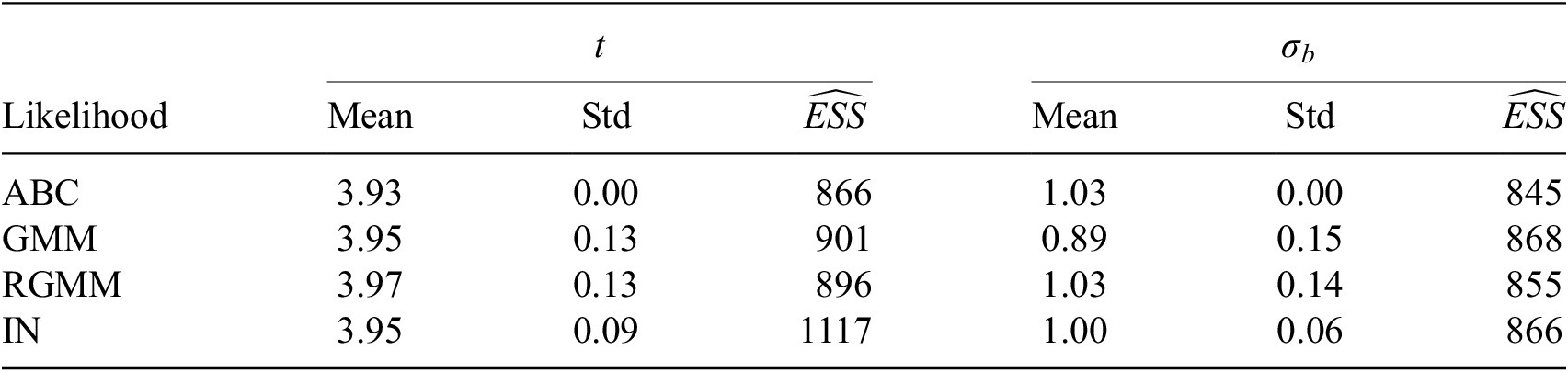
The different likelihood models provide posterior distributions centered around the same values of the unknown parameters. The distribution provided by the ABC likelihood presents significantly less variance than the others. This is due to the fitting of
 $ {\sigma}_b $
being exact up to
$ {\sigma}_b $
being exact up to
 $ \epsilon $
as a difference, while the other likelihoods have larger acceptance probabilities for the values of
$ \epsilon $
as a difference, while the other likelihoods have larger acceptance probabilities for the values of
 $ {\sigma}_b $
. Alternative values for
$ {\sigma}_b $
. Alternative values for
 $ \epsilon $
would have been less restrictive in the fitting of the moments, generating a flatter likelihood distribution that would have led to a wider posterior. There is no significant difference in the convergence speed for this particular dataset. The difference between the means of the parameters and the true generating ones is rooted in the specific realization of the dataset. However, it must be noted that ABC is the only likelihood that does not cover the true generating parameters for any reasonable confidence interval, as it aims to fit exactly the moments of a particular sample dataset.
$ \epsilon $
would have been less restrictive in the fitting of the moments, generating a flatter likelihood distribution that would have led to a wider posterior. There is no significant difference in the convergence speed for this particular dataset. The difference between the means of the parameters and the true generating ones is rooted in the specific realization of the dataset. However, it must be noted that ABC is the only likelihood that does not cover the true generating parameters for any reasonable confidence interval, as it aims to fit exactly the moments of a particular sample dataset.
Four QoI are evaluated for
 $ x=1.0 $
: the output
$ x=1.0 $
: the output
 $ y $
, the mean of the predictive distribution
$ y $
, the mean of the predictive distribution
 $ {\mu}_P^f $
, the standard deviation
$ {\mu}_P^f $
, the standard deviation
 $ {\sigma}_P^f $
and the z-value of
$ {\sigma}_P^f $
and the z-value of
 $ y(1.0) $
. The QoI generally can have physical meaning or simply be indicators of performance. In this case, due to the simplicity of the application, they represent quantities of statistical importance that can be used for an analysis of the fitness of the predictions. In a classical inference problem, these quantities would be deterministic, which would not allow for an analysis of the reliability of the QoIs themselves. The output
$ y(1.0) $
. The QoI generally can have physical meaning or simply be indicators of performance. In this case, due to the simplicity of the application, they represent quantities of statistical importance that can be used for an analysis of the fitness of the predictions. In a classical inference problem, these quantities would be deterministic, which would not allow for an analysis of the reliability of the QoIs themselves. The output
 $ y $
is directly the pushed-forward prediction
$ y $
is directly the pushed-forward prediction
 $ {\boldsymbol{f}}_P=\boldsymbol{f}\left(\boldsymbol{t},{\boldsymbol{\sigma}}_{\boldsymbol{b}},\boldsymbol{x}\right) $
, as described in Section 2.7. The other QoIs are calculated for each sample of the posterior distribution of the parameters. In particular, the z-value
$ {\boldsymbol{f}}_P=\boldsymbol{f}\left(\boldsymbol{t},{\boldsymbol{\sigma}}_{\boldsymbol{b}},\boldsymbol{x}\right) $
, as described in Section 2.7. The other QoIs are calculated for each sample of the posterior distribution of the parameters. In particular, the z-value
 $ \mid Z\mid =\left|\frac{\mu_P^f-y(1.0)}{\sigma_P^f}\right| $
can be used for testing the hypothesis
$ \mid Z\mid =\left|\frac{\mu_P^f-y(1.0)}{\sigma_P^f}\right| $
can be used for testing the hypothesis
 $ {H}_1: $
the value
$ {H}_1: $
the value
 $ y(1.0) $
has not been generated by a normal distribution
$ y(1.0) $
has not been generated by a normal distribution
 $ \mathcal{N}\left({\mu}_P^f,{\sigma}_P^f\right) $
against the null hypothesis
$ \mathcal{N}\left({\mu}_P^f,{\sigma}_P^f\right) $
against the null hypothesis
 $ {H}_0 $
. The critical threshold of
$ {H}_0 $
. The critical threshold of
 $ \mid Z\mid $
for a confidence level of 95% is 1.96, allowing to reject
$ \mid Z\mid $
for a confidence level of 95% is 1.96, allowing to reject
 $ {H}_0 $
if the value of
$ {H}_0 $
if the value of
 $ \mid Z\mid $
is significantly larger. For comparison, the equivalent QoIs obtained with the MAP estimator of
$ \mid Z\mid $
is significantly larger. For comparison, the equivalent QoIs obtained with the MAP estimator of
 $ t $
and
$ t $
and
 $ {\sigma}_b $
are calculated as well. The results are plotted in Figure 4.
$ {\sigma}_b $
are calculated as well. The results are plotted in Figure 4.
Analysis of quantities of interest by propagating the posterior distribution of
 $ t $
and
$ t $
and
 $ {\sigma}_b $
for the simple example.
$ {\sigma}_b $
for the simple example.

The obtained propagated distribution is comparable for all likelihoods, either using an estimator of the posterior or sampling from the distribution. The distributions for
 $ {\mu}_P^f $
and
$ {\mu}_P^f $
and
 $ {\sigma}_P^f $
reflect the same conclusions from the pair plot representation. This is due to the linear nature of the system, which propagates directly the posterior distribution of the parameters, as
$ {\sigma}_P^f $
reflect the same conclusions from the pair plot representation. This is due to the linear nature of the system, which propagates directly the posterior distribution of the parameters, as
 $ t $
controls
$ t $
controls
 $ {\mu}_P^f $
and
$ {\mu}_P^f $
and
 $ {\sigma}_b $
,
$ {\sigma}_b $
,
 $ {\sigma}_P^f $
. The z-values are below 1.96 for all likelihoods, failing to reject
$ {\sigma}_P^f $
. The z-values are below 1.96 for all likelihoods, failing to reject
 $ {H}_0 $
, meaning it is plausible that the data point
$ {H}_0 $
, meaning it is plausible that the data point
 $ y(1.0)=5.04 $
was generated by the corresponding posterior distribution. In comparison, if no inadequacy term had been introduced and the posterior only considered the prescribed noise as a source of variance, the corresponding z-value would have been 104, which allows us to reject
$ y(1.0)=5.04 $
was generated by the corresponding posterior distribution. In comparison, if no inadequacy term had been introduced and the posterior only considered the prescribed noise as a source of variance, the corresponding z-value would have been 104, which allows us to reject
 $ {H}_0 $
, inferring that the data point could not have been generated by the prediction. It is noted that if only the estimators where propagated, it would not be possible to generate distributions for three of the QoI, and the values indicated in Figure 4 as dashed lines would be taken as the predicted ones.
$ {H}_0 $
, inferring that the data point could not have been generated by the prediction. It is noted that if only the estimators where propagated, it would not be possible to generate distributions for three of the QoI, and the values indicated in Figure 4 as dashed lines would be taken as the predicted ones.
3.1.1. Dataset dependency analysis
While the obtained results provide insight into the properties of the different likelihoods for this case, it is necessary to compare them with several datasets generated analogously. The described procedure was repeated for 20 datasets with different random seeds for the data generation. The summary of results is presented in Figure 5.
Box plots for the unknown parameters of the embedded model with different likelihoods. Outliers are indicated as rhomboids. Mean and standard deviation of the posterior distribution after 1000 MCMC evaluations with 10 walkers and 200 burn-in steps for 20 different realizations of the dataset. Mean (top left) and standard deviation (top right) for the slope variable
 $ t $
and mean (bottom left) and standard deviation (bottom right) of the model inadequacy scale parameter
$ t $
and mean (bottom left) and standard deviation (bottom right) of the model inadequacy scale parameter
 $ {\sigma}_b $
. True generating values are indicated as a dot-dashed line in the means.
$ {\sigma}_b $
. True generating values are indicated as a dot-dashed line in the means.

As can be observed, the mean value of
 $ t $
using ABC varies the most from dataset to dataset, with the others being mostly equivalent. Coincidentally, ABC presents the smallest variance in the posterior of
$ t $
using ABC varies the most from dataset to dataset, with the others being mostly equivalent. Coincidentally, ABC presents the smallest variance in the posterior of
 $ t $
, followed by IN, GMM, and RGMM. Due to the limited dataset, ABC tends to overfit to the available points, whose statistics may present a discrepancy from the generating model ones, as ABC aims to fit the moments exactly. When comparing the model form uncertainty results related to
$ t $
, followed by IN, GMM, and RGMM. Due to the limited dataset, ABC tends to overfit to the available points, whose statistics may present a discrepancy from the generating model ones, as ABC aims to fit the moments exactly. When comparing the model form uncertainty results related to
 $ {\sigma}_b $
, the means for RGMM and IN are comparable. The only difference comes from GMM, for which the limited dataset does not hold the assumptions of the predictions sharing the same distribution, which is required for this likelihood. An analysis of the speed of convergence is presented in Figure 6. The ABC likelihood presents a larger variance in the number of MCMC samples to converge, with a significant amount of outliers for the
$ {\sigma}_b $
, the means for RGMM and IN are comparable. The only difference comes from GMM, for which the limited dataset does not hold the assumptions of the predictions sharing the same distribution, which is required for this likelihood. An analysis of the speed of convergence is presented in Figure 6. The ABC likelihood presents a larger variance in the number of MCMC samples to converge, with a significant amount of outliers for the
 $ \hat{ESS} $
of
$ \hat{ESS} $
of
 $ {\sigma}_b $
. Due to the exact matching of the statistical moments, the ABC likelihood may require longer chains in the MCMC algorithm. It must be noted that this can be controlled by the value of the tolerance parameter
$ {\sigma}_b $
. Due to the exact matching of the statistical moments, the ABC likelihood may require longer chains in the MCMC algorithm. It must be noted that this can be controlled by the value of the tolerance parameter
 $ \epsilon $
. The other likelihood models present comparable convergence behavior with each other.
$ \epsilon $
. The other likelihood models present comparable convergence behavior with each other.
Boxplot of required number of MCMC samples until reaching the threshold
 $ \hat{ESS}=837 $
in both variables for the simple example.
$ \hat{ESS}=837 $
in both variables for the simple example.

3.1.2. Noise influence analysis
It has been proven in Section 2 and Appendix B, that the ABC likelihood is very sensitive to the prescribed additive noise
 $ {\sigma}_N $
, and in particular to its misspecification. We repeat the basic experiment, but with 20 different values for the prescribed
$ {\sigma}_N $
, and in particular to its misspecification. We repeat the basic experiment, but with 20 different values for the prescribed
 $ {\sigma}_N $
between 0.001 and 10.0 and the same prior distribution. The posterior predictive results are presented in Figure 7 and the compared influence of the noise in Figure 8.
$ {\sigma}_N $
between 0.001 and 10.0 and the same prior distribution. The posterior predictive results are presented in Figure 7 and the compared influence of the noise in Figure 8.
Posterior prediction comparison for noise value
 $ {\sigma}_N $
of 0.001,
$ {\sigma}_N $
of 0.001,
 $ {e}^{-2} $
and
$ {e}^{-2} $
and
 $ {e}^{0.85} $
, chosen using a logarithmic rule. Dashed lines indicate the interval of
$ {e}^{0.85} $
, chosen using a logarithmic rule. Dashed lines indicate the interval of
 $ {\mu}^f\pm {\sigma}^f $
.
$ {\mu}^f\pm {\sigma}^f $
.

Influence of prescribed noise value
 $ {\sigma}_N $
for the posterior of (a) slope variable
$ {\sigma}_N $
for the posterior of (a) slope variable
 $ t $
and (b) inadequacy scale variable
$ t $
and (b) inadequacy scale variable
 $ {\sigma}_b $
. Dashed lines indicate the interval of
$ {\sigma}_b $
. Dashed lines indicate the interval of
 $ \pm \sigma $
.
$ \pm \sigma $
.

As expected, the ABC likelihood is the most sensitive to noise misspecification, particularly for values of
 $ {\sigma}_N $
exceeding 1.0. When
$ {\sigma}_N $
exceeding 1.0. When
 $ {\sigma}_N<0.01 $
, the prescribed noise underestimates the true generative noise, and the resulting variability is absorbed by the model form uncertainty. However, due to the scale difference, this effect is not visible in the results. For
$ {\sigma}_N<0.01 $
, the prescribed noise underestimates the true generative noise, and the resulting variability is absorbed by the model form uncertainty. However, due to the scale difference, this effect is not visible in the results. For
 $ 0.01<{\sigma}_N $
, the noise is overestimated for at least some data points, reducing the contribution of
$ 0.01<{\sigma}_N $
, the noise is overestimated for at least some data points, reducing the contribution of
 $ {\sigma}_i^f $
to the predictive variance at those locations. Notably, for
$ {\sigma}_i^f $
to the predictive variance at those locations. Notably, for
 $ {\sigma}_N>0.4 $
, the prescribed noise surpasses the variance of the data generator at certain points, leading to significant shifts in the inferred parameters. Once
$ {\sigma}_N>0.4 $
, the prescribed noise surpasses the variance of the data generator at certain points, leading to significant shifts in the inferred parameters. Once
 $ {\sigma}_N>1.0 $
, all data samples exhibit overestimated variance. This overestimation strongly affects the unknown parameter
$ {\sigma}_N>1.0 $
, all data samples exhibit overestimated variance. This overestimation strongly affects the unknown parameter
 $ t $
in ABC, which attempts to match both the mean and variance precisely. Although other likelihoods also degrade in performance as noise increases, their sensitivity is less pronounced than that of ABC. Additionally, for large
$ t $
in ABC, which attempts to match both the mean and variance precisely. Although other likelihoods also degrade in performance as noise increases, their sensitivity is less pronounced than that of ABC. Additionally, for large
 $ {\sigma}_N $
, ABC exhibits irregular behavior due to the emergence of local minima in the likelihood, causing some chains to converge prematurely and introducing numerical instability. In contrast, GMM, RGMM, and especially IN are considerably more robust to noise misspecification. While GMM and RGMM yield estimates of
$ {\sigma}_N $
, ABC exhibits irregular behavior due to the emergence of local minima in the likelihood, causing some chains to converge prematurely and introducing numerical instability. In contrast, GMM, RGMM, and especially IN are considerably more robust to noise misspecification. While GMM and RGMM yield estimates of
 $ t $
that deviate more from the true value (
$ t $
that deviate more from the true value (
 $ t=4.0 $
) than IN, their confidence intervals remain narrow. For IN, the interval widens with increasing noise. It is also worth noting that due to heteroscedasticity in the discrepancy between predictions and observations, stemming from randomness in
$ t=4.0 $
) than IN, their confidence intervals remain narrow. For IN, the interval widens with increasing noise. It is also worth noting that due to heteroscedasticity in the discrepancy between predictions and observations, stemming from randomness in
 $ \theta $
,
$ \theta $
,
 $ {\sigma}_b $
remains nonzero to account for prediction errors not captured by the homoscedastic noise
$ {\sigma}_b $
remains nonzero to account for prediction errors not captured by the homoscedastic noise
 $ {\sigma}_N $
. These effects are particularly pronounced for unrealistically large values of prescribed noise.
$ {\sigma}_N $
. These effects are particularly pronounced for unrealistically large values of prescribed noise.
3.1.3. Offset influence analysis
Another influential factor in the choice of the likelihood formulation is the existence of data points that cannot be replicated by the response function. This can be simulated by including an additive offset
 $ \Delta y $
to the generator as
$ \Delta y $
to the generator as
 $$ y=\theta x+\Delta y+{\varepsilon}_N $$
while keeping the original computational model. This case is relevant, for example, for non-stationary problems that depend on initial conditions, which may introduce such an offset. An offset in the range between 0.0 and 1.0 is tested. The posterior predictive results are presented in Figure 9 and the influence comparison in Figure 10. Increasing offset values lead to higher values for
 $ t $
to try to fit the observed points. At the same time, this leads to the need for larger variances to cover the dataset. This effect is more pronounced in RGMM and IN as the offset impacts in particular values with smaller
$ t $
to try to fit the observed points. At the same time, this leads to the need for larger variances to cover the dataset. This effect is more pronounced in RGMM and IN as the offset impacts in particular values with smaller
 $ {\sigma}_i^f $
that need larger changes in
$ {\sigma}_i^f $
that need larger changes in
 $ t $
and
$ t $
and
 $ {\sigma}_b $
to cover the new dataset, and coincidentally, are those with the largest weight in those likelihood models. Comparing the values for the mean of
$ {\sigma}_b $
to cover the new dataset, and coincidentally, are those with the largest weight in those likelihood models. Comparing the values for the mean of
 $ t $
with offsets of 0.0 and 1.0, it can be observed that IN and RGMM evolve less favorably than GMM with the addition of such an offset, as was expected, since the marginalizing effect is stronger in such likelihood models. For smaller datasets where the individual points have a larger weight, we expect this tendency to be more acute, leading to improvements of RGMM over IN as well, driven by the addition of the second moment fitting.
$ t $
with offsets of 0.0 and 1.0, it can be observed that IN and RGMM evolve less favorably than GMM with the addition of such an offset, as was expected, since the marginalizing effect is stronger in such likelihood models. For smaller datasets where the individual points have a larger weight, we expect this tendency to be more acute, leading to improvements of RGMM over IN as well, driven by the addition of the second moment fitting.
Posterior prediction comparison for offset values of 0.0, 0.5, and 1.0.

Influence of prescribed offset
 $ \Delta y $
for the posterior of (a) slope variable
$ \Delta y $
for the posterior of (a) slope variable
 $ t $
and (b) model inadequacy scale variable
$ t $
and (b) model inadequacy scale variable
 $ {\sigma}_b $
. Dashed lines indicate the interval of
$ {\sigma}_b $
. Dashed lines indicate the interval of
 $ \pm \sigma $
.
$ \pm \sigma $
.

3.1.4. Outlier influence analysis
An alternative situation in which an offset is present is if it only affects a given subset of data points, creating a group of outliers that influence the inference. In this case, Equation 55 is modified to only affect a subset of samples such that
 $$ y=\left\{\begin{array}{ll}\theta x+{\varepsilon}_N& \mathrm{if}\hskip0.32em x\in \left[\mathrm{0.4,}\;\mathrm{0.6}\right)\cup \left(\mathrm{0.7,}\;\mathrm{1.0}\right]\\ {}\theta x-\Delta y+{\varepsilon}_N& \mathrm{if}\hskip0.32em x\in \left[\mathrm{0.6,}\;\mathrm{0.7}\right]\end{array}\right.. $$
The offset ranges from 0.0 to 2.0 in 21 samples. The posterior predictive results are presented in Figure 11 and the comparison in Figure 12.
Posterior prediction comparison for outlier’s offset values of 0.0, −0.5, and −1.0. The zones with outliers are shaded in grey. Dashed lines indicate the interval of
 $ {\mu}^f\pm {\sigma}^f $
.
$ {\mu}^f\pm {\sigma}^f $
.

Influence of outlier data magnitude on the posterior of (a) slope variable
 $ t $
and (b) model inadequacy scale variable
$ t $
and (b) model inadequacy scale variable
 $ {\sigma}_b $
. Dashed lines indicate the interval of
$ {\sigma}_b $
. Dashed lines indicate the interval of
 $ \pm \sigma $
.
$ \pm \sigma $
.

In this case, ABC is the most affected in comparison with the other likelihood models. The outliers can be represented by the predicted response, but the fitting of every point with equal weight provokes larger deviations in ABC. Nevertheless, if the outliers are located at data points with low predicted variance, it is expected that RGMM and IN show a larger influence.
3.2. Application case: transient thermal simulation of reinforced concrete
The second application case consists of a transient thermal 2D simulation of the section of a reinforced concrete cylinder with constant external temperature. Due to symmetry and under the assumption of an infinitely long cylinder, such a system can be modeled as a 2D square section with adiabatic boundary conditions at the top, bottom, and left-hand sides and constant temperature at the right-hand side. Figure 13 shows a schematic representation of the case. The adiabatic conditions represent the periodic nature of the reinforcement for the sides and an isolation layer for the back. The system is reduced from a 3D cube to a 2D section, assuming constant properties in the X direction. The diagrams in Figure 14 represent the generative and forward models for this application case. The objective is to obtain the total cumulative heat
 $ {Q}_{\mathrm{obj}}(t) $
that passes through the middle line of the section at a given time.
$ {Q}_{\mathrm{obj}}(t) $
that passes through the middle line of the section at a given time.
Schematic diagram of the heat example case for a differential slice d
 $ s $
.
$ s $
.

Diagrams of the systems modeled in the thermal example. (a) System with isotropic material properties
 $ {\mathcal{M}}_{\mathrm{con}} $
and (b) system with a band with modified material properties
$ {\mathcal{M}}_{\mathrm{con}} $
and (b) system with a band with modified material properties
 $ {\mathcal{M}}_{\mathrm{rein}} $
that represent a reinforcement bar in that region. The temperature sensors
$ {\mathcal{M}}_{\mathrm{rein}} $
that represent a reinforcement bar in that region. The temperature sensors
 $ {T}_i(t) $
for
$ {T}_i(t) $
for
 $ i=\mathrm{1,2,3,4} $
act as real sensors and are used for updating the material parameters of
$ i=\mathrm{1,2,3,4} $
act as real sensors and are used for updating the material parameters of
 $ {\mathcal{M}}_{\mathrm{con}} $
. The virtual sensor
$ {\mathcal{M}}_{\mathrm{con}} $
. The virtual sensor
 $ {\dot{Q}}_{\mathrm{obj}}(t) $
predicts the heat through the midline of the system obtained by integrating its normal heat flow obtained from the gradient of the temperature field. The quantity of interest
$ {\dot{Q}}_{\mathrm{obj}}(t) $
predicts the heat through the midline of the system obtained by integrating its normal heat flow obtained from the gradient of the temperature field. The quantity of interest
 $ {Q}_{\mathrm{obj}}(t) $
is the cumulative heat through the middle line at a given
$ {Q}_{\mathrm{obj}}(t) $
is the cumulative heat through the middle line at a given
 $ t $
.
$ t $
.

The transient thermal system follows the heat equation for temperature
 $ T $
$ T $
 $$ \rho {c}_p\frac{\partial T}{\partial t}-\nabla \cdot \left(k\nabla T\right)={\dot{q}}_V $$
where
 $ \rho $
is the density of the material,
$ \rho $
is the density of the material,
 $ {c}_p $
its heat capacity,
$ {c}_p $
its heat capacity,
 $ k $
its conductivity, and
$ k $
its conductivity, and
 $ {\dot{q}}_V $
is the volumetric heat flux in the system. There exists a linear relationship between
$ {\dot{q}}_V $
is the volumetric heat flux in the system. There exists a linear relationship between
 $ k $
and
$ k $
and
 $ {c}_p $
for a given
$ {c}_p $
for a given
 $ \rho $
which is the diffusivity
$ \rho $
which is the diffusivity
 $ \alpha =k/\left(\rho {c}_p\right) $
, which requires correcting the heat component as
$ \alpha =k/\left(\rho {c}_p\right) $
, which requires correcting the heat component as
 $ {\dot{q}}_V/\left(\rho {c}_p\right) $
. The heat flux vector field at a given time
$ {\dot{q}}_V/\left(\rho {c}_p\right) $
. The heat flux vector field at a given time
 $ t $
is defined as
$ t $
is defined as
 $$ \dot{\mathbf{q}}(t)=-k\nabla T, $$
where
 $ k $
is calculated for a certain
$ k $
is calculated for a certain
 $ \rho $
,
$ \rho $
,
 $ {c}_p $
, and
$ {c}_p $
, and
 $ \alpha $
, and the heat flux through the midline is obtained by integrating the normal heat flux field over the facet
$ \alpha $
, and the heat flux through the midline is obtained by integrating the normal heat flux field over the facet
 $ S $
as
$ S $
as
 $$ {\dot{Q}}_{\mathrm{obj}}(t)=\int \dot{\mathbf{q}}(t)\cdot \mathbf{n}\hskip0.1em dS. $$
The cumulative heat at time
 $ {t}_n $
is obtained by integrating
$ {t}_n $
is obtained by integrating
 $ {\dot{Q}}_{\mathrm{obj}}(t) $
over time, which in this case will be done using a trapezoidal rule as
$ {\dot{Q}}_{\mathrm{obj}}(t) $
over time, which in this case will be done using a trapezoidal rule as
 $$ {Q}_{\mathrm{obj}}\left({t}_n\right)={\int}_{t_0}^{t_n}{\dot{Q}}_{\mathrm{obj}}(t)\hskip0.1em dt\approx \sum \limits_{i=0}^{n-1}\frac{\Delta {t}_i}{2}\left[{\dot{Q}}_{\mathrm{obj}}\left({t}_i\right)+{\dot{Q}}_{\mathrm{obj}}\left({t}_{i+1}\right)\right], $$
where
 $ {t}_i $
are the discretized time points and
$ {t}_i $
are the discretized time points and
 $ \Delta {t}_i $
is the interval between two consecutive times
$ \Delta {t}_i $
is the interval between two consecutive times
 $ {t}_i $
and
$ {t}_i $
and
 $ {t}_{i+1} $
.
$ {t}_{i+1} $
.
Altogether, the system’s geometry, material properties
 $ \rho $
,
$ \rho $
,
 $ {c}_p $
, and
$ {c}_p $
, and
 $ k $
and its thermal and initial boundary conditions are required to calculate
$ k $
and its thermal and initial boundary conditions are required to calculate
 $ {\dot{Q}}_{\mathrm{obj}}(t) $
. In this case, the squared slab has a length of 0.4 m in each direction, with adiabatic boundary conditions on three sides (
$ {\dot{Q}}_{\mathrm{obj}}(t) $
. In this case, the squared slab has a length of 0.4 m in each direction, with adiabatic boundary conditions on three sides (
 $ \dot{Q}=0 $
W) and fixed external temperature
$ \dot{Q}=0 $
W) and fixed external temperature
 $ {T}_{\mathrm{ext}}=303 $
K. The initial temperature at all points of the system is
$ {T}_{\mathrm{ext}}=303 $
K. The initial temperature at all points of the system is
 $ T\left(t=0\right)=273 $
K and we assume a known density for the concrete of 2300 kg/m
$ T\left(t=0\right)=273 $
K and we assume a known density for the concrete of 2300 kg/m
 $ {}^3 $
. The diffusivity value
$ {}^3 $
. The diffusivity value
 $ \alpha $
determines the thermal behavior and must be estimated from the observations.
$ \alpha $
determines the thermal behavior and must be estimated from the observations.
For the parameter estimation, two material models are implemented: an isotropic one
 $ {\mathcal{M}}_{\mathrm{con}} $
for the forward model and a biphasic one
$ {\mathcal{M}}_{\mathrm{con}} $
for the forward model and a biphasic one
 $ {\mathcal{M}}_{\mathrm{con}}+{\mathcal{M}}_{\mathrm{rein}} $
representing the real reinforced system for the generative model.
$ {\mathcal{M}}_{\mathrm{con}}+{\mathcal{M}}_{\mathrm{rein}} $
representing the real reinforced system for the generative model.
 $ {\mathcal{M}}_{\mathrm{con}} $
is based on the assumption that the whole system shares the same material properties. Therefore,
$ {\mathcal{M}}_{\mathrm{con}} $
is based on the assumption that the whole system shares the same material properties. Therefore,
 $ {\mathcal{M}}_{\mathrm{con}}=\left\{\rho =2300\;\mathrm{kg}/{\mathrm{m}}^3,{c}_p=900\;\mathrm{J}/\left(\mathrm{kg}\cdot \mathrm{K}\right),\alpha \right\} $
with
$ {\mathcal{M}}_{\mathrm{con}}=\left\{\rho =2300\;\mathrm{kg}/{\mathrm{m}}^3,{c}_p=900\;\mathrm{J}/\left(\mathrm{kg}\cdot \mathrm{K}\right),\alpha \right\} $
with
 $ \alpha $
to be inferred. The values of
$ \alpha $
to be inferred. The values of
 $ \rho $
and
$ \rho $
and
 $ {c}_p $
have been chosen to reflect concrete properties at
$ {c}_p $
have been chosen to reflect concrete properties at
 $ T=293 $
K according to EN 1992-1-2:2004 (European Committee for Standardization, 2004). A reference value for the conductivity from these conditions is
$ T=293 $
K according to EN 1992-1-2:2004 (European Committee for Standardization, 2004). A reference value for the conductivity from these conditions is
 $ k=2.0 $
W/(m
$ k=2.0 $
W/(m
 $ \cdot $
K). This simplified model responds to the situation where the location of the reinforcement bars is not known beforehand or their effect on the simulation is disregarded.
$ \cdot $
K). This simplified model responds to the situation where the location of the reinforcement bars is not known beforehand or their effect on the simulation is disregarded.
The biphasic model
 $ {\mathcal{M}}_{\mathrm{con}}^{\ast }+{\mathcal{M}}_{\mathrm{rein}} $
is used to generate the “real” observations required for the parameter estimation. The system is divided into two materials,
$ {\mathcal{M}}_{\mathrm{con}}^{\ast }+{\mathcal{M}}_{\mathrm{rein}} $
is used to generate the “real” observations required for the parameter estimation. The system is divided into two materials,
 $ {\mathcal{M}}_{\mathrm{con}}^{\ast } $
for the concrete and
$ {\mathcal{M}}_{\mathrm{con}}^{\ast } $
for the concrete and
 $ {\mathcal{M}}_{\mathrm{rein}} $
for the reinforcement. The properties for the concrete are taken from EN 1992-1-2:2004 (European Committee for Standardization, 2004) as
$ {\mathcal{M}}_{\mathrm{rein}} $
for the reinforcement. The properties for the concrete are taken from EN 1992-1-2:2004 (European Committee for Standardization, 2004) as
 $ {\mathcal{M}}_{\mathrm{con}}^{\ast }=\left\{\rho =2300\;\mathrm{kg}/{\mathrm{m}}^3,{c}_p=900\;\mathrm{J}/\left(\mathrm{kg}\cdot \mathrm{K}\right),\alpha =9.66\mathrm{e}\hbox{-} 7\;{\mathrm{m}}^2/\mathrm{s}\right\} $
. To obtain
$ {\mathcal{M}}_{\mathrm{con}}^{\ast }=\left\{\rho =2300\;\mathrm{kg}/{\mathrm{m}}^3,{c}_p=900\;\mathrm{J}/\left(\mathrm{kg}\cdot \mathrm{K}\right),\alpha =9.66\mathrm{e}\hbox{-} 7\;{\mathrm{m}}^2/\mathrm{s}\right\} $
. To obtain
 $ {\mathcal{M}}_{\mathrm{rein}} $
, a mix of material properties from the steel of the reinforcement and the concrete part must be considered. The region denoted for
$ {\mathcal{M}}_{\mathrm{rein}} $
, a mix of material properties from the steel of the reinforcement and the concrete part must be considered. The region denoted for
 $ {\mathcal{M}}_{\mathrm{rein}} $
has a height of 0.02 m located between Y=0.16 m and Y=0.18 m, which, assuming the same depth, leads to a total surface perpendicular to the reinforcement of 0.0004 m
$ {\mathcal{M}}_{\mathrm{rein}} $
has a height of 0.02 m located between Y=0.16 m and Y=0.18 m, which, assuming the same depth, leads to a total surface perpendicular to the reinforcement of 0.0004 m
 $ {}^2 $
. Using a standard bar diameter of 12 mm, the fractional volumes for concrete and steel are
$ {}^2 $
. Using a standard bar diameter of 12 mm, the fractional volumes for concrete and steel are
 $$ {f}_{\mathrm{steel}}=\frac{V_{\mathrm{steel}}}{V_{\mathrm{total}}}=\frac{A_{\mathrm{steel}}\cdot L}{A_{\mathrm{total}}\cdot L}=\frac{0.012^2\cdot 0.25\cdot \pi }{0.0004}=0.283 $$
and
 $$ {f}_{\mathrm{concrete}}=1-{f}_{\mathrm{steel}}=0.717. $$
The material parameters
 $ {M}_i $
of
$ {M}_i $
of
 $ {\mathcal{M}}_{\mathrm{rein}} $
are then calculated following a Voigt model as
$ {\mathcal{M}}_{\mathrm{rein}} $
are then calculated following a Voigt model as
 $$ {M}_i={f}_{\mathrm{steel}}{M}_{\mathrm{steel}}+{f}_{\mathrm{concrete}}{M}_{\mathrm{concrete}}, $$
which for
 $ {\mathcal{M}}_{\mathrm{steel}}=\left\{\rho =7850\;\mathrm{kg}/{\mathrm{m}}^3,{c}_p=440\;\mathrm{J}/\left(\mathrm{kg}\cdot \mathrm{K}\right),\alpha =1.56\mathrm{e}\hbox{-} 5\;{\mathrm{m}}^2/\mathrm{s}\right\} $
(obtained from EN 1993-1-2:2005 (European Committee for Standardization, 2005) with
$ {\mathcal{M}}_{\mathrm{steel}}=\left\{\rho =7850\;\mathrm{kg}/{\mathrm{m}}^3,{c}_p=440\;\mathrm{J}/\left(\mathrm{kg}\cdot \mathrm{K}\right),\alpha =1.56\mathrm{e}\hbox{-} 5\;{\mathrm{m}}^2/\mathrm{s}\right\} $
(obtained from EN 1993-1-2:2005 (European Committee for Standardization, 2005) with
 $ k=54.0 $
W/(m
$ k=54.0 $
W/(m
 $ \cdot $
K)) leads to
$ \cdot $
K)) leads to
 $ {\mathcal{M}}_{\mathrm{rein}}=\left\{\rho =3871\;\mathrm{kg}/{\mathrm{m}}^3,{c}_p=770\;\mathrm{J}/\left(\mathrm{kg}\cdot \mathrm{K}\right),\alpha =5.61\mathrm{e}\hbox{-} 6\;{\mathrm{m}}^2/\mathrm{s}\right\} $
with
$ {\mathcal{M}}_{\mathrm{rein}}=\left\{\rho =3871\;\mathrm{kg}/{\mathrm{m}}^3,{c}_p=770\;\mathrm{J}/\left(\mathrm{kg}\cdot \mathrm{K}\right),\alpha =5.61\mathrm{e}\hbox{-} 6\;{\mathrm{m}}^2/\mathrm{s}\right\} $
with
 $ k=16.7 $
W/(m
$ k=16.7 $
W/(m
 $ \cdot $
K). The material properties for the generative model are summarized in Table 3. There is a possible argument to use a Reuss model for some of the material properties, in particular the conductivity
$ \cdot $
K). The material properties for the generative model are summarized in Table 3. There is a possible argument to use a Reuss model for some of the material properties, in particular the conductivity
 $ k $
. The mixed materials with such a model would be obtained as
$ k $
. The mixed materials with such a model would be obtained as
 $$ \frac{1}{M_i}=\frac{f_{\mathrm{steel}}}{M_{\mathrm{steel}}}+\frac{f_{\mathrm{concrete}}}{M_{\mathrm{concrete}}}. $$
However, the use of Voigt’s model provides a better approximation than Reuss’ model for all the studied properties when the heat flow is parallel to the reinforcement (Ben-Amoz, Reference Ben-Amoz1970). More complex formulations are possible, but would only be justified if the direction of the reinforcement were unknown and non-homogeneous.
Material properties used for the generative model of the thermal application case
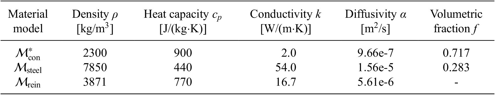
In a real application, it would not be possible to obtain direct measurements of the heat
 $ {\dot{Q}}_{\mathrm{objective}} $
to infer the value of
$ {\dot{Q}}_{\mathrm{objective}} $
to infer the value of
 $ \alpha $
in
$ \alpha $
in
 $ {\mathcal{M}}_{\mathrm{con}} $
. It is more common to have available temperature readings from sensors installed inside or at the surface of the concrete specimen. Four temperature sensors
$ {\mathcal{M}}_{\mathrm{con}} $
. It is more common to have available temperature readings from sensors installed inside or at the surface of the concrete specimen. Four temperature sensors
 $ {T}_i $
for
$ {T}_i $
for
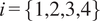 $ i=\left\{\mathrm{1,2,3,4}\right\} $
are placed into the system as in Figure 14 at the coordinates from Table 4. The sensors in the generative model will provide temperature measurements that at a rate of one sample every 5 min for the first 270 min that will be used to infer the unknown parameters. Analogous sensors are defined in the computational model at the same positions. Their observations will be compared during the inference procedure with those collected from the generative model.
$ i=\left\{\mathrm{1,2,3,4}\right\} $
are placed into the system as in Figure 14 at the coordinates from Table 4. The sensors in the generative model will provide temperature measurements that at a rate of one sample every 5 min for the first 270 min that will be used to infer the unknown parameters. Analogous sensors are defined in the computational model at the same positions. Their observations will be compared during the inference procedure with those collected from the generative model.
Sensor coordinates for the thermal application case

Equation 57 is solved over the system to obtain temperature measurements at the sensors. To this end, a finite element (FE) solution is implemented. For simplicity, the geometry is discretized in a regular mesh of
 $ 20\times 20 $
first-order Lagrange elements. The time integration is performed through a backward Euler scheme with 5 min timesteps, which is adequate for the slow evolution of the temperature profile in concrete. The same implementation is used to derive the temperature field to calculate the heat flux through the system. The first 29 min will be used as a transitory regime where the external temperature linearly ramps up starting from 273 K (the same temperature as the system) to 303 K. Afterwards, the external temperature is composed of a constant component of 303 K and an additional component that simulates variable external conditions. This variable component is composed of a short-term noise sampled at every timestep from a distribution
$ 20\times 20 $
first-order Lagrange elements. The time integration is performed through a backward Euler scheme with 5 min timesteps, which is adequate for the slow evolution of the temperature profile in concrete. The same implementation is used to derive the temperature field to calculate the heat flux through the system. The first 29 min will be used as a transitory regime where the external temperature linearly ramps up starting from 273 K (the same temperature as the system) to 303 K. Afterwards, the external temperature is composed of a constant component of 303 K and an additional component that simulates variable external conditions. This variable component is composed of a short-term noise sampled at every timestep from a distribution
 $ \mathcal{N}\left(0\mathrm{K},{\left(1.0\mathrm{K}\right)}^2\right) $
and long-term component that is sampled once every five timesteps from a distribution
$ \mathcal{N}\left(0\mathrm{K},{\left(1.0\mathrm{K}\right)}^2\right) $
and long-term component that is sampled once every five timesteps from a distribution
 $ \mathcal{N}\left(0\mathrm{K},{\left(10.0\mathrm{K}\right)}^2\right) $
and interpolated for the timesteps in between for a smooth transition. Notice that these additional noise components in the temperature are only considered in the data generation, with the isotropic computational model assuming constant external temperature, creating an additional source of model inadequacy. The training and full temperature series are plotted in Figure 15. A comparison of the resolved temperature field at
$ \mathcal{N}\left(0\mathrm{K},{\left(10.0\mathrm{K}\right)}^2\right) $
and interpolated for the timesteps in between for a smooth transition. Notice that these additional noise components in the temperature are only considered in the data generation, with the isotropic computational model assuming constant external temperature, creating an additional source of model inadequacy. The training and full temperature series are plotted in Figure 15. A comparison of the resolved temperature field at
 $ t=20 $
min is shown in Figure 16.
$ t=20 $
min is shown in Figure 16.
External temperature series for the reinforced concrete thermal example. Training series (top) and full temperature series (bottom) for QoI evaluation.

Resolved temperature field a
 $ t=20 $
min. (a) System with isotropic material properties
$ t=20 $
min. (a) System with isotropic material properties
 $ {\mathcal{M}}_{\mathrm{con}} $
and (b) system with a band with modified material properties
$ {\mathcal{M}}_{\mathrm{con}} $
and (b) system with a band with modified material properties
 $ {\mathcal{M}}_{\mathrm{rein}} $
that represent the appearance of a reinforcement bar in that region. The isotropic system presents a uniform temperature gradient from right (
$ {\mathcal{M}}_{\mathrm{rein}} $
that represent the appearance of a reinforcement bar in that region. The isotropic system presents a uniform temperature gradient from right (
 $ T=303 $
K) to left, while the reinforced system presents a faster development of the temperature front at the position of the reinforcement than in the rest of the system.
$ T=303 $
K) to left, while the reinforced system presents a faster development of the temperature front at the position of the reinforcement than in the rest of the system.

The solution of the application consists of two parts: the inference of the material parameters from the temperature measurements and the prediction of the heat flux through the midline section over time. Only thanks to the embedding it is possible to quantify the uncertainty in the heat due to the model inadequacy that steams from the misspecification of the forward model compared to the generative process.
3.2.1. Temperature inference
To infer the diffusivity
 $ \alpha $
of
$ \alpha $
of
 $ {\mathcal{M}}_{\mathrm{con}} $
, an MCMC algorithm is implemented. A training dataset will be used for the parameter estimation and an additional testing dataset will be used for validation. The training dataset
$ {\mathcal{M}}_{\mathrm{con}} $
, an MCMC algorithm is implemented. A training dataset will be used for the parameter estimation and an additional testing dataset will be used for validation. The training dataset
 $ \mathbf{y} $
corresponds to the measurements of
$ \mathbf{y} $
corresponds to the measurements of
 $ T=\left[{T}_1{T}_2{T}_3{T}_4\right] $
between t = 20 min and t = 220 min using the generative model with the reinforcement. The first 20 min have been rejected as they belong to the ramp-up phase and the interest is when the external temperature reaches 303 K. A white noise perturbation with
$ T=\left[{T}_1{T}_2{T}_3{T}_4\right] $
between t = 20 min and t = 220 min using the generative model with the reinforcement. The first 20 min have been rejected as they belong to the ramp-up phase and the interest is when the external temperature reaches 303 K. A white noise perturbation with
 $ {\sigma}_N=0.2 $
K is prescribed at the output. For the testing dataset, the simulation is repeated with a new random seed, gathering measurements between t = 20 min and t = 270 min.The additinola observations in the testing compared to the training are for validation purposes.
$ {\sigma}_N=0.2 $
K is prescribed at the output. For the testing dataset, the simulation is repeated with a new random seed, gathering measurements between t = 20 min and t = 270 min.The additinola observations in the testing compared to the training are for validation purposes.
The embedding for the diffusivity is defined as
 $$ \alpha ={\alpha}_m+{\delta}_b,{\delta}_b\sim \mathcal{N}\left(0,{\left({\sigma}_b\right)}^2\right), $$
where
 $ {\alpha}_m $
and
$ {\alpha}_m $
and
 $ {\sigma}_b $
are the unknown parameters that must be estimated by solving the inverse problem. The prior distributions are
$ {\sigma}_b $
are the unknown parameters that must be estimated by solving the inverse problem. The prior distributions are
 $ \pi \left({\alpha}_m\right)\sim \mathcal{N}\left({10}^{-6},{\left({10}^{-7}\right)}^2\right) $
and
$ \pi \left({\alpha}_m\right)\sim \mathcal{N}\left({10}^{-6},{\left({10}^{-7}\right)}^2\right) $
and
 $ \pi \left({\sigma}_b\right)\sim \mathcal{L}\mathcal{N}\left(-\mathrm{16,0.1}\right) $
(which corresponds to a mean of approximately
$ \pi \left({\sigma}_b\right)\sim \mathcal{L}\mathcal{N}\left(-\mathrm{16,0.1}\right) $
(which corresponds to a mean of approximately
 $ 1.1\mathrm{e}\hbox{-} 7 $
and a standard deviation of approximately
$ 1.1\mathrm{e}\hbox{-} 7 $
and a standard deviation of approximately
 $ 1.1\mathrm{e}\hbox{-} 8 $
). The PCE for computing the forward model with the embedding consist of a Hermite polynomial expansion of degree 2. The noise
$ 1.1\mathrm{e}\hbox{-} 8 $
). The PCE for computing the forward model with the embedding consist of a Hermite polynomial expansion of degree 2. The noise
 $ {\sigma}_N $
is properly specified with a value of 0.2, which is the same used for data generation. The MCMC algorithm is run until convergence with a threshold of
$ {\sigma}_N $
is properly specified with a value of 0.2, which is the same used for data generation. The MCMC algorithm is run until convergence with a threshold of
 $ \hat{ESS}=837 $
after 250 steps of burn-in. The results for the ABC likelihood are presented in Figure 17 and for the other likelihoods in Appendix C (Figures C1–C3). The summarized inference results are presented in Table 5.
$ \hat{ESS}=837 $
after 250 steps of burn-in. The results for the ABC likelihood are presented in Figure 17 and for the other likelihoods in Appendix C (Figures C1–C3). The summarized inference results are presented in Table 5.
Temperature sensors predictions for ABC likelihood. Dashed lines indicate the interval of
 $ {\mu}^f\pm {\sigma}^f $
.
$ {\mu}^f\pm {\sigma}^f $
.

Posterior results for the thermal model and different likelihoods

The results do not present considerable variations between likelihood models for this case. As the noise is well prescribed, the data points with low sensitivity to changes in the parameters are not used for the training and the model can cover reasonably well the inadequacy in the model, all likelihood models produce roughly equivalent results. The posterior response is able to cover the test data points as well as the training ones thanks to the embedding being included in the unknown variable itself. However, the values obtained for
 $ {\alpha}_m $
with mean between
$ {\alpha}_m $
with mean between
 $ 1.27\mathrm{e}\hbox{-} 6 $
and
$ 1.27\mathrm{e}\hbox{-} 6 $
and
 $ 1.32\mathrm{e}\hbox{-} 6 $
are not centered at
$ 1.32\mathrm{e}\hbox{-} 6 $
are not centered at
 $ 9.66\mathrm{e}\hbox{-} 7 $
, concrete’s diffusivity value. This is expected, as there is a model inadequacy between the generative system and the computational model due to the reinforcement bars, that increase the diffusivity. The prescribed noise cannot explain the observed temperature measurements, therefore the embedded model inadequacy is justified. Inferring the noise scale
$ 9.66\mathrm{e}\hbox{-} 7 $
, concrete’s diffusivity value. This is expected, as there is a model inadequacy between the generative system and the computational model due to the reinforcement bars, that increase the diffusivity. The prescribed noise cannot explain the observed temperature measurements, therefore the embedded model inadequacy is justified. Inferring the noise scale
 $ {\sigma}_N $
with an additive model would have allowed to explain the variance in the data points as a perturbation in the output, but would not necessarily be able to explain the variance in the testing range. Classical solutions to this case, such as non-additive or heteroscedastic could achieve better results for the prediction of temperature values, but they would not be transferable to other QoI such as the accumulated heat computations. An analogous situation occurs with the model inadequacy formulated following approaches based on Kennedy and O’Hagan’s framework (Kennedy and O’Hagan, Reference Kennedy and O’Hagan2001), as shown in Andrés Arcones et al. (Reference Andrés Arcones, Weiser, Koutsourelakis and Unger2024).
$ {\sigma}_N $
with an additive model would have allowed to explain the variance in the data points as a perturbation in the output, but would not necessarily be able to explain the variance in the testing range. Classical solutions to this case, such as non-additive or heteroscedastic could achieve better results for the prediction of temperature values, but they would not be transferable to other QoI such as the accumulated heat computations. An analogous situation occurs with the model inadequacy formulated following approaches based on Kennedy and O’Hagan’s framework (Kennedy and O’Hagan, Reference Kennedy and O’Hagan2001), as shown in Andrés Arcones et al. (Reference Andrés Arcones, Weiser, Koutsourelakis and Unger2024).
3.2.2. Heat prediction
Once the posterior distribution of the unknown variables
 $ {\alpha}_m $
and
$ {\alpha}_m $
and
 $ {\sigma}_b $
are estimated by solving the inverse problem, the updated system is used to calculate the cumulative heat through the cross-section. The simulation is run with the full external temperature series of 5000 min, which allows the development of the full thermal profile. Analogously with the simple example, four QoI based on the cumulative heat for
$ {\sigma}_b $
are estimated by solving the inverse problem, the updated system is used to calculate the cumulative heat through the cross-section. The simulation is run with the full external temperature series of 5000 min, which allows the development of the full thermal profile. Analogously with the simple example, four QoI based on the cumulative heat for
 $ t=5000 $
min are evaluated: the output
$ t=5000 $
min are evaluated: the output
 $ {Q}_{\mathrm{obj}}\left(t=5000\;\min \right) $
, the mean of the predictive distribution
$ {Q}_{\mathrm{obj}}\left(t=5000\;\min \right) $
, the mean of the predictive distribution
 $ {\mu}_P^f $
, the standard deviation
$ {\mu}_P^f $
, the standard deviation
 $ {\sigma}_P^f $
and z-value with a confidence of 95% for
$ {\sigma}_P^f $
and z-value with a confidence of 95% for
 $ {Q}_{\mathrm{obj}}\left(t=5000\;\min \right) $
. The predicted response taking the mean values of the posterior distribution and
$ {Q}_{\mathrm{obj}}\left(t=5000\;\min \right) $
. The predicted response taking the mean values of the posterior distribution and
 $ {\hat{\alpha}}_m $
and
$ {\hat{\alpha}}_m $
and
 $ {\hat{\sigma}}_b $
solving equation with them is presented in Figure 18. The propagated posterior distributions of the QoI are plotted in Figure 19. As observed in Figure 18, the posterior distributions generated by the embeddings are able to reliably envelop the real cumulative heat value. The apparent offset is a product of a larger temperature input at the first 300 min in the especific realization of the dataset, as it can be observed in Figure 15. Such is the case due to the similar sources of model inadequacy affecting the QoI calculation and the model updating, i.e. heterogeneity in the material and variations in the external temperature. If the heat simulation presented different sources of model inadequacy, such as larger temperature variations, the predicted distributions may not be able to reflect the true values. Nevertheless, they always provide a more informative assessment on the reliability of the model predictions. In comparison, the prediction when no model inadequacy term is included differs from the true value by more than 10 kJ despite not providing a significant confidence interval, leading to overconfident results.
$ {\hat{\sigma}}_b $
solving equation with them is presented in Figure 18. The propagated posterior distributions of the QoI are plotted in Figure 19. As observed in Figure 18, the posterior distributions generated by the embeddings are able to reliably envelop the real cumulative heat value. The apparent offset is a product of a larger temperature input at the first 300 min in the especific realization of the dataset, as it can be observed in Figure 15. Such is the case due to the similar sources of model inadequacy affecting the QoI calculation and the model updating, i.e. heterogeneity in the material and variations in the external temperature. If the heat simulation presented different sources of model inadequacy, such as larger temperature variations, the predicted distributions may not be able to reflect the true values. Nevertheless, they always provide a more informative assessment on the reliability of the model predictions. In comparison, the prediction when no model inadequacy term is included differs from the true value by more than 10 kJ despite not providing a significant confidence interval, leading to overconfident results.
Temperature heat prediction for each likelihood. Dashed lines indicate the interval of
 $ {\mu}^f\pm {\sigma}^f $
.
$ {\mu}^f\pm {\sigma}^f $
.

Analysis of quantities of interest by propagating the posterior distribution of
 $ \alpha $
and
$ \alpha $
and
 $ {\sigma}_b $
for the thermal example.
$ {\sigma}_b $
for the thermal example.

Analogous conclusions can be extracted from the analysis of the pushed-forward QoIs. While the model without inadequacy term produces a point distribution due to the lack of a noise model for the cumulative heat prediction, the embedded models produce distributions that could have generated the true value of 91338 J. This is reflected in the z-values, where all the sampled pairs of unknown parameters generate distributions that produce z-values significantly smaller than 1.96. Due to its almost zero variance in the posterior distribution, a z-test would not have been reasonable for the model without inadequacy term unless an error model is prescribed. The choice of likelihood does not impact significantly the mean value of the predictions
 $ {\mu}_P^f $
, laying between 82300 and 82550 J. The main difference resides in the value for
$ {\mu}_P^f $
, laying between 82300 and 82550 J. The main difference resides in the value for
 $ {\sigma}_P^f $
and the spread of the distributions for each QoI. In general, ABC produces wider distributions of
$ {\sigma}_P^f $
and the spread of the distributions for each QoI. In general, ABC produces wider distributions of
 $ {Q}_{\mathrm{obj}} $
, with more concentrated values for
$ {Q}_{\mathrm{obj}} $
, with more concentrated values for
 $ {\mu}_P^f $
and
$ {\mu}_P^f $
and
 $ {\sigma}_P^f $
. GMM, RGMM and IN provide comparable results with each other with a more concentrated
$ {\sigma}_P^f $
. GMM, RGMM and IN provide comparable results with each other with a more concentrated
 $ {Q}_{\mathrm{obj}} $
but larger dispersion in the other QoIs. Only slight shifts and deformations in the distributions of the QoI can be observed, tending the global likelihoods to wider ones with more variance.
$ {Q}_{\mathrm{obj}} $
but larger dispersion in the other QoIs. Only slight shifts and deformations in the distributions of the QoI can be observed, tending the global likelihoods to wider ones with more variance.
3.3. Discussion on likelihood selection
As it is clear from the formulation and applications, the likelihood models present substantial differences in their behavior that influence their choice over the others depending on the characteristics of the dataset:
-
• Number of parameters: ABC requires prescribing
$ \gamma $
and
$ \epsilon $
, while GMM and RGMM only require
$ \gamma $
and IN none. As already mentioned, the choice of
$ \epsilon $
is not trivial for datasets with prescribed noise and can largely impact the results. Additionally, the choice of
$ \gamma $
corresponds to previous beliefs on the expected predicted distribution. In particular, a value of
$ \gamma =\sqrt{\frac{\pi }{2}} $
is expected for ABC and
$ \gamma =1.0 $
for the others. The difference in the value of choice for
$ \gamma $
steams from the formulation of the matching of the variance, which induces a half-normal distribution as discussed in Section 2.5.2, while the others do not. -
• Precision specification: As already mentioned and studied in Sargsyan et al. (Reference Sargsyan, Najm and Ghanem2015), the posterior distribution of ABC depends on the specification of the precision parameter
$ \epsilon $
. As the objective is doing a perfect matching of the moments,
$ \epsilon $
is required to be as small as possible. However, it is necessary that
$ \epsilon >0 $
, for numerical stability.In particular,
$ \epsilon $
is usually chosen such that
$ {\epsilon}^2 $
is not under machine precision, e.g.
$ \epsilon ={10}^{-6} $
assuming a machine precision of
$ {10}^{-12} $
. Larger values of
$ \epsilon $
result in an artificially inflated posterior, despite potentially reducing the sensitivity of ABC to the misspecification of noise by relaxing the matching condition. Therefore, higher arbitrary values of
$ \epsilon $
have no real fundament. Using the noise variance in the residuals mitigates the perfect matching of the mean, but using
$ \epsilon $
is unavoidable unless higher order moments are introduced. Contrarily, the respective variances in GMM, RGMM and IN act naturally as a weight on the precision required in the residuals, penalizing higher values of the variance and avoiding the perfect matching. -
• Noise misspecification: As shown in Appendix B, ABC is very sensitive to the specification of the noise amplitude, which can mislead the parameter updating procedure to values of
$ \boldsymbol{\theta} $
further from the expected ones. The misspecification of the prescribed noise generally leads to larger acceptance ratios and wider posterior distribution of
$ \boldsymbol{\theta} $
for GMM, RGMM and IN. -
• Assumptions of normality: The four likelihoods considered suppose different distributions of the residuals while still keeping the assumption of normality. ABC fits exactly the moments under the consideration of Gaussian noise. GMM impose the condition that all the residuals are characterized by the same mixture model, which may not be reasonable. RGMM assume that the relative errors between observations and predicted distribution follow such a common standardized mixture model instead. Finally, IN assumes independent normal distributions for each observation. Depending on the application case, some of these assumptions may not hold. An heteroscedasticity in the noise model can be incorporated in all the likelihoods with minimal modifications, while the assumptions of additive Gaussian noise and Gaussian output require extensive reformulations, specially for IN, GMM, and RGMM. ABC can be adapted to those situations with the current formulation as long as the normal error model for the statistical moments still holds.
-
• Inferred posterior distribution: By construction, ABC aims to match the statistical moments exactly up to a tolerance
$ \epsilon $
, which will lead to narrow inferred posterior distributions of the parameters
$ \boldsymbol{\theta} $
for acceptable values of
$ \epsilon $
compared to GMM, RGMM and IN. In particular, larger predicted variances imply more samples needed for the convergence of the chain (Schälte and Hasenauer, Reference Schälte and Hasenauer2020). Additionally, the formulation of
$ {\mathcal{L}}_2\left(\boldsymbol{\theta} \right) $
for GMM and RGMM produces a flatter likelihood function in the direction of the variance-governing parameters, which further hinders the convergence for those parameters. -
• Observations out of the predictive range: If the observations cannot be replicated by the computational model independently of the choice in the parameters, then embedded approaches lead to suboptimal results. RGMM and IN are expected to be the most impacted if those values are at points with low predictive variance. However, the regularizing effect of considering the whole dataset in RGMM and GMM for the goodness of fit instead of fitting every point, as in IN or ABC, should reduce the impact of these observations if they are not predominant in the dataset.
-
• Fit to exact observations: As pointed out in Sargsyan et al. (Reference Sargsyan, Najm and Ghanem2015), marginalizing formulations such as IN would lead to wrong results if
$ {\sigma}_i^f $
is significantly smaller for a given observation
$ i $
than for the others. In those cases, such observation will be overfitted by reducing the residual to the minimum to the detriment of the other observation points with larger variances. The presence of a prescribed noise reduces this effect in IN, GMM and RGMM likelihoods, as all observations will have at least variance
$ {\sigma}_N $
. For an analysis on this phenomena, refer to Sargsyan et al. (Reference Sargsyan, Najm and Ghanem2015).


4. Conclusions
This paper has introduced several significant advances in the implementation of embedded model inadequacy approaches for quantifying model uncertainties. First, a more interpretable embedding representation was developed as an alternative to the one presented by Sargsyan et al. (Reference Sargsyan, Huan and Najm2019). Although this approach requires specifying a distribution for the model form uncertainty, it reduces the dimensionality of the polynomial chaos expansion (PCE) needed to describe the embedding and improves the separation between fitting the embedding’s PCE and inferring the model parameters. Next, it was demonstrated that the Approximate Bayesian Computation (ABC) likelihood formulation, commonly used to update model parameters with an embedded model inadequacy, is highly sensitive to the prescribed measurement noise and requires careful selection of the parameters
 $ \gamma $
and
$ \gamma $
and
 $ \epsilon $
. One of the main contributions of this work is the explicit treatment and analysis of measurement noise, which had previously been mentioned in past studies but not thoroughly examined. To address this, the ABC likelihood was extended to properly account for measurement noise and accurately quantify predictive variance by imposing
$ \epsilon $
. One of the main contributions of this work is the explicit treatment and analysis of measurement noise, which had previously been mentioned in past studies but not thoroughly examined. To address this, the ABC likelihood was extended to properly account for measurement noise and accurately quantify predictive variance by imposing
 $ \gamma =\sqrt{\pi /2} $
. Additionally, two alternative likelihood formulations, global moment-matching (GMM) and relative global moment-matching (RGMM), were proposed to mitigate sensitivity issues. These formulations were analyzed and compared against the modified ABC likelihood and the independent normal noise formulation using a simple linear and a complex transient thermal example. Finally, a key contribution of this paper is the analysis of how the choice of likelihood influences the propagation of uncertainties, quantified through the embedding approach, to the quantities of interest (QoIs) computed using the updated model and parameters.
$ \gamma =\sqrt{\pi /2} $
. Additionally, two alternative likelihood formulations, global moment-matching (GMM) and relative global moment-matching (RGMM), were proposed to mitigate sensitivity issues. These formulations were analyzed and compared against the modified ABC likelihood and the independent normal noise formulation using a simple linear and a complex transient thermal example. Finally, a key contribution of this paper is the analysis of how the choice of likelihood influences the propagation of uncertainties, quantified through the embedding approach, to the quantities of interest (QoIs) computed using the updated model and parameters.
The inclusion of the embedded model inadequacy term enables the quantification of uncertainty arising during parameter updating due to modeling assumptions, potentially capturing the full range of uncertainties in the measured observations. By introducing the embedding model inadequacy term as a stochastic extension of the unknown parameters, the proposed formulation allows for straightforward propagation of these uncertainties to other predicted QoIs that depend on the same model parameters. However, as shown in this work, the prescribed measurement noise critically influences the selection of the appropriate likelihood formulation and affects the convergence of the Bayesian updating process when an embedding is used. In particular, ABC likelihoods have been identified as the most sensitive to poor noise prescriptions within the embedded model form uncertainty framework. Additionally, the embedded model inadequacy formulation limits predictions to the range of responses that the model is capable of producing. As a result, discrepancies that cannot be explained by changes in the model parameters, such as offsets or outlier values, can skew the inferred parameters. The ABC likelihood formulation tends to be more sensitive to outliers, while RGMM and IN are more impacted by offsets or outliers near values with low variance. GMM and RGMM, on the other hand, are reliable only if the assumption of the existence of a common mixture model in the residuals is valid. Identifying which of these effects are present during model updating is not always possible and often depends on data analysis or practitioner experience. However, selecting the right likelihood function is crucial in certain cases. Regardless of the chosen likelihood formulation, the inclusion of embedded model inadequacy improves predictive posterior distributions, allowing for more informed decision-making, albeit at the cost of increased computational effort during the update phase. While hierarchical Bayesian approaches can produce comparable results when the conditional distributions of the hierarchical formulation are known, a thorough comparison between these methodologies is left for future work.
One of the key strengths of this methodology is its ability to propagate the uncertainty captured by the embedded model inadequacy. This paper has demonstrated how propagating the full posterior distribution of the unknown parameters through QoI calculations provides insights that are not possible with point estimates or model inadequacy-free formulations. Generating distributions for the statistical moments of the predicted QoI enables the use of inference techniques for a more robust analysis of the results. Moreover, the interpretable embedding formulation proposed here allows the propagation of uncertainties related only to specific parameters that influence the QoI being calculated. Nevertheless, when multiple parameters are inferred alongside an associated model form uncertainty, it is likely that their inadequacy terms will be correlated. Implementing and propagating such correlation structures to QoIs where only certain parameters are relevant remains as future work.
While the numerical examples presented in this study involve relatively simple probabilistic structures, they were deliberately selected to isolate and clearly illustrate the methodological contributions and the effects of measurement noise, likelihood formulation, and embedding representation. The proposed approach is not inherently limited to unimodal or low-dimensional distributions; however, its performance for highly complex, multimodal, or non-Gaussian priors has not been explicitly demonstrated here. In such cases, the variance introduced by the embedding may encompass several of the modes, effectively merging distinct peaks into a single broad region of uncertainty. This blending effect can obscure the identification of separate modes and lead to an interpretation of multimodality as merely an increase in overall variance.
Careful selection of the embedding structure and potential modifications to the likelihood formulation could help mitigate these issues, though such strategies typically require some degree of prior knowledge about the underlying distribution. In particular, multi-modal summary statistics or histogram-based distances could be integrated in the likelihood formulations in case that multi-modality is expected. This limitation delineates the current scope of applicability and highlights an important direction for future research. Additionally, it is important to note that the examples presented in this work involve a relatively low-dimensional set of parameters, chosen to allow a clear interpretation of the effects of measurement noise and likelihood selection. Extending the proposed formulation to higher-dimensional parameter spaces represents a natural next step. In many engineering applications, the parameters to be inferred are numerous and may be affected by multiple, potentially interacting sources of bias. Accounting for these multiple discrepancy sources within the embedding would require strategies that ensure the separability and identifiability of the variance contributions associated with each parameter group. Such separability is essential to correctly attribute uncertainties and to reliably propagate them to derived QoIs. Addressing these challenges will be key for applying embedded model inadequacy approaches to complex, real-world systems. Introduction of latent-space approaches such as in Lee et al. (Reference Lee, Yaoyama, Kitahara and Itoi2025) present promising alternatives for dealing with such high-dimensional cases.
In conclusion, the advances presented in this paper represent a significant step toward more effective quantification and propagation of uncertainties in model parameters through embedded model inadequacy approaches. One of the main contributions of this work is the explicit consideration and analysis of measurement noise, which had been previously acknowledged in past methods but never thoroughly examined in terms of its impact on the model updating process. Future work should focus on further validating this methodology by applying it to real measurement data from sensors to assess its practical applicability. Additionally, extending the current approach to hierarchical Bayesian formulations and exploring the propagation of correlated inadequacy terms to various QoIs are important avenues for continued research. These developments promise to enhance the robustness and reliability of uncertainty quantification in complex models.
Data availability statement
The data that support the findings of this study are available in https://doi.org/10.5281/zenodo.15720780 ([dataset] Andres Arconés, Reference Andres Arconés2025). The methodology implemented in this article is available in the software package probeye ([dataset] BAMResearch, 2024), available in the GitHub repository https://github.com/BAMresearch/probeye.
Acknowledgements
The authors made use of ChatGPT to assist with the drafting of this article for the improvement of text clarity and grammar. GPT-4o was accessed from https://chatgpt.com/ and used without modification on 05/03/2025. GPT-5 was used without modification on 27/10/2025 for the improvement of text clarity and grammar during the review process.
Author contribution
Conceptualization: M.W., P.-S.K., J.F.U.; Methodology: D.A.A.; Software: D.A.A.; Data curation: D.A.A.; Data visualization: D.A.A.; Writing original draft: D.A.A.; Supervision: M.W., P.-S.K., J.F.U.; Review and editing: M.W., P.-S.K., J.F.U. All authors approved the final submitted draft.
Funding statement
This research was supported by the German Research Foundation (DFG) in the special focus program SPP 2388/1 “Hundert plus – Verlängerung der Lebensdauer komplexer Baustrukturen durch intelligente Digitalisierung” (Hundred Plus - Extending the service life of complex building structures through intelligent digitalisation) in the subproject C07: Data driven model adaptation for identification of digital twins of bridges.
Competing interests
The authors declare none.
Ethical standard
The research meets all ethical guidelines, including adherence to the legal requirements of the study country.
A. Monte Carlo-Markov Chain stopping criteria
In this paper, the MCMC sampler based on ensembles of chains implemented in emcee (Foreman-Mackey et al., Reference Foreman-Mackey, Hogg, Lang and Goodman2013) is used for the Bayesian updating framework. In the chosen implementation, a stretch move as defined in Goodman and Weare (Reference Goodman and Weare2010) proposes the new samples for the next iteration of the MCMC algorithm based on the current values of the ensemble of chains. The chains in a given ensemble are therefore not independent. This correlation invalidates the use of those convergence criteria that are base on the independence of the chains such as Gelman-Rubin’s
 $ \hat{R} $
metric (Gelman and Rubin, Reference Gelman and Rubin1992; Vats and Knudson, Reference Vats and Knudson2021). Alternatively, the integrated autocorrelation time
$ \hat{R} $
metric (Gelman and Rubin, Reference Gelman and Rubin1992; Vats and Knudson, Reference Vats and Knudson2021). Alternatively, the integrated autocorrelation time
 $ {\tau}_{\infty } $
(Sokal, Reference Sokal, DeWitt-Morette, Cartier and Folacci1997) quantifies how long it takes for the values in a chain or ensemble to become effectively uncorrelated with one another and is in practice a metric of the quality of the ensemble that does not require independence of the chains. A stopping criteria based on the effective sample size
$ {\tau}_{\infty } $
(Sokal, Reference Sokal, DeWitt-Morette, Cartier and Folacci1997) quantifies how long it takes for the values in a chain or ensemble to become effectively uncorrelated with one another and is in practice a metric of the quality of the ensemble that does not require independence of the chains. A stopping criteria based on the effective sample size
 $ ESS $
obtained from
$ ESS $
obtained from
 $ {\tau}_{\infty } $
is imposed on the MCMC algorithm to determine the number of iterations that must be evaluated.
$ {\tau}_{\infty } $
is imposed on the MCMC algorithm to determine the number of iterations that must be evaluated.
First, an objective
 $ ESS $
threshold must be define to determine when the chain is converged. Following Vats et al. (Reference Vats, Flegal and Jones2019), an estimated
$ ESS $
threshold must be define to determine when the chain is converged. Following Vats et al. (Reference Vats, Flegal and Jones2019), an estimated
 $ \hat{ESS} $
such that
$ \hat{ESS} $
such that
 $$ \hat{ESS}\ge {W}_{p,\alpha, \epsilon } $$
is calculated a priori. The value
 $ {W}_{p,\alpha, \epsilon } $
depends only on the dimensionality of the problem
$ {W}_{p,\alpha, \epsilon } $
depends only on the dimensionality of the problem
 $ p $
, the level of confidence
$ p $
, the level of confidence
 $ \alpha $
of the considered regions and the desired precision
$ \alpha $
of the considered regions and the desired precision
 $ \epsilon $
. For large samples, i.e. sufficiently long chains, Vats et al. (Reference Vats, Flegal and Jones2019) prove that a good approximation for
$ \epsilon $
. For large samples, i.e. sufficiently long chains, Vats et al. (Reference Vats, Flegal and Jones2019) prove that a good approximation for
 $ {W}_{p,\alpha, \epsilon } $
is
$ {W}_{p,\alpha, \epsilon } $
is
 $$ \hat{ESS}\ge {W}_{p,\alpha, \epsilon }=\frac{2^{2/p}\pi }{{\left(p\Gamma \left(p/2\right)\right)}^{2/p}}\frac{\chi_{1-\alpha, p}^2}{\epsilon^2}. $$
Additionally, a maximum number of iterations steps
 $ {n}_{\mathrm{max}} $
is established. Therefore, the MCMC algorithm will be continued while, for a given iteration
$ {n}_{\mathrm{max}} $
is established. Therefore, the MCMC algorithm will be continued while, for a given iteration
 $ i $
,
$ i $
,
 $$ {ESS}_i<\frac{2^{2/p}\pi }{{\left(p\Gamma \left(p/2\right)\right)}^{2/p}}\frac{\chi_{1-\alpha, p}^2}{\epsilon^2}\hskip0.5em \mathrm{and}\hskip0.5em i<{n}_{\mathrm{max}}. $$
The effective sample size
 $ {ESS}_i $
is directly related with
$ {ESS}_i $
is directly related with
 $ {\tau}_{\infty } $
at iteration
$ {\tau}_{\infty } $
at iteration
 $ i $
as
$ i $
as
 $$ {ESS}_i=\frac{n_im}{\tau_{\infty }}, $$
where
 $ {n}_i $
is the number of steps at iteration
$ {n}_i $
is the number of steps at iteration
 $ i $
and
$ i $
and
 $ m $
is the number of walkers, i.e. chains in the ensemble. In practice,
$ m $
is the number of walkers, i.e. chains in the ensemble. In practice,
 $ {\tau}_{\infty } $
is approximated by an estimation following the implementation described in Sokal (Reference Sokal, DeWitt-Morette, Cartier and Folacci1997). To avoid excessive computations,
$ {\tau}_{\infty } $
is approximated by an estimation following the implementation described in Sokal (Reference Sokal, DeWitt-Morette, Cartier and Folacci1997). To avoid excessive computations,
 $ {ESS}_i $
is not calculated after every sample of the MCMC algorithm but after a batch of iterations with predefined size have been evaluated. The MCMC will be stopped when the thresholds of Equation A3 are exceeded for the chains of each unknown parameter
$ {ESS}_i $
is not calculated after every sample of the MCMC algorithm but after a batch of iterations with predefined size have been evaluated. The MCMC will be stopped when the thresholds of Equation A3 are exceeded for the chains of each unknown parameter
 $ \theta $
that is being sampled. Convergence plots for the simple case of Section 3.1 are presented in Figure A1, where the stopping criteria has been chosen following the procedure previously described.
$ \theta $
that is being sampled. Convergence plots for the simple case of Section 3.1 are presented in Figure A1, where the stopping criteria has been chosen following the procedure previously described.
Estimated sample size (ESS) for the simple example over the MCMC iterations for simple linear application case.

B. Moment-matching likelihood behavior with measurement noise
Let
 $ \left({A}_i\right) $
denote the residual at observation
$ \left({A}_i\right) $
denote the residual at observation
 $ i $
, defined as
$ i $
, defined as
 $ {A}_i=\left|{\mu}_i^f-{y}_i\right| $
, and let
$ {A}_i=\left|{\mu}_i^f-{y}_i\right| $
, and let
 $ \left({B}_i\right) $
denote the total standard deviation of the model,
$ \left({B}_i\right) $
denote the total standard deviation of the model,
 $ {B}_i=\sqrt{{\left({\sigma}_N\right)}^2+{\left({\sigma}_i^f\right)}^2} $
. The quantities
$ {B}_i=\sqrt{{\left({\sigma}_N\right)}^2+{\left({\sigma}_i^f\right)}^2} $
. The quantities
 $ {A}_i $
and
$ {A}_i $
and
 $ {B}_i $
are independent, since
$ {B}_i $
are independent, since
 $ {A}_i $
depends on the unknown model parameters, while
$ {A}_i $
depends on the unknown model parameters, while
 $ {B}_i $
depends on the auxiliary parameters introduced through the embedded model inadequacy. Then, the noisy moment-matching likelihood from Equation 24, expressed in logarithmic form, is
$ {B}_i $
depends on the auxiliary parameters introduced through the embedded model inadequacy. Then, the noisy moment-matching likelihood from Equation 24, expressed in logarithmic form, is
 $$ \log \mathcal{L}\left(\boldsymbol{\theta} \right)=-\frac{n_y}{2}\log \left(2\pi {\epsilon}^2{\left({\sigma}_N\right)}^2\right)\sum \limits_{i=1}^{n_y}\left[\frac{{\left({A}_i\right)}^2}{2{\left({\sigma}_N\right)}^2}+\frac{{\left({B}_i-\gamma {A}_i\right)}^2}{2{\epsilon}^2}\right]. $$
The objective is to investigate how changes in
 $ {A}_i $
(the residuals) and
$ {A}_i $
(the residuals) and
 $ {B}_i $
(the total deviations) affect the log-likelihood. By analyzing the signs and magnitudes of its first and second derivatives, we can determine how the optimization process will tend to adjust the model residuals and predicted uncertainties, and where potential optima occur.
$ {B}_i $
(the total deviations) affect the log-likelihood. By analyzing the signs and magnitudes of its first and second derivatives, we can determine how the optimization process will tend to adjust the model residuals and predicted uncertainties, and where potential optima occur.
Differentiating the log-likelihood with respect to each residual
 $ {A}_i $
gives
$ {A}_i $
gives
 $$ \frac{c\partial \log \mathcal{L}}{\partial {A}_i}=-\frac{A_i}{{\left({\sigma}_N\right)}^2}+\frac{\gamma \left({B}_i-\gamma {A}_i\right)}{\epsilon^2}=-\left(\frac{1}{{\left({\sigma}_N\right)}^2}+\frac{\gamma^2}{\epsilon^2}\right){A}_i+\frac{\gamma }{\epsilon^2}{B}_i, $$
where
 $ c=\frac{n_y}{2}\log \left(2\pi {\epsilon}^2{\left({\sigma}_N\right)}^2\right) $
. Analogously, differentiation with respect to the total deviation
$ c=\frac{n_y}{2}\log \left(2\pi {\epsilon}^2{\left({\sigma}_N\right)}^2\right) $
. Analogously, differentiation with respect to the total deviation
 $ {B}_i $
yields
$ {B}_i $
yields
 $$ \frac{c\partial \log \mathcal{L}}{\partial {B}_i}=-\frac{B_i-\gamma {A}_i}{\epsilon^2}=\frac{\gamma {A}_i-{B}_i}{\epsilon^2}. $$
These derivatives are defined independently for each observation
 $ i $
, reflecting the separable structure of the log-likelihood. For interpretation, it is convenient to consider the mean derivatives over all observations:
$ i $
, reflecting the separable structure of the log-likelihood. For interpretation, it is convenient to consider the mean derivatives over all observations:
 $$ \frac{c}{n_y}\sum \limits_{i=1}^{n_y}\frac{\partial \log \mathcal{L}}{\partial {A}_i}=-\left(\frac{1}{{\left({\sigma}_N\right)}^2}+\frac{\gamma^2}{\epsilon^2}\right)\overline{A}+\frac{\gamma }{\epsilon^2}\overline{B},\hskip2em \frac{c}{n_y}\sum \limits_{i=1}^{n_y}\frac{\partial \log \mathcal{L}}{\partial {B}_i}=\frac{\gamma }{\epsilon^2}\overline{A}-\frac{1}{\epsilon^2}\overline{B}, $$
where
 $ \overline{A} $
and
$ \overline{A} $
and
 $ \overline{B} $
are the sample means of
$ \overline{B} $
are the sample means of
 $ {A}_i $
and
$ {A}_i $
and
 $ {B}_i $
, respectively. A positive mean derivative with respect to
$ {B}_i $
, respectively. A positive mean derivative with respect to
 $ {A}_i $
implies that increasing the residuals raises the likelihood, suggesting that the optimizer would favor poorer mean-value fits. Conversely, a negative derivative indicates a tendency toward smaller residuals and a better mean-value fit. Similarly, a positive derivative with respect to
$ {A}_i $
implies that increasing the residuals raises the likelihood, suggesting that the optimizer would favor poorer mean-value fits. Conversely, a negative derivative indicates a tendency toward smaller residuals and a better mean-value fit. Similarly, a positive derivative with respect to
 $ {B}_i $
favors higher predicted model-form uncertainty, while a negative value promotes reducing it.
$ {B}_i $
favors higher predicted model-form uncertainty, while a negative value promotes reducing it.
Because the likelihood is separable across observations, the Hessian matrix is block-diagonal, each block corresponding to one observation pair
 $ \left({A}_i,{B}_i\right) $
. For each
$ \left({A}_i,{B}_i\right) $
. For each
 $ i $
:
$ i $
:
 $$ \frac{c{\partial}^2\log \mathcal{L}}{{\left(\partial {A}_i\right)}^2}=-\left(\frac{1}{{\left({\sigma}_N\right)}^2}+\frac{\gamma^2}{\epsilon^2}\right),\hskip2em \frac{c{\partial}^2\log \mathcal{L}}{{\left(\partial {B}_i\right)}^2}=-\frac{1}{\epsilon^2},\hskip2em \frac{c{\partial}^2\log \mathcal{L}}{\partial {A}_i\partial {B}_i}=\frac{c{\partial}^2\log \mathcal{L}}{\partial {B}_i\partial {A}_i}=\frac{\gamma }{\epsilon^2}. $$
The corresponding
 $ 2\times 2 $
Hessian block for observation
$ 2\times 2 $
Hessian block for observation
 $ i $
is
$ i $
is
 $$ {\mathbf{H}}_i=c\left(\begin{array}{cc}-\left(\frac{1}{{\left({\sigma}_N\right)}^2}+\frac{\gamma^2}{\epsilon^2}\right)& \frac{\gamma }{\epsilon^2}\\ {}\frac{\gamma }{\epsilon^2}& -\frac{1}{\epsilon^2}\end{array}\right), $$
and its determinant and trace are
 $$ \det \left({\mathbf{H}}_i\right)=\frac{c^2}{\epsilon^2{\left({\sigma}_N\right)}^2}>0,\hskip2em \mathrm{tr}\left({\mathbf{H}}_i\right)=-c\left(\frac{1}{{\left({\sigma}_N\right)}^2}+\frac{\gamma^2+1}{\epsilon^2}\right)<0. $$
Hence, each block is negative definite, and so is the full Hessian, whose determinant is
 $$ \det \left(\mathbf{H}\right)={c}^2{\left(\frac{1}{\epsilon^2{\left({\sigma}_N\right)}^2}\right)}^{n_y}>0. $$
Therefore, the log-likelihood is globally concave with respect to
 $ {\left\{{A}_i,{B}_i\right\}}_{i=1}^{n_y} $
, and all stationary points correspond to local maxima. Taking the average form of the gradients,
$ {\left\{{A}_i,{B}_i\right\}}_{i=1}^{n_y} $
, and all stationary points correspond to local maxima. Taking the average form of the gradients,
 $$ \frac{c\partial \log \mathcal{L}}{\partial \overline{A}}>0\iff -\left(\frac{1}{{\left({\sigma}_N\right)}^2}+\frac{\gamma^2}{\epsilon^2}\right)\overline{A}+\frac{\gamma }{\epsilon^2}\overline{B}>0,\hskip2em \frac{c\partial \log \mathcal{L}}{\partial \overline{B}}>0\iff \frac{\gamma }{\epsilon^2}\overline{A}-\frac{1}{\epsilon^2}\overline{B}>0. $$
These expressions describe how the mean residuals
 $ \overline{A} $
and mean predicted deviations
$ \overline{A} $
and mean predicted deviations
 $ \overline{B} $
evolve during optimization. They form the basis for the behavioral classification summarized in Table B1. For the likelihood form given by Equation 19, equivalent results follow by setting
$ \overline{B} $
evolve during optimization. They form the basis for the behavioral classification summarized in Table B1. For the likelihood form given by Equation 19, equivalent results follow by setting
 $ {\left({\sigma}_N\right)}^2={\epsilon}^2 $
.
$ {\left({\sigma}_N\right)}^2={\epsilon}^2 $
.
Cases for moment-matching log-likelihood behavior under noise
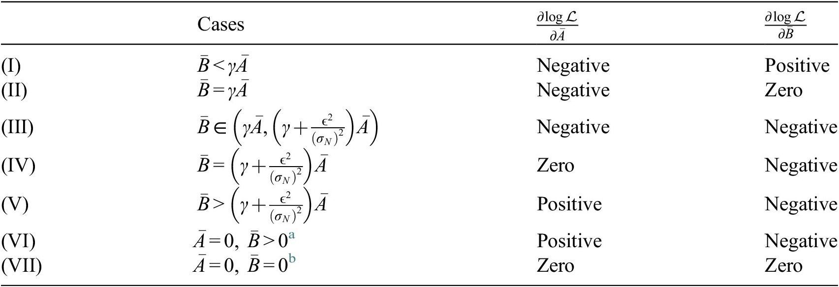
The seven cases summarized in Table B1 describe the qualitative behavior of the noisy moment-matching log-likelihood depending on the relationship between the mean residual
 $ \overline{A} $
and the mean predicted deviation
$ \overline{A} $
and the mean predicted deviation
 $ \overline{B} $
. Each case reflects a characteristic direction of the optimization process in terms of how the model balances residual reduction and predicted variance adjustment. The following interpretations correspond to the derivative signs in each case.
$ \overline{B} $
. Each case reflects a characteristic direction of the optimization process in terms of how the model balances residual reduction and predicted variance adjustment. The following interpretations correspond to the derivative signs in each case.
-
1. Case (I): This case arises when the variance predicted by the model is insufficient to cover the observed residuals (
$ \overline{B}<\gamma \overline{A} $
). The optimization tends to increase the predicted variance while reducing the residuals, moving toward better coverage of the data. This situation typically occurs when the model predictions are inaccurate or the observational noise is underestimated. -
2. Case (II): Here, the model predicts on average the correct level of variance as prescribed by the formulation (
$ \overline{B}=\gamma \overline{A} $
), but the residuals are still larger than ideal. The optimization, therefore, continues to decrease the residuals while maintaining the variance balance. -
3. Case (III): In this range, the model predicts a variance larger than necessary to explain the observations (
$ \overline{B}>\gamma \overline{A} $
but smaller than
$ \left(\gamma +{\epsilon}^2/{\left({\sigma}_N\right)}^2\right)\overline{A} $
). Both derivatives are negative, indicating a joint tendency to reduce both the residual and the predicted variance. When the noise level is fixed, further reduction of the total variance may not be feasible. -
4. Case (IV): This case represents a condition where the residual fitting is optimal under the noisy moment-matching formulation. The equality
$ \overline{B}=\left(\gamma +{\epsilon}^2/{\left({\sigma}_N\right)}^2\right)\overline{A} $
defines the upper bound of the admissible region. In the limit
$ \epsilon \to 0 $
, this condition approaches
$ \overline{B}=\gamma \overline{A} $
, corresponding to the ideal variance balance. For nonzero
$ \epsilon $
, the predicted variation must still decrease slightly to reach the optimum. -
5. Case (V): This case is the mirror image of Case (I), where the model overestimates the variance relative to the residuals (
$ \overline{B}>\left(\gamma +{\epsilon}^2/{\left({\sigma}_N\right)}^2\right)\overline{A} $
). The optimization response is to increase the residuals while reducing the predicted variance, seeking a better trade-off between the two. -
6. Case (VI): This is a special instance of Case (V) where the residuals vanish on average (
$ \overline{A}=0 $
) while the predicted variance remains positive. Since
$ B>0 $
by definition (due to the presence of model noise or predictive uncertainty), the residuals tend to increase until they reach the minimum level compatible with the model’s total predicted variance. -
7. Case (VII): This corresponds to the global maximum of the log-likelihood, achievable only when both the residuals and the predicted variance vanish (
$ \overline{A}=\overline{B}=0 $
). This represents the ideal case in which the model perfectly predicts both the mean and the uncertainty of the observations, a special limiting case of (II) with zero residuals.


In practical scenarios, Cases (VI) and (VII) are rarely attainable due to the inherent presence of model inadequacy and observation noise. The minimum achievable
 $ \overline{A} $
is bounded by the structural limitations of the model, while the minimum
$ \overline{A} $
is bounded by the structural limitations of the model, while the minimum
 $ \overline{B} $
is constrained by the noise term
$ \overline{B} $
is constrained by the noise term
 $ {\sigma}_N $
. Upper limits, in contrast, must be prescribed explicitly. If
$ {\sigma}_N $
. Upper limits, in contrast, must be prescribed explicitly. If
 $ \min \overline{A}>\min \overline{B} $
, the residuals can be fully explained by increasing the predicted model-form uncertainty, and the optimum lies at Case (II), where
$ \min \overline{A}>\min \overline{B} $
, the residuals can be fully explained by increasing the predicted model-form uncertainty, and the optimum lies at Case (II), where
 $ \overline{B}=\gamma \hskip0.1em \min \overline{A} $
. Conversely, if
$ \overline{B}=\gamma \hskip0.1em \min \overline{A} $
. Conversely, if
 $ \min \overline{A}<\min \overline{B} $
, the optimum is located at Case (IV), where
$ \min \overline{A}<\min \overline{B} $
, the optimum is located at Case (IV), where
 $ \overline{A}={\left(\gamma +\frac{\epsilon^2}{{\left({\sigma}_N\right)}^2}\right)}^{-1}\min \overline{B} $
. In this regime, the residuals are forced to increase to match the excessive predicted variance, which is typically undesirable from the standpoint of model fidelity. Such behavior can be avoided by adequately quantifying the observational noise and embedding appropriate parameters to ensure that
$ \overline{A}={\left(\gamma +\frac{\epsilon^2}{{\left({\sigma}_N\right)}^2}\right)}^{-1}\min \overline{B} $
. In this regime, the residuals are forced to increase to match the excessive predicted variance, which is typically undesirable from the standpoint of model fidelity. Such behavior can be avoided by adequately quantifying the observational noise and embedding appropriate parameters to ensure that
 $ \overline{B} $
realistically covers the residuals
$ \overline{B} $
realistically covers the residuals
 $ \overline{A} $
over their most probable range.
$ \overline{A} $
over their most probable range.
C. Results of GMM, RGMM, and IN likelihoods for the thermal experiment
The results for Section 3.2.1 for GMM, RGMM, and IN likelihoods are presented here. It is noted that the fitted model predictions are almost identical for all likelihood models.
Temperature sensors’ predictions for GMM likelihood.

Temperature sensors’ predictions for RGMM likelihood.

Temperature sensors predictions for IN likelihood.


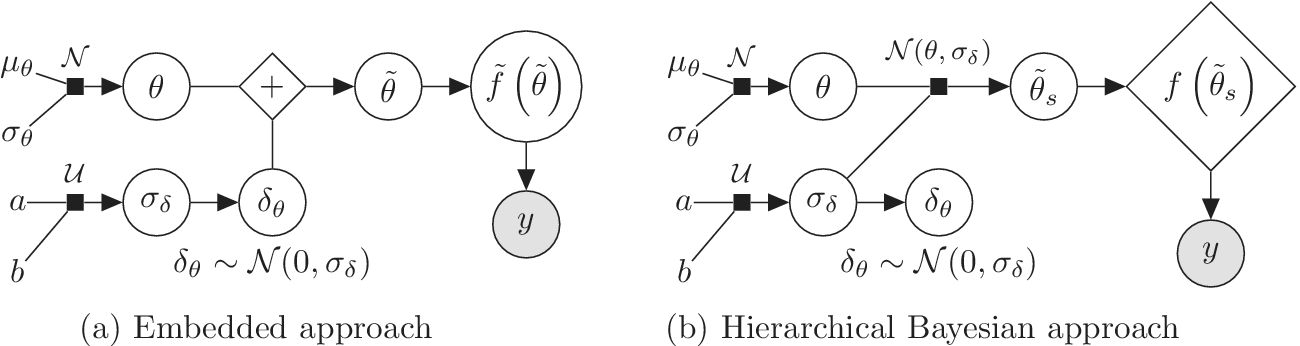

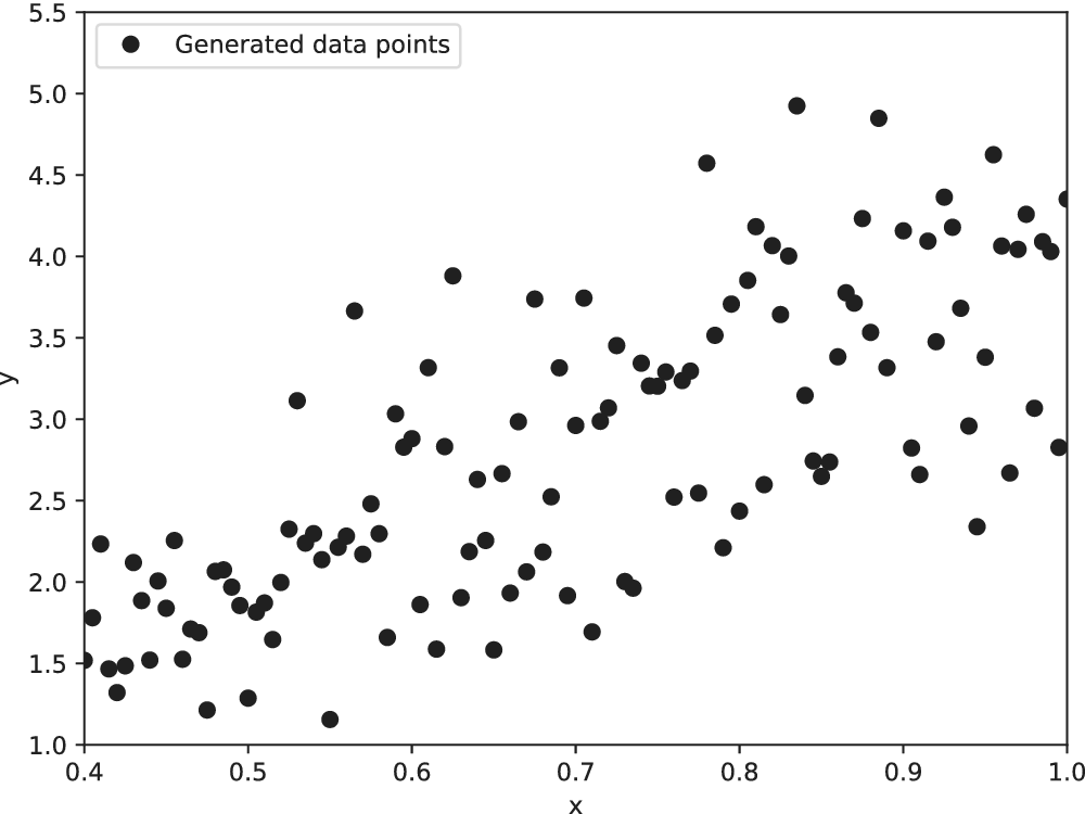


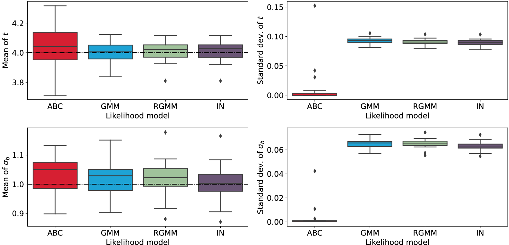


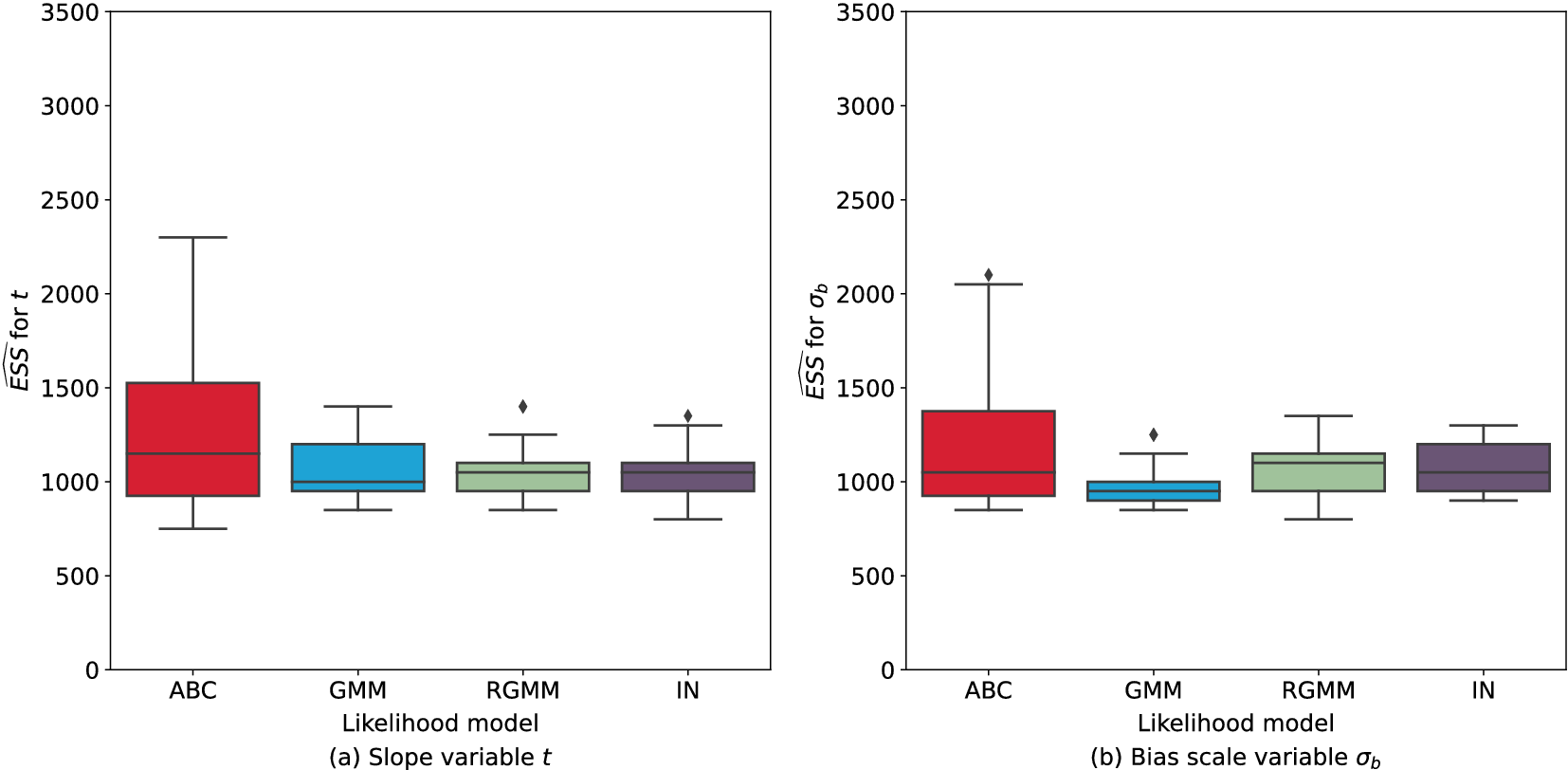


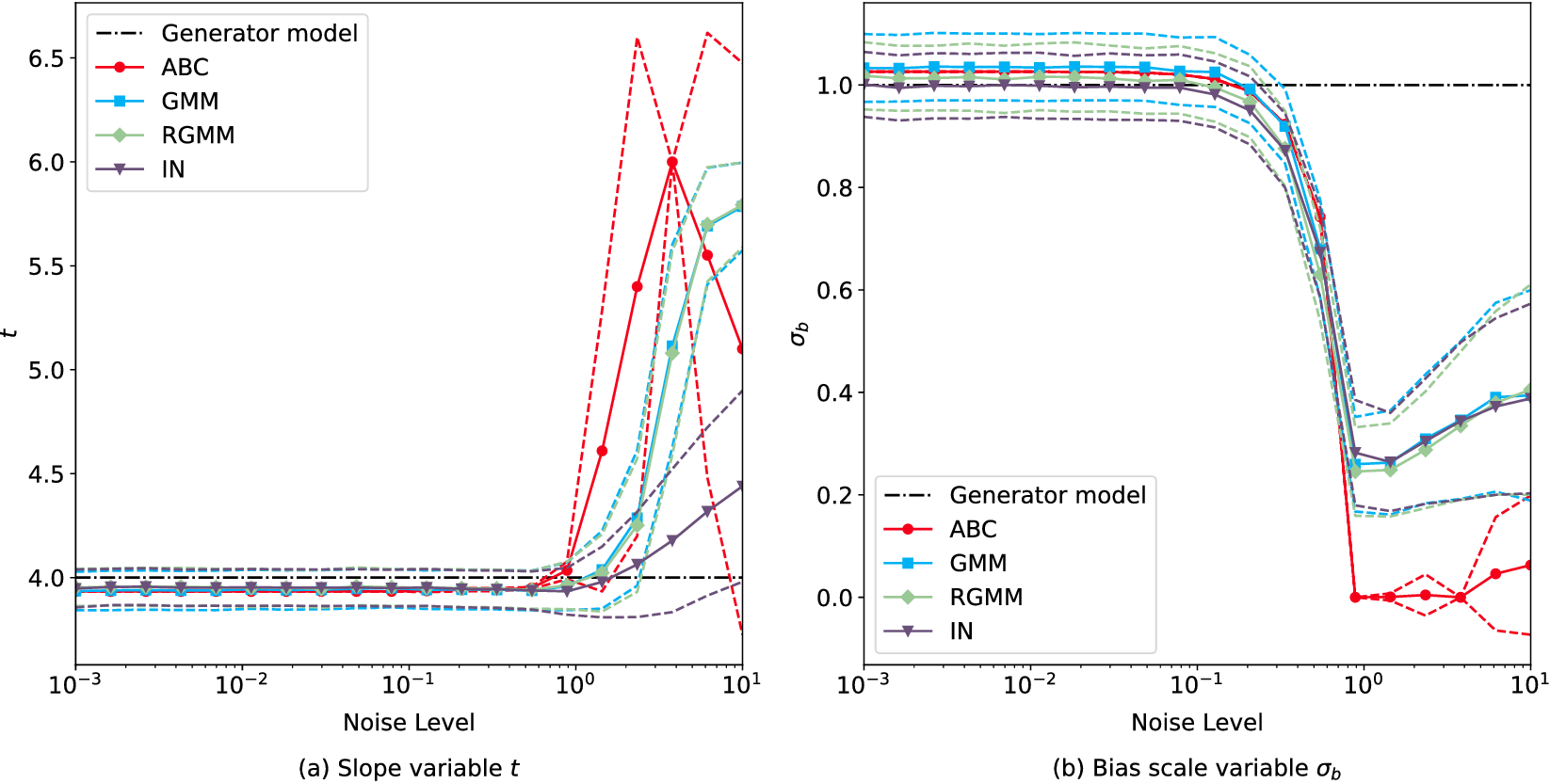


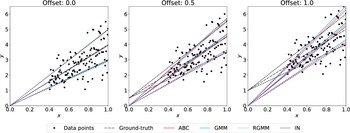
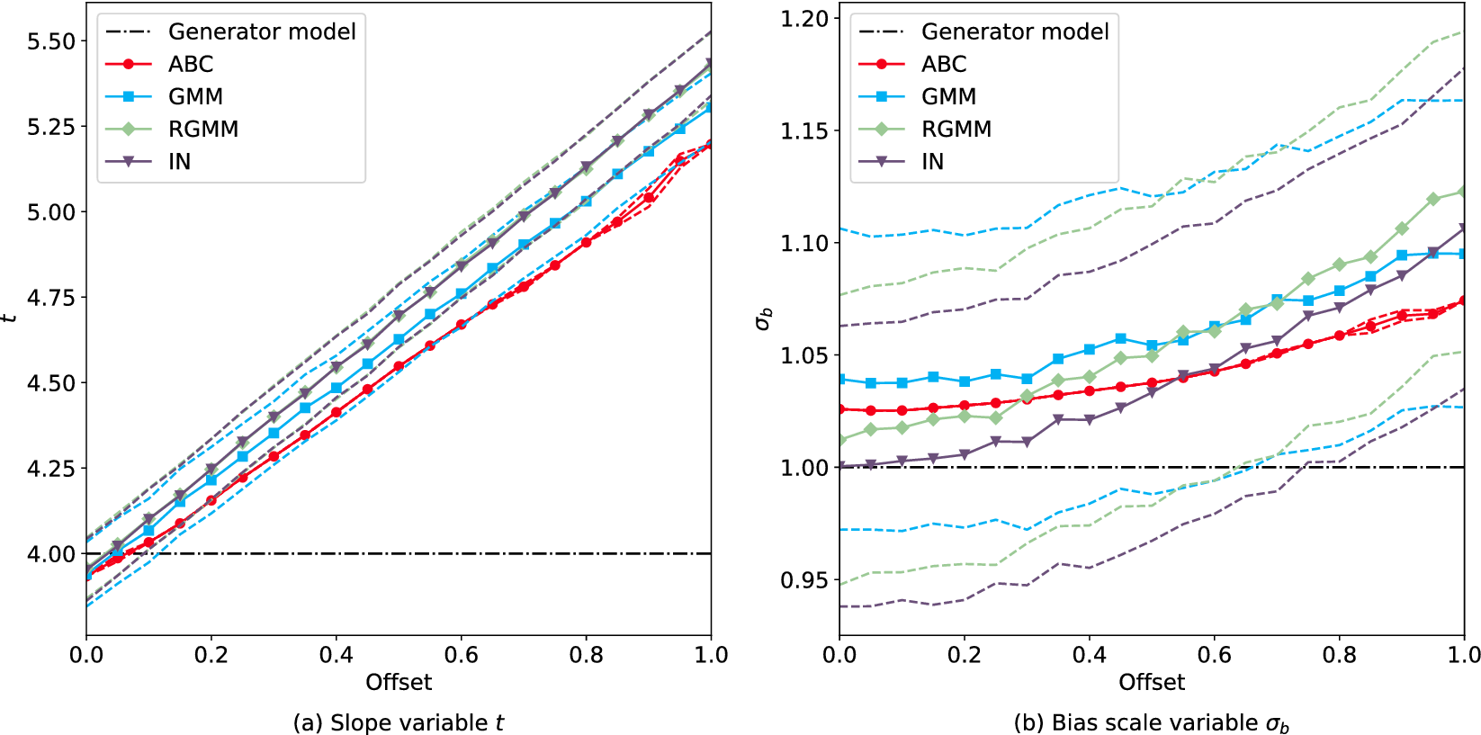


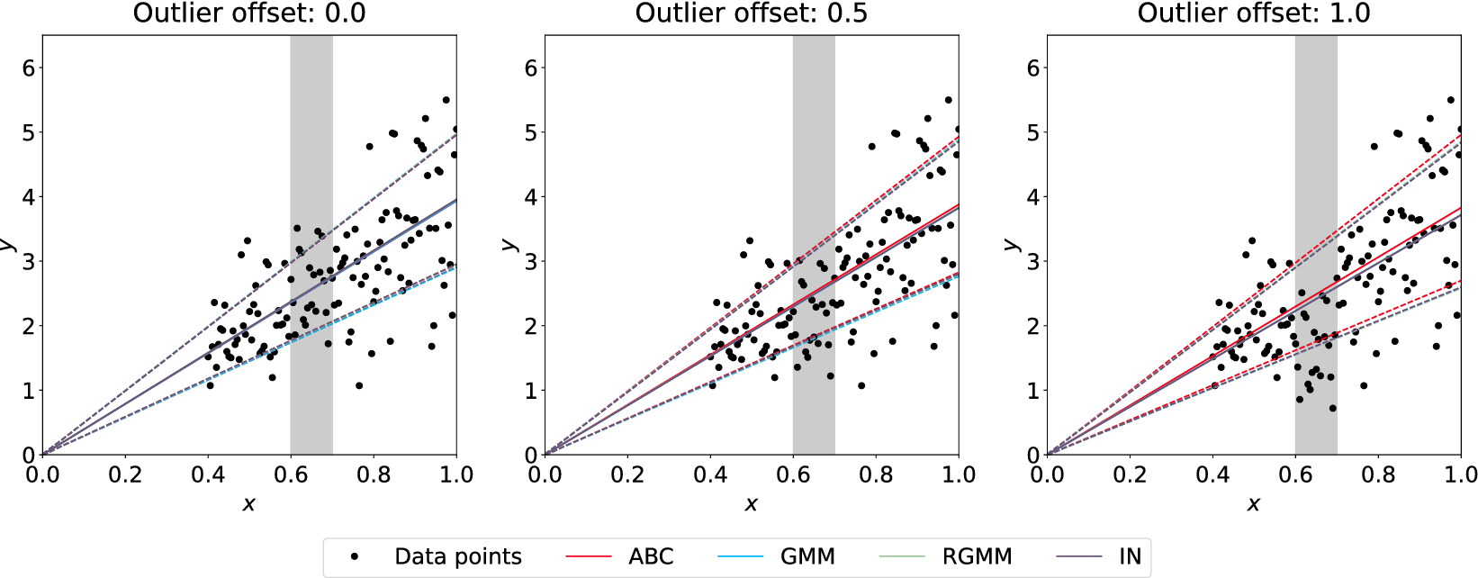


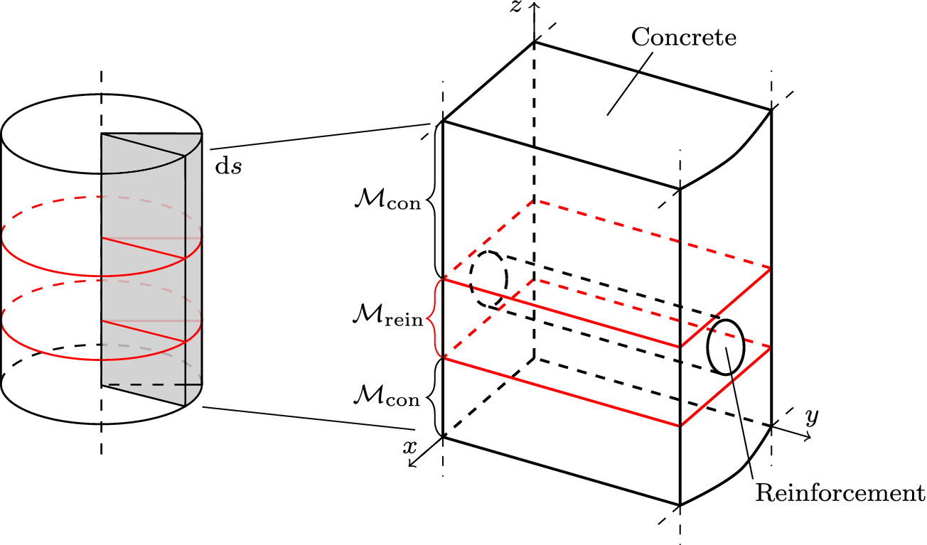

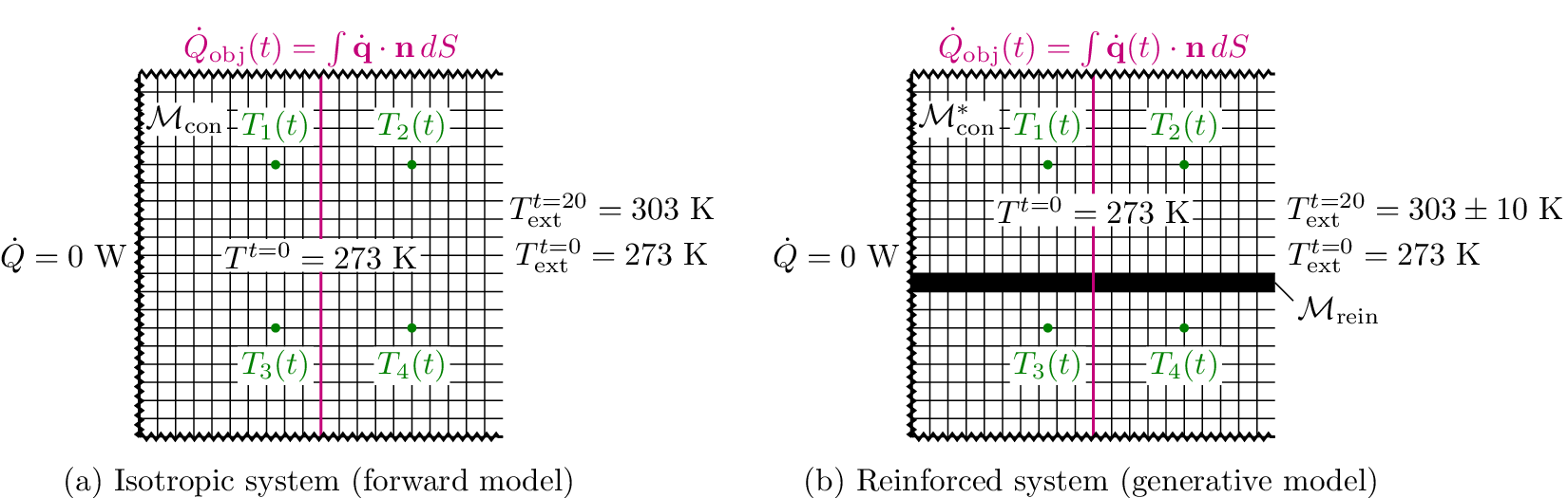


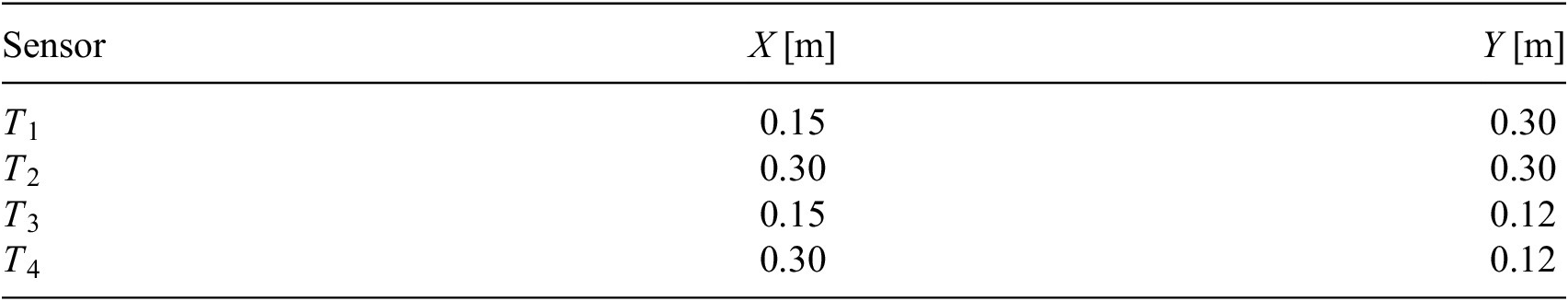
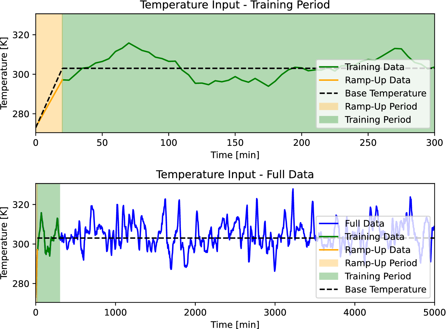


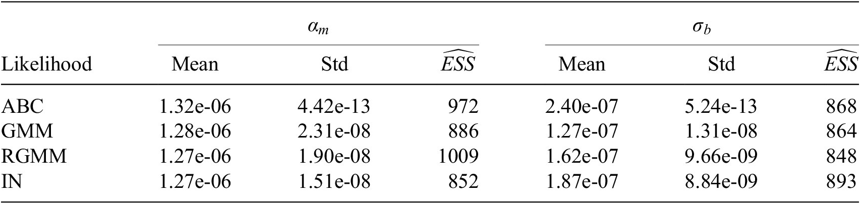
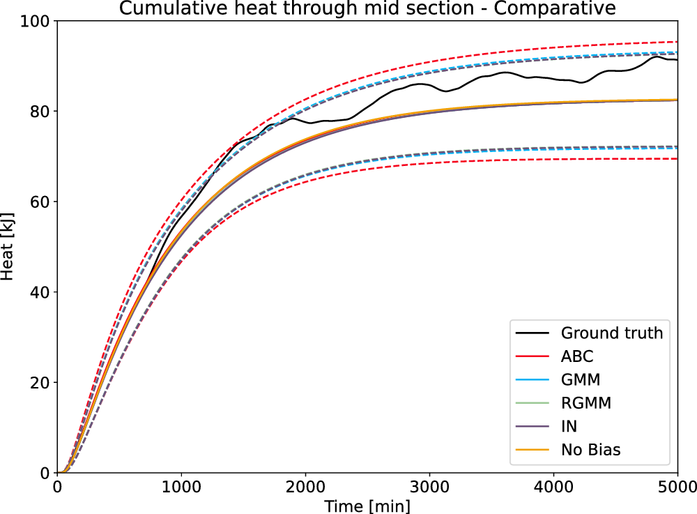


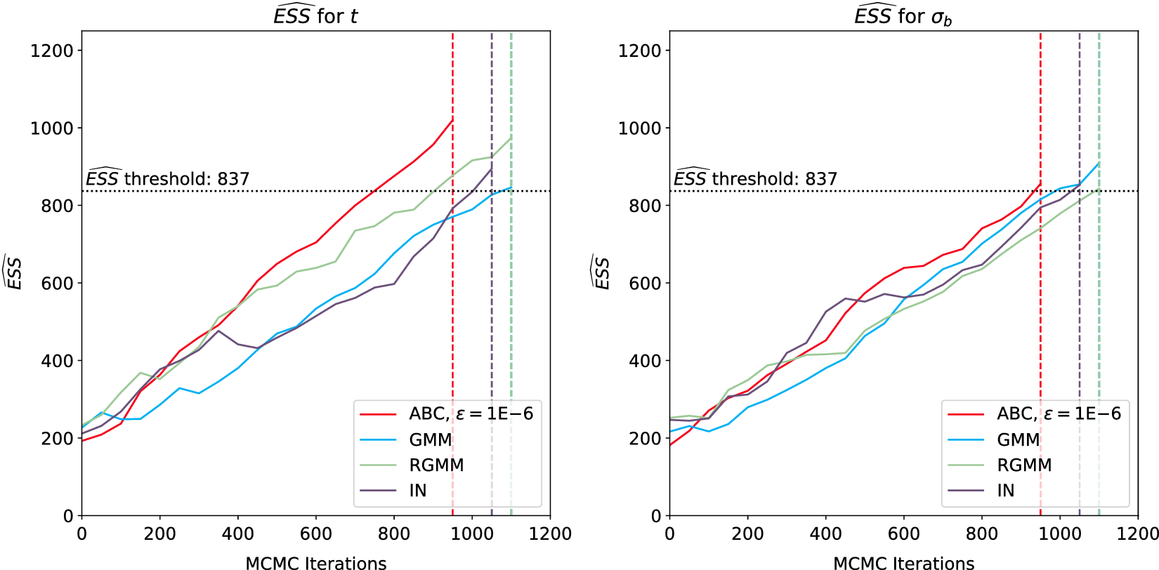


 Open access
Comments
No Comments have been published for this article.