


Impact Statement
Mathematical modeling describing underlying dynamical behaviors plays essential roles in performing engineering studies such as optimization and control. In Complex processes where constructing models from first principles is more challenging, data-driven dynamical models become a valuable tool. The success of data-driven approaches highly relies on the quality of the data. Unlike typical machine learning applications, for example, image classification, data in engineering applications are somewhat limited. Hence, a design of experiments to collect data should be done with care. This paper presents a scheme to collect data with the aim of (heuristically) maximizing the extraction of information with limited measurements. The scheme can be wrapped on top of any existing data-driven modeling methods in a setting.
1. Introduction
In this paper, our focus is on inferring linear time-invariant systems with $ m $
inputs and
$ m $
inputs and $ p $
outputs of the form:
$ p $
outputs of the form:
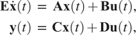 $$ {\displaystyle \begin{array}{c}\mathbf{E}\dot{\mathbf{x}}(t)\hskip0.35em =\hskip0.70em \mathbf{Ax}(t)+\mathbf{Bu}(t),\\ {}\mathbf{y}(t)\hskip0.35em =\hskip0.6em \mathbf{Cx}(t)+\mathbf{Du}(t),\end{array}} $$
from data where $ \mathbf{E},\mathbf{A}\in {\mathrm{\mathbb{R}}}^{n\times n} $
,
$ \mathbf{E},\mathbf{A}\in {\mathrm{\mathbb{R}}}^{n\times n} $
, $ \mathbf{B}\in {\mathrm{\mathbb{R}}}^{n\times m} $
,
$ \mathbf{B}\in {\mathrm{\mathbb{R}}}^{n\times m} $
, $ \mathbf{C}\in {\mathrm{\mathbb{R}}}^{p\times n} $
, and
$ \mathbf{C}\in {\mathrm{\mathbb{R}}}^{p\times n} $
, and $ \mathbf{D}\in {\mathrm{\mathbb{R}}}^{p\times m} $
. Using the Laplace transform, the transfer function
$ \mathbf{D}\in {\mathrm{\mathbb{R}}}^{p\times m} $
. Using the Laplace transform, the transfer function $ \mathbf{H}(s) $
of the system (1) can be obtained and is given as
$ \mathbf{H}(s) $
of the system (1) can be obtained and is given as
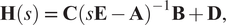 $$ \mathbf{H}(s)\hskip0.35em =\hskip0.35em \mathbf{C}{\left(s\mathbf{E}-\mathbf{A}\right)}^{-1}\mathbf{B}+\mathbf{D}, $$
where $ s $
represents the Laplace domain variable. Although the results presented in this paper can be applied to multi-input multi-output (MIMO) systems, for simplicity, we will focus only on single-input single-output (SISO) systems. The problem of learning dynamical systems of the form (1) is widely studied and well understood (see, e.g., Mayo and Antoulas, Reference Mayo and Antoulas2007; Drmač et al., Reference Drmač, Gugercin and Beattie2015a, Reference Drmač, Gugercin and Beattie2015b; Peherstorfer and Willcox, Reference Peherstorfer and Willcox2016; Antoulas et al., Reference Antoulas, Lefteriu, Ionita, Benner, Cohen, Ohlberger and Willcox2017; Nakatsukasa et al., Reference Nakatsukasa, Sète and Trefethen2018; Brunton and Kutz, Reference Brunton and Kutz2019; Yu et al., Reference Yu, Yan and Guo2019). A key ingredient to data-driven methodologies is data. It is necessary to provide a good data quality, ensuring high fidelity of the inferred model. Typically, there are two possible ways to collect data, namely in frequency domain and time domain. In the frequency domain, transfer function samples are given, whereas, in the time domain, the output
$ s $
represents the Laplace domain variable. Although the results presented in this paper can be applied to multi-input multi-output (MIMO) systems, for simplicity, we will focus only on single-input single-output (SISO) systems. The problem of learning dynamical systems of the form (1) is widely studied and well understood (see, e.g., Mayo and Antoulas, Reference Mayo and Antoulas2007; Drmač et al., Reference Drmač, Gugercin and Beattie2015a, Reference Drmač, Gugercin and Beattie2015b; Peherstorfer and Willcox, Reference Peherstorfer and Willcox2016; Antoulas et al., Reference Antoulas, Lefteriu, Ionita, Benner, Cohen, Ohlberger and Willcox2017; Nakatsukasa et al., Reference Nakatsukasa, Sète and Trefethen2018; Brunton and Kutz, Reference Brunton and Kutz2019; Yu et al., Reference Yu, Yan and Guo2019). A key ingredient to data-driven methodologies is data. It is necessary to provide a good data quality, ensuring high fidelity of the inferred model. Typically, there are two possible ways to collect data, namely in frequency domain and time domain. In the frequency domain, transfer function samples are given, whereas, in the time domain, the output $ \mathbf{y} $
is measured for a given input
$ \mathbf{y} $
is measured for a given input $ \mathbf{u} $
. Moreover, these data may be subject to noise. Depending on an experimental setup, we may collect data in either of these domains.
$ \mathbf{u} $
. Moreover, these data may be subject to noise. Depending on an experimental setup, we may collect data in either of these domains.
Among several widely used approaches, Loewner-based approaches (Mayo and Antoulas, Reference Mayo and Antoulas2007; Antoulas et al., Reference Antoulas, Lefteriu, Ionita, Benner, Cohen, Ohlberger and Willcox2017) to learn dynamical systems have gained increasing popularity. The fundamental idea of the Loewner-based approach is to construct a model that interpolates the given data points in the frequency domain. It has also been extended to time-domain data (Peherstorfer et al., Reference Peherstorfer, Gugercin and Willcox2017). Furthermore, Antoulas et al. (Reference Antoulas, Lefteriu, Ionita, Benner, Cohen, Ohlberger and Willcox2017) have shown that if the minimum order of a system that realizes the system is $ n $
, then using
$ n $
, then using $ 2n $
data points, one can construct the realization using the Loewner approach. However, if only data are given, we cannot know a priori the minimal order of a state-space realization that captures the dynamics of the process. Therefore, typically, one aims at collecting
$ 2n $
data points, one can construct the realization using the Loewner approach. However, if only data are given, we cannot know a priori the minimal order of a state-space realization that captures the dynamics of the process. Therefore, typically, one aims at collecting $ N\gg 2n $
data points, which is then followed by a compression step to determine the minimal order of the state-space model that captures the dynamics of the process. We refer the reader to Mayo and Antoulas (Reference Mayo and Antoulas2007) for more details. However, this approach can impose practical constraints if collecting data are expensive. In this case, we aim to gather data points carefully and focus on collecting the data points to obtain as much information (gathered on the imaginary axis) as possible about the underlying dynamics up to tolerance. In a step toward collecting good data, Beattie and Gugercin (Reference Beattie and Gugercin2012) presented an approach inspired by iterative rational Krylov algorithm (IRKA) (Gugercin et al., Reference Gugercin, Antoulas and Beattie2008) that focused on using interpolation points that facilitate obtaining a model, minimizing the
$ N\gg 2n $
data points, which is then followed by a compression step to determine the minimal order of the state-space model that captures the dynamics of the process. We refer the reader to Mayo and Antoulas (Reference Mayo and Antoulas2007) for more details. However, this approach can impose practical constraints if collecting data are expensive. In this case, we aim to gather data points carefully and focus on collecting the data points to obtain as much information (gathered on the imaginary axis) as possible about the underlying dynamics up to tolerance. In a step toward collecting good data, Beattie and Gugercin (Reference Beattie and Gugercin2012) presented an approach inspired by iterative rational Krylov algorithm (IRKA) (Gugercin et al., Reference Gugercin, Antoulas and Beattie2008) that focused on using interpolation points that facilitate obtaining a model, minimizing the $ {\mathcal{H}}_2 $
error between the learned model and the unknown ground-truth model. However, again, the approach needs the order of the state-space realization as input, which may not be known in advance. In addition, it is an iterative scheme; thus, the number of transfer function evaluations still becomes significantly large. Furthermore, we mention that there also exist other approaches that aim at determining or collecting measurements greedily but require a ground-truth high-fidelity model (see, e.g., Paul-Dubois-Taine and Amsallem, Reference Paul-Dubois-Taine and Amsallem2015; Chellappa et al., Reference Chellappa, Feng and Benner2020; Chellappa et al., Reference Chellappa, Feng, de la Rubia, Benner, Benner, Breiten, Faßbender, Hinze, Stykel and Zimmermann2021; Beddig et al., Reference Beddig, Benner, Dorschky, Reis, Schwerdtner, Voigt and Werner2022).
$ {\mathcal{H}}_2 $
error between the learned model and the unknown ground-truth model. However, again, the approach needs the order of the state-space realization as input, which may not be known in advance. In addition, it is an iterative scheme; thus, the number of transfer function evaluations still becomes significantly large. Furthermore, we mention that there also exist other approaches that aim at determining or collecting measurements greedily but require a ground-truth high-fidelity model (see, e.g., Paul-Dubois-Taine and Amsallem, Reference Paul-Dubois-Taine and Amsallem2015; Chellappa et al., Reference Chellappa, Feng and Benner2020; Chellappa et al., Reference Chellappa, Feng, de la Rubia, Benner, Benner, Breiten, Faßbender, Hinze, Stykel and Zimmermann2021; Beddig et al., Reference Beddig, Benner, Dorschky, Reis, Schwerdtner, Voigt and Werner2022).
On the other hand, our goal is to construct a minimal realization of a process using as few measurement data points as possible up to a tolerance, where we neither know the order of a minimal realization in advance nor have access to any high-fidelity model. Furthermore, one can theoretically consider taking the transfer function measurements on the complex domain, and often, it is known that good, in fact optimal, measurement points are complex as shown in Gugercin et al. (Reference Gugercin, Antoulas and Beattie2008) and Beattie and Gugercin (Reference Beattie and Gugercin2012). However, from an experimental viewpoint and physical interpretation of a transfer function, we assume that transfer function measurements are taken anywhere on the imaginary $ j\omega $
-axis. The motivation of considering measurements on the
$ j\omega $
-axis. The motivation of considering measurements on the $ j\omega $
-axis are:
$ j\omega $
-axis are:
-
(a) A transfer function at $ j\omega $
can be estimated by exciting the system using an input containing sine and cosine functions of the frequency
$ \omega $
. It can be extended to multiple frequencies as well.
$ j\omega $
can be estimated by exciting the system using an input containing sine and cosine functions of the frequency
$ \omega $
. It can be extended to multiple frequencies as well. -
(b) From the control theory perspective, a transfer function can be better interpreted on the
$ j\omega $
-axis, for example, using the Bode plot. More details can be found in, for example, Ogata (Reference Ogata2010).


In this paper, we focus on inferring minimal linear dynamical systems using minimum possible measurement data taken on the imaginary axis up to tolerance, but without knowing the minimal order of the realization a priori and its realization in any form. For this, we discuss a heuristic approach, allowing us to select adaptively frequency points positioned where the transfer function changes the most. We also discuss the extension of the approach to time-domain data.
The paper is structured as follows. In Section 2, the Loewner framework to learn linear dynamical systems is briefly presented. In Section 3, we present the heuristic approach to select frequency points from the imaginary axis (and transfer function measurements) that contributes the most in reducing the error of the obtained realization. Then, in Section 4, we discuss an extension of the approach when input–output data are collected in the time domain. In Section 5, we illustrate the efficiency of the proposed greedy methodology, and compare it with models that are obtained from IRKA and by taking measurements on a uniform grid. Finally, we conclude the paper with a summary and future research in Section 6.
2. Data-Driven Modeling Based on the Loewner Framework
In this section, we briefly recap the Loewner approach (Mayo and Antoulas, Reference Mayo and Antoulas2007) to construct a realization from given transfer function measurements. To that end, for simplicity, we first write down the underlying realization problem for SISO systems—that is as follows.
Problem 2.1.
Given a set of interpolation points $ Z:= \left\{{\sigma}_1,\dots, {\sigma}_{2N}\right\} $
and corresponding transfer function measurements
$ Z:= \left\{{\sigma}_1,\dots, {\sigma}_{2N}\right\} $
and corresponding transfer function measurements $ \mathbf{H}\left({\sigma}_i\right) $
, the goal is to identify a minimal realization whose rational transfer function is denoted by
$ \mathbf{H}\left({\sigma}_i\right) $
, the goal is to identify a minimal realization whose rational transfer function is denoted by $ \hat{\mathbf{H}}(s) $
, satisfying the following interpolation conditions:
$ \hat{\mathbf{H}}(s) $
, satisfying the following interpolation conditions:
 $$ \mathbf{H}\left({\sigma}_i\right)\hskip0.35em =\hskip0.35em \hat{\mathbf{H}}\left({\sigma}_i\right),\hskip1em i\in \left\{1,\dots, 2N\right\}, $$
and the transfer function is given as
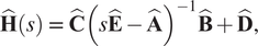 $$ \hat{\mathbf{H}}(s)\hskip0.35em =\hskip0.35em \hat{\mathbf{C}}{\left(s\hat{\mathbf{E}}-\hat{\mathbf{A}}\right)}^{-1}\hat{\mathbf{B}}+\hat{\mathbf{D}}, $$
where $ \hat{\mathbf{E}},\hat{\mathbf{A}}\in {\mathrm{\mathbb{R}}}^{r\times r} $
,
$ \hat{\mathbf{E}},\hat{\mathbf{A}}\in {\mathrm{\mathbb{R}}}^{r\times r} $
, $ \hat{\mathbf{B}}\in {\mathrm{\mathbb{R}}}^r $
,
$ \hat{\mathbf{B}}\in {\mathrm{\mathbb{R}}}^r $
, $ \hat{\mathbf{C}}\in {\mathrm{\mathbb{R}}}^r $
, and
$ \hat{\mathbf{C}}\in {\mathrm{\mathbb{R}}}^r $
, and $ \hat{\mathbf{D}}\in \mathrm{\mathbb{R}} $
with
$ \hat{\mathbf{D}}\in \mathrm{\mathbb{R}} $
with $ r $
being the order of a minimal realization.
$ r $
being the order of a minimal realization.
This realization problem can be solved using the Loewner approach for given $ \hat{\mathbf{D}} $
. For this, we need to split the measurement data into left and right measurements. Let us define the left and right interpolation points as
$ \hat{\mathbf{D}} $
. For this, we need to split the measurement data into left and right measurements. Let us define the left and right interpolation points as $ {\lambda}_j $
and
$ {\lambda}_j $
and $ {\mu}_j $
, where
$ {\mu}_j $
, where $ j\in \left\{1,\dots, N\right\} $
, corresponding transfer function measurements are denoted by
$ j\in \left\{1,\dots, N\right\} $
, corresponding transfer function measurements are denoted by $ \mathbf{H}\left({\lambda}_j\right) $
and
$ \mathbf{H}\left({\lambda}_j\right) $
and $ \mathbf{H}\left({\mu}_j\right) $
, and
$ \mathbf{H}\left({\mu}_j\right) $
, and $ Z\hskip0.35em =\hskip0.35em \left\{{\lambda}_1,\dots, {\lambda}_N\right\}\cup \left\{{\mu}_1,\dots, {\mu}_N\right\} $
. Having these data, in the following, we define the Loewner and shifted Loewner matrices.
$ Z\hskip0.35em =\hskip0.35em \left\{{\lambda}_1,\dots, {\lambda}_N\right\}\cup \left\{{\mu}_1,\dots, {\mu}_N\right\} $
. Having these data, in the following, we define the Loewner and shifted Loewner matrices.
Definition 2.1 (Mayo and Antoulas, Reference Mayo and Antoulas
2007
). Given left data $ \left({\lambda}_j,\mathbf{H}\left({\lambda}_j\right)\right) $
and right data
$ \left({\lambda}_j,\mathbf{H}\left({\lambda}_j\right)\right) $
and right data $ \left({\mu}_j,\mathbf{H}\left({\mu}_j\right)\right) $
, the Loewner
$ \left({\mu}_j,\mathbf{H}\left({\mu}_j\right)\right) $
, the Loewner $ \unicode{x1D543} $
and shifted Loewner
$ \unicode{x1D543} $
and shifted Loewner $ {\unicode{x1D543}}_{\mathrm{s}} $
matrices are defined as
$ {\unicode{x1D543}}_{\mathrm{s}} $
matrices are defined as
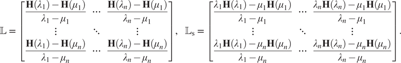 $$ \unicode{x1D543}\hskip0.35em =\hskip0.35em \left[\begin{array}{ccc}\frac{\mathbf{H}\left({\lambda}_1\right)-\mathbf{H}\left({\mu}_1\right)}{\lambda_1-{\mu}_1}& \cdots & \frac{\mathbf{H}\left({\lambda}_n\right)-\mathbf{H}\left({\mu}_1\right)}{\lambda_n-{\mu}_1}\\ {}\vdots & \ddots & \vdots \\ {}\frac{\mathbf{H}\left({\lambda}_1\right)-\mathbf{H}\left({\mu}_n\right)}{\lambda_1-{\mu}_n}& \cdots & \frac{\mathbf{H}\left({\lambda}_n\right)-\mathbf{H}\left({\mu}_n\right)}{\lambda_n-{\mu}_n}\end{array}\right],\hskip1em {\unicode{x1D543}}_{\mathrm{s}}\hskip0.35em =\hskip0.35em \left[\begin{array}{ccc}\frac{\lambda_1\mathbf{H}\left({\lambda}_1\right)-{\mu}_1\mathbf{H}\left({\mu}_1\right)}{\lambda_1-{\mu}_1}& \cdots & \frac{\lambda_n\mathbf{H}\left({\lambda}_n\right)-{\mu}_1\mathbf{H}\left({\mu}_1\right)}{\lambda_n-{\mu}_1}\\ {}\vdots & \ddots & \vdots \\ {}\frac{\lambda_1\mathbf{H}\left({\lambda}_1\right)-{\mu}_n\mathbf{H}\left({\mu}_n\right)}{\lambda_1-{\mu}_n}& \cdots & \frac{\lambda_n\mathbf{H}\left({\lambda}_n\right)-{\mu}_n\mathbf{H}\left({\mu}_n\right)}{\lambda_n-{\mu}_n}\end{array}\right]. $$
It is proved in Mayo and Antoulas (Reference Mayo and Antoulas2007) that based on the Loewner and shifted Loewner matrices, a realization can be constructed that solves Problem 2.1. This result is presented in the following theorem.
Theorem 1 (Mayo and Antoulas, Reference Mayo and Antoulas
2007). Given left data $ \left({\lambda}_j,\mathbf{H}\left({\lambda}_j\right)\right) $
and right data
$ \left({\lambda}_j,\mathbf{H}\left({\lambda}_j\right)\right) $
and right data $ \left({\mu}_j,\mathbf{H}\left({\mu}_j\right)\right) $
, consider the Loewner and shifted Loewner matrices as defined in Definition 2.1. Moreover, assume that the feed-through term
$ \left({\mu}_j,\mathbf{H}\left({\mu}_j\right)\right) $
, consider the Loewner and shifted Loewner matrices as defined in Definition 2.1. Moreover, assume that the feed-through term $ \mathbf{D} $
is known. Then, an interpolating realization can be constructed as below:
$ \mathbf{D} $
is known. Then, an interpolating realization can be constructed as below:
 $$ \hat{\mathbf{E}}\hskip0.35em =\hskip0.35em \unicode{x1D543},\hskip1em \hat{\mathbf{A}}\hskip0.35em =\hskip0.35em {\unicode{x1D543}}_s-\unicode{x1D7D9}\mathbf{D}{\unicode{x1D7D9}}^T,\hskip1em \hat{\mathbf{B}}\hskip0.35em =\hskip0.35em \mathbf{V}-\unicode{x1D7D9}\mathbf{D},\hskip1em \hat{\mathbf{C}}\hskip0.35em =\hskip0.35em \mathbf{W}-\mathbf{D}{\unicode{x1D7D9}}^T,\hskip1em \hat{\mathbf{D}}\hskip0.35em =\hskip0.35em \mathbf{D}, $$
where $ \unicode{x1D7D9}\in {\mathrm{\mathbb{R}}}^N $
is the vector of ones,
$ \unicode{x1D7D9}\in {\mathrm{\mathbb{R}}}^N $
is the vector of ones, $ \hat{\mathbf{E}},\hat{\mathbf{A}}\in {\mathrm{\mathbb{R}}}^{n\times n} $
,
$ \hat{\mathbf{E}},\hat{\mathbf{A}}\in {\mathrm{\mathbb{R}}}^{n\times n} $
, $ \hat{\mathbf{B}}\in {\mathrm{\mathbb{R}}}^n $
,
$ \hat{\mathbf{B}}\in {\mathrm{\mathbb{R}}}^n $
, $ \hat{\mathbf{C}}\in {\mathrm{\mathbb{R}}}^n $
,
$ \hat{\mathbf{C}}\in {\mathrm{\mathbb{R}}}^n $
, $ \hat{\mathbf{D}}\in \mathrm{\mathbb{R}} $
,
$ \hat{\mathbf{D}}\in \mathrm{\mathbb{R}} $
, $ \mathbf{V}\hskip0.35em =\hskip0.35em {\left[\mathbf{H}\left({\lambda}_1\right),\hskip0.5em \dots, \hskip0.5em \mathbf{H}\left({\lambda}_n\right)\right]}^T $
, and
$ \mathbf{V}\hskip0.35em =\hskip0.35em {\left[\mathbf{H}\left({\lambda}_1\right),\hskip0.5em \dots, \hskip0.5em \mathbf{H}\left({\lambda}_n\right)\right]}^T $
, and $ \mathbf{W}\hskip0.35em =\hskip0.35em \left[\begin{array}{ccc}\mathbf{H}\left({\mu}_1\right),& \dots, & \mathbf{H}\left({\mu}_n\right)\end{array}\right] $
. Furthermore, the realization (5) is minimal, assuming
$ \mathbf{W}\hskip0.35em =\hskip0.35em \left[\begin{array}{ccc}\mathbf{H}\left({\mu}_1\right),& \dots, & \mathbf{H}\left({\mu}_n\right)\end{array}\right] $
. Furthermore, the realization (5) is minimal, assuming $ \unicode{x1D543} $
is of full-rank.
$ \unicode{x1D543} $
is of full-rank.
Furthermore, in case the Loewner matrix $ \unicode{x1D543} $
is singular, there exists a lower-order realization of order
$ \unicode{x1D543} $
is singular, there exists a lower-order realization of order $ \hat{n}<n $
, where
$ \hat{n}<n $
, where $ \hat{n}\hskip0.35em =\hskip0.35em \operatorname{rank}\left(\unicode{x1D543}\right) $
, satisfying the interpolation conditions. To remove the redundant information and obtain the minimal realization, a compression step based on the singular-value decomposition (SVD) of
$ \hat{n}\hskip0.35em =\hskip0.35em \operatorname{rank}\left(\unicode{x1D543}\right) $
, satisfying the interpolation conditions. To remove the redundant information and obtain the minimal realization, a compression step based on the singular-value decomposition (SVD) of $ \left[\unicode{x1D543},{\unicode{x1D543}}_{\mathrm{s}}\right] $
can be employed (see, e.g., Mayo and Antoulas, Reference Mayo and Antoulas2007; Antoulas et al., Reference Antoulas, Lefteriu, Ionita, Benner, Cohen, Ohlberger and Willcox2017). We consider here only the minimal realization for systems with an underlying ODE. For high index descriptor systems, one has to be more careful with the definition of minimality (see, e.g., Sokolov, Reference Sokolov2006), which might be interesting to investigate as well in the future in detail. For simplicity, we have presented the realization theory using the Loewner approach for SISO systems; however, it can be extended to MIMO systems using the idea of tangential interpolation. We refer to Mayo and Antoulas (Reference Mayo and Antoulas2007) and Antoulas et al. (Reference Antoulas, Lefteriu, Ionita, Benner, Cohen, Ohlberger and Willcox2017) for more details. We also remark that the realization (5) can be complex if data are complex, but if the data are closed under conjugation, then there exists an orthogonal transformation that allows determining the real realization using that orthogonal transformation.
$ \left[\unicode{x1D543},{\unicode{x1D543}}_{\mathrm{s}}\right] $
can be employed (see, e.g., Mayo and Antoulas, Reference Mayo and Antoulas2007; Antoulas et al., Reference Antoulas, Lefteriu, Ionita, Benner, Cohen, Ohlberger and Willcox2017). We consider here only the minimal realization for systems with an underlying ODE. For high index descriptor systems, one has to be more careful with the definition of minimality (see, e.g., Sokolov, Reference Sokolov2006), which might be interesting to investigate as well in the future in detail. For simplicity, we have presented the realization theory using the Loewner approach for SISO systems; however, it can be extended to MIMO systems using the idea of tangential interpolation. We refer to Mayo and Antoulas (Reference Mayo and Antoulas2007) and Antoulas et al. (Reference Antoulas, Lefteriu, Ionita, Benner, Cohen, Ohlberger and Willcox2017) for more details. We also remark that the realization (5) can be complex if data are complex, but if the data are closed under conjugation, then there exists an orthogonal transformation that allows determining the real realization using that orthogonal transformation.
The success of the Loewner approach has been shown in various applications (see, e.g., Ionita and Antoulas, Reference Ionita, Antoulas, Quarteroni and Rozza2014a, Reference Ionita and Antoulas2014b; Poussot-Vassal et al., Reference Poussot-Vassal, Kergus, Kerhervé, Sipp and Cordier2021). Its success lies in the quality of data and assumes that there are enough data for a wide range of frequencies. However, suppose that the data collection process is expensive. In this case, it is essential to make a smart choice to measurements to maximize information about the system with limited data. With this aim, in the following section, we discuss an adaptive scheme to collect measurements to extract more information about the system, as compared to the standard equidistant measurements on the imaginary axis, with a fixed number of measurements.
3. A Greedy-Based Data Collection Scheme
Naturally, the quality of collected data is a key ingredient to learning a good and reliable model, describing the underlying dynamics of a process. Obviously, one can collect as much data as possible if feasible. It can then be followed by inferring a system realization by using, for example, the Loewner approach (Mayo and Antoulas, Reference Mayo and Antoulas2007) as discussed in the previous section. However, a mass collection could be expensive in many scenarios. Therefore, in this section, we discuss a greedy scheme that can guide us to collect the data, so that we can expect to extract as much new information about the dynamical system from every measurement taken on the imaginary axis as possible. In the following, we first note down a corresponding problem.
Problem 3.1. Identify the underlying state-space dynamical system of a process using a minimal number of transfer function evaluations restricted to the imaginary axis up to a user-defined tolerance.
To that end, we first assume that we have an initial rough construct of a realization that still can be far from satisfactory. An initial rough model can be constructed using only a few measurement points. We denote the transfer function of the initial realization by $ {\mathbf{H}}_{\mathtt{init}}(s) $
. Furthermore, let us denote the transfer function of the unknown ground truth realization by
$ {\mathbf{H}}_{\mathtt{init}}(s) $
. Furthermore, let us denote the transfer function of the unknown ground truth realization by $ {\mathbf{H}}_{\mathtt{true}}(s) $
. In this case, we ideally would like to update the model using the point on the
$ {\mathbf{H}}_{\mathtt{true}}(s) $
. In this case, we ideally would like to update the model using the point on the $ j\omega $
-axis, where the maximum error between the true and initial realized systems occurs; hence, we select the interpolation point that solves the following optimization problem:
$ j\omega $
-axis, where the maximum error between the true and initial realized systems occurs; hence, we select the interpolation point that solves the following optimization problem:
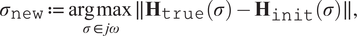 $$ {\sigma}_{\mathtt{new}}:= \underset{\sigma \in j\omega}{\arg \max}\parallel {\mathbf{H}}_{\mathtt{true}}\left(\sigma \right)-{\mathbf{H}}_{\mathtt{init}}\left(\sigma \right)\parallel, $$
where $ \omega \in \mathrm{\mathbb{R}}. $
However, to solve the optimization problem (6), we require the transfer function of the ground-truth realization, which is not available. Therefore, we seek for an alternative approach, allowing us to estimate good interpolation points in an iterative procedure. For this, let us assume that we have
$ \omega \in \mathrm{\mathbb{R}}. $
However, to solve the optimization problem (6), we require the transfer function of the ground-truth realization, which is not available. Therefore, we seek for an alternative approach, allowing us to estimate good interpolation points in an iterative procedure. For this, let us assume that we have $ 2k $
measurement points, to begin with, and denote these measurements by tuples
$ 2k $
measurement points, to begin with, and denote these measurements by tuples $ \left({\sigma}_i,\mathbf{H}\left({\sigma}_i\right)\right) $
,
$ \left({\sigma}_i,\mathbf{H}\left({\sigma}_i\right)\right) $
, $ i\in \left\{1,\dots, 2k\right\} $
, where
$ i\in \left\{1,\dots, 2k\right\} $
, where $ {\sigma}_i $
and
$ {\sigma}_i $
and $ \mathbf{H}\left({\sigma}_i\right) $
are the interpolation points and the transfer function measurements at these points. Before we proceed further, we define the following notation:
$ \mathbf{H}\left({\sigma}_i\right) $
are the interpolation points and the transfer function measurements at these points. Before we proceed further, we define the following notation:
-
•
$ {\Sigma}_i:= \left\{{\sigma}_1,\dots, {\sigma}_{2i}\right\}. $
-
• The transfer function of the realization constructed using interpolation points
$ {\Sigma}_m $
is denoted by
$ {\mathbf{H}}_m(s) $
, and the order of the constructed realization is
$ m $
.


Next, we construct realizations using interpolation points $ {\Sigma}_{k-1}\subset {\Sigma}_k $
and
$ {\Sigma}_{k-1}\subset {\Sigma}_k $
and $ {\Sigma}_k $
, which are, respectively, denoted by
$ {\Sigma}_k $
, which are, respectively, denoted by $ {\mathbf{H}}_{k-1}(s) $
and
$ {\mathbf{H}}_{k-1}(s) $
and $ {\mathbf{H}}_k(s) $
. As discussed earlier, we ideally would add a new measurement for the next
$ {\mathbf{H}}_k(s) $
. As discussed earlier, we ideally would add a new measurement for the next $ {\mathbf{H}}_{k+1}(s) $
realization at the frequency that solves the problem (6). Since we do not know
$ {\mathbf{H}}_{k+1}(s) $
realization at the frequency that solves the problem (6). Since we do not know $ {\mathbf{H}}_{\mathtt{true}} $
, in the following, we discuss a heuristic approach to relax the optimization problem. First note that
$ {\mathbf{H}}_{\mathtt{true}} $
, in the following, we discuss a heuristic approach to relax the optimization problem. First note that
 $$ {\displaystyle \begin{array}{l}\parallel {\mathbf{H}}_{\mathtt{true}}\left(\sigma \right)-{\mathbf{H}}_k\left(\sigma \right)\parallel \hskip0.35em =\hskip0.35em \parallel {\mathbf{H}}_{\mathtt{true}}\left(\sigma \right)-{\mathbf{H}}_{k-1}\left(\sigma \right)-\left({\mathbf{H}}_k\left(\sigma \right)-{\mathbf{H}}_{k-1}\left(\sigma \right)\right)\parallel \\ {}\hskip16.5em \le \parallel {\mathbf{H}}_{\mathtt{true}}\left(\sigma \right)-{\mathbf{H}}_{k-1}\left(\sigma \right)\parallel +\parallel {\mathbf{H}}_k\left(\sigma \right)-{\mathbf{H}}_{k-1}\left(\sigma \right)\parallel .\end{array}} $$
With unknown $ {\mathbf{H}}_{\mathtt{true}}\left(\sigma \right) $
, we rather focus on defining our next measurements data based on the second part of (7) with a constraint; that is, we should exclude the regime of already taken measurements points. Hence, we solve an optimization problem to obtain a frequency point at which transfer function measurement needs to be taken to obtain more information about the underlying dynamics:
$ {\mathbf{H}}_{\mathtt{true}}\left(\sigma \right) $
, we rather focus on defining our next measurements data based on the second part of (7) with a constraint; that is, we should exclude the regime of already taken measurements points. Hence, we solve an optimization problem to obtain a frequency point at which transfer function measurement needs to be taken to obtain more information about the underlying dynamics:
 $$ \underset{\sigma \in j\omega}{\max}\;\mathbf{g}\left(\sigma \right)\parallel {\mathbf{H}}_k\left(\sigma \right)-{\mathbf{H}}_{k-1}\left(\sigma \right)\parallel, $$
where the function $ \mathbf{g}\left(\sigma \right) $
can be thought of as a mask that aims at excluding the regime of points at which measurements have already been collected. If
$ \mathbf{g}\left(\sigma \right) $
can be thought of as a mask that aims at excluding the regime of points at which measurements have already been collected. If $ \mathbf{g}\left(\sigma \right) $
is known, then we can solve (8) to obtain our new measurement points which possibly bring the most information about the system as they would occur at the maximum change in the transfer function from the previous to the next step. It is worth noting that
$ \mathbf{g}\left(\sigma \right) $
is known, then we can solve (8) to obtain our new measurement points which possibly bring the most information about the system as they would occur at the maximum change in the transfer function from the previous to the next step. It is worth noting that $ \parallel {\mathbf{H}}_k\left(\sigma \right)-{\mathbf{H}}_{k-1}\left(\sigma \right)\parallel $
could be replaced by an indicator that is cheaper to evaluate than sampling the system and that would reduce the cost of the optimization process (8).
$ \parallel {\mathbf{H}}_k\left(\sigma \right)-{\mathbf{H}}_{k-1}\left(\sigma \right)\parallel $
could be replaced by an indicator that is cheaper to evaluate than sampling the system and that would reduce the cost of the optimization process (8).
Naturally, the choice of the function $ \mathbf{g}\left(\cdot \right) $
in (8) plays an important role in determining next measurement points. Therefore, in the following, we discuss a choice of the mask function
$ \mathbf{g}\left(\cdot \right) $
in (8) plays an important role in determining next measurement points. Therefore, in the following, we discuss a choice of the mask function $ \mathbf{g}\left(\sigma \right) $
. As discussed, a choice of the mask function should be such that it excludes the regime of already considered data points. Among many possible choices, here, we propose the following choice:
$ \mathbf{g}\left(\sigma \right) $
. As discussed, a choice of the mask function should be such that it excludes the regime of already considered data points. Among many possible choices, here, we propose the following choice:
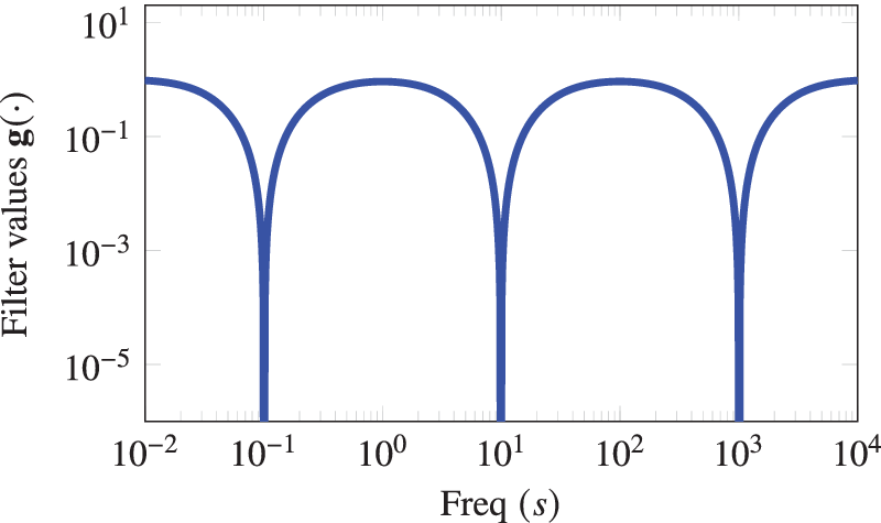
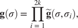 $$ \mathbf{g}\left(\sigma \right)\hskip0.35em =\hskip0.35em \prod \limits_{i\hskip0.35em =\hskip0.35em 1}^{2k}\tilde{\mathbf{g}}\left(\sigma, {\sigma}_i\right), $$
where $ \tilde{\mathbf{g}}\left(\sigma, {\sigma}_i\right) $
is defined as
$ \tilde{\mathbf{g}}\left(\sigma, {\sigma}_i\right) $
is defined as
 $$ \tilde{\mathbf{g}}\left(\sigma, {\sigma}_i\right)\hskip0.35em =\hskip0.35em 1-{\mathrm{e}}^{\left(-\beta {\left(\log \left(|\sigma |+\varepsilon \right)-\log \left(|{\sigma}_i|+\varepsilon \right)\right)}^2\right)}, $$
with $ {\sigma}_i,i\in \left\{1,\dots, 2k\right\} $
, being already considered measurement points, and
$ {\sigma}_i,i\in \left\{1,\dots, 2k\right\} $
, being already considered measurement points, and $ \varepsilon $
and
$ \varepsilon $
and $ \beta $
are positive constants and hyperparameters. It can be noticed that
$ \beta $
are positive constants and hyperparameters. It can be noticed that $ \mathbf{g}\left(\sigma \right) $
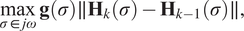
is zero at all the considered points with small values in their neighborhood in order to favor the exploration over the already chosen interpolation points. The mask function can also be seen as a notch filter at multiple frequencies and
$ \mathbf{g}\left(\sigma \right) $
is zero at all the considered points with small values in their neighborhood in order to favor the exploration over the already chosen interpolation points. The mask function can also be seen as a notch filter at multiple frequencies and $ \beta $
can be seen as the bandwidth of the filter. To illustrate the mask function, we plot the function for
$ \beta $
can be seen as the bandwidth of the filter. To illustrate the mask function, we plot the function for $ \beta \hskip0.35em =\hskip0.35em 0.6 $
,
$ \beta \hskip0.35em =\hskip0.35em 0.6 $
, $ \varepsilon \hskip0.35em =\hskip0.35em {10}^{-15} $
, and the notch frequencies
$ \varepsilon \hskip0.35em =\hskip0.35em {10}^{-15} $
, and the notch frequencies $ {\sigma}_i\hskip0.35em =\hskip0.35em \left\{{10}^{-1},{10}^1,{10}^3\right\} $
in Figure 1. It clearly shows that the mask takes smaller values near the considered frequency points.
$ {\sigma}_i\hskip0.35em =\hskip0.35em \left\{{10}^{-1},{10}^1,{10}^3\right\} $
in Figure 1. It clearly shows that the mask takes smaller values near the considered frequency points.
A visual illustration of the filter when the measurements are already taken at the frequencies $ {\sigma}_i=\left\{{10}^{-1},{10}^1,{10}^3\right\} $
.
$ {\sigma}_i=\left\{{10}^{-1},{10}^1,{10}^3\right\} $
.
Next, we discuss how to further simplify the choice of the function $ \mathbf{g}\left(\sigma \right) $
. First, note that
$ \mathbf{g}\left(\sigma \right) $
. First, note that $ {\mathbf{H}}_k\left({\sigma}_i\right)\hskip0.35em =\hskip0.35em {\mathbf{H}}_{k-1}\left({\sigma}_i\right) $
, for
$ {\mathbf{H}}_k\left({\sigma}_i\right)\hskip0.35em =\hskip0.35em {\mathbf{H}}_{k-1}\left({\sigma}_i\right) $
, for $ i\in \left\{1,\dots, 2k-2\right\} $
, assuming that the realization is determined by the Loewner approach, and thus, the interpolation at the given measurement points is exact. As a result, we can also consider the optimization problem to determine our next measurement point as follows:
$ i\in \left\{1,\dots, 2k-2\right\} $
, assuming that the realization is determined by the Loewner approach, and thus, the interpolation at the given measurement points is exact. As a result, we can also consider the optimization problem to determine our next measurement point as follows:
 $$ {\sigma}_{2k+1}:= \arg \hskip0.1em {\max}_{\sigma \in j\omega}\prod \limits_{i\hskip0.35em =\hskip0.35em 2k-1}^{2k}\tilde{\mathbf{g}}\left(\sigma, {\sigma}_i\right)\parallel {\mathbf{H}}_k\left(\sigma \right)-{\mathbf{H}}_{k-1}\left(\sigma \right)\parallel . $$
In this paper, we utilize the Loewner approach to construct the realization. Therefore, it is preferred to have an even number of measurement points to avoid the construction of a rectangular and imaginary realization. Hence, it is desired to include two new additional points at each step. Consequently, in order to choose one additional point, we solve the following optimization problem once $ {\sigma}_{2k+1} $
is obtained:
$ {\sigma}_{2k+1} $
is obtained:
 $$ {\sigma}_{2k+2}:= \underset{\sigma \in j\omega}{\arg \hskip0.1em \max}\prod \limits_{i\hskip0.35em =\hskip0.35em 2k-1}^{2k+1}\tilde{\mathbf{g}}\left(\sigma, {\sigma}_i\right)\parallel {\mathbf{H}}_k\left(\sigma \right)-{\mathbf{H}}_{k-1}\left(\sigma \right)\parallel . $$
As a result, we have two new frequency points $ {\sigma}_{2k+1} $
and
$ {\sigma}_{2k+1} $
and $ {\sigma}_{2k+2} $
at which we take transfer function measurements. Thus, we update our realization
$ {\sigma}_{2k+2} $
at which we take transfer function measurements. Thus, we update our realization $ {\mathbf{H}}_{k+1} $
by using measurements at
$ {\mathbf{H}}_{k+1} $
by using measurements at $ {\sigma}_i $
,
$ {\sigma}_i $
, $ i\in \left\{1,\dots, 2k+2\right\} $
. In the SISO case, the norm between the transfer function measurements just becomes the absolute value. The whole procedure is repeated until the error between two iterations is small enough, that is,
$ i\in \left\{1,\dots, 2k+2\right\} $
. In the SISO case, the norm between the transfer function measurements just becomes the absolute value. The whole procedure is repeated until the error between two iterations is small enough, that is,
 $$ \underset{s\in j\omega}{\max}\parallel {\mathbf{H}}_k(s)-{\mathbf{H}}_{k-1}(s)\parallel \le \mathtt{tol}. $$
We sketch the whole procedure in Algorithm 1. When the condition (12) is met, the algorithm terminates as we have obtained the minimal realization of the system with respect to the given tolerance.
Moreover, we point out that the algorithm is not sensitive to small changes in the input hyperparameters. For example, a small change in $ \beta $
in the mask function will not significantly impact the convergence of the algorithm as long as the mask function keeps the properties described above. This is discussed more in the numerical section. The other hyperparameter
$ \beta $
in the mask function will not significantly impact the convergence of the algorithm as long as the mask function keeps the properties described above. This is discussed more in the numerical section. The other hyperparameter $ \mathtt{tol} $
needs to be set by the user as a trade-off between the accuracy of the resulting model and the number of interpolation points used.
$ \mathtt{tol} $
needs to be set by the user as a trade-off between the accuracy of the resulting model and the number of interpolation points used.
Algorithm 1. A greedy selection of measurement points in the frequency domain.
Input: A parameter $ \beta $
, and initial measurement points
$ \beta $
, and initial measurement points $ {\Sigma}_k:= \left\{{\sigma}_1,\dots, {\sigma}_{2k}\right\} $
.
$ {\Sigma}_k:= \left\{{\sigma}_1,\dots, {\sigma}_{2k}\right\} $
.
-
1 Determine realizations
$ {\mathbf{H}}_{k-1} $
and
$ {\mathbf{H}}_k $
by using measurement points
$ {\Sigma}_{k-1}\subset {\Sigma}_k $
and
$ {\Sigma}_k $
, respectively, and by employing the Loewner approach. -
2 Compute
$ \mathtt{Err}:= \underset{s\in j\omega}{\max}\parallel {\mathbf{H}}_k(s)-{\mathbf{H}}_{k-1}(s)\parallel $
. -
3 while
$ \mathtt{Err}>tol $
do


Output: A learned model, whose transfer function is given by $ {\mathbf{H}}_k $
.
$ {\mathbf{H}}_k $
.
4. Extension to Time-Domain Data
In the previous section, we have discussed a greedy approach for frequency-domain measurements. Here, we suppose that we have access to the time-domain data instead of the frequency-domain data. In this case, we need to design input to collect time-domain data, so that we can maximize information extraction about the process. In this case, we can also employ Algorithm 1 with a slight modification. First, note that Peherstorfer et al. (Reference Peherstorfer, Gugercin and Willcox2017) have proposed a methodology to realize a state-space model using time-domain data, where frequency-domain measurements are estimated using time-domain data. This is followed by obtaining a realization using the Loewner framework described in Section 2. However, the methodology heavily depends on the choice of input, and the choice should be made in such a way that it allows us to describe the dynamics of the system completely. Hence, in this section, we discuss a suitable choice of inputs. Using an extension of Algorithm 1, one can adaptively choose frequency points composing an input. In practice, time-domain measurements are typically collected at a regular interval; hence, the measurements are discrete. Therefore, the proposed greedy procedure needs to be adapted in a discrete setting. In what follows, we discuss the adaptation that needs to be made to allow us to design an input to extract as much information as possible. Note that the interpolation points are no longer on the $ s\hbox{-} $
plane but are rather on the unit circle of the
$ s\hbox{-} $
plane but are rather on the unit circle of the $ z\hbox{-} $
plane. Thus, the frequency range on the
$ z\hbox{-} $
plane. Thus, the frequency range on the $ j\omega $
-axis needs to be mapped on the unit circle using an appropriate discretization method. The Cayley transform could be used to map between the discrete-time and continuous-time systems. To obtain time-domain measurements, the system is excited with an input spanning a set of interpolation points, and the system response is measured. We design an input
$ j\omega $
-axis needs to be mapped on the unit circle using an appropriate discretization method. The Cayley transform could be used to map between the discrete-time and continuous-time systems. To obtain time-domain measurements, the system is excited with an input spanning a set of interpolation points, and the system response is measured. We design an input $ {\mathbf{u}}_p^{(k)} $
using a sum of sine and cosine functions, that is, the input in the
$ {\mathbf{u}}_p^{(k)} $
using a sum of sine and cosine functions, that is, the input in the $ k $
th step of the algorithm at time
$ k $
th step of the algorithm at time $ {\mathbf{T}}_sp $
, where
$ {\mathbf{T}}_sp $
, where $ {\mathbf{T}}_s $
is a sampling time, and
$ {\mathbf{T}}_s $
is a sampling time, and $ p $
is a nonnegative integer, can be given in the form:
$ p $
is a nonnegative integer, can be given in the form:
 $$ {\mathbf{u}}_p^{(k)}\hskip0.35em =\hskip0.35em \frac{1}{K}\sum \limits_{l\hskip0.35em =\hskip0.35em 1}^2\left(1+j\right)\left(\cos \left({\sigma}_{2k+l}\right)+j\sin \left({\sigma}_{2k+l}\right)\right), $$
where $ j:= \sqrt{-1} $
,
$ j:= \sqrt{-1} $
, $ p\in \left\{0,\dots, K-1\right\} $
, and
$ p\in \left\{0,\dots, K-1\right\} $
, and $ K $
is the number of time-domain measurements.
$ K $
is the number of time-domain measurements.
Following the same strategy as in Section 3, the goal is to estimate frequency-domain data, corresponding transfer function estimates, and construct a realization using the interpolation points. However, since only time-domain data are available, one has first to use these data to estimate the frequency measurements.
The complete procedure is as follows. Given an initial realization $ {\mathbf{H}}_{\mathtt{init}}(s) $
, the next two interpolation points
$ {\mathbf{H}}_{\mathtt{init}}(s) $
, the next two interpolation points $ {\sigma}_{2k+1} $
and
$ {\sigma}_{2k+1} $
and $ {\sigma}_{2k+2} $
are computed as in (10) and (11). Then, we construct the input
$ {\sigma}_{2k+2} $
are computed as in (10) and (11). Then, we construct the input $ {\mathbf{u}}_p^{(k)} $
(at step
$ {\mathbf{u}}_p^{(k)} $
(at step $ k $
of the algorithm and time step
$ k $
of the algorithm and time step $ p $
) as in (13) with the two interpolation points
$ p $
) as in (13) with the two interpolation points $ {\sigma}_{2k+1} $
and
$ {\sigma}_{2k+1} $
and $ {\sigma}_{2k+2} $
. We simulate the system to obtain an output having a value of
$ {\sigma}_{2k+2} $
. We simulate the system to obtain an output having a value of $ {\mathbf{y}}_p^{(k)} $
at the step
$ {\mathbf{y}}_p^{(k)} $
at the step $ k $
of the algorithm and at time step
$ k $
of the algorithm and at time step $ p $
. Assembling this time-domain data, one can then compute estimates for the transfer function
$ p $
. Assembling this time-domain data, one can then compute estimates for the transfer function $ {\mathbf{H}}_{\mathtt{true}}\left({\sigma}_{2k+1}\right) $
and
$ {\mathbf{H}}_{\mathtt{true}}\left({\sigma}_{2k+1}\right) $
and $ {\mathbf{H}}_{\mathtt{true}}\left({\sigma}_{2k+2}\right) $
. These values are computed using the following least-squares problem (Peherstorfer et al., Reference Peherstorfer, Gugercin and Willcox2017):
$ {\mathbf{H}}_{\mathtt{true}}\left({\sigma}_{2k+2}\right) $
. These values are computed using the following least-squares problem (Peherstorfer et al., Reference Peherstorfer, Gugercin and Willcox2017):
 $$ \underset{\hat{\mathbf{H}}\in {\mathrm{\mathbb{C}}}^r}{\arg \min}\hskip0.1em {\left\Vert \mathbf{F}\hat{\mathbf{H}}-\overline{\mathbf{y}}\right\Vert}_2^2, $$
where $ \mathbf{F}\in {\mathrm{\mathbb{C}}}^{\left(\mathbf{K}-{k}_{\mathrm{min}}\right)\times 2} $
and
$ \mathbf{F}\in {\mathrm{\mathbb{C}}}^{\left(\mathbf{K}-{k}_{\mathrm{min}}\right)\times 2} $
and $ \hat{\mathbf{H}} $
are described below:
$ \hat{\mathbf{H}} $
are described below:
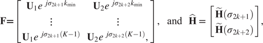
where $ \tilde{\mathbf{H}}\left(\sigma \right) $
is an estimate of
$ \tilde{\mathbf{H}}\left(\sigma \right) $
is an estimate of $ {\mathbf{H}}_{\mathtt{true}}\left(\sigma \right) $
, and the output vector is defined as
$ {\mathbf{H}}_{\mathtt{true}}\left(\sigma \right) $
, and the output vector is defined as $ \overline{\mathbf{y}}:= {\left[{\mathbf{y}}_{k_{\mathrm{min}}}^{(k)},\dots, {\mathbf{y}}_{K-1}^{(k)}\right]}^T $
such that
$ \overline{\mathbf{y}}:= {\left[{\mathbf{y}}_{k_{\mathrm{min}}}^{(k)},\dots, {\mathbf{y}}_{K-1}^{(k)}\right]}^T $
such that $ {\mathbf{y}}_p^{(k)} $
is the measurement of the output at time step
$ {\mathbf{y}}_p^{(k)} $
is the measurement of the output at time step $ p $
and the step
$ p $
and the step $ k $
of the algorithm.
$ k $
of the algorithm. $ {\mathbf{U}}_1 $
and
$ {\mathbf{U}}_1 $
and $ {\mathbf{U}}_2 $
are the nonzero (discrete) Fourier transform components of the input
$ {\mathbf{U}}_2 $
are the nonzero (discrete) Fourier transform components of the input $ \mathbf{u} $
, given in (13), which will be, in fact, at frequencies
$ \mathbf{u} $
, given in (13), which will be, in fact, at frequencies $ {\sigma}_{2k+1} $
and
$ {\sigma}_{2k+1} $
and $ {\sigma}_{2k+2} $
, respectively. Moreover,
$ {\sigma}_{2k+2} $
, respectively. Moreover, $ {k}_{\mathrm{min}} $
is chosen such that the system reaches a steady state (approximately) after
$ {k}_{\mathrm{min}} $
is chosen such that the system reaches a steady state (approximately) after $ {k}_{\mathrm{min}} $
time steps. For a proof of the derivation of the least-squares problem (14), we refer to the discussion in Peherstorfer et al. (Reference Peherstorfer, Gugercin and Willcox2017).
$ {k}_{\mathrm{min}} $
time steps. For a proof of the derivation of the least-squares problem (14), we refer to the discussion in Peherstorfer et al. (Reference Peherstorfer, Gugercin and Willcox2017).
The next steps are then similar to the steps of Algorithm 1. A realization is constructed using all the estimated points at $ {\Sigma}_k\cup \left\{{\sigma}_{2k+1},{\sigma}_{2k+2}\right\} $
. The new interpolation points are then computed as in (10) and (11). As in the frequency case, we repeat the procedure until the preset tolerance is reached:
$ {\Sigma}_k\cup \left\{{\sigma}_{2k+1},{\sigma}_{2k+2}\right\} $
. The new interpolation points are then computed as in (10) and (11). As in the frequency case, we repeat the procedure until the preset tolerance is reached:
 $$ \underset{\parallel z\parallel \hskip0.35em =\hskip0.35em 1}{\max}\parallel {\mathbf{H}}_k(z)-{\mathbf{H}}_{k-1}(z)\parallel \le \mathtt{tol}. $$
5. Numerical Experiments
In this section, we illustrate the proposed methodology by means of three examples. The first two examples, namely, the penzl (Penzl, Reference Penzl2006) and the beam (Chahlaoui and Van Dooren (Reference Chahlaoui and Van Dooren2002)) examples, consider frequency-domain measurements. In the last example, time-domain data are used to construct a realization for an electrical circuit, consisting of resistors, inductors, and capacitors and denoted by RLC, (Gugercin and Antoulas, Reference Gugercin and Antoulas2003) with an adaptive choice of measurements. We compare our proposed approach, where we carefully choose measurement points, with the Loewner approach, where logarithmically equidistant measurement points are considered. In both cases, we choose the best splitting method of right and left interpolation points as discussed in Karachalios et al. (Reference Karachalios, Gosea, Antoulas, Benner, Grivet-Talocia, Quarteroni, Rozza, Schilders and Silveira2020). In the following, we also note some details. Typically, we are interested in a frequency range $ \left[{\omega}_{\mathrm{min}},{\omega}_{\mathrm{max}}\right] $
, and we consider
$ \left[{\omega}_{\mathrm{min}},{\omega}_{\mathrm{max}}\right] $
, and we consider $ M $
points, on a logarithmic scale, from that given range, denoted by
$ M $
points, on a logarithmic scale, from that given range, denoted by $ \mathbf{Q}:= \left[{q}_1,\dots, {q}_M\right] $
. Whenever a measurement point is taken, we assume it is taken from the set
$ \mathbf{Q}:= \left[{q}_1,\dots, {q}_M\right] $
. Whenever a measurement point is taken, we assume it is taken from the set $ \mathbf{Q} $
. Moreover, the Loewner framework (Mayo and Antoulas, Reference Mayo and Antoulas2007) is utilized to construct a realization using measurement points and transfer function evaluations. The initial realization is constructed using six approximately logarithmically equidistant interpolation points taken from the set
$ \mathbf{Q} $
. Moreover, the Loewner framework (Mayo and Antoulas, Reference Mayo and Antoulas2007) is utilized to construct a realization using measurement points and transfer function evaluations. The initial realization is constructed using six approximately logarithmically equidistant interpolation points taken from the set $ \mathbf{Q} $
. This is done by computing first six logarithmically equidistant interpolation points
$ \mathbf{Q} $
. This is done by computing first six logarithmically equidistant interpolation points $ \left[{\hat{q}}_1,\dots, {\hat{q}}_6\right] $
in the frequency range
$ \left[{\hat{q}}_1,\dots, {\hat{q}}_6\right] $
in the frequency range $ \left[{\omega}_{\mathrm{min}},{\omega}_{\mathrm{max}}\right] $
and then find the interpolation points
$ \left[{\omega}_{\mathrm{min}},{\omega}_{\mathrm{max}}\right] $
and then find the interpolation points $ \left[{\tilde{q}}_1,\dots, {\tilde{q}}_6\right] $
that are used in the algorithm by solving the following optimization problem:
$ \left[{\tilde{q}}_1,\dots, {\tilde{q}}_6\right] $
that are used in the algorithm by solving the following optimization problem:
 $$ \underset{{\tilde{q}}_i\in \mathbf{Q}}{\arg \min}\parallel {\tilde{q}}_i-{\hat{q}}_i\parallel . $$
In each step of the algorithm, the interpolation points are organized into an interlacing manner (Gosea, Reference Gosea2018). The filter parameters in (9) are set to $ \beta \hskip0.35em =\hskip0.35em 0.6 $
and
$ \beta \hskip0.35em =\hskip0.35em 0.6 $
and $ \varepsilon \hskip0.35em =\hskip0.35em {10}^{-15} $
. The tolerance in Algorithm 1 is set to
$ \varepsilon \hskip0.35em =\hskip0.35em {10}^{-15} $
. The tolerance in Algorithm 1 is set to $ \mathtt{tol}\hskip0.35em =\hskip0.35em {10}^{-8} $
. All the numerical experiments are done on an AMD Ryzen 7 PRO 4750 U processor CPU@1.7GHz, up to 8 MB cache, 16 GB RAM, Ubuntu 20.04 LTS, MATLAB® Version 9.8.0.1323502(R2020a) 64-bit(glnxa64).
$ \mathtt{tol}\hskip0.35em =\hskip0.35em {10}^{-8} $
. All the numerical experiments are done on an AMD Ryzen 7 PRO 4750 U processor CPU@1.7GHz, up to 8 MB cache, 16 GB RAM, Ubuntu 20.04 LTS, MATLAB® Version 9.8.0.1323502(R2020a) 64-bit(glnxa64).
5.1. Penzl example
As a first example, we consider the penzl example (Penzl, Reference Penzl2006) of order $ N\hskip0.35em =\hskip0.35em 1,006 $
, which is referred to as the FOM example in the subroutine library in systems and control theory (SLICOT) model reduction benchmark (Chahlaoui and Van Dooren, Reference Chahlaoui and Van Dooren2002). We are interested in the frequency range
$ N\hskip0.35em =\hskip0.35em 1,006 $
, which is referred to as the FOM example in the subroutine library in systems and control theory (SLICOT) model reduction benchmark (Chahlaoui and Van Dooren, Reference Chahlaoui and Van Dooren2002). We are interested in the frequency range $ \left[{10}^{-1},{10}^3\right] $
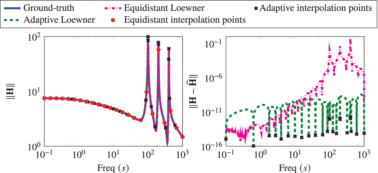
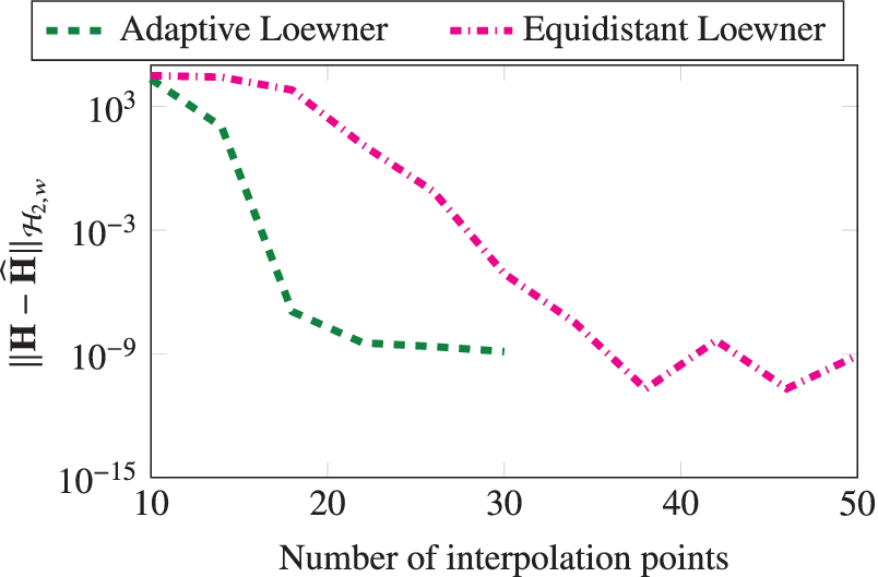
. Using Algorithm 1, we obtain a realization that on termination uses 24 interpolation points. For comparison, we also construct a realization using 24 logarithmically equidistant interpolation points in the given frequency range. We compare these two learned realizations in Figure 2, where we observe that our greedy scheme to collect measurements clearly outperforms the scheme when measurements are taken equidistantly. Algorithm 1 focuses on the region where the transfer function is involved, and it automatically trends to add more points around the peaks of the transfer function. On the other hand, the realization, constructed using the logarithmically equidistant points, has a larger error as it fails to capture these peaks accurately. Furthermore, in Figure 3, we compare the frequency-limited
$ \left[{10}^{-1},{10}^3\right] $
. Using Algorithm 1, we obtain a realization that on termination uses 24 interpolation points. For comparison, we also construct a realization using 24 logarithmically equidistant interpolation points in the given frequency range. We compare these two learned realizations in Figure 2, where we observe that our greedy scheme to collect measurements clearly outperforms the scheme when measurements are taken equidistantly. Algorithm 1 focuses on the region where the transfer function is involved, and it automatically trends to add more points around the peaks of the transfer function. On the other hand, the realization, constructed using the logarithmically equidistant points, has a larger error as it fails to capture these peaks accurately. Furthermore, in Figure 3, we compare the frequency-limited $ {\mathcal{H}}_2 $
-norm (Wilson, Reference Wilson1970) of the learned and ground-truth systems in terms of the number of interpolation points used. We use the MORLAB software package for the computation of the frequency-limited norm (Benner and Werner, Reference Benner and Werner2021). The figure shows that the frequency-limited
$ {\mathcal{H}}_2 $
-norm (Wilson, Reference Wilson1970) of the learned and ground-truth systems in terms of the number of interpolation points used. We use the MORLAB software package for the computation of the frequency-limited norm (Benner and Werner, Reference Benner and Werner2021). The figure shows that the frequency-limited $ {\mathcal{H}}_2 $
error decays faster when the measurements are collected adaptively (Algorithm 1).
$ {\mathcal{H}}_2 $
error decays faster when the measurements are collected adaptively (Algorithm 1).
Penzl example: The Bode plot of the ground-truth, adaptively generated system, and a realization with equidistant points and the corresponding error between them.
Penzl example: A comparison between the frequency-limited $ {\mathcal{H}}_2 $
-norm error for the adaptively chosen points and the equidistant points.
$ {\mathcal{H}}_2 $
-norm error for the adaptively chosen points and the equidistant points.
Next, we compare our method with the IRKA method (Beattie and Gugercin, Reference Beattie and Gugercin2012), as implemented in M-M.E.S.S. (Benner et al., Reference Benner, Köhler, Saak, Benner, Breiten, Faßbender, Hinze, Stykel and Zimmermann2021). We highlight that IRKA aims at determining the optimal interpolation points in the $ {\mathcal{H}}_2 $
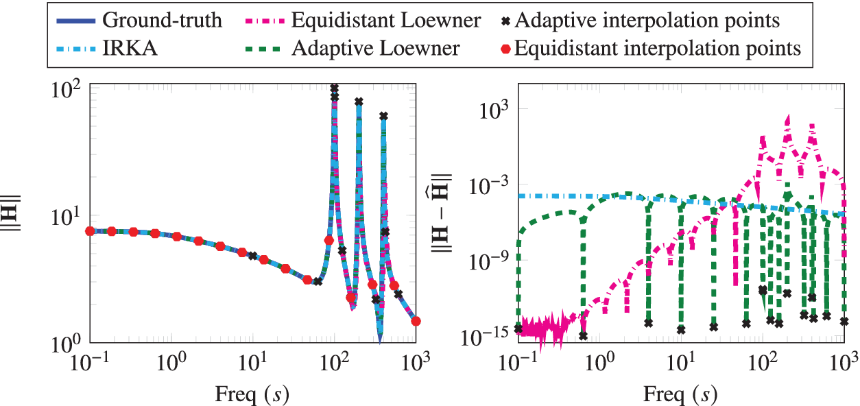
-norm using an iterative scheme, and these interpolation points can be anywhere in the complex domain. This is in contradiction to our proposed method, where we only focus on the imaginary axis due to practical reasoning. We obtain an optimal model of order 16 using IRKA and compare it with the proposed method and the Loewner approach with equidistant points. The results are shown in Figure 4. Although the IRKA method chooses optimal points, the proposed greedy method to construct a realization compares well with IRKA. However, it is quite worthwhile to note that:
$ {\mathcal{H}}_2 $
-norm using an iterative scheme, and these interpolation points can be anywhere in the complex domain. This is in contradiction to our proposed method, where we only focus on the imaginary axis due to practical reasoning. We obtain an optimal model of order 16 using IRKA and compare it with the proposed method and the Loewner approach with equidistant points. The results are shown in Figure 4. Although the IRKA method chooses optimal points, the proposed greedy method to construct a realization compares well with IRKA. However, it is quite worthwhile to note that:
-
(a) IRKA requires the order of the realization as an input which is usually not known.
-
(b) IRKA chooses interpolation points over the whole complex plane but estimating transfer function at these points in an experiment is not straightforward, and sometimes not even possible.
-
(c) Lastly, we highlight that IRKA is an iterative method; hence, it requires repeated evaluations of the transfer function at each iteration. For this example, IRKA took 14 iterations, thus
$ 16\times 14\hskip0.35em =\hskip0.35em 224 $
transfer evaluations. On the other hand, the proposed methodology requires only 16 transfer function evaluations, which are also only on the imaginary axis.

Penzl example: The Bode plots of the ground-truth, adaptively generated system, the realization with equidistant points, and IRKA realization are shown, and the corresponding errors with the ground truth are also presented.
Finally, we study the robustness of Algorithm 1 with respect to the hyperparameter $ \beta $
. We report the quality of the learned realization with respect to the parameter
$ \beta $
. We report the quality of the learned realization with respect to the parameter $ \beta $
in Figure 5. We note that Algorithm 1 is quite robust to the parameter, and all learned realizations outperform the one obtained using the logarithmically equidistant measurement points.
$ \beta $
in Figure 5. We note that Algorithm 1 is quite robust to the parameter, and all learned realizations outperform the one obtained using the logarithmically equidistant measurement points.
Penzl example: A comparison between the resulting Bode plots for different values of $ \beta $
used to defined the filter
$ \beta $
used to defined the filter $ \mathbf{g}\left(\cdot \right) $
in (9).
$ \mathbf{g}\left(\cdot \right) $
in (9).
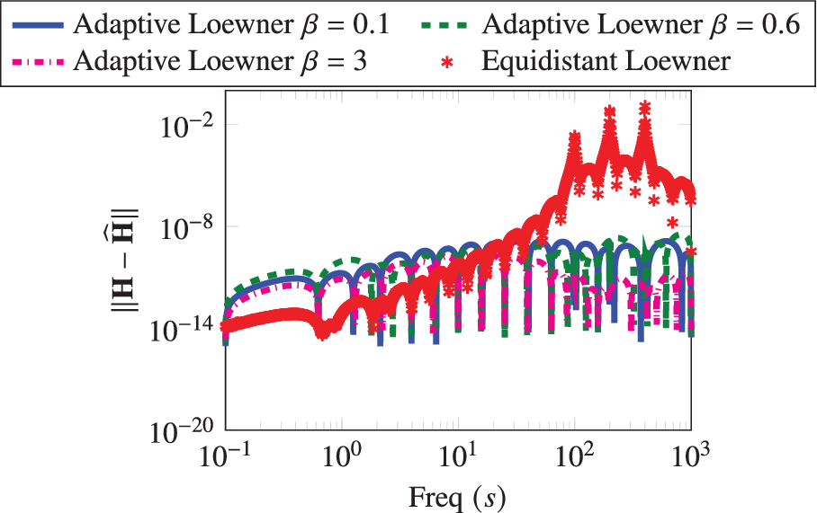
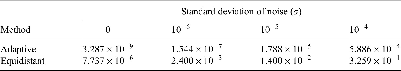
Measurement noise: Many studies have been made about the robustness of the Loewner framework to noise (see, e.g., Lefteriu et al., Reference Lefteriu, Ionita, Antoulas, Willems, Hara, Ohta and Fujioka2010; Kergus et al., Reference Kergus, Formentin, Poussot-Vassal and Demourant2018; Drmač and Peherstorfer, Reference Drmač and Peherstorfer2020). More generally, some studies have worked on designing identification methods that can better deal with noise (see, e.g., Schwerdtner, Reference Schwerdtner2021). We do a preliminary study and observe the performance of our approach under noisy measurements. We conduct three experiments, where we corrupt the transfer function measurements with Gaussian white noise of standard deviation $ \sigma \hskip0.35em =\hskip0.35em \left[{10}^{-4},{10}^{-5},{10}^{-6}\right] $
, respectively. We compare our approach with a realization based on logarithmically equidistant interpolation points and measurements corrupted with the same noise level as for the adaptive case. The
$ \sigma \hskip0.35em =\hskip0.35em \left[{10}^{-4},{10}^{-5},{10}^{-6}\right] $
, respectively. We compare our approach with a realization based on logarithmically equidistant interpolation points and measurements corrupted with the same noise level as for the adaptive case. The $ {\mathcal{H}}_2 $
-norms of learned and the ground-truth models are compared in Table 1. The table shows that even though the
$ {\mathcal{H}}_2 $
-norms of learned and the ground-truth models are compared in Table 1. The table shows that even though the $ {\mathcal{H}}_2 $
error for the adaptive algorithm increases with the level of noise, it yields much better models as compared to the one obtained using the logarithmically equidistant points. This shows that the adaptive method is superior even in the presence of noise in the measurements. It is important to note that the Loewner framework was used to illustrate the application of our method. In the noisy data case, there could be better suitable methods where the proposed adaptive method can be used.
$ {\mathcal{H}}_2 $
error for the adaptive algorithm increases with the level of noise, it yields much better models as compared to the one obtained using the logarithmically equidistant points. This shows that the adaptive method is superior even in the presence of noise in the measurements. It is important to note that the Loewner framework was used to illustrate the application of our method. In the noisy data case, there could be better suitable methods where the proposed adaptive method can be used.
Penzl example: A comparison of the frequency-limited $ {\mathcal{H}}_2 $
-norm of the error between the ground-truth and realized systems under different levels of noise in the measurement data.
$ {\mathcal{H}}_2 $
-norm of the error between the ground-truth and realized systems under different levels of noise in the measurement data.
5.2. Beam example
In this example, we consider the beam model from the SLICOT model reduction library (Chahlaoui and Van Dooren, Reference Chahlaoui and Van Dooren2002). It comes from the discretization of a PDE (Antoulas et al., Reference Antoulas, Sorensen and Gugercin2001). The input is the force applied at one end, and the output is the displacement resulting from the applied force at other end. We consider the frequency range of operation $ \left[{10}^{-1},5\right] $
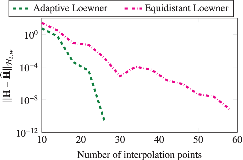
. Algorithm 1 is applied, and a realization is obtained using 30 interpolation points as shown in Figure 6. As in the first example, we also construct a realization using 30 logarithmically equidistant interpolation points distributed over the chosen range of frequencies. Here again, we notice that most of the interpolation points using the adaptive method are chosen around the areas where most changes are happening. In contrast, measurements taken at logarithmically equidistant points yield a realization having a larger error. In Figure 7, we observe that adaptively chosen interpolation points decrease the
$ \left[{10}^{-1},5\right] $
. Algorithm 1 is applied, and a realization is obtained using 30 interpolation points as shown in Figure 6. As in the first example, we also construct a realization using 30 logarithmically equidistant interpolation points distributed over the chosen range of frequencies. Here again, we notice that most of the interpolation points using the adaptive method are chosen around the areas where most changes are happening. In contrast, measurements taken at logarithmically equidistant points yield a realization having a larger error. In Figure 7, we observe that adaptively chosen interpolation points decrease the $ {\mathcal{H}}_2 $
-norm error faster as compared to the equidistant ones.
$ {\mathcal{H}}_2 $
-norm error faster as compared to the equidistant ones.
Beam Example: The Bode plot of the ground-truth system, adaptively generated system, and a realized system with equidistant points. The right figure shows the corresponding error between the ground-truth and realized systems.
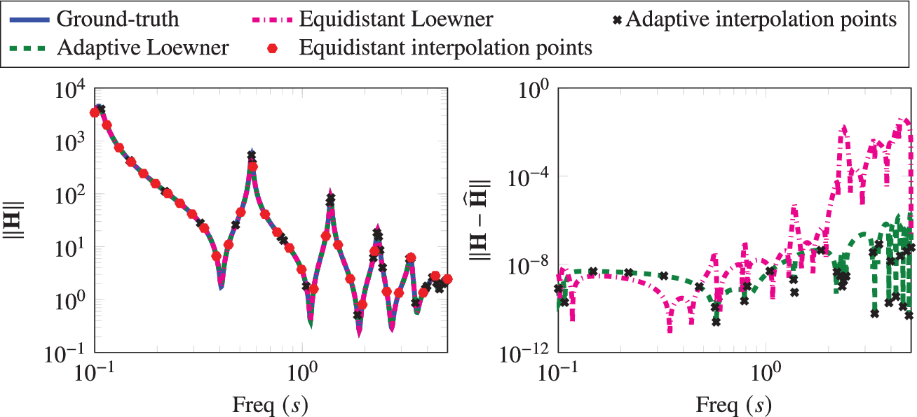
Beam Example: A comparison between the frequency-limited $ {\mathcal{H}}_2 $
norm error for the adaptively chosen points and the equidistant points.
$ {\mathcal{H}}_2 $
norm error for the adaptively chosen points and the equidistant points.
RLC circuit
Finally, we consider an RLC circuit with 100 resistors, capacitors, and inductors (Gugercin and Antoulas, Reference Gugercin and Antoulas2003; Benner et al., Reference Benner, Goyal and Van Dooren2020). The frequencies are taken within the range of frequencies $ \left[{10}^{-2},{10}^3\right] $
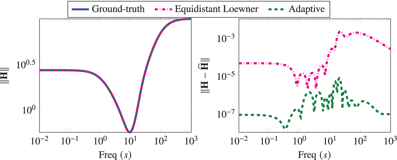
. In order to obtain input/output time-domain measurements, a system simulation using the input (13) is performed to obtain the output in each step. Applying the procedure described in Section 4 directly realizes a model of order 12. As in the first example, we consider the realization of a model using 12 logarithmically equidistant interpolation points and their complex conjugates on the unit circle in order to ensure that the resulting system is real as discussed in Peherstorfer et al. (Reference Peherstorfer, Gugercin and Willcox2017). A comparison of the Bode plots is shown in Figure 8. Our algorithm recovers the model with a relatively low error, and the model captures the time-domain response of the ground-truth model. It shows that our method provides a promising direction for the long-standing subject of input choice for time-domain system identification. In addition, since our method infers only two transfer function measurements in each step, the size of the matrix
$ \left[{10}^{-2},{10}^3\right] $
. In order to obtain input/output time-domain measurements, a system simulation using the input (13) is performed to obtain the output in each step. Applying the procedure described in Section 4 directly realizes a model of order 12. As in the first example, we consider the realization of a model using 12 logarithmically equidistant interpolation points and their complex conjugates on the unit circle in order to ensure that the resulting system is real as discussed in Peherstorfer et al. (Reference Peherstorfer, Gugercin and Willcox2017). A comparison of the Bode plots is shown in Figure 8. Our algorithm recovers the model with a relatively low error, and the model captures the time-domain response of the ground-truth model. It shows that our method provides a promising direction for the long-standing subject of input choice for time-domain system identification. In addition, since our method infers only two transfer function measurements in each step, the size of the matrix $ F $
is small. This results in a more numerically stable optimization problem compared to the classical equidistant selection of points case where you have to solve for all the interpolation at once, leading to the matrix
$ F $
is small. This results in a more numerically stable optimization problem compared to the classical equidistant selection of points case where you have to solve for all the interpolation at once, leading to the matrix $ F $
of large size.
$ F $
of large size.
RLC example: A comparison for the Bode plot of the ground-truth and the identified models.
6. Conclusion
In this paper, we have presented a purely data-driven realization method that greedily chooses measurement points aiming at maximizing the extraction of the information about system dynamics by restricting measurements points on the imaginary axis. We have discussed both cases where data are taken in frequency and time domains. We have illustrated the efficiency of the proposed methodology by means of three benchmark examples. We have shown that our method performs better as compared to the approach where the measurement data are taken at logarithmically equidistant points in a given frequency range. We have observed that the proposed method can learn a good model without prior knowledge about the system dynamics by greedily choosing interpolation points, which is a key advantage.
Data Availability Statement
The source code of the implementations, and the scripts to reproduce the presented results, are available on GitHub under the link https://github.com/mpimd-csc/Greedy_Measurement_Scheme.
Author Contributions
Conceptualization: K.C., P.G., and P.B.; Methodology: K.C., P.G., and P.B.; Software: K.C. and P.G.; Supervision: P.G. and P.B.; Writing—original draft: K.C. and P.G.; Writing—review & editing: K.C., P.G., and P.B. All authors approved the final submitted draft.
Funding Statement
This work received no specific grant from any funding agency, commercial, or not-for-profit sectors.
Acknowledgment
An initial version of the paper is available on arXiv (arXiv:2107.12950) as a preprint (see Cherifi et al., Reference Cherifi, Goyal and Benner2021).
Competing Interests
The authors declare no competing interests exist.


 Open access
Comments
No Comments have been published for this article.