








Impact Statement
This work presents a novel characterization framework for datasets for learning shape optimization problems. It presents an advance in the quantification of dataset diversity that has implications for what data are collected and how the data are generated. While we apply the framework to an automotive aerodynamics problem, the method has broad applicability across engineering optimization.
1. Introduction
The exterior design of an automobile is a result of several considerations, including, among other things, safety, aesthetics, ergonomics, and function. An important concern is the reduction of aerodynamic drag, which, along with rolling resistance from the wheels, is one of two primary contributors to the energy consumption of the vehicle. Numerical prototyping is still an expensive way of design exploration for aerodynamic optimization, however. The complexity of modern vehicle designs leads to a high-dimensional parameter space that can be prohibitively expensive to sample. In addition, the evaluation of the quantity of interest (the drag coefficient) for each single design point is costly, requiring the solution of the Navier–Stokes equations at high Reynolds numbers, on a mesh sufficiently fine so as to resolve the details of configuration, with a model for either all or some of the turbulent scales. Surrogate models are therefore of interest; given the nonlinear nature of the governing equations and the complexity of the geometries of interest, data-driven models for drag prediction are a common choice. The primary issue with constructing surrogates in this application space is the absence of freely-available, realistic automotive geometries, owing primarily to the proprietary nature of commercial designs (see, for instance, the work by the Honda Motor Co. [Nagaoka et al., Reference Nagaoka, Yenerdag, Ambo, Philips, Ivey, Brès and Bose2024], where CFD of several proprietary designs is validated against wind tunnel data).
The two factors that introduce complexity in this specific problem are: first, given the dimension and velocity typical of automotive cruise conditions, the flow regime involves a highly turbulent flow, with a wide range of scales generated. To a first order, assuming homogeneous, isotropic, and fully-developed turbulence, a typical passenger sedan cruising at 70 mph generates turbulent eddies of the order of 10
$ \mu $
 m (Kolmogorov, Reference Kolmogorov1941); this gives about six decades of size separation between the largest and smallest structures in the flow. This turbulence has to be accounted for, either through resolution of the relevant structures using grid and timestep resolution, or through modeling. The second factor is the complexity of automotive geometries (see Figure 1), which require a high surface mesh resolution to capture. Several models for turbulence have been developed for the commonly-used RANS (Reynolds-Averaged Navier–Stokes) approach (Wilcox, Reference Wilcox2006), each with the goal of estimating the impact of the turbulent fluctuations on the time-averaged velocity and pressure fields, which are used to compute the aerodynamic quantities of interest.
Temporal snapshot of time-resolving simulation of flow past a car, showing velocity magnitude contours. Image courtesy: Kun Lu.
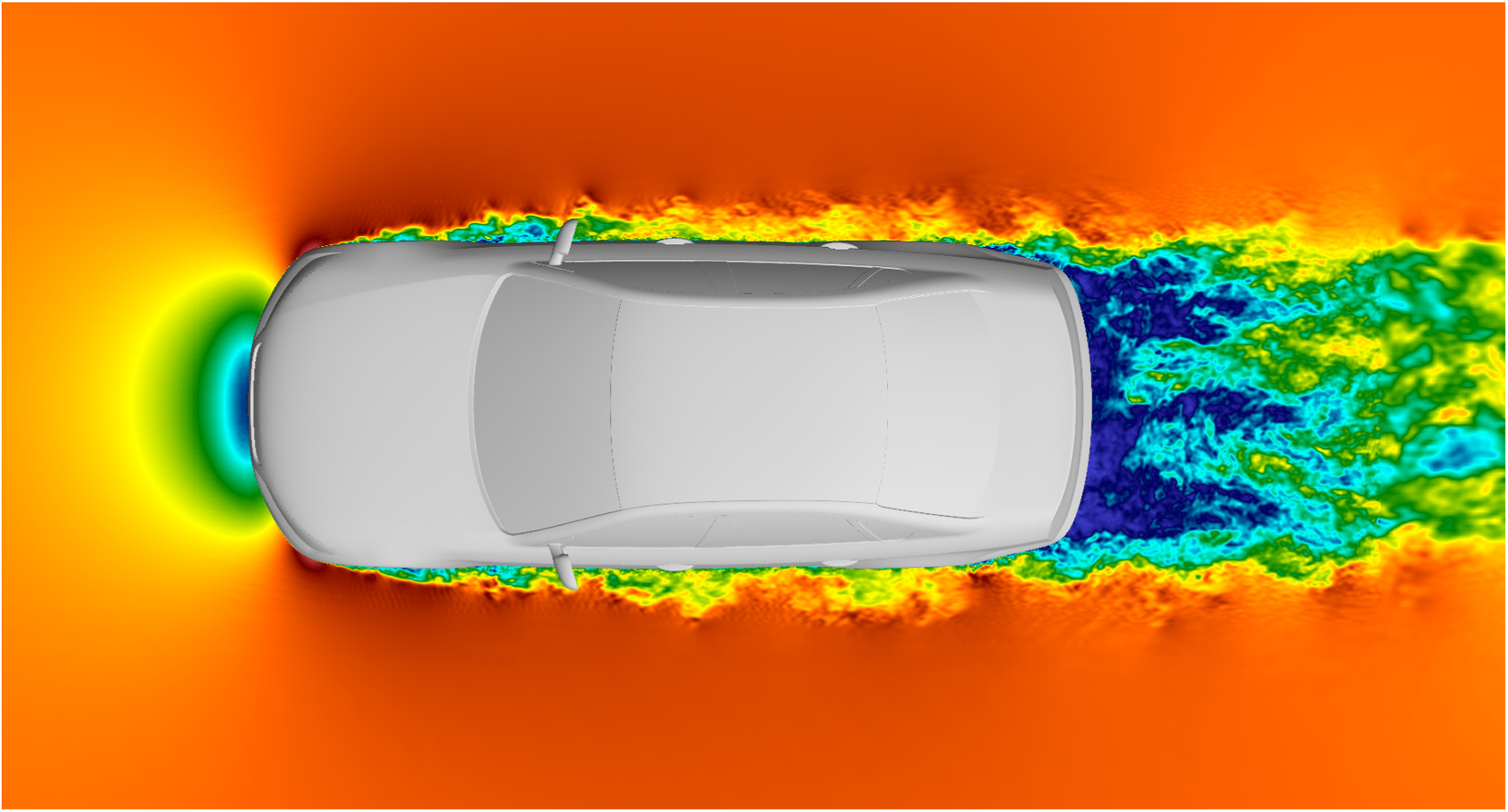
Figure 1. Long description
The visualization uses a color scale where orange represents high velocity and blue represents low velocity. At the West end, a semi-circular stagnation zone of low velocity in green and blue is visible directly in front of the car’s bumper. As the flow moves East along the North and South flanks of the vehicle, thin layers of high-velocity orange air transition into jagged, multicolored turbulent boundary layers. These layers feature a chaotic mix of yellow, green, and cyan. At the East end of the car, a large, wide turbulent wake extends outward. This wake is characterized by a core of deep blue low-velocity pockets interspersed with high-frequency swirls of green and yellow, indicating complex vortex shedding behind the vehicle’s trunk.
One of the first automotive benchmark cases for CFD solvers was the so-called Ahmed Body (Ahmed et al., Reference Ahmed, Ramm and Faltin1984). Over the years, several other configurations have been proposed as reference cases, with varying complexities and parameterizations. A detailed review of the early, simpler models is found in Le Good and Garry (Reference Le Good and Garry2004). A more recent development is the DrivAer model (Heft et al., Reference Heft, Indinger and Adams2012a), a much more detailed and realistic model that has since been the focus of a number of workshops for the evaluation and validation of CFD solvers. With the DrivAer model, it has been found that RANS models struggle to predict the surface pressures accurately even at high resolutions of 300 million cells, and it is found that the scale-resolving Improved Delayed Detached-Eddy Simulations (IDDES) (Shur et al., Reference Shur, Spalart, Strelets and Travin2008; Ashton et al., Reference Ashton, Mockett, Fuchs, Fliessbach, Hetmann, Knacke, Schonwald, Skaperdas, Fotiadis, Walle, Hupertz and Maddix2024) are much better than steady-state calculations (Ashton and Revell, Reference Ashton and Revell2015). With the advancements of computing power, particularly the rise in popularity of graphics processing units (GPUs) for code acceleration, turbulence modeling techniques that capture a portion of the turbulent scales on the grid are becoming more tractable, and it is seen that these methods provide superior accuracy to RANS simulations, particularly in flows with separation (Rodi, Reference Rodi1997).
1.1. Data for learning challenges
There have been attempts in the literature to address the issue of database generation in shape-to-aerodynamics problems. Viquerat and Hachem (Reference Viquerat and Hachem2020) studied the problem of 2D airfoils in the laminar (
$ \mathit{\operatorname{Re}}\hskip0.24em 10 $
 ) regime, and used a random process to generate Bézier curves with which airfoils were developed. Garcia-Fernandez et al. (Reference Garcia-Fernandez, Portal-Porras, Irigaray, Ansa and Fernandez-Gamiz2023) studied simplified representations of heavy vehicles, using CNNs to predict aerodynamic quantities of interest. Other parameterizations explored in the literature is the idea of using a PolyCube map to represent the geometry (Umetani and Bickel, Reference Umetani and Bickel2018), or using parameterized curves to generated two-dimensional silhouettes of cars (Gunpinar et al., Reference Gunpinar, Coskun, Ozsipahi and Gunpinar2019), both of which require manual parameterization, and have been tested on relatively simple shapes. Song et al. (Reference Song, Yuan, Permenter, Arechiga and Ahmed2023) used the versatile ShapeNet database, which is a large repository of freely-available CAD models organized hierarchically, in their investigations of automotive drag. The ShapeNet dataset (Chang et al., Reference Chang, Funkhouser, Guibas, Hanrahan, Huang, Li, Savarese, Savva, Song, Su, Xiao, Yi and Yu2015) has been used in the vast majority of studies to provide training data for machine learning-based aerodynamics predictors (Umetani and Bickel, Reference Umetani and Bickel2018; Rios et al., Reference Rios, Sendhoff, Menzel, Bäck and van Stein2019, Reference Rios, van Stein, Wollstadt, Bäck, Sendhoff and Menzel2021; Remelli et al., Reference Remelli, Lukoianov, Richter, Guillard, Bagautdinov, Baque, Fua, Larochelle, Ranzato, Hadsell, Balcan and Lin2020; Li et al., Reference Li, Kovachki, Choy, Li, Kossaifi, Otta, Nabian, Stadler, Hundt, Azizzadenesheli, Anandkumar, Oh, Naumann, Globerson, Saenko, Hardt and Levine2023; Song et al., Reference Song, Yuan, Permenter, Arechiga and Ahmed2023). The major limitation of ShapeNet is the lack of surface resolution in all of the models, so that the resulting model could not be considered a tool to aid even the initial stages of automotive aerodynamic design.
An approach taken in the literature has been to develop a database with manual parameterizations of the much higher quality DrivAer model discussed earlier (Elrefaie et al., Reference Elrefaie, Dai and Ahmed2024a, Reference Elrefaie, Morar, Dai, Ahmed, Globerson, Mackey, Belgrave, Fan, Paquet, Tomczak and Zhang2024b). For example, Elrefaie et al. (Reference Elrefaie, Dai and Ahmed2024a) generate a database using 29 parameters identified across the entire DrivAer model. The drawbacks to this approach are twofold: first, manual parameterization is labor and time-intensive; second: there is no guarantee that the resulting database is an exhaustive representation of relevant shapes. This approach is thus not scalable beyond limited scope, such as, for example, predicting drag in minor variations of a specific model of automobile.
In this work, we build on the approach introduced by the authors Benjamin and Iaccarino (Reference Benjamin and Iaccarino2025c), henceforth referred to as ShapeCH. Using this approach, it is possible to build a controlled set of database samples using a small number of basis shapes. Using databases generated using this approach, we will address what we term the dataset characterization problem, which can be summarized as follows: there is at present no method to formally make comparisons between different datasets a priori. Table 1 shows a list of currently available datasets for automotive aerodynamics predictions. The majority of databases are derived from either the ShapeNet or DrivAer models, with others using even simpler geometries. However, since these database do not come with a formal characterization of diversity or variety, it is not possible to make any assessments about which database might be suitable for a given application: say, for instance, making predictions on hatchbacks alone. In this case, one might intuitively expect a dataset containing many representative samples of hatchbacks to perform better than one not containing any, but at present there is no way of characterizing this information. Thus, the only way to evaluate different datasets is to train models on them and make predictions, comparing them with any reference drag data that might be available. It is evident that this is not a feasible proceeding in most situations. In the complex realm of automotive design, there is a lack of clarity on the additional coverage in the feature space provided when a new geometry is considered, owing to the nominally high-dimensional parameter space that the designs live in. This also leads to confusion over whether predictions made by models trained on these datasets are actually interpolations or extrapolations.
Datasets for data-driven automotive aerodynamics surrogates
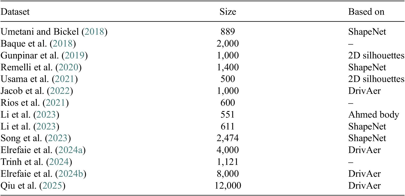
Table 1. Long description
The table consists of three columns: Dataset, Size, and Based on.
* Umetani and Bickel (2018): 889, ShapeNet.
* Baque et al. (2018): 2,000, (no data).
* Gunpinar et al. (2019): 1,000, 2 D silhouettes.
* Remelli et al. (2020): 1,400, ShapeNet.
* Usama et al. (2021): 500, 2 D silhouettes.
* Jacob et al. (2021): 1,000, DrivAer.
* Rios et al. (2021): 600, (no data).
* Li et al. (2023): 551, Ahmed body.
* Li et al. (2023): 611, ShapeNet.
* Song et al. (2023): 2,474, ShapeNet.
* Elrefaie et al. (2024): 4,000, DrivAer.
* Trinh et al. (2024): 1,121, (no data).
* Elrefaie et al. (2024): 8,000, DrivAer.
* Qiu et al. (2025): 12,000, DrivAer.
1.2. Learning automotive aerodynamics from data
Several approaches have been taken in the literature to develop neural network-based models for automotive aerodynamics.
Planar projections of the automobile can be used, these views can be flattened by applying developable transformations to them (Benjamin et al., Reference Benjamin, Saetta, Ivey, Bose, Ham and Iaccarino2023); these representations can be parsed by CNNs (Song et al., Reference Song, Yuan, Permenter, Arechiga and Ahmed2023). The images can contain information about depth of field, as well as surface normals. The two main drawbacks of this approach are the forced uniform resolution of the pixelization over all regions of the image (which has been somewhat, but not completely solved by feature pyramid approaches [Lin et al., Reference Lin, Dollár, Girshick, He, Hariharan and Belongie2017]) and the problem of occlusion in nonconvex shapes. The latter problem is application specific; occlusion is a more significant issue when the geometry of interest has several internal structures (such as the internal cooling passages in a turbomachinery blade) than in exterior automotive surfaces, for examples. A possible solution is to utilize several slices through the geometry, rather than just one. An extension of CNNs to three dimensions, with 3D convolutions operating on voxel grids, is possible but not desirable due to computing and storage requirements scaling cubically with the characteristic length scale resolved by the voxel (Maturana and Scherer, Reference Maturana and Scherer2015).
Another common representation of a surface is a point cloud, which is simply an unordered set of vectors that contain coordinate information. The format is simple and low storage compared to three-dimensional voxelizations, and PointNets have been developed as an architecture class uniquely suited to working with point clouds (Qi et al., Reference Qi, Su, Mo and Guibas2017a). The key to working with point clouds is to ensure invariance of the functions in the network to permutations of the vectors in the set, and the PointNet architecture achieves this using a symmetric max pooling function. Subsequent iterations of the architecture (Qi et al., Reference Qi, Yi, Su, Guibas, Guyon, von Luxburg, Bengio, Wallach, Fergus, Vishwanathan and Garnett2017b) use hierarchical feature extraction to compensate for the lack of connectivity information in the point clouds. Owing to their innate hierarchical construction, CNNs tend to generalize better than PointNets. Surface tessellations or meshes are a popular representation choice, and MeshCNNs (Hanocka et al., Reference Hanocka, Hertz, Fish, Giryes, Fleishman and Cohen-Or2019) operate directly on meshes, using edges as the basis element to apply convolutions. MeshCNNs are tailored to work with triangular tessellations, and see applications in segmentation tasks for 3D models. For a more flexible approach, the connectivity information in meshes can be assembled into graphs. Graph neural networks (GNNs) are designed to take advantage of this format (Wu et al., Reference Wu, Pan, Chen, Long, Zhang and Yu2021), using message passing to aggregate information from neighboring nodes. A development that enables the use of convolutions are the Graph Convolutional Networks (GCNs) (Kipf and Welling, Reference Kipf and Welling2017). While GCNs handle spatial locality more naturally than PointNets, they can be difficult to train. In addition, they are much more sensitive to perturbations to the graph connectivity than PointNets. Scalability is also a concern with GCNs for large graphs. Combinations of the earlier architecture types have been developed more recently, such as the Point–Voxel CNN architecture (Liu et al., Reference Liu, Tang, Lin and Han2019), which combines the benefits of PointNets and VoxelNets, and Regularized Graph Convolutional Neural Networks (RGCNNs) (Te et al., Reference Te, Hu, Guo and Zheng2018), which are a combination of point cloud representations with graph neural networks. Another recent development is the Geometry-Informed Neural Operator (GINO) (Li et al., Reference Li, Kovachki, Choy, Li, Kossaifi, Otta, Nabian, Stadler, Hundt, Azizzadenesheli, Anandkumar, Oh, Naumann, Globerson, Saenko, Hardt and Levine2023), which is a hybrid architecture that combines GNNs and Fourier Neural Operators (FNOs) (Li et al., Reference Li, Kovachki, Azizzadenesheli, Liu, Bhattacharya, Stuart and Anandkumar2020). A summary of the earlier representation types and the corresponding network architectures is shown in Table 2.
Surface representations and corresponding network types
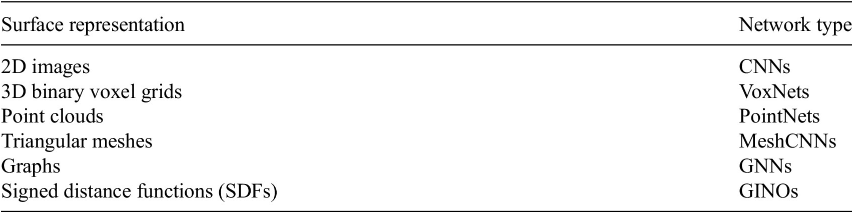
Table 2. Long description
The table consists of two columns titled Surface representation and Network type.
* Row 1: 2 D images correspond to C N N s.
* Row 2: 3 D binary voxel grids correspond to VoxNets.
* Row 3: Point clouds correspond to PointNets.
* Row 4: Triangular meshes correspond to Mesh C N N s.
* Row 5: Graphs correspond to G N N s.
* Row 6: Signed distance functions, abbreviated as S D F s, correspond to G I N O s.
The database generation procedure introduced in this work has the benefit of being compatible with any of the network architectures listed ealier, and the choice of specific representations and corresponding network types is made with a view to make predictions with accuracy suitable for the datasets under consideration, not to present a comparative analysis of different architectures. The focus of the work is solely on the dataset construction.
In a previous work by Benjamin and Iaccarino (Reference Benjamin and Iaccarino2025c), a methodology is developed for generating geometries for training in a controlled manner, starting with a small number of starting cases. Using the database developed in that work, we develop a measure of diversity that can be used to characterize different datasets.
2. Database generation, simulation, and model training
2.1. Database generation using ShapeCH
ShapeCH is a procedure that uses a limited number of starting (or basis) geometries that form a convex hull (CH) in the space of 3D shapes. From these basis configurations, intermediate geometries are developed by shape interpolation of the corresponding Signed Distance Function (SDF). The methodology is described in detail in Benjamin and Iaccarino (Reference Benjamin and Iaccarino2025c), but we provide a succinct summary here: first, the basis STL tessellations are converted into SDFs using structured ray-tracing along orthogonal axes. Rays cast from bounding box faces detect surface intersections via the Moller–Trumbore algorithm, creating binary voxel grids (BVGs). The distance transform of the BVGs yields continuous SDF representations where positive values indicate interior regions and negative values exterior space. Then, barycentric interpolation is performed within the convex hull of the basis geometries. Given
$ n $
 input SDFs
$ {\phi}_i^p $
input SDFs
$ {\phi}_i^p $
 , interpolated shapes are computed as
$ {\overline{\phi}}_i(d)={\sum}_{p=1}^n{w}_p{\phi}_i^p(d) $
, interpolated shapes are computed as
$ {\overline{\phi}}_i(d)={\sum}_{p=1}^n{w}_p{\phi}_i^p(d) $
 subject to
$ \sum {w}_p=1 $
subject to
$ \sum {w}_p=1 $
 and
$ {w}_p\ge 0 $
and
$ {w}_p\ge 0 $
 . This weighted combination preserves topological features while enabling smooth morphing between basis configurations. Finally, zero-level sets are extracted from interpolated SDFs and triangulated surfaces are reconstructed using the marching cubes algorithm. In addition to the automotive aerodynamics application in the original work by Benjamin and Iaccarino (Reference Benjamin and Iaccarino2025c), the work has been used in generating datasets for wind loading predictions on buildings (Vargiemezis et al., Reference Vargiemezis, Kanatsoulis and Gorlé2025).
2.2. Geometry and the DrivAerCH3 database
To best represent the complexities of a realistic automobile, we consider the DrivAer model discussed earlier, an open-source midsize passenger car geometry developed to assess the quality and contrast automotive aerodynamics investigations carried out using computational fluid dynamics tools (Aultman et al., Reference Aultman, Wang, Auza-Gutierrez and Duan2022). The model is available in three configurations: a fastback, estate, and sedan, shown in Figure 2.
DrivAer back configurations: estateback (left), fastback (center), and notchback (right).
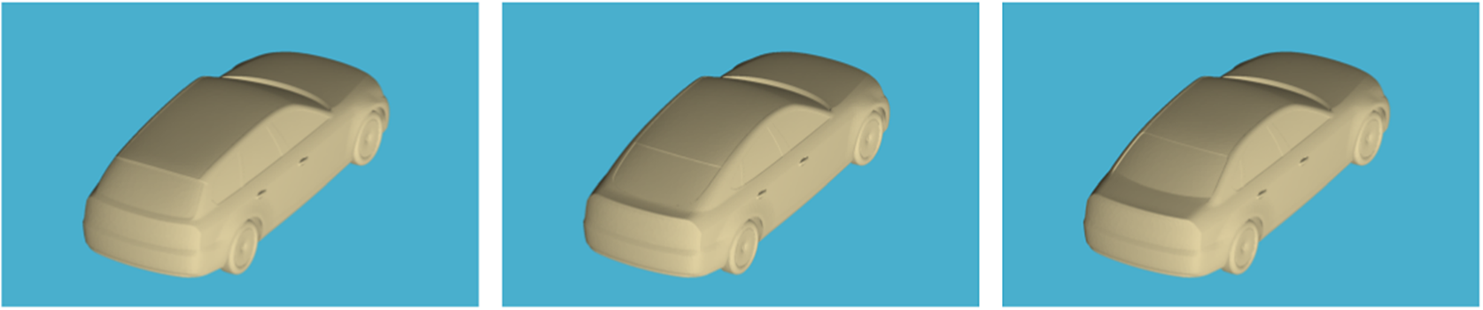
We construct the dataset by using the three back configurations of the DrivAer model as the basis elements of the convex hull (Benjamin and Iaccarino, Reference Benjamin and Iaccarino2025c). The identifier applied to this dataset is “DrivAerCH3,” where the “CH3” represents that the convex hull is generated from three basis geometries (a triangle in 2D). In general, with
$ n $
 basis geometries we construct a simplex in
$ n-1 $
basis geometries we construct a simplex in
$ n-1 $
 dimensions. Note that no other user-specified input is required to generate infinite new configurations by sampling in the SDF space. The three configurations are different enough so as to provide a sufficient variation in drag coefficient (the separation aft of the vehicle being significantly impacted by the form of the rear roof slope), but also similar enough to provide a controlled testing ground for the proposed methodology.
2.3. From a database to a dataset: large eddy simulations
Large eddy simulations (LES) are used to obtain the ground truth aerodynamic quantities of interest for the training dataset. Large eddy simulations directly resolve the largest, energy-containing scales of turbulent flows, and model the smallest scales. This is achieved by the application of a low-pass filter to the governing Navier–Stokes equations of motion, whereby scales smaller than the filter are removed. In common practice, high-frequency modes are removed implicitly by a combination of the finite sizing of the mesh and the filtering effect of numerical discretization of the equations.
LES simulations are carried out at fixed speed (85 mph) and without wheel rotation, using the CharLES solver. Details of the Voronoi diagram-based meshing paradigm used in the tool can be found in Brès et al. (Reference Brès, Bose, Emory, Ham, Schmidt, Rigas and Colonius2018), and the formulation of the low-Mach Helmholtz pressure solver is outlined in Ambo et al. (Reference Ambo, Nagaoka, Philips, Ivey, Brès and Bose2020). The code has been validated in aerodynamics analysis of a number of high-Reynolds number flow studies (Goc et al., Reference Goc, Lehmkuhl, Park, Bose and Moin2021). The current simulations use ~2 million control volumes, with refinement near the surfaces of the car as shown in Figure 3. The mesh resolution on the surface is
$ \Delta /L=0.0023 $
 , where
$ \Delta $
, where
$ \Delta $
 is the local mesh size and
$ L $
is the local mesh size and
$ L $
 is the characteristic length of the car. The domain is sized at
$ 15L\times 8L\times 6L $
is the characteristic length of the car. The domain is sized at
$ 15L\times 8L\times 6L $
 , with the car placed at
$ 5L $
, with the car placed at
$ 5L $
 from the inlet. Since the Helmholtz formulation permits low-frequency pressure oscillations, we use a numerical sponge at
$ 2L $
from the inlet. Since the Helmholtz formulation permits low-frequency pressure oscillations, we use a numerical sponge at
$ 2L $
 from the domain boundaries to reduce the time for the reflecting waves to be damped out. The Vreman subgrid model is used to approximate the effects of the subgrid scales on the resolved scales, and walls are modeled using the algebraic wall model. The flow is initialized with a converged initial condition from the baseline DrivAer notchback geometry. The simulation is run for a total time of 2 seconds, and statistics are collected for the last 1 second. The simulation parameters are summarized in Table 3. We choose to limit our experiments to static wheels for the following two reasons: first, while wheel rotation is important to capture absolute count variations in drag, and important in industrial settings, we are simply concerned with a representative dataset where drag “delta” (the difference in drag between different simulations) is represented with sufficient accuracy so as to demonstrate our dataset generation and characterization framework; second, it has been shown in Nagaoka et al. (Reference Nagaoka, Yenerdag, Ambo, Philips, Ivey, Brès and Bose2024) that moving mesh simulations of wheels provide significant accuracy gains for automotive simulations compared to other methods such as rotating boundary conditions, chiefly owing to the non-axisymmetric nature of the wheel rims. However, the moving mesh simulations were too expensive for the computational budget of this study, due to the large number of geometries simulated. Hence, we confine our attention to simulations with no wheel rotations.
View of the mesh used for the large eddy simulations, with refinement zones shown: (a) near the car, (b) in the wake. (c) Instantaneous velocity magnitude contours showing wake behind the car.
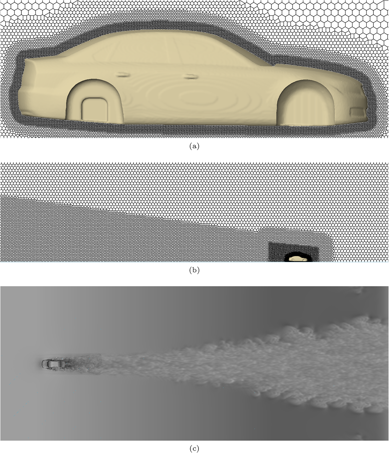
Figure 3. Long description
A three-panel vertical stack labeled a, b, and c.
Panel a shows a side profile of a tan sedan within a computational mesh. The mesh density is highest immediately adjacent to the car body, appearing as a dark, solid band of extremely fine cells. Moving outward, the mesh transitions into a medium-density layer before becoming a coarse, large-scale hexagonal grid at the perimeter.
Panel b provides a wider view of the mesh refinement zones. The car is a small silhouette in the bottom right. A dense, wedge-shaped refinement zone extends from the rear of the car toward the left, representing the wake region. The surrounding area consists of a uniform, medium-coarse hexagonal mesh.
Panel c displays a grayscale contour plot of instantaneous velocity magnitude. The car is positioned on the left, and a turbulent, plume-like wake extends horizontally to the right. The wake is characterized by complex, swirling eddies and varying shades of gray, indicating fluctuating velocity gradients behind the vehicle.
Simulation setup details for the DrivAerCH3 database
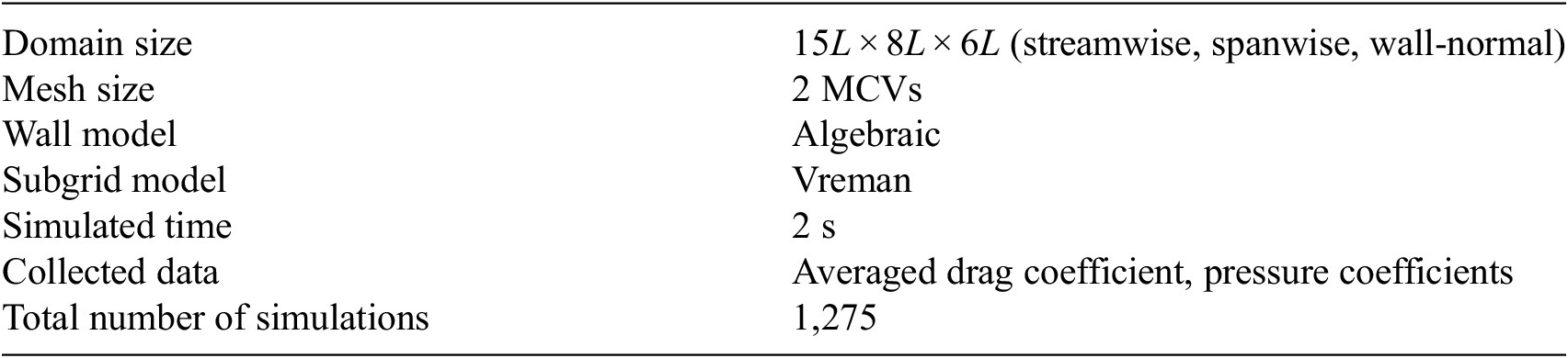
Table 3. Long description
The table consists of two columns: Parameter and Value.
* Domain size: 15 L times 8 L times 6 L (streamwise, spanwise, wall-normal).
* Mesh size: 2 M C V s.
* Wall model: Algebraic.
* Subgrid model: Vreman.
* Simulated time: 2 s.
* Collected data: Averaged drag coefficient, pressure coefficients.
* Total number of simulations: 1,275.
The main output of interest for this study is the drag coefficient, computed as
$ {C}_d=2{F}_d/\rho {v}^2A $
 , where
$ {F}_d $
, where
$ {F}_d $
 is the drag force,
$ \rho $
is the drag force,
$ \rho $
 is the fluid density,
$ v $
is the fluid density,
$ v $
 is the freestream flow velocity, and
$ A $
is the freestream flow velocity, and
$ A $
 is the frontal area of the car projected in the direction of the flow.
The wall time for a single simulation is about 12 minutes on a NVIDIA H100 GPU (Choquette, Reference Choquette2023). We make comparisons with the original set of experiments carried out by Heft et al. (Reference Heft, Indinger and Adams2012b). The configuration that matches the one that we use is the Fastback, with the smooth underbody, without mirrors, with wheels (the F_S_woM_wW experiment from Figure 9 of Heft et al.). The reported
$ {C}_D $
 in that case is 0.227, which compares well with our value of 0.223. Our LES predictions match the experiments better than the Heft et al. RANS simulations which give a value of 0.233. We construct a refined grid of 4M CVs and verify that the difference between the two grids is less than 1% at the pixel resolution used for the CNNs (see Figure 4). We note that the experiments in the article were at a lower Reynolds number than ours (
$ 7M $
in that case is 0.227, which compares well with our value of 0.223. Our LES predictions match the experiments better than the Heft et al. RANS simulations which give a value of 0.233. We construct a refined grid of 4M CVs and verify that the difference between the two grids is less than 1% at the pixel resolution used for the CNNs (see Figure 4). We note that the experiments in the article were at a lower Reynolds number than ours (
$ 7M $
 vs.
$ 10M $
vs.
$ 10M $
 ), however, the
$ {C}_D $
), however, the
$ {C}_D $
 is observed to plateau around that Reynolds number, so we do not believe this has a significant impact. The selected Reynolds number is chosen to correspond with typical highway speed limits.
Planar images of the left view of the notchback, showing (left) the normalized surface pressure coefficient computed on the 2M CV grid, (center) the normalized surface pressure coefficient computed on the 4M CV grid, and (right) the relative error between the two solutions.
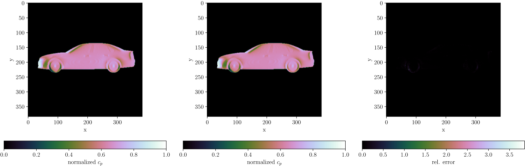
Figure 4. Long description
A three-panel set of planar plots on a black background. Each plot uses an x-axis from 0 to 350 and a y-axis from 0 to 350 to map the left side of a notchback vehicle.
* The left panel displays the normalized c sub p computed on a 2 M C V grid. The car body is primarily pink, indicating values around 0.6 to 0.7, with green highlights near the front bumper and wheel wells. A color bar below ranges from 0.0 (black) to 1.0 (white).
* The center panel displays the normalized c sub p computed on a 4 M C V grid. The visual distribution of pressure is nearly identical to the first panel, with the same pink and green color mapping and a 0.0 to 1.0 scale.
* The right panel displays the relative error between the 2 M and 4 M solutions. The car silhouette is almost entirely black, indicating very low error across the surface. Faint purple highlights are visible only at the edges of the wheels and the very front of the bumper. The color bar below ranges from 0.0 to 3.5.
2.4. Model architecture
We use the image-based representation and convolutional neural network model (U-net) architectures found in Benjamin and Iaccarino (Reference Benjamin and Iaccarino2025c). The inputs to the model are three planar projects of the geometry: the back, the side, and the top (shown in Figure 5), stacked to make three channels. The image resolution is
$ 384\times 384 $
 , which is chosen to match the resolution of the mesh cells of the CFD and the resolution of the ray tracing. This choice is done in keeping with the need to resolve sufficiently fine changes to the surface. Concretely, taking the different discretization choices (ray tracing, mesh, and image resolution) into account, a geometry modification of about 12 mm to a surface can be detected in a vehicle that is 4 m long. The data in the images are binned into 255 bits.
Planar images of the normal distance from the camera (top row) and the normalized surface pressure coefficients (bottom rows) for a sample DrivAer geometry. The input images with the check marks (and the corresponding output views) are used for training.
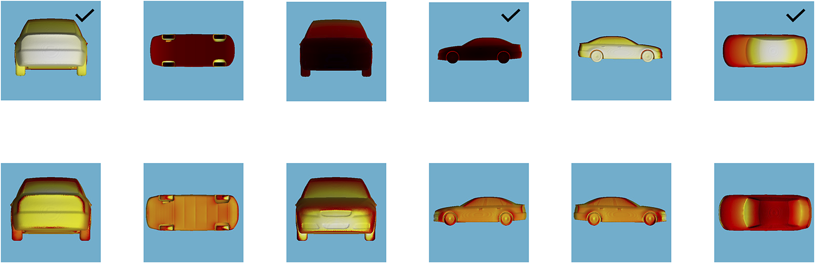
Figure 5. Long description
The grid consists of two rows and six columns.
Top Row: Displays normal distance from the camera.
- Panel 1: Rear view with a check mark in the top right corner.
- Panel 2: Bottom view showing the undercarriage.
- Panel 3: Front view.
- Panel 4: Side profile view with a check mark in the top right corner.
- Panel 5: Three-quarter side view.
- Panel 6: Top-down view with a check mark in the top right corner.
Bottom Row: Displays normalized surface pressure coefficients corresponding to the views above.
- Panel 7: Rear view showing pressure distribution.
- Panel 8: Bottom view.
- Panel 9: Front view.
- Panel 10: Side profile view.
- Panel 11: Three-quarter side view.
- Panel 12: Top-down view.
Color gradients indicate varying values, with the top row using a dark-to-light scale and the bottom row using a red-to-yellow heat map scale.
Figure 6 shows a selection of samples from the dataset. One can see how the roofline is gradually morphed to produce designs intermediate to the basis cases. It is also evident how regions of low pressure are more apparent in the more estate-like designs, which is a result of the larger separation bubble that design tends to produce. With this method of generating training samples, the parameterization is not tied to discrete design features such as the door mirrors or handles (Benjamin et al., Reference Benjamin, Saetta, Ivey, Bose, Ham and Iaccarino2023), but a comprehensive three-dimensional morphological operation, designed to provide a high density of data point clustering in feature space.
Surface pressure coefficients (
$ {c}_p $
 ) shown on left side views of a selection of samples in dataset, showing a transition from the notchback (top left) to the estateback (bottom right), with the fastback visited along the way. Values are normalized between 0 and 255 per sample.
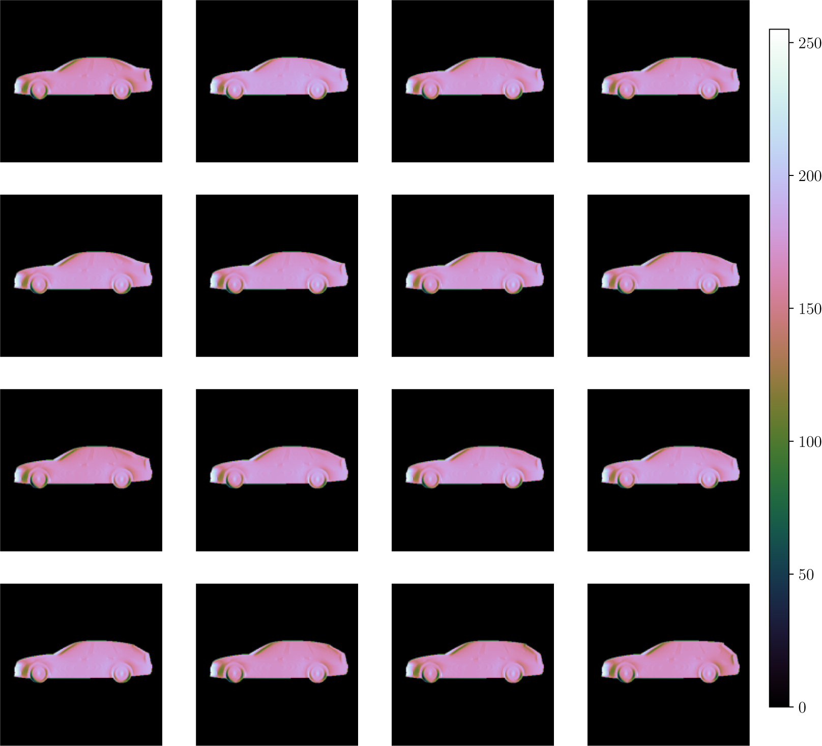
Figure 6. Long description
A four-by-four grid of sixteen panels displays side-view silhouettes of cars against a black background. Each car is color-mapped to represent surface pressure coefficients, C sub p.
* The sequence begins at the top-left with a notchback design, characterized by a distinct three-box shape with a clear horizontal trunk line.
* Moving through the grid from left to right and top to bottom, the rear roofline gradually elongates and flattens.
* The middle panels show fastback variations where the roof slopes continuously to the rear bumper.
* The sequence concludes at the bottom-right with an estateback or station wagon design, featuring a long, high roofline that extends to the rear of the vehicle.
On the far right, a vertical color scale bar ranges from 0 at the bottom to 250 at the top. The color gradient transitions from black at 0, through dark blue, green, and yellow, to pink and white at 250. The car surfaces are predominantly pink, indicating high-pressure values, with small areas of green and blue concentrated around the wheels and lower bumpers, indicating lower pressure regions.
Schematic of U-Net architecture for the
$ {c}_p $
 model.
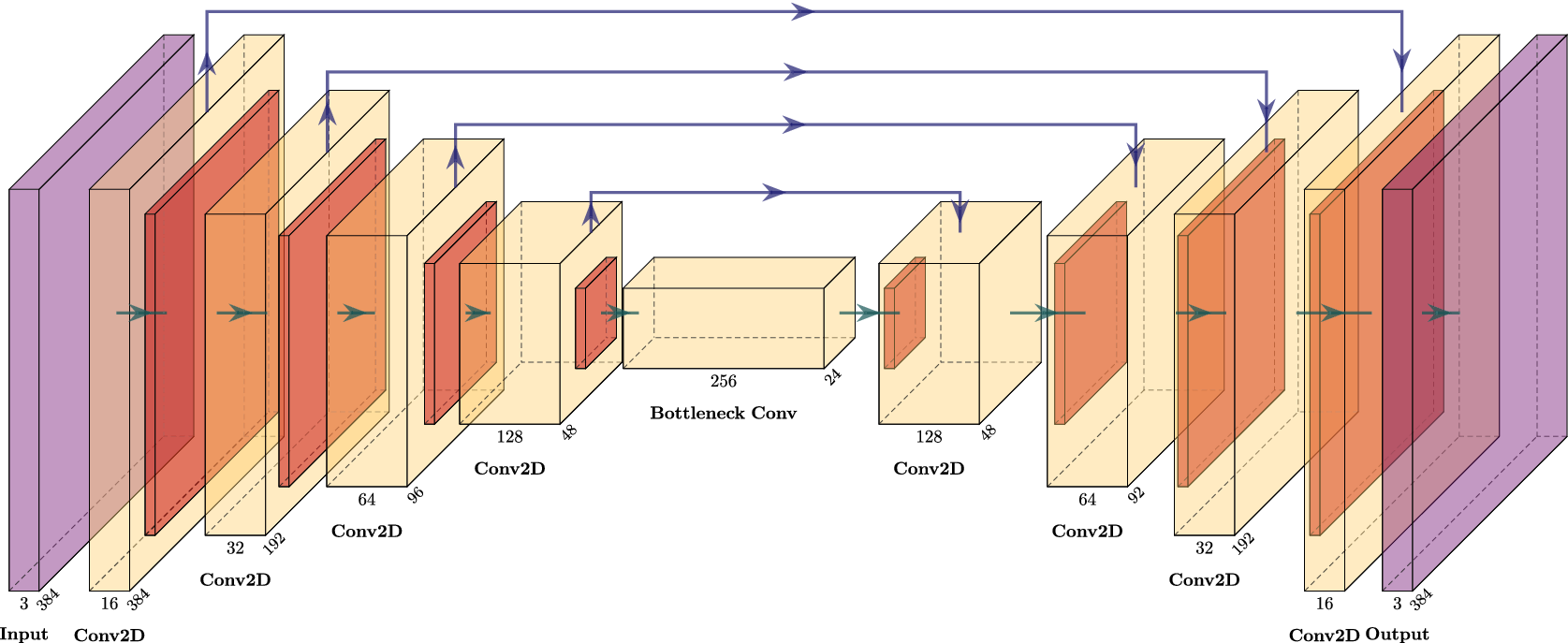
Figure 7. Long description
The diagram illustrates a U-shaped neural network.
* Contracting Path (Left): Begins with an Input layer of size 3 by 384. It descends through four Conv 2 D blocks. The first block is 16 by 384, the second is 32 by 192, the third is 64 by 96, and the fourth is 128 by 48. Each block is represented by a series of overlapping colored rectangular prisms (purple, yellow, and red).
* Bottleneck (Center): A horizontal rectangular prism labeled Bottleneck Conv with dimensions 256 by 24.
* Expansive Path (Right): Ascends through four corresponding Conv 2 D blocks that mirror the left side. It starts at 128 by 48, moves to 64 by 92, then 32 by 192, and finally 16 by 384, ending at a Conv 2 D Output of 3 by 384.
* Skip Connections: Four blue horizontal arrows originate from the top of each Conv 2 D block on the contracting side and point directly to the corresponding block on the expansive side, bypassing the bottleneck.
* Data Flow: Green horizontal arrows indicate the sequential processing between adjacent blocks within the contracting and expansive paths.
The U-Net downsamples the input (dimension
$ 384\times 384\times 3 $
 ) to a bottleneck of
$ 24\times 24\times 256 $
) to a bottleneck of
$ 24\times 24\times 256 $
 (Figure 7). The hyperparameters (learning rate, filters per layer, and optimizer type) are tuned by grid search. Architecture details are in Table 4. For a full review of the results of the DrivAerCH3 model, we refer the reader to the ShapeCH paper (Benjamin and Iaccarino, Reference Benjamin and Iaccarino2025c).
Network architecture
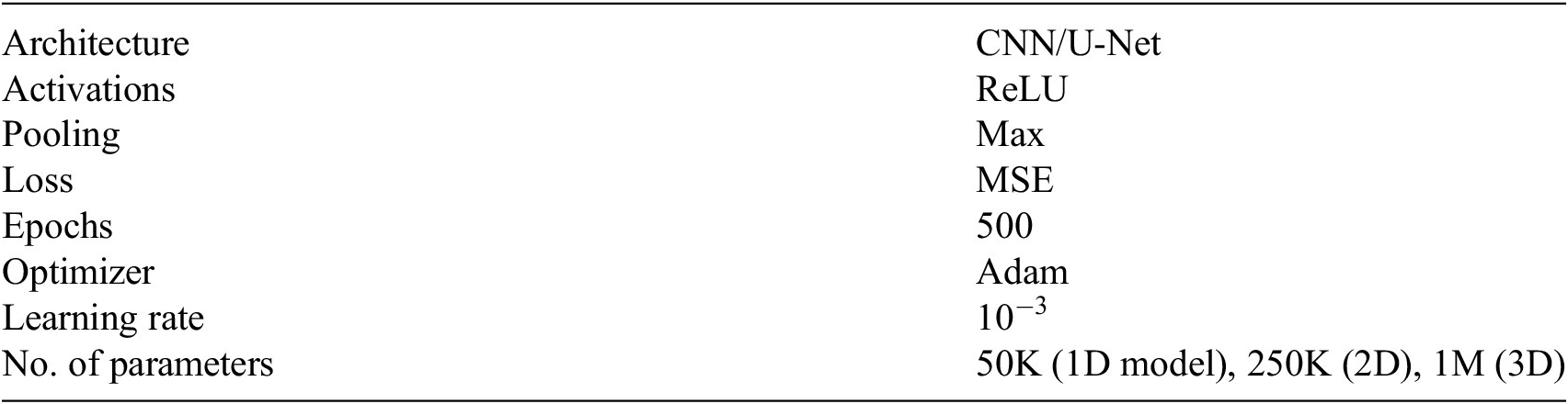
Table 4. Long description
The table consists of two columns: Architecture and Specification.
* Architecture: C N N / U-Net
* Activations: R e L U
* Pooling: Max
* Loss: M S E
* Epochs: 500
* Optimizer: Adam
* Learning rate: 10 super minus 3
* No. of parameters: 50 K for the 1 D model, 250 K for the 2 D model, and 1 M for the 3 D model.
3. Dataset characterization
With the background for the datasets in place, we now focus on the topic of dataset diversity. This is of critical importance in the current application, given the extremely high number of parameters requires to describe typical automotive shapes. The question we address is simply this: given two datasets A and B of identical size, how would one determine which dataset is better? Traditionally, attributes used to describe datasets have an emphasis on the quality of individual data points, providing quantification of statistical bias, correlation, or experimental noise (Brazdil et al., Reference Brazdil, van Rijn, Soares, Vanschoren, Brazdil, van Rijn, Soares and Vanschoren2022). However, if all the datasets under consideration are from a single, sufficiently reliable origin, such metrics are likely to be fairly uniform across all of them. The goal of dataset characterization under such conditions is to provide a measure of how well the underlying problem domain (i.e., the space of possible geometrical configurations) is represented. If one seeks a universal predictor of aerodynamic drag for automobiles under given flow conditions, dataset characterization should assist in the selection of the dataset that provides most coverage of the feature space. Assuming that factors such as the dataset size, data quality, distribution of target values, and variability in input features are the same, one would like to distinguish between a dataset with only minor variations of a certain type of vehicle, and one with many different vehicle types represented. It can be argued that with access to an infinitely large database, it would be possible to achieve a true universal prediction, but in practical terms there is either scarcity of data or cost constraints that require a decision of how to select data for learning. In the following, we formalize these notions and ultimately derive an empirical scaling law that quantifies how prediction error depends on both diversity and dataset size. We propose to characterize dataset using three features:
-
1. Size: The number of samples in the dataset. A larger size is correlated with better generalizability and reduced overfitting of the model to the training data. Deep networks empirically perform better when trained on datasets of large size (LeCun et al., Reference LeCun, Bengio and Hinton2015).
-
2. Density: The number of samples per region of feature space. In $ {\mathrm{\mathbb{R}}}^1 $
 , this reduces to the number of samples per unit length. A higher concentration of samples improves interpolative capabilities. The concept of density is aligned closely to the idea of granularity in computer vision applications (Cui et al., Reference Cui, Gu, Mahajan, van der Maaten, Belongie and Lim2019). In general, in the absence of control over the data-sampling process, density can be different in different regions of the input space.
 -
3. Diversity: A measure of the variety of the feature space, reducing to the span in $ {\mathrm{\mathbb{R}}}^1 $
. Higher diversity can aid with generalization by exposing the model to a broader range of inputs, reducing bias toward specific subsets of the inputs.


An illustrative example in
$ {\mathrm{\mathbb{R}}}^1 $
 is shown in Figure 8, for training data collected from an underlying sinusoidal signal. It is seen that two of the three characteristics change simultaneously whenever a change to the dataset is made. This example also shows how diversity can be thought of as improving the representation of the underlying truth in the training set.
Illustration of size, density, and diversity of a dataset in
$ {\mathrm{\mathbb{R}}}^1 $
 . Crosses represent training samples. Gray solid line represents the underlying truth. (a) Baseline; (b) same diversity, but different size and density; (c) same density, but different size and diversity; (d) same size, but different diversity and density.
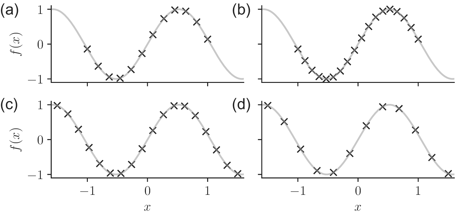
Figure 8. Long description
A four-panel set of line graphs labeled a through d. Each graph shares the same axes where the horizontal x-axis ranges from negative 1 to 1 and the vertical y-axis f of x ranges from negative 1 to 1. A solid gray cosine wave represents the ground truth in all panels. Black crosses represent training samples.
Panel a, top-left, shows a baseline distribution with samples concentrated between x equals negative 1 and positive 1.
Panel b, top-right, shows the same diversity as panel a but with higher density, featuring more crosses packed closely along the same segment of the curve.
Panel c, bottom-left, shows the same density as panel a but higher diversity, with crosses spread further along the x-axis to cover the full visible range of the wave.
Panel d, bottom-right, shows the same sample size as panel a but with lower density and higher diversity, resulting in crosses that are widely spaced apart across the entire horizontal range.
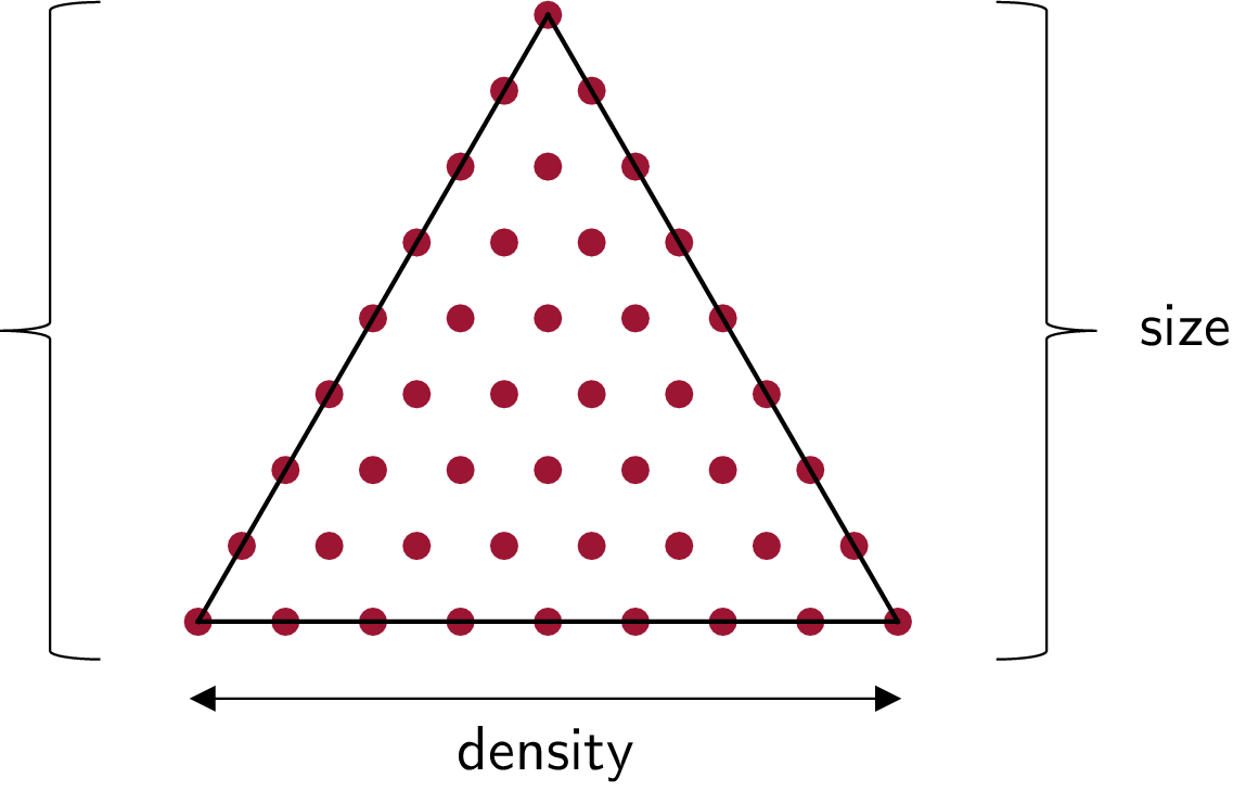
ShapeCH allows for a natural definition of the earlier characteristics. The size of the dataset is trivially defined as the total number of samples drawn in the convex hull. The density is defined as the number of samples per dimension of the simplex (see Figure 9). There are alternate ways to define this quantity: for instance, one could use the inverse of the average volume of the Voronoi cell containing the sample. This could be a subject of future study, particularly in the context of nonuniform sampling. Additional nuance may be added to this definition when more complex forms of high-dimensional sampling are used. The diversity of the dataset is correlated to two disparate effects: the dimensionality of the simplex, and the variety in the basis cases. As an illustration, one might generate a more diverse training set by moving from a
$ p $
 - to a
$ \left(p+1\right) $
- to a
$ \left(p+1\right) $
 -dimensional simplex by adding a new basis case. One could also affect the diversity by staying with a
$ p $
-dimensional simplex by adding a new basis case. One could also affect the diversity by staying with a
$ p $
 -dimensional simplex, but replacing one of the basis cases with a geometry that is more “different” by some measure than the existing case, leading to more variety in the interpolated shapes.
Illustration of database size and density in the ShapeCH framework.
3.1. A metric for diversity
In devising a metric for diversity, the following properties are desirable:
-
• The metric should be a non-negative scalar for a given dataset.
-
• The metric should be higher for more diverse datasets.
-
• The metric should be independent of the units or scale of the problem (i.e., invariant under uniform scaling of geometry and domain).
-
• The metric should be independent of the dimension of the simplex.
-
• The metric should be sensitive to affine dependence in the basis cases; that is, if one of the corners of the barycentric triangle was obtained by taking an affine combination of the other corners, the diversity metric should reduce. A subset of this condition is that if one of the corners is directly replaced with one of the others, the diversity metric should reduce as well.
It is evident that STL representations of geometries or surface meshes for simulations are not easy to work with when it comes to making assessments of differences between two cases, because the unstructured tessellation is not straightforward to standardize. However, the SDFs are an ideal representation with which to make point-to-point comparisons. Thus, given the above requirements, the following metric is proposed: given
$ n $
 discrete SDFs (i.e., basis configurations),
$ {\phi}_1,{\phi}_2,\dots, {\phi}_n\in {\unicode{x211D}}^{N_x\times {N}_y\times {N}_z} $
discrete SDFs (i.e., basis configurations),
$ {\phi}_1,{\phi}_2,\dots, {\phi}_n\in {\unicode{x211D}}^{N_x\times {N}_y\times {N}_z} $
 , the pairwise L-2 distance between two SDFs
$ {\phi}_p $
, the pairwise L-2 distance between two SDFs
$ {\phi}_p $
 and
$ {\phi}_q $
and
$ {\phi}_q $
 is computed as

The pairwise distance matrix
$ D $
 is constructed where
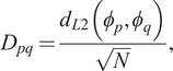
where
$ N $
 is the total number of points in the voxel grid.
To obtain a scalar diversity metric, the off-diagonal elements of the distance matrix are averaged:
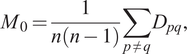
where
$ n $
 is the number of basis SDFs (i.e.,
$ n=p+1 $
is the number of basis SDFs (i.e.,
$ n=p+1 $
 , with
$ p $
, with
$ p $
 the simplex dimension). To ensure that the metric is scale independent (i.e., invariant to uniform scaling of the geometry and domain), the final diversity metric is normalized by the box length
$ {L}_{\mathrm{box}} $
the simplex dimension). To ensure that the metric is scale independent (i.e., invariant to uniform scaling of the geometry and domain), the final diversity metric is normalized by the box length
$ {L}_{\mathrm{box}} $
 :
:

Combining the earlier steps,
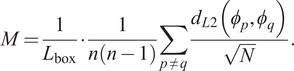
It is noted here that the metric is a comparative one; the numerical value obtained from a dataset only makes sense when compared against the value obtained from another dataset; the one with the higher value has higher diversity. The development of diversity metrics of this kind is seen in the functional ecology literature (Mammola et al., Reference Mammola, Carmona, Guillerme and Cardoso2021) to enable quantification of the extent of trait differences across different species of plant or animal. It is important to emphasize that the diversity of the databases generated using ShapeCH depends only on the basis cases.
To validate the metric, it is first applied to simple geometric databases.
As a simple model problem, consider the database generated from the convex hull of a unit sphere, a unit cube, and a unit right cone. The centroids of the shapes are aligned, and their SDFs obtained by ray tracing at a resolution of
$ {32}^3 $
 . The diversity metric
$ M $
. The diversity metric
$ M $
 is computed for a variety of configurations, and the values shown in Table 5. A baseline value of
$ 1.83\times {10}^{-6} $
is computed for a variety of configurations, and the values shown in Table 5. A baseline value of
$ 1.83\times {10}^{-6} $
 is obtained for the value of
$ M $
is obtained for the value of
$ M $
 . When the right cone is replaced by an ellipsoid with major and minor axes half-lengths of 1 and 0.5, respectively,
$ M $
. When the right cone is replaced by an ellipsoid with major and minor axes half-lengths of 1 and 0.5, respectively,
$ M $
 drops to
$ 1.77\times {10}^{-6} $
drops to
$ 1.77\times {10}^{-6} $
 , which is consistent with our expectation that the convex hull of these three shapes is smaller, and therefore less diverse, than the convex hull including the cone. Likewise, when there is duplication of the sphere in the basis set, we see that the metric falls even further: a duplicated element lies at the centroid of the pair, minimizing its contribution to diversity. And finally, a basis set containing the same sphere repeated returns a diversity metric of 0, as expected.
Diversity metric for model databases
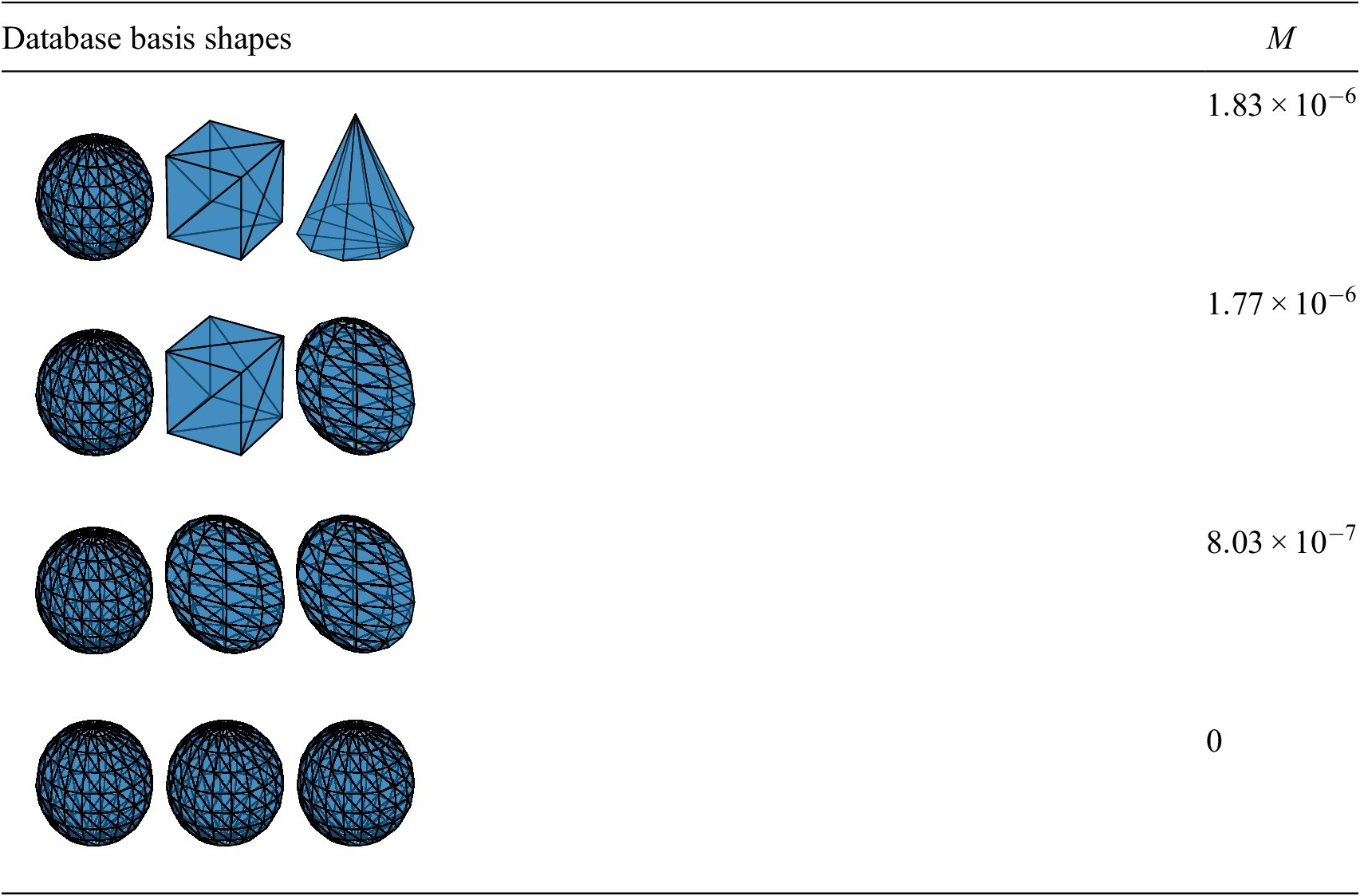
Table 5. Long description
The table consists of two columns titled Database basis shapes and M.
* Row 1: The shape is a collection of diverse 3D objects including a chair, a table, and various abstract geometric forms. The value for M is 1.83 times 10 super minus 6.
* Row 2: The shape is a set of four distinct chairs with varying backrest and leg designs. The value for M is 1.77 times 10 super minus 6.
* Row 3: The shape is a set of four identical chairs. The value for M is 8.03 times 10 super minus 7.
* Row 4: The shape is a single chair. The value for M is 0.
A footnote indicates that all S D F s are computed at 32 super 3 resolution.
Note. All SDFs are computed at
$ {32}^3 $
 resolution.
As a second validation, consider three spheres with tessellations of varying refinement: the first has 2,400 triangles, the second 32,000, and the third 240,000. The three shapes nominally represent the same object, but are subject to a small surface discretization error due to faceting. For a dataset generated with these bases, we expect the diversity metric to be small, yet nonzero. Accordingly, the metric is computed to be
$ 1.3\times {10}^{-9} $
 , which is very small. The value is computed for a ray-tracing resolution of
$ {256}^3 $
, which is very small. The value is computed for a ray-tracing resolution of
$ {256}^3 $
 rays, and changes slightly to
$ 1.34\times {10}^{-9} $
rays, and changes slightly to
$ 1.34\times {10}^{-9} $
 for
$ {512}^3 $
for
$ {512}^3 $
 rays, due to an interaction of the approximations introduced by the tessellation and the ray tracing.
3.2. A hierarchy of datasets
To demonstrate the effects of varying diversities and to prepare the ground for a quantitative scaling law relating diversity to prediction error, a hierarchy of datasets is constructed, with an increasing number of basis cases. The number of samples is kept approximately constant. Thus, in the higher dimensional datasets, the diversity increases, while the density decreases, as the number of points per dimension of the simplex decreases. A total of six basis cases is considered: the first three are the variations of the DrivAer model from the previous sections, the next three are configurations of the AeroSUV model (Zhang et al., Reference Zhang, Tanneberger, Kuthada, Wittmeier, Wiedemann and Nies2019), developed to be an SUV (Sports Utility Vehicle) equivalent to the DrivAer. Figure 10 shows how the three SUV models compare against the sedan. The wheelbase of both the SUV and sedan being identical ensures that the intermediate geometries have the same wheel assemblies; in general, this would not be true for arbitrary basis cases. However, the method is not conditioned on the interpolated shapes having a certain degree of verisimilitude; any shapes generated will still be used to “teach” the neural network about the drag response, providing a useful data point.
The six basis STLs used in generating the datasets. Left column: DrivAer models; right column: equivalent AeroSUV models.
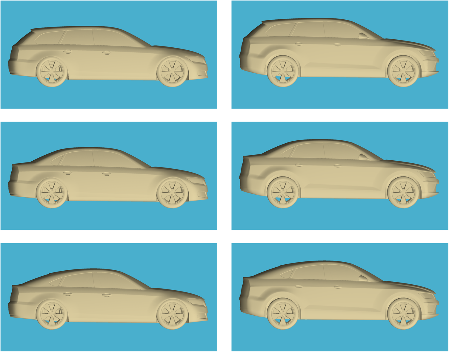
The basis cases that make up each dataset are detailed next. Each dataset comprised approximately 750 samples; for each dataset, the density (or number of samples per dimension of the simplex) is chosen to be the value that results in the dataset size being closest to 750 for a uniform, full-factorial sampling. For convenience, each dataset is named after the polygon that has a number of sides corresponding to the number of basis cases.
-
1. The DrivAerCH3 dataset: This dataset is generated from a 2D simplex using the DrivAer estateback, fastback, and notchback as basis cases.
-
2. The DrivAerCH4 dataset: This dataset is generated from a 3D simplex using the DrivAer estateback, fastback, notchback, and AeroSUV estateback as basis cases.
-
3. The DrivAerCH5 dataset: This dataset is generated from a 4D simplex using the DrivAer estateback, fastback, notchback, AeroSUV estateback, and fastback as basis cases.
-
4. The DrivAerCH6 dataset: This dataset is generated from a 5D simplex using the DrivAer estateback, fastback, notchback, AeroSUV estateback, fastback, and notchback as basis cases.
The details of the earlier datasets can be found in Table 6. With the samples generated, LES is performed of all cases under identical conditions as discussed earlier, taking 1330 H100 core-hours in total. As one might expect, there is a significant increase in the range of the drag coefficient with the addition of the SUV model. Figure 11 shows the distribution of
$ {C}_D $
 values for each of the four datasets. The first dataset, which has the same diversity as the original dataset (but a lower density and size), has a much narrower range of values, and the diversity in the output space increases as the diversity of the dataset increases.
Datasets’ characteristics
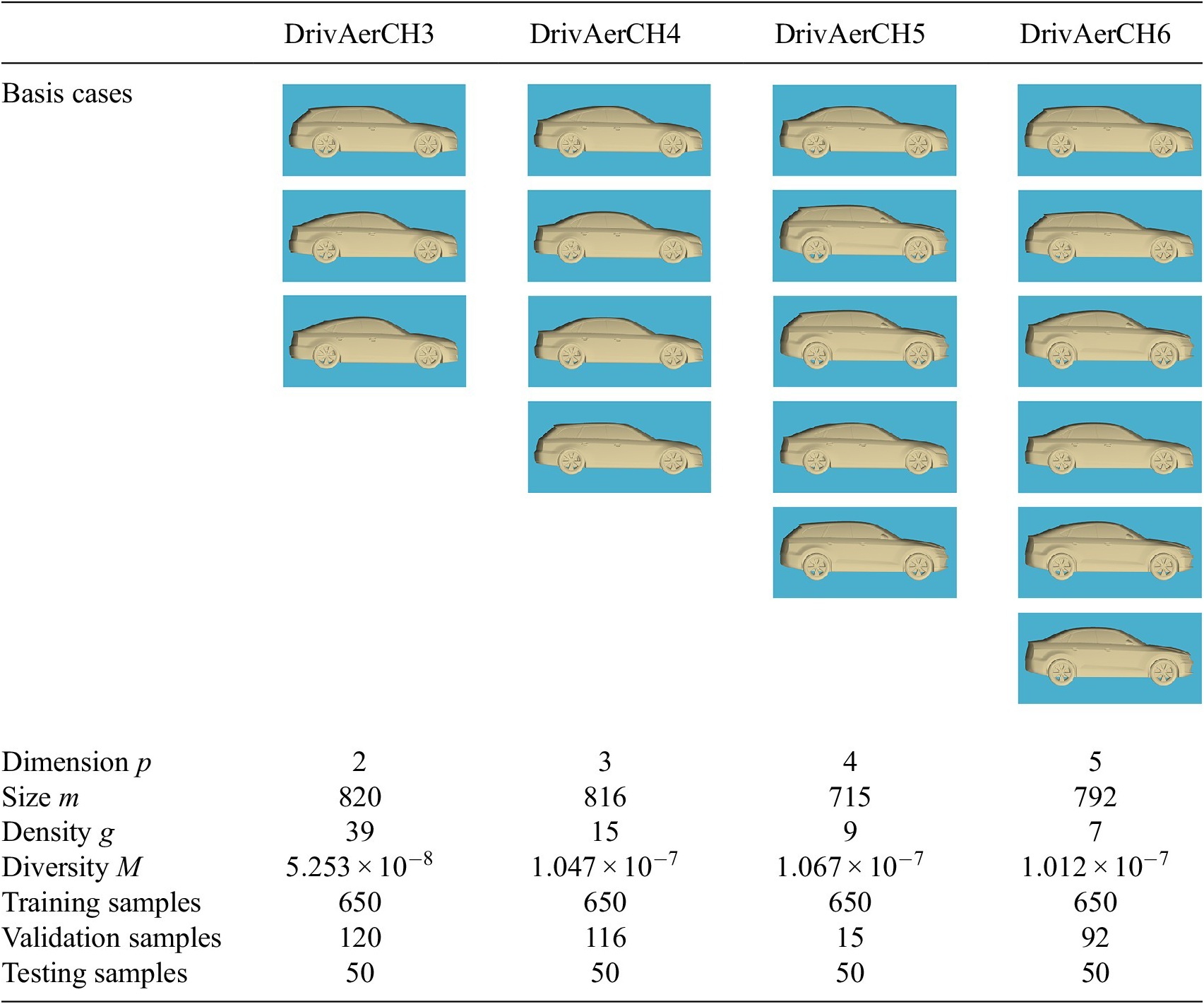
Table 6. Long description
The table is organized into four columns for datasets DrivAerCH3, DrivAerCH4, DrivAerCH5, and DrivAerCH6.
* Basis cases: Shown as a series of car profile images. DrivAerCH3 has 3 images; DrivAerCH4 has 4 images; DrivAerCH5 has 5 images; and DrivAerCH6 has 6 images.
* Dimension p: Values are 2, 3, 4, and 5 respectively.
* Size m: Values are 820, 816, 715, and 792 respectively.
* Density g: Values are 39, 15, 9, and 7 respectively.
* Diversity M:
- DrivAerCH3: 5.253 times 10 super minus 8.
- DrivAerCH4: 1.047 times 10 super minus 7.
- DrivAerCH5: 1.067 times 10 super minus 7.
- DrivAerCH6: 1.012 times 10 super minus 7.
* Training samples: All datasets have 650.
* Validation samples: Values are 120, 116, 15, and 92 respectively.
* Testing samples: All datasets have 50.
Histograms of drag coefficients of different datasets. Left to right: the DrivAerCH3 dataset, the DrivAerCH4 dataset, the DrivAerCH5 dataset, and the DrivAerCH6 dataset.
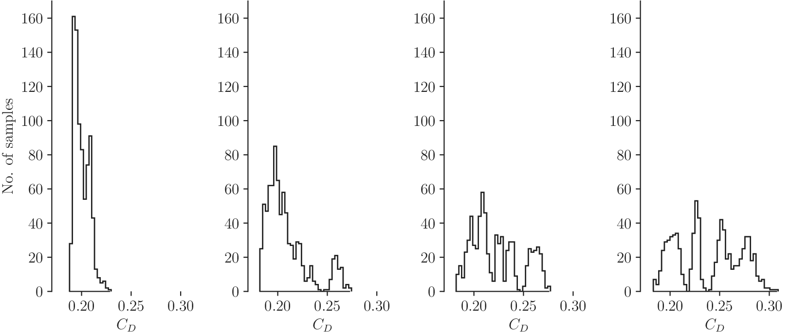
Figure 11. Long description
A multi-panel figure containing four histograms. All panels share a vertical y-axis labeled No. of samples ranging from 0 to 160 and a horizontal x-axis labeled C sub D ranging from 0.20 to 0.30.
* The first panel on the left, representing the DrivAerCH3 dataset, shows a highly concentrated, narrow peak centered around 0.20 with a maximum frequency of approximately 160 samples.
* The second panel, representing the DrivAerCH4 dataset, shows a broader distribution with a primary peak near 0.20 reaching about 85 samples and a smaller secondary peak near 0.26.
* The third panel, representing the DrivAerCH5 dataset, displays a multi-modal distribution with several lower peaks. The highest peak is around 0.21 with approximately 60 samples, and the data is spread more evenly between 0.18 and 0.27.
* The fourth panel on the right, representing the DrivAerCH6 dataset, shows the widest distribution. It features multiple distinct peaks of similar height, roughly 40 to 55 samples, spanning across the range from 0.18 to 0.30.
While DrivAerCH3 provides us with a convenient barycentric triangle, the higher dimensional simplices of the DrivAerCH4 through the DrivAerCH6 datasets are more difficult to visualize. As an aid to dataset interpretation, we employ the multidimensional scaling (MDS) (Cox and Cox, Reference Cox and Cox2000) technique to project the datasets down to two dimensions. MDS preserves the distances between different samples (in these cases, the distances are given naturally by the interpolation weights), in the lower dimensional space. Figures 12–15 show the MDS projections of the DrivAerCH3, DrivAerCH4, DrivAerCH5, and DrivAerCH6 datasets, respectively. Each sample is colored by the drag coefficient obtained from the LES. The drag coefficient is not used in defining similarity between samples; the distances are based on the feature space.
Multidimensional scaling (MDS) of the DrivAerCH3 dataset. Each sample is colored by drag coefficient obtained from LES. Silhouettes indicate the basis samples.
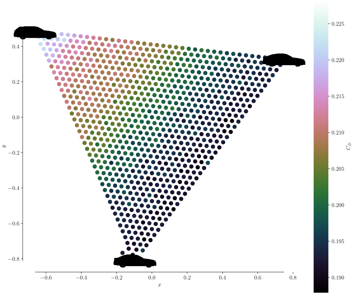
Figure 12. Long description
A scatter plot on a Cartesian coordinate system with x and y axes ranging from negative 0.8 to 0.8. The data points form a large triangular distribution. Three black car silhouettes act as spatial anchors at the vertices. One silhouette is at the top-left, one at the top-right, and one at the bottom-center.
On the right side, a vertical color bar represents the drag coefficient C sub D, ranging from 0.190 at the bottom (dark black-blue) to 0.225 at the top (light cyan).
Data trends within the triangle:
* The top-left region near the first silhouette contains light purple and pink dots, indicating C sub D values around 0.215 to 0.220.
* The top-right region near the second silhouette contains dark navy and black dots, indicating the lowest C sub D values near 0.190.
* The bottom vertex near the third silhouette also contains dark navy dots.
* The center of the triangle shows a gradient transition through olive green and brown hues, representing mid-range drag coefficients between 0.205 and 0.210.
DrivAerCH4 dataset. See Figure 12 for details.
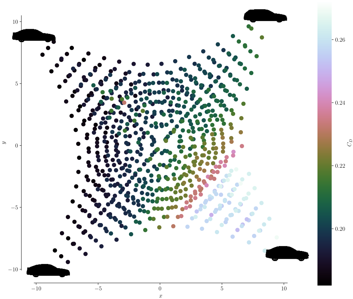
Figure 13. Long description
The scatter plot uses a Cartesian coordinate system where the x-axis and y-axis both range from negative 10 to 10. At the center of the plot, data points are arranged in concentric circular patterns. As the distance from the origin increases, the points transition into four distinct diagonal arms extending toward the corners of the plot.
Each corner is anchored by a black silhouette of a car model.
* Top-left corner: A hatchback silhouette.
* Top-right corner: An S U V silhouette.
* Bottom-left corner: A sedan silhouette.
* Bottom-right corner: A fastback silhouette.
A vertical color bar on the right represents the drag coefficient, C sub D, ranging from 0.18 at the bottom to 0.27 at the top. The color gradient transitions from black at the bottom, through dark green, olive, pink, and light purple, to light cyan at the top.
Data distribution by color:
* The left side and center-left regions are dominated by dark blue and black points, indicating lower C sub D values around 0.18 to 0.20.
* The center-right and top-right regions feature olive and dark green points, representing mid-range C sub D values around 0.22 to 0.23.
* The bottom-right quadrant contains a cluster of light cyan and pale purple points, indicating the highest C sub D values exceeding 0.26.
DrivAerCH5 dataset. See Figure 12 for details.
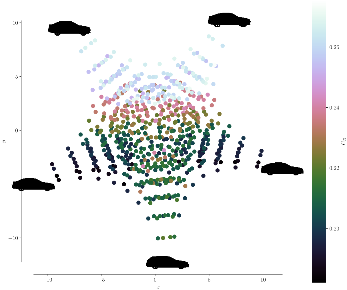
Figure 14. Long description
A scatter plot with x and y axes ranging from negative 10 to 10. The data points are arranged in a fan-like or pentagonal distribution. A vertical color bar on the right represents the drag coefficient C sub D, ranging from 0.18 at the bottom in black to 0.27 at the top in light cyan.
* The bottom-most points at x equals 0 and y equals negative 10 are dark green, corresponding to a station wagon silhouette.
* Moving upward toward the center, the density of points increases, showing a mix of dark green and dark blue colors.
* At the center of the plot, points transition into olive and pink hues.
* The top-left region contains light blue and lavender points, corresponding to a notchback car silhouette.
* The top-right region contains the lightest cyan points, corresponding to a fastback car silhouette.
* The far-left and far-right mid-sections feature dark blue and black points, corresponding to two different sedan silhouettes.
* The overall trend shows higher C sub D values concentrated at the top of the plot and lower values at the bottom and sides.
DrivAerCH6 dataset. See Figure 12 for details.
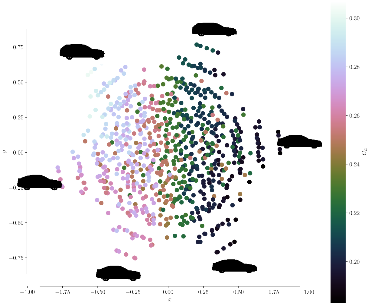
Figure 15. Long description
A scatter plot with x and y axes ranging from negative 1.00 to 1.00. The data points are densely clustered in a circular formation around the origin. A vertical color bar on the right represents the drag coefficient C sub D, ranging from 0.18 at the bottom in black to 0.30 at the top in light cyan. The color gradient transitions from black to dark green, olive, pink, light purple, and finally cyan.
Six black car silhouettes are positioned around the perimeter of the central cluster to illustrate the vehicle types at different coordinate extremes:
* Top-left: A large S U V silhouette.
* Top-center: A smaller hatchback silhouette.
* Middle-right: A sedan silhouette with a prominent rear spoiler.
* Bottom-right: A standard sedan silhouette.
* Bottom-center: A different sedan profile.
* Middle-left: A large S U V silhouette similar to the top-left.
The data points within the cluster are color-coded according to the C sub D scale, showing a concentration of lower drag values (darker colors) on the right side of the plot and higher drag values (lighter purple and cyan) on the left side.
4. Results
4.1. Network performance
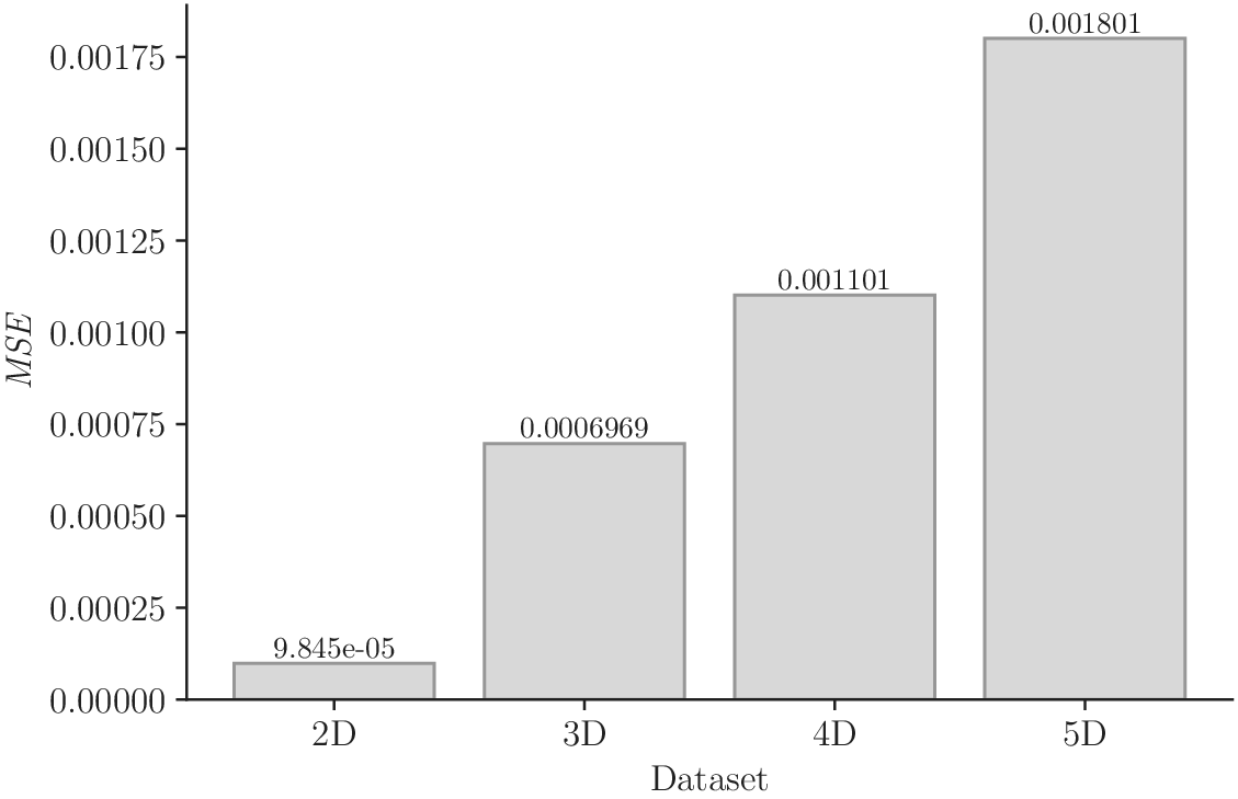
As the diversity of a training dataset grows (and its density decreases), given a fixed size, one expects to see an impact on the performance of models trained on DrivAerCH3 versus DrivAerCH6. The performance of the models in predicting the drag coefficients is shown in Figure 16. As the diversity of the datasets increases, the accuracy drops; more data are required to learn the increased variety in the training set. The reduced density of sampling leads to degraded interpolative performance.
Mean absolute error in drag counts for CNNs trained on different datasets when predicting the aerodynamic drag. Left to right: DrivAerCH3, DrivAerCH4, DrivAerCH5, and DrivAerCH6.
The U-Nets are also used to make surface pressure predictions on the four datasets. Figure 17 shows the prediction of one sample from the test set from each of the models. A similar inverse correlation with diversity and accuracy is seen. The model trained on the DrivAerCH3 dataset reconstructs the fine details of the low-pressure zones created by the vortices released from the roofline–rear window junction (Heft et al., Reference Heft, Indinger and Adams2012b); this accurate representation gradually degrades until there is almost no fine-grained structure left in the predictions of the model trained on the most diverse DrivAerCH6 dataset.
Surface pressure coefficient
$ {c}_p $
 predictions for models trained on DrivAerCH3 (first row), DrivAerCH4 (second row), DrivAerCH5 (third row), and DrivAerCH6 (fourth row), respectively.
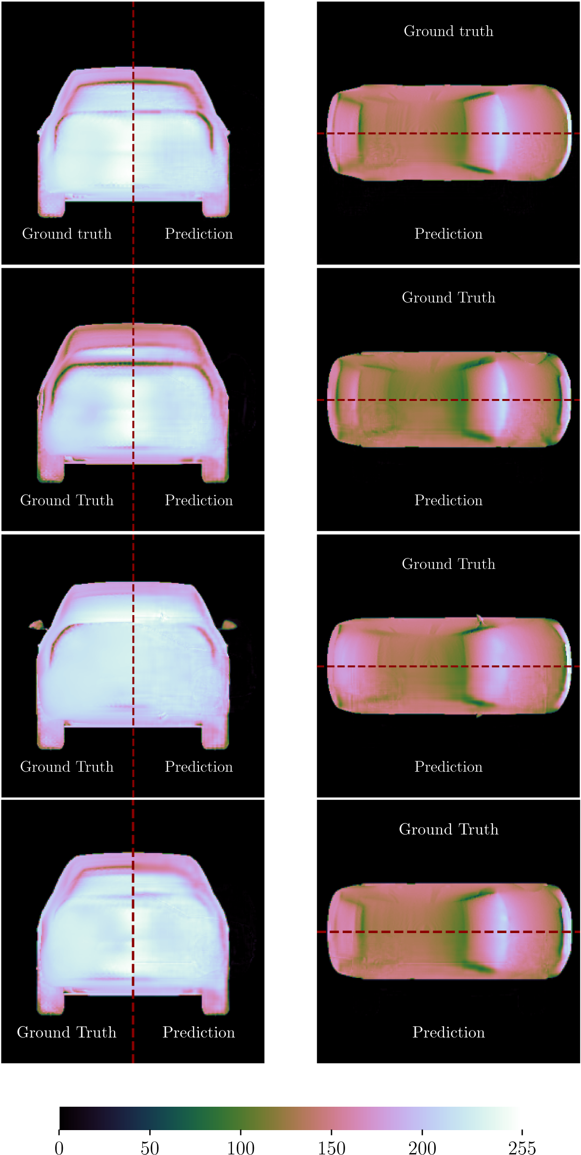
Figure 17. Long description
The grid consists of four rows, each representing a different vehicle model: DrivAer C H 3, DrivAer C H 4, DrivAer C H 5, and DrivAer C H 6.
Each row contains two panels. The left panel shows a rear view of the vehicle, and the right panel shows a top-down view. Every panel is bisected by a red dashed line. The area to the left or top of the dashed line is labeled Ground Truth, and the area to the right or bottom is labeled Prediction.
A color scale bar at the bottom ranges from 0 to 255. The scale transitions from black at 0, through dark teal at 50, olive green at 100, tan at 150, light pink at 200, and white at 255.
In the rear views, the pressure distribution is predominantly light pink and white across the trunk and rear bumper, with dark teal and green accents around the wheel wells and lower chassis. In the top-down views, the hood and roof show large areas of light pink, while the windshield and rear window areas exhibit dark green and teal bands indicating pressure changes. Across all four rows, the Prediction side closely mirrors the Ground Truth side in color intensity and spatial distribution, indicating high accuracy in the C sub p predictions.
4.2. A priori evaluation of DrivAerCH3
Beyond aggregate accuracy, the simplex structure of the datasets allows for a spatially resolved analysis of where predictions succeed or fail. One of the benefits of generating data within a simplex is that it allows for direct visualization of different samples in relation to each other. It also allows for the study of the accuracy in interpolation and extrapolation tasks in a controlled manner. Typically, extrapolation testing involves making inference on samples from out of the training set distribution, with the idea being that good predictive performance on these unseen samples suggests that the network is generalizing well. Using the ShapeCH procedure, we can make the process systematic, and introduce an a priori measure of extrapolation distance based on the inputs alone.
To do this, the following training–testing split of the DrivAerCH3 database is considered: the points inside the incircle of the barycentric triangle are used for training, and those outside are used for testing (see Figure 18). Using this split, the testing set and training set are not drawn from the same distribution; in fact, the two sets are completely disjoint on the map. However, it is vital to also note that the testing set is not completely disconnected from the training set: the two differ only by the ranges of the two free parameters used to generate the convex hull from the same basis cases. With this in mind, it becomes apparent that those samples in the testing set that lie closer to the circumference of the incircle are “closer” to the training set in the feature space, and are expected to be less challenging to predict, with the amount of extrapolation increasing with increasing distance away from the incircle. Thus, it is possible to assign an “extrapolation distance” to each sample in the testing set, simply computed as the Euclidean distance from the circumference. This is shown in Figure 19, expressed as a percentage ranging from 0% on the circle to 100% at the three vertices.
Extrapolation study: training set (top) and test set (bottom), shaded by
$ {C}_D $
 .
.
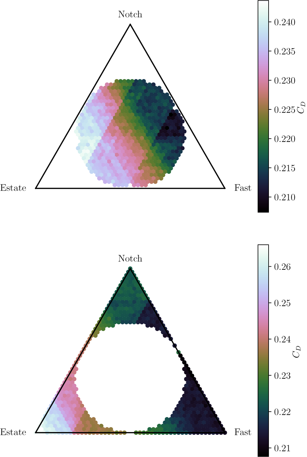
Figure 18. Long description
A multi-panel figure containing two ternary plots arranged vertically, each with a color scale bar on the right.
* Top Panel (Training Set): A triangle with vertices labeled Notch at the top, Fast at the bottom-right, and Estate at the bottom-left. A circular cluster of data points occupies the center of the triangle. The points are colored according to a C sub D scale ranging from 0.210 (black) to 0.240 (white). The data shows a gradient where lower values (dark green and black) are concentrated toward the Notch and Fast vertices, while higher values (light blue and white) are concentrated toward the Estate vertex.
* Bottom Panel (Test Set): The same ternary triangle structure. The data points are distributed along the perimeter of the triangle, leaving a large circular void in the center. The color scale for C sub D ranges from 0.21 to 0.26. High values (light blue) are located at the bottom-left corner near Estate. Low values (dark purple and black) are concentrated along the right edge toward the Fast vertex and the top corner near the Notch vertex.
Extrapolation distance (%).
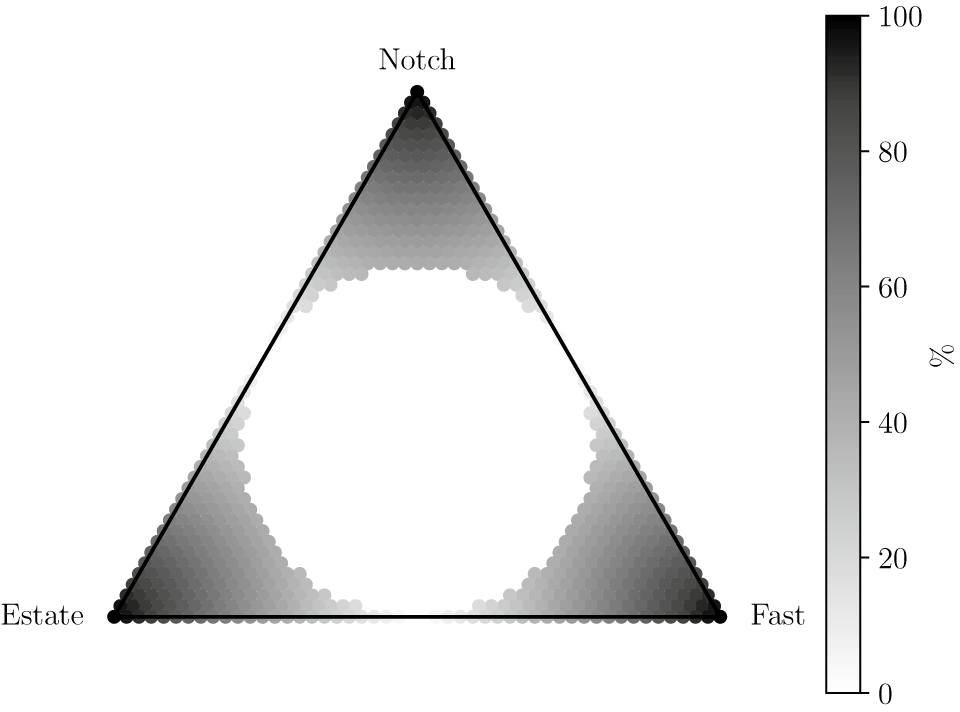
Figure 19. Long description
A ternary plot in the shape of an equilateral triangle with three labeled vertices. The top vertex is labeled Notch. The bottom-left vertex is labeled Estate. The bottom-right vertex is labeled Fast. The interior of the triangle contains a circular white void at the center, indicating 0 percent extrapolation distance. Moving from the center toward each of the three corners, the area is filled with small circular data points that transition from light gray to black. The highest density and darkest shading, representing 100 percent, are concentrated exactly at the three vertices. To the right of the triangle is a vertical color bar scale. The scale is labeled with a percent symbol and ranges from 0 at the bottom in white to 100 at the top in black, with intermediate markers at 20, 40, 60, and 80.
Next, a CNN to predict
$ {C}_D $
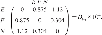
 (with similar specifications to the one before) is trained on the data inside the incircle. The expectation is that the network prediction error on the testing set will mirror the contours of Figure 19. The error is shown in Figure 20. It is seen that the lower left vertex, corresponding to the estateback basis case, has the spatial error distribution that is expected, with the error increasing radially outward from the incircle and reaching a maximum at the vertex. However, this behavior is not seen in the vicinity of the other two vertices. The key to resolving this anomalous behavior is to recognize that the extrapolation distance does not account for the actual basis cases assigned to each vertex of the simplex. In other words, Figure 20 is independent of the database. It is clear that a full picture of extrapolation distance must include the effect of varying basis cases, so that if a certain vertex (or basis case) is much further away than the others in feature space, this is reflected by a corresponding increase in the extrapolation distance toward that vertex. This may be alternatively thought of as a rescaling of the sides of the triangle to reflect distances between the basis configurations. To do this, we begin by computing the pairwise distance matrix (see Equation (1)) for the DrivAerCH3 database:
Test set relative error from extrapolation study.
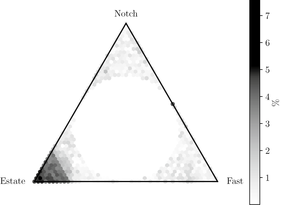
Figure 20. Long description
The ternary plot is an equilateral triangle with three labeled vertices. The top vertex is labeled Notch. The bottom-right vertex is labeled Fast. The bottom-left vertex is labeled Estate. The interior of the triangle is filled with a hexagonal heat map representing data density or error percentage.
* The highest concentration of dark hexagons, indicating higher relative error, is clustered heavily at the bottom-left corner near the Estate vertex.
* A secondary, much lighter concentration of hexagons is visible near the top Notch vertex.
* The area near the bottom-right Fast vertex and the center of the triangle are largely empty or contain very light, low-value hexagons.
* To the right of the triangle is a vertical color bar scale labeled with a percent symbol. The scale ranges from 1 at the bottom to 7 at the top. The gradient transitions from white at 1, through shades of gray, to solid black at 7.
The matrix has a zero leading diagonal by construction, and the off-diagonal elements represent pairwise distances between basis cases. Here, the letter
$ E $
 denotes the estateback,
$ F $
denotes the estateback,
$ F $
 the fastback, and
$ N $
the fastback, and
$ N $
 the notchback. It is observed that the distance between the notchback and the fastback (
$ 0.304\times {10}^{-4} $
the notchback. It is observed that the distance between the notchback and the fastback (
$ 0.304\times {10}^{-4} $
 ) is approximately a factor of three smaller than the distance between the estateback and the fastback, and a factor of four smaller than the distance between the notchback and the estateback. This information provides the coefficients required to rescale the extrapolation distances from Figure 19, in order to account for the relative differences between the basis cases in feature space. Upon rescaling the distances with the values from the earlier matrix, the modified distance map shown in Figure 21 is obtained. The map now paints a much more accurate picture of the extent to which the network is extrapolating, and it is clear that the higher accuracy of the predictions in the vicinity of the fastback and notchback vertices is due to the low feature space variation in those geometries, relative to the estateback vertex.
Test set relative error from extrapolation study rescaled by basis case diversity.
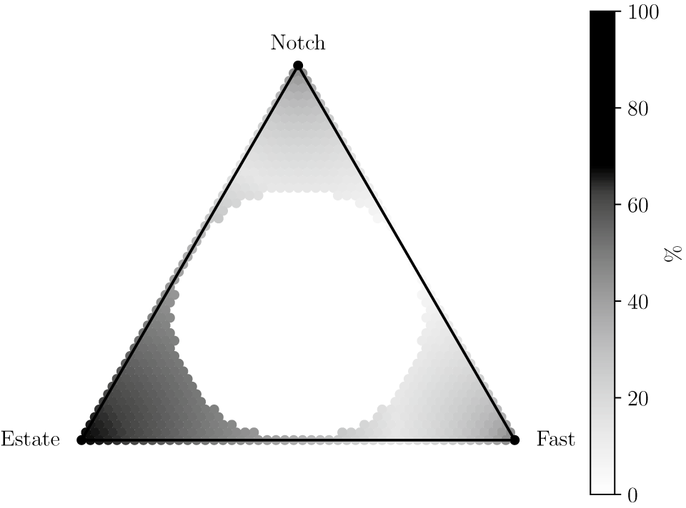
Figure 21. Long description
A triangular ternary plot with vertices labeled Notch at the top, Fast at the bottom right, and Estate at the bottom left. The interior of the triangle is filled with circular data points of varying grayscale shades. The highest error concentrations, indicated by darker shades, are clustered at the Estate vertex. The Notch and Fast vertices show lighter gray shades, indicating lower relative error. A large circular white void occupies the center of the triangle, where no data points are plotted. To the right of the triangle is a vertical color bar scale labeled with a percent symbol. The scale ranges from 0 at the bottom in white to 100 at the top in solid black, with numerical markers at 20, 40, 60, and 80.
4.3. A priori evaluation of DrivAerCH5
The earlier exercise is repeated for the higher diversity DrivAerCH5 dataset, which has two SUV configurations in addition to the three sedans (see Table 6). The MDS projection in 2D is again used to divide the 715 samples into 357 training and 358 test set samples (see Figure 21). This is unlike the division of the barycentric triangle for the previous section in that it is sensitive to the numerical computation of the MDS (Figure 22). The training is done using the CNN architecture from Section 3.5. The results of the training are shown in Figure 23. The error plot shows a concentration of poor predictions in the subsimplex with the vertices corresponding to the SUV models. As before, we compute the rescaled extrapolation distances using the SDFs of the five basis geometries, and plot them on the MDS projection. It is seen that the regions of high extrapolation distance correlate well with the inference error plot again. One notes that the prediction error is in fact lower than that expected from the extrapolation distances. The reason is because the diversity metric is conditioned on the input (geometric) space to allow for a priori assessments of the test samples. In this case, the results indicate a more expressive geometric space than the corresponding output drag space, so that the model performs better than expected in regions with predominantly the sedan configurations.
Controlled extrapolation test of
$ {C}_D $
 prediction on the DrivAerCH5 dataset; left: MDS projection of training set, colored by
$ {C}_D $
prediction on the DrivAerCH5 dataset; left: MDS projection of training set, colored by
$ {C}_D $
 value; right: testing set.
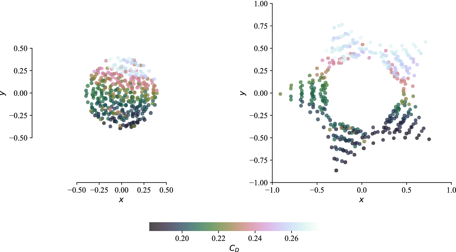
Figure 22. Long description
A two-panel scatter plot visualization using M D S projections.
Left Panel: Training set. The x and y axes both range from negative 0.50 to 0.50. The data points form a dense, solid circular cluster centered at the origin. The colors transition vertically from dark grey and navy at the bottom (y equals negative 0.50), through green and pink in the middle, to light blue at the top (y equals 0.50).
Right Panel: Testing set. The x and y axes range from negative 1.0 to 1.0. The data points are arranged in a ring-like structure with a hollow center around the origin. The points extend further outward than the training set, forming a star-like or hexagonal perimeter. The color gradient follows the same vertical pattern as the left panel, with dark shades at the bottom and light blue at the top.
Bottom: A horizontal color scale bar labeled C sub D. It ranges from 0.20 to 0.26. The gradient moves from dark grey (0.20) to teal (0.22), then to light pink (0.24), and finally to pale blue (0.26).
Controlled extrapolation test of
$ {C}_D $
 prediction on the DrivAerCH5 dataset. MDS projections of: (a)
$ {C}_D $
prediction on the DrivAerCH5 dataset. MDS projections of: (a)
$ {C}_D $
 network predictions, (b)
$ {C}_D $
network predictions, (b)
$ {C}_D $
 ground truth values, (c) relative error, (d) extrapolation distances computed from diversity metric.
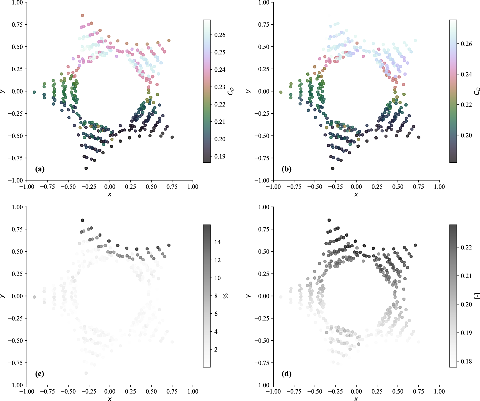
Figure 23. Long description
The four scatter plots are arranged in a two by two grid. All plots share identical x and y axes representing M D S coordinates from negative 1.00 to 1.00. The data points form a distinct hexagonal ring shape with a hollow center.
Panel a, top-left, shows C sub D network predictions. Points are colored by a gradient from dark blue at the bottom to light pink at the top. A color bar to the right indicates C sub D values from 0.19 to 0.26.
Panel b, top-right, shows C sub D ground truth values. The color distribution is nearly identical to panel a, indicating high prediction accuracy across the hexagonal manifold.
Panel c, bottom-left, shows relative error as a percentage. The color bar ranges from 2 to 14 percent. Most points are very light gray, indicating low error, with slightly darker gray points concentrated at the top and bottom vertices of the hexagon.
Panel d, bottom-right, shows extrapolation distances computed from a diversity metric. The color bar ranges from 0.18 to 0.22. The points show a gradient where the left side of the hexagon is lighter and the right side is darker gray, indicating increasing extrapolation distance along the positive x axis.
The preceding analysis shows that the simplex geometry, combined with the diversity metric, enables a priori identification of regions where prediction is difficult. A natural follow-up is to ask whether a global relationship between dataset characteristics and prediction error exists.
4.4. Scaling experiments
The qualitative observation that accuracy degrades with diversity motivates a quantitative investigation. In this section, a series of controlled experiments is designed to isolate the effects of dataset size
$ m $
 and diversity
$ M $
and diversity
$ M $
 on the prediction error. The goal is to determine whether a scaling law exists that collapses the error from all experiments onto a single curve parameterized by
$ M $
on the prediction error. The goal is to determine whether a scaling law exists that collapses the error from all experiments onto a single curve parameterized by
$ M $
 and
$ m $
and
$ m $
 alone.
Recall from Table 6 that
$ M $
 ,
$ g $
,
$ g $
 ,
$ m $
,
$ m $
 , and the simplex dimension
$ p $
, and the simplex dimension
$ p $
 are not independent: for a uniformly sampled
$ p $
are not independent: for a uniformly sampled
$ p $
 -simplex with
$ g $
-simplex with
$ g $
 points per edge,
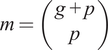
$ m=\left(\begin{array}{c}g+p\\ {}p\end{array}\right) $
points per edge,
$ m=\left(\begin{array}{c}g+p\\ {}p\end{array}\right) $
 . Furthermore, the normalization of the diversity metric (Equation (2)) couples
$ M $
. Furthermore, the normalization of the diversity metric (Equation (2)) couples
$ M $
 to
$ p $
to
$ p $
 through the number of basis-case pairs. Consequently, it is not possible to vary each of
$ M $
through the number of basis-case pairs. Consequently, it is not possible to vary each of
$ M $
 ,
$ g $
,
$ g $
 ,
$ m $
,
$ m $
 , and
$ p $
, and
$ p $
 independently. Rather than attempting to disentangle these coupled quantities, the approach adopted here is empirical: six families of experiments are designed, each targeting a different combination of the design variables, and a scaling law is sought that collapses all of them simultaneously.
The experiment families are designed to isolate these effects by holding one quantity constant at a time. Constant-size experiments fix
$ m $
 and vary the simplex (and thus
$ M $
and vary the simplex (and thus
$ M $
 ), revealing the effect of diversity alone. Constant-diversity experiments fix the simplex (and thus
$ M $
), revealing the effect of diversity alone. Constant-diversity experiments fix the simplex (and thus
$ M $
 ) and extract barycentric subgrids at different grid densities
$ g $
) and extract barycentric subgrids at different grid densities
$ g $
 , varying size through the combinatorial constraint. Constant-density experiments fix the grid density (
$ g=3 $
, varying size through the combinatorial constraint. Constant-density experiments fix the grid density (
$ g=3 $
 and
$ g=5 $
and
$ g=5 $
 ) across DrivAerCH4–CH6, so that
$ m $
) across DrivAerCH4–CH6, so that
$ m $
 and
$ M $
and
$ M $
 both grow with the simplex dimension. All three types are summarized in Table 7.
Summary of scaling experiments
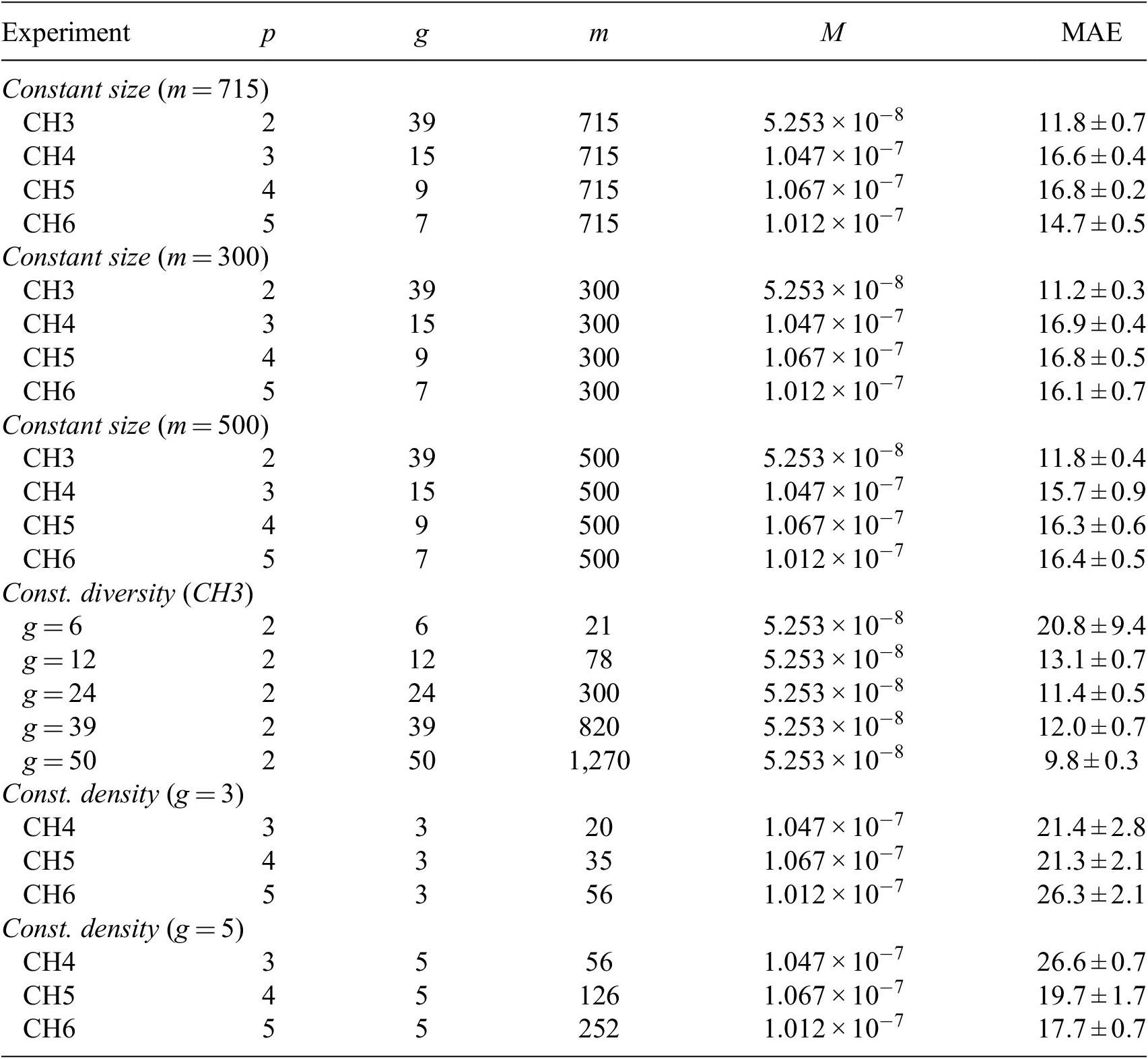
Table 7. Long description
The table is organized into six columns: Experiment, p (simplex dimension), g (grid density), m (training samples), M (diversity metric), and M A E (Mean Absolute Error).
* Constant size (m = 715):
- C H 3: p=2, g=39, m=715, M=5.253 times 10 super -8, M A E=11.8 plus or minus 0.7.
- C H 4: p=3, g=15, m=715, M=1.047 times 10 super -7, M A E=16.6 plus or minus 0.4.
- C H 5: p=4, g=9, m=715, M=1.067 times 10 super -7, M A E=16.8 plus or minus 0.2.
- C H 6: p=5, g=7, m=715, M=1.012 times 10 super -7, M A E=14.7 plus or minus 0.5.
* Constant size (m = 300):
- C H 3: p=2, g=39, m=300, M=5.253 times 10 super -8, M A E=11.2 plus or minus 0.3.
- C H 4: p=3, g=15, m=300, M=1.047 times 10 super -7, M A E=16.9 plus or minus 0.4.
- C H 5: p=4, g=9, m=300, M=1.067 times 10 super -7, M A E=16.8 plus or minus 0.5.
- C H 6: p=5, g=7, m=300, M=1.012 times 10 super -7, M A E=16.1 plus or minus 0.7.
* Constant size (m = 500):
- C H 3: p=2, g=39, m=500, M=5.253 times 10 super -8, M A E=11.8 plus or minus 0.4.
- C H 4: p=3, g=15, m=500, M=1.047 times 10 super -7, M A E=15.7 plus or minus 0.9.
- C H 5: p=4, g=9, m=500, M=1.067 times 10 super -7, M A E=16.3 plus or minus 0.6.
- C H 6: p=5, g=7, m=500, M=1.012 times 10 super -7, M A E=16.4 plus or minus 0.5.
* Constant diversity (C H 3):
- g=6: p=2, g=6, m=21, M=5.253 times 10 super -8, M A E=20.8 plus or minus 9.4.
- g=12: p=2, g=12, m=78, M=5.253 times 10 super -8, M A E=13.1 plus or minus 0.7.
- g=24: p=2, g=24, m=300, M=5.253 times 10 super -8, M A E=11.4 plus or minus 0.5.
- g=39: p=2, g=39, m=820, M=5.253 times 10 super -8, M A E=12.0 plus or minus 0.7.
- g=50: p=2, g=50, m=1,270, M=5.253 times 10 super -8, M A E=9.8 plus or minus 0.3.
* Constant density (g = 3):
- C H 4: p=3, g=3, m=20, M=1.047 times 10 super -7, M A E=21.4 plus or minus 2.8.
- C H 5: p=4, g=3, m=35, M=1.067 times 10 super -7, M A E=21.3 plus or minus 2.1.
- C H 6: p=5, g=3, m=56, M=1.012 times 10 super -7, M A E=26.3 plus or minus 2.1.
* Constant density (g = 5):
- C H 4: p=3, g=5, m=56, M=1.047 times 10 super -7, M A E=26.6 plus or minus 0.7.
- C H 5: p=4, g=5, m=126, M=1.067 times 10 super -7, M A E=19.7 plus or minus 1.7.
- C H 6: p=5, g=5, m=252, M=1.012 times 10 super -7, M A E=17.7 plus or minus 0.7.
Note. Here
$ p $
 is the simplex dimension,
$ g $
is the simplex dimension,
$ g $
 the grid density (points per edge),
$ m $
the grid density (points per edge),
$ m $
 the number of training samples,
$ M $
the number of training samples,
$ M $
 the diversity metric, and MAE the mean absolute error in drag counts (one drag count
$ =\Delta {C}_D=0.001 $
the diversity metric, and MAE the mean absolute error in drag counts (one drag count
$ =\Delta {C}_D=0.001 $
 ) for the best-performing hyperparameter configuration. The
$ \pm $
) for the best-performing hyperparameter configuration. The
$ \pm $
 range denotes the 95% confidence interval over eight hyperparameter configurations (see text), quantifying network sensitivity.
All 23 experiments use the CNN architecture described in Section 2.4. To ensure that the scaling behavior is not an artifact of a single network configuration, each experiment is repeated with eight hyperparameter settings drawn from a
$ 2\times 2\times 2 $
 grid: number of convolutional layers
$ \in \left\{3,4\right\} $
grid: number of convolutional layers
$ \in \left\{3,4\right\} $
 , channel width
$ \in \left\{\mathrm{64,128}\right\} $
, channel width
$ \in \left\{\mathrm{64,128}\right\} $
 , and batch size
$ \in \left\{16,32\right\} $
, and batch size
$ \in \left\{16,32\right\} $
 , yielding networks with approximately 218,000 to 690,000 trainable parameters. The learning rate (
$ {10}^{-4} $
, yielding networks with approximately 218,000 to 690,000 trainable parameters. The learning rate (
$ {10}^{-4} $
 ) and number of epochs (500) are held fixed. For each of the
$ 23\times 8=184 $
) and number of epochs (500) are held fixed. For each of the
$ 23\times 8=184 $
 configurations, fivefold cross-validation is performed, so that a total of 920 networks are trained from scratch. The reported MAE for each experiment is the fivefold mean of the best-performing hyperparameter configuration, and the
$ \pm $
configurations, fivefold cross-validation is performed, so that a total of 920 networks are trained from scratch. The reported MAE for each experiment is the fivefold mean of the best-performing hyperparameter configuration, and the
$ \pm $
 bounds in Table 7 are 95% confidence intervals computed from the eight configuration means using a
$ t $
bounds in Table 7 are 95% confidence intervals computed from the eight configuration means using a
$ t $
 distribution with seven degrees of freedom. These intervals isolate the sensitivity of the prediction error to the network architecture. In all cases, the MAE is evaluated on the held-out test fold, so that every sample is predicted exactly once by a network that never saw it during training.
4.5. Scaling law
To quantify the impact of dataset size, density, and diversity, a relationship between the prediction error and the dataset characteristics is sought. The most general form, involving all four characterization variables, is

where
$ \varepsilon $
 denotes the MAE,
$ {\varepsilon}_0 $
denotes the MAE,
$ {\varepsilon}_0 $
 absorbs the irreducible loss and order-unity coefficients, and
$ a $
absorbs the irreducible loss and order-unity coefficients, and
$ a $
 ,
$ b $
,
$ b $
 ,
$ c $
,
$ c $
 ,
$ d $
,
$ d $
 are exponents to be determined. Taking logarithms converts (4) to a linear regression, and ordinary least squares is applied to the 23 data points from Table 7.
The full four-variable fit yields
$ {R}^2=0.88 $
 , but the exponents on
$ g $
, but the exponents on
$ g $
 and
$ p $
and
$ p $
 are not statistically significant (
$ {p}_g=0.35 $
are not statistically significant (
$ {p}_g=0.35 $
 ,
$ {p}_p=0.54 $
,
$ {p}_p=0.54 $
 ); their information is already captured by
$ M $
); their information is already captured by
$ M $
 and
$ m $
and
$ m $
 through the combinatorial constraint
$ m=\left(\begin{array}{c}g+p\\ {}p\end{array}\right) $
through the combinatorial constraint
$ m=\left(\begin{array}{c}g+p\\ {}p\end{array}\right) $
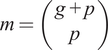 , which makes
$ m $
, which makes
$ m $
 ,
$ g $
,
$ g $
 , and
$ p $
, and
$ p $
 collinear. Conversely, fitting
$ m $
collinear. Conversely, fitting
$ m $
 ,
$ g $
,
$ g $
 , and
$ p $
, and
$ p $
 without
$ M $
without
$ M $
 yields
$ {R}^2=0.82 $
yields
$ {R}^2=0.82 $
 with no individually significant exponent (
$ {p}_m=0.80 $
with no individually significant exponent (
$ {p}_m=0.80 $
 ,
$ {p}_g=0.09 $
,
$ {p}_g=0.09 $
 ,
$ {p}_p=0.84 $
,
$ {p}_p=0.84 $
 ), confirming that
$ M $
), confirming that
$ M $
 carries information that the other variables cannot replace. Including only
$ M $
carries information that the other variables cannot replace. Including only
$ M $
 and
$ m $
and
$ m $
 gives
gives

with negligible loss in explanatory power and both exponents highly significant (
$ p<{10}^{-3} $
 ). The grid density
$ g $
). The grid density
$ g $
 and simplex dimension
$ p $
and simplex dimension
$ p $
 are therefore dropped, yielding the scaling law:
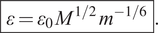
The quality of the scaling law is shown in Figure 24. A composite scaling variable
$ \xi \propto {M}^{1/2}\hskip0.1em {m}^{-1/6} $
 is formed, and the MAE of all 23 experiments is plotted against
$ \xi $
is formed, and the MAE of all 23 experiments is plotted against
$ \xi $
 . Error bars indicate the standard error of the mean across the five cross-validation folds, which is largest for the low-
$ m $
. Error bars indicate the standard error of the mean across the five cross-validation folds, which is largest for the low-
$ m $
 experiments (up to
$ \pm 10 $
experiments (up to
$ \pm 10 $
 drag counts for
$ m=20 $
drag counts for
$ m=20 $
 ) and negligible for well-sampled datasets. The narrow confidence intervals reported in Table 7 confirm that the collapse is not an artifact of a specific network architecture. The data from all experiment families (spanning different simplex dimensions, densities, sizes, and diversities) fall on a single line, confirming that the prediction error is governed by two quantities alone: the diversity of the basis shapes and the number of training samples.
All 23 experiments from Table 7 plotted against the composite variable
$ \xi \propto {M}^{1/2}\hskip0.1em {m}^{-1/6} $
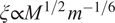 (scaled by
$ {10}^5 $
(scaled by
$ {10}^5 $
 for readability). Colors distinguish the six experiment families; markers denote the constraint type (circles: constant size; squares: constant density; triangles: constant diversity). Error bars show the standard error of the mean MAE across the five cross-validation folds of the best-performing network. The dashed line is the fit from Equation (6).
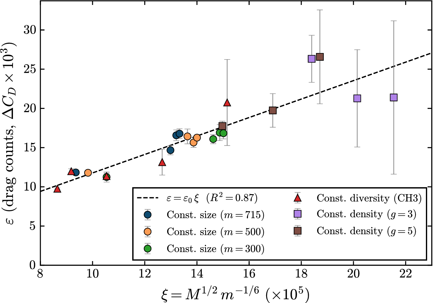
Figure 24. Long description
A line graph with a horizontal x-axis labeled xi equals M super 1/2 m super minus 1/6 times 10 super 5, ranging from 8 to 22. The vertical y-axis is labeled epsilon (drag counts, delta C sub D times 10 super 3), ranging from 0 to 30.
* Data Points: Twenty-three markers are plotted, showing a positive linear trend.
* Trend Line: A dashed black line represents the fit epsilon equals epsilon sub 0 xi with an R-squared value of 0.87, originating near y equals 10 at x equals 8 and rising to y equals 27 at x equals 23.
* Legend: Located at the bottom right, it identifies six categories:
- Blue circles: Const. size (m equals 715)
- Orange circles: Const. size (m equals 500)
- Green circles: Const. size (m equals 300)
- Red triangles: Const. diversity (C H 3)
- Purple squares: Const. density (g equals 3)
- Brown squares: Const. density (g equals 5)
* Error Bars: Vertical grey bars indicate standard error, which increases in magnitude as xi increases, particularly for the purple and brown square markers at the higher end of the x-axis.
The dependence on dataset size (
$ {m}^{-1/6} $
 ) is considerably weaker than the dependence on diversity (
$ {M}^{1/2} $
) is considerably weaker than the dependence on diversity (
$ {M}^{1/2} $
 ): a tenfold increase in training samples reduces the MAE by roughly 33%, whereas the same factor in diversity increases it by more than threefold. This asymmetry suggests that, beyond a certain dataset size, further gains are better achieved by controlling the diversity of the basis shapes than by adding more samples.
The exponent
$ b=-1/6 $
 on dataset size is notably weaker than the
$ {m}^{-1/2} $
on dataset size is notably weaker than the
$ {m}^{-1/2} $
 convergence rate of Monte Carlo estimators based on independent samples. This is expected: the training geometries are not independent but are generated by barycentric interpolation of a small number of basis shapes, introducing strong correlations among samples. This sub-MC convergence is a manifestation of oversampling in synthetic datasets and suggests that the scaling law (6) may not generalize to parametrizations with weaker intersample correlations, where a steeper exponent could be expected. Neither the grid density
$ g $
convergence rate of Monte Carlo estimators based on independent samples. This is expected: the training geometries are not independent but are generated by barycentric interpolation of a small number of basis shapes, introducing strong correlations among samples. This sub-MC convergence is a manifestation of oversampling in synthetic datasets and suggests that the scaling law (6) may not generalize to parametrizations with weaker intersample correlations, where a steeper exponent could be expected. Neither the grid density
$ g $
 nor the simplex dimension
$ p $
nor the simplex dimension
$ p $
 appear explicitly in (6). This is not because they are irrelevant, but because their effects are fully absorbed by
$ M $
appear explicitly in (6). This is not because they are irrelevant, but because their effects are fully absorbed by
$ M $
 and
$ m $
and
$ m $
 . The diversity metric
$ M $
. The diversity metric
$ M $
 already encodes
$ p $
already encodes
$ p $
 through its normalization over
$ p\left(p+1\right) $
through its normalization over
$ p\left(p+1\right) $
 basis-case pairs, and the sample count
$ m $
basis-case pairs, and the sample count
$ m $
 absorbs both
$ g $
absorbs both
$ g $
 and
$ p $
and
$ p $
 through the combinatorial constraint
$ m=\left(\begin{array}{c}g+p\\ {}p\end{array}\right) $
through the combinatorial constraint
$ m=\left(\begin{array}{c}g+p\\ {}p\end{array}\right) $
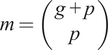 . As shown earlier, including
$ g $
. As shown earlier, including
$ g $
 and
$ p $
and
$ p $
 as additional regressors, improves
$ {R}^2 $
as additional regressors, improves
$ {R}^2 $
 by less than 0.01, confirming that these variables carry no independent information beyond what is already captured by
$ M $
by less than 0.01, confirming that these variables carry no independent information beyond what is already captured by
$ M $
 and
$ m $
and
$ m $
 .
.
Unlike neural scaling laws for large models (Kaplan et al., Reference Kaplan, McCandlish, Henighan, Brown, Chess, Child, Gray, Radford, Wu and Amodei2020), which include the number of model parameters
$ N $
 as an explicit variable, Equation (6) omits
$ N $
as an explicit variable, Equation (6) omits
$ N $
 . Each of the 23 experiments in Table 7 is repeated with eight network configurations spanning a threefold range in parameter count (218,000–690,000), and the resulting variation in MAE is small compared with the interexperiment differences: the median 95% confidence interval from the eight configurations is 0.7 drag counts, while the dataset-driven MAE ranges from 9.8 to 26.6 drag counts. At the relatively modest network and dataset sizes considered here, network capacity is therefore a secondary effect, and the prediction error is dominated by the dataset characteristics
$ M $
. Each of the 23 experiments in Table 7 is repeated with eight network configurations spanning a threefold range in parameter count (218,000–690,000), and the resulting variation in MAE is small compared with the interexperiment differences: the median 95% confidence interval from the eight configurations is 0.7 drag counts, while the dataset-driven MAE ranges from 9.8 to 26.6 drag counts. At the relatively modest network and dataset sizes considered here, network capacity is therefore a secondary effect, and the prediction error is dominated by the dataset characteristics
$ M $
 and
$ m $
and
$ m $
 .
.
The implication of the earlier for practitioners is clear: when designing a dataset for solving shape-to-performance studies, the two decisions that matter are (i) how geometrically diverse the basis shapes should be and (ii) how many samples to generate. The choice of simplex dimension or grid density is secondary, as long as the resulting
$ m $
 is sufficient. An explicit measure of shape diversity (not necessarily what is suggested here) is the most critical tool to evaluate existing datasets or generating new ones.
5. Conclusions
In this study, a conceptual framework for characterizing datasets used for building machine learning models is introduced. The application revolves around a shape-to-aerodynamic prediction task relevant to automotive design, though it is general in nature. Specifically, we consider size, density, and diversity as key metrics for characterizing the dataset. Size and density refer to the total number of samples and the coverage of the shape parametrization, respectively. Diversity is, instead, a quantitative metric describing the overall variety in the dataset.
The diversity measure relies on the signed distance function and the choice of few basis geometries. Only the input geometrical shapes are considered to demonstrate that the diversity in the input space is correlated with the diversity in the output space (Figure 11). This enables to estimate the “learning complexity” a priori in the absence of ground truth data (i.e., before extensive resources are devoted to generate simulation data).
Four different datasets are generated using a different number of basis configurations (from 3 to 6); the datasets are designed to have fixed size but varying density and diversity. When data-driven models are trained on these datasets, it is observed that there is an inverse correlation between model accuracy and dataset diversity. This observation is made precise by an empirical scaling law,
$ \varepsilon ={\varepsilon}_0\hskip0.1em {M}^{1/2}\hskip0.1em {m}^{-1/6} $
 , which collapses 23 controlled experiments spanning different simplex dimensions, grid densities, and dataset sizes onto a single curve (
$ {R}^2=0.87 $
, which collapses 23 controlled experiments spanning different simplex dimensions, grid densities, and dataset sizes onto a single curve (
$ {R}^2=0.87 $
 ). The scaling reveals that diversity has a substantially stronger effect on prediction error than dataset size, offering a practical guideline for dataset design. The proposed framework and characterization allows for meaningful comparisons between different databases.
Finally, geometries generated using the proposed approach lend themselves to a natural low-dimensional encoding given by the convex interpolation weights (or, equivalently, coordinates within the simplex). This allows for the definition of an extrapolation distance that quantifies how close new samples are to the existing training set. This is demonstrated in a controlled manner by a novel training–testing split, and examining the correlation between extrapolation distance and model inference accuracy. It is seen that the correlation is uncovered when the diversity of the basis cases is properly accounted for.
Taken together, these results underscore that data for learning must precede learning from data: before investing in model architecture or training, one must ensure that the dataset itself is adequate. The characterization framework introduced here provides the tools to make that assessment rigorously.
Data availability statement
The DrivAerCH3 dataset is available at the following repository: https://huggingface.co/datasets/mulligatawnysoup/DrivAerCH3 (Benjamin and Iaccarino, Reference Benjamin and Iaccarino2025a). The DrivAerCH4, DrivAerCH5, and DrivAerCH6 datasets are available at https://huggingface.co/datasets/mulligatawnysoup/DrivAerCHX (Benjamin and Iaccarino, Reference Benjamin and Iaccarino2025b). The ShapeCH repository can be found at https://code.stanford.edu/markben/ShapeCH. Other scripts used for the experiments in this work may be obtained by communicating with the authors directly.
Acknowledgments
The authors acknowledge useful discussions with Dr Frank Ham and Kun Lu at Cadence Design Systems, San Jose, CA. The computations performed in this study were performed on the NREL Kestrel HPC Cluster in Golden, CO. The authors acknowledge the use of LLM-based coding assistants during the conduct of this work.
Author contribution
Data curation: M.B., G.I.; Formal analysis: M.B.; Investigation: M.B., G.I.; Methodology: M.B., G.I.; Project administration: M.B., G.I.; Resources: M.B., G.I.; Software: M.B.; Supervision: M.B., G.I.; Writing - original draft: M.B.; Conceptualization: G.I.; Funding acquisition: G.I.; Validation: G.I.; Writing - review & editing: G.I.
Funding statement
This work was funded by the Franklin & Caroline Johnson Fellowship at the Stanford University.
Competing interests
The authors are aware of no competing interests that could potentially have impacted the conclusions drawn from this work.
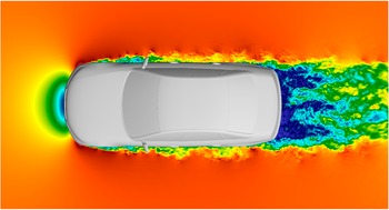
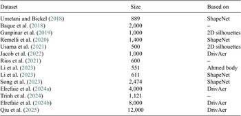
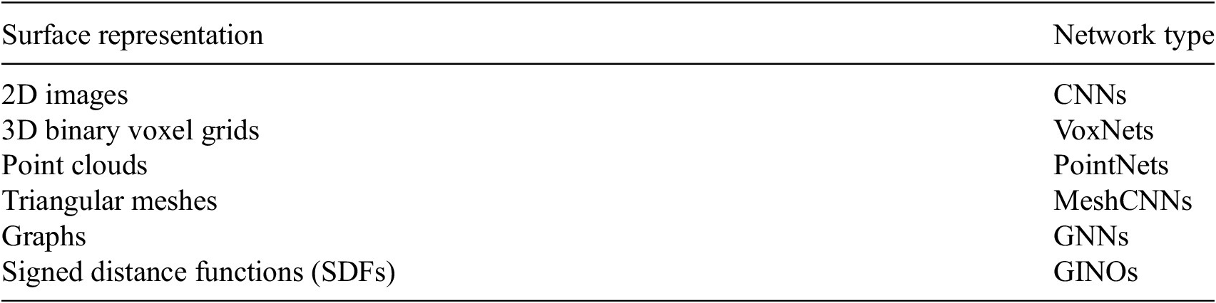
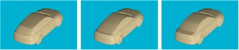
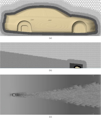
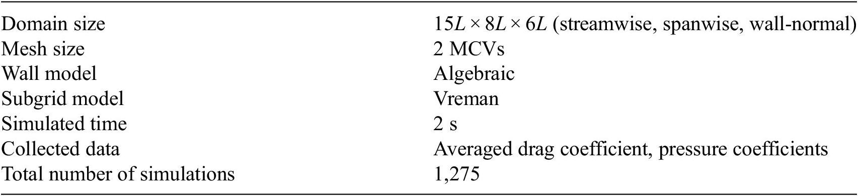
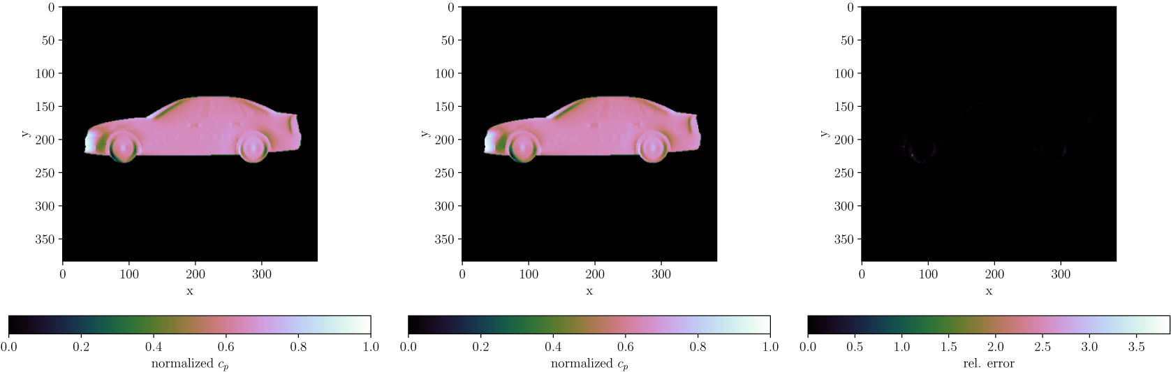
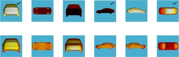
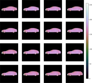

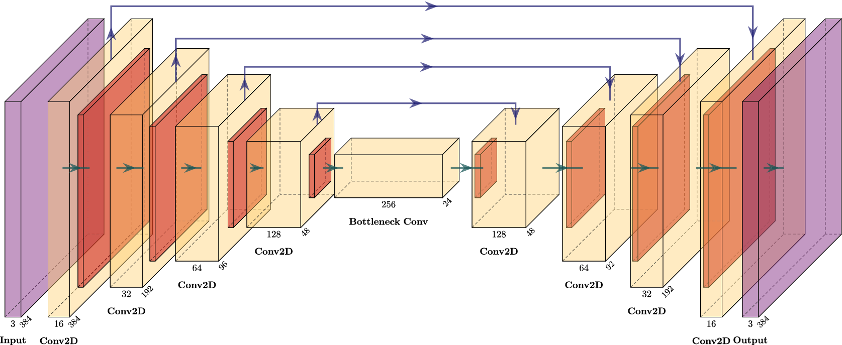

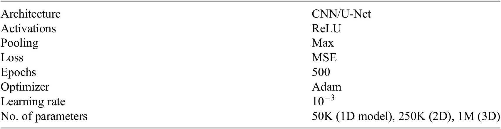
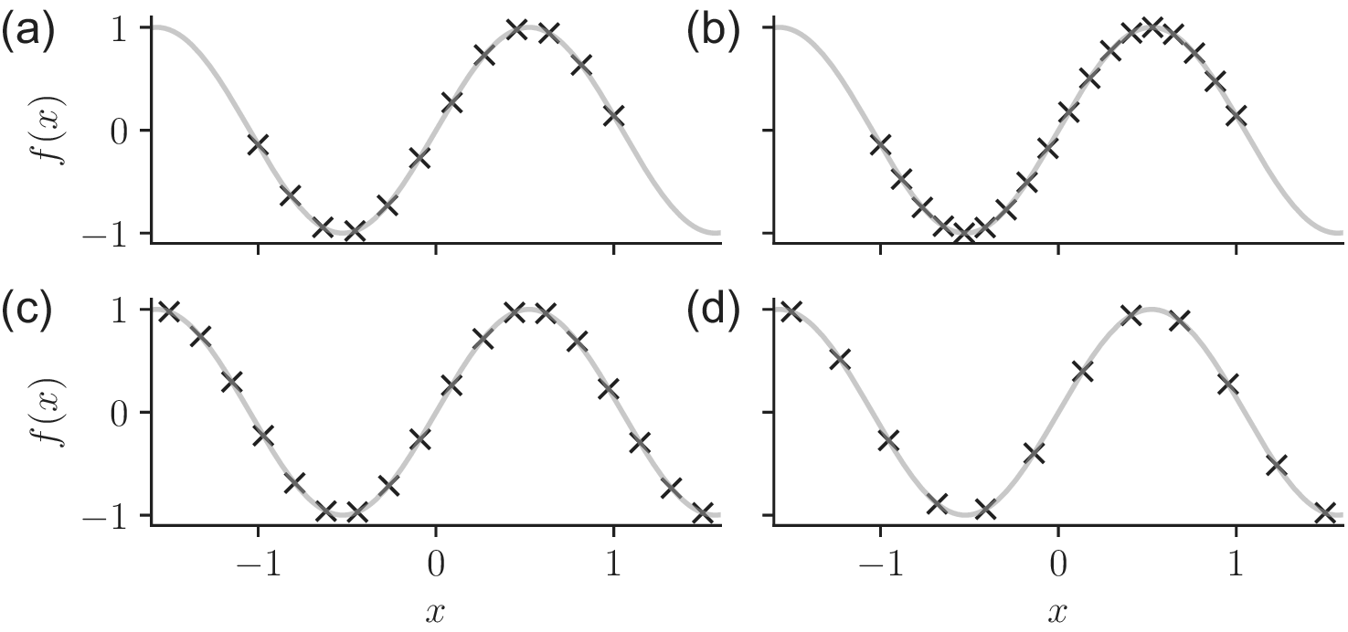

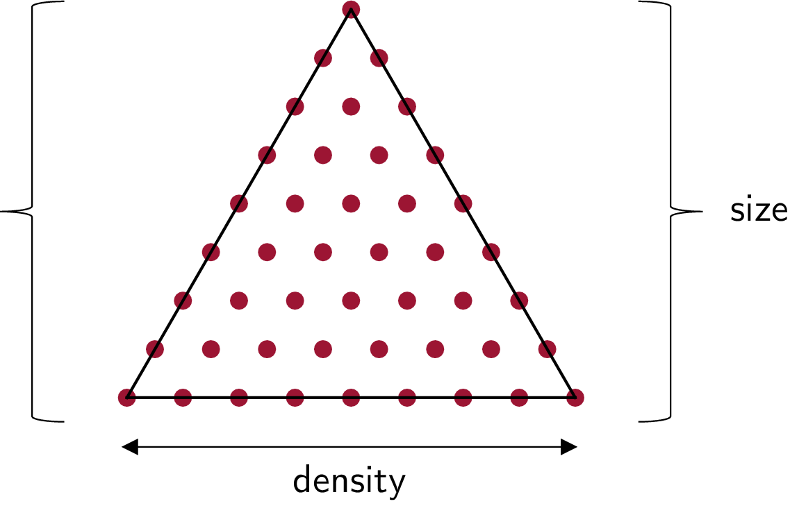
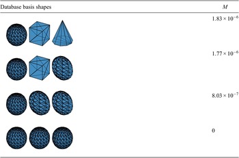
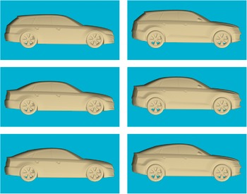
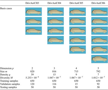
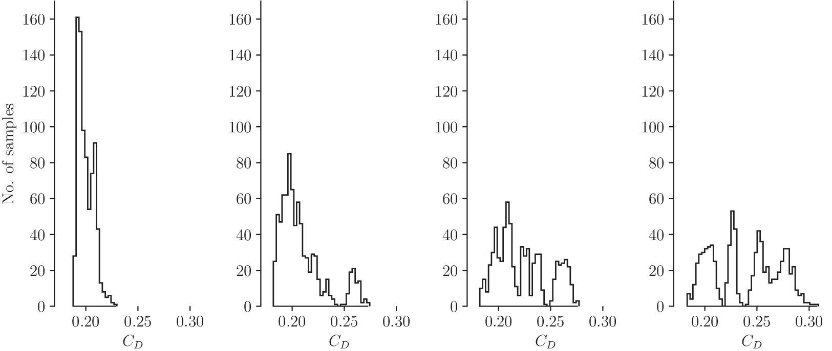
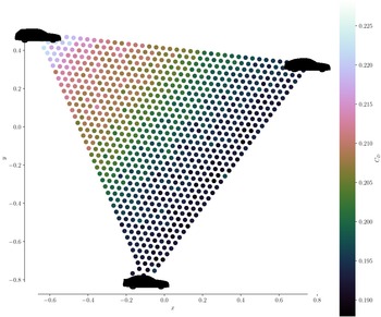
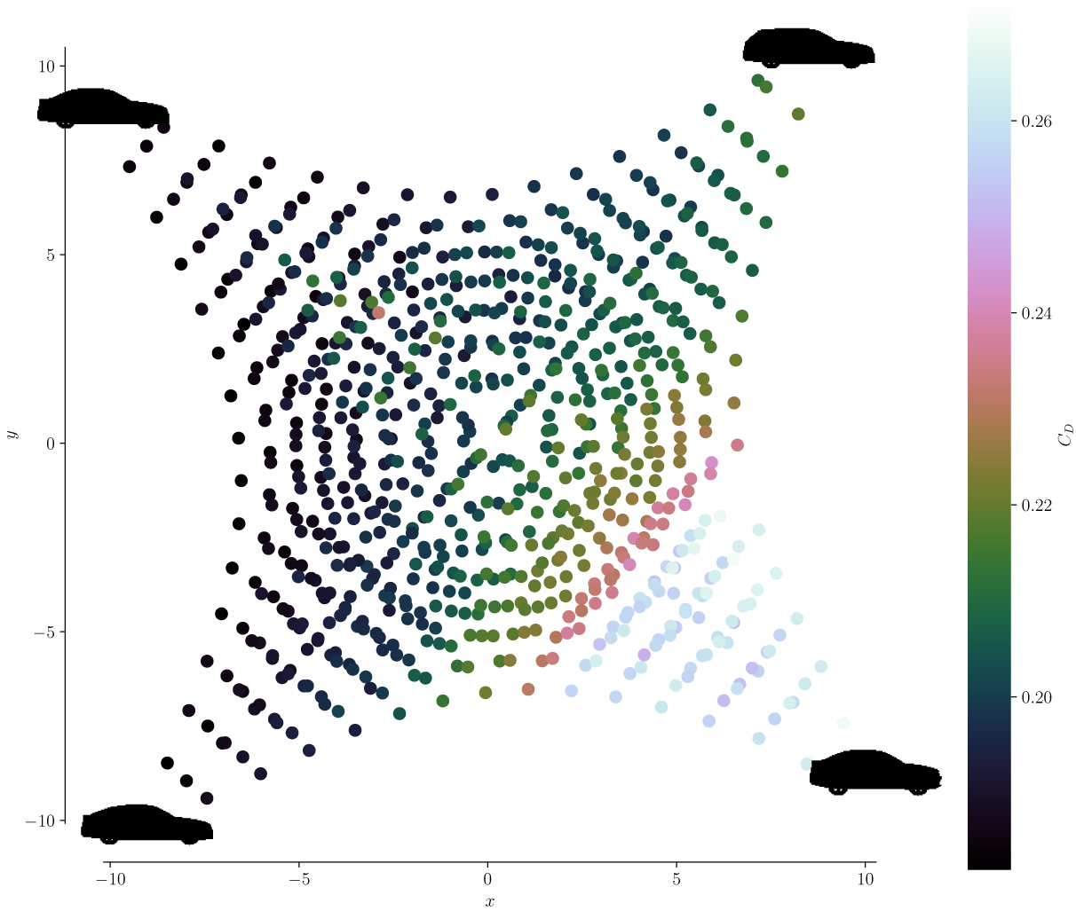
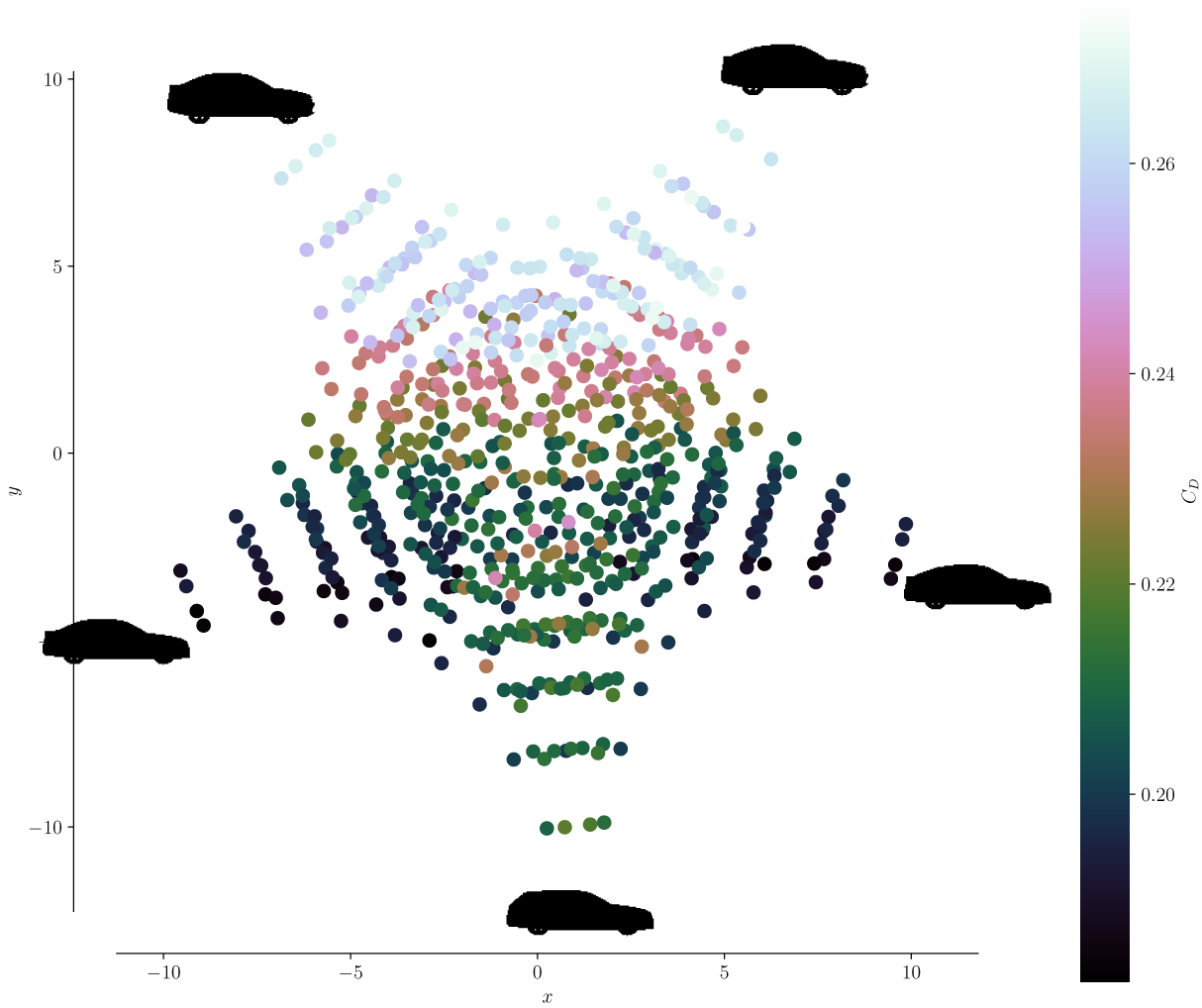
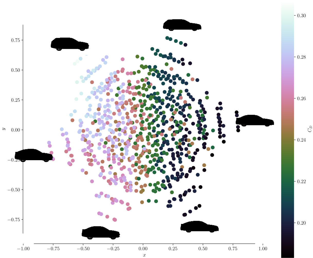
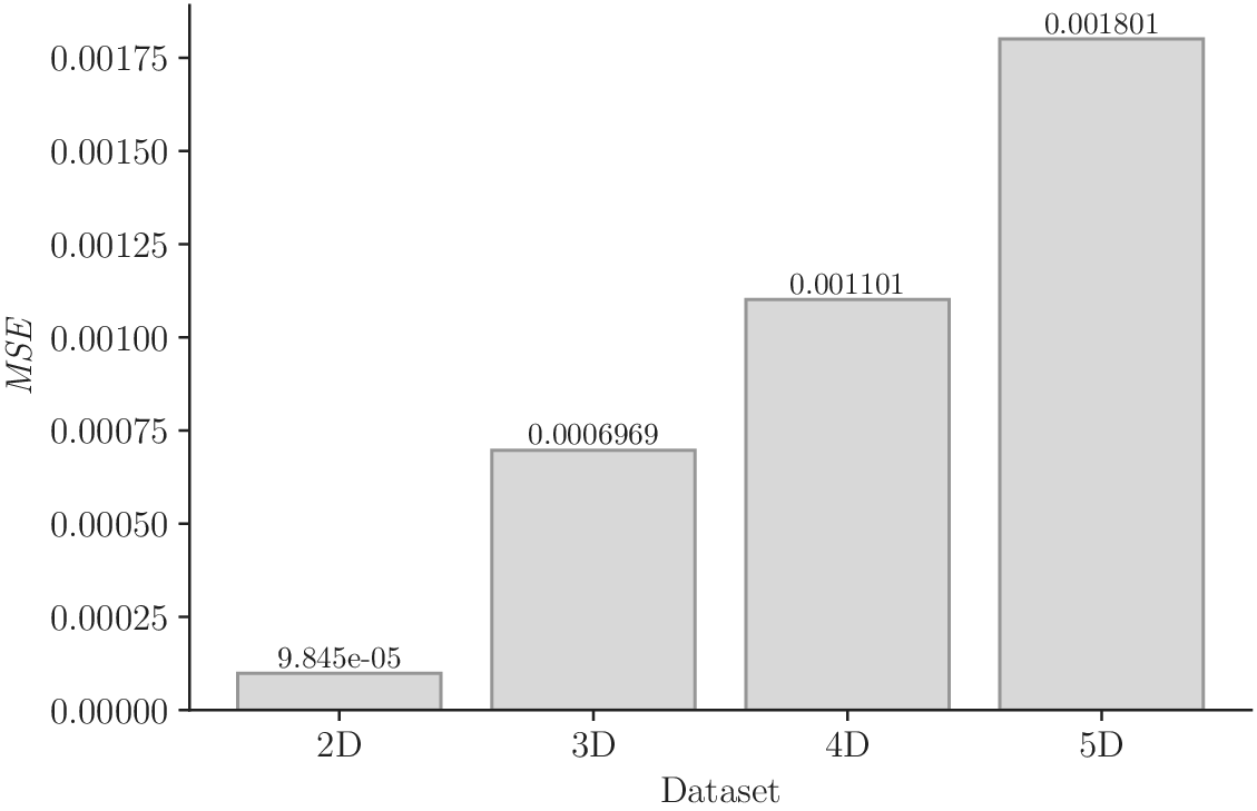
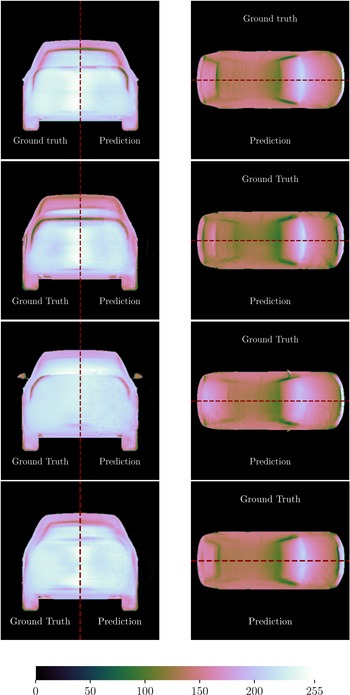

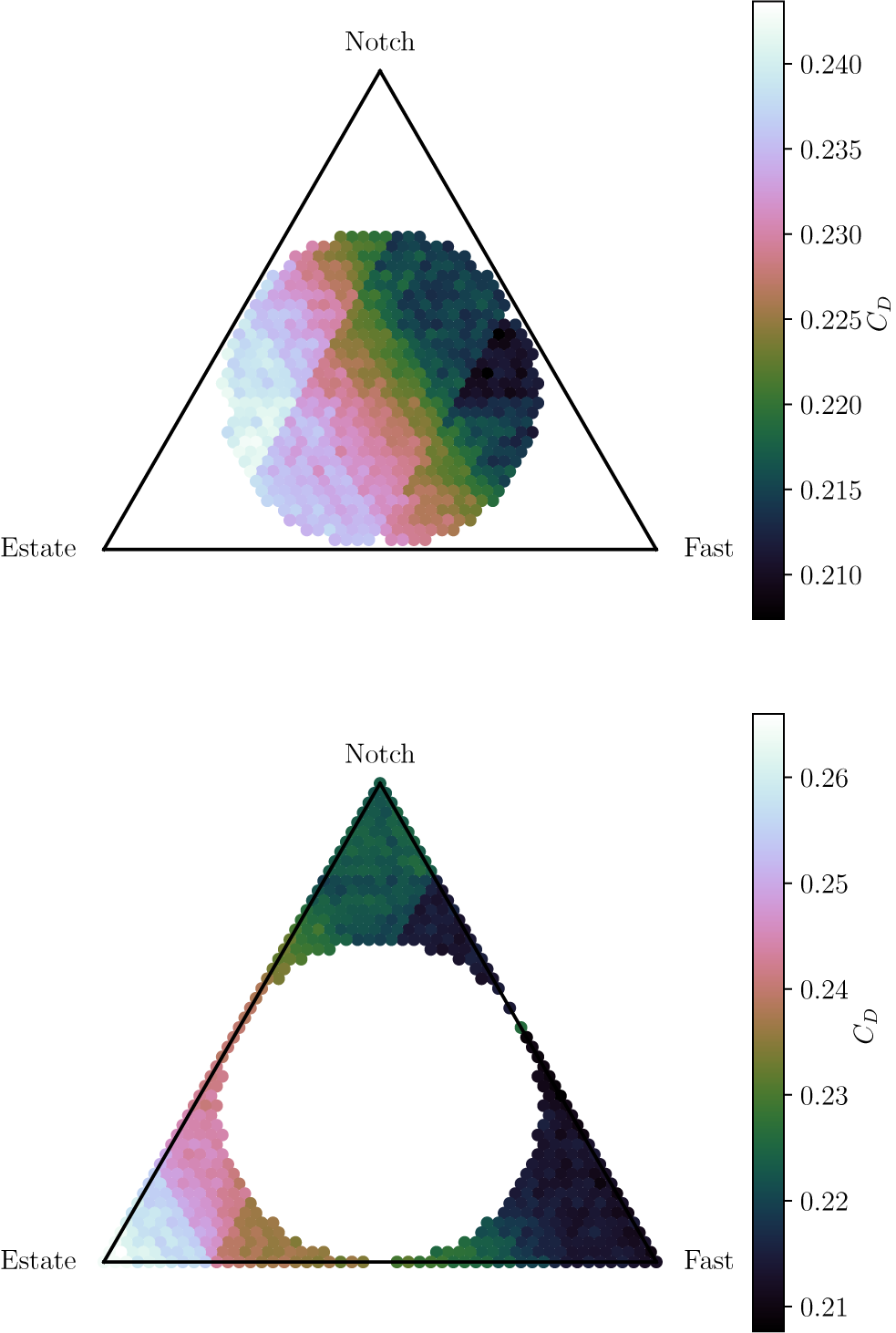

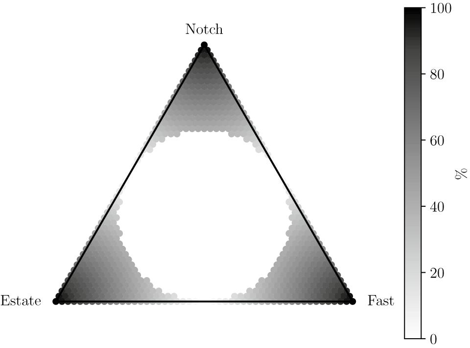
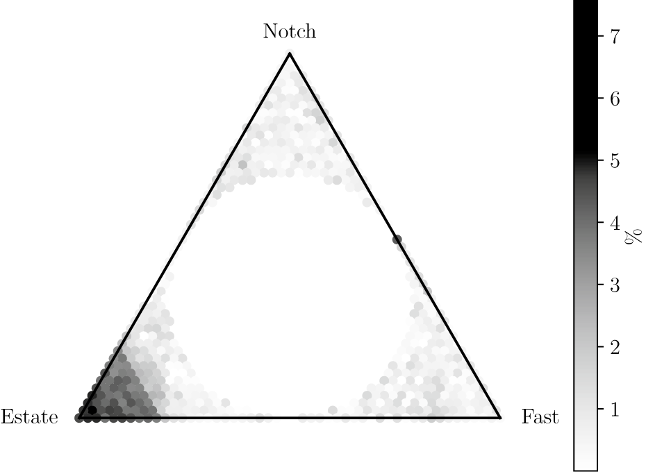
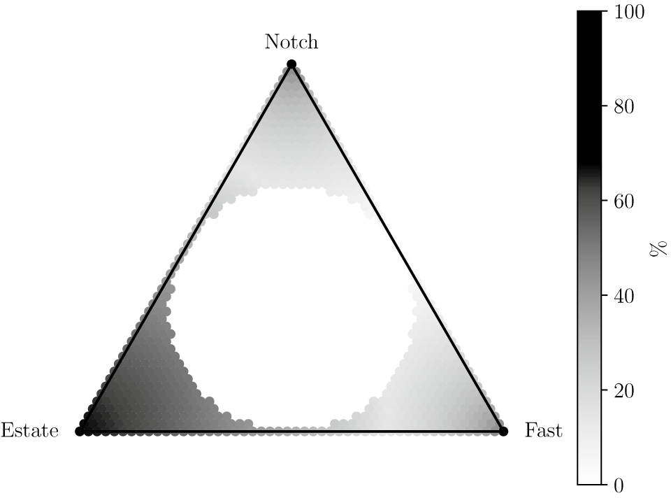
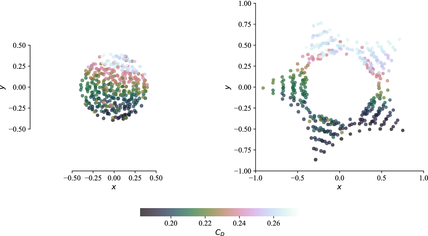


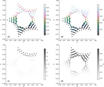


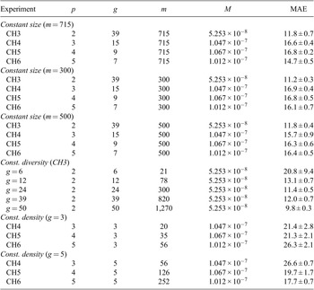
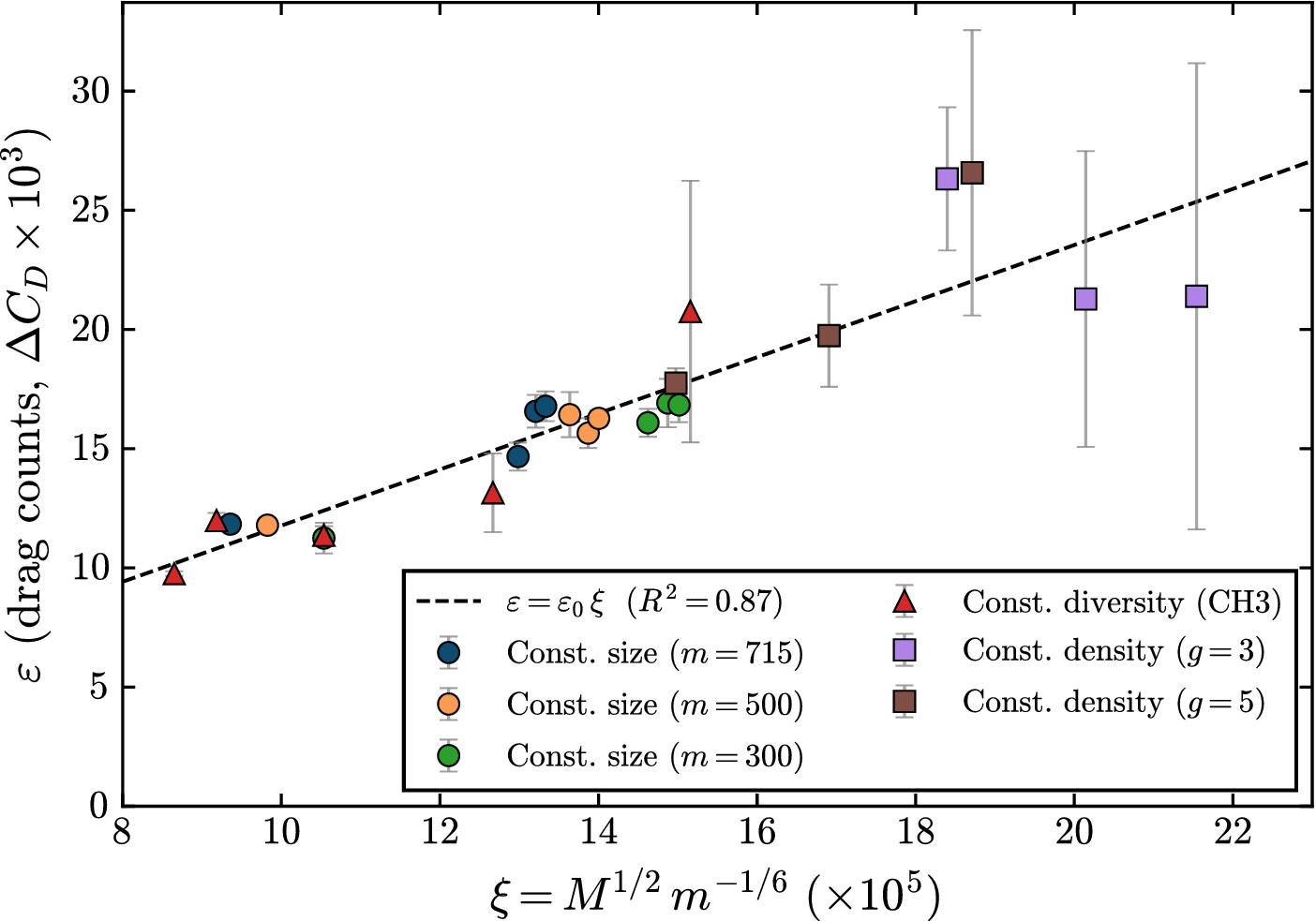


 Open access


Comments
No Comments have been published for this article.