


Impact Statement
Model Predictive Control (MPC) is one of the most impactful and promising technologies in the field of control. With the methods compared in this paper, it is possible to create a more accurate forward dynamics model by augmenting physics-based models with neural networks, from which MPC will benefit. On the example of a robot model corresponding to a challenging nonlinear system identification benchmark dataset, we present multiple hybrid model structures, combining physics-informed and data-driven models. This model collection equips the users with different exploratory opportunities and gives them additional insight for more educated choices on the model. Furthermore, our results confirm that using as much structural insight about the system as possible is important.
1. Introduction
Within the domain of physics-informed machine learning, the two disciplines of system identification and machine-learning converge at certain points, though each of these realms has its unique approaches and priorities. Practitioners of system identification, which is more closely associated with control systems, typically work with shorter datasets, focus on more compact models, and use substantial physical knowledge to build those models. Practitioners of machine learning, a field that has roots in computer science, typically focus on huge datasets and use universal approximators like artificial neural networks (ANNs).
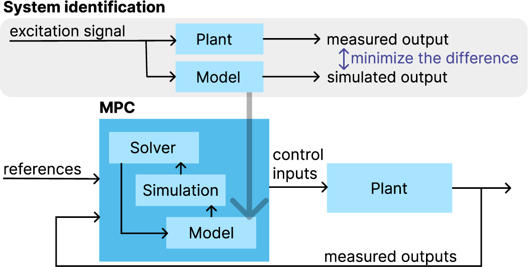
In this research, we aimed to create a high-fidelity simulation model of a robot arm for Model Predictive Control (MPC), as a more accurate model often leads to better tracking performance and a solution in fewer iterations. All aspects of a system’s behavior cannot be perfectly modeled using physical laws alone because of the measurement noise and those more complex nonlinear behaviors that are infeasible to model manually. However, we can still refine our model through machine-learning techniques that allow us to capture and predict these missing complex behaviors based on the data. In our case, we require an accurate prediction of the movement of the arm for given actuator torque inputs over a given finite time window ahead. In robotic MPC applications, this window is typically between 100 milliseconds (e.g., Zhao et al., Reference Zhao, Zhang, Ding, Tao and Ding2023) and 1 second (e.g., Trimble et al., Reference Trimble, Naeem, McLoone and Sopasakis2020). An overview of the connection between MPC and system identification for our use case is presented in Figure 1.
High-level overview of how the identified model will be used.
To achieve the highest possible accuracy, we evaluate a set of physics-based models augmented with ANNs in different ways. In general, physics-only models are fully explainable through the physical relations that govern the system, though they usually provide a lower accuracy. ANN-based models can often fit very well to the data but fail to extrapolate well on data in a range unseen during training (as described, for example, in Zhang and Cross, Reference Zhang, Cross, Madarshahian and Hemez2022). Furthermore, ANNs are rarely physically explainable. This lack of generalization calls for combinations of ANN and physics-based models, from which we expect better accuracy compared to a physics-only model and better explainability and extrapolation capability compared to an ANN-only model. Out of these metrics, the accuracy of simulations within a given time window ahead is evaluated in this work, as it is the most relevant to MPC. Given the computational complexity of calculating these N-step-ahead predictions, one of our research questions is if we can avoid calculating them during the training and validation steps. Instead, we use an indirect metric that is easier to compute, but our target is that the final model still reaches a good result on the N-step-ahead predictions.
This application-oriented benchmark study is organized as follows: a literature review of existing methods (Section 1.1) is in the remaining part of the introduction, along with the description of the plant (Section 1.2), the benchmark dataset (Section 1.3) and the physics-based model (Section 1.4): all the elements that were at our disposal at the beginning of this work. Afterward, all the details of our method are unraveled (Section 2): the augmented models that we compare (Section 2.1), the way of evaluation (Section 2.2), the objective function (Section 2.3), and the neural network implementation details (Section 2.4). Ultimately, the paper culminates in presenting the results (Section 3), their discussion (Section 4), and the conclusions (Section 5).
1.1. Related work and background
Models of electromechanical systems for prediction over a finite time window have been a long-standing research focus. Based on physical interpretability, Schoukens and Ljung (Reference Schoukens and Ljung2019) define several shades for model structures, from pit-black to snow-white models, with snow-white being the completely theory- and knowledge-based model. In the realm of machine learning, the different physics-informed approaches to deep learning are on various points of this scale. Lutter (Reference Lutter2021) introduces a Differentiable Newton–Euler Algorithm (DiffNEA) that uses virtual parameters to keep all the physical parameters physically interpretable, combined with gradient-based optimization techniques typically used for machine learning. DiffNEA results in a wholly physical model that can be integrated with machine-learning approaches like reinforcement learning, keeping close to white-box approaches on the scale mentioned. It provides considerably good extrapolation capability and achieves physical interpretability through virtual parameters. Some of its friction models are related but, at specific points, different from the combined models in this work. Deep Lagrangian Networks (DeLaN), also introduced by Lutter (Reference Lutter2021), combine deep learning with Lagrangian mechanics to learn dynamical models that conserve energy, with no specific knowledge of the system. However, they are close to the black-box endpoint of the scale.
The general framework of Physics-Informed Neural Networks (PINN) introduced by Raissi et al. (Reference Raissi, Perdikaris and Karniadakis2019) features an ANN with a time input that can learn to provide a data-driven solution to partial differential equations. Extensions to this framework have emerged, with the ANN also having a control input: compared to the Runge–Kutta-Fehlberg (also known as “RK45”) integration of a physics-based model, Nicodemus et al. (Reference Nicodemus, Kneifl, Fehr and Unger2022) achieved a reduction in computational time in an MPC setting. Similarly, Lambert et al. (Reference Lambert, Wilcox, Zhang, Pister and Calandra2021) created long-term simulation models for MPC and reinforcement learning scenarios; both are close to the complete black-box side of the scale. In contrast to these techniques, our approach is close to the middle of the interpretability scale, as we calculate part of our model directly from physical relations.
Another similar approach is called Physics-Guided Neural Networks (PGNN), introduced by Daw et al. (Reference Daw, Karpatne, Watkins, Read and Kumar2022). They apply a physics inconsistency term in the loss function and different combinations of physics-based models and neural networks, some of which we also evaluate for our application.
In De Groote et al. (Reference De Groote, Kikken, Hostens, Van Hoecke and Crevecoeur2022), the so-called Neural Network Augmented Physics (NNAP) models were introduced, where the neural network is inserted into the physics-based model of a slider crank mechanism to account for unknown nonlinear phenomena (unknown load interaction, effect of spring, and additional nonlinear friction). Our work shares some similarities with this, though we are exploring and comparing multiple ways of combining neural networks and physical models.
1.2. The plant
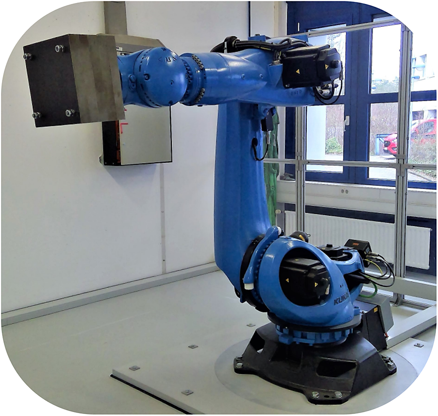
The system considered is a KUKA KR300 R2500 robot arm with six degrees of freedom, with a 150 kg mass attached to the end effector (see Figure 2). Its dynamics consist of the interaction of the robot’s rigid bodies, a contribution from a Hydraulic Weight Counterbalance (HWC) system installed on the second joint, and nonlinear friction. We expect additional nonlinearities from gearbox deformation and backlash.
The KUKA robot considered (image from Weigand et al., Reference Weigand, Götz, Ulmen and Ruskowski2022).
1.3. The data
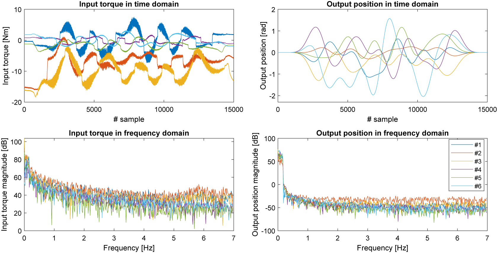
Weigand et al. (Reference Weigand, Götz, Ulmen and Ruskowski2022) made this system’s dataset available with corresponding input and output measurements. Their experiments were done in a closed loop; computed torque control (a proportional derivative controller operating in conjunction with the inverse dynamics) was applied to the machine to follow multisine trajectories designed to start from and end in zero angular position for all joints. Thirty-nine different trajectories have been executed, each of them twice, and the responses recorded. The recorded system outputs are the six joint angles. The recorded system inputs are the six motor torques. We show one of these trajectories in Figure 3. The sampling time is $ {T}_s=0.004 $
seconds, and the number of samples per trajectory is 15,000. A key observation is that as the angular positions follow the multisine reference trajectory well, so in the frequency domain, the position data indicates a very low level of leakage: as shown in Figure 3, we find that the magnitude drop after the last excited component is at least −40 dB.
$ {T}_s=0.004 $
seconds, and the number of samples per trajectory is 15,000. A key observation is that as the angular positions follow the multisine reference trajectory well, so in the frequency domain, the position data indicates a very low level of leakage: as shown in Figure 3, we find that the magnitude drop after the last excited component is at least −40 dB.
The training input–output data visualized in time domain (in full length) and frequency domain (from DC to 7 Hz).
1.4. The physics-based model
The physics-based model of the robot is a nonlinear state-space model with 12 states in total: angular positions ( $ x\in {\unicode{x211D}}^6 $
) and angular velocities (
$ x\in {\unicode{x211D}}^6 $
) and angular velocities ( $ v\in {\unicode{x211D}}^6 $
). It is composed of the
$ v\in {\unicode{x211D}}^6 $
). It is composed of the $ {f}_{\mathrm{fwd}} $
forward dynamics model of the robot, which relates the joint acceleration vector
$ {f}_{\mathrm{fwd}} $
forward dynamics model of the robot, which relates the joint acceleration vector $ a $
to the state vector
$ a $
to the state vector $ \left[x,v\right] $
, the input motor torque vector
$ \left[x,v\right] $
, the input motor torque vector $ {\tau}_{\mathrm{m}} $
and parameters
$ {\tau}_{\mathrm{m}} $
and parameters $ \theta $
:
$ \theta $
:
 $$ {f}_{\mathrm{rhs}}\left(x,v,{\tau}_{\mathrm{m}},\theta \right)=\left[\begin{array}{l}\dot{x}\\ {}\dot{v}\end{array}\right]=\left[\begin{array}{c}v\\ {}{f}_{\mathrm{fwd}}\left(x,v,{\tau}_{\mathrm{m}},\theta \right)\end{array}\right]. $$
We are integrating this model using the Runge–Kutta (RK4) method: $ {f}_{\mathrm{next}} $
is the resulting function that tells the state at the next discrete-time instant based on the current state, a fixed
$ {f}_{\mathrm{next}} $
is the resulting function that tells the state at the next discrete-time instant based on the current state, a fixed $ {T}_s $
time step later. Applying
$ {T}_s $
time step later. Applying $ {f}_{\mathrm{next}} $ $ k $
-times will result in a k-step long simulation
$ k $
-times will result in a k-step long simulation
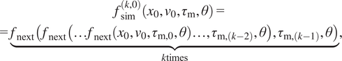 $$ {\displaystyle \begin{array}{c}{f}_{\mathrm{sim}}^{\left(k,0\right)}\left({x}_0,{v}_0,{\tau}_{\mathrm{m}},\theta \right)=\\ {}=\underset{k\mathrm{times}}{\underbrace{f_{\mathrm{next}}\left(\hskip0.15em ,{f}_{\mathrm{next}}\left(\dots {f}_{\mathrm{next}}\left({x}_0,{v}_0,{\tau}_{\mathrm{m},0},\theta \right)\dots, {\tau}_{\mathrm{m},\left(k-2\right)},\theta \right),{\tau}_{\mathrm{m},\left(k-1\right)},\theta \right)}},\end{array}} $$
with $ {x}_0 $
and
$ {x}_0 $
and $ {v}_0 $
corresponding to the initial positions and velocities, together with the initial state of the simulation, and
$ {v}_0 $
corresponding to the initial positions and velocities, together with the initial state of the simulation, and $ {\tau}_{\mathrm{m},j} $
as the column vector corresponding to the j
th time step in the motor torque matrix. We can define a simulation that starts from the p
th time instant instead of the zeroth as
$ {\tau}_{\mathrm{m},j} $
as the column vector corresponding to the j
th time step in the motor torque matrix. We can define a simulation that starts from the p
th time instant instead of the zeroth as
 $$ {\displaystyle \begin{array}{c}{f}_{\mathrm{sim}}^{\left(k,p\right)}\left({x}_p,{v}_p,{\tau}_{\mathrm{m}},\theta \right)=\\ {}=\underset{k\mathrm{times}}{\underbrace{f_{\mathrm{next}}\left({f}_{\mathrm{next}}\left(\dots {f}_{\mathrm{next}}\left({x}_p,{v}_p,{\tau}_{\mathrm{m},\mathrm{p}},\theta \right)\dots, {\tau}_{\mathrm{m},\left(p+k-2\right)},\theta \right),{\tau}_{\mathrm{m},\left(p+k-1\right)},\theta \right).}}\end{array}} $$
For the pure physical model, we choose $ {f}_{\mathrm{fwd}}={f}_{\mathrm{phy}} $
, and define the continuous-time model of the robot as
$ {f}_{\mathrm{fwd}}={f}_{\mathrm{phy}} $
, and define the continuous-time model of the robot as
 $$ {f}_{\mathrm{phy}}\left(x,v,\left[{\theta}_{\mathrm{in}}{\theta}_{\mathrm{f}}\right]\right)=a={\mathbf{M}}^{-1}\left(x,{\theta}_{\mathrm{in}}\right)\left(-\mathbf{C}\left(x,v,{\theta}_{\mathrm{in}}\right)\cdot v-g\left(x,{\theta}_{\mathrm{in}}\right).-.{\tau}_{\mathrm{f}}\left(v,{\theta}_{\mathrm{f}}\right)-{\tau}_{\mathrm{hwc}}(x)+u{\tau}_{\mathrm{m}}\right), $$
with $ \mathbf{M}\left(x,{\theta}_{\mathrm{in}}\right) $
as the inertia matrix,
$ \mathbf{M}\left(x,{\theta}_{\mathrm{in}}\right) $
as the inertia matrix, $ \mathbf{C}\left(x,v,{\theta}_{\mathrm{in}}\right) $
as the matrix corresponding to Coriolis and centripetal forces,
$ \mathbf{C}\left(x,v,{\theta}_{\mathrm{in}}\right) $
as the matrix corresponding to Coriolis and centripetal forces, $ g\left(x,{\theta}_{\mathrm{in}}\right) $
as the gravity vector,
$ g\left(x,{\theta}_{\mathrm{in}}\right) $
as the gravity vector, $ u $
as the vector of motor gear ratios,
$ u $
as the vector of motor gear ratios, $ {\tau}_{\mathrm{f}} $
as the friction torque vector,
$ {\tau}_{\mathrm{f}} $
as the friction torque vector, $ {\tau}_{\mathrm{hwc}} $
as the HWC torque vector.
$ {\tau}_{\mathrm{hwc}} $
as the HWC torque vector. $ {\theta}_{\mathrm{in}} $
are the inertial parameters,
$ {\theta}_{\mathrm{in}} $
are the inertial parameters, $ {\theta}_{\mathrm{f}} $
are the friction parameters.
$ {\theta}_{\mathrm{f}} $
are the friction parameters.
The friction is defined as
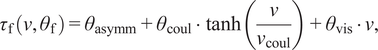 $$ {\tau}_{\mathrm{f}}\left(v,{\theta}_{\mathrm{f}}\right)={\theta}_{\mathrm{asymm}}+{\theta}_{\mathrm{coul}}\cdot \tanh \left(\frac{v}{v_{\mathrm{coul}}}\right)+{\theta}_{\mathrm{vis}}\cdot v, $$
with $ {\theta}_{\mathrm{asymm}} $
as the asymmetric friction component,
$ {\theta}_{\mathrm{asymm}} $
as the asymmetric friction component, $ {\theta}_{\mathrm{coul}}\cdot \tanh \left(\frac{v}{v_{\mathrm{coul}}}\right) $
as the Coulomb friction with the steepness of the tanh function chosen as
$ {\theta}_{\mathrm{coul}}\cdot \tanh \left(\frac{v}{v_{\mathrm{coul}}}\right) $
as the Coulomb friction with the steepness of the tanh function chosen as $ {v}_{coul}=1\frac{\mathrm{rad}}{\sec } $
, and
$ {v}_{coul}=1\frac{\mathrm{rad}}{\sec } $
, and $ {\theta}_{\mathrm{vis}}\cdot v $
as the viscous friction. The parameter vectors
$ {\theta}_{\mathrm{vis}}\cdot v $
as the viscous friction. The parameter vectors $ {\theta}_{\mathrm{asymm}},{\theta}_{\mathrm{coul}},{\theta}_{\mathrm{vis}}\in {\unicode{x211D}}^6 $
are grouped into
$ {\theta}_{\mathrm{asymm}},{\theta}_{\mathrm{coul}},{\theta}_{\mathrm{vis}}\in {\unicode{x211D}}^6 $
are grouped into $ {\theta}_{\mathrm{f}}=\left[{\theta}_{\mathrm{asymm}},{\theta}_{\mathrm{coul}},{\theta}_{\mathrm{vis}}\right]. $
As seen from (5),
$ {\theta}_{\mathrm{f}}=\left[{\theta}_{\mathrm{asymm}},{\theta}_{\mathrm{coul}},{\theta}_{\mathrm{vis}}\right]. $
As seen from (5), $ {\tau}_{\mathrm{f}} $
is linear in the parameters.
$ {\tau}_{\mathrm{f}} $
is linear in the parameters.
The model of the HWC is explained in detail in Weigand et al. (Reference Weigand, Götz, Ulmen and Ruskowski2022, p. 15). To summarize, $ {\tau}_{\mathrm{hwc}} $
only depends on the position of the second joint; its output torque only applies to that joint, and we consider the constants inside that model fixed throughout this work.
$ {\tau}_{\mathrm{hwc}} $
only depends on the position of the second joint; its output torque only applies to that joint, and we consider the constants inside that model fixed throughout this work.
The expressions for $ \mathbf{M}\left(x,{\theta}_{\mathrm{in}}\right),\mathbf{C}\left(x,v,{\theta}_{\mathrm{in}}\right),\mathbf{g}\left(x,{\theta}_{\mathrm{in}}\right) $
are acquired based on the Denavit–Hartenberg (DH) parameters of the robot, using the SymPyBotics toolbox of Sousa (Reference Sousa2014), through the recursive Newton–Euler method. The DH parameters input to SymPyBotics are listed in Table 1.
$ \mathbf{M}\left(x,{\theta}_{\mathrm{in}}\right),\mathbf{C}\left(x,v,{\theta}_{\mathrm{in}}\right),\mathbf{g}\left(x,{\theta}_{\mathrm{in}}\right) $
are acquired based on the Denavit–Hartenberg (DH) parameters of the robot, using the SymPyBotics toolbox of Sousa (Reference Sousa2014), through the recursive Newton–Euler method. The DH parameters input to SymPyBotics are listed in Table 1.
DH parameters of the KUKA KR300 R2500 robot arm concerned.

The formulas output by SymPyBotics are very complex and highly nonlinear with respect to both the state and the parameters. $ \mathbf{M},\mathbf{C},\mathbf{g} $
nonlinearly depend on the following 66 inertial parameters:
$ \mathbf{M},\mathbf{C},\mathbf{g} $
nonlinearly depend on the following 66 inertial parameters:
 $$ {\theta}_{\mathrm{in}}=\left[{L}_{i\mathrm{x}\mathrm{x}},{L}_{i\mathrm{x}\mathrm{y}},{L}_{i\mathrm{x}\mathrm{z}},{L}_{i\mathrm{y}\mathrm{y}},{L}_{i\mathrm{y}\mathrm{z}},{L}_{i\mathrm{z}\mathrm{z}},{l}_{i\mathrm{x}},{l}_{i\mathrm{y}},{l}_{i\mathrm{z}},{m}_i,{I}_{i\mathrm{a}}|\forall i\in \left\{1,\dots, 6\right\}\right], $$
with $ {m}_i $
as the link mass,
$ {m}_i $
as the link mass, $ {I}_{i\mathrm{a}} $
as the motor inertia,
$ {I}_{i\mathrm{a}} $
as the motor inertia, $ {l}_{i\mathrm{x}},{l}_{i\mathrm{y}},{l}_{i\mathrm{z}} $
as the first moments of inertia,
$ {l}_{i\mathrm{x}},{l}_{i\mathrm{y}},{l}_{i\mathrm{z}} $
as the first moments of inertia, $ {L}_{i\mathrm{xx}},{L}_{i\mathrm{xy}},{L}_{i\mathrm{xz}},{L}_{i\mathrm{yy}},{L}_{i\mathrm{yz}},{L}_{i\mathrm{zz}} $
as the elements of the inertia tensor of the link with respect to the center of mass, all corresponding to the i
th link. Aside from those discussed above, there could be additional nonlinearities from gearbox deformation and backlash, but these are not currently modeled.
$ {L}_{i\mathrm{xx}},{L}_{i\mathrm{xy}},{L}_{i\mathrm{xz}},{L}_{i\mathrm{yy}},{L}_{i\mathrm{yz}},{L}_{i\mathrm{zz}} $
as the elements of the inertia tensor of the link with respect to the center of mass, all corresponding to the i
th link. Aside from those discussed above, there could be additional nonlinearities from gearbox deformation and backlash, but these are not currently modeled.
We refer to the parameters of this physical model as $ {\theta}_{\mathrm{phy}}=\left[{\theta}_{\mathrm{in}},{\theta}_{\mathrm{f}}\right]. $
The initial values for inertia and friction parameters, from which we start the optimization, were identified in the preceding work by the authors and contributors of Weigand et al. (Reference Weigand, Götz, Ulmen and Ruskowski2022). The inertial parameters were estimated based on publicly available data of the robot and the components (e.g., gearboxes and drives): the available solid computer-aided design (CAD) models of the robotic arm were hollow cut, and the properties of the expected materials of the components were looked up, see the work of Harttig (Reference Harttig2018). The initial friction parameters were determined using global optimization based on the surrogate optimization algorithm of Regis and Shoemaker (Reference Regis and Shoemaker2007), available in MATLAB. As seen in Figure 8, the initial model is not adequate for simulation.
$ {\theta}_{\mathrm{phy}}=\left[{\theta}_{\mathrm{in}},{\theta}_{\mathrm{f}}\right]. $
The initial values for inertia and friction parameters, from which we start the optimization, were identified in the preceding work by the authors and contributors of Weigand et al. (Reference Weigand, Götz, Ulmen and Ruskowski2022). The inertial parameters were estimated based on publicly available data of the robot and the components (e.g., gearboxes and drives): the available solid computer-aided design (CAD) models of the robotic arm were hollow cut, and the properties of the expected materials of the components were looked up, see the work of Harttig (Reference Harttig2018). The initial friction parameters were determined using global optimization based on the surrogate optimization algorithm of Regis and Shoemaker (Reference Regis and Shoemaker2007), available in MATLAB. As seen in Figure 8, the initial model is not adequate for simulation.
There also exists another linear baseline model provided with the dataset in Weigand et al. (Reference Weigand, Götz, Ulmen and Ruskowski2022), though it is important to note that this model is even more limited due to the strong nonlinear nature of the robot forward dynamics.
2. The method
2.1. Augmenting the physics-based model with ANNs
To improve upon the physics-only model, we compare several ways to augment the physics-based model with ANNs, particularly with multilayer perceptrons (MLPs) that have a residual connection (an additional linear layer directly between the inputs and outputs). We have implemented normalization of the input and output features to standard deviation $ \sigma =1 $
and mean
$ \sigma =1 $
and mean $ \mu =0 $
, based on previous results discussed in Beintema et al. (Reference Beintema, Schoukens and Tóth2023). As mentioned there, weight initialization methods such as Glorot and Bengio (Reference Glorot and Bengio2010) assume normalized inputs and outputs. Input normalization is also discussed as an often-used technique in Aggarwal (Reference Aggarwal2018, p. 127). We have calculated the normalization factors from the data, considering the full model equations, using all the training, validation, and test datasets.
$ \mu =0 $
, based on previous results discussed in Beintema et al. (Reference Beintema, Schoukens and Tóth2023). As mentioned there, weight initialization methods such as Glorot and Bengio (Reference Glorot and Bengio2010) assume normalized inputs and outputs. Input normalization is also discussed as an often-used technique in Aggarwal (Reference Aggarwal2018, p. 127). We have calculated the normalization factors from the data, considering the full model equations, using all the training, validation, and test datasets.
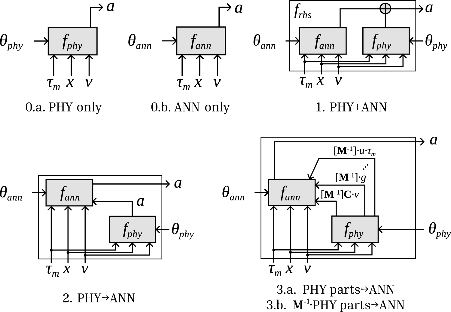
Below is a list of evaluated model structures. The formulas are listed in Table 2 and shown visually in Figures 4 and 5. We gave every model a name so that we could easily refer to them; along with the model numbers, these are mentioned in the figures and the table.
-
• Model 0.a “PHY-only” consists solely of the physics-based model.
-
• Model 0.b is the “ANN-only” model. It consists of a single MLP. It has the same 18 inputs (six positions, six velocities, and six motor torques) and six outputs (accelerations) as Model 0.a.
-
• In Model 1, “PHY + ANN”, the acceleration outputs of the ANN and the physical model are added together per channel. This is a residual model (called residual Hybrid-Physics-Data (HPD) model in Daw et al., Reference Daw, Karpatne, Watkins, Read and Kumar2022) for approximating an additional term that is missing from the physical model. For this model, we calculate the normalization factors of the neural network outputs based on the difference between the output of the physics-based model and the actual acceleration.
-
• In Model 2, “PHY $ \to $
ANN”, the output of the physics-based model, is an input to the neural network, along with the current state and motor torque. In this case, the role of the ANN is to “correct” the acceleration coming from the physics-based model, knowing all the inputs of that model as well. This is called a basic HPD model in Daw et al. (Reference Daw, Karpatne, Watkins, Read and Kumar2022).
$ \to $
ANN”, the output of the physics-based model, is an input to the neural network, along with the current state and motor torque. In this case, the role of the ANN is to “correct” the acceleration coming from the physics-based model, knowing all the inputs of that model as well. This is called a basic HPD model in Daw et al. (Reference Daw, Karpatne, Watkins, Read and Kumar2022). -
• In Model 3, the terms of the formula of the physics-based model are separately input to the ANN, along with the current state and motor torque. Under 3, we have two submodels: in 3.b “
$ {M}^{-1}\cdot $
PHY parts
$ \to $
ANN”; these terms contain the multiplication by
$ {\mathbf{M}}^{-1}\left(x,{\theta}_{\mathrm{in}}\right) $
, while in 3.a “PHY parts
$ \to $
ANN” this multiplication is omitted. The difference is the preprocessing applied to the input features, and our goal was to evaluate which one is more efficient, similar to De Groote et al. (Reference De Groote, Kikken, Hostens, Van Hoecke and Crevecoeur2022). Note that out of all these terms input to the ANN, some are always zero or close to zero. For example, in the vector
$ {\tau}_{\mathrm{hwc}} $
, only the second element is non-zero; the others are structurally zero. As these elements do not carry meaningful information, we omitted them, i.e., we did not input them to the ANN. -
• Model 4 “vel.
$ \to $
ANN per joint” draws inspiration from the understanding that the friction torque per joint mainly depends on the velocity of the given joint. Thus, we instantiate separate neural networks per joint (their parameter vectors are denoted by
$ {\theta}_{\mathrm{ann}1},\dots, {\theta}_{\mathrm{ann}6} $
). Each of these single-input, single-output (SISO) networks has the same structure concerning the number of layers and number of neurons. -
• Model 5 “(vel., all pos.)
$ \to $
ANN per joint” is very similar to Model 4, though we also input all the positions to each of these separate networks, resulting in seven inputs and a single-output per network. The idea behind this is that the load on the joint depends on the complete configuration of the machine, and we were expecting that the ANN could use the information in the position data.


Model structures
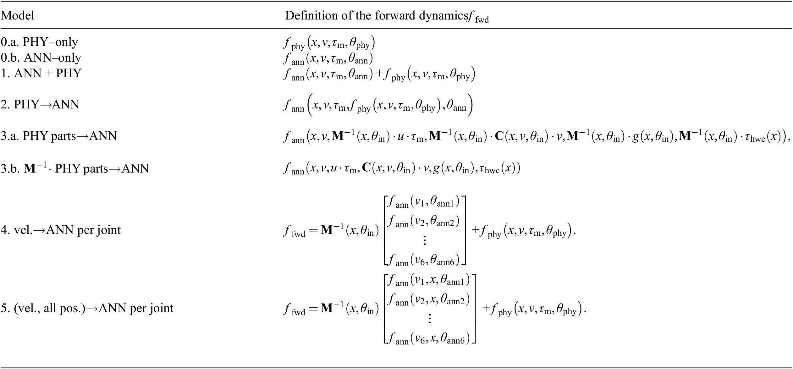
Combinations of physics-based and ANN models from 0.a to 3.
Combinations of physics-based and ANN models, 4 and 5.
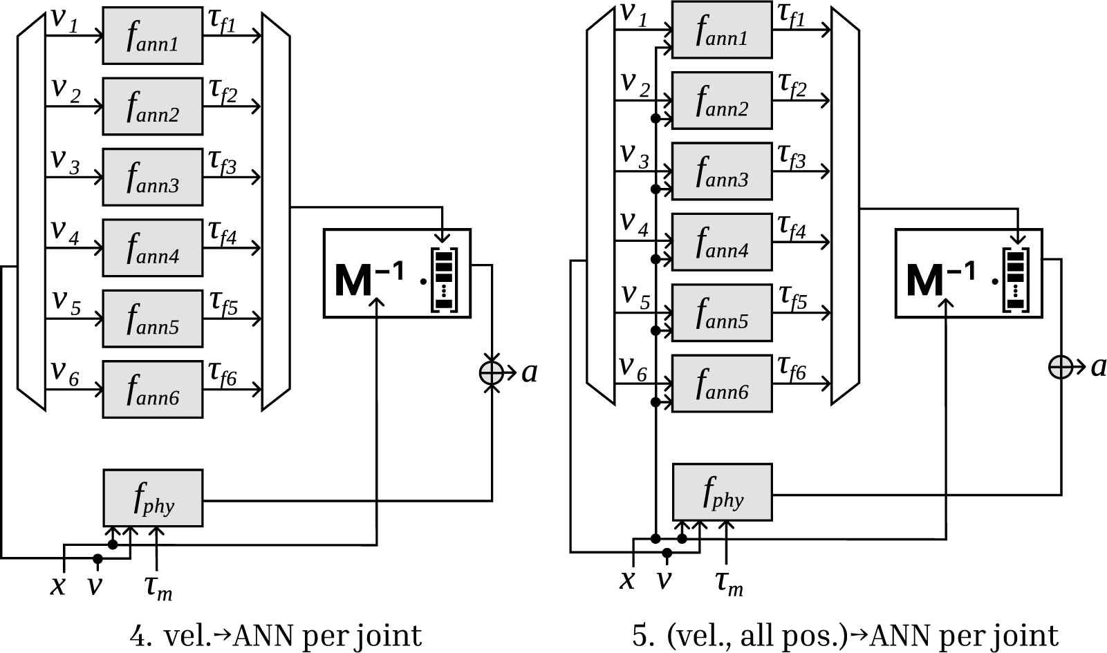
Models 0.a and 0.b represent the two endpoints of the scale with respect to explainability, and they serve as a baseline for the models described thereafter. Models 1–3 are general combinations of ANNs and physics-based models, constructed without physical insight and still fully capable of universal approximation. In Models 4 and 5, the configuration that follows the mechanical structure imposes a strong inductive bias. Aside from the 0.a “PHY-only” model, the friction term $ {\tau}_{\mathrm{f}} $
inside
$ {\tau}_{\mathrm{f}} $
inside $ {f}_{\mathrm{phy}} $
was not active in any other models, as including these friction terms did not result in model improvements in our experiments. We have yet to find Models 3.a, 3.b, and 5 in this exact way in the literature; thus, we consider them our contributions.
$ {f}_{\mathrm{phy}} $
was not active in any other models, as including these friction terms did not result in model improvements in our experiments. We have yet to find Models 3.a, 3.b, and 5 in this exact way in the literature; thus, we consider them our contributions.
2.2. Evaluation of the model: 150-step-NRMS
As stated before, our goal is to get the most accurate N-step-ahead simulation model for the robot. We evaluated the model on a 600-millisecond window, equivalent to 150 simulation steps, within the range typically used for MPC. The N-step-NRMS error measure, the normalized root mean square (NRMS) error with $ N=150 $
corresponds to this situation, as
$ N=150 $
corresponds to this situation, as $ 150\cdot {T}_s=0.6 $
second. We denote this measure with
$ 150\cdot {T}_s=0.6 $
second. We denote this measure with $ {\eta}_{150} $
, and as a note, the same error measure also appears in Beintema et al. (Reference Beintema, Tóth and Schoukens2021, p. 4) and Weigand et al. (Reference Weigand, Götz, Ulmen and Ruskowski2022). It is calculated as follows:
$ {\eta}_{150} $
, and as a note, the same error measure also appears in Beintema et al. (Reference Beintema, Tóth and Schoukens2021, p. 4) and Weigand et al. (Reference Weigand, Götz, Ulmen and Ruskowski2022). It is calculated as follows:
 $$ {\eta}_{\left({N}_{\mathrm{steps}}\right)}={\left\{\sum \limits_{p=1}^{N_{\mathrm{starts}}}\sum \limits_{k=1}^{N_{\mathrm{steps}}}{\left\Vert \operatorname{diag}\left(\frac{1}{\sigma_{\mathrm{p}}}\right)\cdot \left[{f}_{\mathrm{sim}}^{\left(k,p\right)}{\left({x}_{\mathrm{filt},p},{v}_{\mathrm{dx},p},{\tau}_{\mathrm{m},\mathrm{filt}},\theta \right)}_{\left[1:6\right]}-{x}_{\mathrm{filt},\left(p+k\right)}\right]\right\Vert}_2^2\right\}}^{\frac{1}{2}}, $$
with $ {\tau}_{\mathrm{m},\mathrm{filt}} $
,
$ {\tau}_{\mathrm{m},\mathrm{filt}} $
, $ {x}_{\mathrm{filt}} $
, and
$ {x}_{\mathrm{filt}} $
, and $ {v}_{\mathrm{dx}} $
as the filtered motor torques, positions, and the velocities calculated from the positions, respectively,
$ {v}_{\mathrm{dx}} $
as the filtered motor torques, positions, and the velocities calculated from the positions, respectively, $ {\sigma}_{\mathrm{p}} $
as the vector of standard deviations of each channel of
$ {\sigma}_{\mathrm{p}} $
as the vector of standard deviations of each channel of $ {x}_{\mathrm{filt}} $
, and
$ {x}_{\mathrm{filt}} $
, and $ {N}_{\mathrm{steps}}=N $
as the number of simulation steps in N-step-NRMS,
$ {N}_{\mathrm{steps}}=N $
as the number of simulation steps in N-step-NRMS, $ {N}_{\mathrm{starts}} $
as the number of starting positions. The filtered signals are calculated in the frequency domain as
$ {N}_{\mathrm{starts}} $
as the number of starting positions. The filtered signals are calculated in the frequency domain as
 $$ {\displaystyle \begin{array}{c}{x}_{\mathrm{filt}}={\mathrm{F}}^{-1}\left(h\left(\mathrm{F}\left({x}_{\mathrm{m}\mathrm{eas}}\right)\right)\right),\\ {}{v}_{\mathrm{dx}}={\mathrm{F}}^{-1}\left(- j\omega \cdot h\left(\mathrm{F}\left({x}_{\mathrm{m}\mathrm{eas}}\right)\right)\right),\\ {}{\tau}_{\mathrm{m},\mathrm{filt}}={\mathrm{F}}^{-1}\left(h\left(\mathrm{F}\left({\tau}_{\mathrm{m},\mathrm{meas}}\right)\right)\right),\\ {}h(x)=\left\{\begin{array}{cc}{x}_i& \mid \hskip0.15em i\le 200,\\ {}0& \mid \hskip0.15em i>200,\end{array}\right.\end{array}} $$
where $ h(x) $
is our filter,
$ h(x) $
is our filter, $ \mathrm{F} $
denotes the Fourier-transform,
$ \mathrm{F} $
denotes the Fourier-transform, $ {\mathrm{F}}^{-1} $
indicates the inverse Fourier-transform,
$ {\mathrm{F}}^{-1} $
indicates the inverse Fourier-transform, $ {\tau}_{\mathrm{m},\mathrm{meas}} $
and
$ {\tau}_{\mathrm{m},\mathrm{meas}} $
and $ {x}_{\mathrm{meas}} $
represent the measured motor torques and joint positions, respectively, and
$ {x}_{\mathrm{meas}} $
represent the measured motor torques and joint positions, respectively, and $ \omega $
stands for the angular frequency corresponding to each bin inside the frequency domain signal. The FFT is used in the implementation of
$ \omega $
stands for the angular frequency corresponding to each bin inside the frequency domain signal. The FFT is used in the implementation of $ \mathrm{F} $
and
$ \mathrm{F} $
and $ {\mathrm{F}}^{-1} $
. When calculating derivatives of noisy data, the filtering operation is necessary to remove the high-frequency noise that the differentiation would otherwise emphasize.
$ {\mathrm{F}}^{-1} $
. When calculating derivatives of noisy data, the filtering operation is necessary to remove the high-frequency noise that the differentiation would otherwise emphasize.
As seen from (7), $ {\eta}_{150} $
is a unitless proportion (the unit of the error between the simulation and the filtered measurement is either rad or rad/s, but we divide it by the standard deviation of the filtered measurement which has the same unit). The higher value indicates a higher discrepancy between simulation and measurement.
$ {\eta}_{150} $
is a unitless proportion (the unit of the error between the simulation and the filtered measurement is either rad or rad/s, but we divide it by the standard deviation of the filtered measurement which has the same unit). The higher value indicates a higher discrepancy between simulation and measurement.
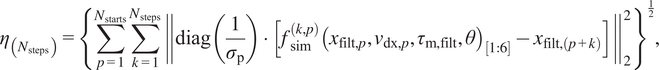
The explanation of (7) is as follows. Given $ N={N}_{\mathrm{steps}}=150 $
simulation steps to take into account, we calculate simulations from all possible starting positions, meaning that if we have 15,000 samples, then we start from
$ N={N}_{\mathrm{steps}}=150 $
simulation steps to take into account, we calculate simulations from all possible starting positions, meaning that if we have 15,000 samples, then we start from $ {N}_{\mathrm{starts}}=15000-150=14850 $
different time steps, and calculate a forward simulation of 150 steps from each of them. Figure 6 shows this concept. As a result, we gain a three-dimensional array with dimensions
$ {N}_{\mathrm{starts}}=15000-150=14850 $
different time steps, and calculate a forward simulation of 150 steps from each of them. Figure 6 shows this concept. As a result, we gain a three-dimensional array with dimensions $ \left[{N}_{\mathrm{steps}},{N}_{\mathrm{starts}},{N}_{\mathrm{channels}}\right] $
with
$ \left[{N}_{\mathrm{steps}},{N}_{\mathrm{starts}},{N}_{\mathrm{channels}}\right] $
with $ {N}_{\mathrm{channels}}=12 $
as the number of states. Then we calculate the average of each of the squared errors between the simulated and measured states along the dimensions corresponding to the steps and starting positions, weighting the channels by
$ {N}_{\mathrm{channels}}=12 $
as the number of states. Then we calculate the average of each of the squared errors between the simulated and measured states along the dimensions corresponding to the steps and starting positions, weighting the channels by $ \frac{1}{\sigma_{\mathrm{p}}} $
, to get a single number for the loss ultimately. Unfortunately, the initial physics-only Model 0.a evaluated this way shows a considerably high mismatch with the data, as seen in Figure 8.
$ \frac{1}{\sigma_{\mathrm{p}}} $
, to get a single number for the loss ultimately. Unfortunately, the initial physics-only Model 0.a evaluated this way shows a considerably high mismatch with the data, as seen in Figure 8.
Illustration of calculating the N-step-NRMS (7).
2.3. Objective: acceleration-based error measure
While we use the 150-step-NRMS error measure to evaluate the model, unfortunately, it is computationally costly. Instead, we applied an acceleration-based error measure during the training and validation steps: in those steps, the error must be recalculated in every epoch. We then applied a 150-step-NRMS error measure in the test phase afterward, which was calculated only once.
The simulation, implemented in PyTorch from Paszke et al. (Reference Paszke2019) becomes very slow once the physics-based model is applied. As an example, calculating the 150-step-ahead simulation from all the possible places with Model 3.a takes approximately 77 seconds on a computer with 10 CPU cores available. Applying the GPU acceleration and the Just-In-Time (JIT) compilation functionality built into PyTorch did not improve the overall speed, probably because the operations carried out are sequential and not suitable for the JIT fuser.
We solved the computational complexity in the following way: the output of the continuous-time model $ {f}_{\mathrm{fwd}} $
is one acceleration per joint, so we fit these to the six accelerations calculated from the measured positions. Such an error measure is described, for example, in Lutter (Reference Lutter2021, p. 9, (2.2)). In this case, we observe that the 15,000-sample measured position trajectories result in a periodic signal. As a result, we can calculate the derivative of the positions in the frequency domain, resulting in velocity and acceleration signals, as already seen in (8). However, this differentiation acts as a high-pass filter on the signal, emphasizing the noise on the higher frequencies. We observe that in the frequency domain, the position signal does not contain meaningful information above approximately 6 Hz, so we weight the frequency data with a rectangular window, zeroing all content corresponding to frequencies above the 200th bin that corresponds to the frequency mentioned before, equivalent to applying an ideal low-pass filter. As seen in (8), we are also applying the filter to the torques
$ {f}_{\mathrm{fwd}} $
is one acceleration per joint, so we fit these to the six accelerations calculated from the measured positions. Such an error measure is described, for example, in Lutter (Reference Lutter2021, p. 9, (2.2)). In this case, we observe that the 15,000-sample measured position trajectories result in a periodic signal. As a result, we can calculate the derivative of the positions in the frequency domain, resulting in velocity and acceleration signals, as already seen in (8). However, this differentiation acts as a high-pass filter on the signal, emphasizing the noise on the higher frequencies. We observe that in the frequency domain, the position signal does not contain meaningful information above approximately 6 Hz, so we weight the frequency data with a rectangular window, zeroing all content corresponding to frequencies above the 200th bin that corresponds to the frequency mentioned before, equivalent to applying an ideal low-pass filter. As seen in (8), we are also applying the filter to the torques $ {\tau}_{\mathrm{m},\mathrm{meas}} $
, though the torque signal is not periodic, thus we will get a slight spectral leakage due to the discontinuity.
$ {\tau}_{\mathrm{m},\mathrm{meas}} $
, though the torque signal is not periodic, thus we will get a slight spectral leakage due to the discontinuity.
We define the $ {a}_{\mathrm{ddx}} $
filtered accelerations and the
$ {a}_{\mathrm{ddx}} $
filtered accelerations and the $ \zeta $
acceleration-based error measure as
$ \zeta $
acceleration-based error measure as
 $$ {\displaystyle \begin{array}{c}{a}_{\mathrm{ddx}}={\mathrm{F}}^{-1}\left({\omega}^2\cdot h\left(\mathrm{F}\left({x}_{\mathrm{m}\mathrm{eas}}\right)\right)\right),\\ {}\zeta ={\left\Vert \operatorname{diag}\left(\frac{1}{\sigma_{\mathrm{a}}}\right)\cdot \left[{a}_{\mathrm{ddx}}-{f}_{\mathrm{fwd}}\left({x}_{\mathrm{filt}},{v}_{\mathrm{dx}},{\tau}_{\mathrm{m},\mathrm{filt}},\theta \right)\right]\right\Vert}_2^2,\end{array}} $$
with $ {\sigma}_{\mathrm{a}} $
as the standard deviation corresponding to each channel in
$ {\sigma}_{\mathrm{a}} $
as the standard deviation corresponding to each channel in $ {a}_{\mathrm{ddx}} $
.
$ {a}_{\mathrm{ddx}} $
.
Indeed, we can only use (9) if our system only has states that correspond to positions that are measurable and states that correspond to velocities that can be inferred from the positions. When calculating velocities or accelerations is needed, it is common to calculate it through finite differences (see, e.g., Lutter, Reference Lutter2021, p. 50). The formulation in (9) is an alternative to this.
2.4. Neural network and optimization details
We use the Adaptive Moment Estimation (ADAM) optimization algorithm of Kingma and Ba (Reference Kingma and Ba2015), which has recently become a typical default choice in deep learning, to update the ANN weights or the physics-based model parameters.
We use a standard procedure for data partitioning: three different periods as training, validation, and test datasets. The training set is used to adjust the model parameters in every epoch. The validation set is also used during training to provide an unbiased model evaluation and mitigate the risk of overfitting. It is used in early stopping: the optimization is terminated if the validation loss does not demonstrate an improvement over 1000 epochs while training the ANN. Finally, after the training phase, we use the test set for an unbiased evaluation of the performance of the final models. The test set also allows us to verify the extrapolation performance concerning robot poses unseen during training.
As a note, we break down our training phase into two steps. First, we optimize the physical model parameters $ {\theta}_{\mathrm{phy}} $
over the course of 5000 epochs, during which only
$ {\theta}_{\mathrm{phy}} $
over the course of 5000 epochs, during which only $ {f}_{\mathrm{phy}} $
is active (i.e., replaces
$ {f}_{\mathrm{phy}} $
is active (i.e., replaces $ {f}_{\mathrm{fwd}} $
in the objective). Additionally, we disable early stopping to prevent it from being triggered during this period. Second, we optimize only the ANN parameters
$ {f}_{\mathrm{fwd}} $
in the objective). Additionally, we disable early stopping to prevent it from being triggered during this period. Second, we optimize only the ANN parameters $ {\theta}_{\mathrm{ann}} $
, and the entire
$ {\theta}_{\mathrm{ann}} $
, and the entire $ {f}_{\mathrm{fwd}} $
(with both physical and ANN parts, when applicable) is active until early stopping is triggered. The first step makes the physical model more accurate before using its information in the combined models in the second step.
$ {f}_{\mathrm{fwd}} $
(with both physical and ANN parts, when applicable) is active until early stopping is triggered. The first step makes the physical model more accurate before using its information in the combined models in the second step.
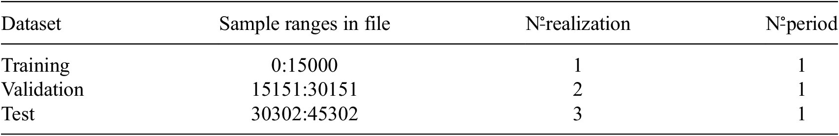
The data file used was recording_2021_12_15_20H_45M.mat from Weigand et al. (Reference Weigand, Götz, Ulmen and Ruskowski2022), and the training, validation, and test data are concretely described in Table 3. The software stack we used to implement this is the deepSI framework from Beintema et al. (Reference Beintema, Tóth and Schoukens2021), which is based on PyTorch.
Data selected from py_recording_2021_12_15_20H_45M.mat for use in this work.
The neural network we apply has 1000 neurons per layer, two hidden layers, a residual connection, and tanh activation function. Models 4 and 5 are exceptions to this, with 100 neurons per layer, but then with six separate, small networks (one per joint) instead of one large. We apply regularization to the ANN parameters by the weight decay built into the implementation of the ADAM solver. We applied hyperparameter tuning to find the right choice for the weight decay. We have been manually tuning the learning rate of ADAM to find a value that is large enough but does not result in strong fluctuations in the training loss. This value is $ {10}^{-4} $
for
$ {10}^{-4} $
for $ {\theta}_{\mathrm{ann}} $
and
$ {\theta}_{\mathrm{ann}} $
and $ 1.0 $
for
$ 1.0 $
for $ {\theta}_{\mathrm{phy}} $
: we apply different learning rates to the two sets of parameters. Because of these different learning rates for the two components of the model and the need to balance them well, optimizing
$ {\theta}_{\mathrm{phy}} $
: we apply different learning rates to the two sets of parameters. Because of these different learning rates for the two components of the model and the need to balance them well, optimizing $ {\theta}_{\mathrm{phy}} $
and
$ {\theta}_{\mathrm{phy}} $
and $ {\theta}_{\mathrm{ann}} $
together is difficult. We have decided not to optimize them in the same step. The weight initialization corresponds to the default uniform initialization provided by deepSI and PyTorch.
$ {\theta}_{\mathrm{ann}} $
together is difficult. We have decided not to optimize them in the same step. The weight initialization corresponds to the default uniform initialization provided by deepSI and PyTorch.
2.5. Cases
The interaction between surfaces is complex, and we can differentiate between different types of friction based on the phenomenon observed, e.g., static, presliding, sliding, or stick–slip friction. Using this insight, we have been considering two cases for the experiments:
-
• in Case 1, the models are evaluated on the complete trajectories (one trajectory for training, validation, and test each),
-
• in Case 2, the models are evaluated on reduced trajectories (the first and last 1350 samples are left out). The reason for reducing the trajectories is to eliminate regions where the velocity is consistently very low, where the effects of the difficult-to-model presliding friction are strongest.
3. Results
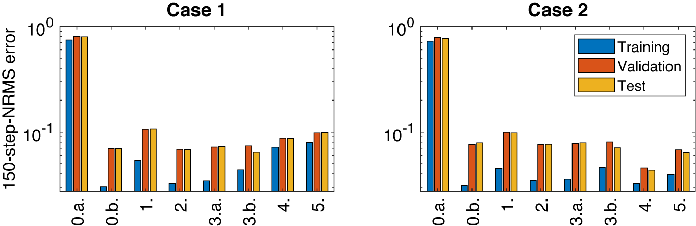
In Table 4, the results corresponding to the two cases are listed. The lower value corresponds to better accuracy, meaning a lower error between the simulation and the data. Only the results on the test dataset are reported in the table, but we also provide a visualization of the results on graphs in Figure 7, which show the 150-step-NRMS on the training and validation sets. These results are after the hyperparameter tuning: we have made a few trials to adjust the weight decay to find the lowest 150-step-NRMS on the validation data.
Comparison of models across Cases 1 and 2.
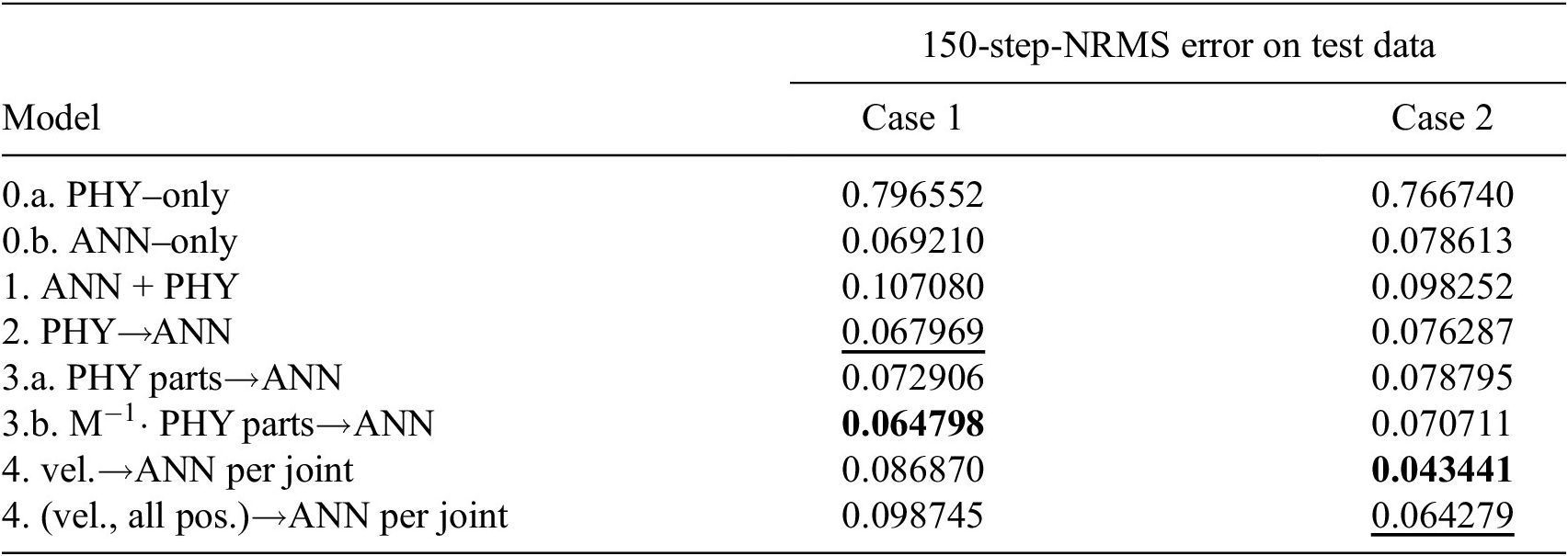
Note. The best result per case is formatted in bold, the second best result is indicated with an underline.
Results from Table 4 on a bar graph: 150-step-NRMS error on training, validation, and test data.
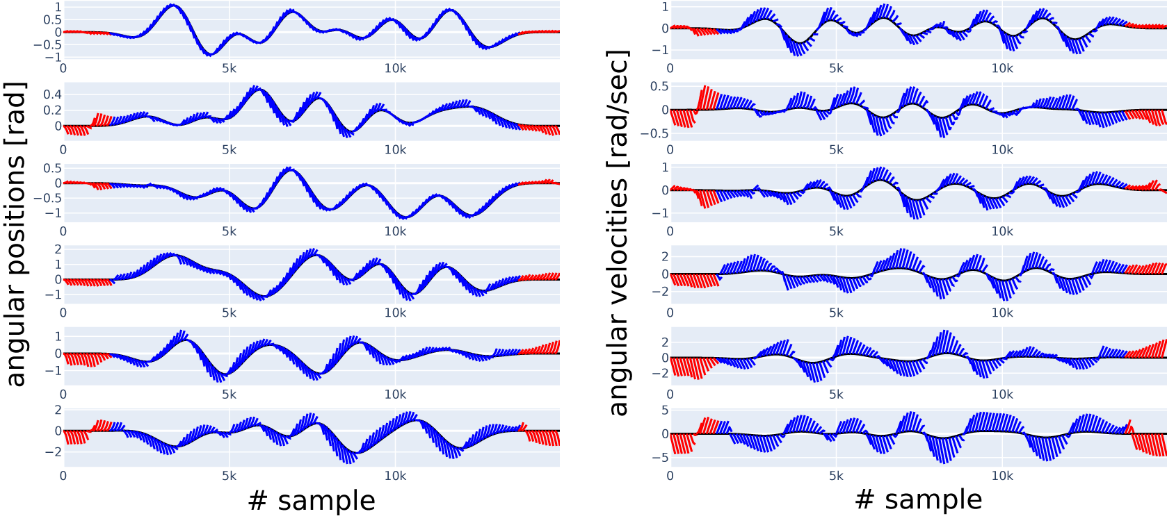
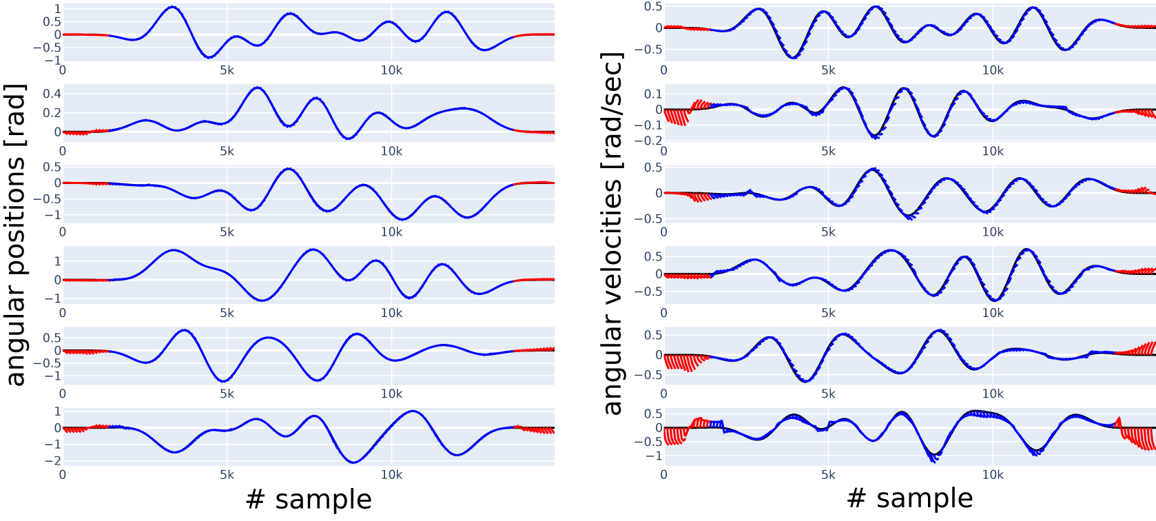
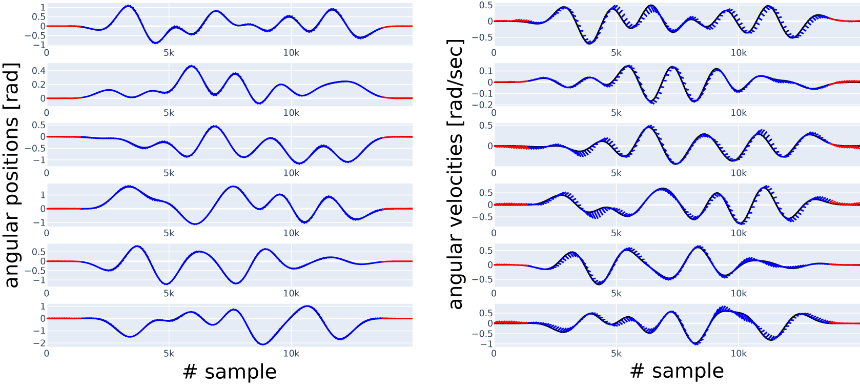
Along with reporting the 150-step-NRMS error as a single number, in Figures 9 and 10, we show some sample simulations (red and blue lines) overlaid with the data (black line), the latter serving as ground truth. Each blue and red line corresponds to a simulation starting from the state at the beginning of the line. The red lines correspond to the regions where the presliding friction can have a substantial effect; all the other lines are shown in blue, corresponding to the region where we expect sliding friction to dominate. Both figures correspond to Case 2 with the reduced datasets, all the blue lines start in this reduced range of the test dataset. Red lines allow us to see the model’s performance outside this range. To be able to distinguish between the lines visually, we show only simulations starting at every 100 samples each, but all the simulations (on the reduced range) are taken into account in the N-step-NRMS error calculation. Lines starting from the same sample number on all the subplots in the same figure belong together as a simulation. An additional figure of this type, Figure 8, shows the simulations of the 0.a initial physics-only model.
Short simulations (indicated in blue and red, with the red part excluded from error calculation in Case 2) versus data (indicated in black), six position (left column) and six velocity (right column) channels, with channel numbers increasing from top to bottom. Result with physics-only Model 0.a, before optimization.
To better compare Model 4 and 0.b, we also show their simulation results overlaid on each other, for two channels, in Figure 11. The red and orange lines correspond to the regions with strong presliding friction. The other lines, in the sliding-dominated range, are shown in green and blue. Orange and green lines correspond to Model 4, while red and blue lines correspond to Model 0.b.
4. Discussion
In this section, we first discuss our best results that belong to Case 2. Afterward, we proceed to Case 1 to add more details about the limitations.
4.1. Case 2: reduced trajectories
In Case 2, we have discarded the regions of strong presliding friction from both the training and the evaluation of the models.
In this case, we observe that the combined Model 4 performs best. Its NRMS error is $ {\eta}_{150}=0.043441 $
, 55% of that of the ANN-only Model 0.b with
$ {\eta}_{150}=0.043441 $
, 55% of that of the ANN-only Model 0.b with $ {\eta}_{150}=0.078613 $
. We consider this a significant difference, which is further reinforced by comparing simulations of these two models in Figure 11. While Figure 11 shows the short simulations in Case 2 for two selected channels, all channels can be inspected for Model 4 in Figure 9, and for Model 0.b in Figure 10. Model 4 is based on the idea that friction depends only on the velocity of the given joint but not on the velocity of the other joints. Another point is that sliding mode friction is often modeled with Coulomb friction, which contains a sign function that is similar to the tanh activation function that we apply in the ANN. We conclude that we have managed to include physical knowledge in the model.
$ {\eta}_{150}=0.078613 $
. We consider this a significant difference, which is further reinforced by comparing simulations of these two models in Figure 11. While Figure 11 shows the short simulations in Case 2 for two selected channels, all channels can be inspected for Model 4 in Figure 9, and for Model 0.b in Figure 10. Model 4 is based on the idea that friction depends only on the velocity of the given joint but not on the velocity of the other joints. Another point is that sliding mode friction is often modeled with Coulomb friction, which contains a sign function that is similar to the tanh activation function that we apply in the ANN. We conclude that we have managed to include physical knowledge in the model.
Short simulations (indicated in blue and red, with the red part excluded from error calculation in Case 2) versus data (indicated in black), six position (left column) and six velocity (right column) channels, with channel numbers increasing from top to bottom. Result in Case 2, Model 4.
Short simulations (indicated in blue and red, with the red part excluded from error calculation in Case 2) versus data (indicated in black), six position (left column) and six velocity (right column) channels, with channel numbers increasing from top to bottom. Result in Case 2, Model 0.b.
Model 5 is the second best with $ {\eta}_{150}=0.064279 $
. While it still performs better than Model 0.b, the difference is insignificant, and it performs notably worse than Model 4. We discarded our hypothesis that the position-dependent load strongly affects the forward dynamics. Different preprocessing of the input positions could also improve the results.
$ {\eta}_{150}=0.064279 $
. While it still performs better than Model 0.b, the difference is insignificant, and it performs notably worse than Model 4. We discarded our hypothesis that the position-dependent load strongly affects the forward dynamics. Different preprocessing of the input positions could also improve the results.
Models 2, 3.a, and 3.b also perform similarly to Model 0.b, and the combined Model 1. performs even worse than Model 0.b. While in these model combinations, we augment the physical model with the ANN in different ways, the real gain is clearly visible when we do so based on information about the structure (i.e., Model 4).
To see how the initial, physics-only model performs, i.e., the one we started from at the beginning of the research, its simulations are available for comparison in Figure 8. We see that the blue and red lines (simulation) are strongly diverging from the black lines (measurement) compared to Figures 9 and 10. The improvement we achieve with other models can mainly be attributed to all containing a universal approximator.
4.2. Case 1: complete trajectories
In Case 1, we use the complete dataset of three trajectories for training, validation, and test, including the regions of strong presliding friction.
In this case, the combined Model 3.b is performing best with $ {\eta}_{150}=0.064798 $
, and Model 2, which has a similar structure to the previously mentioned, is the second best with
$ {\eta}_{150}=0.064798 $
, and Model 2, which has a similar structure to the previously mentioned, is the second best with $ {\eta}_{150}=0.067969 $
. Unfortunately, both are in the same range as the ANN-only Model 0.b which comes third with
$ {\eta}_{150}=0.067969 $
. Unfortunately, both are in the same range as the ANN-only Model 0.b which comes third with $ {\eta}_{150}=0.069210 $
. For this reason, we cannot state that the inclusion of physical information is successful here. We believe the reason is both that our structures are inefficient for the presliding friction, and that the physics-based model does not contain information about it either.
$ {\eta}_{150}=0.069210 $
. For this reason, we cannot state that the inclusion of physical information is successful here. We believe the reason is both that our structures are inefficient for the presliding friction, and that the physics-based model does not contain information about it either.
All the remaining models perform worse than the ANN-only Model 0.b: combining physics-based models with a black-box model does not necessarily improve the results.
5. Conclusions
In this paper, we compared different augmentations of physics-based models with neural networks, using the example of a robot model corresponding to a challenging nonlinear system identification benchmark dataset. The presented model collection equips the users with different exploratory opportunities and gives them additional insight for more educated choices on the model to use to create a more accurate forward dynamics model for the benefit of MPC.
In a general MPC application, we suggest using Model 4, because of its low N-step-NRMS error in Case 2. We have managed to include physical knowledge into this model, as it has a significantly lower error, 55% of that of the ANN-only Model 0.b. A key to achieving this result was selecting the model structure based on insight into the system’s physical structure.
The picture is different if the application targets a region of very low velocities (e.g., very precise positioning). In Case 2, we see that Model 4 improves upon modeling the sliding friction. In contrast, in Case 1, we observe that none of the combined models handle the presliding friction (corresponding to low velocities) particularly well, as neither the physics-based model nor the imposed model structure provides sufficient information about it.
The complexity of the combined models is similar to that of the ANN-only Model 0.b, thus, the noise sensitivity will be approximately the same. On the contrary, compared to Model 0.b, we still managed to improve the generalization capability in Case 2 with Model 4 (Figure 11). Our result reinforces that physics-guided selection of black-box model structures is advantageous, as it has also proven beneficial in other works. For example, in Csurcsia et al. (Reference Csurcsia, Decuyper, Runacres, Renczes and De Troyer2024), the selection of the states included in the nonlinear part of a Polynomial Nonlinear State-Space (PNLSS) model structure is assisted by physical knowledge, in particular the nonlinear distortion levels acquired through frequency domain system identification.
Short simulations versus data. Simulation results of Model 0.b and 4 are overlaid on each other, in Case 2 (red and orange parts are excluded from error calculation in Case 2).

In future research, it would be meaningful to evaluate different ways of preprocessing the features input to the ANN, i.e., applying a transformation to the velocity to emphasize the slight differences. Lowering the computational burden for calculating the robot model within deep learning frameworks would also be a helpful improvement to ensure that the N-step-NRMS error measure (7) can be minimized directly. Furthermore, testing the model’s performance in a real MPC setting would be interesting.
Data availability statement
We worked from a dataset available from Weigand et al. (Reference Weigand, Götz, Ulmen and Ruskowski2022). The code corresponding to this research is available on GitHub under https://github.com/ha7ilm/roblue, commit 9dd1dcb at the time of writing.
Acknowledgments
We thank the team that prepared the open-source robot dataset for Weigand et al. (Reference Weigand, Götz, Ulmen and Ruskowski2022).
Author contribution
-
• Conceptualization: András Retzler, Maarten Schoukens
-
• Methodology: András Retzler, Roland Tóth, Gerben Beintema, Jean-Philippe Noël, Maarten Schoukens, Jonas Weigand, Zsolt Kollár, Jan Swevers
-
• Software: András Retzler, Gerben Beintema
-
• Writing—Original Draft: András Retzler
-
• Data Curation: Jonas Weigand
-
• Supervision: Jan Swevers, Zsolt Kollár
All authors approved the final submitted draft.
Funding statement
This research was partially supported by Flanders Make: SBO project DIRAC: Deterministic and Inexpensive Realizations of Advanced Control, and ICON project ID2CON: Integrated IDentification for CONtrol, and by the Research Foundation - Flanders (FWO - Flanders) through project G0A6917N. The research reported in this paper was partially carried out at the Budapest University of Technology and Economics, and it has been supported by the National Research, Development, and Innovation Fund of Hungary under Grant TKP2021-EGA-02, and the János Bólyai Research Grant (BO/0042/23/6) of the Hungarian Academy of Sciences.
Competing interest
The authors declare none.
Ethical standard
The research meets all ethical guidelines, including adherence to the legal requirements of the study country. To adhere to the publisher’s ethical guidelines on “AI Contribution to Research Content,” it is acknowledged that OpenAI Codex, GPT-3.5, and GPT-4 models were used (versions up to January 24, 2024) to help in the activities related to writing and editing the text and formulas of this paper and the corresponding software source code, but the authors have checked to the best of their ability the correctness of any output generated with AI.


 Open access
Comments
No Comments have been published for this article.