


Impact Statement
Nonintrusive model order reduction (MOR) technique that can reduce models of generalized forms is desired in many industrial fields. Among available methods, MOR combined with artificial neural network (ANN) has great potential. However, most of the current ANN-based MOR methods ignore the fact that the target system is actually evaluated by an unknown numerical solver. Runge–Kutta neural network (RKNN) is a type of ANN that treats the time-series data as a result of numerical integration. This concept also makes RKNN more physics-informed, which can be a novel basis for further research. Therefore, investigating the capability of using this architecture for learning in the reduced space is meaningful.
1. Introduction
Physics-based simulation has been an integral part of product development and design as a cheaper alternative to physical prototyping. On the one hand, large computational resource enables using complex simulation models in the design phase. On the other hand, small form-factor hardware is also readily available, enabling “edge computing,” that is deploying compact computing devices in factories and smart buildings to enable data analysis. The existence of such hardware opens up the possibility of transferring the physics-based models from design phase into the operation phase. This is a key part of the digital twin vision (Hartmann et al., Reference Hartmann, Herz and Wever2018; Rasheed et al., Reference Rasheed, San and Kvamsdal2019). A digital twin running next to the device can enable novel industrial solutions such as model-based predictive maintenance or model-based process optimization.
However, bringing highly complex simulation models into the operation phase presents several challenges which are not present in the design phase. Firstly, the memory footprint of such models needs to be reduced to fit within the limited memory of edge devices, alongside the rest of the other potential data-analysis processes. Secondly, the models need to run at or faster than real-time on the limited hardware of edge devices. The methods which transform simulation models to comply with such requirements are known under the umbrella term of model order reduction (MOR; Antoulas, Reference Antoulas2005; Hinze and Volkwein, Reference Hinze and Volkwein2005; Willcox and Peraire, Reference Willcox and Peraire2002).
Most MOR techniques rely on mapping the high-dimensional state of the full order model (FOM) into a lower-dimensional space where the reduced order model (ROM) is to be solved. Within this contribution, we look into proper orthogonal decomposition (POD), one of the most widely used methods for finding such mapping (Willcox and Peraire, Reference Willcox and Peraire2002; Hinze and Volkwein, Reference Hinze and Volkwein2005). POD is based on performing principal component analysis (PCA) on model trajectories generated by the original FOM, known as snapshots.
For linear models, knowing the dimension-reduction mapping and the equations which define the FOM is enough to obtain an ROM through projection. However, this cannot be done for complex models with nonlinearities. In this case, a model-reconstruction step is needed in order to reproduce the nonlinear behaviors in the reduced space. There are several methods perform this step, such as discrete empirical interpolation (Chaturantabut and Sorensen, Reference Chaturantabut and Sorensen2010), operator inference (Peherstorfer and Willcox, Reference Peherstorfer and Willcox2016), and long-short-term-memory neural network (NN)s (Mohan and Gaitonde, Reference Mohan and Gaitonde2018). Besides, recurrent NNs (Kosmatopoulos et al., Reference Kosmatopoulos, Polycarpou, Christodoulou and Ioannou1995), have also been used for this purpose (Kani and Elsheikh, Reference Kani and Elsheikh2017; Wang et al., Reference Wang, Ripamonti and Hesthaven2020). As a universal approximator, a standard multilayer perceptron (MLP) NN also can be used for this purpose. Sometimes, ROMs which are flexible with the time-stepping are required. In this case, networks such as RS-ResNet (Qin et al., Reference Qin, Wu and Xiu2019) can be employed. However, a disadvantage of this kind of networks is the requirement of training different networks for different time steps. Therefore, the flexibility is restricted by the number of the trained networks. Apart from these, we also would like to point out the numerical-integration-based NN models such as explicit Euler NN (EENN; (Pan and Duraisamy, Reference Pan and Duraisamy2018) and Runge–Kutta NN (RKNN; Wang and Lin, Reference Wang and Lin1998) specialize in nonintrusively modeling the solution of ordinary differential equation (ODE) or partial differential equation (PDE). Moreover, these networks can efficiently learn the time information in the training data and be more flexible to the time stepping strategy. Therefore, their potential of reconstructing the ROMs is worth investigation.
The combination of POD for dimension reduction and machine learning represents a purely-data-driven MOR frameworkfor the complex problems (Agudelo et al., 2009; Ubbiali, 2017; Pawar et al., 2019). The main contribution of this work consists in exploring methodological variations to this framework. On the one hand, the effects of different approaches to generate the snapshot data for POD are investigated. On the other hand, the impact of using different NN architectures is explored. Although by some means the intrusive methods can be applied to reduce the test models investigated in this work, we will consider in a more generalized scope where we have very limited access to the FOM solver and a nonintrusive solution is necessary. Therefore, conventional intrusive methods are not studied in this work.
The paper is organized as follows. The introduction to POD and the modification for taking snapshots of the FOMs is given in Section 2. The principles and architectures of different networks are described in Section 3, numerical experiment evaluating the proposed MOR framework are given in Section 4, and their results are shown in Section 5. Finally, the conclusions follow in Section 6.
2. Proper Orthogonal Decomposition
In the last decades, there have been many efforts to develop different techniques in order to obtain compact low-dimensional representations of high-dimensional datasets. These representations, in general, encapsulate the most important information while discarding less important components. Some applications include image compression using PCA (Du and Fowler, Reference Du and Fowler2007), data visualization using t-SNE (van der Maaten and Hinton, Reference van der Maaten and Hinton2008) and structural description of data using diffusion maps (Coifman et al., Reference Coifman, Lafon, Lee, Maggioni, Nadler, Warner and Zucker2005). Here, the focus will be on POD, which is a variant of PCA in the field of MOR.
POD can find a reduced basis $ \boldsymbol{V} $
of arbitrary dimension that optimally represents (in a least square sense) the trajectories of the FOM used as snapshots. This basis can be used to project such snapshots into the low-dimensional space.
$ \boldsymbol{V} $
of arbitrary dimension that optimally represents (in a least square sense) the trajectories of the FOM used as snapshots. This basis can be used to project such snapshots into the low-dimensional space.
2.1. Problem statement
The full-dimensional problem that we intend to reduce in this work is an ordinary differential equation (ODE) typically originating from a spatial discretization from a multidimensional PDE. This ODE is frequently used as the governing equation for many engineering problems. The equation can be written as:
 $$ \dot{\boldsymbol{y}}(t)=\boldsymbol{f}\left(\boldsymbol{y}(t);\boldsymbol{\mu} (t)\right), $$
where $ \boldsymbol{y}\ \in\ {R}^N $
is the state vector of the FOM,
$ \boldsymbol{y}\ \in\ {R}^N $
is the state vector of the FOM, $ t\ \in\ \left[{t}_0,{t}_{\mathrm{end}}\right] $
is the time, and
$ t\ \in\ \left[{t}_0,{t}_{\mathrm{end}}\right] $
is the time, and $ \mu\ \in\ {R}^{n_{\mu }} $
is the vector of the system parameters.
$ \mu\ \in\ {R}^{n_{\mu }} $
is the vector of the system parameters. $ N $
is the number of variables in state vector will be called the size of the FOM and
$ N $
is the number of variables in state vector will be called the size of the FOM and $ {n}_{\mu } $
is the number of system parameters. The target of MOR is to find a reduced model, with size
$ {n}_{\mu } $
is the number of system parameters. The target of MOR is to find a reduced model, with size $ {N}_r\hskip1.5pt \ll \hskip1.5pt N $
, which can reproduce the solution of the FOM to a certain accuracy for a given set of system parameters
$ {N}_r\hskip1.5pt \ll \hskip1.5pt N $
, which can reproduce the solution of the FOM to a certain accuracy for a given set of system parameters $ \boldsymbol{\mu} (t) $
. This goal will be achieved by mapping the FOM into a reduced space with the help of a reduced basis
$ \boldsymbol{\mu} (t) $
. This goal will be achieved by mapping the FOM into a reduced space with the help of a reduced basis $ \boldsymbol{V} $
. As briefly described before, the reduced basis is constructed from the snapshots of the FOM. Snapshots are nothing but a set of solutions,
$ \boldsymbol{V} $
. As briefly described before, the reduced basis is constructed from the snapshots of the FOM. Snapshots are nothing but a set of solutions, $ \Big\{{\boldsymbol{y}}_{\mathbf{1}},{\boldsymbol{y}}_{\mathbf{2}},\dots, $ $ {\boldsymbol{y}}_{{\boldsymbol{N}}_{\boldsymbol{s}}}\Big\} $
, to the FOM Equation (1) with corresponding system parameter configurations
$ {\boldsymbol{y}}_{{\boldsymbol{N}}_{\boldsymbol{s}}}\Big\} $
, to the FOM Equation (1) with corresponding system parameter configurations $ \left\{{\boldsymbol{\mu}}_{\mathbf{1}},{\boldsymbol{\mu}}_{\mathbf{2}},\dots, {\boldsymbol{\mu}}_{\boldsymbol{Ns}}\right\} $
. Here,
$ \left\{{\boldsymbol{\mu}}_{\mathbf{1}},{\boldsymbol{\mu}}_{\mathbf{2}},\dots, {\boldsymbol{\mu}}_{\boldsymbol{Ns}}\right\} $
. Here, $ {N}_s $
is the number of snapshots taken for the FOM. Often, these snapshots will present in the form of matrix called snapshot matrix
$ {N}_s $
is the number of snapshots taken for the FOM. Often, these snapshots will present in the form of matrix called snapshot matrix $ \boldsymbol{Y}=\left[{\boldsymbol{y}}_{\mathbf{1}},{\boldsymbol{y}}_{\mathbf{2}},\dots, {\boldsymbol{y}}_{{\boldsymbol{N}}_{\boldsymbol{s}}}\right]\ \in\ {R}^{N\times \left({N}_s\cdot k\right)} $
, where
$ \boldsymbol{Y}=\left[{\boldsymbol{y}}_{\mathbf{1}},{\boldsymbol{y}}_{\mathbf{2}},\dots, {\boldsymbol{y}}_{{\boldsymbol{N}}_{\boldsymbol{s}}}\right]\ \in\ {R}^{N\times \left({N}_s\cdot k\right)} $
, where $ k $
is the number of time steps in each simulation.
$ k $
is the number of time steps in each simulation.
2.2. Taking snapshots: static-parameter sampling (SPS) and dynamic-parameter sampling (DPS)
Since the reduced basis $ \boldsymbol{V} $
is constructed based on the snapshot matrix
$ \boldsymbol{V} $
is constructed based on the snapshot matrix $ \boldsymbol{Y} $
and later the snapshot will also be used to train the artificial NN (ANN), the quality of the snapshots is crucial to the performance of the whole framework. Here, in this paper, we propose a new sampling strategy, DPS, for taking snapshots to capture the dynamics of the FOM as much as possible.
$ \boldsymbol{Y} $
and later the snapshot will also be used to train the artificial NN (ANN), the quality of the snapshots is crucial to the performance of the whole framework. Here, in this paper, we propose a new sampling strategy, DPS, for taking snapshots to capture the dynamics of the FOM as much as possible.
The conventional way to define the system parameters $ \boldsymbol{\mu} $
during each snapshot simulation is to choose constant values
$ \boldsymbol{\mu} $
during each snapshot simulation is to choose constant values $ \boldsymbol{\mu} (\boldsymbol{t})=\boldsymbol{\mu} ({\boldsymbol{t}}_{\mathbf{0}}) $
using some sparse sampling technique such as Sparse Grids, Latin Hypercube Sampling (Helton and Davis, Reference Helton and Davis2003), Hammersley Sampling, and Halton Sampling (Wong et al., Reference Wong, Luk and Heng1997). Some strategies can select those constant parameter values smartly, among which the greedy sampling (Bui-Thanh, Reference Bui-Thanh2007; Haasdonk et al., Reference Haasdonk, Dihlmann and Ohlberger2011; Lappano et al., Reference Lappano, Naets, Desmet, Mundo and Nijman2016) is probably the most well-known. Although greedy sampling techniques have been proven highly successful for projection-based, intrusive MOR methods, they are difficult to apply to the reduction methods used in this work. This is because we do not count with a priori error estimator and a posteriori error calculation would require the retraining of the NNs during the evaluation of the snapshots, which is unfeasible due to computational costs. Therefore, DPS is proposed in this work as the alternative snapshot collection strategy for non-intrusive MOR.
$ \boldsymbol{\mu} (\boldsymbol{t})=\boldsymbol{\mu} ({\boldsymbol{t}}_{\mathbf{0}}) $
using some sparse sampling technique such as Sparse Grids, Latin Hypercube Sampling (Helton and Davis, Reference Helton and Davis2003), Hammersley Sampling, and Halton Sampling (Wong et al., Reference Wong, Luk and Heng1997). Some strategies can select those constant parameter values smartly, among which the greedy sampling (Bui-Thanh, Reference Bui-Thanh2007; Haasdonk et al., Reference Haasdonk, Dihlmann and Ohlberger2011; Lappano et al., Reference Lappano, Naets, Desmet, Mundo and Nijman2016) is probably the most well-known. Although greedy sampling techniques have been proven highly successful for projection-based, intrusive MOR methods, they are difficult to apply to the reduction methods used in this work. This is because we do not count with a priori error estimator and a posteriori error calculation would require the retraining of the NNs during the evaluation of the snapshots, which is unfeasible due to computational costs. Therefore, DPS is proposed in this work as the alternative snapshot collection strategy for non-intrusive MOR.
DPS, just as its name implies, we use time-dependent parameter values to construct the ith snapshot solution $ {\boldsymbol{y}}_i $
so that it satisfies
$ {\boldsymbol{y}}_i $
so that it satisfies
 $$ {\dot{\boldsymbol{y}}}_i=\boldsymbol{f}\left({\boldsymbol{y}}_i;{\boldsymbol{\mu}}_{\boldsymbol{i}}(t)\right). $$
We would like to select the values for the $ {\boldsymbol{\mu}}_{\boldsymbol{i}} $
from a function space
$ {\boldsymbol{\mu}}_{\boldsymbol{i}} $
from a function space
 $$ \mathcal{F}=\left\{\mu :\left[{t}_0,{t}_{\mathrm{end}}\right]\to \Omega \right\}, $$
where $ \left[{t}_0,{t}_{\mathrm{end}}\right]\subset R $
is the time span and
$ \left[{t}_0,{t}_{\mathrm{end}}\right]\subset R $
is the time span and $ \Omega =\left[{\mu}_1^{min},{\mu}_1^{max}\right]\times \left[{\mu}_2^{min},{\mu}_2^{max}\right]\times \dots \times \left[{\mu}_{n_{\mu}}^{min},{\mu}_{n_{\mu}}^{max}\right] $
is a hypercube defined by the limits of the individual components of the the parameter vector. In principle, we could use any finite subset of
$ \Omega =\left[{\mu}_1^{min},{\mu}_1^{max}\right]\times \left[{\mu}_2^{min},{\mu}_2^{max}\right]\times \dots \times \left[{\mu}_{n_{\mu}}^{min},{\mu}_{n_{\mu}}^{max}\right] $
is a hypercube defined by the limits of the individual components of the the parameter vector. In principle, we could use any finite subset of $ \mathcal{F} $
to build our snapshots. In this work, we decided to use sinusoidal function for dynamic sampling as an example. These functions are constructed as follows:
$ \mathcal{F} $
to build our snapshots. In this work, we decided to use sinusoidal function for dynamic sampling as an example. These functions are constructed as follows:
-
1. Use any multivariate sampling, for example, Hammersley sequence is used in this work, to select $ {N}_s $
parameter vectors
$ \left\{{\boldsymbol{\mu}}_{\mathbf{1}},{\boldsymbol{\mu}}_{\mathbf{2}},\dots, {\boldsymbol{\mu}}_{{\boldsymbol{N}}_{\boldsymbol{s}}}\right\} $
.
$ {N}_s $
parameter vectors
$ \left\{{\boldsymbol{\mu}}_{\mathbf{1}},{\boldsymbol{\mu}}_{\mathbf{2}},\dots, {\boldsymbol{\mu}}_{{\boldsymbol{N}}_{\boldsymbol{s}}}\right\} $
. -
2. Select
$ {N}_s $
randomly distributed values for the angular frequency
$ \left\{{\omega}_1,\dots, {\omega}_{N_s}\right\}\subset \left[0,{\omega}_{max}\right] $
, where
$ {\omega}_{max}=4 $
, selected so that the functions have a maximum of 4 oscillations within the time frame. -
3. Define the parameter functions as
(4)where
$ {\boldsymbol{\mu}}_i^{amp}={\boldsymbol{\mu}}_{\boldsymbol{i}}-{\boldsymbol{\mu}}_{min} $
and
$ {\boldsymbol{\mu}}_{min}=\left[{\mu}_1^{min},{\mu}_2^{min},\dots, {\mu}_{n_{\mu}}^{min}\right] $
.


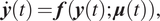
A graphical representation of representative function is shown in Figure 1.
An example showing the relation and difference between static-parameter sampling (SPS) and dynamic-parameter sampling (DPS). We assume the parameter space is designed as $ \left[\mathrm{0,100}\right]\times \left[\mathrm{0,100}\right] $
. Orange: the parameter configuration
$ \left[\mathrm{0,100}\right]\times \left[\mathrm{0,100}\right] $
. Orange: the parameter configuration $ \boldsymbol{\mu} =\left[80,40\right] $
is selected for running one snapshot simulation. Blue: the parameter configuration
$ \boldsymbol{\mu} =\left[80,40\right] $
is selected for running one snapshot simulation. Blue: the parameter configuration $ \boldsymbol{\mu} (t)=\left[80|\mathit{\sin}\left(4\pi /100t\right)|,40|\mathit{\sin}\left(4\pi /100t\right)|\right] $
is selected for running one snapshot simulation.
$ \boldsymbol{\mu} (t)=\left[80|\mathit{\sin}\left(4\pi /100t\right)|,40|\mathit{\sin}\left(4\pi /100t\right)|\right] $
is selected for running one snapshot simulation.
The solutions of Equation (2) using parameters defined by Equation (4) are the snapshots we use for DPS. The snapshots contain the dynamic response of the system with certain parameter configurations. And more dynamic modes are included in the snapshots, more essential information about the system is available to the reduction. Moreover, since the input–output response of the system will be fed into the NN in Section 3, the diversity of the snapshots will strongly influence the training procedure. In this aspect, DPS can provide us with more diverse observation to the system’s response.
We must clarify that the procedure used to define the input parameters functions is arbitrary. The sinusoidal range and frequency of the sinusoidal function should: (a) cover the whole relevant value range of the parameters and (b) incorporate time dependent effects. The limit in the maximum frequency chosen relatively small because of the nature of the problems used as test cases. It is possible to consider the use of other functions instead of sinusoidal functions. As an example, Qin et al. (Reference Qin, Chen, Jakeman and Xiu2021) have defined time-dependent input functions using low-order polynomials. We favor sinusoidal functions, because we can more easily ensure that their values fall within the limits we define for the individual parameters. We defer the exploration of alternatives to future research.
2.3. Singular value decomposition
With the snapshots obtained in the Section 2.2, the goal is to find an appropriate reduced basis $ {\left\{{\boldsymbol{v}}_{\boldsymbol{i}}\right\}}_{i=1}^{N_r} $
which minimizes the approximation error (Chaturantabut and Sorensen, Reference Chaturantabut and Sorensen2010):
$ {\left\{{\boldsymbol{v}}_{\boldsymbol{i}}\right\}}_{i=1}^{N_r} $
which minimizes the approximation error (Chaturantabut and Sorensen, Reference Chaturantabut and Sorensen2010):
where $ {\boldsymbol{y}}_{\boldsymbol{i}} $
stands for
$ {\boldsymbol{y}}_{\boldsymbol{i}} $
stands for $ \boldsymbol{y}\left({\boldsymbol{\mu}}_{\boldsymbol{i}}\right) $
.
$ \boldsymbol{y}\left({\boldsymbol{\mu}}_{\boldsymbol{i}}\right) $
.
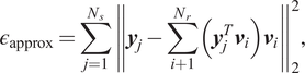
The minimization of $ {\varepsilon}_{\mathrm{approx}} $
in Equation (5) can be solved by singular value decomposition of the snapshot matrix
$ {\varepsilon}_{\mathrm{approx}} $
in Equation (5) can be solved by singular value decomposition of the snapshot matrix $ \boldsymbol{Y}=\left[{\boldsymbol{y}}_{\mathbf{1}},{\boldsymbol{y}}_{\mathbf{2}},\dots, {\boldsymbol{y}}_{{\boldsymbol{N}}_{\boldsymbol{s}}}\right]\in {R}^{N\times \left({N}_s\cdot k\right)} $
:
$ \boldsymbol{Y}=\left[{\boldsymbol{y}}_{\mathbf{1}},{\boldsymbol{y}}_{\mathbf{2}},\dots, {\boldsymbol{y}}_{{\boldsymbol{N}}_{\boldsymbol{s}}}\right]\in {R}^{N\times \left({N}_s\cdot k\right)} $
:
 $$ \boldsymbol{Y}=\boldsymbol{V}\varSigma {\boldsymbol{W}}^T. $$
If the rank of the matrix $ \boldsymbol{Y} $
is
$ \boldsymbol{Y} $
is $ k $
, then the matrix
$ k $
, then the matrix $ \boldsymbol{V}\in {R}^{N\times k} $
consists of
$ \boldsymbol{V}\in {R}^{N\times k} $
consists of $ k $
column vectors
$ k $
column vectors $ \left\{{\boldsymbol{v}}_i, i=1,2,\dots, k\right\} $
, and matrix
$ \left\{{\boldsymbol{v}}_i, i=1,2,\dots, k\right\} $
, and matrix $ \boldsymbol{\Sigma} $
is a diagonal matrix
$ \boldsymbol{\Sigma} $
is a diagonal matrix $ \mathit{\operatorname{diag}}\left({\sigma}_1,{\sigma}_2,\dots, {\sigma}_k\right) $
.
$ \mathit{\operatorname{diag}}\left({\sigma}_1,{\sigma}_2,\dots, {\sigma}_k\right) $
. $ {\sigma}_i $
is called ith singular value corresponding to ith singular vector
$ {\sigma}_i $
is called ith singular value corresponding to ith singular vector $ {\boldsymbol{v}}_{\boldsymbol{i}} $
.
$ {\boldsymbol{v}}_{\boldsymbol{i}} $
.
Essentially, each singular vector $ {\boldsymbol{v}}_i $
represents a dynamic mode of the system. And the corresponding singular value
$ {\boldsymbol{v}}_i $
represents a dynamic mode of the system. And the corresponding singular value $ {\sigma}_i $
of singular vector
$ {\sigma}_i $
of singular vector $ {\boldsymbol{v}}_i $
can be seen as the “weight” of the dynamic mode
$ {\boldsymbol{v}}_i $
can be seen as the “weight” of the dynamic mode $ {\boldsymbol{v}}_i $
. Since the greater the weight, the more important the dynamic mode is,
$ {\boldsymbol{v}}_i $
. Since the greater the weight, the more important the dynamic mode is, $ {N}_r $
singular vectors corresponding to the greatest
$ {N}_r $
singular vectors corresponding to the greatest $ {N}_r $
singular values will be used to construct the reduced basis
$ {N}_r $
singular values will be used to construct the reduced basis $ {\boldsymbol{V}}_r=\left[{\boldsymbol{v}}_1,{\boldsymbol{v}}_2,\dots, {\boldsymbol{v}}_{N_r}\right]\in {R}^{N\times {N}_r} $
. Theoretically, the reduced model will have better quality if more dynamic modes are retained in
$ {\boldsymbol{V}}_r=\left[{\boldsymbol{v}}_1,{\boldsymbol{v}}_2,\dots, {\boldsymbol{v}}_{N_r}\right]\in {R}^{N\times {N}_r} $
. Theoretically, the reduced model will have better quality if more dynamic modes are retained in $ \boldsymbol{V} $
, but this will also increase the size of the reduced model. And since some high frequency noise with small singular value might also be observed in snapshots and later included in the reduced model, the reduced dimension must be selected carefully. For research regarding this topic, we refer to Josse and Husson (Reference Josse and Husson2012) and Valle et al. (Reference Valle, Li and Qin1999), and we will not further study it in this work.
$ \boldsymbol{V} $
, but this will also increase the size of the reduced model. And since some high frequency noise with small singular value might also be observed in snapshots and later included in the reduced model, the reduced dimension must be selected carefully. For research regarding this topic, we refer to Josse and Husson (Reference Josse and Husson2012) and Valle et al. (Reference Valle, Li and Qin1999), and we will not further study it in this work.
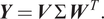
The high-dimensional Equation (1) can be projected into the reduced space using the reduced basis:
 $$ {\boldsymbol{V}}^T\boldsymbol{V}{\dot{\boldsymbol{y}}}_{\boldsymbol{r}}(t)={\boldsymbol{V}}^T\boldsymbol{f}\left({\boldsymbol{V}\boldsymbol{y}}_{\boldsymbol{r}};\boldsymbol{\mu} \right), $$
where $ {\boldsymbol{y}}_{\boldsymbol{r}} $
is the reduced state vector. And if the orthonormality of the column vectors in
$ {\boldsymbol{y}}_{\boldsymbol{r}} $
is the reduced state vector. And if the orthonormality of the column vectors in $ \boldsymbol{V} $
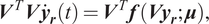
is considered, the Equation (7) can be simplified to:
$ \boldsymbol{V} $
is considered, the Equation (7) can be simplified to:
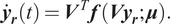 $$ {\dot{\boldsymbol{y}}}_{\boldsymbol{r}}(t)={\boldsymbol{V}}^T\boldsymbol{f}\left({\boldsymbol{V}\boldsymbol{y}}_{\boldsymbol{r}};\boldsymbol{\mu} \right). $$
In Equation (8), if $ \boldsymbol{f}\left(\cdot \right) $
is a linear function of
$ \boldsymbol{f}\left(\cdot \right) $
is a linear function of $ \boldsymbol{y} \approx \hskip0.15em {\boldsymbol{Vy}}_{\boldsymbol{r}} $
, then further reduction can be applied and leads to:
$ \boldsymbol{y} \approx \hskip0.15em {\boldsymbol{Vy}}_{\boldsymbol{r}} $
, then further reduction can be applied and leads to:
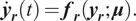 $$ {\dot{\boldsymbol{y}}}_{\boldsymbol{r}}(t)={\boldsymbol{f}}_{\boldsymbol{r}}\left({\boldsymbol{y}}_{\boldsymbol{r}};\boldsymbol{\mu} \right). $$
However, if we consider a more generalized form of $ \boldsymbol{f}\left(\cdot \right) $
, that is the function can be either linear or nonlinear to
$ \boldsymbol{f}\left(\cdot \right) $
, that is the function can be either linear or nonlinear to $ \boldsymbol{y} $
, the evaluation of
$ \boldsymbol{y} $
, the evaluation of $ \boldsymbol{f}\left(\cdot \right) $
still requires lifting
$ \boldsymbol{f}\left(\cdot \right) $
still requires lifting $ {\boldsymbol{y}}_{\boldsymbol{r}} $
to
$ {\boldsymbol{y}}_{\boldsymbol{r}} $
to $ {\boldsymbol{Vy}}_{\boldsymbol{r}} $
. This lifting and evaluation is performed during the online phase and can significantly reduce the efficiency of the ROM. A solution to this problem can be using an approximator (e.g., NN) to construct a new function satisfying
$ {\boldsymbol{Vy}}_{\boldsymbol{r}} $
. This lifting and evaluation is performed during the online phase and can significantly reduce the efficiency of the ROM. A solution to this problem can be using an approximator (e.g., NN) to construct a new function satisfying $ \hat{\boldsymbol{f}}\left({\boldsymbol{y}}_{\boldsymbol{r}};\boldsymbol{\mu} \right)\hskip0.15em \approx \hskip0.15em {\boldsymbol{V}}^T\boldsymbol{f}\left({\boldsymbol{V}\boldsymbol{y}}_{\boldsymbol{r}};\boldsymbol{\mu} \right) $
.
$ \hat{\boldsymbol{f}}\left({\boldsymbol{y}}_{\boldsymbol{r}};\boldsymbol{\mu} \right)\hskip0.15em \approx \hskip0.15em {\boldsymbol{V}}^T\boldsymbol{f}\left({\boldsymbol{V}\boldsymbol{y}}_{\boldsymbol{r}};\boldsymbol{\mu} \right) $
.
3. Prediction by NN
After finding the projection into the lower-dimensional space, we need a way to reproduce the projected dynamics which is governed by Equation (1) in the full-order space. In this work, we consider three NN architectures: MLP, EENN, and RKNN.
In all cases the training data uses the snapshots projected into the reduced space.
 $$ {\displaystyle \begin{array}{ll}{\boldsymbol{Y}}_r& ={\boldsymbol{V}}^{\boldsymbol{T}}\boldsymbol{Y}\\ {}& ={\boldsymbol{V}}^{\boldsymbol{T}}\left[{\mathbf{y}}_1,{\mathbf{y}}_2,\dots, {\mathbf{y}}_{N_s}\right]\\ {}& =\left[{\mathbf{y}}_{r,1},{\mathbf{y}}_{r,2},\dots, {\mathbf{y}}_{r,{N}_s}\right],\end{array}} $$
where
 $$ {\mathbf{y}}_{r, i}=\left[{\mathbf{y}}_{r, i}\left({t}_1\right),\dots, {\mathbf{y}}_{r, i}\left({t}_k\right)\right] $$
is the projected trajectories corresponding to the parameter $ {\mu}_i(t) $
and
$ {\mu}_i(t) $
and $ k $
is the number of time steps used for each snapshot simulation. If we denote the step size with
$ k $
is the number of time steps used for each snapshot simulation. If we denote the step size with $ \tau $
, we will have
$ \tau $
, we will have
We also note that $ {\mathbf{Y}}_r\in {\mathrm{\mathbb{R}}}^{N_r\times \left({N}_s\cdot k\right)} $
.
$ {\mathbf{Y}}_r\in {\mathrm{\mathbb{R}}}^{N_r\times \left({N}_s\cdot k\right)} $
.
All the types of networks in this paper use the rectified linear unit (Glorot et al., Reference Glorot, Bordes and Bengio2011) as the activation functions for enhancing the capability to approximating generalized nonlinearity. For updating the parameters of the networks, the backpropagation (Rumelhart et al., Reference Rumelhart, Hinton and Williams1986) is the method applied in this work. For doing this, the Adam optimizer (Kingma and Ba, Reference Kingma and Ba2014) is used and L2 regularization is deployed to prevent overfitting.
3.1. Multilayer perceptron
If the time step in the training data is the same as the desired time step in validation, the most straightforward strategy of predicting the state in the future is to map all current information, that is state vector and input parameters, to the future state vector. This is exactly how MLP network learns to predict the evolution of the system. Its concept of learning the relation between each pair of neighboring state vectors is shown in Figure 2.
Picture of the structure of multilayer perceptron (MLP). MLPs approximate the new state $ {\boldsymbol{y}}_{r,i}\left({t}_{j+1}\right) $
based on the given input
$ {\boldsymbol{y}}_{r,i}\left({t}_{j+1}\right) $
based on the given input $ {\boldsymbol{y}}_{r,i}\left({t}_j\right) $
and
$ {\boldsymbol{y}}_{r,i}\left({t}_j\right) $
and $ \boldsymbol{\mu} \left({t}_j\right) $
.
$ \boldsymbol{\mu} \left({t}_j\right) $
.
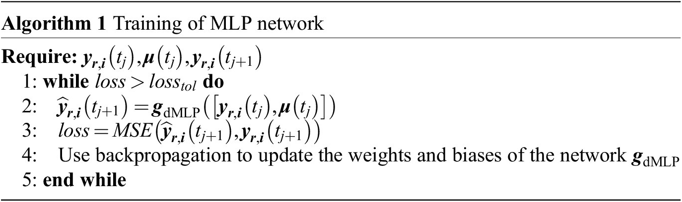
In Algorithm 1, $ {\boldsymbol{y}}_{\boldsymbol{r},\boldsymbol{i}}\left({t}_j\right) $
and
$ {\boldsymbol{y}}_{\boldsymbol{r},\boldsymbol{i}}\left({t}_j\right) $
and
![]() are the state vectors stored in the snapshots, and
are the state vectors stored in the snapshots, and $ \boldsymbol{\mu} \left({t}_j\right) $
is the parameter vector at the corresponding time instance. The operation
$ \boldsymbol{\mu} \left({t}_j\right) $
is the parameter vector at the corresponding time instance. The operation $ \left[ A, B\right] $
means to concatenate two arrays. Without loss of generality, we assume both
$ \left[ A, B\right] $
means to concatenate two arrays. Without loss of generality, we assume both $ {\boldsymbol{y}}_{\boldsymbol{r},\boldsymbol{i}}\left({t}_j\right) $
and
$ {\boldsymbol{y}}_{\boldsymbol{r},\boldsymbol{i}}\left({t}_j\right) $
and $ \boldsymbol{\mu} \left({t}_j\right) $
are column vectors, then this operation will vertically stack them in sequence. The loss function used in this paper is mean-square error (MSE), it computes the error between the approximation and the target by:
$ \boldsymbol{\mu} \left({t}_j\right) $
are column vectors, then this operation will vertically stack them in sequence. The loss function used in this paper is mean-square error (MSE), it computes the error between the approximation and the target by:
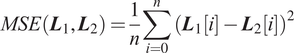 $$ MSE\left({\boldsymbol{L}}_1,{\boldsymbol{L}}_2\right)=\frac{1}{n}\sum \limits_{i=0}^n{\left({\boldsymbol{L}}_1\left[ i\right]-{\boldsymbol{L}}_2\left[ i\right]\right)}^2 $$
here $ n $
is the number of elements in both arrays, and
$ n $
is the number of elements in both arrays, and $ i $
in the square brackets means ith element of the array. The same notation and loss function is also used for the networks introduced in the next sections.
$ i $
in the square brackets means ith element of the array. The same notation and loss function is also used for the networks introduced in the next sections.
3.2. Explicit Euler neural network
As an alternative to learning the mapping between states of two consecutive time steps, it is possible to learn the approximation $ \hat{\boldsymbol{f}}\left(\cdot \right) $
to the R.H.S. of the reduced governing equations (Equation (8)). In this case, the inputs to the NN are again the current state of the system
$ \hat{\boldsymbol{f}}\left(\cdot \right) $
to the R.H.S. of the reduced governing equations (Equation (8)). In this case, the inputs to the NN are again the current state of the system $ {\boldsymbol{y}}_{\boldsymbol{r},\boldsymbol{i}}\left({t}_j\right) $
and
$ {\boldsymbol{y}}_{\boldsymbol{r},\boldsymbol{i}}\left({t}_j\right) $
and $ \boldsymbol{\mu} ({\boldsymbol{y}}_{\boldsymbol{j}}) $
, but the new state is now calculated as
$ \boldsymbol{\mu} ({\boldsymbol{y}}_{\boldsymbol{j}}) $
, but the new state is now calculated as
where $ {\boldsymbol{g}}_{\mathrm{eeMLP}}\left({t}_j,\mu \right) $
is an MLP used as the approximator to the R.H.S.
$ {\boldsymbol{g}}_{\mathrm{eeMLP}}\left({t}_j,\mu \right) $
is an MLP used as the approximator to the R.H.S.
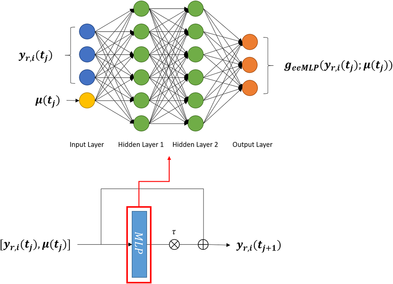
We denote a network trained in this way an EENN, as the approximation of the R.H.S. Equation (15) corresponds to the explicit Euler (EE) integration scheme. In the test cases where the time steps are kept constant, EENN and MLP are expected to perform very similarly. However, learning the dynamics with such methods can present advantages when flexibility in time steps size is necessary. Therefore, in this work we will compare MLP and RKNN with constant-time-step tests and compare EENN and RKNN with variant-time-step tests.
From Equation (15), we know that an EENN is essentially a variant of residual network (He et al., Reference He, Zhang, Ren and Sun2016) which learns the increment between two system states instead of learning to map the new state directly from the old state. This leads to a potential advantage of EENNs that we can use deeper network for approximating more complex nonlinearity.
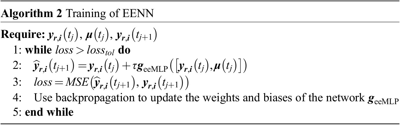
The algorithm for training such an EENN is provided in Algorithm 2 and the sketch of the network structure is given in Figure 3.
Picture of an explicit Euler neural network (EENN). EENN uses a multilayer perceptron (MLP) to approximate the R.H.S. of Equation (8). The output of the MLP is assembled as described in Equation (15).
3.3. Runge–Kutta neural network
We also consider in this work RKNN, which embed NNs into higher order numerical integration schemes. In this work, we only focus on explicit fourth-order Runge–Kutta (RK) as it is the most widely used version used in engineering problems, however the approach can be applied to any order. The fourth-order RK integration can be represented as follows:
where:
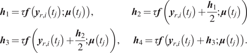
As we can see, the scheme requires the ability to evaluate the R.H.S. $ f\left(\boldsymbol{y},\mu \right) $
four times per time step. The concept of this approach is based on using a MLP NN to approximate this function
$ f\left(\boldsymbol{y},\mu \right) $
four times per time step. The concept of this approach is based on using a MLP NN to approximate this function
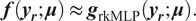 $$ \boldsymbol{f}\left({\boldsymbol{y}}_{\boldsymbol{r}};\boldsymbol{\mu} \right)\hskip2pt \approx \hskip2pt {\boldsymbol{g}}_{\mathrm{rkMLP}}\left({\boldsymbol{y}}_{\boldsymbol{r}};\boldsymbol{\mu} \right). $$
Then this MLP can be integrated into the RK scheme as subnetwork to obtain an integrator
where
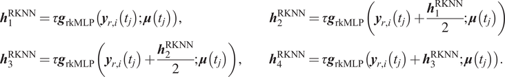
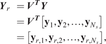
In Figure 4, we present a schematic on how the MLP subnetwork is embedded into the larger RKNN based on Equation (18). It is worth noticing that RKNNs also use a residual network structure.
Picture of a Runge–Kutta neural network (RKNN). An RKNN has a multilayer perceptron (MLP) as the core network which approximates the R.H.S. of Equation (8). The output of the network is assembled as described in Equation (16).
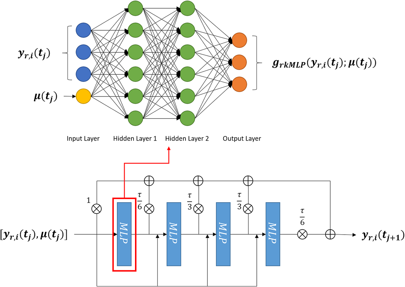
Let us take the computation of $ {\boldsymbol{h}}_1^{\mathrm{RKNN}} $
in Equation (18) as an example. We consider an MLP as subnetwork with one input layer, two hidden layers, and one output layer and all fully interconnected. The input layer receives the previous state vector
$ {\boldsymbol{h}}_1^{\mathrm{RKNN}} $
in Equation (18) as an example. We consider an MLP as subnetwork with one input layer, two hidden layers, and one output layer and all fully interconnected. The input layer receives the previous state vector $ {\boldsymbol{y}}_{r, i}\left({t}_j\right) $
and the parameter vector
$ {\boldsymbol{y}}_{r, i}\left({t}_j\right) $
and the parameter vector $ \boldsymbol{\mu} \left({t}_j\right) $
, that is the number of input neurons is set according to the number of components in the reduced space and the number of parameters. That is, the amount of neurons will depend exclusively on the model and it might change radically for different models. The output of this MLP becomes the approximation for
$ \boldsymbol{\mu} \left({t}_j\right) $
, that is the number of input neurons is set according to the number of components in the reduced space and the number of parameters. That is, the amount of neurons will depend exclusively on the model and it might change radically for different models. The output of this MLP becomes the approximation for $ {\boldsymbol{h}}_{\mathbf{1}} $
. The way subnetwork computing
$ {\boldsymbol{h}}_{\mathbf{1}} $
. The way subnetwork computing $ {\boldsymbol{h}}_2^{\mathrm{RKNN}},{\boldsymbol{h}}_3^{\mathrm{RKNN}} $
, and
$ {\boldsymbol{h}}_2^{\mathrm{RKNN}},{\boldsymbol{h}}_3^{\mathrm{RKNN}} $
, and $ {\boldsymbol{h}}_4^{\mathrm{RKNN}} $
are similar and the only difference is the reduced state vector
$ {\boldsymbol{h}}_4^{\mathrm{RKNN}} $
are similar and the only difference is the reduced state vector $ {\boldsymbol{y}}_{r, i}\left({t}_j\right) $
in the input will be replaced by
$ {\boldsymbol{y}}_{r, i}\left({t}_j\right) $
in the input will be replaced by
![]() , where
, where $ {c}_i $
is the coefficient in Equation (16) and
$ {c}_i $
is the coefficient in Equation (16) and $ {\boldsymbol{h}}_i^{\mathrm{RKNN}} $
is computed in previous iteration. The parameters of the subnetwork are updated using backpropagation. Also it is worth mentioning that although there will be multiple computation for the intermediate stages of the RK scheme, only one MLP subnetwork is needed for doing that. Therefore, the size of an RKNN is not affected by the order of the RK scheme.
$ {\boldsymbol{h}}_i^{\mathrm{RKNN}} $
is computed in previous iteration. The parameters of the subnetwork are updated using backpropagation. Also it is worth mentioning that although there will be multiple computation for the intermediate stages of the RK scheme, only one MLP subnetwork is needed for doing that. Therefore, the size of an RKNN is not affected by the order of the RK scheme.
Similar to explicit integrators, implicit ones can be used (Rico-Martinez and Kevrekidis, Reference Rico-Martinez and Kevrekidis1993). Due to their recurrent nature, or the dependence of predictions on themselves, the architecture of this type of NN will have recurrent connections and offer an alternative to the approach taken here.
4. Numerical Examples
In this section, the three numerical examples used for testing are described. The first one is a computer heat sink, which is governed by the thermal equation without any nonlinear contribution. The second one is a gap-radiation model whose physics equation is the thermal equation including fourth-order nonlinear radiation terms. And the last example is a thermal-fluid model simulating a heat exchanger, which includes the effects of fluid flow.
All test cases are all firstly reduced by POD method and then ROMs are evaluated by both MLP and RKNN. And to validate the ROMs, each example will be assigned two test cases, one is a constant-load test and the other one is a dynamic-load test.
The numerical experiments are performed on a computer with Intel Xeon E5-2640 CPU (6 cores and 2.50-3.00 GHz) and 48 GB memory. The snapshot simulations and reference solutions are provided by thermal/flow multi-physics module in simulation software Siemens Simcenter NX 12 (release 2020.1, version 1915).Footnote 1 The open-source machine learning library Pytorch (Paszke et al., Reference Paszke, Gross, Chintala, Chanan, Yang, DeVito, Lin, Desmaison, Antiga and Lerer2017) is used to realize the training of the NNs. Some special treatment to improve the network’s training is provided in Section 3.1, additionally, learning rate decay is employed to select the optimal learning rate adaptively. We also use early stopping (Prechelt, Reference Prechelt1998) to prevent the networks from overfitting.
4.1. Heat sink model
The first FEM model simulates a chip cooled by the attached heat sink. The chip will be the heat source of the system and heat flux travels from the chip to the heat sink then released into the environment through fins. Since the material used in the model is not temperature-dependent, the system is governed by the linear heat transfer equation as Equation (19).
where $ {\boldsymbol{C}}_{\boldsymbol{p}} $
is the thermal capacity matrix,
$ {\boldsymbol{C}}_{\boldsymbol{p}} $
is the thermal capacity matrix, $ \boldsymbol{K} $
is the thermal conductivity matrix,
$ \boldsymbol{K} $
is the thermal conductivity matrix, $ \boldsymbol{B} $
is the generalized load matrix,
$ \boldsymbol{B} $
is the generalized load matrix, $ \boldsymbol{T} $
is the state vector of temperature, and
$ \boldsymbol{T} $
is the state vector of temperature, and $ \boldsymbol{u} $
is the input heat load vector.
$ \boldsymbol{u} $
is the input heat load vector.
The meshed model is sketched in Figure 5a. The model consists of two parts, the red part is a chip made from copper whose thermal capacity is 385 J kg−1 K−1 and thermal conductivity is 387 W m−1 K−1. The green part represents the attached heat sink made from aluminum. The relevant material properties are 963 J kg−1 K−1 thermal capacity and 151 W m−1 K−1 thermal conductivity.
Test case: heat sink model.
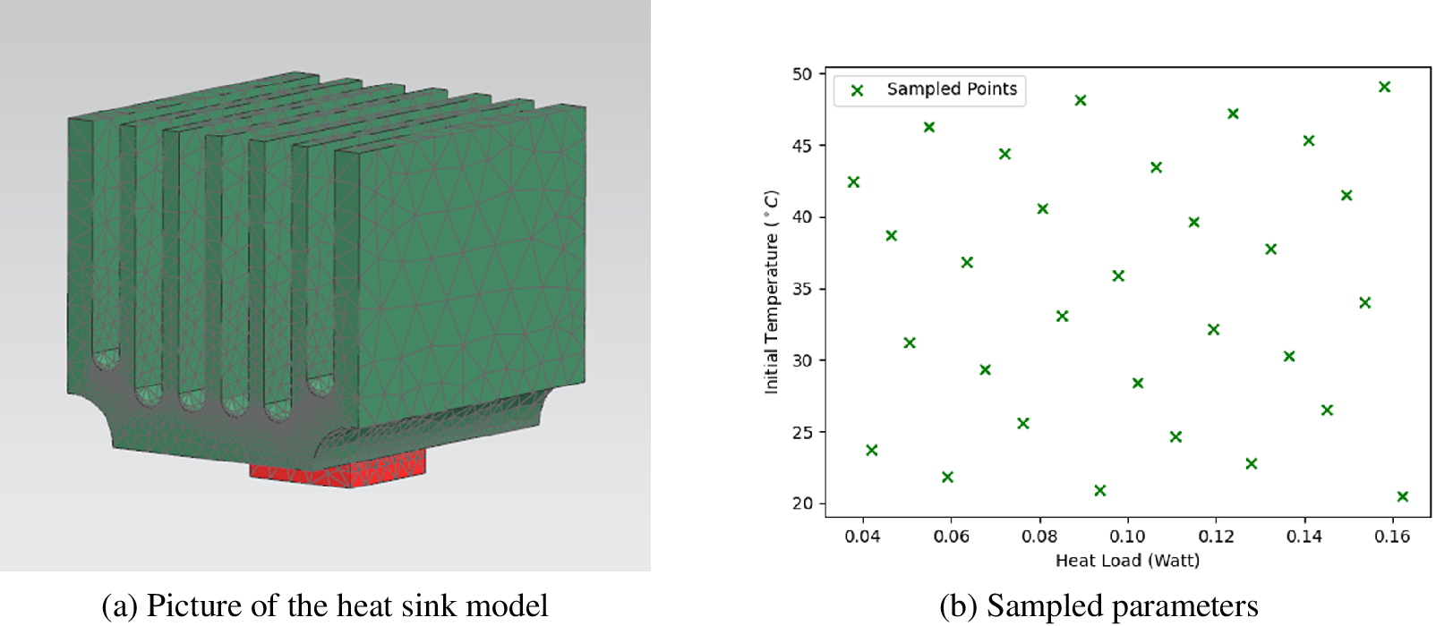
In the designed space, there are two variable parameters: initial temperature $ {T}_0 $
and input heat load
$ {T}_0 $
and input heat load $ u $
. The range of initial temperature is from 20°C to 50°C. The power of the volumetric heat source in the chip has range from 0.05 to 0.15 W/mm3. Parameter coordinates sampled in parameter space are shown in Figure 5b.
$ u $
. The range of initial temperature is from 20°C to 50°C. The power of the volumetric heat source in the chip has range from 0.05 to 0.15 W/mm3. Parameter coordinates sampled in parameter space are shown in Figure 5b.
Both test cases have uniform initial temperature of 20°C. The volumetric heat source used by constant-load test has fixed power 0.1 W/mm3 and the one used by dynamic-load test has power as function of time $ u(t)=0.15-0.1\frac{t}{500} $
W/mm3.
$ u(t)=0.15-0.1\frac{t}{500} $
W/mm3.
4.2. Gap-radiation model
The model presented here is a thermal model including radiative coupling. This model can be thought of as a proxy for other radiation-dominated heat transfer models such as those occurring in aerospspace, energy and manufacturing. The discrete governing equation is as Equation (20).
in addition to Equation (19), $ \boldsymbol{R} $
is the radiation matrix and the operation
$ \boldsymbol{R} $
is the radiation matrix and the operation $ {\left(\cdot \right)}^4 $
means to apply fourth-order power element-wise to the temperature vector, and not matrix multiplication.
$ {\left(\cdot \right)}^4 $
means to apply fourth-order power element-wise to the temperature vector, and not matrix multiplication.
The three-dimensional (3D) model is sketched in Figure 6a. As shown, the upper plate is heated by thermal flow. When the temperature equilibrium between the two plates is broken due to an increment of the temperature of the upper plate, radiative flux due to the temperature difference between two surfaces of the gap takes place.
Test case: gap-radiation model.
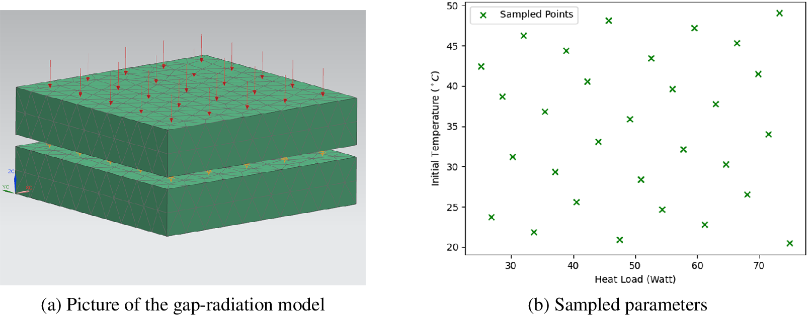
Both plates are made of steel, whose thermal capacity is 434 J kg−1 K−1 and thermal conductivity is 14 W m−1 K−1. The initial temperature $ {T}_0 $
and the applied heat load
$ {T}_0 $
and the applied heat load $ u $
are the variable parameters. The time scale of the whole simulated process is from 0 to 3,600 s.
$ u $
are the variable parameters. The time scale of the whole simulated process is from 0 to 3,600 s.
Assuming operation condition where the input heat load of the system has the lower limitation $ {u}_{min}=40\;\mathrm{W} $
and upper limitation
$ {u}_{min}=40\;\mathrm{W} $
and upper limitation $ {u}_{max}=60\;\mathrm{W} $
and the initial temperature has the lower limitation
$ {u}_{max}=60\;\mathrm{W} $
and the initial temperature has the lower limitation $ {T}_{0,\min }={20}^{\circ}\mathrm{C} $
and upper limitation
$ {T}_{0,\min }={20}^{\circ}\mathrm{C} $
and upper limitation $ {T}_{0,\max }={300}^{\circ}\mathrm{C} $
is investigated. So the parameter space to take snapshots is defined as
$ {T}_{0,\max }={300}^{\circ}\mathrm{C} $
is investigated. So the parameter space to take snapshots is defined as $ \left[{20}^{\circ}\mathrm{C},\hskip0.5em {300}^{\circ}\mathrm{C}\right]\times \left[40\mathrm{W},\hskip0.5em 60\mathrm{W}\right] $
. And the parameter configurations used for snapshots are given in Figure 6b.
$ \left[{20}^{\circ}\mathrm{C},\hskip0.5em {300}^{\circ}\mathrm{C}\right]\times \left[40\mathrm{W},\hskip0.5em 60\mathrm{W}\right] $
. And the parameter configurations used for snapshots are given in Figure 6b.
The test scenarios include a constant-load test and a dynamic-load test (Figure 7). The constant-load test has fixed load magnitude of 50 W, while the dynamic-load test has a time-dependent load magnitude $ u(t)=60-20\frac{{\left( t-1,800\right)}^2}{1,{800}^2} $
W.
$ u(t)=60-20\frac{{\left( t-1,800\right)}^2}{1,{800}^2} $
W.
Test case: heat exchanger model.
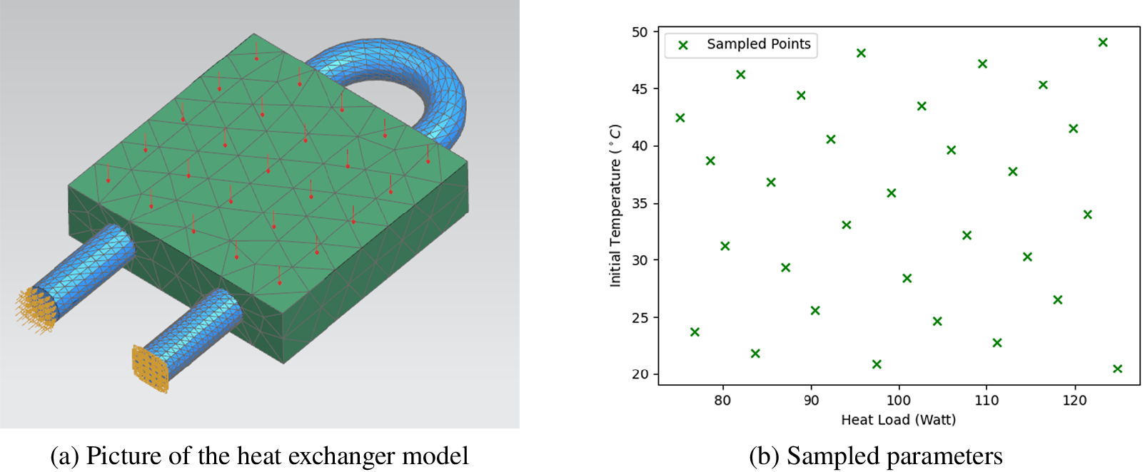
4.3. Heat exchanger model
In this example, we model the temperature profile of a solid that is in contact with a fluid channels to cool it down. The flow-field is governed by the Navier–Stokes (N–S) equations written in integral form (Kassab et al., Reference Kassab, Divo, Heidmann, Steinthorsson and Rodriguez2003):
where $ \Omega $
denotes the volume,
$ \Omega $
denotes the volume, $ \Gamma $
denotes the surface bounded by the volume
$ \Gamma $
denotes the surface bounded by the volume $ \Omega $
, and
$ \Omega $
, and $ n $
is the outward-drawn normal. The conserved variables are contained in
$ n $
is the outward-drawn normal. The conserved variables are contained in $ W=\left(\rho, \rho u,\rho v,\rho w,\rho e,\rho k,\rho \omega \right) $
, where,
$ W=\left(\rho, \rho u,\rho v,\rho w,\rho e,\rho k,\rho \omega \right) $
, where, $ \rho, u, v, w, e, k,\omega $
are the density, the velocity in x-, y-, and z-directions, and the specific total energy.
$ \rho, u, v, w, e, k,\omega $
are the density, the velocity in x-, y-, and z-directions, and the specific total energy. $ F $
and
$ F $
and $ T $
are convective and diffusive fluxes, respectively,
$ T $
are convective and diffusive fluxes, respectively, $ S $
is a vector containing all terms arising from the use of a noninertial reference frame as well as in the production and dissipation of turbulent quantities.
$ S $
is a vector containing all terms arising from the use of a noninertial reference frame as well as in the production and dissipation of turbulent quantities.
The governing equation for heat-conduction field in the solid is:
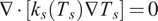 $$ \nabla \cdot \left[{k}_s\left({T}_s\right)\nabla {T}_s\right]=0 $$
here $ {T}_s $
denotes the temperature of the solid, and
$ {T}_s $
denotes the temperature of the solid, and $ {k}_s $
is the thermal conductivity of the solid material.
$ {k}_s $
is the thermal conductivity of the solid material.
Finally, the equations should be satisfied on the interface between fluid and solid are:
 $$ {T}_f={T}_s{k}_f\frac{\mathit{\partial}{T}_f}{\mathit{\partial} n}=-{k}_s\frac{\mathit{\partial}{T}_s}{\mathit{\partial} n} $$
here $ {T}_f $
is the temperature computed from N–S solution Equation (21) and
$ {T}_f $
is the temperature computed from N–S solution Equation (21) and $ {k}_f $
is thermal conductivity of fluid.
$ {k}_f $
is thermal conductivity of fluid.
The liquid flowing in the cooling tube is water whose thermal capacity is 4,187 J kg−1 K−1 and thermal conductivity is 0.6 W m−1 K−1. The fluid field has an inlet boundary condition which equals to 1 m/s. The solid piece is made of aluminum whose thermal capacity is 963 J kg−1 K−1 and thermal conductivity is 151 W m−1 K−1.
The initial temperature in the designed parameter space is from 20°C to 50°C and the heat load applied on the solid component varies from 80 to 120 W, as shown in Figure A1. Therefore, we will use a constant heat load whose magnitude is 100 W and a variant heat load whose magnitude is a function of time $ u(t)=120-0.8 t $
W to validate the ROM, respectively.
$ u(t)=120-0.8 t $
W to validate the ROM, respectively.
5. Results
In this section, the results of the numerical tests in Section 4 are presented. The comparison will be made along two dimension: the first dimension is sampling method, that is SPS versus DPS. The other dimension is architecture of NN, that is among MLP, EENN, and RKNN. Some qualitative and quantitative conclusion will be drawn based on comparison.
In Section 5.1, we will investigate how sampling strategy influences construction of reduced basis. And in Sections 5.2.1 and 5.2.2, we will focus on how dataset and architecture influences the learning quality respectively. For the investigation of different architectures, we focus on using MLPs and RKNNs to learn and predict with constant time step. In Section 5.2.3, we further study the capability of EENNs and RKNNs to learn from the snapshots sampled on the coarse time grids and to predict on the fine time grids.
5.1. POD reduction
With SPS and DPS respectively, 30 snapshots are taken for each system with 30 different heat-load magnitudes and initial temperatures. Each snapshot is a transient analysis from $ {t}_0=0 $
to
$ {t}_0=0 $
to $ {t}_{end} $
with 100 time points solved by NX 12.
$ {t}_{end} $
with 100 time points solved by NX 12.
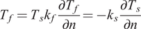
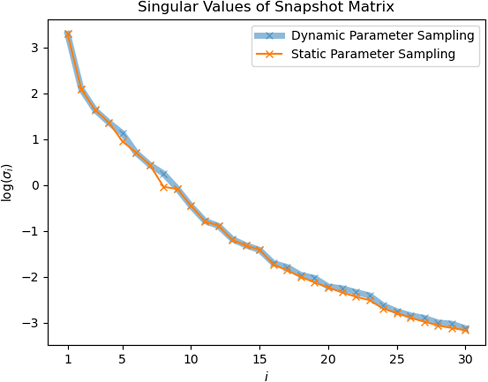
The first 30 singular values found from SPS snapshots and DPS snapshots are shown in Figures 8–10 for each test case respectively. In the heat sink test model, the curves of $ \sigma $
from calculated from different sampling strategies seem to exactly overlap on each other. And in Figures 9 and 10, only slight difference can be found between two curves.
$ \sigma $
from calculated from different sampling strategies seem to exactly overlap on each other. And in Figures 9 and 10, only slight difference can be found between two curves.
Heat sink model: singular values of static-parameter sampling (SPS) snapshots and dynamic-parameter sampling (DPS) snapshots.
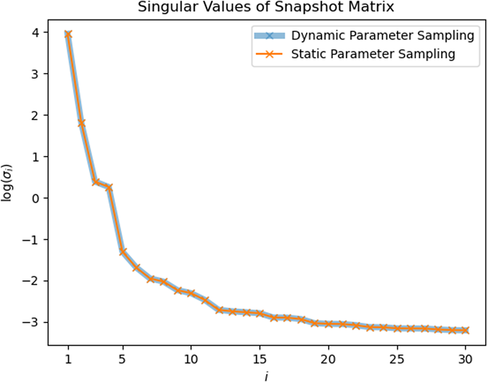
Gap-radiation model: singular values of static-parameter sampling (SPS) snapshots and dynamic-parameter sampling (DPS) snapshots.
Heat exchanger model: singular values of static-parameter sampling (SPS) snapshots and dynamic-parameter sampling (DPS) snapshots.
However, this does not mean the reduced basis constructed by different dataset has the same quality. To quantitatively measure the quality of reduced basis, here we perform re-projection test to calculate the error generated by each reduced basis. In the test, the reference trajectory is firstly projected into then reduced space then back-projected into the full space. This process can be done using $ {\hat{\boldsymbol{Y}}}_{ref}={\boldsymbol{VV}}^T{\boldsymbol{Y}}_{ref} $
. Depending on re-projected trajectory, we can calculate the relative re-projection error using
$ {\hat{\boldsymbol{Y}}}_{ref}={\boldsymbol{VV}}^T{\boldsymbol{Y}}_{ref} $
. Depending on re-projected trajectory, we can calculate the relative re-projection error using $ {E}_{POD}=\frac{1}{N_s\cdot k}\frac{{\left|{\boldsymbol{Y}}_{ref}-{\hat{\boldsymbol{Y}}}_{ref}\right|}_2}{{\left|{\boldsymbol{Y}}_{ref}\right|}_2} $
, where
$ {E}_{POD}=\frac{1}{N_s\cdot k}\frac{{\left|{\boldsymbol{Y}}_{ref}-{\hat{\boldsymbol{Y}}}_{ref}\right|}_2}{{\left|{\boldsymbol{Y}}_{ref}\right|}_2} $
, where $ {N}_s $
is number of snapshot simulations and
$ {N}_s $
is number of snapshot simulations and $ k $
is the number of time points in each simulation.
$ k $
is the number of time points in each simulation.
The POD errors with different sizes of reduced basis are shown in Figures A1 and A2. Similar to summarized above, in most situations, POD error curves generated by different sampling strategies can converge to similar values when the size of ROM is large enough. Nevertheless, in Figure Ab, the re-projection error of SPS-ROM converges to a value greater than DPS-ROM’s. This means the reduced basis calculated by DPS snapshots has higher quality (Figure A3).
It is observed that, SPS-ROM can have smaller projection error in some cases. This suggests that hybrid datasets (including static and dynamic parameters) may be needed to improve this aspect even further. We propose to study this possibility in future works.
5.2. ANN-based ROM
The quality of the ROM is affected by the reduced basis constructed by POD and the NN trained in the reduced space. In Section 5.1, by comparing singular values calculated from snapshot matrices sampled in different approaches, we did not see different sampling strategies have huge impact on constructing the POD subspace. But they can still make difference on training the NNs. This will be investigated in Section 5.2.1. In Section 5.2.2, we compare MLP and RKNN with constant-step-size tests. In Section 5.2.3, we compare EENN with RKNN with variant-step-size tests.
5.2.1. Static-parameter sampling versus dynamic-parameter sampling
In Section 2.2, we introduced two approaches for taking snapshots. In conventional SPS, the parameter configuration assigned to the system is constant during the simulation time, that is $ \boldsymbol{\mu} (t)={\boldsymbol{\mu}}_0 $
. To include more parameter diversity in training data, we designed new sampling strategy named DPS whose parameter configuration is function of time. Datasets sampled by different strategies influences not only the quality of reduced basis but also the training of NN. In this section, how different datasets can affect the training is investigated.
$ \boldsymbol{\mu} (t)={\boldsymbol{\mu}}_0 $
. To include more parameter diversity in training data, we designed new sampling strategy named DPS whose parameter configuration is function of time. Datasets sampled by different strategies influences not only the quality of reduced basis but also the training of NN. In this section, how different datasets can affect the training is investigated.
To measure the prediction quality of the NNs correctly, the influence of reduction projection will be removed from measurement. In other words, the approximation error should be evaluated in the reduced space. Therefore, the reference trajectory is reduced by $ {\boldsymbol{Y}}_{\boldsymbol{r} ref}={\boldsymbol{V}}^{\boldsymbol{T}}{\boldsymbol{Y}}_{ref} $
. With the prediction
$ {\boldsymbol{Y}}_{\boldsymbol{r} ref}={\boldsymbol{V}}^{\boldsymbol{T}}{\boldsymbol{Y}}_{ref} $
. With the prediction $ {\tilde{\boldsymbol{Y}}}_{\boldsymbol{r}} $
made by NN, the relative approximation error is calculated as
$ {\tilde{\boldsymbol{Y}}}_{\boldsymbol{r}} $
made by NN, the relative approximation error is calculated as
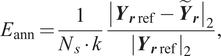 $$ {E}_{\mathrm{ann}}=\frac{1}{N_s\cdot k}\frac{{\left|{\boldsymbol{Y}}_{\boldsymbol{r}\mathrm{ref}}-{\tilde{\boldsymbol{Y}}}_{\boldsymbol{r}}\right|}_2}{{\left|{\boldsymbol{Y}}_{\boldsymbol{r}\mathrm{ref}}\right|}_2}, $$
where $ {N}_s $
is number of snapshot simulations and
$ {N}_s $
is number of snapshot simulations and $ k $
is the number of time points in each simulation.
$ k $
is the number of time points in each simulation.
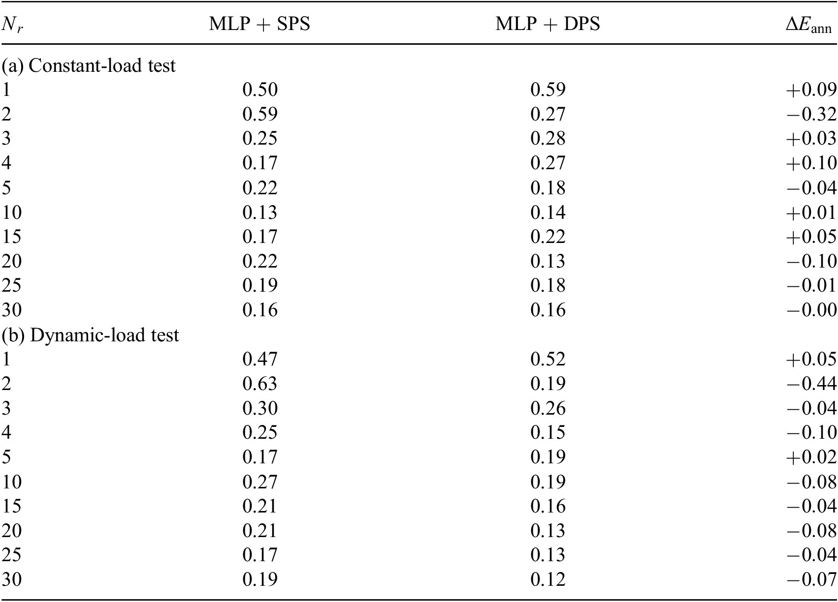
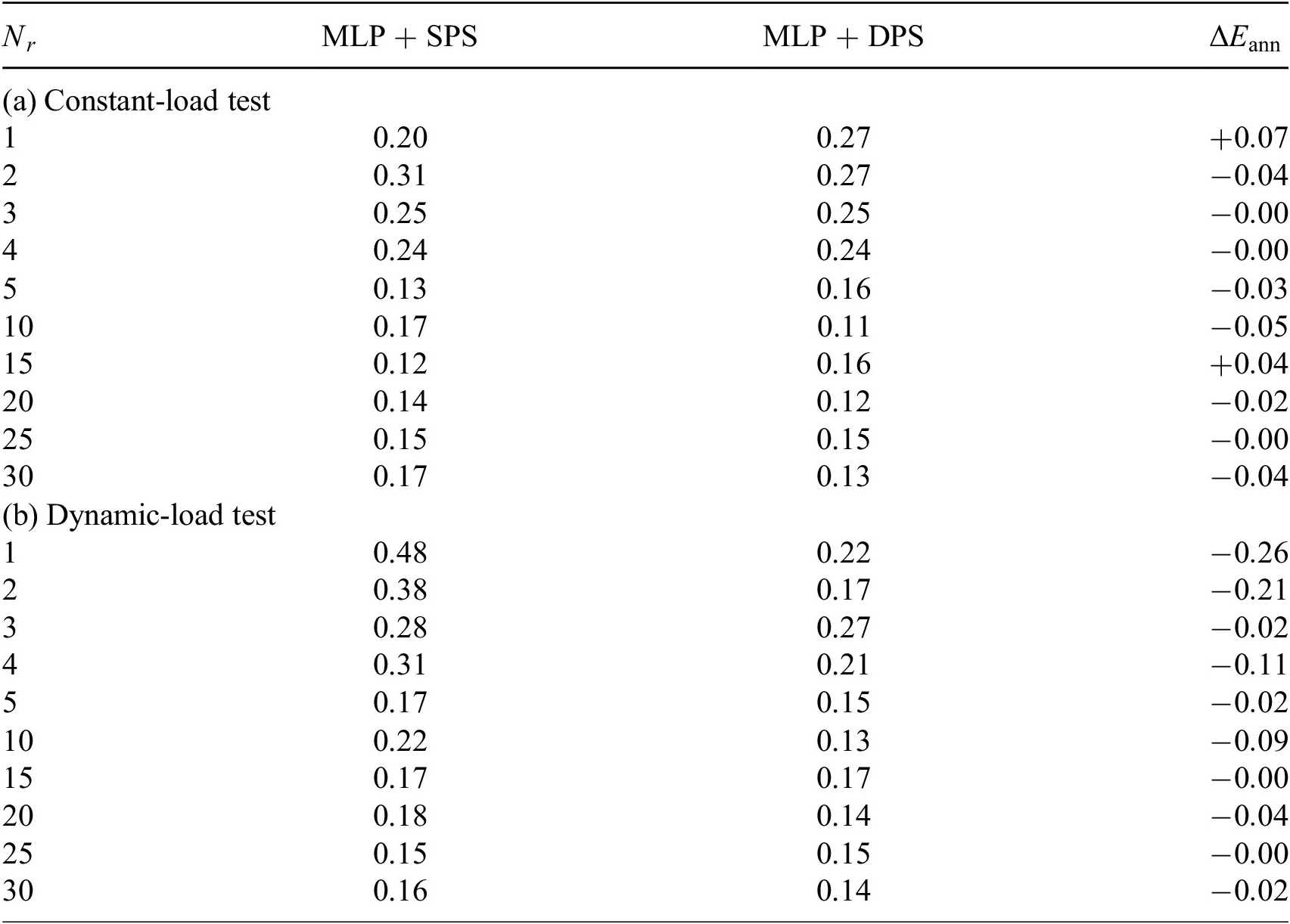
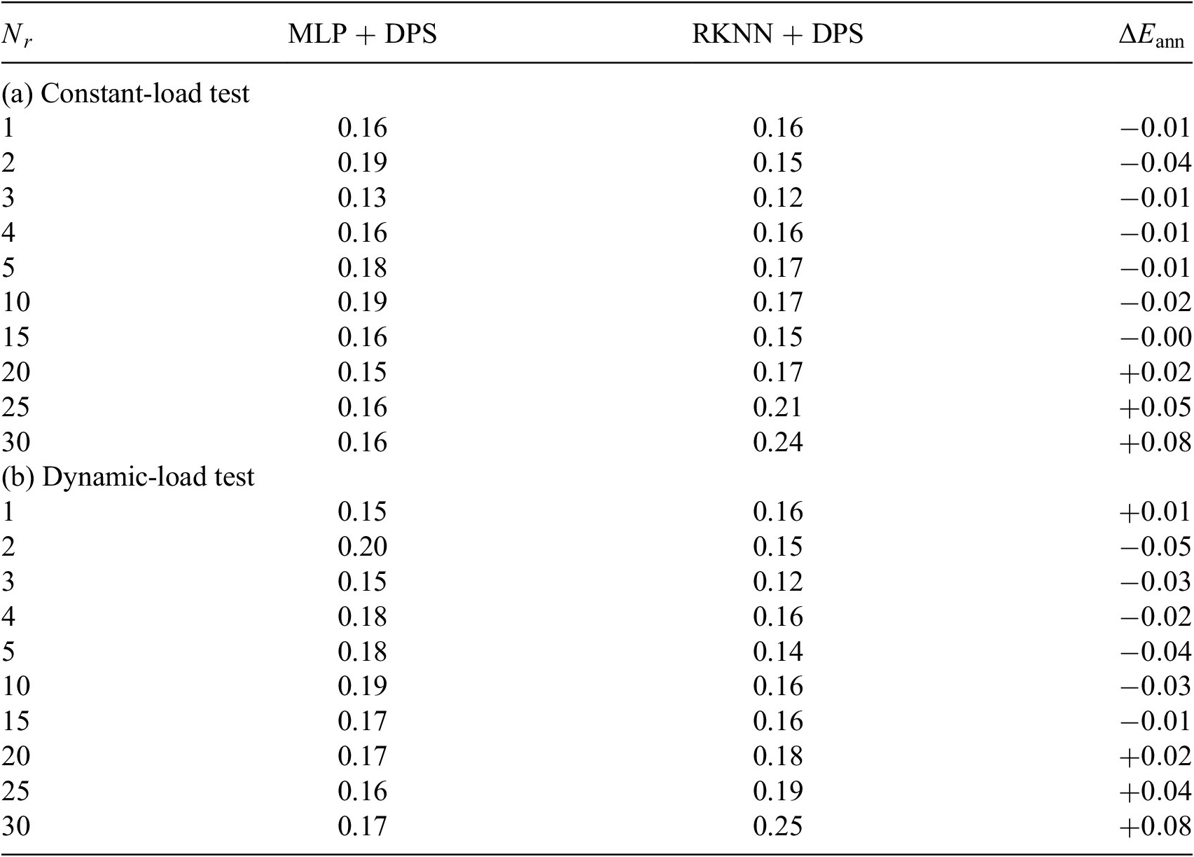
In Tables 1–4, we list the reference tests on the left and their competitors are listed on the right. The values $ \Delta {E}_{\mathrm{ann}} $
stand for how much the relative prediction errors increase or decrease by using the competitive approaches. This notation is also used in the later tables. It is observed that in 45 out of 60 (3/4) test cases ROMs trained by DPS data predict better in both test cases. But unlike many other MOR methods, the simulation error does not monotonically decrease while increasing the size of the ROM. When the ROM size is small, the simulation error is mainly caused by POD projection error. In this region, simulation error will decrease with increasing ROM size. Because the most dominant POD components are the most important physics modes of the system, by adding them the ROM knows more about the original system. However, POD components with smaller singular values might be trivial information in snapshots, for example, noise from numerical integration. These trivial information also becomes noise in training data and disturbs the learning process. This also reminds us to be careful to choose the size of ROM while using ANN-based MOR techniques.
$ \Delta {E}_{\mathrm{ann}} $
stand for how much the relative prediction errors increase or decrease by using the competitive approaches. This notation is also used in the later tables. It is observed that in 45 out of 60 (3/4) test cases ROMs trained by DPS data predict better in both test cases. But unlike many other MOR methods, the simulation error does not monotonically decrease while increasing the size of the ROM. When the ROM size is small, the simulation error is mainly caused by POD projection error. In this region, simulation error will decrease with increasing ROM size. Because the most dominant POD components are the most important physics modes of the system, by adding them the ROM knows more about the original system. However, POD components with smaller singular values might be trivial information in snapshots, for example, noise from numerical integration. These trivial information also becomes noise in training data and disturbs the learning process. This also reminds us to be careful to choose the size of ROM while using ANN-based MOR techniques.
SPS versus DPS: heat sink model, relative error(%).

Abbreviations: DPS, dynamic-parameter sampling; MLP, multilayer perceptron; SPS, static-parameter sampling.
SPS versus DPS: gap-radiation model, relative error(%).
Abbreviations: DPS, dynamic-parameter sampling; MLP, multilayer perceptron; SPS, static-parameter sampling.
SPS versus DPS: heat exchanger model, relative error(%).
Abbreviations: DPS, dynamic-parameter sampling; MLP, multilayer perceptron; SPS, static-parameter sampling.
MLP versus RKNN: heat sink model, relative error(%).
Abbreviations: DPS, dynamic-parameter sampling; MLP, multilayer perceptron; RKNN, Runge–Kutta neural network.
The tests here are considered as independent tests since test datasets are provided by new NX simulation with different parameter configuration from the simulations used in the snapshots. The independent test is optimal if the two datasets originate from two different sampling strategies (Özesmi et al., Reference Özesmi, Tan and Özesmi2006). Here, dynamic-load test can be considered to be optimal independent test for SPS-ROM and vice versa for DPS-ROM. As shown in Tables 1–4, the ANNs trained by DPS data have better performance on most of its optimal independent tests. But ANNs trained by SPS data also outperforms in some test cases. This result reminds us again that using dataset obtained from diverse sources should be considered.
5.2.2. Constant-time-grid learning: MLP versus RKNN
To further improve the capability of predicting ODE systems, we propose to use network architecture inspired by RK integrator in Section 3.3. Although it has been previously seen that RKNN can be used to make long-term predictions for ODE system (Wang and Lin, Reference Wang and Lin1998), it is still not clear if such approach can work for POD-projected ODE systems. A possible challenge arises from the highly variable scale differences between the reduced dimensions. Typically, the reduced snapshot will have much larger component in some of the reduced dimensions (those with large singular values) than in others (small singular values). This presents a challenge for NN-based learning methods.
The structure of MLP and RKNN is the same as described in Figures 2 and 4, but in detail, the number of input neurons $ {n}_{in} $
depends on the size of ROM and number of system parameters, that is
$ {n}_{in} $
depends on the size of ROM and number of system parameters, that is
![]() . The number of neurons on each hidden layers is chosen to be
. The number of neurons on each hidden layers is chosen to be $ 32 $
, this value is always greater than input features, that is
$ 32 $
, this value is always greater than input features, that is
![]() . This is important for NN to interpret the underlying dynamics. And same as depicted in the figures, each network has one input layer, two hidden layers, and one output layer, which enables network to approximate any kind of mathematical function.
. This is important for NN to interpret the underlying dynamics. And same as depicted in the figures, each network has one input layer, two hidden layers, and one output layer, which enables network to approximate any kind of mathematical function.
The prediction error $ {E}_{ann} $
is measured in the same way as in Section 5.2.1. Since it is known from the last comparison that DPS dataset is considered to be better training dataset, here both types of NNs are trained with DPS dataset. And for each test case, the time grids used for collecting snapshots and for validation have the same resolution. For these grids, 100 points are uniformly distributed on the time axis. This time resolution can be considered to be fine to the nature of the test systems. Therefore, the learning task in this section can be considered as learning from a fine time grid compared to the learning task in the next section.
$ {E}_{ann} $
is measured in the same way as in Section 5.2.1. Since it is known from the last comparison that DPS dataset is considered to be better training dataset, here both types of NNs are trained with DPS dataset. And for each test case, the time grids used for collecting snapshots and for validation have the same resolution. For these grids, 100 points are uniformly distributed on the time axis. This time resolution can be considered to be fine to the nature of the test systems. Therefore, the learning task in this section can be considered as learning from a fine time grid compared to the learning task in the next section.
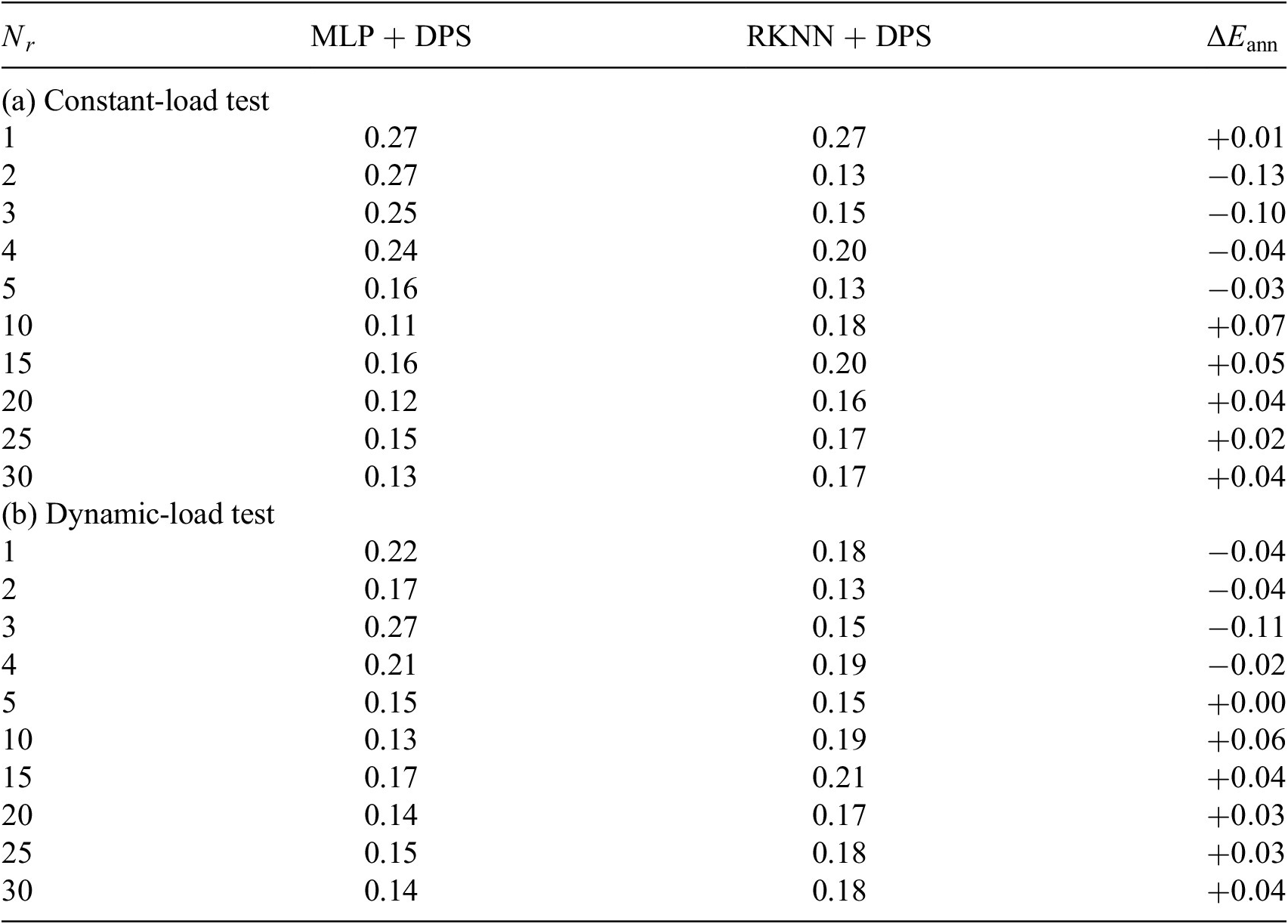
In Tables 5 and 6, we can observe that RKNN can predict the solution of reduced ODE system with acceptable accuracy. But there is no indication that RKNN predicts the system behavior better in any certain type of tests. In contrast, MLP is evaluated to be better at approximating larger-size ROM. One possible explanation is that compared to a simple MLP, an RKNN can be considered as a deeper network which is harder to train (Du et al., Reference Du, Lee, Li, Wang and Zhai2019). A solution could be to train large amount of networks for each architecture but with different randomized initialization. Then evaluating the average performance of all trained networks of each architecture. Here in this paper, due to the limitation of time and computational resource, we only train 10 networks for each type of architecture, which might not be sufficient to eliminate the random effect.
MLP versus RKNN: gap-radiation model, relative error(%).

Abbreviations: DPS, dynamic-parameter sampling; MLP, multilayer perceptron; RKNN, Runge–Kutta neural network.
MLP versus RKNN: heat exchanger model, relative error(%).
Abbreviations: DPS, dynamic-parameter sampling; MLP, multilayer perceptron; RKNN, Runge–Kutta neural network.
5.2.3. Coarse-time-grid learning: EENN versus RKNN
Although the results of the previous section are inconclusive to demonstrate the advantages of RKNN over MLP, here we will analyze a practical advantage of learning the system dynamics (learning $ \boldsymbol{f}\left(\cdot \right) $
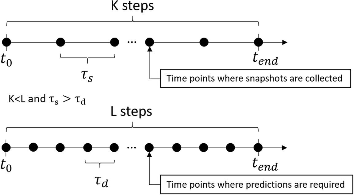
) compared to directly learning the evolution of the system state. In the former case, the time step size for prediction can be chosen independently of the time step used to take the snapshots. In this section, we use a training data set in which snapshots are sampled coarsely, that is with a large time interval, to build new ROMs. Then we evaluate the capability of these ROMs to predict the time evolution of the system under new parameters and using finer integration time steps. Such a scenario is relevant in the context of MOR when the FOMs are very large, as time and memory constraints might limit the amount of (full order) input data available to provide to the MOR methods.
$ \boldsymbol{f}\left(\cdot \right) $
) compared to directly learning the evolution of the system state. In the former case, the time step size for prediction can be chosen independently of the time step used to take the snapshots. In this section, we use a training data set in which snapshots are sampled coarsely, that is with a large time interval, to build new ROMs. Then we evaluate the capability of these ROMs to predict the time evolution of the system under new parameters and using finer integration time steps. Such a scenario is relevant in the context of MOR when the FOMs are very large, as time and memory constraints might limit the amount of (full order) input data available to provide to the MOR methods.
MLPs (as defined in Section 3.1) cannot be applied to this test as we cannot use an independent time step for evaluation. Therefore, we consider only EENNs and RKNNs. For examples in which the training and evaluation time steps are equivalent, we expect EENNs to be equivalent to MLPs (Figure 11).
Time grid for collecting snapshots and time grid for prediction with reduced order model (ROM).
In the experiments, we prepare two dataset. For the dataset A, $ K=25 $
snapshots are collected in each snapshot simulation with DPS. For the purpose of validation, ROMs are asked to predict in the same time span but with
$ K=25 $
snapshots are collected in each snapshot simulation with DPS. For the purpose of validation, ROMs are asked to predict in the same time span but with $ L=\mathrm{25,50,100,200,300,500,1},000 $
steps. To be more specific, if the step size used in training dataset is
$ L=\mathrm{25,50,100,200,300,500,1},000 $
steps. To be more specific, if the step size used in training dataset is $ {\tau}_s $
, the step size used in validation is
$ {\tau}_s $
, the step size used in validation is $ {\tau}_d={\tau}_s,{\tau}_s/2,\dots, {\tau}_s/20,{\tau}_s/40 $
. In the dataset B,
$ {\tau}_d={\tau}_s,{\tau}_s/2,\dots, {\tau}_s/20,{\tau}_s/40 $
. In the dataset B, $ K=100 $
snapshots are collected in each snapshot simulation. The trained ROMs will predict in the same time span with
$ K=100 $
snapshots are collected in each snapshot simulation. The trained ROMs will predict in the same time span with $ L=\mathrm{100,200,300,500,1},000 $
steps. The reduced data in both training sets has the size of 10. The ROMs with such a size are observed to be stable with the POD projection error according to the previous tests. And we use DPS to collect the data since it generally collects more information.
$ L=\mathrm{100,200,300,500,1},000 $
steps. The reduced data in both training sets has the size of 10. The ROMs with such a size are observed to be stable with the POD projection error according to the previous tests. And we use DPS to collect the data since it generally collects more information.
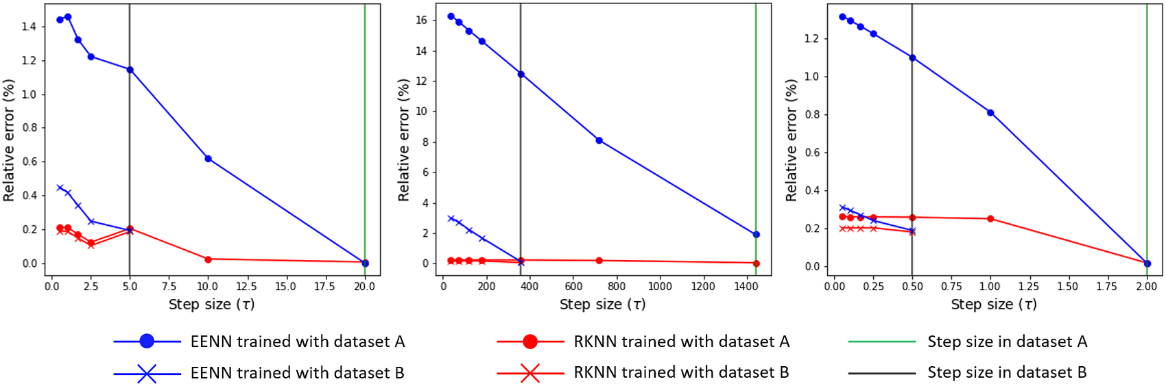
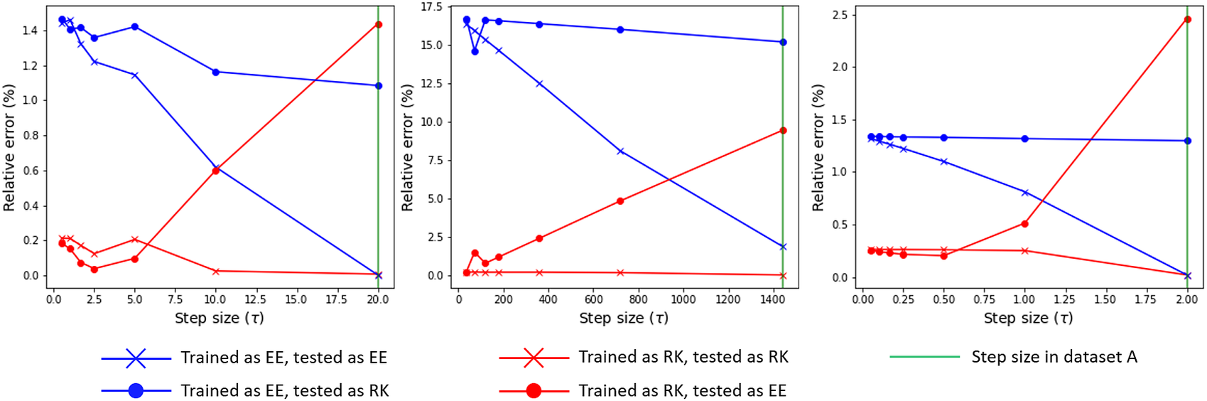
Figure 12 presents the results of this comparison. Each of the plots corresponds to a different test model from Section 4 and they show the relative errors, calculated according to Equation (24) for prediction at different time step sizes. For the reference (training) time step, the errors are small and comparable for both EENN and RKNN, which is consistent with the observations in Section 5.2.2. For smaller evaluation time steps, the errors become larger. We speculate that the learned R.H.S. still contains information from the time step size used during training. However, we can clearly see that this effect is consistently smaller for RKNN-MOR. This suggests that the use of the higher order numerical scheme during training can provide a better quality inferred R.H.S.
The graph from the left to the right belongs to the heat sink model, the gap-radiation model and the heat exchanger model respectively. The reduced order model (ROMs) are generated from the coarse and the fine time grids respectively. The prediction is made with time steps which are always finer than the step sizes used in training data. The original step sizes used in two training snapshots are marked with green (dataset A) and black (dataset B) vertical lines.
To further explore this hypothesis we can perform an additional test of the trained ROMs. As both EENN and RKNN learn the right side $ \boldsymbol{f}\left(\cdot \right) $
of Equation (8), we can integrate the ROM with a different numerical scheme as the training. Results of these tests are presented in Figure 13, where we plot these tests alongside the data in Figure 12. The new data includes the following: (a) the error incurred from integrating the EENN-ROM using RK scheme and (b) the error incurred from integrating the RKNN-ROM using EE scheme. The same qualitative behavior is observed for all test models. Interestingly, the error is almost always largest and roughly independent of the step size when using RK scheme to integrate the EENN-ROM. For RKNN-ROMs evaluated using EE scheme, the trend is quite different. For the original (large) time step sizes, the errors are always larger than the reference RKNN results. However, for smaller evaluation time steps the error approaches the same values as the result of integrating using RK scheme.
$ \boldsymbol{f}\left(\cdot \right) $
of Equation (8), we can integrate the ROM with a different numerical scheme as the training. Results of these tests are presented in Figure 13, where we plot these tests alongside the data in Figure 12. The new data includes the following: (a) the error incurred from integrating the EENN-ROM using RK scheme and (b) the error incurred from integrating the RKNN-ROM using EE scheme. The same qualitative behavior is observed for all test models. Interestingly, the error is almost always largest and roughly independent of the step size when using RK scheme to integrate the EENN-ROM. For RKNN-ROMs evaluated using EE scheme, the trend is quite different. For the original (large) time step sizes, the errors are always larger than the reference RKNN results. However, for smaller evaluation time steps the error approaches the same values as the result of integrating using RK scheme.
The graph from the left to the right belongs to the heat sink model, the gap-radiation model and the heat exchanger model respectively. The tests aim to evaluate the accuracy of the learned reduced order model (ROMs) in.
We can interpret these trends as follows: for the RKNN-ROM (red curves), we see that evaluating using EE scheme (circle markers) gives larger errors than RK scheme (cross markers) for large time steps, but that the error converges for smaller time steps. This is consistent with having an accurate R.H.S. and integrating it using a higher or lower order integration scheme. For the EENN-ROM (blue curves), the error is almost always larger than for RKNN-ROM and its convergence trend also contradicts the result that we would observe with a real analytical R.H.S. Additionally, the errors become small only while matching the evaluation conditions with the training conditions. This is consistent with our hypothesis that the R.H.S. learned by EENNs are more influenced by the time step size in the training data, therefore having less flexibility for changing it.
In summary, we believe that these tests strongly suggest that the use of higher order integration schemes during training can noticeably improve the quality of the dynamics learned in the reduced space, especially when the input data is sampled sparsely.
6. Conclusions
In this paper, we investigated different varieties of MOR based on ANN. In the first part, we looked at different ways of generating the training data, namely SPS versus DPS. In the second part, we study the influence of using different NN architectures. We compared MLP NNs that directly learn the evolution of the system state with RKNN which learn the R.H.S. of the systems. Besides, we compared RKNN versus EENN which learns the system R.H.S. similarly but with lower-order numerical scheme, with a focus on the effect on learning reduced models from sparsely sampled data.
As discussed in Section 5.2.1, DPS shows positive influence on the quality of ROM. Based on observation, adding DPS snapshots into the dataset can enrich the dynamics contained in snapshots. This can help with constructing better POD basis. Moreover, NN trained by DPS dataset is more sensitive to system’s parameters. However, it is also seen that in some specific tests, network trained by DPS data performs worse than networks trained by SPS data, which are usually found to be in the constant-load tests. However, the direct comparison of RKNN and MLP did not show clear advantage of either architecture under the conditions of the tests in Section 5.2.2.
The advantage of RKNN could actually be demonstrated by analyzing a test case in which the training dataset is sampled coarsely in time. Here, we observed, that RKNN can predict with different step sizes without significant increment of the prediction error. In contrast, this was not the case for EENN. Our results also suggest that embedding a higher order integration scheme can help learning the systems dynamics more reliably and independently of the time step in the input data. This result is relevant for engineering applications, where memory and computational time constraints can limit the amount of data made available for MOR.
Although this MOR framework was tested only on thermal and thermal-flow models, it could be easily adapted to other kinds of models, since it is nonintrusive and only relies on measured data to learn the dynamics of the system. However, there is still more work to be done before these methods can be applied to big scale and more general models.
Some further potential improvements for the approach discussed in this work include:
-
• Investigating the influence of using SPS–DPS-mixed snapshots.
-
• Investigating different methods of constructing reduced space other than POD, for example, auto-encoder.
-
• Implementing implicit integration scheme with NNs as in Anderson et al. (Reference Anderson, Kevrekidis and Rico-Martinez1996) allowing more accurate long-term prediction.
-
• Implementing integration scheme with multiple history states as part of input, which might also enable more stable long-term prediction.
Acknowledgments
The authors are grateful to Siemens for sponsoring this project. The authors also thank Prof. Benjamin Peherstorfer and Lukas Failer for their valuable suggestions for the research.
Funding Statement
This work is part of the research undertaken by the authors in COMPAS which is an ITEA-EUREKA project co-funded by the Federal Ministry of Education and Research of Germany (BMBF).
Competing Interests
Q.Z., J.L., and D.H. are employed at company Siemens AG.
Data Availability Statement
To get access to research data, please contact one of the authors with your request.
Author Contributions
Conceptualization: D.H. and H.-J.B.; Methodology: D.H., Q.Z., and J.L.; Data curation: Q.Z.; Data visualization: Q.Z.; Writing-original draft: Q.Z., J.L., and. D.H. All authors approved the final submitted draft.
Appendix: Additional Figures
Projection error: heat sink model.
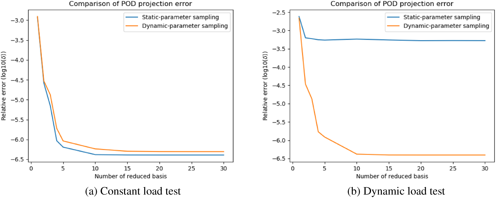
Projection error: gap-radiation model.
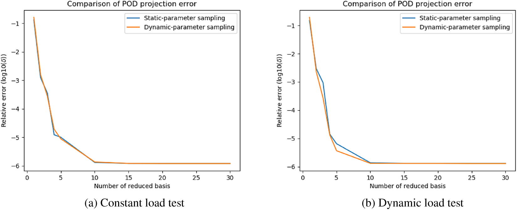
Projection error: heat exchanger model.
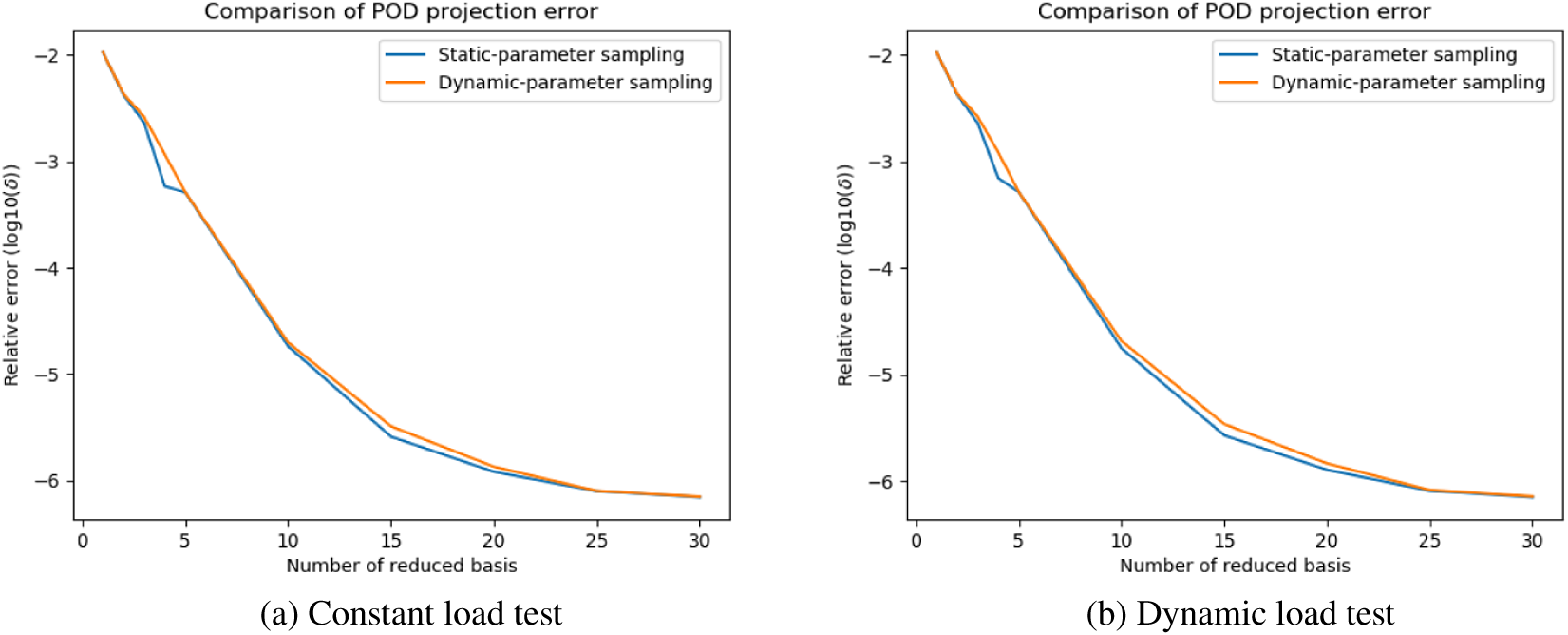


 Open access
Comments
No Comments have been published for this article.