





Impact Statement
A data driven strategy to split grayscale intensity histogram of an image into constituent Gaussians is presented here. Though several techniques exist, accurate ones are expensive, needing large amounts of training data, active labelling, several hours of human time, etc. This work alleviates the demand for such resources — requiring very little training data, significantly less human time, albeit still allowing the user to “guide” the segmentation and reach accuracy comparable with active-labelling methods. Mathematically, this work builds up on CIGSCR – an iterative clustering approach that minimizes within-cluster weighted variance, producing new clusters by splitting/merging existing clusters via a test-statistic, guided by the available training data. This work will be useful in applications that analyze images of materials, e.g., Digital Rock, carbon storage management (micro-CT rock scans to explore carbon storing potential), new energies (scans of alloys to analyze their structure/artefacts/composition), water resource management, catalysis.
1. Introduction
Segmentation of digital images of materials is of great importance in many applications such as carbon sequestration and storage (CSS), hydrocarbon explorations, nature-based solutions (NBS) for energy transition (Hirscher et al., Reference Hirscher, Yartys, Baricco, Bellosta von Colbe, Blanchard, Bowman, Broom, Buckley, Chang, Chen, Cho, Crivello, Cuevas, David, de Jongh, Denys, Dornheim, Felderhoff, Filinchuk, Froudakis, Grant, Gray, Hauback, He, Humphries, Jensen, Kim, Kojima, Latroche, Li, Lototskyy, Makepeace, Møller, Naheed, Ngene, Noréus, Nygård, ichi Orimo, Paskevicius, Pasquini, Ravnsbæk, Veronica Sofianos, Udovic, Vegge, Walker, Webb, Weidenthaler and Zlotea2020), underground water management, and the like. The structure and composition of these materials are complex and unpredictable. Understanding this composition and associated properties at pore-level influences research directions, technology designs, and key business decisions. For over a decade now, advances in imaging technologies are enabling acquisition and visualization of structures in materials with very high level of details. Harnessed well, these images have the potential to provide unprecedented detailed level of understanding of material structures. Multiphase segmentation of a digital material image refers to identification and labeling of the numerous phases of interest (e.g., void space, pore-filling fluids, unresolved porosity, minerals, alloys, compounds, grain-grain interface deposits/films, and the like) present in that material.
Popular modalities used for acquiring digital images of materials include computed tomography (CT) scanners, scanning electron microscopes (SEM), transmission electron microscopes (TEM), and synchrotrons. Of these, micro-CT scans form a popular resource for investigating various descriptive and quantitative properties of several materials. For rocks, Micro-CT images are grayscale volumetric images and have several advantages over other imaging modalities: they provide holistic 3D visualization of rock samples, with fit-for-purpose resolution (micrometer level, a level at which internal structures, pore networks, and other features of interest in a rock are resolved while still keeping a representative field of view), are nondestructive in nature, and laboratory-based imaging systems are readily available for commercial purposes. Micro-CT scans are very popular in hydrocarbon explorations (Digital Rock Physics [DRP], an emerging technology that aims to complement the traditional laboratory-based petrophysical measurements, albeit with orders of magnitude shorter analysis time). Micro-CT images of rocks are also being used for estimating the carbon sequestration potential of rocks (Callow et al., Reference Callow, Falcon-Suarez, Ahmed and Matter2018), the latter being widely explored as a strategy for mitigating CO2 emissions.
Though literature is replete with segmentation algorithms, accurate segmentation of images of materials continues to be a challenging task. In the context of micro-CT rock images, for example, the grayscale units produced by micro-CT instruments differ from one sample to another and between facilities. Further, rocks often contain very high-density minerals (typically, with low spatial extent). The presence of such high-density minerals offsets the grayscale measures, with high attenuation coefficient grains occupying high-grayscale ranges and all the rest of the grains being compressed to a relatively small range of grayscale values. Consequently, several (low density) minerals can have very similar grayscale value, which leads to nonunique solution to the segmentation problem (Karimpouli and Tahmasebi, Reference Karimpouli and Tahmasebi2019). The list of challenges can be further expanded. Several unsupervised algorithms have been utilized for multiphase segmentation of micro-CT images (MacQueen, Reference MacQueen1967; Otsu, Reference Otsu1979). Unfortunately, these often lead to inaccurate separation of mineral phases for images of materials. Supervised algorithms (e.g., convolutional neural network [CNN]-based semantic segmentation) are generally more accurate but the accuracy comes at the cost of a significant amount of training as well as large computational resources. Obtaining large amounts of training data for rock samples necessitates extensive involvement of a trained human agent, making the process very expensive (Zhao, Reference Zhao2017).
Semisupervised learning is an approach to machine learning that utilizes unlabeled data in addition to labeled data, together with additional/secondary criterion to achieve classification. Semisupervised learning algorithms assume that data exists in clusters and that data points that are close to each other are more likely to share a label. Examples of additional clustering criterion used from literature include relating the properties of the distributions comprising the input with the properties of the decision function, introducing “must-link” and “cannot-link” constraints into an optimization problem (e.g., Belkin and Niyogi, Reference Belkin and Niyogi2004), and the like. Semisupervised learning approach falls in between unsupervised and supervised (a hybrid of the two) learning approaches. When training data is less, semisupervised learning helps in supplementing labeled training data, thus mitigating the problem of overfitting. Works such as Jeon and Landgrebe (Reference Jeon and Landgrebe1999) and Chi and Bruzzone (Reference Chi and Bruzzone2005) focus on generating multiclass segmentation labels when class labels for only a few classes are provided. Semisupervised learning has received attention for image segmentation as well. Remotely sensed images are characterized by limited training data availability and semisupervised algorithms have shown significant improvement in performance in segmentation of these images (Wayman et al., Reference Wayman, Wynne, Scrivani and Reams2001). A secondary advantage of semisupervised algorithms is also that these approaches allow a high level of automation compared to strictly supervised algorithms.
This work proposes a semisupervised clustering approach toward multiphase segmentation of digital scans of materials. A semisupervised framework named Continuous Iterative Guided Spectral Class Rejection (CIGSCR) was originally published by Phillips et al. (Reference Phillips, Watson and Wynne2011). CIGSCR is utilized and analyzed for images of materials here. Micro-CT images arising in DRP are utilized as the use case. Developed closely with domain experts, the current implementation is tested over a benchmark dataset as well as across rocks from multiple geological formations. The challenge lay in designing an approach that was context free and could handle the unpredictability of unseen data. Unlike hyperspectral images used in Phillips et al. (Reference Phillips, Watson and Wynne2011), micro-CT images are monospectral. In addition, while EO images are two-dimensional images of a surface, micro-CT images are three-dimensional volumetric images. This paper demonstrates that the approach offers very promising results for rock images. Further, by providing training data only from one slice (say, the center slice) of an image volume, segmentation of the full volume can be attained, including minerals that were not present in the training data. The segmentation obtained is accurate up to the uniqueness of the grayscale values of the image. Scalability to data sizes that are meaningful to DR is briefly discussed. To our knowledge, semisupervised learning algorithms have not been explored for images of materials. Though most discussions in this article refer to micro-CT scans of rocks, the approach is expected to extend naturally to other materials (e.g., catalysts, alloys) and SEM scans as well.
The rest of this report is organized as follows. Section 2 presents an overview of literature on segmentation approaches relevant to DRP. Section 3 describes CIGSCR, the algorithm proposed for multiphase segmentation. Description of input data used for this work is presented in Section 4. Section 5 presents representative experimental results and Section 6, a discussion of the results. Section 7 presents discussions on scalability and CIGSCR iterations. Conclusions are provided in Section 8.
2. Background
Conventional segmentation algorithms range from simple thresholding to multi-step marker-based methods. These methods require a degree of user judgment and incur subsequent bias in the manual tuning of each step. Popular approaches include Otsu’s method (Otsu, Reference Otsu1979), watershed (Beucher, Reference Beucher and Lantuéjoul1979), edge detection-based approaches (Marr and Hildreth, Reference Marr and Hildreth1980), region-based segmentation (Adams and Bischof, Reference Adams and Bischof1994), level set-based approaches (Osher and Paragios, Reference Osher and Paragios2003). Otsu’s method uses the intensity histogram of an image. In its original form, the method assumes a bimodal distribution in the histogram and partitions the histogram into two by finding the minima in the valley between the two distributions. Numerous variants of Otsu’s method have been proposed to extend the method to multiclass segmentation (e.g., Liao et al., Reference Liao, Chen and Chung2001; Fan et al., Reference Fan, Zhao and Zhang2007; Liu and Yu, Reference Liu and Yu2009). However, a strategy (for Otsu) that can handle the complexity and unpredictability of images of materials is yet to be seen.
The method of converging active contours is explored for segmentation of porous media (Osher and Sethian, Reference Osher and Sethian1988; Chan and Vese, Reference Chan and Vese2001; Sheppard et al., Reference Sheppard, Sok and Averdunk2004). The algorithm takes initial contours as inputs, constructs an energy function, and minimizes it (level set methods). Given the complexity of image volumes of materials (especially, natural materials such as rocks), active contours come with limitations such as sensitivity of the output to user-defined parameters such as length of desired contours and high-computational complexity ( $ \mathcal{O}\left({Nm}^3\right) $
). Wavelets (e.g., Gavlasova et al., Reference Gavlasova, Prochazka and Mudrova2006) are popularly used for medical image segmentation. Wavelets harness both spatial and spectral distribution of signal values (image intensity here). Conceptually, taking the wavelet transform involves choosing a kernel and convolving the kernel with the signal. Multiphase segmentation in medical images is enabled via multiresolution analysis (MRA). Unfortunately, unlike medical images, images of materials exhibit unpredictability in structure, composition, and texture, making the selection of mother wavelet and scale difficult. In addition, the granularity of different phases ranges from single pixel (often subpixel) to, say, the entire axis. Such attributes make selection of thresholds for postprocessing difficult. Haling from geostatistics, Indicator Kriging (IK) (Oh and Lindquist, Reference Oh and Lindquist1999) is an interpolation-based segmentation approach that utilizes Gaussian processes determined by prior covariances. The method was advanced to generate multimineral segmentation but issues such as scalability and generalizability have outweighed any benefits from multimineral version of this method.
$ \mathcal{O}\left({Nm}^3\right) $
). Wavelets (e.g., Gavlasova et al., Reference Gavlasova, Prochazka and Mudrova2006) are popularly used for medical image segmentation. Wavelets harness both spatial and spectral distribution of signal values (image intensity here). Conceptually, taking the wavelet transform involves choosing a kernel and convolving the kernel with the signal. Multiphase segmentation in medical images is enabled via multiresolution analysis (MRA). Unfortunately, unlike medical images, images of materials exhibit unpredictability in structure, composition, and texture, making the selection of mother wavelet and scale difficult. In addition, the granularity of different phases ranges from single pixel (often subpixel) to, say, the entire axis. Such attributes make selection of thresholds for postprocessing difficult. Haling from geostatistics, Indicator Kriging (IK) (Oh and Lindquist, Reference Oh and Lindquist1999) is an interpolation-based segmentation approach that utilizes Gaussian processes determined by prior covariances. The method was advanced to generate multimineral segmentation but issues such as scalability and generalizability have outweighed any benefits from multimineral version of this method.
Image segmentation is often also achieved via clustering-based approaches. Clustering is defined as the task of dividing a collection of data points into groups in such a way that the data points in the same group (cluster) resemble each other more (in certain properties, e.g., grayscale values) than the data points in other groups. The simplest of clustering approaches is $ K $
-means clustering (MacQueen, Reference MacQueen1967). A typical implementation of
$ K $
-means clustering (MacQueen, Reference MacQueen1967). A typical implementation of $ K $
-means uses randomly selected
$ K $
-means uses randomly selected $ K $
cluster centers, optimizes an objective function, and iteratively improves the partitioning of the dataset into
$ K $
cluster centers, optimizes an objective function, and iteratively improves the partitioning of the dataset into $ K $
clusters. Using K-means algorithm involves the final outcome being strongly dependent on the initial cluster guesses, major user-dependence in determining the desired number of clusters (
$ K $
clusters. Using K-means algorithm involves the final outcome being strongly dependent on the initial cluster guesses, major user-dependence in determining the desired number of clusters ( $ K $
), and finally scalability issues when Big Data is involved. Another clustering-based segmentation approach is the fuzzy
$ K $
), and finally scalability issues when Big Data is involved. Another clustering-based segmentation approach is the fuzzy $ C $
-means (FCM) (Dunn and Fuzzy, Reference Dunn and Fuzzy1973; Bezdek et al., Reference Bezdek, Hathaway, Sabin and Tucker1987). FCM segments an image by grouping together pixels that have similar grayscale values, for example. This involves solving a constrained optimization problem. Extensions of FCM are proposed in Chuang et al. (Reference Chuang, Tzeng, Chen, Wu and Chen2006) and some references therein. Chuang et al. (Reference Chuang, Tzeng, Chen, Wu and Chen2006) is a spatial extension of FCM, referred to as spatial fuzzy c-means (SFCM). SFCM takes into account the fact that, in an image, pixels in immediate vicinity of each other potentially have the same feature space value, includes the corresponding contribution in the cost function of FCM, and as an outcome, improves the handling of noise in the segmentation attained. Time complexity of SFCM is
$ C $
-means (FCM) (Dunn and Fuzzy, Reference Dunn and Fuzzy1973; Bezdek et al., Reference Bezdek, Hathaway, Sabin and Tucker1987). FCM segments an image by grouping together pixels that have similar grayscale values, for example. This involves solving a constrained optimization problem. Extensions of FCM are proposed in Chuang et al. (Reference Chuang, Tzeng, Chen, Wu and Chen2006) and some references therein. Chuang et al. (Reference Chuang, Tzeng, Chen, Wu and Chen2006) is a spatial extension of FCM, referred to as spatial fuzzy c-means (SFCM). SFCM takes into account the fact that, in an image, pixels in immediate vicinity of each other potentially have the same feature space value, includes the corresponding contribution in the cost function of FCM, and as an outcome, improves the handling of noise in the segmentation attained. Time complexity of SFCM is $ \mathcal{O}(KNT) $
, where
$ \mathcal{O}(KNT) $
, where $ N $
is the total number of voxels (data points),
$ N $
is the total number of voxels (data points), $ K $
is the number of clusters, and
$ K $
is the number of clusters, and $ T $
is the number of iterations.
$ T $
is the number of iterations.
Supervised learning techniques have also been explored frequently in image segmentation. Initial supervised learning algorithms included probabilistic approaches such as those based on Naive Bayes classifiers, Support Vector Machines (SVMs), and Random Forests (RF; decision-tree-based ensemble learning). RF, in particular, needs a high amount of training data. The training time complexity of RF is $ \mathcal{O}\left( DK\left(N\log N\right)\right) $
, where
$ \mathcal{O}\left( DK\left(N\log N\right)\right) $
, where $ K $
is the number of decision trees we prescribe, and
$ K $
is the number of decision trees we prescribe, and $ D $
is the number of features/attributes we use. The run-time complexity of RF is
$ D $
is the number of features/attributes we use. The run-time complexity of RF is $ \mathcal{O}(DK) $
. Some of the emerging methods (Sommer et al., Reference Sommer, Straehle, Köthe and Hamprecht2011; Witten et al., Reference Witten, Frank and Hall2011) extensively harness RF classification.
$ \mathcal{O}(DK) $
. Some of the emerging methods (Sommer et al., Reference Sommer, Straehle, Köthe and Hamprecht2011; Witten et al., Reference Witten, Frank and Hall2011) extensively harness RF classification.
CNNs have gained popularity for image segmentation. In Varfolomeev et al. (Reference Varfolomeev, Yakimchuk and Safonov2019), training data/ground truth is prepared by reconstructing micro-CT image volumes at two different resolutions and then segmenting the high-resolution images using IK. 3D volumes of eight different rock samples are scanned, each scan comprising $ 1600 $
slices, each slice being
$ 1600 $
slices, each slice being $ {3968}^2 $
pixels. This collection is split in multiple ways such that in any given split, some rock samples form the training dataset while the remaining rock samples form the test dataset. Three CNN architectures are used: SegNet, 2D UNet, and 3D-UNet. In Wang (Reference Wang2020), labelled dataset is prepared by generating SEM scans of the rock samples, segmenting them with a QEMSCAN software, and then using these labels to label the corresponding micro-CT images. For 3D experiments, 1000 micro-CT image volumes, size
$ {3968}^2 $
pixels. This collection is split in multiple ways such that in any given split, some rock samples form the training dataset while the remaining rock samples form the test dataset. Three CNN architectures are used: SegNet, 2D UNet, and 3D-UNet. In Wang (Reference Wang2020), labelled dataset is prepared by generating SEM scans of the rock samples, segmenting them with a QEMSCAN software, and then using these labels to label the corresponding micro-CT images. For 3D experiments, 1000 micro-CT image volumes, size $ {128}^3 $
, are used. This dataset is split into 800 training and 200 test images. Four architectures of CNNs are explored: SegNet, Unet, ResNet, and U-RestNet; Unweighted 3D-U-ResNet is found to be most consistent with lab values as well as in performance. Chauhan (Reference Chauhan2019) utilizes three unsupervised, three classical ML methods, and one CNN to segment micro-CT image volumes of three different samples. The scans are
$ {128}^3 $
, are used. This dataset is split into 800 training and 200 test images. Four architectures of CNNs are explored: SegNet, Unet, ResNet, and U-RestNet; Unweighted 3D-U-ResNet is found to be most consistent with lab values as well as in performance. Chauhan (Reference Chauhan2019) utilizes three unsupervised, three classical ML methods, and one CNN to segment micro-CT image volumes of three different samples. The scans are $ {1800}^2\times 10 $
. A 10 neuron single-layer feed-forward artificial neural network is used. Training-testing split of data is unclear. The simplistic nature of the CNN leads to results almost comparable with the traditional supervised learning approaches used (e.g., K-Means and SVM). Pretrained networks offer a greener approach for AI-based segmentation techniques. For pretrained networks, a very deep CNN is first trained on data from a data-rich domain. A transfer learning function is then used on the trained CNN to perform either a different task in the same domain, or the same task in a different (data-scarce) domain, without learning from scratch. In Shu (Reference Shu2019), VGGNet and InceptionResNet are used as baseline CNN models. These are pretrained for segmentation on ImageNet dataset (14M images). A target “small” dataset of 6000 images of cats and dogs (split as 3000:2000:1000 for training, validation, testing) is then classified using the pretrained CNN, achieving 96% maximum accuracy. In general, however, determining the transfer functions, generalizing an AI model for a specific application domain (DR here) remain open questions. By far, the ubiquitous, recurring concerns in literature for CNNs continue to be the need for large amounts of training data, treating bias in training data, and prohibitive amounts of computational resources. In Cheplygina et al. (Reference Cheplygina, de Bruijne and Pluim2019), a survey of not-so-supervised learning techniques used in medical image segmentation is presented.
$ {1800}^2\times 10 $
. A 10 neuron single-layer feed-forward artificial neural network is used. Training-testing split of data is unclear. The simplistic nature of the CNN leads to results almost comparable with the traditional supervised learning approaches used (e.g., K-Means and SVM). Pretrained networks offer a greener approach for AI-based segmentation techniques. For pretrained networks, a very deep CNN is first trained on data from a data-rich domain. A transfer learning function is then used on the trained CNN to perform either a different task in the same domain, or the same task in a different (data-scarce) domain, without learning from scratch. In Shu (Reference Shu2019), VGGNet and InceptionResNet are used as baseline CNN models. These are pretrained for segmentation on ImageNet dataset (14M images). A target “small” dataset of 6000 images of cats and dogs (split as 3000:2000:1000 for training, validation, testing) is then classified using the pretrained CNN, achieving 96% maximum accuracy. In general, however, determining the transfer functions, generalizing an AI model for a specific application domain (DR here) remain open questions. By far, the ubiquitous, recurring concerns in literature for CNNs continue to be the need for large amounts of training data, treating bias in training data, and prohibitive amounts of computational resources. In Cheplygina et al. (Reference Cheplygina, de Bruijne and Pluim2019), a survey of not-so-supervised learning techniques used in medical image segmentation is presented.
The importance of semisupervised clustering in context of segmenting images of natural scenes (Earth surface) taken by satellites or airborne sensors is recognized in Wayman et al. (Reference Wayman, Wynne, Scrivani and Reams2001) and an iterative guided clustering technique named IGSCR (Iterative Guided Spectral Class Rejection) proposed. IGSCR is based on a discrete model: In any iteration, the clusters (pixels) that pass a statistical purity test are masked/removed and only the clusters that failed the purity test are refined into further clusters. In Phillips et al. (Reference Phillips, Watson and Wynne2011), the discrete model of IGSCR is converted to a continuous model (CIGSCR), thus inculcating in the model the ability to retain the strength with which each pixel resembles the mean of any cluster. With this extra information retained, the classification attained is demonstrated to be less sensitive to parameters (compared to IGSCR) and, in general, CIGSCR facilitates more accurate classification than unsupervised clustering (Phillips et al., Reference Phillips, Watson and Wynne2012). The performance of CIGSCR on 3D image stacks has not been demonstrated before. This work is a step toward utilizing CIGSCR for segmenting micro-CT images of rock samples.
3. Algorithm
CIGSCR is a soft clustering algorithm that assumes the histogram of a grayscale image to be a mixture of multiple statistical distributions and seeks these distributions. Since most natural processes follow a Gaussian distribution (Central Limit Theorem), constituent clusters here are modeled as Gaussians. Broadly, an initial set of clusters is attained using any off-the-shelf clustering technique. The number of initial clusters is chosen by the user. From here, CIGSCR works iteratively. In each iteration, clusters are checked for statistical purity and statistically heterogeneous clusters are split to create purer clusters. The specific statistical test used in Phillips et al. (Reference Phillips, Watson and Wynne2011) and this paper is the association significance test. This process of iteratively splitting/merging clusters is continued until either a maximum number of clusters is reached, or, until each proposed cluster demonstrates a minimum statistical purity (homogeneity). In a postprocessing step, a relevant classification scheme is applied to combine the clusters and retain features of interest.
Mathematically, suppose that the grayscale intensity of each individual phase in a given image is represented by some probability density function (pdf), and that the grayscale distributions of different phases may partially overlap but are not identical. Let $ {F}_k=\mathcal{N}\left({\mu}_k,{\sigma}_k^2\right) $
denote a Gaussian distribution with mean
$ {F}_k=\mathcal{N}\left({\mu}_k,{\sigma}_k^2\right) $
denote a Gaussian distribution with mean $ {\mu}_k\in \mathrm{\mathcal{R}} $
and variance
$ {\mu}_k\in \mathrm{\mathcal{R}} $
and variance $ {\sigma}_k^2\in \mathrm{\mathcal{R}}. $
The image intensity distribution can be represented as a sequence of
$ {\sigma}_k^2\in \mathrm{\mathcal{R}}. $
The image intensity distribution can be represented as a sequence of $ K $
distributions
$ K $
distributions
 $$ F=\sum \limits_{k=1}^K{w}_k{F}_k $$
where $ {w}_k $
are the mixing weights and satisfy the condition
$ {w}_k $
are the mixing weights and satisfy the condition
 $$ \sum \limits_{k=1,..,K}{w}_k=1. $$
CIGSCR strives to estimate the parameters $ K $
and
$ K $
and $ \left\{\left({w}_1,{\mu}_1,{\sigma}_1\right),\left({w}_2,{\mu}_2,{\sigma}_2\right),\dots, \left({w}_K,{\mu}_K,{\sigma}_K\right)\right\} $
. To this end, a continuous clustering method that minimizes the objective function
$ \left\{\left({w}_1,{\mu}_1,{\sigma}_1\right),\left({w}_2,{\mu}_2,{\sigma}_2\right),\dots, \left({w}_K,{\mu}_K,{\sigma}_K\right)\right\} $
. To this end, a continuous clustering method that minimizes the objective function
 $$ J\left(\rho \right)=\sum \limits_{i=1}^N\sum \limits_{k=1}^K{w}_{ik}^p{\rho}_{ik}\hskip1em \mathrm{st}. $$
 $$ \sum \limits_{k=1}^K{w}_{ik}=1,\hskip1em \forall i. $$
is considered. Here, $ N $
is the total number of voxels in the image volume. If
$ N $
is the total number of voxels in the image volume. If $ {x}^i $
denotes the
$ {x}^i $
denotes the $ {i}^{th} $
data point,
$ {i}^{th} $
data point, $ {\mu}_k $
denotes the cluster prototype (cluster mean) for
$ {\mu}_k $
denotes the cluster prototype (cluster mean) for $ k $
th cluster, then
$ k $
th cluster, then $ {\rho}_{ik}=\parallel {x}^i-{\mu}_k{\parallel}_2^2. $
The superscript
$ {\rho}_{ik}=\parallel {x}^i-{\mu}_k{\parallel}_2^2. $
The superscript $ p>1 $
is a parameter. The weight
$ p>1 $
is a parameter. The weight $ {w}_{ik}\in \left(0,1\right) $
is the membership value of the data point
$ {w}_{ik}\in \left(0,1\right) $
is the membership value of the data point $ {x}^i $
toward the
$ {x}^i $
toward the $ k $
th cluster and is defined using an inverse distance weighting (IDW) (Shepard, Reference Shepard1968; Phillips et al., Reference Phillips, Watson and Wynne2011):
$ k $
th cluster and is defined using an inverse distance weighting (IDW) (Shepard, Reference Shepard1968; Phillips et al., Reference Phillips, Watson and Wynne2011):
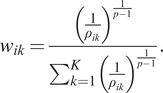 $$ {w}_{ik}=\frac{{\left(\frac{1}{\rho_{ik}}\right)}^{\frac{1}{p-1}}}{\sum_{k=1}^K{\left(\frac{1}{\rho_{ik}}\right)}^{\frac{1}{p-1}}}. $$
IDW assumes that the nearby values contribute more to the interpolated values than distant observations. In this way the influence of a known data point is inversely related to the distance from the unknown location that is being estimated. Thus defined, $ {w}_{ik} $
can take any real value between 0 and 1. This is the continuous nature of CIGSCR. Every data point belongs to every cluster with some probability, also known as fuzzy clustering. The updated cluster means are then calculated as
$ {w}_{ik} $
can take any real value between 0 and 1. This is the continuous nature of CIGSCR. Every data point belongs to every cluster with some probability, also known as fuzzy clustering. The updated cluster means are then calculated as
 $$ {\mu}_k=\frac{1}{\sum_{i=1}^N{w}_{ik}^p}\sum \limits_{i=1}^N{w}_{ik}^p{x}^i. $$
Let $ c={c}_1,\dots, {c}_C $
denote the aspired phases that need to be extracted. The null hypothesis is formulated as “the mean weight of
$ c={c}_1,\dots, {c}_C $
denote the aspired phases that need to be extracted. The null hypothesis is formulated as “the mean weight of $ c $
th phase in
$ c $
th phase in $ k $
th cluster is not significantly different from the mean weights for all the phases present in the sample.” The alternate hypothesis is that the average cluster weights corresponding to
$ k $
th cluster is not significantly different from the mean weights for all the phases present in the sample.” The alternate hypothesis is that the average cluster weights corresponding to $ c $
th class are significantly different from the average cluster weights corresponding to all classes. Alternate hypothesis holding true then indicates that the cluster statistically comprises a single phase. Let
$ c $
th class are significantly different from the average cluster weights corresponding to all classes. Alternate hypothesis holding true then indicates that the cluster statistically comprises a single phase. Let $ \hat{z} $
denote a test statistic, and
$ \hat{z} $
denote a test statistic, and $ \alpha $
denote the user-defined threshold for statistical significance. Then, for any cluster,
$ \alpha $
denote the user-defined threshold for statistical significance. Then, for any cluster, $ P\left(\hat{z}<Z\right)>\alpha $
implies that the mean weight of
$ P\left(\hat{z}<Z\right)>\alpha $
implies that the mean weight of $ c $
th class in
$ c $
th class in $ k $
th cluster is not significantly different from that of other classes. Such a cluster is rejected. This cluster is split into two clusters: one comprising the dominant class and a second comprising the remaining classes. The mean weights are estimated using the training data and the weights
$ k $
th cluster is not significantly different from that of other classes. Such a cluster is rejected. This cluster is split into two clusters: one comprising the dominant class and a second comprising the remaining classes. The mean weights are estimated using the training data and the weights $ {w}_{ik} $
. Association significance test (Wald test statistic) is used to estimate statistical purity. For independent and identically distributed data, Wald test statistic is
$ {w}_{ik} $
. Association significance test (Wald test statistic) is used to estimate statistical purity. For independent and identically distributed data, Wald test statistic is
 $$ \hat{z}=\frac{n_c\left({\overline{w}}_{ik}-{\overline{w}}_k\right)}{s_k}, $$
where $ {\overline{w}}_k $
denotes the average weight of all classes in
$ {\overline{w}}_k $
denotes the average weight of all classes in $ k $
th cluster,
$ k $
th cluster, $ {\overline{w}}_{ik} $
denotes the average weight of class
$ {\overline{w}}_{ik} $
denotes the average weight of class $ c $
in the
$ c $
in the $ k $
th cluster,
$ k $
th cluster, $ {s}_k $
is the sample standard deviation of
$ {s}_k $
is the sample standard deviation of $ k $
th cluster, and
$ k $
th cluster, and $ {n}_c $
is the cardinality of the training data for class
$ {n}_c $
is the cardinality of the training data for class $ c $
. The composition of a rock sample is inherently characterized by various phases being present in varying proportions (and not in an identically distributed manner). With the same reasoning as provided in Phillips et al. (Reference Phillips, Watson and Wynne2011), the test statistic used is, therefore,
$ c $
. The composition of a rock sample is inherently characterized by various phases being present in varying proportions (and not in an identically distributed manner). With the same reasoning as provided in Phillips et al. (Reference Phillips, Watson and Wynne2011), the test statistic used is, therefore,
 $$ \hat{z}=\frac{y_{ck}-{n}_c{\overline{w}}_k}{\sqrt{p_c{\sum}_d{n}_d\left({S}_{wj}^2+\left(1-{p}_c\right){w}_{dj}^2\right)}}, $$
where $ {y}_{ck} $
is the sum of cluster weights for voxels labeled with
$ {y}_{ck} $
is the sum of cluster weights for voxels labeled with $ c $
-th phase to the
$ c $
-th phase to the $ k $
-th cluster and
$ k $
-th cluster and $ {p}_c $
is a maximum likelihood estimate of the prior for classification of phase
$ {p}_c $
is a maximum likelihood estimate of the prior for classification of phase $ c $
as determined by the training data. A negative value of test statistic is taken as an indication that the current cluster has a phase that is not represented at all in the existing set of phases (labeled data). A new phase is then added to the training dataset from such a cluster if such addition yields a positive test statistic for this cluster. This is done by choosing from any slice, a physically contiguous sample of three voxels from the direction of least variation (in grayscale values) with a randomly selected pixel from the negative cluster as a pivot. For the new cluster created as a result of cluster splitting, the cluster mean is calculated as
$ c $
as determined by the training data. A negative value of test statistic is taken as an indication that the current cluster has a phase that is not represented at all in the existing set of phases (labeled data). A new phase is then added to the training dataset from such a cluster if such addition yields a positive test statistic for this cluster. This is done by choosing from any slice, a physically contiguous sample of three voxels from the direction of least variation (in grayscale values) with a randomly selected pixel from the negative cluster as a pivot. For the new cluster created as a result of cluster splitting, the cluster mean is calculated as
 $$ {\mu}_{new}=\frac{\sum_{i\in {\Phi}^{-1}\left({c}_k\right)}{w}_{ik}{x}_i}{\sum_{i\in {\Phi}^{-1}\left({c}_k\right)}{w}_{ik}}, $$
where $ k $
is the cluster with lowest value of
$ k $
is the cluster with lowest value of $ \hat{z} $
,
$ \hat{z} $
, $ {c}_k $
denotes the majority class of the
$ {c}_k $
denotes the majority class of the $ k $
th cluster,
$ k $
th cluster, $ {\Phi}^{-1} $
denotes the training dataset,
$ {\Phi}^{-1} $
denotes the training dataset, $ {\Phi}^{-1}(c) $
denotes the samples provided for phase
$ {\Phi}^{-1}(c) $
denotes the samples provided for phase $ c $
in the training dataset. Once the updated cluster means are available, optimization problem (equation 3) is solved again with the updated set of clusters. The algorithm iterates until either a maximum number of iterations are reached, or each identified cluster reaches a minimum homogeneity level.
$ c $
in the training dataset. Once the updated cluster means are available, optimization problem (equation 3) is solved again with the updated set of clusters. The algorithm iterates until either a maximum number of iterations are reached, or each identified cluster reaches a minimum homogeneity level.
When the iterative loop ends, the membership value of each voxel toward each cluster is observed. Let $ K $
now denote the total number of clusters at this point. Let
$ K $
now denote the total number of clusters at this point. Let $ p\left({k}_j|x\right) $
denote the probability of voxel
$ p\left({k}_j|x\right) $
denote the probability of voxel $ x $
belonging to cluster
$ x $
belonging to cluster $ {k}_j $
; this can be estimated using
$ {k}_j $
; this can be estimated using $ {w}_{ik} $
. For a voxel
$ {w}_{ik} $
. For a voxel $ x $
, if there exists
$ x $
, if there exists $ 1\le \hskip2pt {j}^{\ast}\le \hskip2pt K $
such that
$ 1\le \hskip2pt {j}^{\ast}\le \hskip2pt K $
such that $ p\left({k}_{j^{\ast }}|x\right)>\tau $
, then that voxel is assigned to cluster
$ p\left({k}_{j^{\ast }}|x\right)>\tau $
, then that voxel is assigned to cluster $ {k}_{j^{\ast }} $
. For all
$ {k}_{j^{\ast }} $
. For all $ j\in 1,\dots, K,\hskip2pt j\ne {j}^{\ast } $
,
$ j\in 1,\dots, K,\hskip2pt j\ne {j}^{\ast } $
, $ p\left({k}_j|x\right) $
is set to zero.
$ p\left({k}_j|x\right) $
is set to zero. $ \tau \in \left(0,1\right) $
, here, is a user-defined parameter. On the other hand, if
$ \tau \in \left(0,1\right) $
, here, is a user-defined parameter. On the other hand, if $ p\left({k}_j|x\right)<\tau \hskip2pt \forall \hskip2pt j\in 1,\dots, K $
, then the voxel exhibits significantly high membership values toward at least two clusters. Such voxels are assigned a distinct cluster, say,
$ p\left({k}_j|x\right)<\tau \hskip2pt \forall \hskip2pt j\in 1,\dots, K $
, then the voxel exhibits significantly high membership values toward at least two clusters. Such voxels are assigned a distinct cluster, say, $ {\mu}_{K+1} $
. The source of this “uncertainty” could be factors such as the voxel falling on the boundary of two physical phases.
$ {\mu}_{K+1} $
. The source of this “uncertainty” could be factors such as the voxel falling on the boundary of two physical phases. $ \tau =0.86 $
was used for all the experiments carried out in this study. The overall complexity of the algorithm is
$ \tau =0.86 $
was used for all the experiments carried out in this study. The overall complexity of the algorithm is $ \mathcal{O}(NK), $
assuming
$ \mathcal{O}(NK), $
assuming $ N>>K. $
Finally, classification is carried out to decide/assign physical meaning to each cluster. Let $ p\left({c}_i|x\right) $
denote the probability that voxel
$ p\left({c}_i|x\right) $
denote the probability that voxel $ x $
belongs to phase
$ x $
belongs to phase $ {c}_i $
. Then
$ {c}_i $
. Then
 $$ p\left({c}_i|x\right)=\sum \limits_{j=1}^{K+1}p\left({c}_i,{k}_j|x\right)p\left({k}_j|x\right)=\sum \limits_{j=1}^{K+1}p\left({c}_i|{k}_j,x\right)p\left({k}_j|x\right). $$
Suppose the user assigns cluster $ {k}_j $
to class
$ {k}_j $
to class $ {c}_i. $
Also, let
$ {c}_i. $
Also, let $ {c}_{C+1} $
be a new phase that will comprise voxels of “unknown” class such as those lying on the interface of two phases. The classification function
$ {c}_{C+1} $
be a new phase that will comprise voxels of “unknown” class such as those lying on the interface of two phases. The classification function $ p\left({c}_i|x\right) $
defined as
$ p\left({c}_i|x\right) $
defined as
 $$ {\displaystyle \begin{array}{c} Class(x)=\arg {\max}_{1\le i\le C+1}p\left({c}_i|x\right)\\ {}=\arg {\max}_{1\le i\le C+1}\sum p\left({c}_i|{k}_j,x\right)p\left({k}_j|x\right)\end{array}} $$
where $ p\left({k}_j|x\right) $
can be calculated using the weight matrix, and
$ p\left({k}_j|x\right) $
can be calculated using the weight matrix, and
 $$ p\left({c}_i|{k}_j,x\right)=\left\{\begin{array}{ll}1& \mathrm{if}\;{k}_j\hskip0.5em \mathrm{is}\ \mathrm{labeled}\hskip0.5em {c}_i\\ {}0& \mathrm{otherwise}\end{array}\right.. $$
This produces the final segmentation. The voxels that get left as “unclassified” in the end are a subset of voxels in the $ \left(K+1\right) $
th cluster.
$ \left(K+1\right) $
th cluster.
Throughout this work, the term “cluster” is used to refer to the “grayscale intensity bins” obtained using CIGSCR. The terms “phase” and “class” are used interchangeably to denote a physically meaningful entity such as “quartz” or “pore” or “clay” or “feldspar.” For any given geological formation, multiple “samples” are collected for analysis. Each sample is imaged usually at more than one sub-regions. The image acquired for one subregion of a sample is referred to as “scan” or “miniplug.” The terms “scan” and miniplug are used interchangeably.
4. Input Data
Micro-CT scans of rock samples meant for DRP are used in this paper. Experiments were carried out on a wide variety of rock samples (more than 100 unique samples, full as well as various subvolumes from those samples) from various geographical sources. One lab, two outcrops, and one reservoir rock sample are presented in this paper as representative examples. The samples were chosen span a range of grain size (0.05-0.5 mm) and porosity (5%–20%) values. This section describes these selected samples.
-
• Glassbeads (GB): This is a lab-generated sample. Glass beads are encased in epoxy resin and scanned. Theoretically, the beads are of uniform composition. However, some density variance is observed in micro-CT images. For segmentation, a binary segmentation comprising pore and mineral is the desired outcome. Effects of beam hardening, sample CT density variance, and edge effects from raw projection reconstruction need to be dealt with efficiently. The sample used in this study is acquired at 2.05 μm.
-
• Fontainebleau sandstone (FB33): Oligocene age Fontainebleau sandstone is a moderately well-sorted, sub-rounded to rounded, and well-cemented (20%) sandstone. Cement precipitation during dissolution compaction as well as subsequent secondary processes has resulted in an abundance of quartz cement. Due to such significant cementation as well as other reasons, these samples have low porosity $ \left(<\hskip-2pt 10\%\right). $
These samples are categorized as quartzarenite; compositionally, these are almost pure quartz with minimal rock fragments and feldspars present. Fontainebleau sandstones are well studied with a considerable amount of laboratory measurements, including sonic velocities, permeability, and electrical properties. The Fontainebleau sample used in this study is acquired at 0.99um.
$ \left(<\hskip-2pt 10\%\right). $
These samples are categorized as quartzarenite; compositionally, these are almost pure quartz with minimal rock fragments and feldspars present. Fontainebleau sandstones are well studied with a considerable amount of laboratory measurements, including sonic velocities, permeability, and electrical properties. The Fontainebleau sample used in this study is acquired at 0.99um. -
• Castlegate sandstone (CG): The Castlegate Formation of Utah is a moderately sorted, subangular to sub-rounded Mesozoic sandstone with a mean grain size of 200 mm. X-ray diffraction (XRD) analysis indicates that the Castlegate sandstone sample consists mainly of quartz grains. Petrologic assessment indicates a minimal quartz cement volume (2–3%), similar amounts of carbonate cement, and minor amounts of clay minerals, including kaolinite, muscovite, and smectite-illite. In quartz-feldspar-rock fragment space, commonly used to categorize rocks by their constituents, the Castlegate is a feldspathic litharenite with the rock fragments dominantly being altered and unaltered volcanic rock fragments. It is within these rock fragments that most of the clays reside. On the basis of manual point counting, the total macroporosity in CG is 19% (or pu: porosity unit). The Castlegate sample used here is acquired at 2.05 μm resolution.
-
• Reservoir Rock: An actual reservoir rock is considered. This sample is selected for analysis due to its mineralogical complexity, where quartz, K-feldspar, plagioclase, calcite, dolomite, siderite, barite, halite, pyrite, anatase, undifferentiated illite plus mixed-layer illite/smectite, muscovite, kaolinite and chlorite are all present and manifest in micro-CT images as a range of grayscales. The texture and mineralogy of this rock still fall within the operatign envelope of Digital Rock (DR; Saxena et al., Reference Saxena, Hows, Hoffmann, Alpak, Freeman, Hunter and Appel2018). The porosity of this rock is around 20%, the grains are subangular, and moderately sorted. The sample used in this paper is imaged at 1.54 μm resolution.

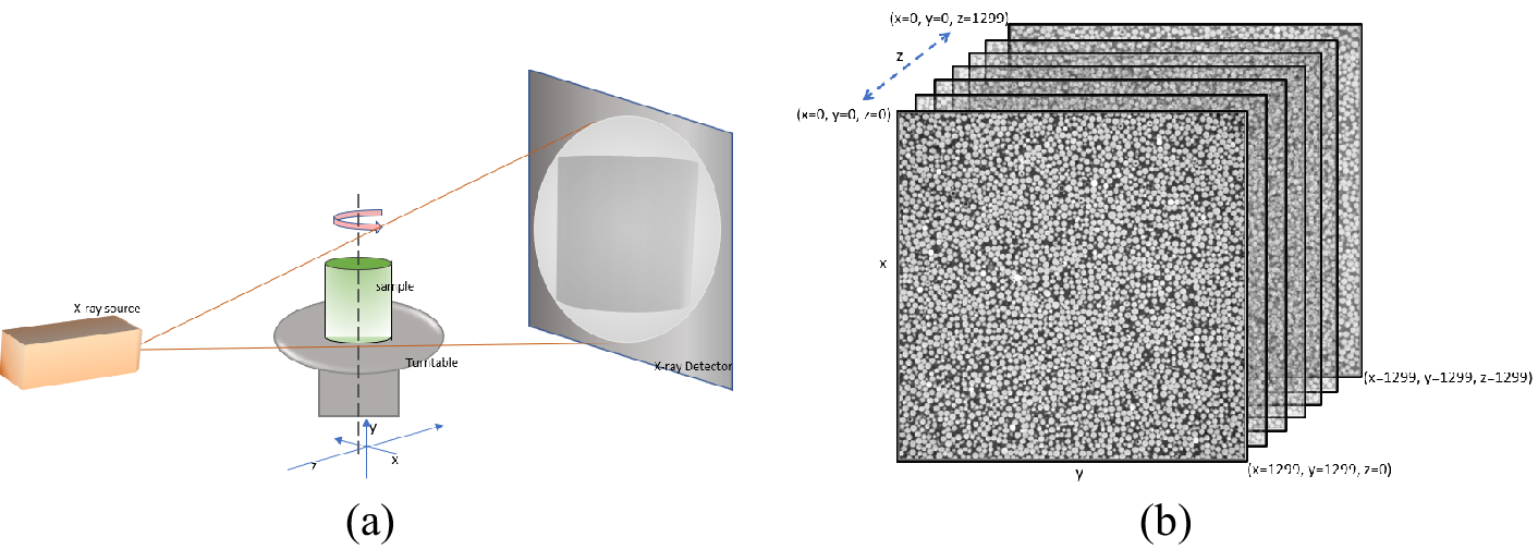
The input samples presented in this paper are acquired using a laboratory-based micro-CT scanner (Figure 1). An X-ray tube with a cone beam irradiation system and a flat panel CCD detector is housed in a radiation shield instrument. Each sample is a 5mm miniplug, cylindrical in shape, placed on a rotating table in between the X-ray source and the detector. The raw data thus collected comprises radon-transformed values. Zeiss software distributed with the machine is used to reconstruct physical 3D images from the raw data. 16-bit images are generated (meaning, the grayscale values range from 0 to 65535). The reconstructed images are filtered (to reduce noise) using an in-house nonlocal means filter with a parameter of 0.75. The $ {1300}^3 $
cube at the center of the filtered micro-CT image is retained for analysis (Figure 1(b)).
$ {1300}^3 $
cube at the center of the filtered micro-CT image is retained for analysis (Figure 1(b)).
(a) Cone beam micro-CT setup for data acquisition, (b) input micro-CT image for CIGSCR.
The resolution chosen for imaging the rock samples has a significant impact on the estimates of rock properties computed using DR technology. The effect of voxel size chosen for imaging the rock samples is discussed in Saxena et al. (Reference Saxena, Hoffmann, Alpak, Dietderich, Hunter and Day-Stirrat2017). In general, 2um is found to be an optimal image resolution, providing a good tradeoff between the field of view and accuracy of subsequent physical measurements. The exact resolution used for any given sample may vary from 0.5 μm to 4 μm. A segmentation algorithm needs to operate in a consistent and stable manner across this practice resolution range. Current micro-CT detectors are not able to image finer than 1 μm; analyzing 3D images of smaller voxel sizes is thus not possible.
5. Results
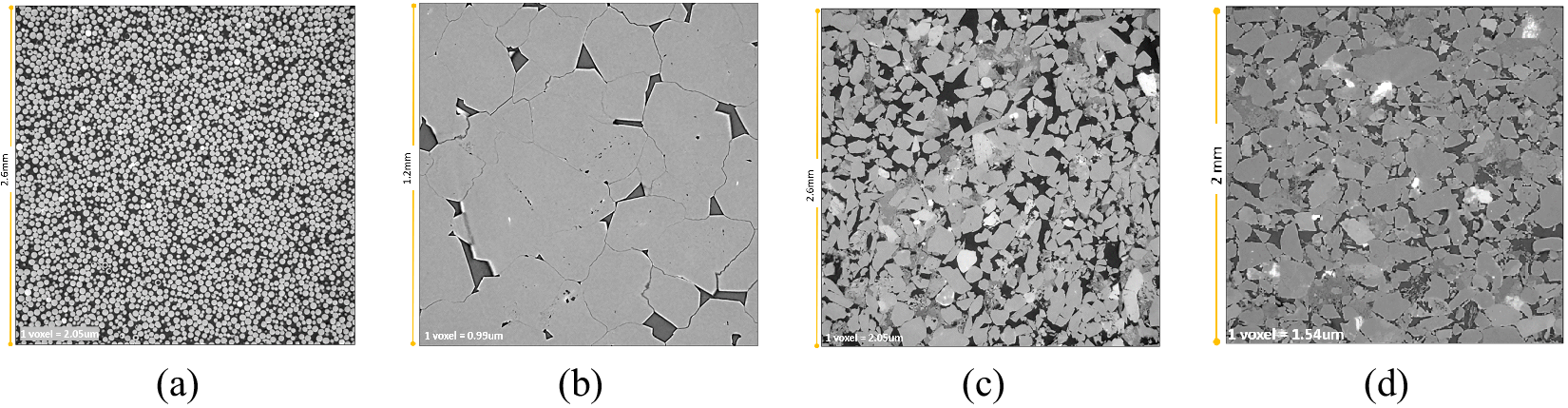
The center slices of the four scans (four samples) described in Section 4 are displayed in Figure 2, and their grayscale intensity histograms are in Figure 3. The histograms in Figure 3 have been zoomed in and the x-limits adjusted (clipped) to display only the range in which the bulk of the gray values fall. While the actual distribution varies from sample to sample, the grayscale histogram for each volume has two distinct peaks––the lower grayscale value peak that corresponds to pore space and the higher grayscale value peak that corresponds to quartz. The histograms are easily seen to be Gaussian mixtures. Porous minerals, hydrocarbons, and other low-density materials occupy the intensity values in between the two significant peaks while the denser rock grains fall to the right of the quartz peak on the histogram. When minerals with high attenuation coefficients are present (e.g., pyrites), the intensity values of multiple lower-density minerals such as quartz and feldspar with similar attenuation coefficients get compressed into a rather narrow grayscale range (e.g., Figure 3a,b vs. c,d).
Input image center slices. (a) Glass beads, (b) Fontainebleau sandstone ( $ <\hskip-2pt 10\% $
porosity), (c) Castlegate sandstone (
$ <\hskip-2pt 10\% $
porosity), (c) Castlegate sandstone ( $ <\hskip-2pt 19\% $
porosity), and (d) Reservoir rock (
$ <\hskip-2pt 19\% $
porosity), and (d) Reservoir rock ( $ \approx 20\% $
porosity).
$ \approx 20\% $
porosity).
Input image histograms. (a) Glass beads, (b) Fontainebleau, (c) Castlegate sandstone, and (d) Reservoir rock.

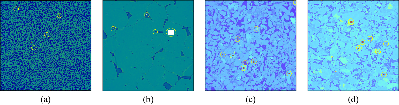
Training data for each input volume is provided by selecting a few pixels from each phase of interest. So, for a fixed phase, the training data could be a rectangular patch (selected by click-and-drag) or a sequence of pixels (selected by clicking on individual pixels). In this study, the training data is provided only from the center slice of the respective image volume. Training data overlaid on the center slice of each sample is displayed in Figure 4. The circled rectangles overlaid on each image depict the specific training data that was provided for respective phases. A total of 236, 6587, 2697, and 1545 voxels were provided as training data for Glassbeads, Fontainebleau, Castlegate, and Reservoir rock samples, respectively.
Training data. (a) Glass beads, (b) Fontainebleau, (c) Castlegate sandstone, and (d) Reservoir rock.
Validation is mainly based on visual assessment of pixelwise accuracy, with a close focus on microstructures. Porosity and permeability are presented as probabilistic bounds, rather than absolute/dot values. Porosity, in particular, is matched with the results from another algorithm (SFCM) as well as laboratory measurements, when available. Rest of the mineralogy is calculated and presented but not compared with any benchmark. All quantitative estimates are viewed keeping in mind that digital images have finite resolution and that spectral clustering in itself has known limitations that are outside the scope of this initial step toward semisupervised segmentation.
The proposed clustering algorithm was run for 15, 23, 30, and 30 iterations, respectively. The outcomes after this number of iterations for each sample are shown in Figure 5. The number of iterations (equal to the number of clusters) to be used is determined based on the complexity (assessed visually) of the sample. In general, due to the imaging artifacts, 15 to 30 clusters are found useful. For “simpler” samples (large grains, only a few phases, such as that in Glassbeads and Fontainebleau), 15 and 23 iterations are used here. Castlegate and the Reservoir rock are complex samples (highly heterogeneous in composition, small grains with complex, varying shapes) that provide a representative view of real-world samples. For such samples, more iterations are needed; this work uses 30 iterations for Castlegate and Reservoir rock.
Clusters attained. (a) Glass beads (synthetic, 15 iterations), (b) Fontainebleau (23 iterations), (c) Castlegate sandstone (30 iterations), (d) Reservoir rock (30 iterations). Notice the artificial phase named “unresolved” used while grouping clusters for each sample.
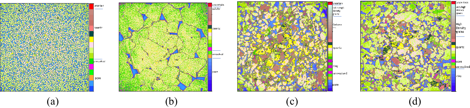
Fidelity of the clusters with the training data provided (by the user) for quartz and pore phases is used to calibrate the color code for displaying the clustering outcome for each sample. For each sample, the various intensities corresponding to pore space are displayed in different shades of blue. Pink corresponds to the grayscale intensities that appeared in the rectangular patch that was provided as labeled data for quartz. The different grayscale intensities appearing in between quartz and pore (e.g., clay) are displayed in brown, different shades of green, and magenta. Quartz, again, exhibits at least two intensity clusters––one that is displayed in pink and forms the bulk of quartz grains, and a second that is displayed in yellow. Notice that, for each of the five samples, CIGSCR produces a distinct lower-intensity cluster toward the periphery of the image volumes (depicted in darker shades of green in the images in Figure 5). This lower intensity cluster results from the fact that micro-CT images in DR are characterized by variation in grayscale so that a grain or pore space at the center of an image volume exhibits a different grayscale intensity range than the same mineral or pore at the edge of the volume. This phenomenon is known as “cupping effect” (Boas and Fleischmann, Reference Boas and Fleischmann2012; Hunter and McDavid, Reference Hunter and McDavid2012; Jovanovic et al., Reference Jovanovic, Khan, Enzmann and Kersten2013), a combined outcome of two underlying phenomena: beam hardening and scatter radiation. The variation is typically radial nonlinear (grayscale values increase toward the edges), may not always be visible to the human eye, and its expanse varies from sample to sample. Cupping effect hampers the performance of most segmentation/feature extraction algorithms. CIGSCR alleviates the impact of cupping effects on feature extraction significantly by allowing the user to generate excess clusters that can be appropriately treated during postprocessed. Red color voxels in each sample depict uncertain voxels.
The clusters displayed in Figure 5 are postprocessed as described in equation 11. The grouping of clusters is determined by the user based on the physically meaningful phases that are of interest to them. In addition to the $ K $
clusters and
$ K $
clusters and $ C $
phases discussed in Section 3, one to two clusters that lie at the boundary of pore and nonpore (clay or solid phase) gray values is assigned to a phase named “unresolved.” “Unresolved” is a synthetic phase that is introduced in order to account for uncertainties that the discrete nature of digital image acquisition/processing incurs. This phase represents partial voxels that lie at the interface of pore–grain interface. For any given input, therefore, the final segmentation comprises
$ C $
phases discussed in Section 3, one to two clusters that lie at the boundary of pore and nonpore (clay or solid phase) gray values is assigned to a phase named “unresolved.” “Unresolved” is a synthetic phase that is introduced in order to account for uncertainties that the discrete nature of digital image acquisition/processing incurs. This phase represents partial voxels that lie at the interface of pore–grain interface. For any given input, therefore, the final segmentation comprises $ C $
physically meaningful phases, one artificial phase named “unresolved,” and one phase comprising “unclassified” voxels (equation 11). Note that “unclassified” voxels are different from “unresolved” voxels––the former denotes an algorithmic limitation (see Section 3) while “unresolved” refers to a machine/digitalization limitation and captures the set of voxels at the pore–grain boundary and depicts voxels that ended up getting a gray value matching that of a true physical phase (clay/porous mineral).
$ C $
physically meaningful phases, one artificial phase named “unresolved,” and one phase comprising “unclassified” voxels (equation 11). Note that “unclassified” voxels are different from “unresolved” voxels––the former denotes an algorithmic limitation (see Section 3) while “unresolved” refers to a machine/digitalization limitation and captures the set of voxels at the pore–grain boundary and depicts voxels that ended up getting a gray value matching that of a true physical phase (clay/porous mineral).
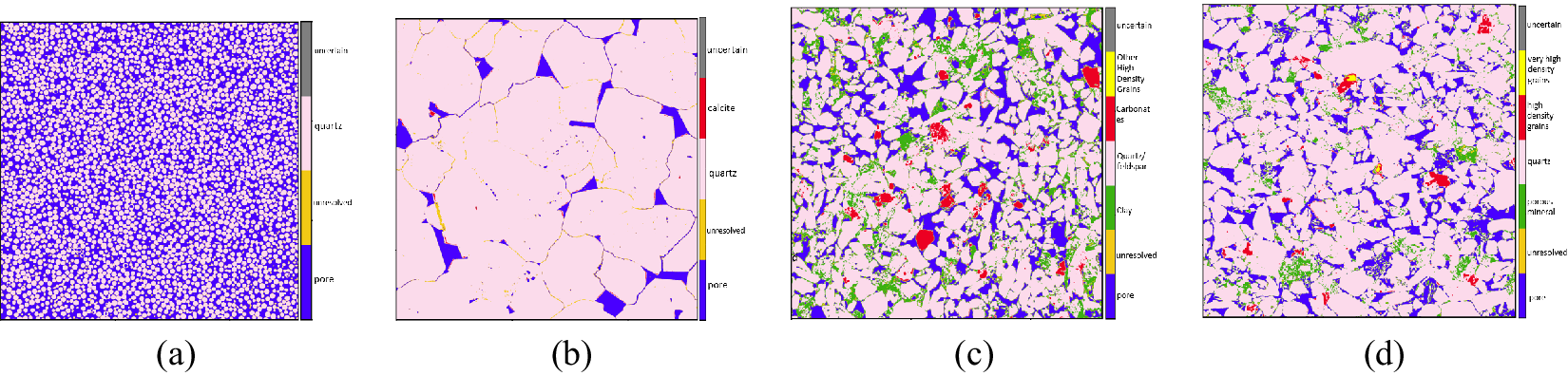
Guided by such grouping, one possible set of combinations for the study samples is displayed in Figure 5 alongside the respective images. Segmentations attained using listed groupings are displayed in Figure 6. For Glassbeads, the clusters are grouped to produce a two-phase segmentation: pore space and solid. For the Fontainebleau sample, the clusters are combined to retain three phases––pore, quartz, and calcite. For Castlegate, the 30 clusters are grouped to extract a five-phase segmentation as shown in Figure 6c. For the Reservoir Rock, a five-phase segmentation is extracted: pore, clay aggregate, quartz (including feldspar), and two strata of high-density materials (high and very high). The gray color in the colorbar of each sample corresponds to unclassified voxels (equation 11) and the dark yellow phase (just above “pore”) corresponds to the unresolved voxels.
Segmented images. (a) Glass beads (two-phases), (b) Fontainebleau (three-phase), (c) Castlegate (five-phase), and (d) Reservoir rock (five-phase).
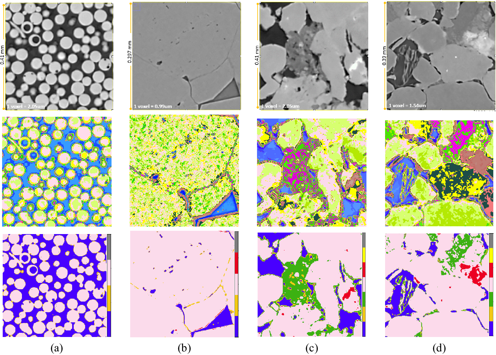
For each sample, one zoomed-in 2D section with representative complexity/challenges from the center slice is displayed in Figure 7 (top row). The clusters obtained for this zoomed-in portion are displayed in the middle row, and the segmentation for respective zoomed-in portions displayed in Figure 7 (bottom row). For the Glassbeads sample, three to four types of intensities appear interesting in the grayscale image: beads (note the edge effects), light beads (not captured in the zoomed-in window here), two grayscales in the pore space, and two clay grayscales for bead slightly out of plane. Clusters for each of these phases are extracted. In the final segmentation (bottom row), two phases are retained; notice that the out-of-plane phases and the broken beads are correctly classified. For Fontaineblueau, five intensities seen as interesting: quartz (note edge effects), 3 grayscales in the pore space, and grain-grain interface grayscales. In the three-phase segmentation finally retained, the grain-grain contact surfaces and grain-pore boundary voxels are assigned unresolved labels. Unresolved voxels closely line the pore–grain boundaries. For Castlegate and Reservoir rock samples the pore–grain interface lining is marked with both clay voxels (misclassified) and unresolved voxels and the unresolved phase provides a close approximation to the pore–grain interface voxels that are mislabeled as clay/porous mineral.
Zoomed in grayscale and segmented regions. (a) Glass beads, (b) Fontainebleau, (c) Castlegate sandstone, and (d) Reservoir rock.
The percentage of voxels for each phase is calculated for each sample. Empty/pore voxels and porous mineral voxels are two primary phase fractions in analyzing rock samples. The synthetic phase “unresolved” facilitates reporting porosity with probabilistic bounds. Specifically, if $ E $
is the number of confident pore (empty) voxels,
$ E $
is the number of confident pore (empty) voxels, $ U $
the number of unresolved voxels, and
$ U $
the number of unresolved voxels, and $ P $
the number of porous mineral voxels, the estimate on pore voxels is provided as
$ P $
the number of porous mineral voxels, the estimate on pore voxels is provided as $ {E}_{est}=\left(E,E+U\right) $
, and the estimate on porous mineral is provided as
$ {E}_{est}=\left(E,E+U\right) $
, and the estimate on porous mineral is provided as $ {P}_{est}=\left(P-U,P\right) $
. For Glassbeads, pore voxels are estimated to be in the range (43–49%), and the solid phase is (50.8–56.5%). For Fontainebleau, pore voxels are estimated to be in between (4.67–6.01%), quartz in range (93.8–95.2%), and high-density mineral is less than 0.12%. For Castlegate, estimates are pore voxels (15%,18.7%), porous mineral voxels (8.5%,12.3%), quartz 67%, and bright minerals 0.004%. For the reservoir rock, volumetric estimates stand at pore voxels (14.6%,16.5%), porous mineral voxels (4.25%,6.2%), quartz is 75.8%, carbonates is 1.44%, and very high-density minerals 0.002% (traces). Unclassified voxels at the end of classification are Glassbeads 0.02%, Fontainebleau 0.075%, Castlegate 0.2%, and Reservoir rock 0.2%. On being multiplied by appropriate rock-dependent constants, the values of porosity, permeability, and other volumetrics are obtained. SFCM (Chuang et al., Reference Chuang, Tzeng, Chen, Wu and Chen2006) (see Section 2), implemented to give probabilistic bounds on porosity (a lower and an upper limit), estimates of porosity for Glassbeads sample are in between 41% and 49%, Fontainebleau between 4.85 and 5.58%, for the Castlegate sample between 17.33 and 21.60%, and for the reservoir rock between 14.43 and 17.54%.
$ {P}_{est}=\left(P-U,P\right) $
. For Glassbeads, pore voxels are estimated to be in the range (43–49%), and the solid phase is (50.8–56.5%). For Fontainebleau, pore voxels are estimated to be in between (4.67–6.01%), quartz in range (93.8–95.2%), and high-density mineral is less than 0.12%. For Castlegate, estimates are pore voxels (15%,18.7%), porous mineral voxels (8.5%,12.3%), quartz 67%, and bright minerals 0.004%. For the reservoir rock, volumetric estimates stand at pore voxels (14.6%,16.5%), porous mineral voxels (4.25%,6.2%), quartz is 75.8%, carbonates is 1.44%, and very high-density minerals 0.002% (traces). Unclassified voxels at the end of classification are Glassbeads 0.02%, Fontainebleau 0.075%, Castlegate 0.2%, and Reservoir rock 0.2%. On being multiplied by appropriate rock-dependent constants, the values of porosity, permeability, and other volumetrics are obtained. SFCM (Chuang et al., Reference Chuang, Tzeng, Chen, Wu and Chen2006) (see Section 2), implemented to give probabilistic bounds on porosity (a lower and an upper limit), estimates of porosity for Glassbeads sample are in between 41% and 49%, Fontainebleau between 4.85 and 5.58%, for the Castlegate sample between 17.33 and 21.60%, and for the reservoir rock between 14.43 and 17.54%.
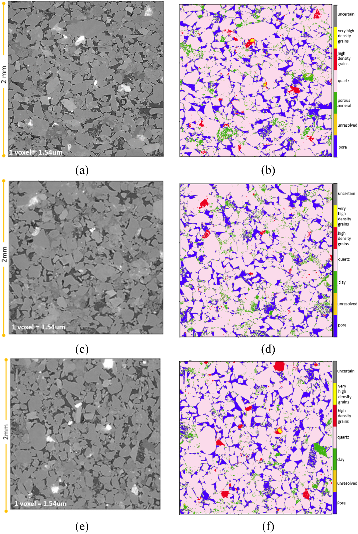
Once again, by design, the approach is inherently applicable to three-dimensional data. Figure 8 displays cross-sections of the input volume and the final segmented volume along the center slices in each of the three directions for the reservoir rock. As mentioned earlier, the input training data was provided only from the XY-slice (Figure 8). Segmentation along YZ- and XZ-directions is achieved with similar accuracy.
Center slices of reservoir rock for each of the three axes: (a,b) XY slice (z = 649); (c,d) YZ slice (x = 649), (e,f) XZ slice (y = 649).
6. Discussions
The primary technical strengths of the proposed approach include (i) the need for very little training data, (ii) the ability to capture heterogeneity within individual phases, (iii) limited sensitivity to threshold value, (iv) robustness against histogram translations and compressions, and (v) the fact that the approach is semi-supervised and requires limited user inputs. Another strength is seen in CIGSCR’s ability to handle cupping effects.
CIGSCR does not offer end-to-end segmentation. CIGSCR, instead, splits the histogram down into intensity clusters. This splitting provides the foundation for classification strategies that can be implemented as postprocessing operations to get the final segmentation. In general, CIGSCR has the ability to locate clusters associated with classes, even when there is an overlap between classes. For GB2 (Figure 7a), with 15 iterations for clustering, two clusters are attained in the pore space. These reflect the variance in the grayscale in pore space––one for the bulk of the pore space, and the second for the grayscale dip that is observed at grain–pore interface. Such splitting of grayscale intensities enables determining the segmentation strategy that can be applied to the volume. Similar splitting of clusters helps overcome beam hardening whenever it is present in a sample. In addition, in the event that a rock sample had liquids with varying densities in pore space, this splitting can be used to segment pore-filling liquids/fluids. For GB2, all intensity clusters for pore space are combined back into a single phase, similarly for beads, and similarly for beam hardening corrections in all samples. In case of heterogeneous grains such as Feldspar, the heterogeneity as such is captured and is visible in the clustermaps. However, isolating feldspar grains distinctly from quartz in the final classification requires a more sophisticated postprocessing/classification strategy.
The accuracy of final segmentation in terms of resolving pore–grain artifacts increases as the number of iterations is increased. The increased number of iterations also facilitates securing one to two clusters as “unresolved” voxels. For simpler samples such as Glassbeads and Fontainebleau, this phase directly represents partial voxels at pore–grain boundary. For more complex samples such as Castlegate and Reservoir rock, the final segmentation exhibits a clay lining all along the pore–grain interface (see Figure 7c), and is closely accompanied by the “unresolved” voxels. These clay voxels, in reality, are either partial voxels (part pore, part solid) or interface reconstruction artifacts. Emerging methods such as Weka and Ilastik display/label these boundary voxels (both false-clay and unresolved united) as “unresolved” voxels; for CIGSCR similar output could be achieved by using spatial correlation between clay voxels and unresolved voxels but such a step is not included here to avoid information loss.
All segmentation approaches can perform poorly when training data is insufficient (samples within the dataset are not represented in the training set). Figure 9 illustrates that CIGSCR copes reasonably stably with such unseen data. Figure 9a displays the histogram for the center slice of this volume. For this sample, nine phases were provided as training data from this slice. Figure 9b displays the histogram for the entire volume. The grayscale range (approximately, 1,100–21,000) for the center slice is clearly much smaller than the grayscale range (0 to approximately 65,000) for the full volume, indicating that the center slice does not contain all the minerals/phases present in the full volume. Thirty clusters were generated for this sample. Figure 9c displays the top-left quadrant ( $ 500\times 500 $
) of slice 1000 of the input volume. A careful look at this slice reveals the presence of high-density grains (marked with the red arrow in Figure 9c). Figure 9d displays the corresponding portion of slice 1000 from the segmented volume. Note that, one, the high-density grains have grayscale variance not distinguishable with the bare eye. CIGSCR has segmented them into separate phases. Second, the composition of rock samples varies from one geological formation to another, as well as across multiple samples taken from a given geological formation. To add to that, the input samples used in DR workflow are 3D volumes. Whichever slice the user uses for providing the training data, there can always be other slices containing minerals that are not present in the slices that the user looked at. Given such unpredictability in prior knowledge, automatic detection of phases is a critical attribute of a segmentation algorithm for these 3D volumes.
$ 500\times 500 $
) of slice 1000 of the input volume. A careful look at this slice reveals the presence of high-density grains (marked with the red arrow in Figure 9c). Figure 9d displays the corresponding portion of slice 1000 from the segmented volume. Note that, one, the high-density grains have grayscale variance not distinguishable with the bare eye. CIGSCR has segmented them into separate phases. Second, the composition of rock samples varies from one geological formation to another, as well as across multiple samples taken from a given geological formation. To add to that, the input samples used in DR workflow are 3D volumes. Whichever slice the user uses for providing the training data, there can always be other slices containing minerals that are not present in the slices that the user looked at. Given such unpredictability in prior knowledge, automatic detection of phases is a critical attribute of a segmentation algorithm for these 3D volumes.
Minerals not present in training set: Castlegate sample (a) Slice 650 (the center slice) where the training data was collected from; (b,c) histograms for slices 650 and the full micro CT volume, respectively. The full volume has high-density grains that are not present in the center slice; (d) slice 1,000 of the input, first quadrant. This region has a halite that was not present in the center slice and, therefore, not included in the training data; (e) CIGSCR-based segmentation resulting for this slice/region. Same grouping of clusters is used as that in Figure 5.

Figure 10 focuses on the Castlegate sample to demonstrate (i) the multiphase segmentation attribute of CIGSCR, and (ii) that once a reasonable number of clusters has been obtained (the somewhat time-taking step), those clusters can be grouped in different ways to obtain different realizations of segmentation without further need for clustering. Castlegate rock formation is marked with the presence of numerous mineral types, limestones. Figure 10a displays a zoomed-in $ 650\times 650 $
pixel region (third quadrant) of the Castlegate study sample. Figure 10b displays the 30 iteration clustermap, together with a new grouping of clusters. Specifically, an eight-phase segmentation is extracted as displayed in Figure 10c comprising pore, clay aggregate, other porous minerals, quartz/felspar, calcite, dolomite, higher-density minerals, and very high-density minerals (not seen in this slice). This segmentation is more detailed than the five-phase segmentation in Figure 6c where only the primary phases pore-clay-quartz-calcite-halite were retained. A third segmentation obtained from the same 30 clusters is displayed in Figure 10d. The 30 clusters have been regrouped to extract a three-phase segmentation. The first five clusters are combined to make phase “pore,” the next two are assigned to “unresolved” phase, the next two are combined into “porous mineral,” and all other clusters are grouped into a single phase “mineral/nonporous,” displayed in pink here. Between Figures 6c and 10c,d three different segmentations extracted from the same 30-iteration clustering are thus demonstrated. Overall, once the intensity clusters are obtained, getting different types of segmentations takes approximately 3 min each.
$ 650\times 650 $
pixel region (third quadrant) of the Castlegate study sample. Figure 10b displays the 30 iteration clustermap, together with a new grouping of clusters. Specifically, an eight-phase segmentation is extracted as displayed in Figure 10c comprising pore, clay aggregate, other porous minerals, quartz/felspar, calcite, dolomite, higher-density minerals, and very high-density minerals (not seen in this slice). This segmentation is more detailed than the five-phase segmentation in Figure 6c where only the primary phases pore-clay-quartz-calcite-halite were retained. A third segmentation obtained from the same 30 clusters is displayed in Figure 10d. The 30 clusters have been regrouped to extract a three-phase segmentation. The first five clusters are combined to make phase “pore,” the next two are assigned to “unresolved” phase, the next two are combined into “porous mineral,” and all other clusters are grouped into a single phase “mineral/nonporous,” displayed in pink here. Between Figures 6c and 10c,d three different segmentations extracted from the same 30-iteration clustering are thus demonstrated. Overall, once the intensity clusters are obtained, getting different types of segmentations takes approximately 3 min each.
Different realizations of a rock sample: (a) center slice of the input volume, third quadrant, (b) composition of different composite grains parsed by CIGSCR; (c) eight-phase segmentation; (d) three-phase segmentation. (c) The clusters are grouped differently compared to Figure 5 in order to retain more mineral information. Calcite, Dolomite, and higher-density minerals are distinguishable with this segmentation. (d) The clusters are grouped into pore-clay-solid.

CIGSCR harnesses spectral cohesion. It does not harness spatial information. This means information that is not captured in the grayscale value of a voxel cannot be retrieved by CIGSCR alone. In other words, with the simple grouping of clusters used, the clusters lend themselves to final segmentation only up to the accuracy of the input volume. For the rock samples of interest, current micro-CT images suffer from certain imaging and reconstruction artifacts (consequence of acquisition limitations and/or reconstruction and filtering). Two examples to demonstrate the impact of these artifacts on CIGSCR (spectral) segmentation performance are discussed here: (i) interface artifacts, and (ii) shadow effects. CIGSCR outcome for these voxels is partly improved by running more iterations. The artificial phase “unresolved” further alleviates the potential errors at pore–grain interface. Eventually, a spatial-information-based classification algorithm must be integrated into the postprocessing steps.
Figure 11 illustrates boundary artifacts using the reservoir rock as an example. Micro-CT images in DR have spurious oscillations at the interface of two phases. These oscillations are particularly pronounced at mineral and pore interface. Figure 11a displays a $ 55\times 55 $
pixels section selected from the center slice of the Reservoir rock. This selection has three grains and pore space separating the three grains. The grain on the top-right is quartz, the triangular grain on the top-left is feldspar (slightly higher grayscale values than quartz), and the grain at the bottom is slightly more complex grain with the center of this grain being homogeneously darker than the corners. Figure 11b displays the one-dimensional profile corresponding to the yellow line marked in Figure 11a. Notice that the grayscale values of feldspar and quartz are very close. Notice also the oscillations at the mineral-quartz interfaces. Figure 11c displays the segmentation achieved for this image when a 30-iteration clustering followed by eight-phase cluster grouping is carried out (similar to Figure 10). The bulk of each of the three grains and the pore space are marked correctly. All along the pore-mineral interfaces, the artifacts (oscillations) in the image are correspondingly marked––consecutive layers “apparently” belonging to different clusters. Unresolved phase occurs along the pore–grain interfaces, as do Clay 1 (light green) and Clay 2 (dark pink). If the clusters are grouped, for example, as pore-clay-mineral segmentation, these artifacts do not matter. Impact on pore-clay-solid volumetrics is partially alleviated via the co-occurrence of unresolved voxels and false-clay voxels. However, if the volumetrics of each mineral had to be calculated, then, these artifacts would lead to misestimation of the corresponding phases (e.g., calcite, feldspar, quartz). In an ideal scenario, these artifacts must be corrected for during the acquisition or the reconstruction steps of the workflow. Another possible way to impose lateral continuity would be to run some form of sequential Gaussian simulation after the segmentation step. Experiments in this context will be addressed in a future work.
$ 55\times 55 $
pixels section selected from the center slice of the Reservoir rock. This selection has three grains and pore space separating the three grains. The grain on the top-right is quartz, the triangular grain on the top-left is feldspar (slightly higher grayscale values than quartz), and the grain at the bottom is slightly more complex grain with the center of this grain being homogeneously darker than the corners. Figure 11b displays the one-dimensional profile corresponding to the yellow line marked in Figure 11a. Notice that the grayscale values of feldspar and quartz are very close. Notice also the oscillations at the mineral-quartz interfaces. Figure 11c displays the segmentation achieved for this image when a 30-iteration clustering followed by eight-phase cluster grouping is carried out (similar to Figure 10). The bulk of each of the three grains and the pore space are marked correctly. All along the pore-mineral interfaces, the artifacts (oscillations) in the image are correspondingly marked––consecutive layers “apparently” belonging to different clusters. Unresolved phase occurs along the pore–grain interfaces, as do Clay 1 (light green) and Clay 2 (dark pink). If the clusters are grouped, for example, as pore-clay-mineral segmentation, these artifacts do not matter. Impact on pore-clay-solid volumetrics is partially alleviated via the co-occurrence of unresolved voxels and false-clay voxels. However, if the volumetrics of each mineral had to be calculated, then, these artifacts would lead to misestimation of the corresponding phases (e.g., calcite, feldspar, quartz). In an ideal scenario, these artifacts must be corrected for during the acquisition or the reconstruction steps of the workflow. Another possible way to impose lateral continuity would be to run some form of sequential Gaussian simulation after the segmentation step. Experiments in this context will be addressed in a future work.
Interface artifacts: (a) selected, zoomed-in section of Reservoir rock sample’s center slice; (b) 1D profile of the yellow line in (a); (c) segmentation as determined by CIGSCR. Pore–grain interfaces have thin linings of various phases (feldspar, carbonate, clay, and unresolved) all along the interface.

Figure 12 displays a high-density phase surrounded by quartz and pore space. The high-density phases are associated with high attenuation coefficients, their grayscale intensities lying almost at the right extreme of the histogram (usually, more than 50 K). In addition, they are also characterized by a halo resulting from the high reflectance coefficients (and interference of the incident X-rays). In Figure 12, the halo around the high-density grain results in several empty (pore) voxels looking much brighter than a pore adjacent to a lower-density grain. In particular, the intensity of these pore voxels ends up matching the intensity of porous mineral voxels (Figure 12). Figure 12 shows the clusters assigned to the voxels in region in Figure 12. The bulk of the high-density grain gets a unique cluster assignment, as do the bulk of quartz grains. However, the empty/pore voxels surrounding the high-density grain are assigned a range of clusters corresponding to various phases intermediate (in attenuation coefficient) between the high-density grain and pores. Figure 12 displays the final segmentation after the clusters are combined (by the user) in one certain way. The pore–grain interface is lost. The high-density grain appears surrounded by quartz. Several pore voxels are labeled as clay voxels and another several as unresolved. In terms of labeling individual voxels, this leads to a small percentage of misclassified voxels. In terms of volumetric estimates of pore space and porous mineral, the phase “unresolved” will mitigate misestimations. “Unresolved” phase will also facilitate correction in labeling the false clay and lost (to unresolved) pore voxels once spatial-information-based steps are integrated into the postprocessing steps. Note that, Figure 9 exhibited a similar artifact. The yellow grains there had red surroundings. The red surrounding there actually comprised quartz (looking brighter due to the halo effect) and boundaries of the bright grain itself.
Shadow artifacts: Reservoir rock. (a) Bright mineral in pore space, (b) porous mineral, quartz, and pores—snap taken close to the right edge of the same slice; (c) clusters for figure (a), and (d) segmentation attained in the vicinity of the high-density grain.

7. Other Discussions
7.1. Scalability
A major challenge in working with volumetric data is that the size of the data grows exponentially. For DR micro-CT images, $ {1300}^3 $
(approximately, 2.1 billion voxels) is the size that is determined as the smallest grid size that allows meaningful analysis of rock samples. Scaling CIGSCR to this dataset size, therefore, requires a conscientious implementation.
$ {1300}^3 $
(approximately, 2.1 billion voxels) is the size that is determined as the smallest grid size that allows meaningful analysis of rock samples. Scaling CIGSCR to this dataset size, therefore, requires a conscientious implementation.
The codes used for this work were implemented in Python and C, two popular, well-supported languages, in an interoperable manner. Such an implementation reduces the code development time, immensely facilitates intermediate interpretations/visualizations, eases future extensions of the codes to add any new features, and yet, is amenable to scalability adaptations.
The time complexity of CIGSCR is $ \mathcal{O}(NK) $
. If P is the maximum number of iterations allowed for the inner loop (equation 3), the total number of FLOPS calculates to
$ \mathcal{O}(NK) $
. If P is the maximum number of iterations allowed for the inner loop (equation 3), the total number of FLOPS calculates to $ \mathcal{O}\left(10 NKP-2 NP+ KP\right) $
, where
$ \mathcal{O}\left(10 NKP-2 NP+ KP\right) $
, where $ N>>K $
. Most of the calculations in the algorithm involve the weight matrix
$ N>>K $
. Most of the calculations in the algorithm involve the weight matrix $ W $
(equation 5). The default order of tuple indexing/storage in Python is the index order
$ W $
(equation 5). The default order of tuple indexing/storage in Python is the index order $ \left(r,c\right), $
inherited from C. However, most of the operations in CIGSCR happen over columns; the only operation over rows is summations (for normalizing purposes). The weight matrix is, therefore, stored and processed in the order
$ \left(r,c\right), $
inherited from C. However, most of the operations in CIGSCR happen over columns; the only operation over rows is summations (for normalizing purposes). The weight matrix is, therefore, stored and processed in the order $ \left(c,r\right) $
(column order).
$ \left(c,r\right) $
(column order).
Three kernels in the algorithm are identified as significantly time taking, namely: (i) The inner iterative loop (Equation 3), (ii) the calculation of test statistic (equation 8), and (iii) the calculation of cluster means (equation 9). These three kernels are implemented in parallel as described next.
-
• Inner iterative loop calculations: Solving equation 3 is the obviously dominant, time-taking kernel. This involves calculating the weight matrix (equation 5). Fortunately, the operations involved here are mutually independent, making the for-loops embarrassingly parallel. A p-thread-based parallel implementation written in C is used for all the calculations here. Alternatively, OpenMP or python’s inbuilt parallel modules could be used to attain speedups.
-
• Calculation of test statistic: Every time a new set of cluster means is estimated, the test statistic (equation 8) is calculated for each cluster. With increasing number of clusters, the overall time for calculating test statistics, therefore, naturally increases. Typically, the number of clusters for DR images is expected to be 20–30 for the samples under consideration. Since the test statistics calculation for a given cluster is independent of any weights or statistics information on any other cluster, this calculation is also done in parallel. Using Python’s multiprocessing module to launch
$ k $
processes for calculating the statistics of
$ k $
clusters (one cluster statistics calculations delegated to each process) was found sufficient for this parallelization. -
• Calculation of cluster means: Each time a cluster is created, the cluster mean for the new cluster must be calculated (equation 9). For a dataset with two billion data points, extracting the subsets that satisfied certain algorithm criterion for respective cluster means calculation turns out to be expensive in both time and memory with Numpy. Calculation of new as well as updated cluster means is, therefore, also implemented in C and made parallel using p-threads.


For 30 iterations, current codes process $ {1300}^3 $
voxel image volumes in 12 hr on an average, using 128 threads on a multicore machine, and taking about 410 GB memory. The percentage runtimes for main portions of the code when a 128 core machine is used are displayed in Table 1.
$ {1300}^3 $
voxel image volumes in 12 hr on an average, using 128 threads on a multicore machine, and taking about 410 GB memory. The percentage runtimes for main portions of the code when a 128 core machine is used are displayed in Table 1.
Percentage runtimes

The current implementation of the algorithm is designed to ensure the robustness of the codes, even though it is memory intensive. With smarter implementation, the authors are confident that the memory requirement for these codes can, at least, be halved (if not better) and the runtime significantly reduced. The results presented in this paper were obtained on a single machine: AMD EPYC 7702 64-Core Processor, 2.0 GHz CPU, 0.5 MB cache per core, 512 GB main memory, RHEL release 7.9. Python 3.7 and gcc compiler version 9.3 were used for respective languages.
7.2. Steps for CIGSCR
Typical evolution of clusters/cluster means as the iterations proceed is shown in Figure 13. By design, the number of cluster equals the iteration number––iteration 3 has three clusters, iteration 5 has five clusters, and so on. The center slice of the input image volume used in the current example is shown Figure 13(top row), first image on the left. In the rest of Figure 13 (top row), a histogram representation of the image is displayed. The vertical lines overlaid on the histograms are the cluster means produced by CIGSCR. A cluster mean is used as a prototype for its corresponding cluster, that is, each vertical line is representative of a Gaussian distribution centered around itself. As the iterations increase, the number of clusters also increases. In Figure 13(bottom row), the physical space illustration of the clusters for each iteration is displayed. Visualization of all images is customized to domain needs and automated. For iteration 3, the three cluster means are color coded as blue, pink, and yellow (Figure 13). The 2D slice for iteration 3 is displayed in Figure 13(bottom row). The 2D slice uses the same three colors, each color representing the corresponding phase. Data fidelity (with the training data) is used to determine the cluster that corresponds to the pore space and the cluster that corresponds to quartz. The pore space is enforced to always have a blue color and the quartz cluster is always assigned pink. The colors for all other clusters are automatically generated. The color coding used for histogram representation of the image is designed to be the same as the color coding used for the physical space representation (2D or 3D) of the image. In the leftmost (grayscale) image in the bottom row, the colored crosses signify the phases for which training data was provided. These phases were indicated as phases of interest for this sample by the human expert.
Typical evolution of clusters. (tow row) The histogram and the cluster means; (bottom row) Clusters on the center slice. Each color represents one cluster. Pink is Quartz and blue is pore, determined by data fidelity with the training data. Other colors are automatically determined by the code, and may vary with iteration.

7.3. Relevance
Emerging segmentation methods in communities dealing with materials include methods such as WEKA (Sommer et al., Reference Sommer, Straehle, Köthe and Hamprecht2011; Witten et al., Reference Witten, Frank and Hall2011). These approaches involve active labeling by the user (domain expert) and provide state-of-the-art segmentations. In general, the importance of domain experts (e.g., Geologist/Petrophysicist for rocks) for labeling various grains in a digital image of a (complex) material cannot be overruled. Furthermore, it is well understood that all available methods come with their own strengths and limitations. Hence, there is an increasing shift toward using multiple methods to segment a given image volume, and viewing accumulated results. For the aforementioned methods, segmentation is a multistep process, comprising (i) the user initially marking a few pixels with appropriate phase labels, (ii) generating an initial segmentation of the input volume, (iii) hand labeling the incorrectly labeled pixels with the correct labels (this often involves scoring through various slices of the image volume), and then (iv) regenerating a more accurate segmentation. Multiple passes of this process are carried out to reach the final acceptable segmentation, necessitating several hours of user time. To reduce human dependence as well as user time in materials image segmentation, a few neural network-based segmentation techniques are being developed. However, to the best of our knowledge, these networks have limited success by far (see Section 2).
CIGSCR offers a sweet spot between the very time-consuming active-labeling-based approaches and quick but relatively less accurate automatic approaches (discussed in Section 2). CIGSCR-based segmentation has a human-in-the-loop component in the workflow. So the segmentation is still “guided” by the user. However, the user time and workload on the user is significantly small––less than $ 1 $
hr (10 min for providing training data and at most 40 min for grouping clusters in very complex images for multiple (say, 7 or more) phases). Second, with grayscale values distinctly binned and appropriately visualized, the method also enables semi-experts to carry out segmentation, partially alleviating expert dependence and human subjectivity. Separation of materials with different spectral signatures is assured and unseen data is handled in a promising way. The major limitation is separating materials with identical spectral signatures (examples pointed out in Section 5). With a very simple approach of introducing “unresolved” phase, this issue is partially alleviated for porosity estimates. Integrating spatial information harnessing postprocessing step will facilitate more robust outcomes (one approach presented in Phillips et al., Reference Phillips, Watson and Wynne2011) applicable to other phases as well. Put together, all of this makes CIGSCR a sound candidate toward a suite of algorithms for digital materials image segmentation.
$ 1 $
hr (10 min for providing training data and at most 40 min for grouping clusters in very complex images for multiple (say, 7 or more) phases). Second, with grayscale values distinctly binned and appropriately visualized, the method also enables semi-experts to carry out segmentation, partially alleviating expert dependence and human subjectivity. Separation of materials with different spectral signatures is assured and unseen data is handled in a promising way. The major limitation is separating materials with identical spectral signatures (examples pointed out in Section 5). With a very simple approach of introducing “unresolved” phase, this issue is partially alleviated for porosity estimates. Integrating spatial information harnessing postprocessing step will facilitate more robust outcomes (one approach presented in Phillips et al., Reference Phillips, Watson and Wynne2011) applicable to other phases as well. Put together, all of this makes CIGSCR a sound candidate toward a suite of algorithms for digital materials image segmentation.
8. Conclusions
This work addresses the problem of multiphase segmentation of 3D micro-CT images that are relevant for DR. CIGSCR algorithm is investigated and the results presented. The algorithm is found to be robust against sample-to-sample histogram transformations. With increasing iterations, the technique captures all the intensity clusters, including both the clusters that arise naturally as spectral signatures of different materials, as well as the clusters that arise as a result of acquisition/imaging artifacts. It distinguishes intensity differences that are not obvious to the human eye on the grayscale image, and points out phases that are not necessarily present in the training data. The approach also has the potential to distinguish pore space and different pore-filling fluids. Most importantly, the method alleviates dependence on experts, and reduces workload on the user, user time, as well as human subjectivity in segmentation. Given the large size of image volumes (2.1 billion voxels), analysis and the first pass of compute optimization to achieve a scalable implementation is presented here.
Next steps for this approach will include distinguishing spectrally identical phases, exploring strategies to indeed mark “unresolved” voxels as “boundary” voxels, quantifying the effect of noise on CIGSCR-based segmentation, and designing strategies that further reduce user time in selecting cluster combinations. A spatial information harnessing algorithms such as SFCM or a seeded segmentation algorithm such as watershed could be used to improve classification at the interfaces. More advanced semantics are needed to address the consequences of shadow effects. Advancing the algorithm to resolve pixels that contain multiple phases (i.e., superresolution) is another direction of improving the accuracy of the algorithm. This, again, involves spatial extension of the codes. The proposed approach could also be integrated into a neural network framework to achieve further accuracy in results.
Acknowledgments
RS thanks Prof. Layne Watson of Virginia Tech for valuable discussions. RS also thanks Layne Watson, Chiranjib Sur, and Detlef Hohl for providing support at critical junctures of this work. The authors thank Justin Freeman, Kunj Tandon, Nishank Saxena, Sharankumar Shetty, and Detlef Hohl for providing feedbacks towards this work. The authors also thank the editors and the anonymous reviewers for their valuable feedbacks that strengthened the paper. We are grateful to Shell International Exploration & Production for permission to publish.
Author Contributions
RS wrote the codes, conducted experiments/analyses and wrote the first draft. RDS provided/supervised geology/geophysics expertise. CP lead internal positioning/launch, and contributed to benchmarking and final draft. RS and RDS co-wrote the paper. RS, RDS, and CP co-developed the workflow.
Competing Interests
The authors declare no competing interests exist.
Data Availability Statement
If Shell approves, sample data and visualization codes available on reasonable request from the corresponding author.
Funding Statement
This research was supported by Shell.


 Open access


Comments
No Comments have been published for this article.