


Impact Statement
This study provides a new approach to interpreting thermal integrity profiling (TIP) using numerical methods and machine learning techniques. By enabling the early identification and characterization of soil and bentonite defects that might otherwise go undetected, the proposed method improves the reliability of TIP as a nondestructive technique to evaluate the integrity of concrete piles. The implications of this research include the potential for more reliable and higher-quality pile construction, reducing the risk of defective pile failures, contributing to the broader adoption of nondestructive testing technologies, and improving industry standards for safety, efficiency, and environmental responsibility.
1. Introduction
Bored piles are one of the most common piling techniques used for structure foundations, sometimes constructed using bentonite support fluids, as first described by Veder (Reference Veder1953). It improves the construction of bored piles through the stabilization of the walls and reduces the likelihood of soil collapse. One of the most common construction defects resulting from this method consists of pockets of bentonite getting trapped throughout the shaft, preventing complete placement of concrete from the intended pile volume. It is important to evaluate the integrity of these foundations effectively, as they play a vital role in the safety and durability of the structures they support. As an example, voids occupying ~15% of the cross-sectional area in the central region of a pile can result in a reduction of its flexural resistance by 27–32% (Sarhan et al., Reference Sarhan, Tabsh, O’Neill, Ata, Ealy, O’Neill and Townsend2002).
Some common nondestructive techniques used to evaluate the integrity of concrete foundations are based on the application of different physical principles, including the transmission of ultrasound waves, low-frequency acoustic waves, or electromagnetic waves. Popular options include cross-hole sonic logging (CSL), impulse response, and low-strain pile integrity testing (ASTM, 2016a; ASTM, 2016b; French and Whittaker, Reference French, Whittaker, Brown, Burland, Chapman, Higgins, Skinner and Toll2023; Zhai et al., Reference Zhai, Wang, Xie, Qin, Zhu, Jiang and Ding2023). These methods can offer detailed subsurface information for many types of foundations. CSL is particularly effective in detecting defects between access tubes, while low-strain integrity testing and impulse response testing, typically performed by applying an impulsive force at the pile head and analyzing the reflected waves, are better at evaluating major defects near the surface.
Each method, however, has its limitations. CSL, in addition to requiring the preinstallation of access tubes, is restricted to detecting defects that are located between access tubes, often missing smaller anomalies and struggling with defects outside the direct test path. There are also some concerns regarding its high false positive rate and poor integrity evaluation outside the rebar cage (Boeckmann and Loehr, Reference Boeckmann and Loehr2019). Lozovsky et al. (Reference Lozovsky, Sellountou-Rausche, Zhostkov and Churkin2024) recommend combining CSL with other nondestructive methods and conclude that the main way to overcome this method’s limitations is by adding more access tubes. Low-strain testing and impulse response, while valuable for general assessments, struggle to predict any defects in the lower portions of the pile and require careful interpretation of complex signals from varying soil conditions (Finno et al., Reference Finno, Chao, Gassman, Zhou, O’Neill and Townsend2002). Furthermore, ASTM (2016a) states that this method may not be able to identify all imperfections, but rather major defects along the effective length. When aiming to detect necking or weak concrete, any defects smaller than 0.5 m are very challenging to detect (Liu et al., Reference Liu, Wu, Yang, Jiang, El Naggar, Mei and Liang2019). Conclusions from Briaud et al. (Reference Briaud, Ballouz, Nasr, O’Neill and Townsend2002) and Lim and Cao (Reference Lim and Cao2013) indicate that none of the testing techniques mentioned above are fully dependable at predicting defects or pile lengths, with further usage or a combination of different methods being needed to improve their reliability.
Other techniques, like ground penetrating radar, can be used in conjunction with CSL for a more precise evaluation of defects. This is most useful in other concrete foundation types, such as retaining walls. The minimum defect size detectable with CSL is typically 5–10% of the pile’s cross-sectional area, while it is expected that defects occupying between 9 and 20% of the pile’s cross-sectional area be detected with certainty (Li et al., Reference Li, Zhang and Tang2005).
In recent years, alternative methodologies have been developed to improve the accuracy and reliability of integrity tests. Thermal integrity profiling (TIP) is a concrete pile testing technique that measures the temperature distribution caused by concrete hydration along the shaft depth (Mullins and Kranc, Reference Mullins and Kranc2004; Mullins, Reference Mullins2010). Since cement hydration is an exothermic reaction, the heat generated dominates the internal temperature distribution of the concrete during hydration. This is a crucial factor for its early-stage performance, strength development, and long-term durability (Neville, Reference Neville1986). This process affects curing, mechanical properties, and can lead to potential cracking due to thermal gradients if not adequately controlled. A reliable method to estimate the heat of hydration (HoH) is, therefore, essential, not only to predict the curing behavior and mechanical outcomes but also to improve the interpretation of TIP results by allowing for more precise identification of temperature anomalies that may indicate soil or bentonite defects (Liu et al., Reference Liu, Fisher, Taborda and Bourne-Webb2022).
The core concept behind TIP is that defects in piles reduce the total HoH and can, therefore, be detected from carefully analyzing temperature against depth data, measured at different times. In effect, having deviations from the expected temperature profile, such as cooler areas, may indicate an absence of concrete mass and thus suggest the presence of defects. By accurately identifying these anomalies, remedial action can be planned to ensure that the pile satisfies the performance requirements. A careful analysis of the temperature field measured within a given section can also establish lateral cage misalignments arising from the cage installation process (Johnson, Reference Johnson2016; Sun et al., Reference Sun, Elshafie, Barker, Fisher, Schooling and Rui2021). The effectiveness and accuracy of TIP have been extensively validated (Mullins et al., Reference Mullins, Kranc, Johnson, Stokes and Winters2007; Winters, Reference Winters2014; Boeckmann and Loehr, Reference Boeckmann and Loehr2019).
The standard procedure for TIP consists of attaching thermocouples to the reinforcement cage, with a longitudinal spacing of ~300 mm. These are then connected to a temperature logging device, and the temperature versus depth graphs are analyzed post-hydration. A minimum of four testing locations within the pile cross-section should be provided. Testing procedures and specifications are outlined in ASTM D7949 (ASTM, 2014).
Recent technological advancements have significantly improved TIP, particularly regarding the measurement equipment. One notable development is the use of fiber optics for temperature readings, replacing thermocouples, through a technique called distributed temperature sensing (DTS). Using DTS instead of traditional thermocouples provides measurements that are more precise, higher spatial and temporal resolution, and thus more reliable detection of defects along the pile depth. Studies have demonstrated that DTS can better detect anomalies, such as soil and bentonite inclusions or other structural deficiencies, by providing a more detailed thermal profile (Xiao et al., Reference Xiao, Liu, Fan, Li and Lei2017; Liu et al., Reference Liu, Ding, Wang, Xiao and Li2020; Zhong et al., Reference Zhong, Guo, Deng and Miroshnichenko2018; Wang et al., Reference Wang, Jin, Li, Dong, Chen, Yang, Chen, Wang and Pang2023). Despite its advantages, it is worth mentioning that DTS still requires adequate equipment calibration to ensure accurate readings, and that it does not provide informative data about areas far from any sensor.
The detection of defects through the interpretation of TIP data is far from straightforward. Temperature readings are affected by several factors, such as the soil type, concrete mix, pile diameter, and misalignments of the reinforcement cage. The size and location of the defects are also very important, and small defects located near the center of the pile might not cause significant temperature variations close to the pile edge, where the sensors are installed, and so can be difficult to detect. In practice, the interpretation of the readings often simply involves a comparison of temperatures at a given section with the average temperature at that section or along the pile. Alternatively, the temperature measurements can be compared with finite element (FE) predictions of the temperature evolution during hydration. While FE models adopting well-calibrated HoH models (Schindler and Folliard, Reference Schindler and Folliard2005; De Freitas et al., Reference Teixeira De Freitas, Cuong, Faria and Azenha2013; Liu et al., Reference Liu, Fisher, Taborda and Bourne-Webb2022) have been shown to be accurate, this interpretation approach is still subjective and does not yield estimates of the size and location of the defects.
This article addresses the shortcomings described above by proposing a new data-driven approach that can determine whether a pile is defective and the extent of a potential defect from a standard set of TIP measurements. By leveraging the ability of machine learning (ML) to identify complex patterns between input and output data, the developed methodology allowed the relationship between the temperature fields and the various influencing factors outlined above to be established. Two artificial neural networks (ANNs) were developed using FE analysis results of the HoH of concrete piles as training data. Given a set of temperature measurements, the first ANN classifies piles as defective or not. This is followed by a regression ANN that predicts the size and location of the pile defect, the thermal properties of the concrete, and the misalignment of the reinforcement cage. The robustness and predictability of the developed ML-based approach are assessed thoroughly, including the use of noisy data, hence ensuring its reliability and generalization ability for real-world applications. This research amplifies significantly the impact and scope of TIP, bridging the gap between data collection and quantitative prediction and providing considerable insights into the state of newly constructed concrete foundations.
2. Proposed approach
As outlined above, the working principle behind TIP is to identify defects based on HoH temperature discrepancies within concrete pile foundations. Existing research has not yet produced a comprehensive model capable of predicting defect inclusions in concrete piles, accounting for a wide range of concrete and soil properties, as well as reinforcement cage misalignments. The proposed methodology aims to overcome these challenges by training an ML model with the results from two-dimensional (2D) simulations of the HoH generated by concrete piles. The outputs of these simulations are processed and used to train two ANNs: a classifier and a regressor. Figure 1 shows a flowchart of the ANN prediction process. Once these models are available, the proposed methodology is set to fulfill the following tasks:
-
1. Classify piles as defective or nondefective.
For samples classified as defective:
-
2. Determine the defect size and its location.
-
3. Predict reinforcement cage misalignments.
-
4. Back-calculate concrete HoH parameters used in the numerical simulation, thereby enabling further predictions of other concrete structures built using the same concrete mix.
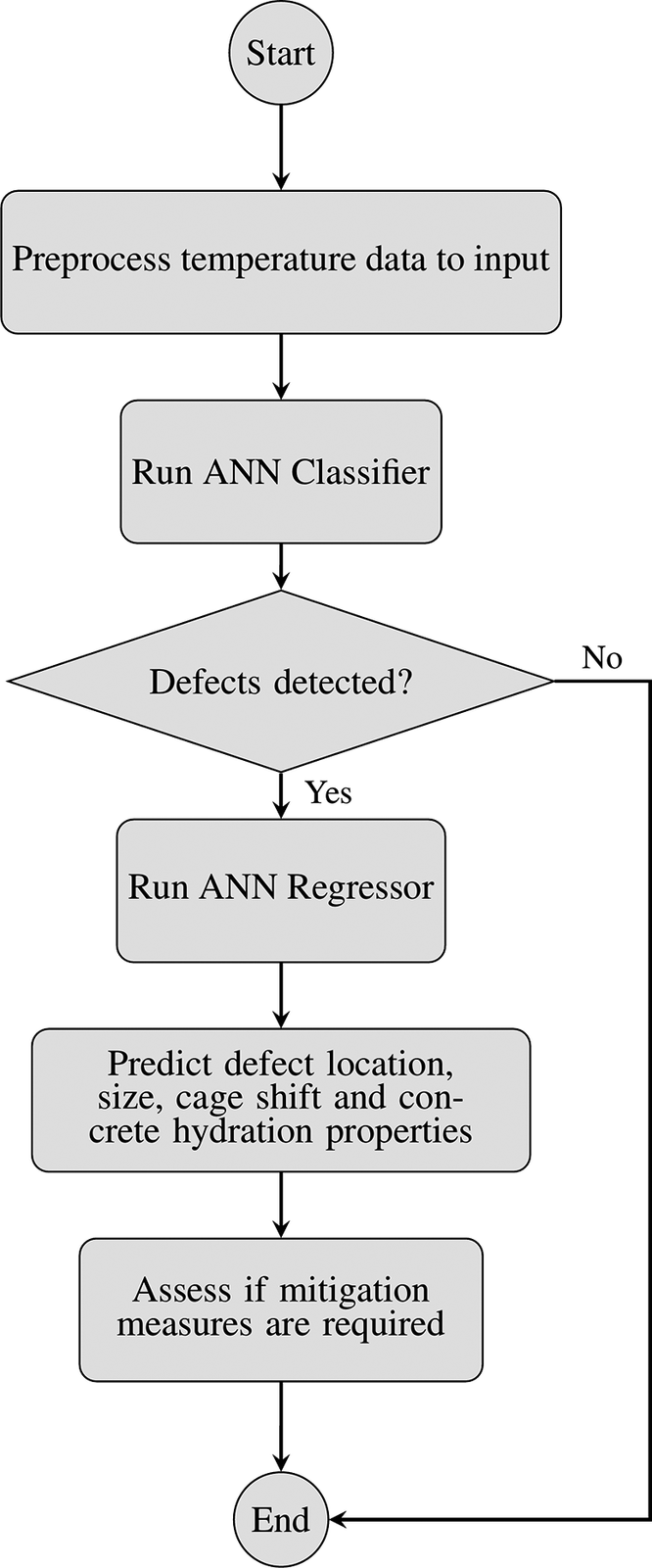
Figure 1. Flowchart of the defect detection model.
2.1. Numerical modeling of HoH
Several theoretical models have been proposed to calculate HoH by considering cement’s chemical reaction kinetics, but they require a large number of parameters (Parrot and Killoh, Reference Parrot and Killoh1984; Kishi and Maekawa, Reference Kishi and Maekawa1996; Swaddiwudhipong et al., Reference Swaddiwudhipong, Chen and Zhang2002). Schindler and Folliard (Reference Schindler and Folliard2005) proposed a model with fewer parameters, where the HoH of a specific mixture can be characterized from the activation energy, the degree of hydration development at the reference temperature, and the total HoH. It makes use of the “equivalent age” concept, described as a way to normalize the concrete curing progress over time, given the varying temperature conditions (Schindler and Folliard, Reference Schindler and Folliard2005). A similar model is proposed by Liu et al. (Reference Liu, Fisher, Taborda and Bourne-Webb2022), which has been calibrated and validated against field measurements of hydration temperature in piles. Numerical modeling of HoH has become a valuable tool in predicting the thermal behavior of concrete during the early stages of curing. Some researchers have computationally modeled the exothermic reaction using empirical equations (Xie and Qian, Reference Xie and Qian2023; Tan and Tang, Reference Tan and Tang2024).
Heat transfer in soils is predominantly governed by conduction, and thus it will be the only mode considered in this study. The transient heat conduction equation is described in Equation (1) as follows:
 $$ \rho {c}_p\frac{\mathit{\partial} T}{\mathit{\partial} t}- k{\boldsymbol{\nabla}}^{\mathbf{2}} T={P}_{hoh} $$
where $ \rho\;\left[ kg\bullet {m}^{-3}\right] $
,
$ \rho\;\left[ kg\bullet {m}^{-3}\right] $
, $ {c}_p\;\left[ J\bullet k{g}^{-1}\bullet {K}^{-1}\right] $
, and
$ {c}_p\;\left[ J\bullet k{g}^{-1}\bullet {K}^{-1}\right] $
, and $ k\;\left[ W\bullet {m}^{-1}\bullet {K}^{-1}\right] $
are the density, volumetric heat capacity, and thermal conductivity of the material, respectively, and
$ k\;\left[ W\bullet {m}^{-1}\bullet {K}^{-1}\right] $
are the density, volumetric heat capacity, and thermal conductivity of the material, respectively, and $ {P}_{hoh}\;\left[ W\bullet {m}^{-3}\right] $
is the HoH power per unit volume, which serves as the only internal heat source. The HoH of concrete curing is calculated herein based on the formulation given in Liu et al. (Reference Liu, Fisher, Taborda and Bourne-Webb2022). This model establishes a relation between the HoH power per unit volume and the accumulated HoH since the start of hydration. The model accounts for key factors, such as the composition of cement, temperature, and reaction kinetics, but with fewer parameters than other models previously mentioned, simplifying its use in practical applications. The key aspects of the model formulation are summarized in the following, with further details available in Liu et al. (Reference Liu, Fisher, Taborda and Bourne-Webb2022).
$ {P}_{hoh}\;\left[ W\bullet {m}^{-3}\right] $
is the HoH power per unit volume, which serves as the only internal heat source. The HoH of concrete curing is calculated herein based on the formulation given in Liu et al. (Reference Liu, Fisher, Taborda and Bourne-Webb2022). This model establishes a relation between the HoH power per unit volume and the accumulated HoH since the start of hydration. The model accounts for key factors, such as the composition of cement, temperature, and reaction kinetics, but with fewer parameters than other models previously mentioned, simplifying its use in practical applications. The key aspects of the model formulation are summarized in the following, with further details available in Liu et al. (Reference Liu, Fisher, Taborda and Bourne-Webb2022).
An S-shaped curve describes the evolution of the reference-accumulated heat per unit mass of cement ( $ {Q}_{ref}\;\left[ J\bullet k{g}_{cement}^{-1}\right] $
) with time (van Breugel, Reference van Breugel1997):
$ {Q}_{ref}\;\left[ J\bullet k{g}_{cement}^{-1}\right] $
) with time (van Breugel, Reference van Breugel1997):
 $$ {Q}_{ref}(t)={Q}_{max}\;{e}^{-{\left(\frac{\tau}{t}\right)}^{\beta}} $$
where $ {Q}_{max}\;\left[ J\bullet k{g}_{cement}^{-1}\right] $
is the maximum accumulated heat per unit mass of cement, and
$ {Q}_{max}\;\left[ J\bullet k{g}_{cement}^{-1}\right] $
is the maximum accumulated heat per unit mass of cement, and $ \beta\;\left[-\right] $
and
$ \beta\;\left[-\right] $
and $ \tau\;\left[ s\right] $
are model parameters to fit observed hydration data.
$ \tau\;\left[ s\right] $
are model parameters to fit observed hydration data.
The heat accumulation law (Equation (2)) is subsequently differentiated with respect to time to establish a power per unit volume, with a further correction being added to introduce the effect of temperature via the activation energy $ {E}_a\;\left[ J\bullet mo{l}^{-1}\right] $
, resulting in:
$ {E}_a\;\left[ J\bullet mo{l}^{-1}\right] $
, resulting in:
 $$ P\left( T, t\right)=\chi {\rho}_{conc}\frac{d{ Q}_{ref}}{ d t}\;{e}^{-\frac{E_a}{R\; T}\;\left[\;\frac{1}{T}-\frac{1}{T_{ref}}\right]}{\left(\frac{Q_{max}-{Q}_{a cc}(t)}{Q_{max}-{Q}_{ref}(t)}\right)}^{n^{\ast }(t)}\hskip0.36em $$
where $ P\left( T, t\right)\;\left[ W\bullet {m}^{-3}\right] $
is the HoH power as a function of time and temperature,
$ P\left( T, t\right)\;\left[ W\bullet {m}^{-3}\right] $
is the HoH power as a function of time and temperature, $ R\;\left[ J\bullet mo{l}^{-1}\bullet {K}^{-1}\right] $
is the universal gas constant, and
$ R\;\left[ J\bullet mo{l}^{-1}\bullet {K}^{-1}\right] $
is the universal gas constant, and $ {n}^{\ast }(t) $
is a factor that encapsulates the effect of reaction kinetics. The accumulated HoH,
$ {n}^{\ast }(t) $
is a factor that encapsulates the effect of reaction kinetics. The accumulated HoH, $ {Q}_{acc}(t) $
, is given by:
$ {Q}_{acc}(t) $
, is given by:
 $$ {Q}_{acc}(t)=\frac{1}{\chi {\rho}_{conc}}{\int}_0^t P\left( T, t\right) d t $$
where $ \chi\;\left[ k{g}_{cement}\bullet k{g}^{-1}\right] $
is the mass of cement per unit mass of concrete and
$ \chi\;\left[ k{g}_{cement}\bullet k{g}^{-1}\right] $
is the mass of cement per unit mass of concrete and $ {\rho}_{conc}\;\left[ kg\bullet {m}^{-3}\right] $
is the concrete density. Solving these equations gives an accurate way to predict the HoH of concrete piles.
$ {\rho}_{conc}\;\left[ kg\bullet {m}^{-3}\right] $
is the concrete density. Solving these equations gives an accurate way to predict the HoH of concrete piles.
Given its relatively simple calibration and reliance on a limited number of parameters, the model is well suited for field applications requiring rapid predictions, such as temperature control during curing and, most importantly, TIP of deep foundations (Liu et al., Reference Liu, Fisher, Taborda and Bourne-Webb2022).
The model was implemented with the heat transfer module in COMSOL Multiphysics, which was used to conduct transient 2D-plan thermal analyses of the HoH process. The 2D approximation assumes that heat fluxes in the out-of-plane direction are negligible due to the large pile depth compared to its other dimensions. This assumption holds because the applied heat and material properties remain constant along the pile depth (for specific soil layers), with heat transfer occurring solely within the plane containing the cross-section. The only exception for this is the end effect, estimated to be of 1-diameter depth (Sun et al., Reference Sun, Elshafie, Barker, Fisher, Schooling and Rui2021). A parametric, time-dependent study is run across different geometric configurations.
The geometry consisted of a concrete pile centered within a circular soil domain of 15 m radius. The boundary condition on the outer edge of the soil domain was set to a constant temperature throughout the simulation. The size of the domain was chosen to be sufficiently large to prevent any boundary effects from affecting the heat distribution on the pile while limiting the computational effort required. The initial temperature across the entire domain was assumed to match that of the poured concrete and was included in the model as an additional variable.
The HoH was modeled only within the concrete pile domain, with heat transfer occurring through conduction in both the concrete and the surrounding soil. In samples where a defect is included, no HoH occurs in this domain. The mesh was generated using second-order triangular elements for solving the heat transfer problem, with a higher resolution applied to the concrete pile and its vicinity. The meshing process was conducted using the COMSOL in-built mesher, and a sample mesh is shown in Figure 2. Given that the model is generated parametrically, several cases considered in this study were inspected to ensure that adequate spatial discretizations were always obtained, particularly when the edge of the defect was located close to that of the pile. Each sample was modeled with ~1,000–1,600 elements, depending on the radius adopted for the pile.
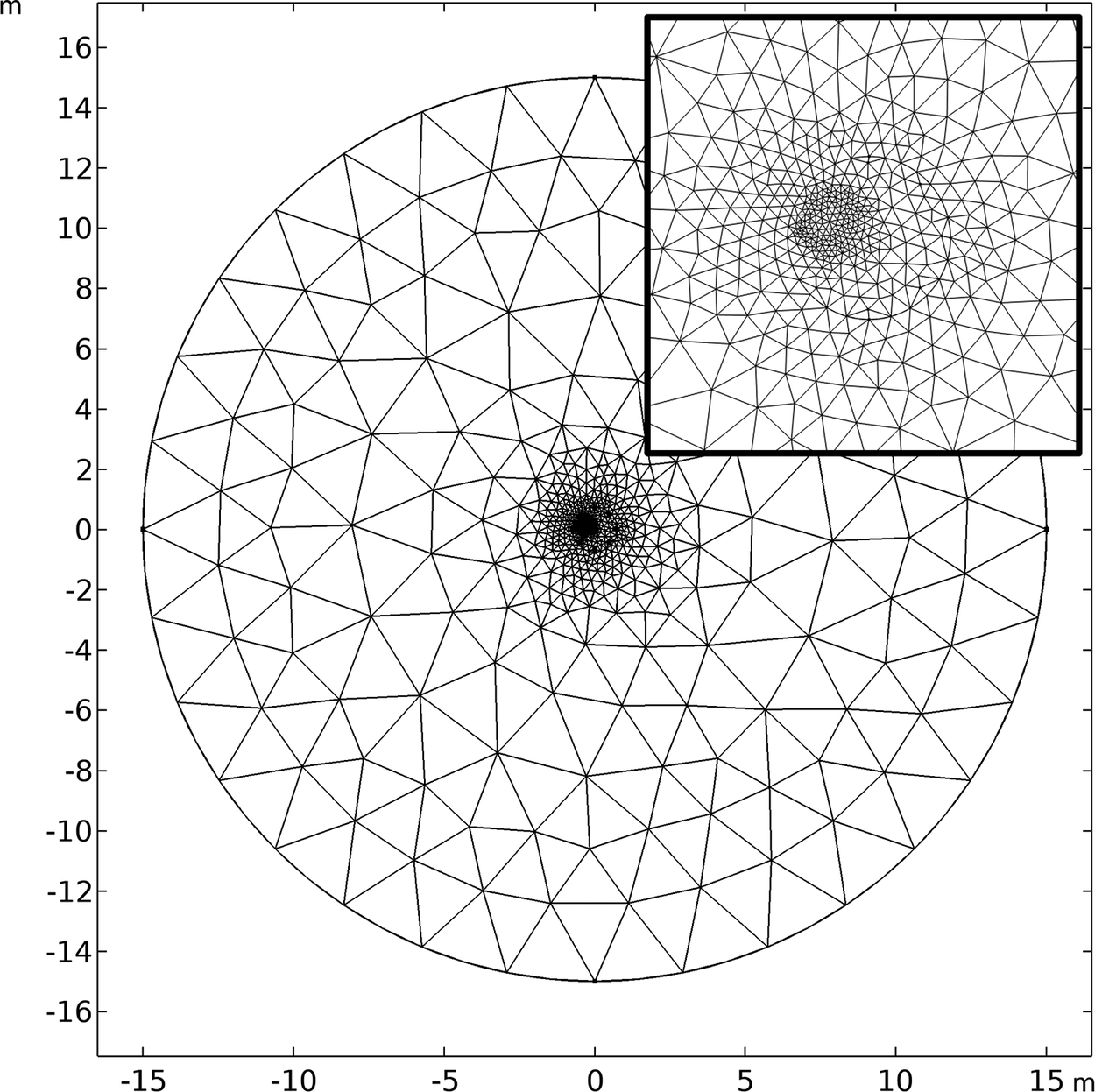
Figure 2. Sample mesh geometry.
2.2. Numerical data
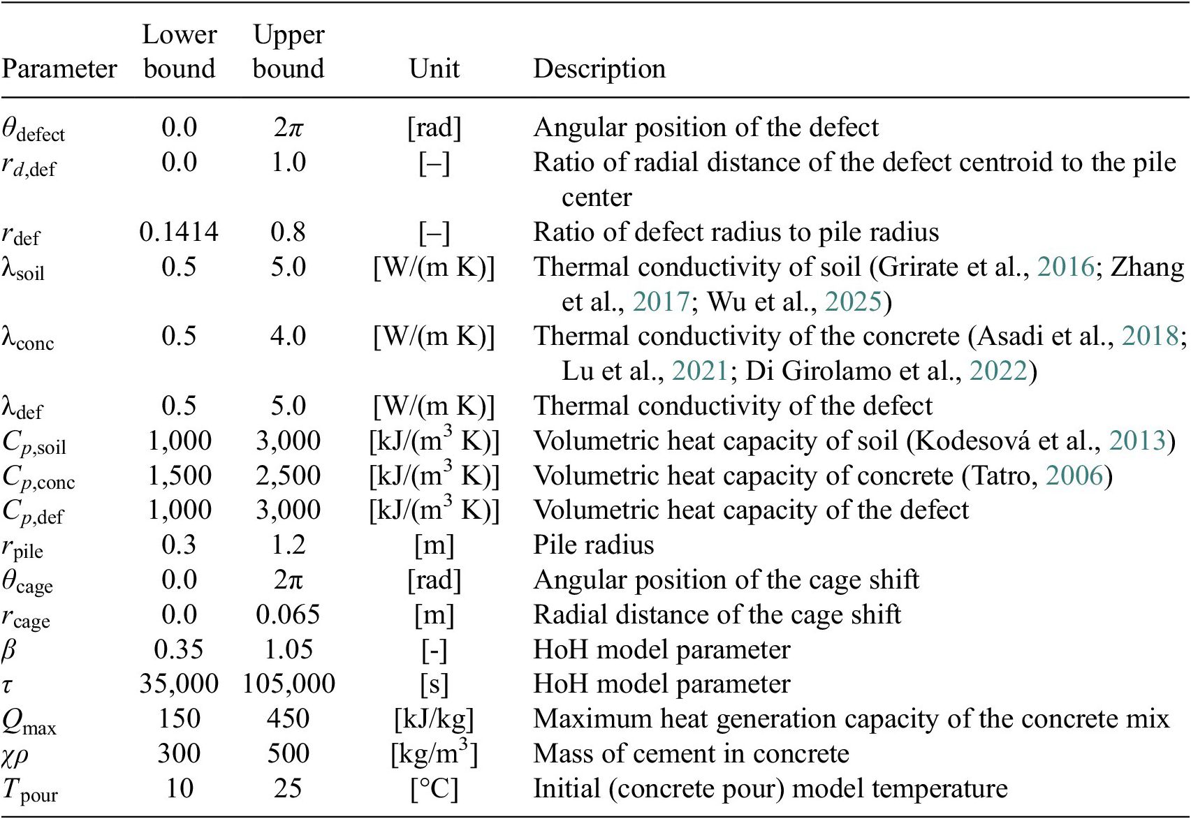
A dataset comprising 100,000 simulations was produced by adopting the numerical model described above. It included variations in a wide range of geometric and material parameters, listed in Table 1. These include the defect geometric properties, thermal conductivities, and volumetric heat capacities of the materials, pile, and cage displacement properties, and hydration model parameters. In this study, material properties are assumed to be homogeneous across the domain. The input values for each of the simulations were established using the near-random Latin hypercube sampling approach. This statistical method, first introduced by McKay et al. (Reference McKay, Beckman and Conover1979), is used to sample points from a multidimensional space, ensuring that each parameter’s range is well represented across the entire dataset. It divides each parameter’s distribution into equal intervals and selects sample points such that all intervals are covered without repetition, improving sampling efficiency in large models. This ensured that all geometric and material parameter combinations were representative of the real-world variability of data in a computationally efficient way, thereby enabling the model to predict defects among a wide range of soil, concrete, and defect types. The lower and upper bounds for each of the parameters being varied are provided in Table 1. The parameter range defined by these bounds was deliberately made very large, hence ensuring that they covered any potential parameter combination to be encountered in practice. Even though some combinations are unlikely to occur in real-life conditions, this broader range is beneficial for the generalization of the model, thus preventing overfitting to a narrow subset of conditions.
Table 1. Numerical model parameters
Soil or bentonite defects were modeled as circles in the cross-sectional plane. Complex defect shapes were not evaluated throughout this study, as the impact of a defect on the HoH generation is more dependent on its area (or volume when considering three-dimensional [3D] problems) rather than its shape. Only defects with an equivalent area >2% of the pile cross-sectional area were considered, as the temperature variations generated by smaller defects would be too small to allow identification, particularly when these are located away from the probes, that is, toward the center of the pile. Furthermore, it could be argued that these are not defects at all. In turn, the largest modeled radius of the defect is 80% of that of the pile (i.e., equivalent to 64% of the total pile area). Due to the randomized nature of the defect parameter generation, the defect-to-pile radius ratios follow a uniform distribution. When these ratios are converted to defect radii and the associated defect areas are calculated, 53% of defects have an equivalent area of <20% of the pile’s cross-sectional area, thus aligning with the most commonly observed defect size in practice (Sarhan et al., Reference Sarhan, Tabsh, O’Neill, Ata, Ealy, O’Neill and Townsend2002; Sun et al., Reference Sun, Elshafie, Xu and Schooling2024). The material properties of the defect are generated independently from the surrounding soil or concrete, accounting for other alternatives, such as loose soil or bentonite.
In order for the dataset to be most relevant to real-world scenarios, where the presence of a defect within the pile would not be known a priori, samples with and without defects were included. This approach enables the ANN models to generalize beyond defect-only cases, producing predictions that are more robust.
Temperature values were measured across eight probe locations spaced radially at equal angles, as shown in Figure 3. The temperature probes are located near the edge of the concrete pile, leaving a 75 mm cover. As the outer part of the shaft is the most relevant for its bending capacity, identifying defects in these regions is particularly important (Mullins, Reference Mullins2010). Temperature values from each of these probe locations were stored every 0.05 days for the first 5 days after pouring, leading to 101 temperature values per probe, per sample. A node was placed at each of the probe locations such that the temperature values were established directly from the FE calculation, rather than relying on interpolation.
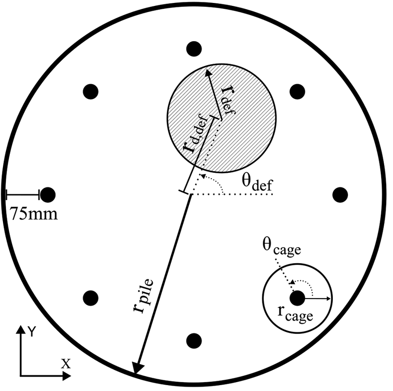
Figure 3. Pile and defect geometry.
A total of 586 parameter combinations, including a defect, could not be computed because of meshing complications; they all corresponded to cases where the edge of the defect was very close to one of the probes. The affected samples represent ~0.6% of the total. Latin hypercube sampling ensures that samples are distributed across the entire range of the input variables, making it robust to small changes (Forrester et al., Reference Forrester, Sóbester and Keane2008). This suggests that even if a few samples are removed, the remaining dataset can still be representative of the design space due to the stratified nature of the sampling technique, and therefore, the parameters can still be assumed to be randomly distributed.
When pile rebar cages are inserted into bored piles, they can displace from the design position. To account for this effect, two parameters, $ {\theta}_{cage} $
and
$ {\theta}_{cage} $
and $ {r}_{cage} $
are generated to simulate the potential cage shift as a function of the angular direction and radial distance from the origin. These define the angle of cage shift and its magnitude, ranging between 0–2π and 0–6.5 cm, respectively.
$ {r}_{cage} $
are generated to simulate the potential cage shift as a function of the angular direction and radial distance from the origin. These define the angle of cage shift and its magnitude, ranging between 0–2π and 0–6.5 cm, respectively.
The defect area and the centroid’s Cartesian coordinates were calculated analytically. Defects could overlap the soil domain, potentially leading to noncircular shapes. In cases when these defects partly extend beyond the edge of the concrete pile, they were trimmed such that only the portion originally within the concrete section was considered as defect, with the material properties being assigned accordingly, whereas the remaining portion of the circle (i.e., outside the concrete section) was assumed to be soil. The area and centroid coordinates were then calculated using Monte Carlo integration, a statistical method commonly used to estimate the area of complex shapes, although analytical solutions exist for this specific geometric problem. This involves the random sampling of points ( $ {N}_{tot} $
) within the region bounded by the concrete pile and defect, and counting how many falls within the intersecting section. The proportion of points (
$ {N}_{tot} $
) within the region bounded by the concrete pile and defect, and counting how many falls within the intersecting section. The proportion of points ( $ {N}_{in} $
) that fall within the intersection of the two circles (pile and defect) was used to estimate the area of the defect (Equation (5)), while the average coordinate of the points inside the intersection provided an estimate of the section centroid, as shown in Equations (6) and (7). To produce accurate area and centroid estimations, four million points were randomly generated for each sample.
$ {N}_{in} $
) that fall within the intersection of the two circles (pile and defect) was used to estimate the area of the defect (Equation (5)), while the average coordinate of the points inside the intersection provided an estimate of the section centroid, as shown in Equations (6) and (7). To produce accurate area and centroid estimations, four million points were randomly generated for each sample.
 $$ A\approx \frac{N_{in}}{N_{tot}}\bullet {A}_{bound} $$
 $$ {x}_c=\frac{1}{A}{\int}_A x\; dA\approx \frac{1}{N}{\sum}_{i=1}^N{x}_i $$
 $$ {y}_c=\frac{1}{A}{\int}_A y\; dA\approx \frac{1}{N}{\sum}_{i=1}^N{y}_i $$
2.3. ML model
In order to develop the proposed methodology for defect detection in bored piles using TIP, two ANN models were created: the first to establish whether a defect is present, and the second to estimate the defect size and location, cage shift, and concrete properties of the sample pile when a defect is identified. Figure 4 summarizes the process to generate data and train the ANN. The ANN models were built using the deep learning package Keras (Chollet, Reference Chollet2021) and the procedures employed to do so are detailed in the following.
Figure 4. Flowchart showing the ANN creation process.
2.3.1. Data processing and ML inputs
The FE output for all samples and probes was preprocessed before being passed to the ML training process. To decide on the model inputs, a statistical analysis of temperature values was conducted for each probe, including the maximum temperature recorded at any time, the average temperature over the 5-day simulation period, the maximum temperature differences between all probes, and the time instants at which these maximum temperatures occurred. The concrete ratio of the mix, initial temperature, and pile radius were also used for model training. These were included as inputs for both the classification and regression modes. In addition to those inputs, the regression ANN model also incorporated temperature data recorded at intervals of every 0.25 days between t = 0.25 and t = 2 days, as well as at t = 3, 4, and 5 days for each probe. It is worth noting that by using exclusively temperature values as inputs to the ANN models, the proposed approach does not require any field or laboratory testing to assess hydration parameters, which are, in fact, returned by the regression ANN. The dataset used throughout this publication is available on Sánchez Fernández (Reference Sánchez Fernández2025).
To maximize the performance of the models, it is important to consider the different input parameters that have the greatest impact on the resulting output. Spearman’s correlation coefficient ( $ {r}_s $
, see Equation (8)) was used to study these relationships. This coefficient measures the relationship between two continuous variables, ranging from −1 to +1. Unlike Pearson’s correlation coefficient, which assumes a linear relationship and normally distributed data, Spearman’s correlation coefficient measures the monotonic relationship between two variables, regardless of whether they are linear or not, by comparing their rank orders instead of their actual values. Spearman’s correlation is more robust to outliers than Pearson’s, as it evaluates the relative ranking of the data points rather than their magnitude (Moscarelli, Reference Moscarelli2023).
$ {r}_s $
, see Equation (8)) was used to study these relationships. This coefficient measures the relationship between two continuous variables, ranging from −1 to +1. Unlike Pearson’s correlation coefficient, which assumes a linear relationship and normally distributed data, Spearman’s correlation coefficient measures the monotonic relationship between two variables, regardless of whether they are linear or not, by comparing their rank orders instead of their actual values. Spearman’s correlation is more robust to outliers than Pearson’s, as it evaluates the relative ranking of the data points rather than their magnitude (Moscarelli, Reference Moscarelli2023).
 $$ {r}_s=1-\frac{6\sum {d}_i^2}{n\left({n}^2-1\right)} $$
In Equation (8), $ {d}_i $
is the difference in the ranks of corresponding data points, and
$ {d}_i $
is the difference in the ranks of corresponding data points, and $ n $
is the number of data points. Figure 5 shows the Spearman’s correlation coefficients for the regression model inputs and outputs, while Figure 6 presents the Spearman’s correlation coefficient for the input variables of the classifier algorithm. Each individual cell in the heatmap corresponds to a probe value within the overall cluster. The results indicate that most variables exhibit weak correlations, except for the average and maximum temperatures, which are naturally highly correlated as they arise from the same time series. Despite their correlation, these inputs are essential for capturing the characteristics of the temperature field within the hydrating pile problem, which is fundamental to the model’s performance at predicting the presence, size, and location of defects.
$ n $
is the number of data points. Figure 5 shows the Spearman’s correlation coefficients for the regression model inputs and outputs, while Figure 6 presents the Spearman’s correlation coefficient for the input variables of the classifier algorithm. Each individual cell in the heatmap corresponds to a probe value within the overall cluster. The results indicate that most variables exhibit weak correlations, except for the average and maximum temperatures, which are naturally highly correlated as they arise from the same time series. Despite their correlation, these inputs are essential for capturing the characteristics of the temperature field within the hydrating pile problem, which is fundamental to the model’s performance at predicting the presence, size, and location of defects.
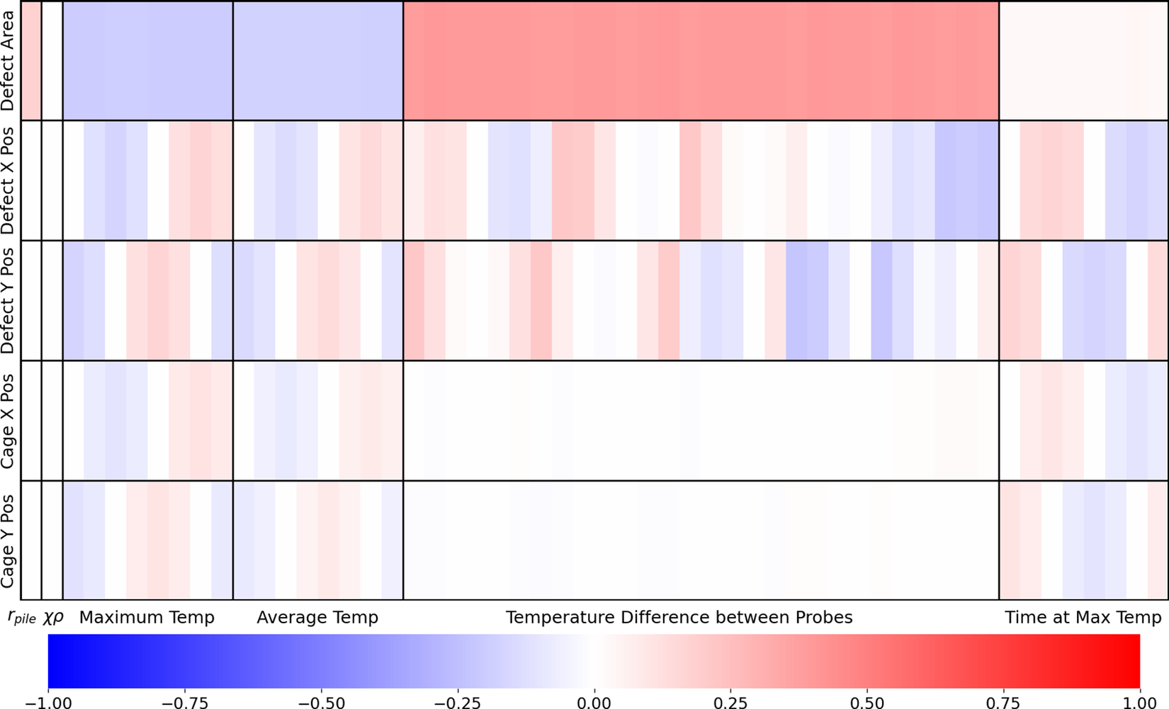
Figure 5. Spearman’s correlation coefficient between the model inputs and outputs.
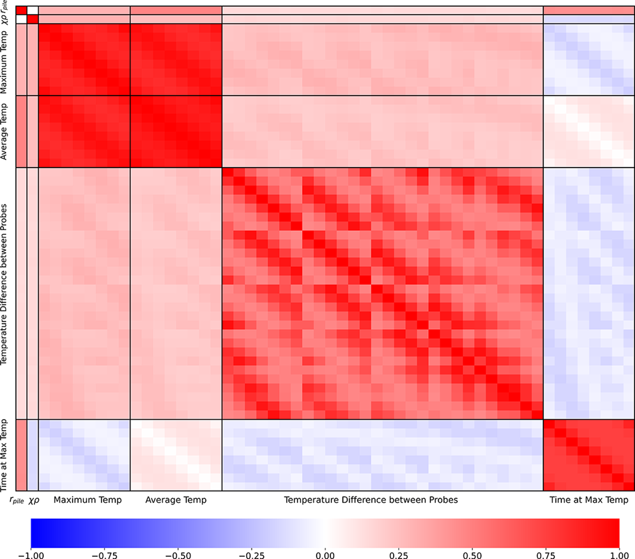
Figure 6. Spearman’s correlation coefficient for the model inputs.
In addition to the possibility of reinforcement cage misalignment, which affects the position at which temperatures are measured, the accuracy of temperature readings for TIP is a critical consideration. Measurement inaccuracies can significantly affect the thermal profiles and their subsequent assessment and interpretation. Introducing noise serves as a powerful generalization mechanism that improves the reliability of ML outputs by simulating the variability typically observed in real-world data (Vogt et al., Reference Vogt, Mottaghy, Wolf, Rath, Pechnig and Clauser2010). By adding controlled perturbations to the raw deterministic data, the model learns patterns more robustly, leading to reduced overfitting. In TIP measurements, most of the noise comes from the sensor accuracy during testing.
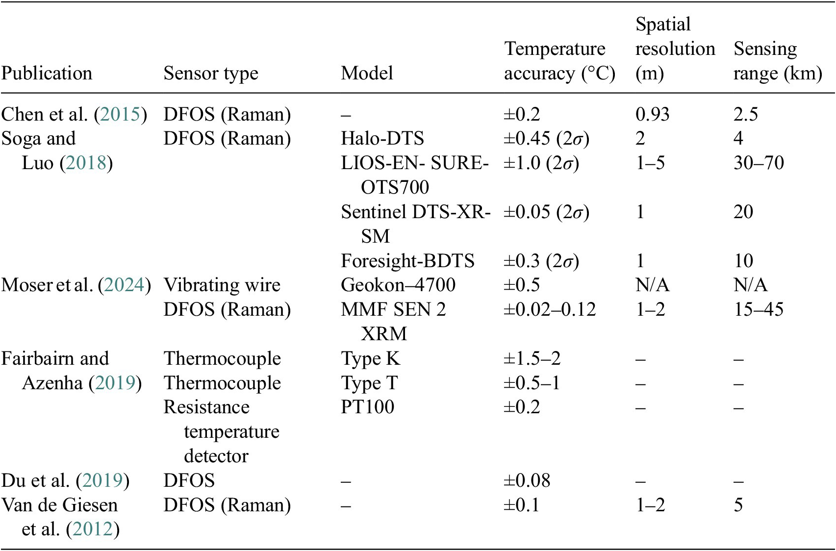
Raman-based distributed fiber optic sensors (DFOS) are the preferred choice when using nondestructive integrity evaluation techniques such as DTS (Hartog, Reference Hartog2017). Some distributed temperature-sensing models, such as the Sentinel DTS, can achieve temperature measurement accuracies as fine as 0.01°C, with resolutions of 1 m for up to 45 km (Sensornet, 2021). Other sensors, summarized in Table 2, also provide very high accuracies and resolutions. In addition to sensor accuracy, in practice, spatial resolution (SR) plays a large role in DFOS temperature readings (Bao and Chen, Reference Bao and Chen2012). Since Raman-based DFOS returns a weighted average temperature across its SR, discrepancies between actual and measured temperatures can arise (Pradhan and Sahu, Reference Pradhan and Sahu2015). However, as the model in this study relies on 2D numerical data, SR effects cannot be explicitly incorporated. Therefore, to account for these effects, a normally distributed noise with a standard deviation of 0.1°C will be added to all temperature readings, resulting in 99.7% of the noise values being within ±0.3°C. This level of accuracy, in line with that of the sensors listed in Table 2, aids in ensuring the generalization of the ML model while maintaining realistic conditions for TIP. Introducing greater variation would potentially result in predictions that would be unreasonably inaccurate when compared to those in the field, as high-accuracy equipment is an inherent requirement for the method, both with respect to SR and sensor accuracy.
Table 2. Summary of different temperature sensor accuracies as reported in the literature
2.3.2. Classification algorithm
An ANN was developed to perform the binary classification of piles into defective and nondefective, using the “KerasClassifier” algorithm. The dataset was split into training, validation, and testing sets, using an 80-10-10 split to ensure sufficient data is provided for both model training and validation. In terms of the number of samples, this corresponds to 79531-9941-9942. Before training, all input features were standardised using z-score normalization. The architecture of the ANN was established following a grid search approach (Raschka, Reference Raschka2017). The best architecture was identified based on its performance from a 10-fold cross-validation. It consisted of three densely connected hidden layers with neuron counts of 3,000, 1,500, and 300, respectively. Rectified linear unit (ReLU) activation functions were used in all hidden layers, allowing the model to learn nonlinear patterns in the data. A sigmoid activation function was applied to the output layer to perform binary classification (defect or no defect). The loss function was set to binary cross-entropy. The model was trained using the Adam optimizer with an initial learning rate of 0.001. A learning rate reduction strategy was also implemented, where the learning rate was reduced by a factor of 0.1 if no improvement was observed in validation loss for five consecutive epochs. The model was trained using a batch size of 800 samples and a maximum of 150 epochs. To mitigate overfitting, a dropout rate of 0.4 was applied to each hidden layer. In addition, early stopping was implemented, stopping the training process if no improvement in validation loss was detected after 10 epochs. This prevented overfitting by ensuring the model did not continue training once it had sufficiently learned from the data.
The resulting defect-labeled samples, both true and false positives, are then passed on to the regressor to evaluate each sample further.
2.3.3. Regression algorithm
The regression algorithm presents a similar structure in complexity compared to the classifier. The algorithm chosen for this task was “KerasRegressor.” This regressor was trained to predict the size and location ( $ x $
and
$ x $
and $ y $
coordinates) of defects within the pile cross-section, potential cage shifts, and back-analyze three concrete HoH parameters:
$ y $
coordinates) of defects within the pile cross-section, potential cage shifts, and back-analyze three concrete HoH parameters: $ \beta $
,
$ \beta $
, $ \tau $
, and
$ \tau $
, and $ {Q}_{max} $
.
$ {Q}_{max} $
.
The configuration of the model included three densely connected hidden layers with 1,500, 750, and 250 neurons, respectively, each using ReLU activations. Batch normalization was applied after each hidden layer to improve training stability, along with a dropout rate of 0.4. The regressor was trained using the Adam optimizer with a learning rate of 0.001 and a batch size of 400 samples over 150 epochs. Reduced learning rate and early stopping were also included. The model’s loss function was the mean squared error (MSE) function, as shown in Equation (9). The model was trained on the same dataset as the classifier and subsequently validated and tested on the true and false positive samples labeled by the classifier. This produced an environment that not only determines the presence of inclusions, but also characterizes their size and location.
 $$ MSE=\frac{1}{n}{\sum}_{\left\{ i=1\right\}}^n{\left({x}_i-{\hat{x}}_i\right)}^2 $$
3. Results and discussion
3.1. Classification ANN
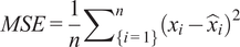
A total of 9,942 samples were used to evaluate the performance of the classification ANN model. The confusion matrix for the test set, shown in Figure 7, demonstrates the excellent classification ability of the model: about 94% of the samples were classified correctly. The model only misidentified a limited number of pile samples with defects, mislabeling 571 of these as false negatives (i.e., the classifier indicates the absence of a defect when there was indeed one). The number of false positives is lower in comparison, mislabeling 77 samples (i.e., the classifier returns the existence of a defect when one was not present). The receiver operating characteristic (ROC) curve, shown in Figure 8, further illustrates the model’s effectiveness by depicting its true positive rate against the false positive rate at various threshold levels. The area under the curve (AUC) is 0.97, indicating a high level of classification accuracy (a value of 0.5 would indicate that the classification was as good as a random guess and 1.0 would suggest perfect classification).
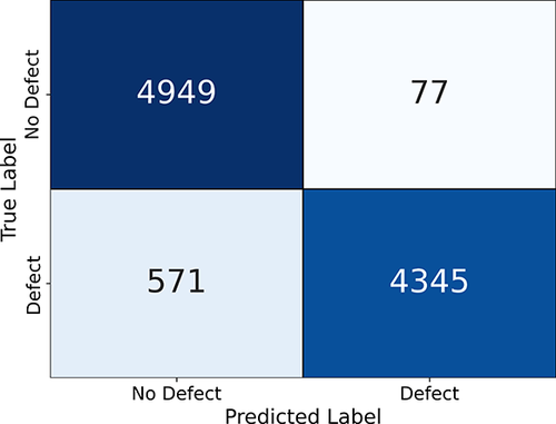
Figure 7. Confusion matrix for the test set.
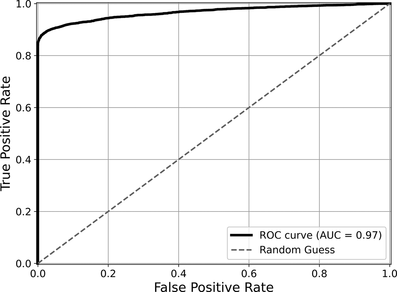
Figure 8. ROC curve for the test set.
Figure 9 presents the accuracy curve for the training and validation datasets. These curves serve as useful indicators of potential overfitting. Consistent with the above, the model shows very good predictive performance. The obtained training and validation accuracies are 0.938 and 0.935, respectively, suggesting that the model is effectively capturing patterns in the data without overfitting. This allows the model to generalize well to new, unseen data.
Figure 9. Train and validation accuracy for each epoch.
An attempt was made to lower the classifier’s decision threshold to reduce the number of false negatives. However, the model exhibited a high degree of confidence in its false negative predictions. Adjusting the decision threshold, therefore, provides no meaningful improvement in model performance, as the false positive rate increases by similar amounts as the false negative decreases.
Figure 10 shows the model’s accuracy at predicting defect samples based on their radial distance from the center of the pile; for reference, samples have been grouped in bins of equal width, and the 90% accuracy mark is indicated by the solid red line. As expected, given the location of the probes, the model struggles to identify some of the defects located within the central 20% of the pile’s radius. In contrast, for defects situated in the outer 80% of the pile’s radius (or 96% of the equivalent pile area), the model’s accuracy is nearly perfect. This trend aligns with the findings of Boeckmann and Loehr (Reference Boeckmann and Loehr2019), who observed that TIP techniques tend to underperform when attempting to detect inclusions within the interior of the reinforcement cage, that is, at locations distant from measurement optic cables.
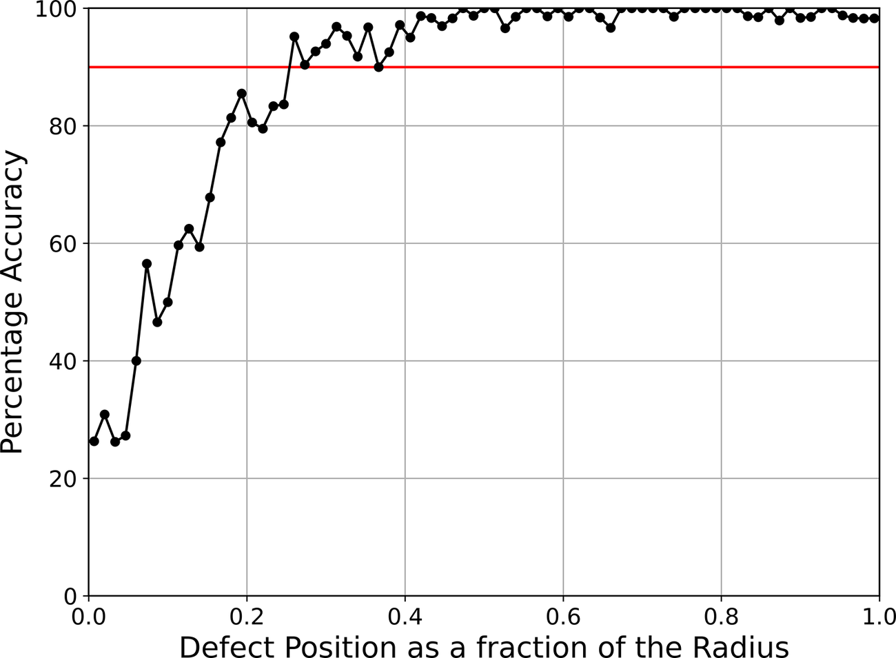
Figure 10. Accuracy versus defect radial position for defect-labeled samples.
When evaluating the model’s performance across defects categorized by relative and nominal area, as shown in Figures 11 and 12, defect size is shown to play an important role. In effect, the model demonstrates higher accuracy for larger defects, consistent with the expectation that larger anomalies generate more distinguishable disturbances in the temperature field, making it easier for the model to classify correctly.
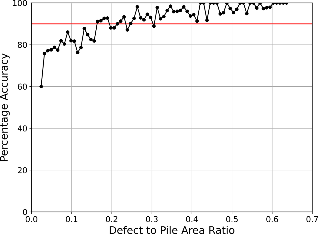
Figure 11. Accuracy versus defect area–pile ratio for defect-labeled samples.
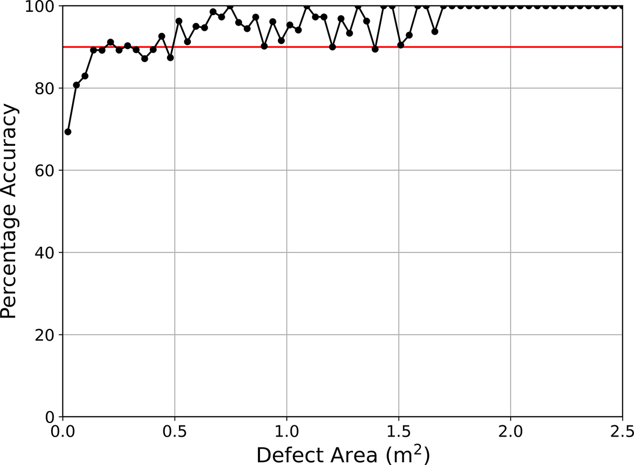
Figure 12. Accuracy versus defect area for defect-labeled samples.
Smaller defects are likely to produce only subtler disturbances in the temperature distribution, which, added to the additional noise included artificially, lead to a higher rate of misclassification. For a target accuracy of 0.9, the existence of defects with areas >0.17 m2 (0.23 m radius) will be correctly predicted. Even the smallest defects, with an area of ~0.05 m2 (0.12 m radius), are detected with over 70% accuracy.
Ashlock and Fotouhi (Reference Ashlock and Fotouhi2014) conclude that a lower bound of at least 8% in relative area is required for TIP to predict inclusions accurately, as these produce barely detectable temperature differences. In this respect, TIP performance is proven to be similar to that of other common pile integrity testing methods such as CSL. Li et al. (Reference Li, Zhang and Tang2005) report that the minimum detectable defect size ranges between 2 and 7% of the pile cross-sectional area, with defects with radii smaller than 0.1 m being undetectable. According to that study, achieving a target accuracy of 0.9 requires defect sizes ranging from 7.5 to 15% of the pile area, which is similar to the results of the ML model presented herein. Amir and Amir (Reference Amir, Amir, Iskander, Laefer and Hussein2009) performed a CSL test on a pile with three artificial defects and concluded that flaws are only detectable between access tubes if they are >10% of the pile cross-sectional area.
Clearly, despite the results suggesting that the classification model has a lower prediction accuracy for defects located toward the pile center and of reduced size, a very high accuracy can be achieved for all types of soil, concrete, and defect characteristics.
The previous results show that most cases where the model misclassifies a defective pile share one condition: the defects are located at, or close to, the pile center. By excluding all samples located within the central section defined by 20% of the pile radius, near-perfect accuracy is achieved, as depicted in Figure 13. This further confirms that the primary limitation of TIP in defect classification is the proximity to the nearest probe rather than defect size. TIP’s overall accuracy would significantly increase should a central optic cable be installed in the pile being monitored. To further corroborate this statement, an additional study was carried out where a ninth fiber optic cable is included at the pile center, whose results are shown in Section 3.3.
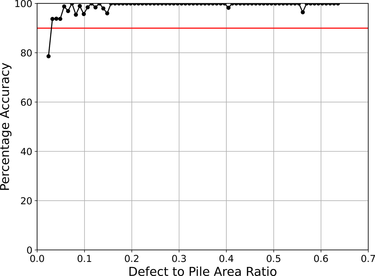
Figure 13. Accuracy versus defect area–pile ratio for samples in the outer 80% of the radial distance.
3.2. Regression ANN
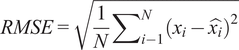
The regression model was tested on 4,422 positive-labeled samples, 77 of which were false positives returned by the classifier. The performance metrics used to evaluate the results are the root MSE (RMSE), the mean absolute error (MAE), and the coefficient of determination ( $ {R}^2 $
), defined in Equations (10)–(12), respectively. In these expressions,
$ {R}^2 $
), defined in Equations (10)–(12), respectively. In these expressions, $ {x}_i $
represents the true value,
$ {x}_i $
represents the true value, $ \hat{x_i} $
is the predicted value,
$ \hat{x_i} $
is the predicted value, $ S{S}_{residual} $
is the sum of squared residuals, and
$ S{S}_{residual} $
is the sum of squared residuals, and $ S{S}_{total} $
is the total sum of squares. Clearly, given their definitions, better predictions are characterized by values of RMSE and MAE closer to 0 and
$ S{S}_{total} $
is the total sum of squares. Clearly, given their definitions, better predictions are characterized by values of RMSE and MAE closer to 0 and $ {R}^2 $
values closer to 1. The errors and performance results for all predicted output variables are provided in Table 3.
$ {R}^2 $
values closer to 1. The errors and performance results for all predicted output variables are provided in Table 3.
 $$ RMSE=\sqrt{\frac{1}{N}{\sum}_{i-1}^N{\left({x}_i-\hat{x_i}\right)}^2} $$
 $$ MAE=\frac{1}{N}{\sum}_{i-1}^N\left|{x}_i-\hat{x_i}\right| $$
 $$ {R}^2=1-\frac{S{S}_{residual}}{S{S}_{total}} $$
Table 3. Regressor performance metrics for the test dataset
Figure 14 shows the real versus predicted values for the output variables. Predictions are particularly accurate for the defect position and area, arguably the most important parameters to identify. The cage misalignment was identified within 7-mm precision, and the defect position within 4 mm, as given by the MAE. The back-calculation of the concrete HoH parameters presents lower accuracies, particularly the parameter controlling the heat evolution over time, $ \tau $
, and the maximum heat generated per unit of mass,
$ \tau $
, and the maximum heat generated per unit of mass, $ {Q}_{max} $
. However, while this information can be useful to predict the hydration response of other structures using the same concrete mix, these values are naturally less important as an outcome of a TIP analysis, where the focus is necessarily on the prediction of the characteristics of any existing defect.
$ {Q}_{max} $
. However, while this information can be useful to predict the hydration response of other structures using the same concrete mix, these values are naturally less important as an outcome of a TIP analysis, where the focus is necessarily on the prediction of the characteristics of any existing defect.
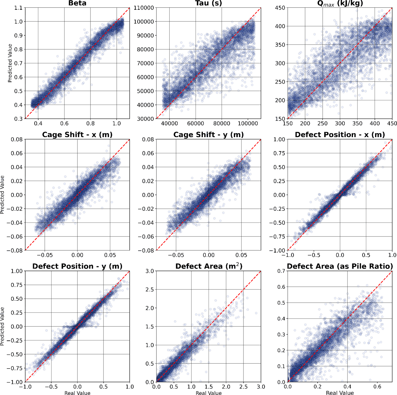
Figure 14. Correlation between real and predicted variables for 4,422 samples.
Overall, the model captures general trends with very high accuracy, despite the artificial noise added to the data and the broad range considered for all parameters. Figure 15 shows the graphical comparison of the real and predicted defects, along with the rebar cage shift, for five samples representing the 10th, 25th, 50th, 75th, and 90th percentiles in percentage error performance. Samples in the lower percentiles predict defects smaller than the real value. The opposite is true for higher percentiles, with the 50th percentile representing an accurately predicted sample. To assess the impact of these prediction inaccuracies on the thermal profile of the samples, the temperature evolution was recalculated in the FE model using the new predicted values for predicted defect size, location, and reinforcement cage shift. These are shown in Table 4. Despite slight inaccuracies in defect characterization, temperature discrepancies are negligible, staying below 1°C for all samples and temperature statistical variables.
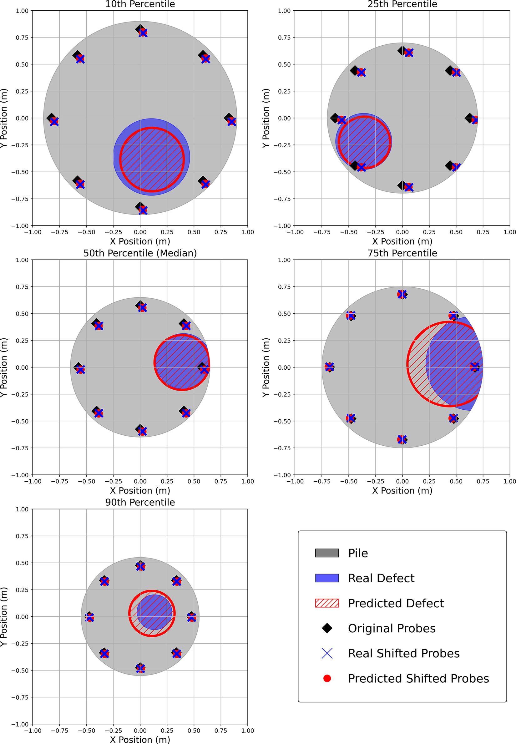
Figure 15. Graphical representation of predicted and real defects and cage displacements for five representative samples.
Table 4. Comparison of hydration temperature values caused by real and predicted defects and cage displacements for five samples selected based on the associated error
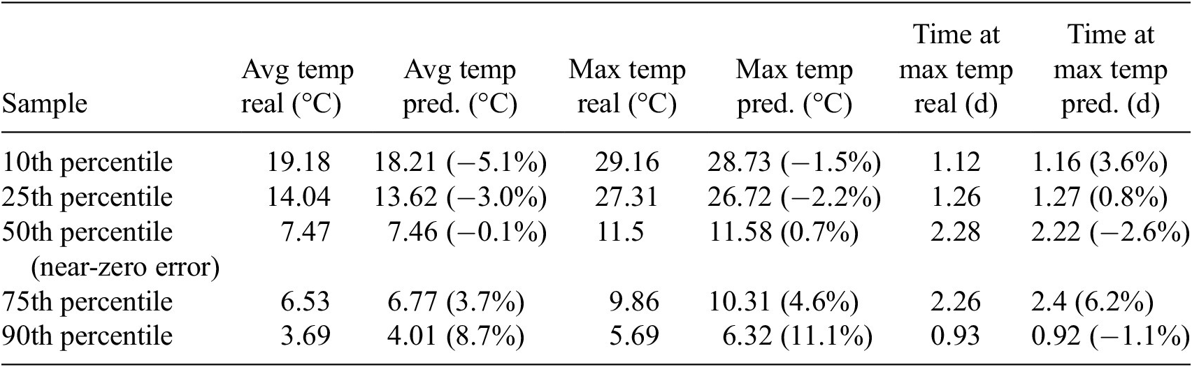
Figure 16 illustrates the real and predicted defect to pile area ratios, with each sample represented by a dot color-coded according to its distance from the pile center. Consistent with the findings in Section 3.1, the size of a significant number of central defects is substantially underestimated in size. This is because the temperature at the sensors does not clearly reflect the presence of the defects, and therefore, the ANN could not learn the patterns as well as for defects closer to the sensors. In some cases, these central defects are difficult to predict by the regressor, as the model likely interprets the overall lack of heat as resulting from factors like a reduced $ {Q}_{max} $
or elevated thermal conductivity, rather than from a significant absence of concrete mass. Consequently, the model predicts near-zero defect sizes for these samples, even though some of them are large. Conversely, a few smaller defects closer to the pile edge are slightly overestimated in size.
$ {Q}_{max} $
or elevated thermal conductivity, rather than from a significant absence of concrete mass. Consequently, the model predicts near-zero defect sizes for these samples, even though some of them are large. Conversely, a few smaller defects closer to the pile edge are slightly overestimated in size.
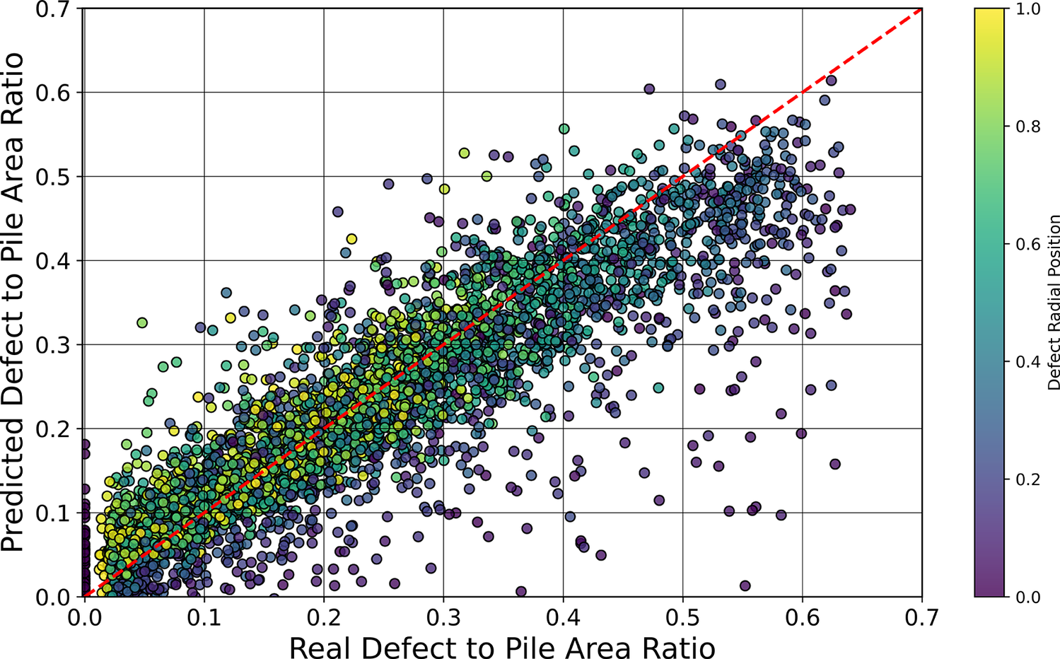
Figure 16. Correlation between real and predicted defect-to-pile area ratio, with samples colored based on radial distance to pile center.
Figure 17 shows the model loss function (MSE), over the training process of 150 epochs. The similarity between the error obtained for the training and validation sets is indicative of the good generalization ability of the model to unseen data.
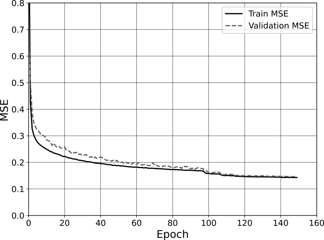
Figure 17. Evolution of training and validation loss with epochs.
3.3. Additional central probe
To address the challenge of mislabeled samples concentrated near the center of the concrete pile, training both the classifier and regressor models by incorporating data from a central fiber optic probe was explored. Integrating a central probe within standard rebar cages can be challenging due to installation complexity, making its feasibility dependent on project-specific considerations and contractor discretion. This section highlights the improvements in terms of predictive performance that can be expected by adding a central probe in TIP experiments, thus informing potential future adaptations to this methodology.
The classifier and regressor models were configured as described in Sections 2.3.2 and 2.3.3. With the inclusion of central fiber optic data, the test accuracy of the classification model increased, yielding an $ {R}^2 $
value of 0.974 (up from 0.935). Figures 18 and 19 show the confusion matrix and the training and validation loss curves during the training process, respectively. The false positive rate decreased by 38% compared to the original model, where only radial probes were used, while the false negative rate saw a reduction of 63%. The training and validation
$ {R}^2 $
value of 0.974 (up from 0.935). Figures 18 and 19 show the confusion matrix and the training and validation loss curves during the training process, respectively. The false positive rate decreased by 38% compared to the original model, where only radial probes were used, while the false negative rate saw a reduction of 63%. The training and validation $ R{}^2 $
scores reached 0.980 and 0.978, respectively, indicating that overfitting is not expected to have taken place. Furthermore, the area under the ROC curve (AUC) increased from 0.97 to 0.99 by adding the central probe. This shows how adding the additional central probe can improve the model’s ability to detect accurately the presence or absence of defects.
$ R{}^2 $
scores reached 0.980 and 0.978, respectively, indicating that overfitting is not expected to have taken place. Furthermore, the area under the ROC curve (AUC) increased from 0.97 to 0.99 by adding the central probe. This shows how adding the additional central probe can improve the model’s ability to detect accurately the presence or absence of defects.
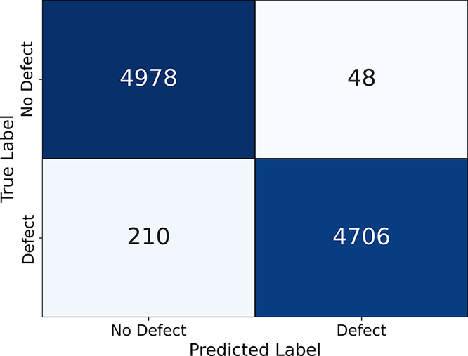
Figure 18. Confusion matrix for the nine-probe test.
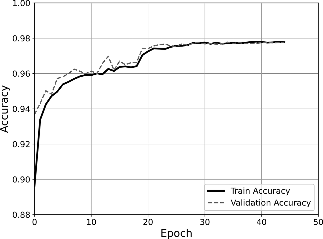
Figure 19. Train and validation accuracy for each epoch, for the nine-probe test.
The results in terms of accuracy versus defect area are presented in Figure 20. The target accuracy is now reached for samples with defect areas larger than 0.07 $ {m}^2 $
, which is considerably smaller than the 0.17
$ {m}^2 $
, which is considerably smaller than the 0.17 $ {m}^2 $
required by the original model. Indeed, defects with an area exceeding 0.14
$ {m}^2 $
required by the original model. Indeed, defects with an area exceeding 0.14 $ m{}^2 $
were detected with near-perfect accuracy. When considering defect to pile area ratios, the minimum defect sizes are found to be 3 and 6% for target accuracies of 0.8 and 0.9, respectively. The results agree with the conclusions presented by Sun et al. (Reference Sun, Elshafie, Xu and Schooling2024), who identified the minimum detectable defect area to be 4–5% of the pile cross-sectional area when using eight radial and one central fiber optic cables.
$ m{}^2 $
were detected with near-perfect accuracy. When considering defect to pile area ratios, the minimum defect sizes are found to be 3 and 6% for target accuracies of 0.8 and 0.9, respectively. The results agree with the conclusions presented by Sun et al. (Reference Sun, Elshafie, Xu and Schooling2024), who identified the minimum detectable defect area to be 4–5% of the pile cross-sectional area when using eight radial and one central fiber optic cables.
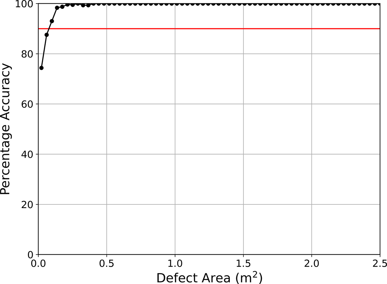
Figure 20. Accuracy versus defect area for the nine-probe results.
The regression results are tested on 4,754 samples. Table 5 shows the performance metrics (MAE, RMSE, and R 2) for the updated regressor, together with percentage improvements with respect to the results discussed in Section 3.2. It can be seen that all performance metrics improve when an additional central probe is included. Among all the output variables, the defect area and position show the greatest improvement in predictive accuracy, with 34 and 29% improvement is the MAE, respectively. Figure 21 shows the real versus predicted variable plots for all output variables. The improvement is obvious with respect to Figure 14, as all variables plot in a narrower band around the 1:1 dashed red line.
Table 5. Performance metrics and improvement (%) for regression model with nine probes
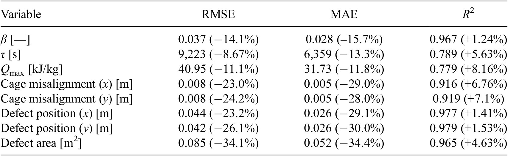
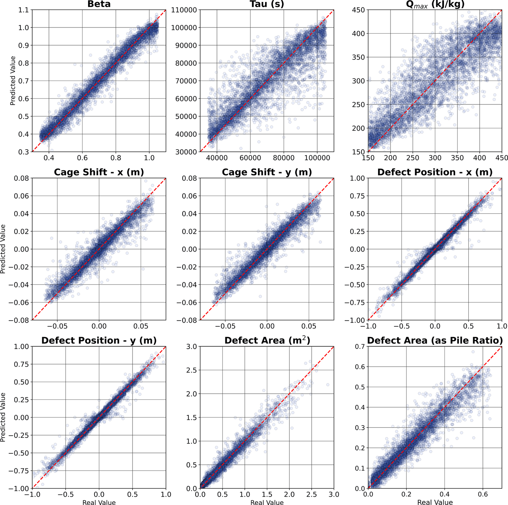
Figure 21. Correlation between real and predicted variables for the nine-probe model.
4. Conclusions
This study presents a comprehensive ML classification and regression model developed as a proof of concept to detect soil or bentonite inclusions in drilled foundations based on TIP data. The model is trained based on a conservative scenario, where a large range of variation in material properties is considered. The model’s robustness was improved by adding random noise to all temperature readings, thereby mitigating the inherent determinism of numerical FE data. The following conclusions can be drawn:
-
- The classifier can label correctly 94% of the processed samples. Thermal variations in the central section of the pile are challenging to capture due to the probes’ positioning near the edge of the pile, limiting detection capability in these regions. The overall accuracy of the model is very good ( $ {R}^2=0.935 $
).
$ {R}^2=0.935 $
). -
- The false positive rate is significantly lower than the false negative rate. False negatives are primarily associated with defects of varied sizes located within the central 25% of the pile radius. These defects remain undetected due to the considerable distance to the nearest optical fiber probes.
-
- Through regression, very high accuracies can be achieved when predicting defect size, location, and cage misalignment. Hydration parameters can also be back-calculated with reasonable precision.
-
- Including a central probe can significantly improve the ability to predict defects located close to the pile center, particularly through the reduction of false negatives in the classification stage. The inclusion of an additional probe leads to improvements across all labels, with reductions in MAE for defect location, size, and cage misalignment ranging between 28 and 35%. Therefore, it is recommended to include an additional probe if conditions allow.

This study focused on demonstrating the potential of ML techniques in TIP using data generated through 2D modeling. For greater applicability to complex structures, the model can be expanded to simulate the pile behavior in 3D, potentially covering additional defect types, such as necking, uneven radii, or internal steps. Currently, each sample with defects includes only a single circular defect. Incorporating multiple defects and/or varying their shape in future simulations may provide a more accurate representation of real-world construction scenarios.
List of abbreviations
- ANN
-
artificial neural network
- AUC
-
area under the curve
- FE
-
finite element
- HoH
-
heat of hydration
- MAE
-
mean absolute error
- ML
-
machine learning
- RMSE
-
root mean square error
- TIP
-
thermal integrity profiling
Data availability statement
The data that support the findings of this study are available in Zenodo at http://doi.org/10.5281/zenodo.14674381.
Author contribution
Javier Sánchez Fernández: Data curation (lead), formal analysis (equal), investigation (lead), methodology (lead), writing—original draft (lead), writing—review and editing (supporting).
Agustin Ruiz López: Conceptualization (equal), methodology (Supporting), supervision (equal), writing—review and editing (equal).
David M.G. Taborda: Conceptualization (equal), methodology (supporting), project administration (lead), supervision (equal), writing—review and editing (equal).
Funding statement
This work was supported by the Natural Environment Research Council [NE/S007415/1] and by the Engineering and Physical Sciences Research Council (EPSRC) through the project intigeo [EP/R511547/1].
Competing interests
The authors declare none.


 Open access
Comments
No Comments have been published for this article.