


Impact Statement
This paper investigates approaches for creating neural network models that satisfy the structure’s physical constraints and measured deflection data. It also examines the ability of the models to generalize for uniformly distributed load (UDL) conditions beyond the training data if informed of the linear relationship between UDL and deflection. The overall goal is to evaluate the improvement in predictive accuracy, specifically in the behavior of structures, when the models are trained with limited physical knowledge and then applied to new, unseen data. The ability to predict structural behavior accurately will support maintenance, repair, and optimization decisions and consequently will be valuable for the areas of structural health monitoring, digital twins, and virtual sensing.
1. Introduction
Structural health monitoring (SHM) (Figueiredo and Brownjohn, Reference Figueiredo and Brownjohn2022; Fremmelev et al., Reference Fremmelev, Ladpli, Orlowitz, Bernhammer, Mcgugan and Branner2022) is increasingly employed on civil infrastructures such as bridges for preserving their integrity and safety, and more generally for their effective maintenance and management. A key unresolved challenge is the translation of SHM data to decision-making. This requires processing vast amounts of measurement data, such as that from the Queensferry Crossing Bridge in the United Kingdom with over 2,184 sensors (Cousins et al., Reference Cousins, McAra and Hill2022), to provide actionable information to bridge operators. Over the years, several studies have focused on this challenge with an emphasis particularly on damage detection (Middleton et al., Reference Middleton, Fidler and Vardanega2016; Webb et al., Reference Webb, Vardanega and Middleton2015). Worden et al. (Reference Worden, Cross, Dervilis, Papatheou and Antoniadou2015) offered a classification of the different stages of damage identification—from anomaly detection to damage prognosis, with most studies focusing primarily on the first two stages. Increasingly, however, the emphasis has turned to preventive maintenance and long-term structural management by leveraging recent developments in AI and machine learning to generate digital twins (Sacks et al., Reference Sacks, Brilakis, Pikas, Xie and Girolami2020) that not only detect anomalous events in real time from measured data but also offer detailed insight into structural behavior and performance, such as by tracking gradual deterioration of components and estimating remaining service life.
Modeling of digital twins in the context of structural identification and damage assessment can involve three kinds of approaches. First, model-based methods, which create an accurate physics-based model—typically a finite element model (FEM), of the structure (Sohn et al., Reference Sohn, Farrar, Hemez and Czarnecki2002) by updating model parameters, based on actual observations. The updated FEM will subsequently serve as a benchmark against which new measurements will be compared for assessing the integrity and performance of the monitored structure. The drawbacks of model-based methods are that they are computationally intensive, have simplified assumptions and approximations, and are subject to uncertainties in modeling parameters (Farrar and Worden, Reference Farrar and Worden2012). Certain limitations may be addressed through uncertainty quantification analysis, as proposed by Sankararaman and Mahadevan (Reference Sankararaman and Mahadevan2013), or alternatively through probabilistic approaches like Bayesian model updating (Kamariotis et al., Reference Kamariotis, Chatzi and Straub2022).
The second class of approaches is data-driven methods. These typically rely on machine learning algorithms, primarily unsupervised learning algorithms, and detect anomalies by identifying changes to patterns in measurement data through comparisons with patterns observed during the structure’s normal operation. In full-scale structures, distinguishing between feature changes due to damage and those caused by changing operational and environmental conditions such as temperature and wind remains a challenge (Figueiredo and Brownjohn, Reference Figueiredo and Brownjohn2022). In addition, data covering a wide range of structural states are seldom available for training (Y. Ni et al., Reference Ni, Wang and Zhang2020), limiting the trained model’s performance and ability to generalize. However, compared to model-based methods, these are computationally less expensive and are easier to apply for real-time monitoring.
The third class of methods—physics-informed machine learning (PIML) methods (Karniadakis et al., Reference Karniadakis, Kevrekidis, Lu, Perdikaris, Wang and Yang2021)—are a relatively new development and are essentially machine learning algorithms that have been augmented with physics-based knowledge, provided in the form of constraints and loss function, or directly implemented in their architecture. PIML models, which can fully or partially satisfy the governing physics of a structure while being data-driven, have the potential for accurate predictions and improved generalization, defined as the model’s ability to extrapolate predictions beyond the training set into unobserved regions.
In the field of SHM, PIML approaches are conducted through physics-informed neural networks (PINNs), which adjust their loss function to incorporate physics-based constraints, ensuring adherence to the governing physics equations of structural systems, which is the focus of this paper. Additionally, hybrid models that combine physics-based methods with machine learning techniques provide a noteworthy example. Specifically, the integration of Gaussian processes (GPs) with physics-based models. The mean function of the GP is used in this approach to integrate prior physical knowledge, while the observed data are incorporated using covariance functions, as discussed in the work of Cross et al. (Reference Cross, Gibson, Jones, Pitchforth, Zhang and Rogers2022).
Another hybrid approach involves using the output from physics-based models as input for machine learning algorithms. For instance, studies by Bud et al. (Reference Bud, Nedelcu, Radu, Moldovan and Figueiredo2019, Reference Bud, Moldovan, Nedelcu, Figueiredo, Rizzo and Milazzo2023) demonstrated this method, where monitoring data reflecting normal operational conditions of an undamaged structure, along with numerical data from FEM under extreme environmental conditions or damage scenarios, are utilized to train a machine learning algorithm. For further exploration, Xu et al. (Reference Xu, Kohtz, Boakye, Gardoni and Wang2023) undertook a comprehensive review of PIML methods for reliability and system safety applications, and Karniadakis et al. (Reference Karniadakis, Kevrekidis, Lu, Perdikaris, Wang and Yang2021) discussed applications of PIML for forward and inverse problems as well as capabilities and their limitations.
The concept of PINNs is developed by Raissi et al. (Reference Raissi, Perdikaris and Karniadakis2017a,Reference Raissi, Yazdani and Karniadakisb) in a two-part article, which is consolidated into a merged version published in 2019 (Raissi et al., Reference Raissi, Perdikaris and Karniadakis2019). PINNs were introduced as a new class of data-driven solvers and as a novel approach in scientific machine learning for dealing with problems involving partial differential equations (PDEs) (Cuomo et al., Reference Cuomo, Di Cola, Giampaolo, Rozza, Raissi and Piccialli2022) using automatic differentiation. Several studies have since applied PINNs for a range of scientific problems (Shukla et al., Reference Shukla, Xu, Trask and Karniadakis2022), involving stochastic PDEs, integro-differential equations, fractional PDEs, non-linear differential equations (Uddin et al., Reference Uddin, Ganga, Asthana and Ibrahim2023), and optimal control of PDEs (Mowlavi and Nabi, Reference Mowlavi and Nabi2023). Within engineering, PINNs have been applied to problems in fluid dynamics (Mao et al., Reference Mao, Jagtap and Karniadakis2020; Raissi et al., Reference Raissi, Yazdani and Karniadakis2020; Sliwinski and Rigas, Reference Sliwinski and Rigas2023), heat transfer (Zobeiry and Humfeld, Reference Zobeiry and Humfeld2021), tensile membranes (Kabasi et al., Reference Kabasi, Marbaniang and Ghosh2023), and material behavior modeling (Zheng et al., Reference Zheng, Li, Qi, Gao, Liu and Yuan2022). However, there are only a few applications to SHM, the subject area of focus in this paper.
Previous studies on PINNs for SHM have primarily focused on training PINNs to satisfy the PDEs that govern the dynamic behavior of structural systems. Lai et al. (Reference Lai, Mylonas, Nagarajaiah and Chatzi2021) and W. Liu et al. (Reference Liu, Lai, Bacsa and Chatzi2022) investigated physics-informed neural ordinary differential equations and physics-guided deep Markov models for structural identification and tested their prediction capabilities for a series of numerical and experimental examples. Lai et al. (Reference Lai, Liu, Jian, Bacsa, Sun and Chatzi2022) presented a framework that combines physics-based modeling and deep learning techniques to model civil and mechanical dynamical systems. They showed that the generated models have the ability to effectively reconstruct the structural response using data from only a limited number of sensors, although performance was observed to deteriorate when the dynamic regime deviated significantly from the training data. P. Ni et al. (Reference Ni, Sun, Yang and Li2022) used a multi-end convolutional autoencoder to reconstruct the full seismic response of multi-degree of freedom (DOF) systems. They found that their methodology could reconstruct the seismic response of multi-DOF systems given a small training dataset, and PINNs performed better than conventional neural networks (NNs) with small datasets, particularly when the training data contained noise. Yuan et al. (Reference Yuan, Zargar, Chen, Wang, Zonta, Sohn and Huang2020) investigated the use of PINNs to solve forward and inverse PDE-based problems based on dynamic modeling of beam structures using synthetic sensor data analysis.
Further research is needed into the application of PINNs for quasi-static monitoring, which involves analyzing a structure’s response at discrete time intervals. This type of monitoring is critical for assessing the long-term monitoring of structures (Kromanis and Kripakaran, Reference Kromanis and Kripakaran2014, Reference Kromanis and Kripakaran2016). In contrast to dynamic monitoring, quasi-static monitoring frequently uses sampling rates that may not sufficiently capture vibration properties, instead focusing on static responses such as strains and displacements. PINNs, by leveraging their physics-informed nature, may be able to compensate for insufficient sampling rates by directly integrating physical laws into the learning process, enhancing the model’s ability to infer accurate responses even from limited data. This introduces other challenges such as temporally variable loading, which complicate modeling and verification of the PDE within PINNs. This study will investigate this aspect. It also leads to the other key novel contribution, which is to examine how model performance is influenced by the different physics-based constraints implemented within the loss function of a PINN. Specifically, we aim to examine whether a PINN that enforces the structure’s boundary conditions and uses sensor data from a limited number of locations across the structure can accurately model the structural system despite not explicitly incorporating the governing PDE, which can be difficult to evaluate due to variable loading. The hypothesis is that deflections from a sparse set of sensors and constraints on satisfying force boundary conditions can allow PINNs to generalize for the whole structure. The generated PINNs will also be tested for their capability to predict deflections and internal forces at locations where there are no sensors. Lastly, we will also evaluate their potential for predicting deflections and forces for loads unseen in the training datasets.
The paper uses the numerical model of a square concrete slab, representative of a building structural element, to illustrate and test the developed ideas. It states the governing PDE and the boundary conditions of the slab, and describes how these can be enforced through the loss function for a PINN. The paper then investigates the effect of the various terms in the loss function on PINN model performance through three case studies. Case Study 1, which assumes constant unchanging load, examines five different setups of PINNs, each with different loss functions incorporating varying levels of physical knowledge. Each of the PINN setups is evaluated for four measurement cases, representing increasing amounts of measurement data derived from simulated FEM analytical solution. Case Study 2 includes the applied loading as an input variable for the NNs. Case Study 3 is aimed at investigating the robustness of the PINNs to (i) deviations from idealized boundary conditions, and (ii) varying levels of noise in data. The case studies are primarily conducted in the spatial domain. Extending them to include a temporal component would pose challenges, such as the need for more complex model architectures and potentially larger datasets to effectively capture temporal dynamics.
The outline of this paper is as follows. In Section 2, the plate problem and the methodology adopted for generating PINNs are introduced. Case Study 1 and the corresponding results are discussed in Section 3. Using the results as a basis, Case Study 2 is set up and this process and the results are presented in Section 4. Section 5 is dedicated to Case Study 3, which explores additional complexities. Finally, Section 6 summarizes the key conclusions of this study.
2. Problem setup and methodology
This section outlines the structure—a typical reinforced concrete floor slab, that is to be modeled using a PINN. It describes the underlying physics of the structure and the scenarios that are considered. It then describes the structure of the PINN, its parameters and the approaches adopted for imposing the physical constraints on the PINN.
2.1. Kirchhoff–Love plate
The Kirchhoff–Love plate theory (Kirchhoff, Reference Kirchhoff1850; Love, Reference Love1888) is a mathematical model for calculating stresses and deflections in thin plates subjected to forces and moments. This model, which was first proposed by Love in 1888, is a two-dimensional extension of the Euler–Bernoulli beam theory. Kirchhoff’s assumptions provided a basis for the development of this theory. The model is employed for the analysis and design of a wide range of structural components in civil engineering including concrete slabs.
2.1.1. Governing equations
Figure 1 presents a square plate with four simply supported edges labeled A, B, C, and D. The plate is subjected to a uniformly distributed load (UDL) $ q $
across its entire surface. The magnitude of the UDL directly influences the deflections in the plate, a relationship we will attempt to capture in modeling. The vertical deflection w(x,y), that is, along the
$ q $
across its entire surface. The magnitude of the UDL directly influences the deflections in the plate, a relationship we will attempt to capture in modeling. The vertical deflection w(x,y), that is, along the $ z $
-direction, in a Kirchhoff–Love plate must satisfy the PDE (Equation (1)) below (Timoshenko and Woninowsky-Kerieger, Reference Timoshenko and Woninowsky-Kerieger1959):
$ z $
-direction, in a Kirchhoff–Love plate must satisfy the PDE (Equation (1)) below (Timoshenko and Woninowsky-Kerieger, Reference Timoshenko and Woninowsky-Kerieger1959):
 $$ \frac{\partial^4w}{\partial {x}^4}+2\;\frac{\partial^4w}{\partial {x}^2\partial {y}^2}+\frac{\partial^4w}{\partial\;{y}^4}-\frac{q}{D}=0. $$ $ D $
in Equation (1) represents the flexural rigidity of the plate and is determined from Young’s modulus (E), the plate’s thickness (h), and Poisson’s ratio
$ D $
in Equation (1) represents the flexural rigidity of the plate and is determined from Young’s modulus (E), the plate’s thickness (h), and Poisson’s ratio $ \nu $
as given below:
$ \nu $
as given below:
 $$ D=\frac{Eh^3}{12\left(1-{\nu}^2\right)}. $$

Figure 1. A simply supported plate under uniformly distributed load and its assumed distribution of sensors.
The bending moments represented by $ {M}_x $
,
$ {M}_x $
, $ {M}_y $
, and
$ {M}_y $
, and $ {M}_{xy} $
and shear forces represented by
$ {M}_{xy} $
and shear forces represented by $ {Q}_x $
and
$ {Q}_x $
and $ {Q}_y $
constitute the main internal forces within the plate structure from a structural engineer’s perspective. Computation of the bending moments is contingent upon an understanding of the deflection of the plate and knowledge of the flexural rigidity mentioned earlier. The following Equations (3)–(5) can be used to compute the moments from the deflections:
$ {Q}_y $
constitute the main internal forces within the plate structure from a structural engineer’s perspective. Computation of the bending moments is contingent upon an understanding of the deflection of the plate and knowledge of the flexural rigidity mentioned earlier. The following Equations (3)–(5) can be used to compute the moments from the deflections:
 $$ {M}_x=-D\left(\frac{\partial^2w}{\partial {x}^2}+\nu\;\frac{\partial^2w}{\partial {y}^2}\right), $$
 $$ {M}_y=-D\left(\frac{\partial^2w}{\partial {y}^2}+\nu\;\frac{\partial^2w}{\partial {x}^2}\right), $$
 $$ {M}_{xy}=-{M}_{yx}=-D\left(1-\nu \right)\frac{\partial^2w}{\partial x\partial y}. $$
2.1.2. Boundary conditions
Two types of boundary conditions—displacement and force boundary conditions—are enforced on a structure during structural analysis to model how the structure interacts with its environment (G. R. Liu and Quek, Reference Liu and Quek2014). Displacement boundary conditions define restrictions on the movement of specific points or regions of the structure. These are also referred to as essential boundary conditions as they are imposed directly on displacements, which are the main parameters in the governing equation, and ultimately result in equilibrium equations supporting the solution process when solving numerically.
Force boundary conditions define how internal forces and stresses at the boundaries relate to external forces (and moments) acting on the structure. These are also called natural boundary conditions since they are inherently derived from the displacements (G. R. Liu and Quek, Reference Liu and Quek2014). Both force and displacement boundary conditions are essentially physics-based constraints that a solution to a given plate problem, that is, a $ w\left(x,y\right) $
solution for Equation (1), must satisfy.
$ w\left(x,y\right) $
solution for Equation (1), must satisfy.
For the plate defined in Figure 1, the four edges are assumed as simple supports. This implies that there will be no displacement at its four boundaries; this constitutes its displacement boundary conditions. The simple supports also imply that the plate is allowed to rotate freely about the edges defined by $ x=0 $
,
$ x=0 $
, $ x=a $
,
$ x=a $
, $ y=0 $
, and
$ y=0 $
, and $ y=a $
; these constitute the force boundary conditions for the plate. In other words, these require that the bending moments
$ y=a $
; these constitute the force boundary conditions for the plate. In other words, these require that the bending moments $ {M}_x $
is zero along
$ {M}_x $
is zero along $ y=0 $
and
$ y=0 $
and $ y=a $
, and
$ y=a $
, and $ {M}_y $
is zero along
$ {M}_y $
is zero along $ x=0 $
and
$ x=0 $
and $ x=a $
.
$ x=a $
.
Equations (6)–(8) express these boundary conditions mathematically:
 $$ w=0\hskip0.4em \mathrm{along}\hskip0.4em x=0,\hskip0.4em x=a,y=0,\hskip0.4em \mathrm{and}\hskip0.4em y=a, $$
 $$ {M}_x=0\hskip0.4em \mathrm{along}\hskip0.4em y=0\hskip0.4em \mathrm{and}\hskip0.4em y=a, $$
 $$ {M}_y=0\hskip0.4em \mathrm{along}\hskip0.4em x=0\hskip0.4em \mathrm{and}\hskip0.4em x=a. $$
2.2. Synthetic sensor data
Since this study is about generating PINNs that emulate measured structural behavior, the plate is assumed to have sensors. We assume that displacement sensors are present at a set of locations across the surface as depicted in Figure 1. We will use data predicted at these locations by an FEM representing the slab in Figure 1 as measured data for training the PINNs. While we have assumed displacement sensors, the PINNs concept outlined in the subsequent section would also be applicable if other types of measurements such as strains and rotations were to be available. Consequently, this study is not concerned with the actual sensor types or the process of measurement. Researchers interested in sensor types, their failures, and their optimization for SHM can refer to relevant recent literature (Kechavarzi et al., Reference Kechavarzi, Soga, de Battista, Pelecanos, Elshafie and Mair2016; Middleton et al., Reference Middleton, Fidler and Vardanega2016; Wang et al., Reference Wang, Barthorpe, Wagg and Worden2022; Oncescu and Cicirello, Reference Oncescu, Cicirello, Rizzo and Milazzo2023).
The FEM was set up in the Ansys (2023) software and the simulations performed using the PyAnsys (Kaszynski et al., Reference Kaszynski, Derrick, Kaszynski, Ans, Jleonatti, Correia, Addy and Guyver2021) toolkit that enables Ansys integration with Python. The model utilized Shell Element 181, which incorporates six DOFs and conforms to the Kirchhoff–Love plate theory, for modeling plate bending behavior. The numerical model with a mesh made up of 64 elements and 80 nodes provides a detailed illustration of the structural behavior. Typical material properties for concrete slabs were adopted and are also shown in Figure 1. The UDL of 9,480 N/m2 is assumed, which is in the range of design loads in practice. Contour plots of the resulting deflections $ w $
, moments
$ w $
, moments $ {M}_x $
, and moment
$ {M}_x $
, and moment $ {M}_y $
for the plate are presented in Figure 2. Table 1 presents the predicted data from the model at the assumed sensor locations (see Figure 1); these are treated as measurements at the respective locations for the purpose of this study.
$ {M}_y $
for the plate are presented in Figure 2. Table 1 presents the predicted data from the model at the assumed sensor locations (see Figure 1); these are treated as measurements at the respective locations for the purpose of this study.
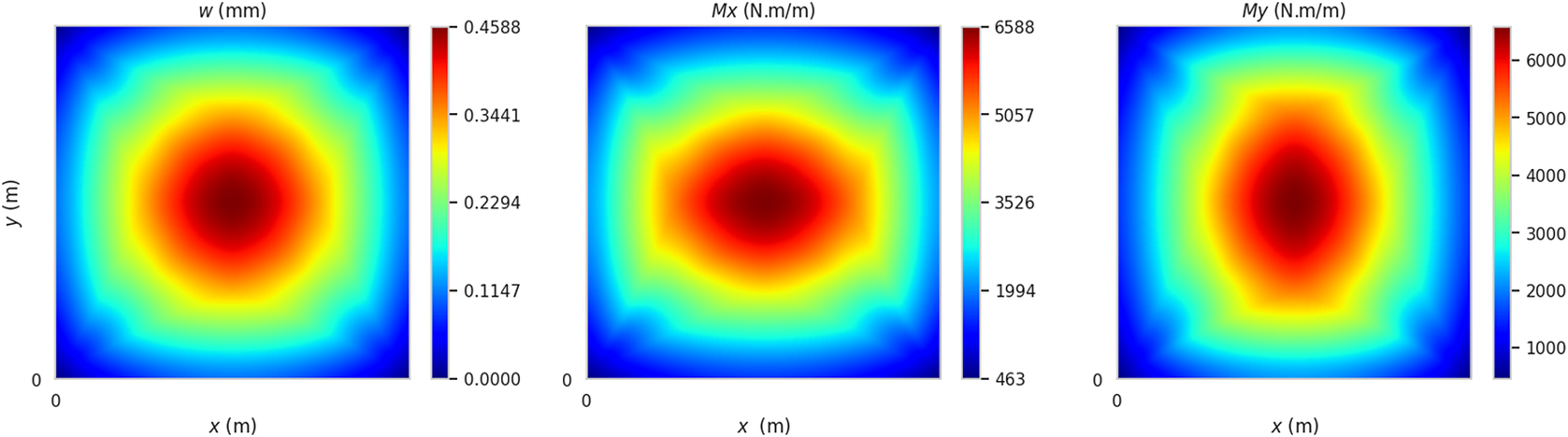
Figure 2. Deflection and moments predicted by finite element model of plate described in Figure 1.
Table 1. Summary of measured data and locations (UDL = 9,480 N/m2)

2.3. Development of PINNs
An NN denoted as a function $ NN(X) $
is shown in Equation (9). The function accepts an input variable
$ NN(X) $
is shown in Equation (9). The function accepts an input variable $ X $
, which is subjected to a series of weight matrices
$ X $
, which is subjected to a series of weight matrices $ W $
and bias vectors
$ W $
and bias vectors $ b $
to generate an output vector. The process of transformation involves the passage of input through multiple activation functions, which are represented by the
$ b $
to generate an output vector. The process of transformation involves the passage of input through multiple activation functions, which are represented by the $ \sigma $
. The incorporation of nonlinearities in this process endows the NN with the capability to discern and comprehend intricate data patterns. When the NN is used for prediction, the outcome from NN is regarded as the anticipated outcome for the system that the NN is emulating:
$ \sigma $
. The incorporation of nonlinearities in this process endows the NN with the capability to discern and comprehend intricate data patterns. When the NN is used for prediction, the outcome from NN is regarded as the anticipated outcome for the system that the NN is emulating:
 $$ NN(X)={W}_n{\sigma}_{n-1}\left({W}_{n-1}{\sigma}_{n-2}\right(\dots \left({W}_2\left({W}_1X+{b}_1\right)+{b}_{n-1}\right)+{b}_n. $$
For the plate structure, the $ x $
and
$ x $
and $ y $
coordinates, indicating the location at which the displacement is desired, constitutes the input
$ y $
coordinates, indicating the location at which the displacement is desired, constitutes the input $ X $
. The loading on the plate
$ X $
. The loading on the plate $ q $
may also be assumed as an input and the study shall explore models that accept
$ q $
may also be assumed as an input and the study shall explore models that accept $ q $
as input later in Section 4. The output from the NN is the displacement
$ q $
as input later in Section 4. The output from the NN is the displacement $ w $
. Other derived parameters such as bending moments
$ w $
. Other derived parameters such as bending moments $ {M}_x $
,
$ {M}_x $
, $ {M}_y $
, and
$ {M}_y $
, and $ {M}_{xy} $
may also be predicted using the NN as will be demonstrated later on.
$ {M}_{xy} $
may also be predicted using the NN as will be demonstrated later on.
The training of NNs typically requires the minimization of a loss function, such as the mean squared error (MSE) computed between predictions and expected results for a training dataset comprising preexisting information. In the case of PINNs, the loss function incorporates components beyond this MSE. Specifically, terms associated with the governing PDE for the system and its boundary conditions are included. In this manner, the PINN is not only able to offer accurate predictions for the training dataset but also aims to satisfy physical constraints for the system. This study models the loss function as an aggregate loss, represented as $ \mathrm{\mathcal{L}} $
, that is computed as the summation of four different loss components—
$ \mathrm{\mathcal{L}} $
, that is computed as the summation of four different loss components— $ {\mathrm{\mathcal{L}}}_f $
,
$ {\mathrm{\mathcal{L}}}_f $
, $ {\mathrm{\mathcal{L}}}_w $
,
$ {\mathrm{\mathcal{L}}}_w $
, $ {\mathrm{\mathcal{L}}}_m $
, and
$ {\mathrm{\mathcal{L}}}_m $
, and $ {\mathrm{\mathcal{L}}}_d $
, as shown in Equation (10):
$ {\mathrm{\mathcal{L}}}_d $
, as shown in Equation (10):
 $$ \mathrm{\mathcal{L}}={\mathrm{\mathcal{L}}}_f+{\mathrm{\mathcal{L}}}_w+{\mathrm{\mathcal{L}}}_m+{\mathrm{\mathcal{L}}}_d. $$ $ {\mathrm{\mathcal{L}}}_f $
,
$ {\mathrm{\mathcal{L}}}_f $
, $ {\mathrm{\mathcal{L}}}_w $
, and
$ {\mathrm{\mathcal{L}}}_w $
, and $ {\mathrm{\mathcal{L}}}_m $
evaluate how well the NN satisfies the governing PDE, the displacement boundary conditions, and the force boundary conditions, respectively.
$ {\mathrm{\mathcal{L}}}_m $
evaluate how well the NN satisfies the governing PDE, the displacement boundary conditions, and the force boundary conditions, respectively. $ {\mathrm{\mathcal{L}}}_d $
represents the performance of the NN for the training dataset. Each of these loss terms is written as the product of a weight
$ {\mathrm{\mathcal{L}}}_d $
represents the performance of the NN for the training dataset. Each of these loss terms is written as the product of a weight $ {\alpha}_i $
and the related MSE. Consequently,
$ {\alpha}_i $
and the related MSE. Consequently, $ \mathrm{\mathcal{L}} $
can be formulated as follows, wherein
$ \mathrm{\mathcal{L}} $
can be formulated as follows, wherein $ {\alpha}_f $
,
$ {\alpha}_f $
, $ {\alpha}_w $
,
$ {\alpha}_w $
, $ {\alpha}_m $
, and
$ {\alpha}_m $
, and $ {\alpha}_d $
represent the weights associated with the respective MSE values:
$ {\alpha}_d $
represent the weights associated with the respective MSE values:
 $$ \mathrm{\mathcal{L}}={\alpha}_f{MSE}_f+{\alpha}_w{MSE}_w+{\alpha}_m{MSE}_m+{\alpha}_d{MSE}_d. $$
Each of the MSE terms in Equation (11) is described in detail below.
-
1. $ {MSE}_f $
represents the average residual for the governing PDE outlined in Equation (1). The mean of the residual
$ f\left(x,y\right) $
(see Equation (12)) evaluated at a set of “collocation points” —
$ \left\{\left({x}_i,{y}_i\right):0\le i\le {N}_f\right\} $
—within the domain of the plate is taken as
$ {MSE}_f $
as shown in Equation (13). The partial derivatives will be evaluated using automatic differentiation:
$ {MSE}_f $
represents the average residual for the governing PDE outlined in Equation (1). The mean of the residual
$ f\left(x,y\right) $
(see Equation (12)) evaluated at a set of “collocation points” —
$ \left\{\left({x}_i,{y}_i\right):0\le i\le {N}_f\right\} $
—within the domain of the plate is taken as
$ {MSE}_f $
as shown in Equation (13). The partial derivatives will be evaluated using automatic differentiation:


 $$ f\left(x,y\right)=\frac{\partial^4w}{\partial {x}^4}+2\hskip0.35em \frac{\partial^4w}{\partial {x}^2\partial {y}^2}+\frac{\partial^4w}{\partial \hskip0.35em {y}^4}-\frac{q}{D}, $$
 $$ {MSE}_f=\frac{1}{N_f}\sum \limits_{i=1}^{N_f}\parallel f\left({x}_i,{y}_i\right){\parallel}^2. $$
-
2.
$ {MSE}_w $
addresses the plate’s displacement boundary conditions (Equation (6)). A set of
$ 4{N}_w $
points is generated by randomly choosing
$ {N}_w $
points from each of the four edges of the plate boundaries,resulting in a total of
$ 4{N}_w $
points given by
$ \left\{\left({x}_i,{y}_i\right):0\le i\le 4{N}_w\right\} $
. The first
$ 2{N}_w $
points are from edges AB and CD, and the last
$ 2{N}_w $
points are from edges AD and BC. We predict the displacements at these points using the PINN and compute the average error
$ {MSE}_w $
in the predictions, which should be zero to satisfy the boundary conditions, using Equation (14) below:


 $$ {MSE}_w=\frac{1}{N_w}\sum \limits_{i=1}^{N_w}\parallel w\left({x}_i,{y}_i\right){\parallel}^2. $$
-
3.
$ {MSE}_m $
is similar to
$ {MSE}_w $
but addresses the force boundary condition (Equations (7) and (8)). The same
$ {N}_w $
points used for
$ {MSE}_w $
are also employed here.
$ {MSE}_m $
is computed as given in Equation (15), wherein
$ {M}_x=0 $
is required for points along edges AD and BC, and
$ {M}_y=0 $
is required for the points along edges AB and CD. The moments, being derivatives of deflection
$ w $
(Equations (3) and (4)), are evaluated using automatic differentiation:


 $$ {MSE}_m=\frac{1}{4{N}_w}\left[\sum \limits_{i=1}^{2{N}_w}\parallel {M}_x\left({x}_i,{y}_i\right){\parallel}^2+\sum \limits_{i=2{N}_w+1}^{4{N}_w}\parallel {M}_y\Big({x}_i,{y}_i\Big){\parallel}^2\right]. $$
-
4.
$ {MSE}_d $
relates to the reconstruction of the deflection field based on measurements from a sparse sensor array. The sensor locations for the plate are presented in Figure 1. If
$ {N}_d $
sensors are employed on the plate at locations
$ \left\{\left({x}_i,{y}_i\right):0\le i\le {N}_d\right\} $
, then the measurements
$ D\left({x}_i,{y}_i\right) $
at these locations can be compared against the corresponding displacement predictions from the PINN to compute
$ {MSE}_d $
as shown below:


 $$ {MSE}_d=\frac{1}{N_d}\sum \limits_{i=1}^{N_d}\parallel D\left({x}_i,{y}_i\right)-w\left({x}_i,{y}_i\right){\parallel}^2. $$
2.4. PINN setup and tuning parameters
Figure 3 illustrates the schematic overview of the PINNs framework. The diagram depicts a feed-forward NN that is fully connected and accepts coordinates $ \left(x,y\right) $
as inputs to predict a solution
$ \left(x,y\right) $
as inputs to predict a solution $ w\left(x,y\right) $
, the expected deflection at the specified location. The technique of automatic differentiation is utilized for the computation of the derivatives of
$ w\left(x,y\right) $
, the expected deflection at the specified location. The technique of automatic differentiation is utilized for the computation of the derivatives of $ w $
in relation to the inputs. The derivatives are subsequently evaluated at specific locations and employed to find
$ w $
in relation to the inputs. The derivatives are subsequently evaluated at specific locations and employed to find $ {MSE}_f $
,
$ {MSE}_f $
, $ {MSE}_w $
,
$ {MSE}_w $
, $ {MSE}_m $
, and
$ {MSE}_m $
, and $ {MSE}_d $
as explained in Equations (13)–(16). The number of points for
$ {MSE}_d $
as explained in Equations (13)–(16). The number of points for $ {N}_f $
and
$ {N}_f $
and $ {N}_w $
is equal to 800 and 100, respectively.
$ {N}_w $
is equal to 800 and 100, respectively.

Figure 3. Schematic of the physics-informed neural networks.
Our code is based on the work of Bischof and Kraus (Reference Bischof and Kraus2022), which examined the application of PINNs to a comparable plate with the aim of achieving weight balance across the loss function terms. We have adapted their open-source code for our case studies and this can be found at GitHub. The TensorFlow (Abadi et al., Reference Abadi, Agarwal, Barham, Brevdo, Chen, Citro, Corrado, Davis, Dean, Devin, Ghemawat, Goodfellow, Harp, Irving, Isard, Jozefowicz, Jia, Kaiser, Kudlur, Levenberg, Mane, Monga, Moore, Murray, Olah, Schuster, Shlens, Steiner, Sutskever, Talwar, Tucker, Vanhoucke, Vasudevan, Viegas, Vinyals, Warden, Wattenberg, Wicke, Yu and Zheng2015) library is used to implement this computational process, and the model is trained on Google Colab, with GPU capabilities.
Table 2 provides a detailed summary of the hyperparameters that were selected for the PINN model. These hyperparameters were carefully optimized through a series of iterative trial and error processes to achieve the best possible performance of the model. The learning rate, an essential parameter that governs the magnitude of the step taken during each iteration during the minimization of the loss function, is set as 0.001. The architecture of the NN employed in this study consists of four hidden layers, each containing 64 neurons. This configuration is selected after examining various architectures, ranging from two to six hidden layers. The choice of four hidden layers attains a balance aimed at reducing computational time and avoiding over-fitting. Additionally, the Tanh activation function is employed in each layer. The Tanh function is chosen due to its non-linear characteristics, which are essential for PINNs. Unlike linear activation functions, such as ReLU, Tanh enhances the network’s ability to learn and predict nonlinear patterns. This is a key requirement in the framework of PINNs, where handling derivative terms in the governing equations is crucial for accurate prediction and pattern acquisition. The model is subjected to a training process spanning 1,500 epochs, where each epoch involves a complete iteration over the entire training dataset. The optimizer utilized is Adam. Further techniques for enhancing the model’s efficacy include (i) early stopping, which halts the training process as soon as the model’s performance begins to deteriorate on a validation dataset, thus preventing overfitting, and (ii) ReduceLROnPlateau, which limits the learning rate when the model’s learning advancement decelerates, enabling more precise calibration (Goodfellow et al., Reference Goodfellow, Bengio and Courville2016).
Table 2. Hyperparameters related to the neural network’s architecture and training

2.5. Methods for functional loss balancing $ {MSE}_f $
,
$ {MSE}_f $
, $ {MSE}_w $
,
$ {MSE}_w $
, $ {MSE}_m $
, and
$ {MSE}_m $
, and $ {MSE}_d $
are based on different measurement units, and their magnitudes may vary by multiple orders of magnitude. Consequently, the overall loss
$ {MSE}_d $
are based on different measurement units, and their magnitudes may vary by multiple orders of magnitude. Consequently, the overall loss $ \mathrm{\mathcal{L}} $
may be biased toward one of these loss terms if these are simply added up. To avoid this, we employ weights—
$ \mathrm{\mathcal{L}} $
may be biased toward one of these loss terms if these are simply added up. To avoid this, we employ weights— $ {\alpha}_f $
,
$ {\alpha}_f $
, $ {\alpha}_w $
,
$ {\alpha}_w $
, $ {\alpha}_m $
, and
$ {\alpha}_m $
, and $ {\alpha}_d $
, as already stated in Equation (11).
$ {\alpha}_d $
, as already stated in Equation (11).
The gradient descent algorithm is chosen to determine the optimal weights for the various terms in the loss function. The algorithm considers the relative importance of each term in the loss function and avoids overemphasizing any one term by setting the sum of the weights to 1. This method is effective at determining the optimal weights for each term of the loss function, allowing us to train the model more efficiently and accurately. Figure 4 shows the contribution of loss function components with respect to the total loss and median of the log MSE $ \left({L}_2\right) $
loss during optimization. The loss decreases rapidly at the start of optimization as expected but slows after 400 epochs. After that, due to convergence of solution, the loss decreases very slowly.
$ \left({L}_2\right) $
loss during optimization. The loss decreases rapidly at the start of optimization as expected but slows after 400 epochs. After that, due to convergence of solution, the loss decreases very slowly.

Figure 4. (a) Percentage contribution of loss components. (b) Loss optimization observed with gradient descent.
2.6. Optimizing the number of collocation points
Collocation points are specialized samples in a computational domain that have been selected to embed physical laws into the network with the objective of proving computational simplicity for efficient evaluation, representatives to cover the computational domain, and feasibility, which ensures the points represent attainable system states or domains (Sholokhov et al., Reference Sholokhov, Liu, Mansour and Nabi2023). As consequently, selecting an appropriate set of collocation points not only improves model precision during PINNs training, ensuring that the NN learns to adhere to the governing physical principles of the system being modeled, but also reduces computational time. This investigation is divided into two distinct but interconnected sections: the examination of the influence on model performance of the number of collocation points within the model’s internal domain and those located around its boundaries.
For internal domain, we initially focus on the number of collocation points ranging from 400 to 1,000. The number of boundary collocation points along the plate edges is fixed at 50 per edge. For each collocation point setting, PINNs are trained with 10 different seeds. These seeds are randomized for each setup, which means that the model is trained 10 times with 10 different, randomly chosen initial seeds for producing robust statistical metrics for each specific number of collocation points (400, 500, up to 1,000). Figure 5a,b shows the box plots of the root-mean-square error (RMSE) associated with deflection and bending moments (Mx), respectively. According to the analysis, the relationship between the number of internal domain collocation points and RMSE does not always follow a strictly linear or decreasing trend. In Figure 5a, while the RMSE for deflection generally decreases as the number of collocation points increases, there are notable exceptions to this pattern, particularly at points ranging from 600 to 900. These examples show that increasing the number of collocation points does not always result in improved model accuracy for deflection predictions. Figure 5b, on the other hand, shows a somewhat more consistent trend for the RMSE associated with Mx, though it, too, exhibits fluctuations, emphasizing the complexities of the relationship between collocation points and model accuracy. Remarkably, the variance in RMSE tends to narrow at higher collocation points (specifically, 800 and 900), implying that model performance at these levels is more stable and consistent.

Figure 5. (a) Deflection root-mean-square (RMSE) and (b) moment RMSE for different numbers of internal domain collocation points.
The influence of boundary collocation points on model performance is subsequently investigated. The number of internal collocation points is now fixed at 800, as identified in the previous stage. Six different counts of boundary collocation points ranging from 50 to 100 per edge (i.e., 200 to 400 in total), while adhering to the analytical methodology established for the internal domain. Figure 6a,b shows the RMSE values for the chosen number of boundary points. Figure 6a shows that the RMSE for deflection increases as the number of boundary collocation points increases, with the lowest RMSE observed at the fewest number of boundary points. Despite this trend, the RMSE variance tends to narrow in the range of 80 to 100 points per edge, indicating that model performance may stabilize at higher collocation point counts. Figure 6b, on the other hand, shows a different pattern for the RMSE associated with moment (Mx), where a decrease in RMSE values is observed as the number of collocation points increases. The best and most consistent RMSE values are found between 70 and 90 points per edge. Based on the analysis presented here, the study proceeds with 800 collocation points within the internal domain, which is supplemented with 400 points around the boundaries.

Figure 6. (a) Deflection root-mean-square (RMSE) and (b) moment RMSE for different numbers of boundary collocation points.
3. Case Study 1
In this section, the UDL $ q $
is assumed to be constant for the duration of monitoring. The study then evaluates the influence of the loss terms—
$ q $
is assumed to be constant for the duration of monitoring. The study then evaluates the influence of the loss terms— $ {\mathrm{\mathcal{L}}}_f $
,
$ {\mathrm{\mathcal{L}}}_f $
, $ {\mathrm{\mathcal{L}}}_w $
,
$ {\mathrm{\mathcal{L}}}_w $
, $ {\mathrm{\mathcal{L}}}_m $
, and
$ {\mathrm{\mathcal{L}}}_m $
, and $ {\mathrm{\mathcal{L}}}_d $
as given in Equation (10), on PINN performance. For this purpose, PINN models are generated for various combinations of loss terms—specifically the five scenarios, as listed in Table 3. In SN1, the loss function only includes
$ {\mathrm{\mathcal{L}}}_d $
as given in Equation (10), on PINN performance. For this purpose, PINN models are generated for various combinations of loss terms—specifically the five scenarios, as listed in Table 3. In SN1, the loss function only includes $ {\mathrm{\mathcal{L}}}_d $
, which represents the fit to the measured data. In SN2 and SN3 scenarios, displacement and force boundary conditions, respectively, are included alongside
$ {\mathrm{\mathcal{L}}}_d $
, which represents the fit to the measured data. In SN2 and SN3 scenarios, displacement and force boundary conditions, respectively, are included alongside $ {\mathrm{\mathcal{L}}}_d $
. Scenario SN4 refers to a PINN generated with a loss function combining loss terms for force and displacement boundary conditions—
$ {\mathrm{\mathcal{L}}}_d $
. Scenario SN4 refers to a PINN generated with a loss function combining loss terms for force and displacement boundary conditions— $ {\mathrm{\mathcal{L}}}_m $
and
$ {\mathrm{\mathcal{L}}}_m $
and $ {\mathrm{\mathcal{L}}}_w $
, with
$ {\mathrm{\mathcal{L}}}_w $
, with $ {\mathrm{\mathcal{L}}}_d $
. Scenario SN5 represents the case when the loss
$ {\mathrm{\mathcal{L}}}_d $
. Scenario SN5 represents the case when the loss $ {\mathrm{\mathcal{L}}}_f $
—corresponding to the satisfaction of the governing PDE, is also included.
$ {\mathrm{\mathcal{L}}}_f $
—corresponding to the satisfaction of the governing PDE, is also included.
Table 3. Summary of the loss function scenarios employed in the study

For each of the scenarios in Table 3, the study also evaluates the influence of the quantity of measurements on model performance. For this, PINN models are generated for varying number of assumed sensors (i.e., measurements)—from zero to nine, as shown by the four cases in Table 4. The case with no measurements is employed only with loss scenarios SN2–SN5 to evaluate whether enforcing constraints on governing PDE and/or boundary conditions, without having measurements, would lead to an accurate PINN.
Table 4. Summary of the measurement cases used in the study

3.1. Error metrics
The performance of the PINNs generated for the various scenarios is evaluated using multiple metrics. The RMSE given in Equation (17) captures the average magnitude of the errors between predicted and observed values, thereby providing a scale-dependent snapshot of the model’s general accuracy. The coefficient of variation (CV) of the RMSE from Equation (18) provides a scale-independent perspective by normalizing the RMSE relative to the mean of the observed values. This enables a more careful comparison of model performance across various scenarios, which is particularly useful when dealing with structures or conditions that vary in size. Lastly, the normalized mean bias error (NMBE) in Equation (19) is used to evaluate the model’s tendency for systematic bias, such as consistent overestimation or underestimation. These are computed by comparing PINN predictions against the results from the FEM (see Section 2), which is taken as the exact solution to the modeled plate. The comparison is performed at $ n=13 $
locations. Nine of the locations are the same as the locations where sensors are assumed to be present; the coordinates for these are given in Table 2. The coordinates for the other four locations are:
$ n=13 $
locations. Nine of the locations are the same as the locations where sensors are assumed to be present; the coordinates for these are given in Table 2. The coordinates for the other four locations are: $ \left(\mathrm{2.0,3.5}\right),\left(\mathrm{3.5,2.0}\right),\left(\mathrm{2.0,0.5}\right),\left(\mathrm{0.5,2.0}\right) $
:
$ \left(\mathrm{2.0,3.5}\right),\left(\mathrm{3.5,2.0}\right),\left(\mathrm{2.0,0.5}\right),\left(\mathrm{0.5,2.0}\right) $
:
 $$ RMSE=\sqrt{\frac{1}{n}\sum \limits_{i=1}^n{\left({Measurements}_i- Model\hskip0.35em {predictions}_i\right)}^2}, $$
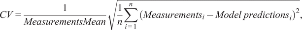 $$ CV=\frac{1}{ Measurements Mean}\sqrt{\frac{1}{n}\sum \limits_{i=1}^n{\left({Measurements}_i- Model\hskip0.35em {predictions}_i\right)}^2}, $$
 $$ NMBE=\frac{\sum_{i=1}^n(Model\hskip0.35em {predictions}_i-{Measurements}_i)}{\sum_{i=1}^n({Measurements}_i)}. $$
3.2. Results and discussion
PINNs are trained for each of the scenarios described in Section 3, and the performance of the trained models are evaluated. Table 5 shows the results obtained for the different scenarios. The performance of the PINNs are compared in terms of various parameters such as training time and loss as well as RMSE, CV, and NMBE with respect to $ w $
,
$ w $
, $ {M}_x $
, and
$ {M}_x $
, and $ {M}_y $
. Several observations can be made from the presented results.
$ {M}_y $
. Several observations can be made from the presented results.
Table 5. Error metric results for the various scenarios in Case Study 1

The general trend is that the model performance improves as the loss function includes more terms to impose increasing number of physics-based constraints, that is, as one moves from SN1 to SN5. However, the training time tends to increase, with a notably steep increase for the loss function that also requires satisfaction of the governing PDE. For each of the loss function scenarios—namely SN1–SN5, performance is observed to improve with inclusion of more measurements. This is clearly as per expectations.
SN1, which represents a regular NN trained only using measurements, shows poor performance, which is in line with expectations. The training times for these models range roughly between 1 and 4 minutes. The loss values are all extremely small indicating that the model predicts accurately at the sensor locations used for model training. The RMSE for $ w $
varies significantly with the number of measurements used for training, with a value of 1.938 mm for Case 1 but reducing to 0.0219 mm for Case 3. The CV and NMBE for w also improve with increasing number of measurements. However, the RMSE, CV, and NMBE for
$ w $
varies significantly with the number of measurements used for training, with a value of 1.938 mm for Case 1 but reducing to 0.0219 mm for Case 3. The CV and NMBE for w also improve with increasing number of measurements. However, the RMSE, CV, and NMBE for $ {M}_x $
and
$ {M}_x $
and $ {M}_y $
are excessively high, indicating a high level of variability and bias for these parameters.
$ {M}_y $
are excessively high, indicating a high level of variability and bias for these parameters.
SN2 is similar to SN1 but includes displacement boundary conditions, which essentially implies additional training data points across the four edges of the plate. When compared to SN1, models for SN2 offer more accurate predictions for displacements and moments. Training times are roughly 5 minutes with loss values that are marginally higher than for SN1. RMSE and CV for $ w $
are generally consistent and not varying as dramatically as in SN1. Predictions for
$ w $
are generally consistent and not varying as dramatically as in SN1. Predictions for $ {M}_x $
and
$ {M}_x $
and $ {M}_y $
are better compared to SN1, but the errors, as indicated by RMSE, CV, and NMBE, are all still large; consequently, SN2 models are not usable for reliably predicting these parameters.
$ {M}_y $
are better compared to SN1, but the errors, as indicated by RMSE, CV, and NMBE, are all still large; consequently, SN2 models are not usable for reliably predicting these parameters.
SN3 represents the scenario where the loss function is based on the errors in predicting $ w $
at the sensor locations as well as the errors in satisfying force boundary conditions. However, unlike SN2, displacement boundary conditions are not modeled. The training times for this model are similar to SN2, and the loss values are only slightly higher. However, when compared to models for SN1 and SN2, the predictions for
$ w $
at the sensor locations as well as the errors in satisfying force boundary conditions. However, unlike SN2, displacement boundary conditions are not modeled. The training times for this model are similar to SN2, and the loss values are only slightly higher. However, when compared to models for SN1 and SN2, the predictions for $ w $
are less accurate as evident in the corresponding RMSE, CV, and NMBE metrics. In contrast,
$ w $
are less accurate as evident in the corresponding RMSE, CV, and NMBE metrics. In contrast, $ {M}_x $
and
$ {M}_x $
and $ {M}_y $
are predicted more accurately with the corresponding error metrics being more consistent and balanced, indicating improved reliability and precision.
$ {M}_y $
are predicted more accurately with the corresponding error metrics being more consistent and balanced, indicating improved reliability and precision.
SN4 brings together the features in SN1–SN3. It incorporates displacement and force boundary conditions, which are important factors in physical structure behavior. However, the governing PDE is not included in the learning process of SN4; the expectation is that the monitoring data can overcome this limitation. The results demonstrate that the models become more accurate with increasing number of measurements. All metrics—RMSE, CV, and NMBE, for the three predicted parameters $ w $
,
$ w $
, $ {M}_x $
, and
$ {M}_x $
, and $ {M}_y $
show improvement with increasing number of measurements, with results particularly for
$ {M}_y $
show improvement with increasing number of measurements, with results particularly for $ {M}_x $
and
$ {M}_x $
and $ {M}_y $
significantly more accurate compared to predictions obtained using models from the earlier scenarios. Furthermore, the time required for training is only slightly more than the time needed for SN2 and SN3, while the overall loss is similar.
$ {M}_y $
significantly more accurate compared to predictions obtained using models from the earlier scenarios. Furthermore, the time required for training is only slightly more than the time needed for SN2 and SN3, while the overall loss is similar.
Scenario SN5 builds on SN4 by incorporating the loss term for satisfying the governing PDE. These models have the longest training time (up to 2 hours 20 minutes), but also produce the best results. The error metrics are noticeably more stable and consistent compared to the previous scenarios. For example, this has the lowest CV for deflection $ w $
. Models also offer good prediction accuracy for the moments
$ w $
. Models also offer good prediction accuracy for the moments $ {M}_x $
and
$ {M}_x $
and $ {M}_y $
. Overall, SN5 models perform with the least amount of error and bias, and generally offer the most accurate predictions among the five models.
$ {M}_y $
. Overall, SN5 models perform with the least amount of error and bias, and generally offer the most accurate predictions among the five models.
Models from SN3–SN5 offer significantly better performance than SN1 and SN2, particularly for Case 3, which has the most number of measurements. Consequently, we explore the generalization capability of these models in more detail. Tables 6 and 7 show the contour plots for $ w $
and
$ w $
and $ {M}_x $
and
$ {M}_x $
and $ {M}_y $
, respectively. The plots in these tables need to be compared with the contours from finite element analysis given in Figure 2. Notably, despite the omission of governing equations during the learning process, SN4 yields promising results. This is possibly due to the monitoring data, particularly with more sensors offering improved spatial coverage and hence being able to compensate for the lack of the loss term requiring satisfaction of the governing PDE. Consequently, SN4 may offer a simplified learning model that combines the advantages of both physical knowledge and data-driven learning, while being computationally modest. We will explore this further in the next section, where we focus primarily on how the learning model in SN4 can be adapted for scenarios where the loading is also allowed to vary.
$ {M}_y $
, respectively. The plots in these tables need to be compared with the contours from finite element analysis given in Figure 2. Notably, despite the omission of governing equations during the learning process, SN4 yields promising results. This is possibly due to the monitoring data, particularly with more sensors offering improved spatial coverage and hence being able to compensate for the lack of the loss term requiring satisfaction of the governing PDE. Consequently, SN4 may offer a simplified learning model that combines the advantages of both physical knowledge and data-driven learning, while being computationally modest. We will explore this further in the next section, where we focus primarily on how the learning model in SN4 can be adapted for scenarios where the loading is also allowed to vary.
Table 6. Deflection predictions of physics-informed neural networks for Case Study 1

Table 7. Moment predictions ( $ {M}_x $
) of physics-informed neural networks for Case Study 1
$ {M}_x $
) of physics-informed neural networks for Case Study 1

4. Case Study 2
To predict for different UDL conditions, we modify the PINN to accept the load as an additional input. This shift toward considering UDL as an additional input closely reflects real-world scenarios where the measured data are often obtained under varying load conditions. Implicitly, the premise is that the load is known, which is appropriate for practical monitoring scenarios.
To ensure the accuracy and robustness of the modified PINN’s predictive capabilities, a loss term that imposes a constraint on how loading and deflection are related is incorporated into the existing loss function. In this study, a simple linear relationship between load and displacement is assumed; this implies that the second derivative of displacement with respect to load should ideally equal zero. This linear relationship is a fundamental assumption in numerous areas of structural analysis and engineering. Equation (20) shows the implementation of this loss. The loss is evaluated at a set of $ {N}_q $
points, wherein
$ {N}_q $
points, wherein $ {N}_q $
is 278, 486, and 702, for Cases 1–3, respectively. These data represent deflection measurements for a total of 54 different load cases, spanning a range of 0 to 400 KN/m2. It is noted that UDL values beyond 10 KN/m2 are unrealistic but are used here solely to evaluate the generalization capability of the PINN models:
$ {N}_q $
is 278, 486, and 702, for Cases 1–3, respectively. These data represent deflection measurements for a total of 54 different load cases, spanning a range of 0 to 400 KN/m2. It is noted that UDL values beyond 10 KN/m2 are unrealistic but are used here solely to evaluate the generalization capability of the PINN models:
 $$ {MSE}_q=\frac{1}{N_q}\sum \limits_{i=1}^{N_q}\parallel \frac{\partial^2w}{\partial {q}^2}\left({x}_i,{y}_i,{q}_i\right){\parallel}^2. $$
The total modified loss function is shown in Equation (21):
 $$ \mathrm{\mathcal{L}}={\alpha}_w{MSE}_w\hskip0.35em +\hskip0.35em {\alpha}_m{MSE}_m+{\alpha}_d{MSE}_d+{\alpha}_q{MSE}_q. $$
The schematic in Figure 7 illustrates the NN’s architecture modified to incorporate UDL as an additional input. The same PINN hyperparameters referenced in Table 2 are used with one notable exception. The number of epochs was increased to 50,000 to enhance prediction accuracy. However, it was observed that the early stopping mechanism typically activated between 20,000 and 30,000 epochs, thereby preventing potential over-fitting while ensuring model efficiency.

Figure 7. Physics-informed neural networks setup for predicting response to varying uniformly distributed load.
4.1. Impact of varying UDL on PINNs’ predictions
Results for this PINN setup are given in Table 8, which sheds light on the performance of the trained PINNs for varying UDL conditions. To begin with, the predictive accuracy improves from Case 1 to Case 3, as evidenced by decreasing RMSE values for deflection and bending moments. For example, at a UDL of $ 150\;\mathrm{KN}/{\mathrm{m}}^2 $
, the RMSE drops from 0.2741 mm in Case 1 to 0.1211 mm in Case 3. This decrease in RMSE can be attributed to the increased number of points
$ 150\;\mathrm{KN}/{\mathrm{m}}^2 $
, the RMSE drops from 0.2741 mm in Case 1 to 0.1211 mm in Case 3. This decrease in RMSE can be attributed to the increased number of points $ {N}_q $
used for evaluating the loss function in each subsequent case, demonstrating that more comprehensive training data improve the model’s effectiveness.
$ {N}_q $
used for evaluating the loss function in each subsequent case, demonstrating that more comprehensive training data improve the model’s effectiveness.
Table 8. Error metric results for Case Study 2 with varying uniformly distributed load

Turning to the error metrics, RMSE and CV offer distinct but complementary perspectives on model performance. While RMSE provides an absolute measure of the prediction errors, CV normalizes these errors relative to the magnitude of the quantities being predicted. Consider the RMSE for deflection at a UDL of 150 KN/m2 in Case 3, which is 0.1211 mm, and compare it with the deflection RMSE at a UDL of 550 KN/m2 for the same case, which is 0.4608 mm. The RMSE increases as the load increases, but this is expected since the deflections themselves are larger under higher loads. The true strength of the model becomes apparent when considering the CV, which remains relatively stable (3.81%–3.95% for 150–550 KN/m2) across these conditions. The CV helps to contextualize the RMSE by indicating that the percentage error in the predictions remains consistent, even as the load increases. Interestingly, the NMBE shows both positive and negative values (less than $ \pm 7\% $
), indicating that the model’s predictions are neither consistently overestimated nor underestimated. This suggests that the additional loss term,
$ \pm 7\% $
), indicating that the model’s predictions are neither consistently overestimated nor underestimated. This suggests that the additional loss term, $ {MSE}_q $
, aimed at ensuring a realistic relationship between load and deflection, is effective in mitigating systemic bias.
$ {MSE}_q $
, aimed at ensuring a realistic relationship between load and deflection, is effective in mitigating systemic bias.
The performance of the model can also be understood through a careful analysis of the bending moment predictions, $ {M}_x $
and
$ {M}_x $
and $ {M}_y $
. Taking Case 3 as an example, the RMSE for
$ {M}_y $
. Taking Case 3 as an example, the RMSE for $ {M}_x $
is 8,478 N.m/m with a CV of 15.47% and the RMSE for
$ {M}_x $
is 8,478 N.m/m with a CV of 15.47% and the RMSE for $ {M}_y $
is 8,302 N.m/m with a CV of 15.15% when the UDL is 150 KN/m2. In the same Case 3, the RMSE for
$ {M}_y $
is 8,302 N.m/m with a CV of 15.15% when the UDL is 150 KN/m2. In the same Case 3, the RMSE for $ {M}_x $
rises to 55,186 N.m/m and the RMSE for
$ {M}_x $
rises to 55,186 N.m/m and the RMSE for $ {M}_y $
to 53,991 N.m/m for a higher UDL of 550 KN/m2, while the CV for
$ {M}_y $
to 53,991 N.m/m for a higher UDL of 550 KN/m2, while the CV for $ {M}_x $
is 25.18% and for
$ {M}_x $
is 25.18% and for $ {M}_y $
it is 24.63%. The CV is thus an important indicator here, showing that the RMSE values are rising, but only in a proportional fashion to the rising bending moment magnitudes. This is further corroborated by the NMBE, which for
$ {M}_y $
it is 24.63%. The CV is thus an important indicator here, showing that the RMSE values are rising, but only in a proportional fashion to the rising bending moment magnitudes. This is further corroborated by the NMBE, which for $ {M}_x $
is 6.15% at 150 KN/m2 and 14.83% at 550 KN/m2. Similarly, for
$ {M}_x $
is 6.15% at 150 KN/m2 and 14.83% at 550 KN/m2. Similarly, for $ {M}_y $
, the NMBE is 6.14% at 150 KN/m2 and 14.78% at 550 KN/m2. These NMBE values suggest that the model maintains a relatively consistent bias across different loading scenarios.
$ {M}_y $
, the NMBE is 6.14% at 150 KN/m2 and 14.78% at 550 KN/m2. These NMBE values suggest that the model maintains a relatively consistent bias across different loading scenarios.
Overall, this case study demonstrates the reliability of the PINN models for predicting floor slab behavior under varying loads. Remarkably, they also exhibit strong predictive capabilities for inputs beyond the range of training data, making it highly applicable for real-world SHM scenarios.
5. Case Study 3
This case study aims to explore the robustness of PINNs to uncertainties in modeling and measurement data. In structural engineering, connections are usually idealized as fully fixed or pinned for design purposes. These idealized assumptions, while often conservative from a design perspective, may not be appropriate when interpreting measurements from real structures. Real-world connections tend to be semi-rigid, that is, with partially fixity with stiffness somewhere between a fully fixed connection and a pinned connection. The semi-rigid behavior could arise from imperfections in connections, for example, due to aging materials, but typically is a direct consequence of the way the connection is fabricated, as, for example, in the case of beam–column connections and truss element connections, which are commonly assumed to be perfectly pinned for modeling but research indicates that partial fixity is more realistic representation of their behavior (Kartal et al., Reference Kartal, Basaga, Bayraktar and Muvafık2010). Consequently, PINN models that are employed to interpret measurements from real-world conditions must be capable of handling deviations from idealized assumptions on boundary conditions. We evaluate this capability through simulated measurement data obtained from the FEM implementing semi-rigid connections along the plate boundaries.
SHM data are also subject to a degree of noise. Noise can be attributed to a range of environmental and operational issues, including but not limited to changes in temperature, live load variations, and inaccuracies in sensor measurements. To replicate this characteristic, we incorporate white Gaussian white noise into our simulated SHM data. The incorporation of this noise is intended to enhance the fidelity of the synthetic data, making it more reflective of the challenges engineers would face when analyzing SHM data collected in real-world scenarios. This case study thus considers two additional layers of complexity, namely semi-rigid connections and data affected by noise. Our aim is to evaluate the adaptability and performance of PINNs in two scenarios: with and without the presence of the PDEs that govern the system.
5.1. Synthetic semi-rigid connections data
The FEM of the plate used in Case Studies 1 and 2 is modified to emulate semi-rigid connections along its edges. The initial setup parameters for load distribution, geometric dimensions, and material properties are the same as defined in Section 2.2. However, specialized connection elements—Combin14 elements that serve as torsional springs (Ansys, 2023)—are employed to simulate semi-rigid behavior. These elements will offer restraint for rotation about the plate boundary. The stiffness ( $ K\Big) $
of the elements determines the degree of restraint with 0 representing a perfectly pinned connection and very large values offering fully fixed behavior. For the purposes of this case study, a stiffness value of
$ K\Big) $
of the elements determines the degree of restraint with 0 representing a perfectly pinned connection and very large values offering fully fixed behavior. For the purposes of this case study, a stiffness value of $ \mathrm{8,261,458}\hskip0.1em \mathrm{N}\cdot \mathrm{m} $
was chosen. This value is derived from theoretical calculations assuming a reinforced concrete beam having dimensions
$ \mathrm{8,261,458}\hskip0.1em \mathrm{N}\cdot \mathrm{m} $
was chosen. This value is derived from theoretical calculations assuming a reinforced concrete beam having dimensions $ 300\hskip0.1em \times 400\hskip0.1em \mathrm{mm} $
exists along the plate boundaries, as may be the case in a building floor. Table 9 provides a summary of the number and locations of these synthetic torsional springs.
$ 300\hskip0.1em \times 400\hskip0.1em \mathrm{mm} $
exists along the plate boundaries, as may be the case in a building floor. Table 9 provides a summary of the number and locations of these synthetic torsional springs.
Table 9. Predictions from finite element model incorporating semi-rigid connection behavior along plate edges

5.2. PINNs under varying signal-to-noise ratios
The purpose of this section is to evaluate the performance of PINNs under various noise levels evaluated in terms of signal-to-noise ratios (SNRs). White Gaussian noise is incorporated into the deflection data predicted by the FE model and presented in Table 9. The noisy data $ {w}_{\mathrm{noise}} $
are formulated as in Equation (22)):
$ {w}_{\mathrm{noise}} $
are formulated as in Equation (22)):
 $$ {w}_{\mathrm{noise}}\hskip0.35em =\hskip0.35em w+\mathcal{N}\left(0,{\sigma}^2\right). $$
Here, $ w $
represents the actual displacement acquired from the FEM, and
$ w $
represents the actual displacement acquired from the FEM, and $ \mathcal{N}\left(0,{\sigma}^2\right) $
signifies white Gaussian noise with zero mean and a standard deviation
$ \mathcal{N}\left(0,{\sigma}^2\right) $
signifies white Gaussian noise with zero mean and a standard deviation $ \sigma $
determined by the desired SNR. The SNR in decibels (dB) is expressed as in Equation (23)):
$ \sigma $
determined by the desired SNR. The SNR in decibels (dB) is expressed as in Equation (23)):
 $$ SNR(dB)=10\;{\log}_{10}\left(\frac{\mathrm{Signal}\ \mathrm{Power}}{\mathrm{Noise}\ \mathrm{Power}}\right). $$
Four different SNRs are considered: 10, 20, 30, and 40 dB as presented in Figure 8. A lower SNR such as 10 dB implies a high level of noise, posing a significant challenge for any predictive model. Conversely, a higher SNR like 40 dB indicates a minimal effect of noise.

Figure 8. Effect of signal-to-noise ratio on the quality of deflection $ {w}_{\mathrm{noise}} $
data.
$ {w}_{\mathrm{noise}} $
data.
5.3. Results and discussion
PINNs are trained under two distinct scenarios: SN4, which excludes PDEs, and SN5, which incorporates them. The efficacy of these trained models is evaluated across a range of SNRs. Table 10 gives the outcomes for both scenarios, employing multiple error metrics, as already done in Case Study 1, for the predicted parameters $ w $
,
$ w $
, $ {M}_x $
, and
$ {M}_x $
, and $ {M}_y $
. The data yield several key insights.
$ {M}_y $
. The data yield several key insights.
Table 10. Error metrics for the Case Study 3 scenarios

For the SN4 scenario, the results reveal that the model accuracy improves as the noise level decreases. All error metrics exhibit an improvement trend with diminishing noise for the three parameters $ w $
,
$ w $
, $ {M}_x $
, and
$ {M}_x $
, and $ {M}_y $
. Specifically, the CV decreases from 26.87% at a 10 dB SNR to 4.11% with clean data. However, the moments
$ {M}_y $
. Specifically, the CV decreases from 26.87% at a 10 dB SNR to 4.11% with clean data. However, the moments $ {M}_x $
and
$ {M}_x $
and $ {M}_y $
are more sensitive to noise compared to deflection. For instance, the RMSE nearly doubles when the SNR changes from 40 to 10 dB. The deflection NMBE generally remains within a
$ {M}_y $
are more sensitive to noise compared to deflection. For instance, the RMSE nearly doubles when the SNR changes from 40 to 10 dB. The deflection NMBE generally remains within a $ \pm 10\% $
range and is mostly positive, indicating underestimation compared to the measured data. This suggests that the PINNs in SN4 provide a robust generalization, even when faced with substantial noise. The NMBE for
$ \pm 10\% $
range and is mostly positive, indicating underestimation compared to the measured data. This suggests that the PINNs in SN4 provide a robust generalization, even when faced with substantial noise. The NMBE for $ {M}_x $
and
$ {M}_x $
and $ {M}_y $
follows the same trend as deflection, with values reaching up to
$ {M}_y $
follows the same trend as deflection, with values reaching up to $ 33\% $
.
$ 33\% $
.
In the SN5 scenario, the models outperform those in SN4, even in noisier conditions. The CV for deflection ranges from just below 6% to 15% for clean data and a 10 dB SNR, respectively. The moments $ {M}_x $
and
$ {M}_x $
and $ {M}_y $
are less affected by noise in SN5 compared to SN4. For instance, the RMSE values are 719 and 723 N.m/m for
$ {M}_y $
are less affected by noise in SN5 compared to SN4. For instance, the RMSE values are 719 and 723 N.m/m for $ {M}_x $
and
$ {M}_x $
and $ {M}_y $
at a 10 dB SNR, compared to 409 and 407 N.m/m at a 40 dB SNR. Remarkably, the NMBE for deflection remains below
$ {M}_y $
at a 10 dB SNR, compared to 409 and 407 N.m/m at a 40 dB SNR. Remarkably, the NMBE for deflection remains below $ \pm 5\% $
in all tested cases. It turns negative in noisier conditions, implying that the predicted values surpass the measured ones. This behavior suggests that as the data become noisier, the PINNs in the SN5 scenario adapt their predictions and rely more on the PDEs, thereby achieving more accurate and generalized outcomes. This trend is also observed for
$ \pm 5\% $
in all tested cases. It turns negative in noisier conditions, implying that the predicted values surpass the measured ones. This behavior suggests that as the data become noisier, the PINNs in the SN5 scenario adapt their predictions and rely more on the PDEs, thereby achieving more accurate and generalized outcomes. This trend is also observed for $ {M}_x $
and
$ {M}_x $
and $ {M}_y $
, although the NMBE can extend up to −17%.
$ {M}_y $
, although the NMBE can extend up to −17%.
In summary, Case Study 3 helps in assessing the robustness of the PINNs to deviations from idealized boundary conditions and noisy data. The results show that including PDEs improves accuracy and reliability, especially under noisy conditions. The study also emphasizes that, while deflection is less sensitive to noise in general, moments ( $ {M}_x $
) and (
$ {M}_x $
) and ( $ {M}_y $
) can be significantly affected.
$ {M}_y $
) can be significantly affected.
6. Conclusions
Using three case studies, this research work investigates the influence of different loss function terms modeling physics-based constraints on the performance of the resulting PINN models. The first case study considers a constant load and investigates five distinct loss function configurations. Each loss function configuration is assessed across four measurement scenarios, which correspond to increasing numbers of measurement data obtained from a simulated FEM. The second case study uses the loads also as an input variable for the PINN, which is also informed by the structure’s boundary conditions and synthetic sensor data. In the third case study, we assessed the adaptability and predictability of PINNs within a modeling context that incorporates semi-rigid connections and noisy data. The following points summarize the main study outcomes:
-
1. The PINNs that implement loss terms for physics-based constraints related to displacement and force boundary conditions and governing PDE as well as for matching measured data accurately predict deflection (CV = 4.25%) and bending moments (CV
$ \approx $
16%). -
2. The PINNs that implement force and displacement boundary conditions and satisfy monitoring data while not requiring satisfaction of the governing PDE show significant promise as they accurately predict deflections (CV
$ \approx $
20%) and moments (CV
$ \approx $
13%). These indicate strong potential for generalization and have the advantage of needing less computational time for training than with PINNs with loss terms for governing PDE. -
3. The PINNs for scenarios with loss functions considering force and displacement boundary conditions or governing PDE are capable of offering virtual sensing capability, that is, they reliably predict internal force quantities which are difficult to measure in real structures.
-
4. The PINNs demonstrate remarkable predictive capabilities for inputs outside of the range of training data, which is essential for real-world monitoring scenarios.
-
5. The PINNs that comply with the PDEs are able to effectively deal with noisy data and deviations from idealized boundary conditions. In Case Study 3, for SN5 with loss function term for PDEs, the CV for deflection predictions is
$ \approx $
14% for an SNR of 10 dB, and
$ \approx $
5.00% for an SNR of 40 dB, whereas, in SN4 with the absence of PDEs, the CV begins at a higher value of approximately ≈ 26.00% for 10 dB and decreases to approximately
$ \approx $
4.00% for 40 dB.


Overall, this research contributes to the field of SHM by investigating insights into the role of structural boundary conditions and measured data in training PINNs. This investigation enhances the understanding of model performance and highlights the importance of undertaking more detailed case studies in SHM applications.
Data availability statement
A demonstrative code that implements the proposed method is openly available through the public GitHub repository at https://github.com/AnmarAl-Adly/PINNs_FOR_SHM.git. The data used throughout this paper were synthetically generated. The authors have ensured to provide sufficient information to replicate the analytical and numerical models used to generate the synthetic data.
Author contribution
Conceptualization, methodology, and validation: both authors; Data visualization, formal analysis, and writing—original draft: A.I.F.A.-A. Both authors approved the final submitted draft.
Funding statement
The first author would like to acknowledge the financial support of The Higher Committee for Education Development in Iraq (HCED) scholarship reference D-14-2968.
Competing interest
The authors declare no competing interests exist.
Ethical standard
The research meets all ethical guidelines, including adherence to the legal requirements of the study country.


 Open access
Comments
No Comments have been published for this article.