Impact Statement

Normalizing flows applied to renewable energy time series tend to sample outliers and noisy data, which results from the time series being embedded on lower-dimensional manifolds. The diffeomorphic normalizing flow then attempts to fit a diffeomorphism between spaces of different dimensionality. Since the diffeomorphism describes a unique match for all points of the Gaussian, normalizing flows assign nonzero probabilities to areas outside of the manifold. To address this problem, we show how principal component analysis can be used to build normalizing flows in a lower-dimensional space and, thereby, avoid the dimensionality mismatch. In an application to three energy time series, the principal component normalizing flow results in significantly better matches of the learned distributions and the fluctuational behavior compared to the standard normalizing flow.

2. Density Estimation Using Normalizing Flows

Normalizing flows are invertible transformations f between a complex target distribution and a well-described base distribution, for example, a multivariate Gaussian (Papamakarios et al., Reference Papamakarios2020). Analog to the inverse transport map methodology (Marzouk et al., Reference Marzouk, Moselhy, Parno and Spantini2016), normalizing flows aim to model a complex distribution as a transformation of a simple one instead of manually deriving a complex model that fits the data. Thus, the sampling takes place in the known base distribution, and the transformation does not have to consider the randomness in the data.

A normalizing flow transformation must be set up as a diffeomorphism, that is, both the forward and the inverse transformation must be continuously differentiable (Papamakarios et al., Reference Papamakarios2020). In their standard form, normalizing flows require equal dimensionality of base and target distributions, in which case the density of the target distribution is well described using the change of variables formula (CVF; Papamakarios et al., Reference Papamakarios2020)

(1)$$ {p}_X\left(\mathbf{x}\right)={p}_Z\left({\mathbf{f}}^{-1}\left(\mathbf{x}\right)\right){\left|\det \hskip0.3em {\mathbf{J}}_{\mathbf{f}}\left({\mathbf{f}}^{-1}\left(\mathbf{x}\right)\right)\right|}^{-1}, $$

where $ {p}_X\left(\mathbf{x}\right) $ and $ {p}_Z\left(\mathbf{z}\right) $ are the densities of the samples x and z of the target distribution X and the base distribution Z, respectively, and $ {\mathbf{J}}_{{\mathbf{f}}^{-1}}\left(\mathbf{x}\right) $ is the Jacobian of the inverse transformation $ {\mathbf{f}}^{-1} $. To fit complex distributions, the diffeomorphic transformation f needs to be flexible and expressive. However, expressive and yet easily invertible functions with tractable Jacobian determinants are often difficult to engineer. Fortunately, diffeomorphisms are composable, and therefore normalizing flow models can be built using compositions of simple transformations, that is,

(2)$$ \mathbf{f}={\mathbf{f}}_K\circ {\mathbf{f}}_{K-1}\circ \cdots \circ {\mathbf{f}}_2\circ {\mathbf{f}}_1, $$

where $ {\mathbf{f}}_1 $ to $ {\mathbf{f}}_K $ are simple diffeomorphisms and the operator $ \circ $ denotes function composition. In logarithmic form, the CVF of compositions is given by

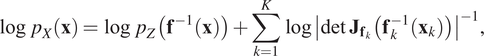(3)$$ \log \hskip0.3em {p}_X\left(\mathbf{x}\right)=\log \hskip0.3em {p}_Z\left({\mathbf{f}}^{-1}\left(\mathbf{x}\right)\right)+\sum \limits_{k=1}^K\log {\left|\det \hskip0.3em {\mathbf{J}}_{{\mathbf{f}}_k}\left({\mathbf{f}}_k^{-1}\left({\mathbf{x}}_k\right)\right)\right|}^{-1}, $$

where $ {\mathbf{x}}_k $ is an intermediate variable $ {\mathbf{x}}_k={\mathbf{f}}_k\left({\mathbf{x}}_{k-1}\right) $. In practice, the transformation is often set up as a trainable function $ {\mathbf{f}}_{\theta } $ with parameters $ \theta $. By using the CVF, the transformation $ {\mathbf{f}}_{\theta } $ can be trained via direct likelihood maximization, and for numerical reasons, the log form in Equation (3) is maximized in training:

(4)$$ \underset{\theta }{\max}\hskip1em \log \hskip0.3em {p}_X\left(\mathbf{x};\boldsymbol{\theta} \right)=\log \hskip0.3em {p}_Z\left({\mathbf{f}}_{\boldsymbol{\theta}}^{-1}\left(\mathbf{x}\right)\right)+\log {\left|\det \hskip0.3em {\mathbf{J}}_{{\mathbf{f}}_{\boldsymbol{\theta}}}\left({\mathbf{f}}_{\boldsymbol{\theta}}^{-1}\left(\mathbf{x}\right)\right)\right|}^{-1}. $$

Here, the likelihood $ {p}_X\left(\mathbf{x};\boldsymbol{\theta} \right) $ is parameterized by the trainable parameters $ \boldsymbol{\theta} $ of the transformation $ {\mathbf{f}}_{\boldsymbol{\theta}} $ and the historical samples of the target distribution x take the role of training data.

In the past 6 years, many flow construction methods have been proposed (e.g., Dinh et al., Reference Dinh, Krueger and Bengio2015, Reference Dinh, Sohl-Dickstein and Bengio2017). A prominent normalizing flow model is RealNVP (Dinh et al., Reference Dinh, Sohl-Dickstein and Bengio2017), which uses an affine coupling layer and has shown promising results in a prior application to time series data (Zhang and Zhang, Reference Zhang and Zhang2020). The idea of the RealNVP affine coupling layer is to split the full input vector $ \mathbf{z}={\mathbf{z}}_{1:D} $ of dimension D and apply an affine transformation to one part of the input vector $ {\mathbf{z}}_{d+1:D} $ conditioned on the remaining part of the input vector $ {\mathbf{z}}_{1:d} $ that is kept constant. Here, d is usually set to $ d=D/2 $ to allow for maximal interaction between dimensions but can take other values $ 1<d<D $, for example, if D is uneven. The standard forward transformation $ {\mathbf{f}}_{\mathrm{CL}}:\mathbf{z}\to \mathbf{x} $ is given by

(5)$$ {\mathbf{x}}_{1:d}={\mathbf{z}}_{1:d}, $$

(6)$$ {\mathbf{x}}_{d+1:D}=\exp \left({\mathbf{s}}_{\boldsymbol{\theta}}\left({\mathbf{z}}_{1:d}\right)\right)\hskip0.3em \odot \hskip0.3em {\mathbf{z}}_{d+1:D}+{\mathbf{t}}_{\boldsymbol{\theta}}\hskip0.3em \left({\mathbf{z}}_{1:d}\right), $$

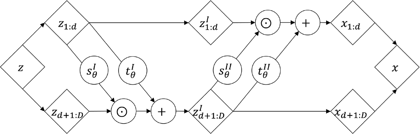
where the functions $ {\mathbf{s}}_{\boldsymbol{\theta}}\left({\mathbf{z}}_{1:d}\right) $ and $ {\mathbf{t}}_{\boldsymbol{\theta}}\left({\mathbf{z}}_{1:d}\right) $ are feed-forward ANNs called conditioner networks with parameters θ and input and output dimensions d and $ D-d $, respectively. The $ \odot $ operator denotes elementwise multiplication. Note that when applied as a composition in alternating form, RealNVP can build flexible and easily invertible transformations with tractable Jacobian determinants. A visual description of a composition of two affine coupling layers is presented in Figure 1.

Figure 1. Real non-volume preserving transformation (Dinh et al., Reference Dinh, Sohl-Dickstein and Bengio2017) with two coupling layers with alternating identity and affine transformations. Arrows point in generative direction. Compositions may include more than two coupling layers. Functions $ {\mathbf{s}}_{\boldsymbol{\theta}}^I\left({\mathbf{z}}_{1:d}\right) $, $ {\mathbf{t}}_{\boldsymbol{\theta}}^I\left({\mathbf{z}}_{1:d}\right), $ $ {\mathbf{s}}_{\boldsymbol{\theta}}^{II}\left({\mathbf{z}}_{d+1:D}^I\right) $, and $ {\mathbf{t}}_{\boldsymbol{\theta}}^{II}\left({\mathbf{z}}_{d+1:D}^I\right) $ are trainable artificial neural networks with parameters θ.

The affine coupling layer in Equations (5) and (6) has the advantage that the Jacobian of the transformation f_CL is a lower triangular matrix, that is,

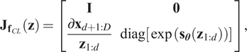(7)$$ {\mathbf{J}}_{{\mathbf{f}}_{CL}}\left(\mathbf{z}\right)=\left[\begin{array}{cc}\mathbf{I}& \mathbf{0}\\ {}\frac{\partial {\mathbf{x}}_{d+1:D}}{{\mathbf{z}}_{1:d}}& \operatorname{diag}\left[\exp \left({\mathbf{s}}_{\boldsymbol{\theta}}\left({\mathbf{z}}_{1:d}\right)\right)\right]\end{array}\right], $$

which means that the log of the absolute value of its determinant is simply given by

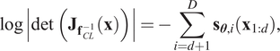
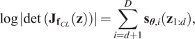(8)$$ \log \left|\det \hskip0.3em \left({\mathbf{J}}_{{\mathbf{f}}_{CL}}\left(\mathbf{z}\right)\right)\right|=\sum \limits_{i=d+1}^D{\mathbf{s}}_{\boldsymbol{\theta}, i}\left({\mathbf{z}}_{1:d}\right), $$

and the Jacobian of the inverse transformation $ {\mathbf{f}}_{CL}^{-1}:\mathbf{x}\to \mathbf{z} $ satisfies

(9)$$ \log \left|\det \hskip0.3em \left({\mathbf{J}}_{{\mathbf{f}}_{CL}^{-1}}\left(\mathbf{x}\right)\right)\right|=-\sum \limits_{i=d+1}^D{\mathbf{s}}_{\boldsymbol{\theta}, i}\left({\mathbf{x}}_{1:d}\right), $$

according to the inverse function theorem (Papamakarios et al., Reference Papamakarios2020). With Equations (8) and (9), the log-Jacobian determinant is computed from a simple evaluation of the forward or inverse transformation.

For a more detailed introduction and a review of other normalizing flow designs, the interested reader is referred to the original RealNVP paper by Dinh et al. (Reference Dinh, Sohl-Dickstein and Bengio2017) and the review articles by Kobyzev et al. (Reference Kobyzev, Prince and Brubaker2020) and Papamakarios et al. (Reference Papamakarios2020) .

3. Principal Component Density Estimation

In this section, we first discuss the effects of manifolds on the Jacobians and the contradiction between manifolds and diffeomorphic transformations and visualize how distributions get smeared out at the example of a one-dimensional distribution embedded in two-dimensional space. Second, we show how unlike many other dimensionality reduction techniques PCA can be used in combination with standard normalizing flows for manifold density estimation with tractable and direct likelihood computation.

3.1. Normalizing flows and manifolds

Normalizing flows are transformations between the space of observable variables (target distribution) and a latent space with independent variables, that is, a space with zero covariance (base distribution; Papamakarios et al., Reference Papamakarios2020). As a consequence, normalizing flows disentangle the information contained in the observable variables, for example, the power generation over a given period, to the set of independent latent variables, that is, the normalizing flow transformation eliminates the correlation between the dimensions (Kobyzev et al., Reference Kobyzev, Prince and Brubaker2020; Papamakarios et al., Reference Papamakarios2020). For the disentanglement to function properly, the normalizing flow transformation f and its inverse $ {\mathbf{f}}^{-1} $ must be continuously differentiable, that is, the Jacobian of f must be non-singular for $ {\mathbf{f}}^{-1} $ to be differentiable and vice versa (Papamakarios et al., Reference Papamakarios2020). The distributions of many datasets do not occupy the entire space of observable variables, that is, the distributions lie on lower-dimensional manifolds (Fefferman et al., Reference Fefferman, Mitter and Narayanan2016). A transformation from a latent space Gaussian with equal dimensionality to the space of observable variables must compress the Gaussian samples to the lower-dimensional space and, therefore, have a singular Jacobian (Hyvärinen and Pajunen, Reference Hyvärinen and Pajunen1999; Behrmann et al., Reference Behrmann, Vicol, Wang, Grosse, Jacobsen, Banerjee and Fukumizu2021). Consequently, a Gaussian with equal dimensionality cannot be matched to a manifold distribution using a diffeomorphic transformation.

However, normalizing flow transformations like RealNVP (Dinh et al., Reference Dinh, Sohl-Dickstein and Bengio2017) are designed to be diffeomorphic between spaces of equal dimensionality. When applied to manifold data, they have to include all latent space variables in the transformation with a nonzero gradient even if the data do not show any related variance. This leads to a contradiction between a problem that cannot be solved using a diffeomorphism and a strictly diffeomorphic normalizing flow. In practice, fitting a normalizing flow to manifolds leads to numerically singular Jacobians (Behrmann et al., Reference Behrmann, Vicol, Wang, Grosse, Jacobsen, Banerjee and Fukumizu2021) as the training attempts to compress the Gaussian to the lower-dimensional space. For sampling, the learned distribution is then smeared out around the true distribution (Brehmer and Cranmer, Reference Brehmer and Cranmer2020), causing skewed distribution densities and generation of out-of-distribution data.

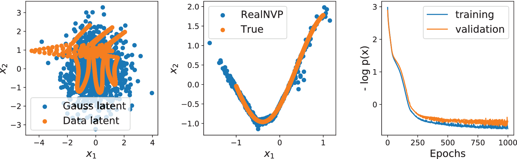
To illustrate this fundamental problem, we train two RealNVP models with identical architecture on samples of a one-dimensional, uniform distribution embedded in a two-dimensional curve and a two-dimensional distribution. Figures 2 and 3 show the encoded training data (Data latent) and samples of a two-dimensional Gaussian (Gauss latent) on the left, the training data (True) and samples generated using the RealNVP in the center, and training and validation loss on the right for the two different distributions, respectively. The example in Figure 2 highlights that the points from the one-dimensional curve remain on a one-dimensional curve after the transformation with the diffeomorphism. Accordingly, any point in the latent space outside of this curve has no counterpart in the true data distribution. Thus, the samples drawn in the Gaussian latent space (left) are transformed to out-of-distribution data, as can be seen by the RealNVP samples outside of the curve in the center of Figure 2. Nevertheless, the generated distributions resemble the shape of the true distributions, and the out-of-distribution samples may not be noticed for higher-dimensional distributions, for example, time series, that cannot be viewed in their ambient space.

Figure 2. Real non-volume preserving transformation (RealNVP; Dinh et al., Reference Dinh, Sohl-Dickstein and Bengio2017) trained on 1D manifold in 2D space (x ₁,x ₂). Left: samples of 2D Gaussian (blue) and training data after transformation to Gaussian (orange). Center: samples from trained RealNVP (blue) and true (orange) data distribution. Right: training and validation loss over number of epochs.

Figure 3. Real non-volume preserving transformation (RealNVP; Dinh et al., Reference Dinh, Sohl-Dickstein and Bengio2017) trained on 2D kite-shaped distribution in 2D space (x ₁,x ₂). Left: samples of 2D Gaussian (blue) and training data after transformation to Gaussian (orange). Center: samples from trained RealNVP (blue) and true (orange) data distribution. Right: training and validation loss over number of epochs.

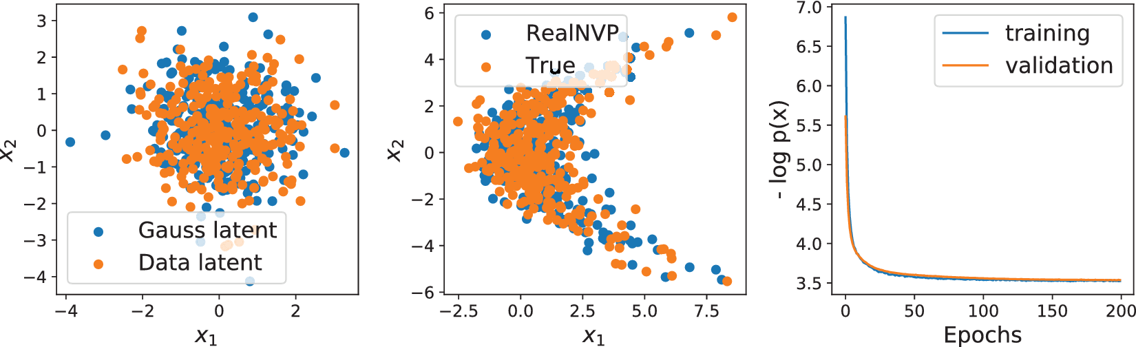
The absolute values of the loss functions are not comparable as they describe different distributions. However, while the validation loss of the one-dimensional example in Figure 2 indicates overfitting and unstable training, the validation loss of the two-dimensional example in Figure 3 indicates good generalization, stable training, and convergence in fewer epochs. Besides the loss functions, the data transformed to the latent space in the left of Figure 3 and the RealNVP generated data in the center of Figure 3 show good matches of the Gaussian and true data distribution, respectively.

3.2. Principal component flow layer

Given an available injective map $ \psi :{\mathrm{\mathbb{R}}}^M\to {\mathrm{\mathbb{R}}}^D,\mathbf{x}=\psi \left(\tilde{\mathbf{x}}\right) $ with $ D>M $ transforming data points from the lower-dimensional latent space $ \tilde{\mathbf{x}} $ to their full-space embedding x, a flow on a Riemannian manifold can be built (Gemici et al., Reference Gemici, Rezende and Mohamed2016). Since the injective map expands the dimensionality, the typical CVF relation (Equation (3)) of infinitesimal volumes using the Jacobian determinant does no longer apply. Instead, the relation between the two infinitesimal volumes is given by (Ben-Israel, Reference Ben-Israel2000)

(10)$$ dX=\sqrt{\det \left({\mathbf{J}}_{\psi}^T{\mathbf{J}}_{\psi}\right)} dZ, $$

with Jacobian $ {\mathbf{J}}_{\psi } $ of the mapping $ \psi $. The generalized form of the CVF for the injective flow then is (Ben-Israel, Reference Ben-Israel2000; Gemici et al., Reference Gemici, Rezende and Mohamed2016):

(11)$$ {p}_X(\mathbf{x})={p}_Z(\psi {(\mathbf{x})}^{-1}){[|\det ({\mathbf{J}}_{\psi }{({\psi}^{-1}(\mathbf{x}))}^T{\mathbf{J}}_{\psi }({\psi}^{-1}(\mathbf{x})))|]}^{-0.5} $$

For the injective map ψ to be applicable for the use in combination with normalizing flows, its inverse $ {\psi}^{-1} $ must be available and easy to compute, and the Jacobian determinant term in Equation (11) must be computationally tractable during training. Brehmer and Cranmer (Reference Brehmer and Cranmer2020) propose to build an injective map by fixing some of the latent space dimensions of a normalizing flow to a constant. However, their approach still results in expensive Jacobian computations and requires balancing a reconstruction loss with the likelihood maximization. To avoid expensive Jacobian computations and achieve easily invertible dimensionality reduction, we exploit the isometric, that is, distance preserving, characteristic of the affine PCA (Pearson, Reference Pearson1901). PCA is based on the singular value decomposition of the sample covariance matrix $ {\mathbf{K}}_{X,X} $ of the data distribution X, that is,

(12)$$ {\mathbf{K}}_{X,X}=\frac{1}{N-1}\sum \limits_{i=1}^N\left({\mathbf{x}}_i-{\boldsymbol{\mu}}_X\right){\left({\mathbf{x}}_i-{\boldsymbol{\mu}}_X\right)}^T=\mathbf{U}\mathtt{\varSigma }{\mathbf{V}}^{-1}, $$

where N is the number of data points, x are the data points, and μ_x is the empirical mean vector of the distribution. The covariance matrix $ {\mathbf{K}}_{X,X} $ is decomposed into a diagonal matrix of singular values $ \mathtt{\varSigma} $ and two unitary matrices U and V of left and right singular vectors, respectively. The columns of the matrix of right singular vectors V corresponding to the largest singular values are called the principal components of the data distribution X. By truncating the columns with small or zero singular values, we can use the resulting semi-orthogonal matrix V_P for the affine embedding function:

(13)$$ \mathbf{x}={\psi}_{\mathrm{PCA}}\left(\tilde{\mathbf{x}}\right)={\mathbf{V}}_P\tilde{\mathbf{x}}+{\boldsymbol{\mu}}_X $$

with V_P as the truncated matrix of right singular vectors and μ_x as the mean value of the distribution (Pearson, Reference Pearson1901).

In general, isometries are defined via:

(14)$$ {\mathbf{J}}_{\psi }{\left(\tilde{\mathbf{x}}\right)}^T{\mathbf{J}}_{\psi}\left(\tilde{\mathbf{x}}\right)={\mathbf{I}}_M,\hskip1em \forall \tilde{\mathbf{x}}\in {\mathrm{\mathbb{R}}}^M. $$

Here, I_M is the M × M identity matrix. For PCA, Equation (14) holds as the Jacobian of $ {\psi}_{\mathrm{PCA}} $ is $ {\mathbf{J}}_{\psi_{\mathrm{PCA}}}\left(\tilde{\mathbf{x}}\right)={\mathbf{V}}_P $, where V_P is semi-orthogonal. Thus:

(15)$$ {\mathbf{J}}_{\psi_{\mathrm{PCA}}}{\left(\tilde{\mathbf{x}}\right)}^T{\mathbf{J}}_{\psi_{\mathrm{PCA}}}\left(\tilde{\mathbf{x}}\right)={\mathbf{V}}_P^T{\mathbf{V}}_P={\mathbf{I}}_M,\hskip1em \forall \tilde{\mathbf{x}}\in {\mathrm{\mathbb{R}}}^M. $$

The isometric property of PCA results in two major advantages for the combination with normalizing flows. First, the PCA (pseudo-)inverse can be computed using the transpose of V_P:

(16)$$ \tilde{\mathbf{x}}={\psi}_{\mathrm{PCA}}^{-1}\left(\mathbf{x}\right)={\mathbf{V}}_P^T\left(\mathbf{x}-{\mu}_X\right), $$

which makes the inverse explicit and computationally efficient. Second, the PDF described by the CVF is invariant to the PCA dimensionality reduction, as the expression in Equation (15) enters in the Jacobian determinant term of Equation (11), that is,

(17)$$ {\left[\left|\det \left({\mathbf{J}}_{\psi_{\mathrm{PCA}}}{\left(\tilde{\mathbf{x}}\right)}^T{\mathbf{J}}_{\psi_{\mathrm{PCA}}}\left(\tilde{\mathbf{x}}\right)\right)\right|\right]}^{-0.5}={\left[\left|\det \left(\underset{={\mathbf{I}}_M}{\underbrace{{\mathbf{V}}_P^T{\mathbf{V}}_P}}\right)\right|\right]}^{-0.5}=1,\hskip1em \forall \tilde{\mathbf{x}}\in {\mathrm{\mathbb{R}}}^M. $$

When we build a composition of a standard normalizing flow and the PCA following Equation (3), it becomes apparent that the PCA transformation does not influence the PDF described by the CVF:

(18)$$ {\displaystyle \begin{array}{c}\log \hskip0.3em {p}_X\left(\mathbf{x}\right)=\log \hskip0.3em {p}_Z\left({\mathbf{f}}^{-1}\circ {\psi}_{\mathrm{PCA}}^{-1}\left(\mathbf{x}\right)\right)+\log \left|\det \hskip0.3em \left({\mathbf{J}}_{{\mathbf{f}}^{-1}}\left({\psi}_{\mathrm{PCA}}^{-1}\left(\mathbf{x}\right)\right)\right)\right|+\underset{=0}{\underbrace{\log {\left[\left|\det \hskip0.3em \left({\mathbf{V}}_P^T{\mathbf{V}}_P\right)\right|\right]}^{-0.5}}}\\ {}=\log \hskip0.3em {p}_Z\left({\mathbf{f}}^{-1}\left(\tilde{\mathbf{x}}\right)\right)+\log \left|\det \hskip0.3em \left({\mathbf{J}}_{{\mathbf{f}}^{-1}}\left(\tilde{\mathbf{x}}\right)\right)\right|.\end{array}} $$

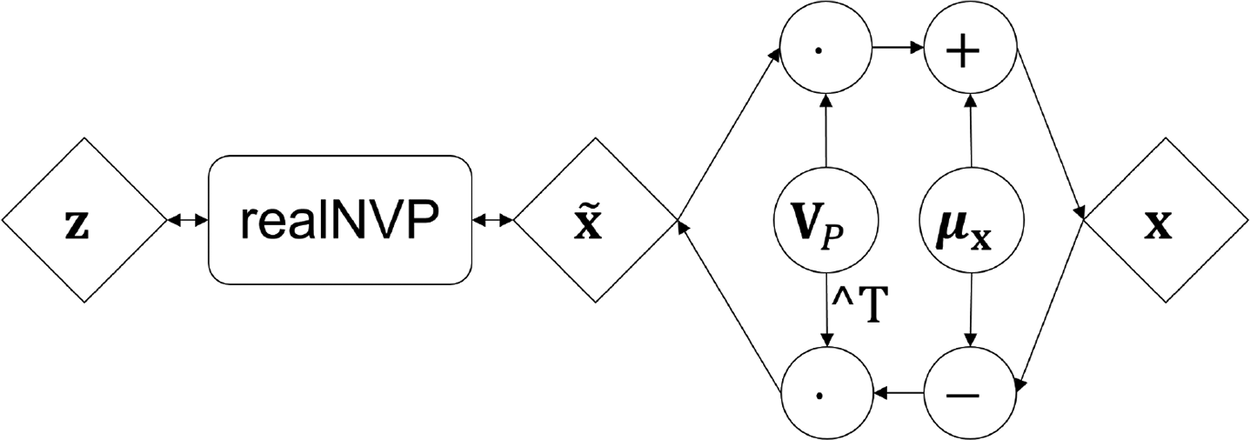
In Equation (18), $ \tilde{\mathbf{x}}={\psi}_{\mathrm{PCA}}^{-1}\left(\mathbf{x}\right) $ is the lower-dimensional representation (Equation (13)) and f is a standard normalizing flow model, for example, RealNVP (Dinh et al., Reference Dinh, Sohl-Dickstein and Bengio2017). Because PCA does not influence the CVF, it can be solved prior to fitting the normalizing flow and the PCF layer does not include trainable variables for the log-likelihood maximization. Hence, we avoid composite loss functions that balance reconstruction loss and likelihood maximization as in Brehmer and Cranmer (Reference Brehmer and Cranmer2020). The available inverse and separation of PCA fit and normalizing flow training make the use of PCA computationally very efficient, as neither the inverse nor the Jacobian has to be computed at any point. Note that the efficient inverse and the omittable Jacobian determinant do not transfer to most other dimensionality reduction techniques, for example, local linear embeddings (Roweis and Saul, Reference Roweis and Saul2000) or diffusion maps (Coifman and Lafon, Reference Coifman and Lafon2006). A graphical description of the combination of the PCA and RealNVP is shown in Figure 4.

Figure 4. Principal component flow structure with principal component analysis layer as last layer in generative direction and real non-volume preserving transformation (see Figure 1) as trainable normalizing flow in lower-dimensional space.

4. Numerical Experiments

In this section, we train the PCF on real-world time series data. The three different datasets considered contain data of PV power generation, wind power generation, and load demand, where each represents the total values in Germany in the years 2013–2015 (Open Power Systems Data, 2019). In the analysis below, we treat each of the time series independently. Prior to any processing, we clean the data of any days with missing values. To the best of our knowledge, there are no curtailment effects in the data. PV and wind scenarios are scaled by the installed capacity at each time step. Thus, the networks are trained on the so-called capacity factor. The load demand data are scaled to the [0,1] interval resulting in what we refer to as the demand factor in the following. Learning the capacity factor distribution avoids skewness of the distribution due to the addition of further generation capacity in the given time frame. We have not observed long-term trends in the load demand data of the selected period. To be processed by the normalizing flow, the univariate time series are cut into intervals of 1 day each. With sampling intervals of 15 min, this leads to a set of 96-dimensional time series fragments that will serve as training data, that is, a set of 96-dimensional vectors, which is a typical approach in the field of DGM scenario generation (Chen et al., Reference Chen, Wang, Kirschen and Zhang2018c; Zhang and Zhang, Reference Zhang and Zhang2020). This approach is known as multivariate prediction (Ziel and Weron, Reference Ziel and Weron2018) as multiple time steps are predicted at the same time.

For a comparison with more established scenario generation approaches, we also generate scenarios using Copulas and W-GANs. In contrast to autoregressive models (Sharma et al., Reference Sharma, Jain and Bhakar2013) and similar to normalizing flows, Copulas and W-GANs describe the full distribution independent of conditional inputs. We use the linear interpolation of the inverse cumulative distribution function to fit the Copula to the data (Pinson et al., Reference Pinson, Madsen, Nielsen, Papaefthymiou and Klöckl2009), and for the W-GANs, we follow the approach by Chen et al. (Reference Chen, Wang, Kirschen and Zhang2018c). Note that both Copulas and W-GANs use the same idea of multivariate scenario generation, that is, treating scenarios as a vector rather than a sequence of values.

First, we investigate the manifold dimensionality of the datasets by looking at the explained variance ratio of the principal components. The explained variance ratio is the value of the singular values of the covariance matrix scaled by their sum, that is, the relative amount of variance in the data, which is described by the right singular vector (the principal component) corresponding to the given singular value (Tipping and Bishop, Reference Tipping and Bishop1999). As an indicator of the manifold dimensionality, we look at the cumulative explained variance (CEV), which describes how much of the information in terms of variance is maintained when the data are compressed to the space of principal components. Table 1 lists some relevant CEV values and the corresponding latent space dimensionality for our datasets. The results show that a significantly reduced dimensionality maintains close to all of the variance information in the data. The 100% threshold is reached when the latent dimensionality is equal to the numerical rank of the covariance matrix. The PV data reach this threshold at a latent dimensionality of 62. Note that the 100% CEV appears with fewer principal components than dimensions of the data, if either one or more of the dimensions have zero variance or if there is an exact linear dependency of one of the dimensions on one or more of the other dimensions. Another important thing to consider is that the PCA is fitted using the empirical covariance matrix, that is, with a finite number of samples. Hence, the numerical rank might be different from the rank of the covariance matrix of the process and the low variance components identified by the PCA may not be fully representative of the underlying process. Hence, the low-variance and high-frequency components identified by the PCA may not be desired.

Table 1. Number of principal components for cumulative explained variance (CEV). Data with 15-min resolution (96 dimensions) from Open Power Systems Data (2019).

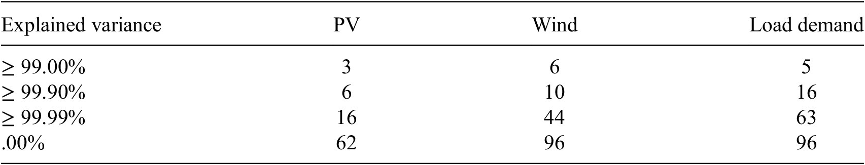
Abbreviation: PV, photovoltaics.

We train FSNF and PCF models on each of the three different datasets and compare the generated to the historical data (target). For each dataset, we select two latent dimensionalities, namely, 16 and 62 for PV to represent 99.99 and 100% of the variance, and 6 and 10 for wind as well as 5 and 16 for demand to represent 99 and 99.9% of the variance, respectively. In each training, 20% of the 1,096 scenarios are set aside as validation sets for hyperparameter tuning and to avoid overfitting. All of the following analysis is performed using the full historical scenario sets in comparison to sets of generated scenarios, to avoid random errors in the evaluation as a result of too few data points.

We find that, for all networks, five RealNVP affine coupling layers with fully connected conditioner networks with two hidden layers of the same size as the input dimension each are sufficient and additional complexity does not improve the representation. All normalizing flow models are implemented using the Python-based machine learning libraries TensorFlow version 2.4.0 (Abadi and Agarwal, Reference Abadi and Agarwal2015) and TensorFlow-Probability version 0.12.1 (Dillon et al., Reference Dillon, Langmore, Tran, Brevdo, Vasudevan, Moore, Patton, Alemi, Hoffman and Saurous2017). We use the PCA routine from the open-source scikit-learn Python library version 0.24.0 (Pedregosa et al., Reference Pedregosa, Varoquaux, Gramfort, Michel, Thirion, Grisel, Blondel, Prettenhofer, Weiss, Dubourg, Vanderplas, Passos, Cournapeau, Brucher, Perrot and Duchesnay2011) for dimensionality reduction.

We estimate the PDF of the data using kernel density estimation (KDE) with Gaussian kernels (Parzen, Reference Parzen1962) as shown in Figure 5. The top line of Figure 5 shows the PDF plots of the historical scenarios, FSNF-generated scenarios, and scenarios generated using the proposed PCF for each of the three datasets. For reference, Figure 5 compares the Copula- and W-GAN-generated scenario PDFs with the historical scenarios, in the second line.

Figure 5. Comparison of the probability density function from kernel density estimation (Parzen, Reference Parzen1962). Top: historical data (target, solid lines), generated data from full-space normalizing flow (dashed lines), and generated data from principal component flow (dotted lines and dash-dotted lines). Bottom: historical data (target, solid lines), generated data from the Copula (dotted lines), and generated data from Wasserstein generative adversarial network (dash-dotted lines). Left: photovoltaic capacity factor. Center: wind capacity factor. Right: demand factor.

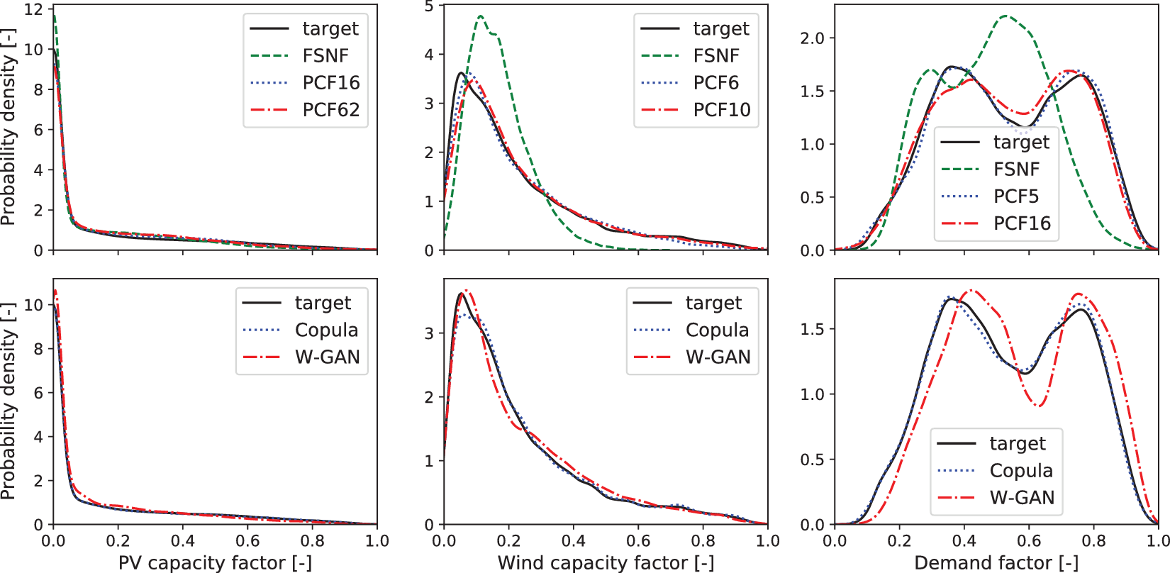
For the PV data in the left of Figure 5, the data from all three normalizing flow structures appear to match the distribution. The FSNF data exhibit a higher density than the target for capacity factors smaller than 0.05, between 0.1 and 0.45, and a lower density above a certain capacity factor of 0.45. The PCF62 data show an overestimation between capacity factors of 0.1 and 0.4; however, the PCF62 density is closer to the density of the target distribution than the FSNF density, in particular, for capacity factors below 0.1. Finally, the PCF16 data distribution is closest to the target distribution with good fits for capacity factors smaller than 0.2 and similar deviations from the target as observed with the FSNF and the PCF62.

For the wind capacity factor (center of Figure 5) and the demand factor (right of Figure 5), we observe a more drastic overestimation of the PDF for the highest densities and an underestimation of the tails by the FSNF. As for the PV scenarios, the density estimates for wind and load demand scenarios show an improved approximation of the distribution through dimensionality reduction with PCA, although the covariance matrices are not rank deficient. It appears that the FSNF tends to ignore rare events during the likelihood maximization and thus overestimates the areas of high density. With a lower dimensionality, rare events occupy a relatively larger space and are therefore more likely to be considered by the PCF likelihood maximization. Furthermore, the PDF fits of both wind and demand appear to improve by considering fewer principal components. By adding more principal components to get from 99 to 99.9% CEV, the training problem becomes less well conditioned as the additional dimensions are only narrowly occupied by data, that is, the distribution comes closer to a lower-dimensional manifold.

The bottom line of Figure 5 shows good matches of PV and wind capacity factor PDFs for both Copulas and W-GANs. The Copula scenarios also show a matching demand factor PDF, while the W-GAN results in a skewed PDF. A comparison of the top and bottom lines of Figure 5 highlights that PDF representations by the PCF are as good or better compared to the literature approaches.

Note that an exact evaluation of the KDE plot can be misleading since the KDE results are not exact, in particular, at the tails of the distribution and in low-density parts (Wied and Weißbach, Reference Wied and Weißbach2012). However, the trends for all three datasets show improved fits of the PCF setups compared to the FSNF, which indicates better distribution fits due to the dimensionality reduction.

To support the results from the visual comparison of KDE plots, we run a Kolmogorov–Smirnov test (KS-test; Hodges, Reference Hodges1958). The KS-test is used to judge whether two distinct sets of samples stem from the same distribution. Table 2 lists the p-values (p-value $ \in \left[0,1\right]\Big) $ of the tests. In general, high p-values (≥.1) can be interpreted as a match of distributions, and low p-values indicate that the two sample sets stem from different distributions (Hodges, Reference Hodges1958). For all three datasets, the p-values of the FSNF indicate that the historical and the generated data do not follow the same distribution. In contrast, the p-values for PCF16 for PV, PCF6 for wind, and PCF5 for load demand are ≥.1, indicating a good representation of the historical data distribution. The PCF10 for wind and the PCF16 for demand show p-values of ≥.05 and ≥.01, which still indicate good matches of the distribution and significantly better matches compared to the FSNF. The PCF62 for PV gives a lower p-value and hence lower confidence that the data stem from the historical data distribution. This result matches the observations in Figure 5, where we observed a slightly worse fit from PCF62 compared to PCF16. Still, there is a significant improvement compared to the FSNF. Furthermore, the KS-test confirms our observation of increasing quality of fit for the 99% CEV compared to the 99.9% CEV.

Table 2. p-Values (p-value $ \in \left[0,1\right] $) of Kolmogorov–Smirnov test (Hodges, Reference Hodges1958): statistical comparison of historical and generated data. High p-values (≥.1) indicate high probability that generated scenarios have same distribution as the historical scenarios. Results indicating a good match of the distributions are marked with an asterisk *.

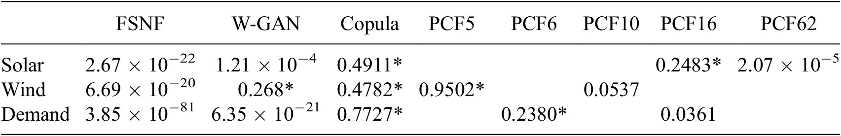
Abbreviations: FSNF, full space normalizing flow; PCF, principal component flow, W-GAN, Wasserstein generative adversarial network.

The KS-test of the reference models returns high p-values for all datasets for the Copula-generated scenarios, while only the wind capacity factor shows a high p-value among the W-GAN-generated scenarios. In general, the KS-test indicates good matching distributions only for Copulas and for the PCFs with low numbers of principal components.

In conclusion, the PCF returns significantly better fits of the distribution compared to the FSNF. Furthermore, the PDF fits by the PCF are at least as good or better compared to the literature methods. Considering fewer principal components appears to enhance the learning of the distributions, and accepting CEV values around 99% does not compromise the overall match of the distribution.

We use the power spectral density (PSD) based on the Welch transform (Welch, Reference Welch1967) to investigate in the frequency domain whether the FSNF and the PCF can reproduce the fluctuational behavior of the original time series. Figure 6 shows the PSD of the target distribution, the FSNF, and the PCF generated scenarios for the three considered datasets, respectively.

Figure 6. Power spectral density with Welch transform (Welch, Reference Welch1967). Top: historical data (target, solid lines), generated data from full-space normalizing flow (dashed lines), and generated data from PCF (dotted lines and dash-dotted lines). Bottom: historical data (target, solid lines), generated data from the Copula (dotted lines), and generated data from Wasserstein generative adversarial network (dash-dotted lines). Left: photovoltaic capacity factor. Center: wind capacity factor. Right: demand factor.

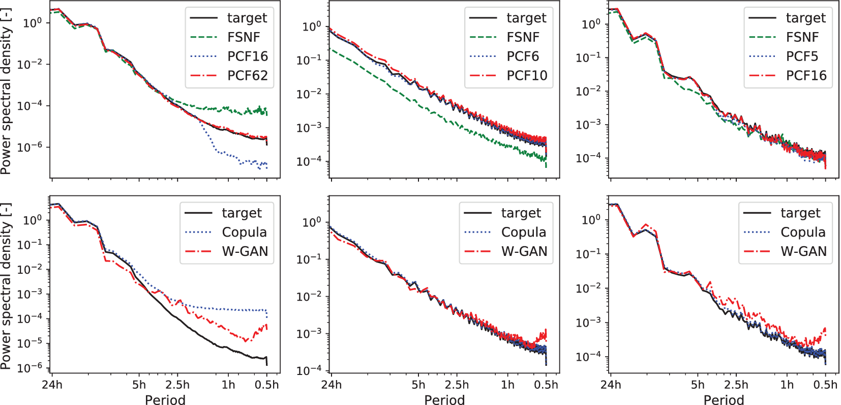
For the PV data, the target distribution shows high amplitudes (>10⁻⁴) for low frequencies up to $ \frac{1}{3.5\hskip0.1em h} $, which are well matched by all three DGMs. For higher frequencies ($ >\frac{1}{3.5\hskip0.1em h} $), the target amplitude declines faster than the FSNF amplitudes, indicating the generation of noisy behavior over shorter periods by the FSNF. In contrast, PCF16 produces lower amplitudes than the target distribution in the regime of frequencies $ >\frac{1}{2\hskip0.1em h} $, which indicates the filtering of some of the low amplitude fluctuation in the historical dataset. The PCF62 shows a good fit for the true behavior of the target up to the highest frequencies.

The PSD analysis for the wind data shows a good match of the frequency behavior for the data generated from the PCF6 and PCF10. The FSNF generated scenarios show a general underestimation of the amplitudes. Note that the wind data exhibit higher fluctuation on all frequencies compared to the PV data. Therefore, the fluctuations at high frequencies are represented in the principal components, and no filter effect can be observed. As the overall PSD shape is matched, the FSNF appears to find the right fluctuation behavior only with consistently lower amplitudes. Here, the narrower distribution described by the FSNF (see Figure 5) leads to a smaller range of scenarios and, therefore, lower amplitudes.

As for the wind scenarios, the PSD analysis of the load demand data in Figure 6 shows a good match of the PCF-generated scenarios to the historical data. The FSNF matches the overall PSD, but there are lower amplitudes between frequencies of $ >\frac{1}{8\hskip0.1em h} $ and $ >\frac{1}{2\hskip0.1em h} $.

The PSDs of the W-GAN-generated scenarios show an increase in amplitude for frequencies between $ \frac{1}{1\hskip0.1em h} $ and $ \frac{1}{0.5\hskip0.1em h} $ for all three datasets, indicating noisy scenarios. Furthermore, the PSDs of the PV capacity factor and the demand factor of the W-GAN-generated scenarios are higher compared to the historical scenario PSDs, that is, the W-GANs generate scenarios with unrealistically high fluctuations. The Copula-generated scenarios reproduce the PSDs of the wind capacity factor and the demand factor well. However, the Copula-generated PV capacity factor scenarios show high amplitudes for frequencies $ >\frac{1}{5\hskip0.1em h} $.

In conclusion, the PSD analysis of the PCF-generated scenarios clearly shows improved results for all datasets due to the dimensionality reduction compared to the FSNF. Some effects are specific to the PCA dimensionality reduction of the given data, for example, the filter effect observed for the PV data and the noise in the case of the load demand data. Among all considered scenario generation approaches, the PCF is the only approach that does not result in noisy behavior or otherwise higher fluctuations for all three datasets.

Finally, we investigate whether the PCF recovers the dimensions with zero variance that occur during the nighttime hours of the PV scenarios. Figure 7 shows the time between midnight and 4 am of five randomly selected scenarios from the historical data, the normalizing flow models, and Copula- and W-GAN-generated scenarios. The FSNF-generated scenarios clearly show noisy behavior. On the other hand, PCF16 and PCF62 do not show any noise and thus preserve the zero-variance feature of the respective dimensions. The W-GAN scenarios show high fluctuations without any structure, whereas the Copula scenarios appear to identify the zero variance of the nighttime hours correctly.

Figure 7. Five photovoltaic (PV) capacity factor scenarios from target, FSNF, PCF16, PCF62, Copula, and W-GAN, respectively. Time frame between midnight and 4 am. Abbreviations: FSNF, full-space normalizing flow; PCF, principal component flow; W-GAN, Wasserstein generative adversarial network.

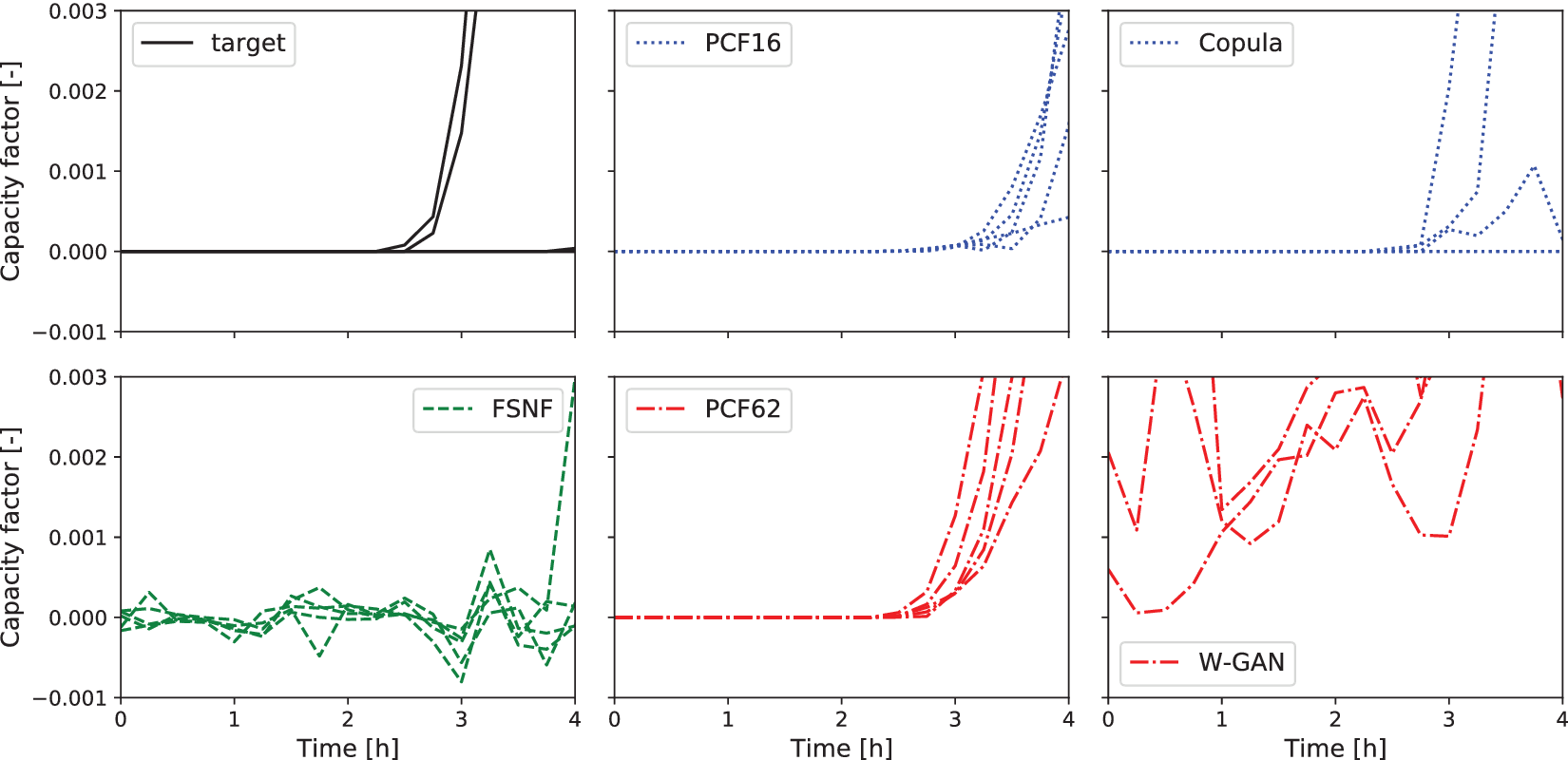
In addition to Figure 7, Table 3 lists the mean and the variance for the time steps between midnight and 4 am. The mean and variance values for PCF16 and PCF62 confirm the observations from Figure 7. Figure 7 and Table 3 highlight the “smeared-out” characteristic of the learned distribution as described in Section 3.1 and by Brehmer and Cranmer (Reference Brehmer and Cranmer2020). The results show that the FSNF is unable to detect dimensions of zero variance and does not accurately fit the manifold distribution, whereas PCF detects the manifold and correctly reproduces its features. In contrast to Figure 7, the mean and variance values of the Copula-generated scenarios highlight that the Copula does not identify the zero-variance characteristic of the nighttime hours. It appears that the Copula reproduces the zero-variance characteristic for most but not all of the scenarios.

Table 3. Marginal mean and variance values for photovoltaic scenarios between midnight and 4 am. Historical scenarios in comparison to FSNF-, PCF16-, and PCF62-generated scenarios as well as Copula- and W-GAN generated scenarios.

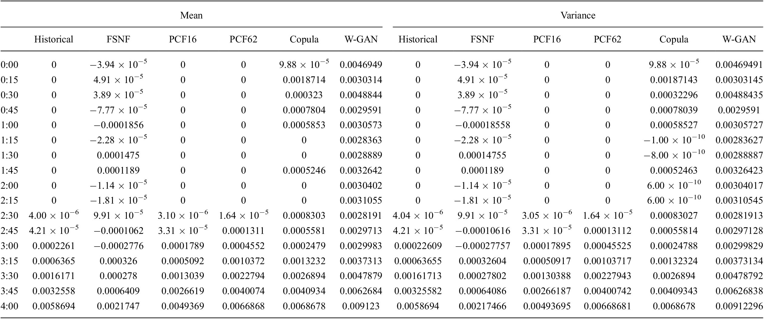
Abbreviations: FSNF, full-space normalizing flow; GAN, generative adversarial network; PCF, principal component flow.

In conclusion, the PCF is the only method among the considered approaches that consistently identifies the zero-variance characteristic of the PV scenarios during nighttime.

Nomenclature

Acronyms

ANN

artificial neural network

CEV

cumulative explained variance

CVF

change of variables formula

DGM

deep generative model

FSNF

full-space normalizing flow

GAN

generative adversarial network

KDE

kernel density estimation

NICE

nonlinear independent component estimation

PCA

principal component analysis

PCF

principal component flow

PDF

probability density function

PSD

power spectral density

PV

photovoltaic

RealNVP

real non-volume preserving transformation

VAE

variational autoencoder

Greek letters

θ

trainable parameters of conditioner networks $ {s}_{\theta } $ and $ {t}_{\theta } $

μ_X

mean value of distribution X

ψ

injective transformation

Latin letters

d

dimension

D

dimensionality of target distribution

f

transformation

f_CL

coupling layer transformation

I

identity matrix

J

Jacobian

K

number of transformations in composition

M

dimensionality <D

p_X/p_Y

probability density of X and Y

S_θ

conditioner network

t_θ

conditioner network

V

matrix of right singular vectors

V_P

truncated matrix of right singular vectors

x

target distribution sample

$ \tilde{\mathbf{x}} $

compressed target distribution sample

X

target distribution

z

base distribution sample

Z

base distribution