


Impact Statement
Deep Reinforcement Learning (DRL) algorithms, applied in Computational Fluid Dynamics (CFD), often face challenges due to high computational costs. In CFD, the expense of sample collection, from which DRL algorithms learn, can be significant. Effective DRL algorithm selection should aim at minimizing sample requirements while ensuring each training yields a usable solution. This paper evaluates three algorithms that utilize a replay buffer to store samples, potentially reducing sample needs and computational expenses. Notably, the SAC algorithm demonstrates consistent reliability and sample efficiency across diverse conditions, making it a promising choice for CFD applications and new case set-ups. Additionally, we introduce an aerodynamics benchmark, with increasing levels of data collection complexity, offering a valuable resource for future research in this field.
1. Introduction
Deep reinforcement learning (DRL) holds great promise for addressing optimization and control problems. It combines the capabilities of reinforcement learning (RL) approaches to control dynamic systems (Sutton and Barto, Reference Sutton and Barto2018), with the power of artificial neural networks to approximate functions (Goodfellow et al., Reference Goodfellow, Bengio and Courville2016), and has led to significant achievements in recent years. From board games (Silver et al., Reference Silver, Huang, Maddison, Guez, Sifre, van den Driessche, Schrittwieser, Antonoglou, Panneershelvam, Lanctot, Dieleman, Grewe, Nham, Kalchbrenner, Sutskever, Lillicrap, Leach, Kavukcuoglu, Graepel and Hassabis2016) to robotics (Ibarz et al., Reference Ibarz, Tan, Finn, Kalakrishnan, Pastor and Levine2021), or physics (Bellemare et al., Reference Bellemare, Candido, Castro, Gong, Machado, Moitra, Ponda and Wang2020; Degrave et al., Reference Degrave, Felici, Buchli, Neunert, Tracey, Carpanese, Ewalds, Hafner, Abdolmaleki, Casas, Donner, Fritz, Galperti, Huber, Keeling, Tsimpoukelli, Kay, Merle, Moret, Noury, Pesamosca, Pfau, Sauter, Sommariva, Coda, Duval, Fasoli, Kohli, Kavukcuoglu, Hassabis and Riedmiller2022), many domains have found new control solutions with the aid of DRL algorithms.
In the field of fluid mechanics, various problems have recently been addressed with this technique. Among them is the control of swimming fish with various objectives such as decreasing energy consumption (Novati et al., Reference Novati, Verma, Alexeev, Rossinelli, van Rees and Koumoutsakos2017; Verma et al., Reference Verma, Novati and Koumoutsakos2018) or pursuit-evasion (Borra et al., Reference Borra, Biferale, Cencini and Celani2022). Magnetic microswimmers were also successfully controlled through a uniform magnetic field (Amoudruz and Koumoutsakos, Reference Amoudruz and Koumoutsakos2022). Some studies focused on cylinder drag reduction, either through simulations at low Reynolds numbers (Rabault et al., Reference Rabault, Kuchta, Jensen, Reglade and Cerardi2019), in weakly turbulent conditions (Ren et al., Reference Ren, Rabault and Tang2021), or with an experimental approach (Fan et al., Reference Fan, Yang, Wang, Triantafyllou and Karniadakis2020). Other applications showed the capability of DRL for controlled gliding (Novati et al., Reference Novati, Mahadevan and Koumoutsakos2019), addressing Zermelo’s problem (Biferale et al., Reference Biferale, Bonaccorso, Buzzicotti, Clark Di Leoni and Gustavsson2019), navigating in vortical flow fields (Gunnarson et al., Reference Gunnarson, Mandralis, Novati, Koumoutsakos and Dabiri2021), and controlling chaotic problems such as the one-dimensional Kuramoto–Sivashinski equation (Bucci et al., Reference Bucci, Semeraro, Allauzen, Wisniewski, Cordier and Mathelin2019), or unsteady falling liquid films (Belus et al., Reference Belus, Rabault, Viquerat, Che, Hachem and Reglade2019). Modeling for large eddy simulation was also addressed with RL approaches: Novati et al. (Reference Novati, de Laroussilhe and Koumoutsakos2021) demonstrated the possibility of producing subgrid scale modeling in homogeneous turbulent flow, Kim et al. (Reference Kim, Kim, Kim and Lee2022) performed the same exercise for wall-bounded flows, and wall modeling was addressed in Bae and Koumoutsakos (Reference Bae and Koumoutsakos2022). This list is not comprehensive, and the number of DRL applications for fluid mechanics is growing fast. A recent review on the topic was proposed by Viquerat et al. (Reference Viquerat, Meliga, Larcher and Hachem2022).
The versatility of DRL comes at a price. Deep learning and reinforcement learning are based on well-established mathematical foundations, but their application to real-world problems often involves a lot of tricks and fine-tuning of hyperparameters. These practices rarely follow universal rules or even logical considerations at first glance and require countless hours of trial, debugging, and computing. Moreover, these methods are relatively new and their capabilities and limitations for dealing with real-world problems, such as those encountered in fluid mechanics, are still under investigation. Faced with a given system to control, one has to choose and tune the control problem formulation, as well as the algorithm, among multiple possibilities and with very few guidelines designed for the specific system at hand.
Researchers in the fluid mechanics community began to investigate some of the possibilities, analyze specific components, or propose significant improvements. For example, Belus et al. (Reference Belus, Rabault, Viquerat, Che, Hachem and Reglade2019) exploited the problem invariants and compared different solutions to deal with multiple actuators of the environment. Zeng and Graham (Reference Zeng and Graham2021) moved their problem to a reduced space by considering the flow symmetry. An other example is the work of Gunnarson et al. (Reference Gunnarson, Mandralis, Novati, Koumoutsakos and Dabiri2021) who explored the influence of the input data provided to the RL algorithm to observe the state of the environment, and compared these with optimal control, aware of the full flow field. Other studies of input data optimized the sensor layout feeding the algorithm (Paris et al., Reference Paris, Beneddine and Dandois2021; Xu and Zhang, Reference Xu and Zhang2023), or, in an experimental context, performed high-frequency filtering of the state to enable the agent to learn a successful policy (Fan et al., Reference Fan, Yang, Wang, Triantafyllou and Karniadakis2020). Another element of tremendous importance is the feedback signal provided to the RL algorithm indicating how well it performed. On this topic, Li and Zhang (Reference Li and Zhang2022) proposed adding stability information to the feedback signal, while Qin et al. (Reference Qin, Wang and Sun2021) implemented a reward function based on dynamic mode decomposition of the flow. Finally, some authors investigated the use of specific types of neural networks (Verma et al., Reference Verma, Novati and Koumoutsakos2018; Novati et al., Reference Novati, Mahadevan and Koumoutsakos2019) in the learning process. At the time of writing this article, very few comparisons between DRL algorithms can be found in the literature in the context of fluid mechanics. However, we can quote the study of Novati et al. (Reference Novati, Mahadevan and Koumoutsakos2019) that compared three different RL algorithms, namely, RACER, NAF, and PPO for controlled gliding, as well as three different studies (Biferale et al., Reference Biferale, Bonaccorso, Buzzicotti, Clark Di Leoni and Gustavsson2019; Castellanos et al., Reference Castellanos, Maceda, de la Fuente, Noack, Ianiro and Discetti2022; Pino et al., Reference Pino, Schena, Rabault and Mendez2023) that compared RL methods with other classic or more advanced control techniques while solving fluid mechanics problems.
Solving a given task with an RL algorithm relies on the collection of samples from an environment. When this environment is modelized with a computational fluid dynamics (CFD) solver, samples can be computationally expensive to collect,Footnote 1 which may hinder the applicability of DRL methods altogether. Therefore, the choice of the algorithm is mainly constrained by the high computing cost of experience collection: we want DRL algorithms that minimize the number of samples required to learn and for which each training run generates a usable policy, or, in other terms, algorithms that are both sample efficient and reliable. In addition, it calls for the creation of well-documented benchmarks of increasing complexity in terms of data collection cost. These are the two main objectives of this paper: (a) evaluate the sample efficiency, hyper-parameter sensitivity, and off-the-shelf reliability of existing DRL algorithms, and (b) establish a benchmark that can be solved at various costs, from a cheap low-order model to a costly CFD one. In contrast, the present work does not claim DRL policies to be superior to those obtained through more traditional methods, nor does it aim at a performance comparison, but rather tries to provide practical feedback and thoroughly evaluated guidelines for the implementation and practice of RL algorithms for fluid mechanics.
Regarding the first objective, DRL algorithms are numerous. In the context of fluid mechanics, the proximal policy optimization (PPO) algorithm (Schulman et al., Reference Schulman, Wolski, Dhariwal, Radford and Klimov2017) is often used (Viquerat et al., Reference Viquerat, Meliga, Larcher and Hachem2022). This algorithm, derived from the policy gradient theorem (Sutton et al., Reference Sutton, McAllester, Singh and Mansour1999), implements an on-policy optimization approach that prevents samples collected from the environment to be reused afterward in the learning process. This non-reusability is a heavy price to pay in situations where obtaining data is costly. Some researchers applying DRL techniques to fluid mechanics control problems choose algorithms from the family of approximate dynamic programming (Bertsekas, Reference Bertsekas2012) such as the twin delayed DDPG (TD3) algorithm (Fujimoto et al., Reference Fujimoto, Hoof and Meger2018; Fan et al., Reference Fan, Yang, Wang, Triantafyllou and Karniadakis2020) or its predecessor, the deep deterministic policy gradient (DDPG) algorithm (Lillicrap et al., Reference Lillicrap, Hunt, Pritzel, Heess, Erez, Tassa, Silver and Wierstra2016; Bucci et al., Reference Bucci, Semeraro, Allauzen, Wisniewski, Cordier and Mathelin2019; Kim et al., Reference Kim, Kim, Kim and Lee2022; Pino et al., Reference Pino, Schena, Rabault and Mendez2023). These algorithms are capable of sample reuse through the use of a replay buffer where experience samples are stored. The learning process therefore draws from the replay buffer. While TD3 is supposedly more reliable than DDPG, both exhibit some learning stability issues. As a result, they require fine-tuning of hyperparameters, which is highly time-consuming. In the same family of approximate dynamic programming, there is the state-of-the-art Soft Actor-Critic (SAC) algorithm (Haarnoja et al., Reference Haarnoja, Zhou, Abbeel and Levine2018). SAC introduces an additional entropy regularization term, which makes the optimization process more reliable and induces at the same time an adequate exploration of the environment, which can be critical for some applications. These three algorithms are studied in this paper. Note that other algorithms are used in the fluid mechanics community (see the review by Viquerat et al., Reference Viquerat, Meliga, Larcher and Hachem2022).
The algorithms benchmarked in this study all store samples in a replay buffer. With such algorithms, samples can be used several times in the learning process, which may decrease the number of samples required to produce a good policy. The use of a replay buffer also opens the field of possibilities regarding sample collection and usage. For example, among the samples stored in the replay buffer, those retained for learning can be chosen based on how much the agent will actually learn from them (Schaul et al., Reference Schaul, Quan, Antonoglou and Silver2016; Lahire et al., Reference Lahire, Geist and Rachelson2022). Besides, while classically filled with previous experiences obtained from interactions between the learning agent and the environment, the replay buffer may also be prefilled with data obtained elsewhere. Such data could come from a similar environment explored manually, from some experiments, or from some low-cost, low-order physics model. Reuse of previously or otherwise collected experience samples raises fundamental issuesFootnote 2 that would need to be addressed theoretically, but experience replay algorithms provide a potential modular way to transfer useful information collected in various ways and, therefore, to decrease the computational costs associated with sample collection. This is why such algorithms are evaluated in this paper. DDPG, TD3, and SAC are benchmarked against a fluid mechanics control problem and compared regarding reliability and sample efficiency, as well as the policies that they produce across a range of training configurations. Note that this study does not aim at designing a new state-of-the-art method, fine-tuning an existing method to achieve the best possible performance on a specific benchmark, or again outperforming existing baselines. Conversely, it takes a practitioner’s perspective and endeavors to assess the broad reliability and practical usability of some existing DRL algorithms in the fluid dynamics context.
As a second objective, we propose a benchmark case that can be approached with both (a) a low-fidelity approach that needs less than an hour on a computing core to train, and (b) a high-fidelity approach that solves the Navier–Stokes equations and is 1,200 times more expensive. The low computational cost of the former allows testing various algorithms and parameters. These are then used to setup the high-fidelity case, which is closer to a realistic context of application for fluid mechanics. The task consists in controlling an airfoil from an initial point A to reach a target point B. In the first task, the target B is kept in a fixed position during both the learning and testing of the policy (Figure 7), whereas in the second task, B may be anywhere in a given domain (Figure 16). The first task is a “learn by heart” problem while the second aims at learning a controller able to reach any point in a given domain and requires a closed-loop controller. The three DRL algorithms are evaluated on both tasks, when solving the physics with either a low-order or a high-fidelity model, and with various DRL hyperparameters, reward formulations, and environment parameters controlling the dynamics.
The paper is organized as follows: First, the benchmark problem is described as well as the two physics models, in Section 2. Then, Section 3 presents the control problem definition and some generalities about the RL algorithms benchmarked in the study. Section 4 and Section 5 are dedicated to the results of the first and second tasks, respectively.
2. Problem Description and Numerical Setup
An airfoil trajectory control problem is selected as a benchmark case: an airfoil (P) is initially placed at point A, and the controller optimizes the airfoil pitch rate $ \dot{\beta} $
, along its trajectory, in order to reach a target point B, as illustrated in Figure 1. There is no propulsion system in this problem: the airfoil is released with an initial velocity, and the controller has to learn how to glide towards B by controlling the airfoil pitch rate only. Two different tasks are considered. In the first task, A and B are kept in fixed positions (Figure 7), while in the second task, B may take any position in a given domain (Figure 16).
$ \dot{\beta} $
, along its trajectory, in order to reach a target point B, as illustrated in Figure 1. There is no propulsion system in this problem: the airfoil is released with an initial velocity, and the controller has to learn how to glide towards B by controlling the airfoil pitch rate only. Two different tasks are considered. In the first task, A and B are kept in fixed positions (Figure 7), while in the second task, B may take any position in a given domain (Figure 16).

Figure 1. Illustration of the airfoil trajectory control problem.
The problem considered is two-dimensional. The airfoil is a flat plate whose chord length is $ c=0.01\mathrm{m} $
, and whose thickness is 2% of the chord length. The fluid and flat plate densities are, respectively, equal to
$ c=0.01\mathrm{m} $
, and whose thickness is 2% of the chord length. The fluid and flat plate densities are, respectively, equal to $ {d}_f=1\mathrm{kg}\;{\mathrm{m}}^{-3} $
and
$ {d}_f=1\mathrm{kg}\;{\mathrm{m}}^{-3} $
and $ {d}_s=30\times {d}_f $
. The flat plate is released from a fixed initial position A = (
$ {d}_s=30\times {d}_f $
. The flat plate is released from a fixed initial position A = ( $ {x}_A=0 $
,
$ {x}_A=0 $
, $ {y}_A=0 $
), with an initial velocity purely horizontal and directed to the left:
$ {y}_A=0 $
), with an initial velocity purely horizontal and directed to the left: $ \overrightarrow{U_0}=-10\overrightarrow{x}\mathrm{m}\;{\mathrm{s}}^{-1} $
. After the release, the airfoil is only subject to aerodynamic forces and gravity. Based on the flat plate chord length, the initial velocity, and a kinematic viscosity
$ \overrightarrow{U_0}=-10\overrightarrow{x}\mathrm{m}\;{\mathrm{s}}^{-1} $
. After the release, the airfoil is only subject to aerodynamic forces and gravity. Based on the flat plate chord length, the initial velocity, and a kinematic viscosity $ \nu =3.333\times {10}^{-4}{\mathrm{m}}^2\;{\mathrm{s}}^{-1} $
, the Reynolds number is equal to
$ \nu =3.333\times {10}^{-4}{\mathrm{m}}^2\;{\mathrm{s}}^{-1} $
, the Reynolds number is equal to $ \mathit{\operatorname{Re}}=300 $
and remains almost constant along the trajectory. Note that in the remainder of the manuscript, “airfoil” and “flat plate” are used interchangeably.
$ \mathit{\operatorname{Re}}=300 $
and remains almost constant along the trajectory. Note that in the remainder of the manuscript, “airfoil” and “flat plate” are used interchangeably.
Such an aerodynamic control problem can be modeled through equations of various complexity, ranging from the Navier–Stokes equations to a simple analytical model. The present study uses two different levels of fidelity: the physics is either described through the unsteady Navier–Stokes equations (Section 2.1), or through a quasi-steady empirical model (Section 2.2). Both models are described in the following sections.
2.1. High-fidelity model based on the unsteady Navier–Stokes equations
The simulation of the fluid–solid interaction between the airfoil and the surrounding flow is performed with STAR-CCM+. The numerical approach is similar to the one used in Jardin and Doué (Reference Jardin and Doué2019). The evolution of the flow follows the unsteady incompressible Navier–Stokes equations. These are solved with a cell-centered finite volume method. The numerical schemes are second-order both in time and space. The flat plate is placed in the center of a circular domain, whose radius is 20 times the chord length of the airfoil. The latter is modeled as a no slip surface and the far-field is set through a null velocity condition.
The flat plate rotation is imposed by the controller through the pitch rate $ \dot{\beta} $
. However, the airfoil is free to move by translation in both directions of the 2D space, based on its interaction with the fluid. This fluid–solid interaction is simulated with the 6-DOF solver of STAR-CCM+. The airfoil is submitted to the lift
$ \dot{\beta} $
. However, the airfoil is free to move by translation in both directions of the 2D space, based on its interaction with the fluid. This fluid–solid interaction is simulated with the 6-DOF solver of STAR-CCM+. The airfoil is submitted to the lift $ \overrightarrow{L} $
and drag
$ \overrightarrow{L} $
and drag $ \overrightarrow{D} $
aerodynamic forces, as well as gravity
$ \overrightarrow{D} $
aerodynamic forces, as well as gravity $ \overrightarrow{g} $
, as displayed in Figure 2. All angles are measured as displayed in Figure 2 and signed counter-clockwise.Footnote 3
$ \overrightarrow{g} $
, as displayed in Figure 2. All angles are measured as displayed in Figure 2 and signed counter-clockwise.Footnote 3

Figure 2. Lift $ \overrightarrow{L} $
, drag
$ \overrightarrow{L} $
, drag $ \overrightarrow{D} $
, and gravity
$ \overrightarrow{D} $
, and gravity $ \overrightarrow{g} $
forces applied to the center of mass of the flat plate. The flat plate velocity is denoted
$ \overrightarrow{g} $
forces applied to the center of mass of the flat plate. The flat plate velocity is denoted $ \overrightarrow{V} $
, the pitch angle
$ \overrightarrow{V} $
, the pitch angle $ \beta $
and the angle of attack
$ \beta $
and the angle of attack $ \alpha $
. All angles are measured as displayed in this figure and signed counter-clockwise:
$ \alpha $
. All angles are measured as displayed in this figure and signed counter-clockwise: $ \alpha $
is the angle going from the flat plate to the velocity vector so that
$ \alpha $
is the angle going from the flat plate to the velocity vector so that $ \alpha >0 $
in the figure and
$ \alpha >0 $
in the figure and $ \beta $
is the angle going from the horizontal (
$ \beta $
is the angle going from the horizontal ( $ -\overrightarrow{x} $
) to the flat plate so that
$ -\overrightarrow{x} $
) to the flat plate so that $ \beta <0 $
in the figure.
$ \beta <0 $
in the figure.
Reducing the flat plate to its center of mass, the fundamental principle of dynamics is expressed as
 $$ m\cdot \overrightarrow{a}=m\cdot \overrightarrow{g}+\overrightarrow{L}+\overrightarrow{D} $$
where $ m $
is the flat plate mass,
$ m $
is the flat plate mass, $ \overrightarrow{a} $
is the flat plate acceleration,
$ \overrightarrow{a} $
is the flat plate acceleration, $ \overrightarrow{g} $
is the acceleration of gravity,
$ \overrightarrow{L}=\left({L}_x,{L}_y\right) $
is the lift force, and
$ \overrightarrow{g} $
is the acceleration of gravity,
$ \overrightarrow{L}=\left({L}_x,{L}_y\right) $
is the lift force, and $ \overrightarrow{D}=\left({D}_x,{D}_y\right) $
is the drag force. Projecting Eq. (1) onto the
$ \overrightarrow{D}=\left({D}_x,{D}_y\right) $
is the drag force. Projecting Eq. (1) onto the $ x $
and
$ x $
and $ y $
axes of a reference frame attached to the ground leads to the following equations of motion:
$ y $
axes of a reference frame attached to the ground leads to the following equations of motion:
 $$ {\displaystyle \begin{array}{c}m\frac{d^2x}{dt^2}={L}_x+{D}_x,\\ {}m\frac{d^2y}{dt^2}=- mg+{L}_y+{D}_y.\end{array}} $$
In this high-fidelity physics model, aerodynamic forces $ \overrightarrow{L} $
and
$ \overrightarrow{L} $
and $ \overrightarrow{D} $
are computed by integration of the pressure and viscous forces over the surface of the airfoil. These forces, along with the gravitational force are then used to compute the translational motion of the flat plate by integration of the equations of motion (Eq. 2) over small time steps of duration
$ \overrightarrow{D} $
are computed by integration of the pressure and viscous forces over the surface of the airfoil. These forces, along with the gravitational force are then used to compute the translational motion of the flat plate by integration of the equations of motion (Eq. 2) over small time steps of duration $ dt $
.
$ dt $
.
The simulation setup, mesh, and time step used to solve the flow are chosen in accordance with the work of Jardin and Doué (Reference Jardin and Doué2019), where the numerical approach has been validated for highly unsteady cases. The flow is solved on a structured mesh. Mesh convergence is assessed by computing the flow for a constant angle of attack equal to $ \alpha ={40}^{\circ } $
and a constant translation velocity equal to
$ \alpha ={40}^{\circ } $
and a constant translation velocity equal to $ \overrightarrow{U_0}=-10\overrightarrow{x}\mathrm{m}\;{\mathrm{s}}^{-1} $
, with three meshes of increasing resolution. The cell size at the wall, as well as the number of cells for each mesh, are given in Table 1.
$ \overrightarrow{U_0}=-10\overrightarrow{x}\mathrm{m}\;{\mathrm{s}}^{-1} $
, with three meshes of increasing resolution. The cell size at the wall, as well as the number of cells for each mesh, are given in Table 1.
Table 1. Mesh characteristics

The airfoil lift and drag coefficients obtained with the two most refined meshes showed variations of values below 1.5% compared to the coarse mesh. Therefore, the coarse mesh is selected for this study. Similarly, simulations performed with a time step equal to $ dt=5\times {10}^{-5}\mathrm{s} $
,
$ dt=5\times {10}^{-5}\mathrm{s} $
, $ dt=2.5\times {10}^{-5}\mathrm{s} $
or
$ dt=2.5\times {10}^{-5}\mathrm{s} $
or $ dt=1.25\times {10}^{-5}\mathrm{s} $
, exhibited differences on the aerodynamic coefficients below 0.1%. The larger time step of
$ dt=1.25\times {10}^{-5}\mathrm{s} $
, exhibited differences on the aerodynamic coefficients below 0.1%. The larger time step of $ dt=5\times {10}^{-5}\mathrm{s} $
is thus retained to perform uncontrolled simulations at fixed angles of attack. However, to ensure a correct temporal resolution of the pitch motion, and for stability reasons, a smaller time step
$ dt=5\times {10}^{-5}\mathrm{s} $
is thus retained to perform uncontrolled simulations at fixed angles of attack. However, to ensure a correct temporal resolution of the pitch motion, and for stability reasons, a smaller time step $ dt=2\times {10}^{-5}\mathrm{s} $
is set for simulations controlled by the DRL algorithm (i.e., when the pitch evolves during the simulation). Controlled computations are initialized with the converged solution obtained at a fixed angle of attack
$ dt=2\times {10}^{-5}\mathrm{s} $
is set for simulations controlled by the DRL algorithm (i.e., when the pitch evolves during the simulation). Controlled computations are initialized with the converged solution obtained at a fixed angle of attack $ \alpha ={0}^{\circ } $
and a Reynolds number
$ \alpha ={0}^{\circ } $
and a Reynolds number $ \mathit{\operatorname{Re}}=300 $
.
$ \mathit{\operatorname{Re}}=300 $
.
2.2. Low-order physics model: Quasi-steady empirical approach
In order to decrease the computational cost associated with the simulation of the flat plate motion, the high-fidelity model described above can be replaced by a simpler model to compute the aerodynamic forces involved in Eq. (2). This quasi-steady surrogate model replaces the expensive computation of the flow by empirical correlations between aerodynamic forces and the airfoil angle of attack. Such correlations are obtained by solving the Navier–Stokes equations at various fixed angles of attack with STAR-CCM+ and extracting the corresponding lift and drag coefficients. The evolution of the time-averaged lift $ {c}_L $
and drag
$ {c}_L $
and drag $ {c}_D $
coefficients with the angle of attack is shown in Figure 3. These quasi-steady data reasonably agree with numerical data from Taira and Colonius (Reference Taira and Colonius2009) obtained for the same Reynolds number and a 2D flat plate whose thickness is 3.66% of the chord length.Footnote 4
$ {c}_D $
coefficients with the angle of attack is shown in Figure 3. These quasi-steady data reasonably agree with numerical data from Taira and Colonius (Reference Taira and Colonius2009) obtained for the same Reynolds number and a 2D flat plate whose thickness is 3.66% of the chord length.Footnote 4

Figure 3. Evolution of the lift $ {c}_L $
and drag
$ {c}_L $
and drag $ {c}_D $
coefficients with the angle of attack
$ {c}_D $
coefficients with the angle of attack $ \alpha $
. Results from Taira and Colonius (Reference Taira and Colonius2009) (■), present study using STAR-CCM+ (○), and fitting of the present study data using Eq. (3) (- - -).
$ \alpha $
. Results from Taira and Colonius (Reference Taira and Colonius2009) (■), present study using STAR-CCM+ (○), and fitting of the present study data using Eq. (3) (- - -).
As mentioned in Wang et al. (Reference Wang, Birch and Dickinson2004), data from Figure 3 can be approximated with trigonometric basis functions. To do so, the simplex method described by Lagarias et al. (Reference Lagarias, Reeds, Wright and Wright1998) is used. The fitting curves (- - - in Figure 3) are given by
 $$ {\displaystyle \begin{array}{r}{c}_L=1.3433\sin \left(2\alpha \right),\\ {}{c}_D=1.5055-1.3509\cos \left(2\alpha \right).\end{array}} $$
In order to solve the equations of motion (Eq. 2), these coefficients can then be used to compute the lift and drag forces applied to the flat plate at each time step $ dt $
:
$ dt $
:
 $$ {\displaystyle \begin{array}{l}L=\frac{1}{2}{d}_f{U}^2\mathcal{S}\cdot {c}_L,\\ {}D=\frac{1}{2}{d}_f{U}^2\mathcal{S}\cdot {c}_D.\end{array}} $$
where $ U $
is the norm of the instantaneous velocity, and
$ U $
is the norm of the instantaneous velocity, and $ \mathcal{S} $
is equal to the chord length times the span of the airfoil. This low-order model permits the simulation of the system’s dynamics at a reduced computational cost compared to the resolution of the Navier–Stokes equations. Such cost reductions are critical to perform the detailed study of both the control problem formulation and the DRL algorithms parametrization presented in this article.
$ \mathcal{S} $
is equal to the chord length times the span of the airfoil. This low-order model permits the simulation of the system’s dynamics at a reduced computational cost compared to the resolution of the Navier–Stokes equations. Such cost reductions are critical to perform the detailed study of both the control problem formulation and the DRL algorithms parametrization presented in this article.
3. Reinforcement Learning for Airfoil Trajectory Control
In this section, the airfoil control problem described in Section 2 is cast as an optimal control problem, which is then solved with an RL algorithm. To control the airfoil in time, the RL algorithm is coupled to either the high- or low-fidelity model of the fluid–solid interaction.
3.1. Control problem definition
In Section 2, the flat plate motion is described through the values of its position variables $ x $
and
$ x $
and $ y $
in a reference frame attached to the ground. However, the DRL algorithm takes a self-centered perspective: it should not build a control policy based on absolute positions in space, but instead on the relative position of the airfoil to the target point B. For that purpose, a change of variables is performed to define the systems’ state
$ y $
in a reference frame attached to the ground. However, the DRL algorithm takes a self-centered perspective: it should not build a control policy based on absolute positions in space, but instead on the relative position of the airfoil to the target point B. For that purpose, a change of variables is performed to define the systems’ state $ {s}_t\in S $
at any time step. The flat plate position and velocity are expressed in a polar coordinate system
$ {s}_t\in S $
at any time step. The flat plate position and velocity are expressed in a polar coordinate system $ \left(\rho, \theta \right) $
, relative to point B, as illustrated in Figure 4.
$ \left(\rho, \theta \right) $
, relative to point B, as illustrated in Figure 4.

Figure 4. Airfoil polar coordinates $ \left(\rho, \theta \right) $
defined relative to point B.
$ \left(\rho, \theta \right) $
defined relative to point B.
The normalized state at time step $ t $
then reads:
$ t $
then reads:
 $$ {s}_t=\left(\frac{\rho_t}{k_1},\sin \left({\theta}_t\right),\cos \left({\theta}_t\right),\frac{{\dot{\rho}}_t}{k_2},\frac{{\dot{\theta}}_t}{k_3},\sin \left({\beta}_t\right)\right) $$
where $ {k}_1 $
,
$ {k}_1 $
, $ {k}_2 $
, and
$ {k}_2 $
, and $ {k}_3 $
are normalizing factors chosen in order to maintain the same order of magnitude within the input variables of control policies and value functions, to avoid scaling effects which are detrimental to stochastic gradient descent learning procedures. These state variables are chosen because they define an intuitive first-order dynamics on variables that are relative to the target position, where
$ {k}_3 $
are normalizing factors chosen in order to maintain the same order of magnitude within the input variables of control policies and value functions, to avoid scaling effects which are detrimental to stochastic gradient descent learning procedures. These state variables are chosen because they define an intuitive first-order dynamics on variables that are relative to the target position, where $ {s}_{t+1} $
can be predicted from
$ {s}_{t+1} $
can be predicted from $ {s}_t $
and the current pitch rate
$ {s}_t $
and the current pitch rate $ {\dot{\beta}}_t $
. At each discrete control time step
$ {\dot{\beta}}_t $
. At each discrete control time step $ t $
, the RL algorithm observes the state
$ t $
, the RL algorithm observes the state $ {s}_t $
and controls the flat plate trajectory by setting the pitch rate
$ {s}_t $
and controls the flat plate trajectory by setting the pitch rate $ {\dot{\beta}}_t $
. This pitch rate defines the controller’s action variable
$ {\dot{\beta}}_t $
. This pitch rate defines the controller’s action variable $ {a}_t\in A $
at each time step, and may take any value in the interval
$ {a}_t\in A $
at each time step, and may take any value in the interval $ \left[-{\dot{\beta}}_0;{\dot{\beta}}_0\right] $
. The time span between two control steps is
$ \left[-{\dot{\beta}}_0;{\dot{\beta}}_0\right] $
. The time span between two control steps is $ \Delta t $
. The low-order model of Section 2.2 induces a first-order dynamic on the state
$ \Delta t $
. The low-order model of Section 2.2 induces a first-order dynamic on the state $ {s}_t $
such that the state at time step
$ {s}_t $
such that the state at time step $ t+1 $
is only function of the state and action at time step
$ t+1 $
is only function of the state and action at time step $ t $
:
$ t $
: $ {s}_{t+1}=f\left({s}_t,{a}_t\right) $
, for a constant action equal to
$ {s}_{t+1}=f\left({s}_t,{a}_t\right) $
, for a constant action equal to $ {a}_t $
over the
$ {a}_t $
over the $ \Delta t $
time interval between time steps.Footnote 5
$ \Delta t $
time interval between time steps.Footnote 5
Under a certain control strategy $ \pi $
prescribing an action
$ \pi $
prescribing an action $ {a}_t=\pi \left({s}_t\right) $
at each time step, the system follows a trajectory
$ {a}_t=\pi \left({s}_t\right) $
at each time step, the system follows a trajectory $ \left({s}_0,{a}_0,{s}_1,{a}_1,\dots \right) $
. To devise optimal control strategies, one introduces a quantitative criterion
$ \left({s}_0,{a}_0,{s}_1,{a}_1,\dots \right) $
. To devise optimal control strategies, one introduces a quantitative criterion $ J\left(\pi \right) $
that evaluates the induced trajectories. This criterion is defined as a sum of instantaneous rewards
$ J\left(\pi \right) $
that evaluates the induced trajectories. This criterion is defined as a sum of instantaneous rewards $ {r}_t=r\left({s}_t,{a}_t,{s}_{t+1}\right) $
obtained at each control time step along the trajectory, averaged across possible starting states
$ {r}_t=r\left({s}_t,{a}_t,{s}_{t+1}\right) $
obtained at each control time step along the trajectory, averaged across possible starting states $ {s}_0 $
. For a given starting state
$ {s}_0 $
. For a given starting state $ {s}_0 $
, this sum of rewards is called the return under policy
$ {s}_0 $
, this sum of rewards is called the return under policy $ \pi $
. Introducing a discount factor
$ \pi $
. Introducing a discount factor $ \gamma <1 $
, quantifying the importance between immediate and future rewards,
$ \gamma <1 $
, quantifying the importance between immediate and future rewards, $ J\left(\pi \right)={\unicode{x1D53C}}_{s_0}\left[{\sum}_{t=0}^{\infty }{\gamma}^t{r}_t|{s}_0\right] $
is the average over-starting state of the discounted return when controlled with the strategy
$ J\left(\pi \right)={\unicode{x1D53C}}_{s_0}\left[{\sum}_{t=0}^{\infty }{\gamma}^t{r}_t|{s}_0\right] $
is the average over-starting state of the discounted return when controlled with the strategy $ \pi $
. Therefore, the definition of the reward model shapes the criterion which is optimized by the RL algorithm.
$ \pi $
. Therefore, the definition of the reward model shapes the criterion which is optimized by the RL algorithm.
In the airfoil trajectory problem, the goal is to reach point B. A first solution, when defining the reward model is to give a higher value to a trajectory that strongly reduces $ \rho $
, and thus choose a model under the form:
$ \rho $
, and thus choose a model under the form:
 $$ r\left({s}_t,{a}_t,{s}_{t+1}\right)=-\Delta \rho \left({s}_t,{s}_{t+1}\right) $$
where $ \Delta \rho $
is the variation of
$ \Delta \rho $
is the variation of $ \rho $
between
$ \rho $
between $ {s}_t $
and
$ {s}_t $
and $ {s}_{t+1} $
. Such a formulation evaluates whether the airfoil moved closer or farther away from B over the last control time step. It is called dense since a non-null feedback signal is given at each step. For such a reward model, the return
$ {s}_{t+1} $
. Such a formulation evaluates whether the airfoil moved closer or farther away from B over the last control time step. It is called dense since a non-null feedback signal is given at each step. For such a reward model, the return $ J\left(\pi \right) $
, over a trajectory, indicates the overall expected reduction in the distance to B, that is
$ J\left(\pi \right) $
, over a trajectory, indicates the overall expected reduction in the distance to B, that is $ -\Delta \rho \left({s}_0,{s}_{\infty}\right) $
, where
$ -\Delta \rho \left({s}_0,{s}_{\infty}\right) $
, where $ {s}_{\infty } $
is the state reached by the flat plate as
$ {s}_{\infty } $
is the state reached by the flat plate as $ t\to \infty $
.
$ t\to \infty $
.
An alternative reward model consists in giving a positive reward only when the flat plate reaches the vicinity of B, which takes the form
 $$ r\left({s}_t,{a}_t,{s}_{t+1}\right)=\left\{\begin{array}{ll}1& \hskip0.1em \mathrm{if}\hskip0.22em \rho \left({s}_{t+1}\right)<\varepsilon, \\ {}0& \hskip0.1em \mathrm{otherwise}.\end{array}\right. $$
where $ \varepsilon $
is a tolerance constant. Note that this reward definition will produce a null signal most of the time, since non-zero values will be obtained only when the airfoil reaches B: this reward is therefore sparse and can be challenging for most DRL algorithms.
$ \varepsilon $
is a tolerance constant. Note that this reward definition will produce a null signal most of the time, since non-zero values will be obtained only when the airfoil reaches B: this reward is therefore sparse and can be challenging for most DRL algorithms.
In this work, the reward model includes both a dense and a sparse term:
 $$ r\left({s}_t,{a}_t,{s}_{t+1}\right)={c}_1\cdot {r}_d\left({s}_t,{a}_t,{s}_{t+1}\right)+{c}_2\cdot {r}_s\left({s}_t,{a}_t,{s}_{t+1}\right), $$
where
 $$ {r}_d\left({s}_t,{a}_t,{s}_{t+1}\right)=-\frac{\Delta \rho \left({s}_t,{s}_{t+1}\right)}{\rho_0}, $$
 $$ {r}_s\left({s}_t,{a}_t,{s}_{t+1}\right)=\left\{\begin{array}{ll}1& \hskip0.1em \mathrm{if}\hskip0.22em \rho \left({s}_{t+1}\right)<\varepsilon, \\ {}-1& \hskip0.1em \mathrm{if}\hskip0.22em \mid \theta \mid \ge \pi /2,\\ {}0& \hskip0.1em \mathrm{otherwise},\end{array}\right. $$ $ {c}_1 $
and
$ {c}_1 $
and $ {c}_2 $
are constant parameters and the tolerance
$ {c}_2 $
are constant parameters and the tolerance $ \varepsilon $
is equal to
$ \varepsilon $
is equal to $ \varepsilon ={10}^{-2}/{\rho}_0 $
. Note that compared to Eq. (7), a penalty has been added in the sparse term (Eq. 10) if
$ \varepsilon ={10}^{-2}/{\rho}_0 $
. Note that compared to Eq. (7), a penalty has been added in the sparse term (Eq. 10) if $ \mid \theta \mid \ge \pi /2 $
, that is, when the airfoil goes left beyond point B. In Eq. (8), the respective weights of the sparse and dense terms depend on the values assigned to
$ \mid \theta \mid \ge \pi /2 $
, that is, when the airfoil goes left beyond point B. In Eq. (8), the respective weights of the sparse and dense terms depend on the values assigned to $ {c}_1 $
and
$ {c}_1 $
and $ {c}_2 $
. In particular, setting
$ {c}_2 $
. In particular, setting $ {c}_1=0 $
(respectively,
$ {c}_1=0 $
(respectively, $ {c}_2=0 $
), leads to a purely sparse (resp. dense) reward model. Various values of these parameters are discussed in this paper.
$ {c}_2=0 $
), leads to a purely sparse (resp. dense) reward model. Various values of these parameters are discussed in this paper.
Whatever the reward parametrization, an episode (or trajectory) may terminate in three different ways:
-
• $ \rho \left({s}_{t+1}\right)<\varepsilon $
means that the airfoil reached B. This situation is called won (the “game” is won).
$ \rho \left({s}_{t+1}\right)<\varepsilon $
means that the airfoil reached B. This situation is called won (the “game” is won). -
•
$ \mid \theta \mid \ge \pi /2 $
means that the airfoil surpassed B. This situation is called lost. -
• the maximum number of steps, set to 150, has been reached. The episode is also considered as lost.


If a won or lost condition is reached, the episode ends, and the airfoil state and parameters are reset to their initial values.
To sum up, at the beginning of an episode, the flat plate position is set to point A and the velocity to the initial velocity. The RL algorithm observes the state $ {s}_t $
and chooses an action
$ {s}_t $
and chooses an action $ {a}_t $
. Then, either the low-order model or the Navier–Stokes equations are solved to obtain the new position and velocity of the flat plate
$ {a}_t $
. Then, either the low-order model or the Navier–Stokes equations are solved to obtain the new position and velocity of the flat plate $ {s}_{t+1} $
and the instantaneous reward, associated with the transition is computed. These are fed to the RL algorithm, which again chooses an action and so on until termination. The control time step
$ {s}_{t+1} $
and the instantaneous reward, associated with the transition is computed. These are fed to the RL algorithm, which again chooses an action and so on until termination. The control time step $ \Delta t $
is equal to the physical time step
$ \Delta t $
is equal to the physical time step $ dt $
used to integrate the equations of motion of the airfoil.
$ dt $
used to integrate the equations of motion of the airfoil.
Note that, in a practical application, one might desire a behavior that reaches point B with low velocity or in a specific configuration. This would require expressing a more convoluted reward model, but would not change fundamentally the practical steps of deploying RL algorithms on the problem. In the present work, we retain the simplicity and representativity of the model introduced above.
The theory of discrete-time optimal control (Bertsekas and Shreve, Reference Bertsekas and Shreve1996) guarantees that for such a valuation of trajectories and such first-order dynamics, there exists an optimal control function $ a=\pi (s) $
that only depends on
$ a=\pi (s) $
that only depends on $ s $
. Such dynamical systems described via the 4-tuple
$ s $
. Such dynamical systems described via the 4-tuple $ \left(S,A,f,r\right) $
are called Markov decision processes (MDP) (Puterman, Reference Puterman2014) and extend, in the general case, to stochastic transition models that follow Markov’s property. Note that, in the case where the dynamics are obtained by solving the Navier–Stokes equations with STAR-CCM+, the system still obeys a first-order differential equation, but the latter involves the full pressure and velocity fields surrounding the flat plate, which are not observed here for the control policy. In such a case, the control policy is still defined as a function of
$ \left(S,A,f,r\right) $
are called Markov decision processes (MDP) (Puterman, Reference Puterman2014) and extend, in the general case, to stochastic transition models that follow Markov’s property. Note that, in the case where the dynamics are obtained by solving the Navier–Stokes equations with STAR-CCM+, the system still obeys a first-order differential equation, but the latter involves the full pressure and velocity fields surrounding the flat plate, which are not observed here for the control policy. In such a case, the control policy is still defined as a function of $ s $
, but without formal guarantees of optimality.
$ s $
, but without formal guarantees of optimality.
3.2. Reinforcement learning algorithms
RL algorithms solve the optimization problem $ {\max}_{\pi }J\left(\pi \right) $
, by exploiting samples
$ {\max}_{\pi }J\left(\pi \right) $
, by exploiting samples $ \left({s}_t,{a}_t,{r}_t,{s}_{t+1}\right) $
obtained by interacting with the physical system. Doing so, the algorithm has no explicit knowledge of the underlying dynamics. To solve the optimization problem, one defines the value function
$ \left({s}_t,{a}_t,{r}_t,{s}_{t+1}\right) $
obtained by interacting with the physical system. Doing so, the algorithm has no explicit knowledge of the underlying dynamics. To solve the optimization problem, one defines the value function $ {V}^{\pi } $
which represents the return from a given state of a trajectory controlled by
$ {V}^{\pi } $
which represents the return from a given state of a trajectory controlled by $ \pi $
:
$ \pi $
: $ {V}^{\pi }(s)={\sum}_{t=0}^{\infty }{\gamma}^t{r}_t $
provided that
$ {V}^{\pi }(s)={\sum}_{t=0}^{\infty }{\gamma}^t{r}_t $
provided that $ {s}_0=s $
and actions are picked according to
$ {s}_0=s $
and actions are picked according to $ \pi $
. Similarly, one can define the state-action value function
$ \pi $
. Similarly, one can define the state-action value function $ {Q}^{\pi}\left(s,a\right) $
, which is the return when applying
$ {Q}^{\pi}\left(s,a\right) $
, which is the return when applying $ a $
in
$ a $
in $ s $
, and thereafter applying the control policy
$ s $
, and thereafter applying the control policy $ \pi $
. In DRL, neural networks are used to learn approximations of the value functions
$ \pi $
. In DRL, neural networks are used to learn approximations of the value functions $ {V}^{\pi }:S\to \mathrm{\mathbb{R}} $
and/or
$ {V}^{\pi }:S\to \mathrm{\mathbb{R}} $
and/or $ {Q}^{\pi }:S\times A\to \mathrm{\mathbb{R}} $
, and the control functions
$ {Q}^{\pi }:S\times A\to \mathrm{\mathbb{R}} $
, and the control functions $ \pi :S\to A $
. In the present work, all neural networks are multilayer perceptrons (MLPs) as illustrated in Figures 5 and 6. Activation functions are ReLU functions for all hidden layers. Output neurons of value function networks use identity activation functions, while output neurons for policy networks use
$ \pi :S\to A $
. In the present work, all neural networks are multilayer perceptrons (MLPs) as illustrated in Figures 5 and 6. Activation functions are ReLU functions for all hidden layers. Output neurons of value function networks use identity activation functions, while output neurons for policy networks use $ \tanh $
activation functions as per the common practice of each algorithm.
$ \tanh $
activation functions as per the common practice of each algorithm.

Figure 5. Generic architecture of the policy $ \pi $
neural network.
$ \pi $
neural network.

Figure 6. Generic architecture of the state-action value function $ {Q}^{\pi}\left(s,a\right) $
neural network.
$ {Q}^{\pi}\left(s,a\right) $
neural network.
Methods that directly solve the $ {\max}_{\pi }J\left(\pi \right) $
problem from samples fall under the umbrella of direct policy search. When they are gradient-based, such methods exploit the policy gradient theorem (Sutton et al., Reference Sutton, McAllester, Singh and Mansour1999) which necessitates repeated collection of samples under the current control policy’s stationary distribution (they are then called on-policy). The seminal proximal policy optimization (PPO) (Schulman et al., Reference Schulman, Wolski, Dhariwal, Radford and Klimov2017) algorithm, used for instance in the work of Rabault et al. (Reference Rabault, Kuchta, Jensen, Reglade and Cerardi2019), is one such policy gradient method. This makes such methods quite sample inefficient and quickly becomes a handicap for simulation-costly problems such as CFD control. On the other hand, the family of approximate dynamic programming methods (Bertsekas, Reference Bertsekas2012) solves for the optimal value function, which is the unique solution to the Bellman equation
$ {\max}_{\pi }J\left(\pi \right) $
problem from samples fall under the umbrella of direct policy search. When they are gradient-based, such methods exploit the policy gradient theorem (Sutton et al., Reference Sutton, McAllester, Singh and Mansour1999) which necessitates repeated collection of samples under the current control policy’s stationary distribution (they are then called on-policy). The seminal proximal policy optimization (PPO) (Schulman et al., Reference Schulman, Wolski, Dhariwal, Radford and Klimov2017) algorithm, used for instance in the work of Rabault et al. (Reference Rabault, Kuchta, Jensen, Reglade and Cerardi2019), is one such policy gradient method. This makes such methods quite sample inefficient and quickly becomes a handicap for simulation-costly problems such as CFD control. On the other hand, the family of approximate dynamic programming methods (Bertsekas, Reference Bertsekas2012) solves for the optimal value function, which is the unique solution to the Bellman equation $ Q\left(s,a\right)=r\left(s,a,f\left(s,a\right)\right)+\gamma {\max}_{a^{\prime }}Q\left(f\left(s,a\right),{a}^{\prime}\right),\forall s,a $
, and then derives an optimal policy as one that is greedy with respect to this optimal value function. The Bellman equation is solved without knowledge of the
$ Q\left(s,a\right)=r\left(s,a,f\left(s,a\right)\right)+\gamma {\max}_{a^{\prime }}Q\left(f\left(s,a\right),{a}^{\prime}\right),\forall s,a $
, and then derives an optimal policy as one that is greedy with respect to this optimal value function. The Bellman equation is solved without knowledge of the $ r $
and
$ r $
and $ f $
functions, and relies on a set of collected samples
$ f $
functions, and relies on a set of collected samples $ \left({s}_t,{a}_t,{r}_t,{s}_{t+1}\right) $
, called a replay memory or replay buffer (Lin, Reference Lin1992). This buffer is filled by following an exploration behavior that selects actions at each time step. This behavior policy should often choose actions that are deemed promising by the current value function
$ \left({s}_t,{a}_t,{r}_t,{s}_{t+1}\right) $
, called a replay memory or replay buffer (Lin, Reference Lin1992). This buffer is filled by following an exploration behavior that selects actions at each time step. This behavior policy should often choose actions that are deemed promising by the current value function $ Q $
, but also balance them with exploring new actions (this is coined the exploration versus exploitation trade-off). The replay memory is sampled to solve the Bellman equation through a sequence of supervised learning problems. Such methods are off-policy by construction, decoupling the behavior policy from the one being optimized, which enables sample reuse along the optimization process and makes them promising candidates for simulation-costly problems such as CFD control. In this work, three state-of-the-art approximate dynamic programming algorithms are compared, namely DDPG (Lillicrap et al., Reference Lillicrap, Hunt, Pritzel, Heess, Erez, Tassa, Silver and Wierstra2016), TD3 (Fujimoto et al., Reference Fujimoto, Hoof and Meger2018), and SAC (Haarnoja et al., Reference Haarnoja, Zhou, Abbeel and Levine2018).
$ Q $
, but also balance them with exploring new actions (this is coined the exploration versus exploitation trade-off). The replay memory is sampled to solve the Bellman equation through a sequence of supervised learning problems. Such methods are off-policy by construction, decoupling the behavior policy from the one being optimized, which enables sample reuse along the optimization process and makes them promising candidates for simulation-costly problems such as CFD control. In this work, three state-of-the-art approximate dynamic programming algorithms are compared, namely DDPG (Lillicrap et al., Reference Lillicrap, Hunt, Pritzel, Heess, Erez, Tassa, Silver and Wierstra2016), TD3 (Fujimoto et al., Reference Fujimoto, Hoof and Meger2018), and SAC (Haarnoja et al., Reference Haarnoja, Zhou, Abbeel and Levine2018).
All three methods share the same architecture, where an actor neural network $ \pi :S\to A $
approximates the solution of
$ \pi :S\to A $
approximates the solution of $ \arg {\max}_aQ\left(s,a\right) $
in all s. Then, a critic network
$ \arg {\max}_aQ\left(s,a\right) $
in all s. Then, a critic network $ Q:S\times A\to \mathrm{\mathbb{R}} $
approximates the mapping
$ Q:S\times A\to \mathrm{\mathbb{R}} $
approximates the mapping $ {s}_t,{a}_t\mapsto {r}_t+\gamma {Q}^{-}\left({s}_{t+1},\pi \left({s}_{t+1}\right)\right) $
for all experience samples
$ {s}_t,{a}_t\mapsto {r}_t+\gamma {Q}^{-}\left({s}_{t+1},\pi \left({s}_{t+1}\right)\right) $
for all experience samples $ \left({s}_t,{a}_t,{r}_t,{s}_{t+1}\right) $
, where
$ \left({s}_t,{a}_t,{r}_t,{s}_{t+1}\right) $
, where $ {Q}^{-} $
is called a target network which is periodically replaced by
$ {Q}^{-} $
is called a target network which is periodically replaced by $ Q $
. Each of these networks approximate the true greedy policy and value function by taking gradient steps towards them. This process is repeated until convergence (convergence is guaranteed in the absence of approximation errors). In DDPGFootnote 6, the actor network is a deterministic policy, and the behavior policy is the actor’s policy when noise is injected artificially. TD3 (twin-delayed DDPG) is an attempt to fix some weaknesses of DDPG, by delaying actor updates (TD3 performs two critic updates for a single actor update), and introducing a second critic function to account for possible over-estimation of the value function in stochastic environments. Both DDPG and TD3, despite their overall good behavior on average, still exhibit specific flaws in their optimization process. For instance, Matheron et al. (Reference Matheron, Perrin, Sigaud, Farkaš, Masulli and Wermter2020) illustrated how sparse rewards in deterministic environments could prevent altogether the convergence of these methods by inducing value function plateaus and zero-gradient updates. A state-of-the-art alternative is SAC, which makes the actor policy stochastic (the behavior policy is then the actor policy), forces this policy to imitate the soft-max of
$ Q $
. Each of these networks approximate the true greedy policy and value function by taking gradient steps towards them. This process is repeated until convergence (convergence is guaranteed in the absence of approximation errors). In DDPGFootnote 6, the actor network is a deterministic policy, and the behavior policy is the actor’s policy when noise is injected artificially. TD3 (twin-delayed DDPG) is an attempt to fix some weaknesses of DDPG, by delaying actor updates (TD3 performs two critic updates for a single actor update), and introducing a second critic function to account for possible over-estimation of the value function in stochastic environments. Both DDPG and TD3, despite their overall good behavior on average, still exhibit specific flaws in their optimization process. For instance, Matheron et al. (Reference Matheron, Perrin, Sigaud, Farkaš, Masulli and Wermter2020) illustrated how sparse rewards in deterministic environments could prevent altogether the convergence of these methods by inducing value function plateaus and zero-gradient updates. A state-of-the-art alternative is SAC, which makes the actor policy stochastic (the behavior policy is then the actor policy), forces this policy to imitate the soft-max of $ Q $
(instead of the hard-max in DDPG and TD3), and introduces an entropy regularization term in the resolution of the Bellman equation to make the optimization landscape smoother (Geist et al., Reference Geist, Scherrer and Pietquin2019). DDPG, TD3, and SAC are fairly close from a formal foundations perspective and often perform on-par, outperforming each other depending on the practical problem at hand. Surprisingly, in a number of applications, approximation errors or specific characteristics (such as deterministic dynamics) still make DDPG very competitive.
$ Q $
(instead of the hard-max in DDPG and TD3), and introduces an entropy regularization term in the resolution of the Bellman equation to make the optimization landscape smoother (Geist et al., Reference Geist, Scherrer and Pietquin2019). DDPG, TD3, and SAC are fairly close from a formal foundations perspective and often perform on-par, outperforming each other depending on the practical problem at hand. Surprisingly, in a number of applications, approximation errors or specific characteristics (such as deterministic dynamics) still make DDPG very competitive.
Common practice in RL has demonstrated that methods designed to perform better in principle and on average, fail on specific benchmarks. DRL are known to be very sensitive to the fine tuning of their hyperparameters and fair evaluation of methods is an open problem (Henderson et al., Reference Henderson, Islam, Bachman, Pineau, Precup and Meger2018). This sensitivity is an undesirable aspect for the fluid mechanics practitioner, which we try to quantify on the benchmark case described in Section 2.
4. Results for the First Task: Fixed Starting and Target Points
4.1. Baseline RL controller
First, the case illustrated in Figure 7 is considered, where A and B are fixed during training and testing. The starting and target point coordinates are, respectively, equal to $ A=\left(0,0\right) $
and
$ A=\left(0,0\right) $
and $ B=\left(-2c,0.2c\right) $
, and the flat plate initial velocity
$ B=\left(-2c,0.2c\right) $
, and the flat plate initial velocity $ \overrightarrow{U_0} $
is purely horizontal and directed to the left.
$ \overrightarrow{U_0} $
is purely horizontal and directed to the left.

Figure 7. Illustration of the first task: A and B are fixed.
Since B is higher than A, the controller has to learn how to create lift in order to gain altitude. The baseline reward model follows Eq. (8) with $ {c}_1=100 $
and
$ {c}_1=100 $
and $ {c}_2=10 $
. Therefore, for each transition, the agent receives a reward:
$ {c}_2=10 $
. Therefore, for each transition, the agent receives a reward:
 $$ r\left({s}_t,{a}_t,{s}_{t+1}\right)=-100\frac{\Delta \rho \left({s}_t,{s}_{t+1}\right)}{\rho_0} $$
and an additional term at the end of the episode:
 $$ r\left({s}_t,{a}_t,{s}_{t+1}\right)=\left\{\begin{array}{ll}10& \hskip0.1em \mathrm{if}\hskip0.22em \rho \left({s}_{t+1}\right)<\varepsilon, \\ {}-10& \hskip0.1em \mathrm{if}\hskip0.22em \mid \theta \mid \ge \pi /2,\\ {}0& \hskip0.1em \mathrm{otherwise}.\end{array}\right. $$
For a path reaching the vicinity of B, the reward associated with each transition is slightly below 1 and the number of steps around 115. As a result, return values around 90 mean that the airfoil missed B by a small margin, and values close to 110 correspond to the flat plate managing to reach point B.
For the first experiment, the physics is solved with the low-order model and the replay buffer capacity is set to 500,000, which allows to keep track of all transitions experienced during training. The policy is trained for 1,000 episodes and then tested without changing the position of A or B. The learning process for one run performed with SAC is illustrated in Figure 8. During training, the learned policy is monitored by performing a test (also called an evaluation) at the end of each episode. The evolution of the return obtained from these evaluations is shown in Figure 8a, while all trajectories explored during learning are plotted in Figure 8b. These trajectories allow the visualization of all different positions contained in the transitions stored in the replay buffer. Recall that the state is six-dimensional (Eq. 5) and that plotting the traces in the $ \left(x,y\right) $
plane does not fully reflect the trajectories in the state space. In Figure 8, curves from both plots are colored by episode number to link the evaluation return and the explored trajectories.
$ \left(x,y\right) $
plane does not fully reflect the trajectories in the state space. In Figure 8, curves from both plots are colored by episode number to link the evaluation return and the explored trajectories.

Figure 8. (a) Evolution of the evaluation returns during the training phase. This return is obtained through the evaluation of the policy at the end of each episode during training. To get a sense of the learning “history” and convergence, the return is plotted at each episode and no smoothing or average is performed. (b) Visualization of the 1,000 different trajectories explored during training. To link the explored trajectories and the policy learning process, curves from both plots are colored by the episode number.
The learning process may be decomposed into four phases, denoted from (i) to (iv) in Figure 8a:
-
(i) Warm-up phase: During the first eight episodes, actions are chosen randomly at each step and the policy is not trained. The corresponding trajectories stay close to the horizontal or slightly fall from point A towards the left under the combined effects of the initial velocity and gravity. This phase allows to prefill the replay buffer with various transitions.
-
(ii) Discovery phase: The agent explores different trajectories, learns how to fly, and slowly manages to control the flat plate to fly closer to the target point B.
-
(iii) Stabilizing phase: The spread between trajectories decreases and the agent produces trajectories that reach the vicinity of B. The return jumps up and down between approximately 90 (B was missed by a small margin) and 110 (B was reached).
-
(iv) Stable phase: The trajectory dispersion becomes very low. Returns stabilize just below 110: the agent has robustly learned to perform the task.
Among all the paths shown in Figure 8b, the one from the first and “best” episodes of the training are presented in Figure 9a, as well as the trajectory obtained by testing the policy at the end of the 1,000 episodes. The so-called “best” path is the one that led to the highest return and was reached at the 393th episode of the training. The actions $ \dot{\beta} $
corresponding to these three specific episodes are shown in Figure 9b and the resulting pitch angle
$ \dot{\beta} $
corresponding to these three specific episodes are shown in Figure 9b and the resulting pitch angle $ \beta $
in Figure 9c.
$ \beta $
in Figure 9c.

Figure 9. (a) Trajectory, (b) normalized action $ \dot{\beta}/{\dot{\beta}}_0 $
, and (c) pitch angle
$ \dot{\beta}/{\dot{\beta}}_0 $
, and (c) pitch angle $ \beta $
for three selected episodes of the training and testing: the first and best episode (i.e., with the highest return) of training and the test episode. Corresponding returns are respectively equal to 80.99, 109.78, and 109.69.
$ \beta $
for three selected episodes of the training and testing: the first and best episode (i.e., with the highest return) of training and the test episode. Corresponding returns are respectively equal to 80.99, 109.78, and 109.69.
As mentioned above, actions are chosen randomly for the first episode, which can be observed in Figure 9b where the evolution of actions is stochastic. The resulting pitch angle stays close to zero, and the airfoil trajectory slightly falls while going left. The action signal associated with the best episode still appears noisy since SAC learns a Gaussian probability density function. At each time step, the action is drawn from this distribution without correlation with the action taken at the previous time step, hence the noise and the high-frequency changes in the green curve. As the physical system acts as a low pass filter, these high-frequency actions have a very moderate (but non-zero) effect on the state trajectory. Yet, the information about the effects of actions is present in the samples and helps guide the optimization towards better trajectories. On the contrary, for the test trajectory, the action is deterministically selected as the mean of the probability density function learned by SAC. This leads to a smooth sequence of actions with localized quick variations enabled by the non-linear neural network controller. For both cases, the pitch rate is negative on average over an episode. The resulting pitch angle globally decreases over the episode,Footnote 7 allowing the flat plate to gain lift to counteract the effect of gravity and to move upwards towards the target. Despite the differences in the policies, the returns obtained for the best and test episodes are close (109.7 and 109.5, respectively).
The reward model defined here does not strongly discriminate between policies and several quasi-optimal policies may be found for this case. This is better evidenced in Figure 10: 20 different control policies are independently trained and then tested after 1,000 episodes. All parameters remain the same for these 20 trials except the random numbers generator’s seed.

Figure 10. (a) Trajectory, (b) normalized action $ \dot{\beta}/{\dot{\beta}}_0 $
, and (c) pitch angle
$ \dot{\beta}/{\dot{\beta}}_0 $
, and (c) pitch angle $ \beta $
obtained by testing 20 identically parametrized agents. Returns from all the tests are in the range
$ \beta $
obtained by testing 20 identically parametrized agents. Returns from all the tests are in the range $ \left[109.12;109.58\right] $
.
$ \left[109.12;109.58\right] $
.
Figure 10 shows different trajectories, policies, and pitch angles, which illustrates the diversity of quasi-optimal control policies for the problem at hand. However, some trends can be observed:
-
• At the beginning, most policies apply a negative pitch rate, leading to a negative pitch angle which allows the airfoil to gain lift and move upwards,
-
• then, the value of the angle globally stabilizes,
-
• finally, close to B, the angle values of the different policies spread as the controller adapts the pitch rate to reach B.
Owing to the model of the dynamics as well as the reward formulation, a wide range of policies are quasi-optimal. As a result, small differences in the states visited during the training as well as in the actions chosen at the beginning of each path may lead to different final strategies. This explains the high spread of the test trajectories obtained within the 20 trials despite the fact that they have the same parameters. Alternative physical constraints, reward models, or parametrization of the problem may lead to more constrained strategies. Moreover, while the learning process shown in Figure 8 is smooth and while the training curves presented in Figure 10 are all successful in performing the task, other learning trials have displayed more erratic behaviors, most often due to overall instabilities during the policy learning process (e.g., catastrophic forgetting, McCloskey and Cohen, Reference McCloskey, Cohen and Bower1989; Ratcliff, Reference Ratcliff1990, or unlikely pathological exploration). The next three sections aim to explore the influence of training parameters and control problem definition on the learning reliability and sample efficiency, as well as on the resulting policy. Specifically, we isolate the influence of the RL algorithm’s parameters, the sensitivity to the reward model’s definition, and the influence of variations in the dynamics model.
4.2. Sensitivity analysis to DRL hyperparameters
In DRL, hyperparameters greatly affect policies and learning performance (Henderson et al., Reference Henderson, Islam, Bachman, Pineau, Precup and Meger2018). Besides, their effects vary with the algorithm and the control problem. Therefore, this section investigates the influence of RL hyperparameters on the learning reliability and sample efficiency of DDPG, TD3, and SAC on the first task considered in Section 4. First, the influence of the network size is assessed by varying the number of hidden layers of the MLPs, as well as the number of neurons on each layer. For each case, these variations are applied to all neural networks (policy network, value function network, and corresponding target networks, if any) at the same time. Then, the effect of the replay buffer capacity and the number of warm-up episodes is assessed. The former is of particular importance because, in a CFD context where the whole field (e.g., pressure, velocity) would be stored as the state in the replay buffer, keeping all acquired samples might cause memory issues. Note that a preliminary study investigated other parameters such as the batch size or specific techniques to compensate for poor distribution of samples in the replay buffer (Schaul et al., Reference Schaul, Quan, Antonoglou and Silver2016; Lahire et al., Reference Lahire, Geist and Rachelson2022). None of these evidenced a significant impact on the reliability and sample efficiency of the algorithms and the results are not reported in this paper.
To establish proper metrics to evaluate the reliability of RL algorithms, the inherent stochasticity of the learning process has to be taken into account. For this reason, for each set of parameter values tested in this study, 20 learning trials, with different random numbers generator’s seeds are performed. Each of them lasts 1,000 episodes. The policy obtained at the end of the 1,000th episode is then tested. The trial is classified as won if the policy is able to reach B (i.e., $ \rho <\varepsilon $
), and lost otherwise. These 20 trials provide a statistical estimate of each configuration’s characteristics. This permits highlighting global tendencies and allows formulating guidelines for the application of RL algorithms to the present benchmark, and to some extent to other flow control problems. Table 2 summarizes the values of the parameters and the number of won trials over the 20 computed for each set of parameters.
$ \rho <\varepsilon $
), and lost otherwise. These 20 trials provide a statistical estimate of each configuration’s characteristics. This permits highlighting global tendencies and allows formulating guidelines for the application of RL algorithms to the present benchmark, and to some extent to other flow control problems. Table 2 summarizes the values of the parameters and the number of won trials over the 20 computed for each set of parameters.
Table 2. Influence of RL hyperparameters: cases characteristics and number of won trials over 20 realizations

Note. Number of won trials smaller or equal to 15 are highlighted in bold red, and in black bold when equal to 20.
Among the neural networks (NN) sizes tested here, cases $ {NN}^{2\times 8} $
and
$ {NN}^{2\times 8} $
and $ {NN}^{3\times 8} $
induce a degraded reliability for DDPG and TD3, while SAC is remarkably robust to the network definition. A small neural network might be unable to accurately encode the optimal policy to reach point B, and increases the likelihood of finding local minima during the optimization process (hence not reaching the optimal policy), while the regularization term of SAC provides a smoother optimization landscape and consistently escapes local minima. For the benchmark considered, a neural network with two hidden layers of 32 neurons is sufficient to correctly represent the policy. There is no clear-cut effect of increasing the number of layers beyond 2, or the number of neurons on the layers beyond 32. Similarly, increasing the number of warm-up episodes from 8 to 80 does not affect the reliability significantly.
$ {NN}^{3\times 8} $
induce a degraded reliability for DDPG and TD3, while SAC is remarkably robust to the network definition. A small neural network might be unable to accurately encode the optimal policy to reach point B, and increases the likelihood of finding local minima during the optimization process (hence not reaching the optimal policy), while the regularization term of SAC provides a smoother optimization landscape and consistently escapes local minima. For the benchmark considered, a neural network with two hidden layers of 32 neurons is sufficient to correctly represent the policy. There is no clear-cut effect of increasing the number of layers beyond 2, or the number of neurons on the layers beyond 32. Similarly, increasing the number of warm-up episodes from 8 to 80 does not affect the reliability significantly.
Regarding the replay buffer, given the number of episodes and their average length, a replay buffer maximum capacity equal to 500,000 means that every collected sample stays in the replay buffer during the full learning. On the contrary, maximum capacities equal to 5,000 or 500 lead to a progressive replacement of the first samples by newer ones, on a first-in-first-out basis. Such configurations induce a non-stationary distribution of samples in the replay buffer, which is detrimental to the learning process and may lead to unstable training. While the reliability is only weakly affected for case $ {RB}^{5000} $
, it is strongly degraded, for DDPG and TD3, when the replay buffer capacity is set to 500. More generally, Table 2 shows that SAC is more robust to parametric variations than DDPG and TD3, even where the other two algorithms perform particularly badly.
$ {RB}^{5000} $
, it is strongly degraded, for DDPG and TD3, when the replay buffer capacity is set to 500. More generally, Table 2 shows that SAC is more robust to parametric variations than DDPG and TD3, even where the other two algorithms perform particularly badly.
Besides the reliability, sample efficiency is of particular interest for CFD applications because samples are often computationally expensive to collect. A sample $ \left({s}_t,{a}_t,{r}_t,{s}_{t+1}\right) $
is collected and stored in the replay buffer at each control step. Therefore, to compare the sample efficiency between algorithms and cases, Figure 11 shows the evolution of the ensemble average and standard deviation of the evaluation return computed over all trials that led to a winning test trajectory as a function of the ensemble average number of control steps (or equivalently, the number of collected samples). In all cases, SAC and DDPG display similar learning curves, while TD3 is systematically slower to reach the maximum return. This can be attributed to the inner workings of TD3, which updates the policy’s network only once every two updates of the value function, hence trading off accuracy of the policy gradient for number of gradient steps. This makes TD3 not suited to the present problem and possibly limits its usefulness for CFD problems where sample efficiency may be critical. Looking at DDPG and SAC, the variance in score of the latter decreases sooner across episodes in most cases (shaded area in Figure 11), meaning that the learning of SAC is more stable. Cases with a lot of dispersion with SAC correspond to especially hard situations, where DDPG and TD3 are anyhow less reliable. Despite these differences in the sample efficiency, the three algorithms reach the same asymptotic maximal average score in most cases. The few exceptions happen with TD3 where the algorithm would most probably reach the maximum return if the learning lasted more than 1,000 episodes. Note that the associated policies obtained from all trials discussed in this section lead to similar envelopes of optimal test trajectories (not shown), which suggests that all algorithms produce similar sets of optimal policies. Finally, Figure 11 shows a sharp decrease at the beginning of learning with SAC in most cases. While DDPG and TD3 only seek to maximize the objective term, SAC has an additional entropy term in the loss. Since Figure 11 does not show the full term which is maximized but only the objective term, it is possible to conjecture that the decrease at the beginning is due to the algorithm maximizing the entropy term at first.
$ \left({s}_t,{a}_t,{r}_t,{s}_{t+1}\right) $
is collected and stored in the replay buffer at each control step. Therefore, to compare the sample efficiency between algorithms and cases, Figure 11 shows the evolution of the ensemble average and standard deviation of the evaluation return computed over all trials that led to a winning test trajectory as a function of the ensemble average number of control steps (or equivalently, the number of collected samples). In all cases, SAC and DDPG display similar learning curves, while TD3 is systematically slower to reach the maximum return. This can be attributed to the inner workings of TD3, which updates the policy’s network only once every two updates of the value function, hence trading off accuracy of the policy gradient for number of gradient steps. This makes TD3 not suited to the present problem and possibly limits its usefulness for CFD problems where sample efficiency may be critical. Looking at DDPG and SAC, the variance in score of the latter decreases sooner across episodes in most cases (shaded area in Figure 11), meaning that the learning of SAC is more stable. Cases with a lot of dispersion with SAC correspond to especially hard situations, where DDPG and TD3 are anyhow less reliable. Despite these differences in the sample efficiency, the three algorithms reach the same asymptotic maximal average score in most cases. The few exceptions happen with TD3 where the algorithm would most probably reach the maximum return if the learning lasted more than 1,000 episodes. Note that the associated policies obtained from all trials discussed in this section lead to similar envelopes of optimal test trajectories (not shown), which suggests that all algorithms produce similar sets of optimal policies. Finally, Figure 11 shows a sharp decrease at the beginning of learning with SAC in most cases. While DDPG and TD3 only seek to maximize the objective term, SAC has an additional entropy term in the loss. Since Figure 11 does not show the full term which is maximized but only the objective term, it is possible to conjecture that the decrease at the beginning is due to the algorithm maximizing the entropy term at first.

Figure 11. Ensemble average and standard deviation of the evaluation return computed with only trials that led to a winning test trajectory (the average may therefore be performed with different number of runs for each algorithm). The curves were obtained by evaluating the policy at the end of each episode during training.
4.3. Variations in the reward model definition
Besides the raw usability of RL algorithms for fluid mechanics problems, and the hyperparameter sensitivity of such algorithms, one may wish to study how these methods cope with alternative definitions of the training objective, that is the reward model. Reward formulation can impact both the learning performance and the learned policy (Ng et al., Reference Ng, Harada and Russell1999; Henderson et al., Reference Henderson, Islam, Bachman, Pineau, Precup and Meger2018). In particular, two pitfalls must be avoided. First, the agent may find a workaround instead of actually solving the task (see, for instance, Rabault et al., Reference Rabault, Kuchta, Jensen, Reglade and Cerardi2019). Second, the agent may be very slow to find a solution, or even never find one, if the reward provides too little information (e.g., sparse rewards).
In this section, various formulations are investigated. These include a dense and/or a sparse component, as discussed in Section 3.1. The sparse part stands for the task that is actually solved (and on which the agent is tested), whereas the dense part guides the airfoil in the right direction. For all cases, the discount factor is set to $ \gamma =0.99 $
(see Section 3.1). As in Section 4.2, 20 learning trials are run for each set of parameters. The reward formulations and the results on reliability are summarized in Table 3, while the learning progress of selected cases is shown in Figure 12.
$ \gamma =0.99 $
(see Section 3.1). As in Section 4.2, 20 learning trials are run for each set of parameters. The reward formulations and the results on reliability are summarized in Table 3, while the learning progress of selected cases is shown in Figure 12.
Table 3. Influence of the reward model (Eq. 8): cases characteristics and number of won trials over 20 realizations

Note. Number of won trials smaller or equal to 15 are highlighted in bold red, and in black bold when equal to 20.
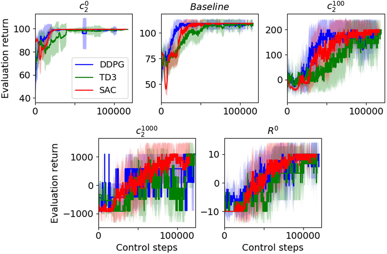
Figure 12. Ensemble average and standard deviation of the evaluation return computed with only trials that led to a winning test trajectory (the average may therefore be performed with different number of runs for each algorithm). The curves were obtained by evaluating the policies at the end of each episode during training.
First, let us focus on cases Baseline (where $ {c}_2=10 $
),
$ {c}_2=10 $
), $ {c}_2^0 $
,
$ {c}_2^0 $
, $ {c}_2^{100} $
,
$ {c}_2^{100} $
, $ {c}_2^{1000} $
, and
$ {c}_2^{1000} $
, and $ {R}^0 $
, leaving aside case
$ {R}^0 $
, leaving aside case $ {R}^{-1} $
. In case
$ {R}^{-1} $
. In case $ {R}^0 $
, a non-null reward is only obtained at the end of the episode if a won or lost situation is reached: the reward is purely sparse. On the opposite side, case
$ {R}^0 $
, a non-null reward is only obtained at the end of the episode if a won or lost situation is reached: the reward is purely sparse. On the opposite side, case $ {c}_2^0 $
features a reward signal that tells the algorithm, at each time step, whether the action has drawn the airfoil closer or farther away from the target; the reward is purely dense. In this last case, the reward model does not fit explicitly the criterion used for evaluating trajectories a posteriori (won when the plate enters the ball of radius
$ {c}_2^0 $
features a reward signal that tells the algorithm, at each time step, whether the action has drawn the airfoil closer or farther away from the target; the reward is purely dense. In this last case, the reward model does not fit explicitly the criterion used for evaluating trajectories a posteriori (won when the plate enters the ball of radius $ \varepsilon $
around point B and lost otherwise). Conversely, the reward model encourages the algorithm to learn how to fly as close as possible to B. Cases Baseline,
$ \varepsilon $
around point B and lost otherwise). Conversely, the reward model encourages the algorithm to learn how to fly as close as possible to B. Cases Baseline, $ {c}_2^{100} $
and
$ {c}_2^{100} $
and $ {c}_2^{1000} $
use a combination of both a dense and a sparse term. The three cases vary in the weight assigned to each term. Among all these cases, the most reliable option when using DDPG or TD3 is the Baseline one, where the sparse term value is approximately 10 to 25% of the sum of the rewards collected, at each time step, over an episode. On the contrary, among the less reliable cases for DDPG and TD3 is the fully sparse
$ {c}_2^{1000} $
use a combination of both a dense and a sparse term. The three cases vary in the weight assigned to each term. Among all these cases, the most reliable option when using DDPG or TD3 is the Baseline one, where the sparse term value is approximately 10 to 25% of the sum of the rewards collected, at each time step, over an episode. On the contrary, among the less reliable cases for DDPG and TD3 is the fully sparse $ {R}^0 $
case. One should note that piecewise constant reward models and deterministic dynamics fall out of the scope of application of deterministic policy gradient algorithms (Silver et al., Reference Silver, Lever, Heess, Degris, Wierstra and Riedmiller2014). DDPG and TD3 belong to this class of algorithms so that they cannot be expected to perform well in sparse reward cases such as
$ {R}^0 $
case. One should note that piecewise constant reward models and deterministic dynamics fall out of the scope of application of deterministic policy gradient algorithms (Silver et al., Reference Silver, Lever, Heess, Degris, Wierstra and Riedmiller2014). DDPG and TD3 belong to this class of algorithms so that they cannot be expected to perform well in sparse reward cases such as $ {R}^0 $
. Besides, even when theoretically applicable, sparse rewards often make the problem hard to solve since they induce a difficult uninformed exploration problem for the RL algorithm. In case
$ {R}^0 $
. Besides, even when theoretically applicable, sparse rewards often make the problem hard to solve since they induce a difficult uninformed exploration problem for the RL algorithm. In case $ {c}_2^{1000} $
, the sparse term is approximately 10 times larger than the sum of the rewards collected over an episode. The dense part might be too low for DDPG and TD3 to perform well. Overall, while DDPG and TD3 are strongly affected by the reward formulations discussed here, SAC is way more robust to these variations, owing to both the regularization term in its objective function and the better exploration process of the stochastic policy.
$ {c}_2^{1000} $
, the sparse term is approximately 10 times larger than the sum of the rewards collected over an episode. The dense part might be too low for DDPG and TD3 to perform well. Overall, while DDPG and TD3 are strongly affected by the reward formulations discussed here, SAC is way more robust to these variations, owing to both the regularization term in its objective function and the better exploration process of the stochastic policy.
Finally, in case $ {R}^{-1} $
, a reward of
$ {R}^{-1} $
, a reward of $ -1 $
is applied at each time step, as well as a sparse term at the end of each episode. Such a formulation defines a signal that directly minimizes the time taken to reach B, but does not inform the behavior policy in terms of progress towards the goal: it boils down to the difficulties of a piecewise constant and sparse reward problem. Indeed, as long as the algorithm does not meet point B at least once by chance, given the data within the replay buffer, the most straightforward way to maximize the return is to minimize the number of time steps per episode by terminating the episode as fast as possible. Interestingly, the policy may therefore remain stuck in a local minimum corresponding to a “suicidal” policy (which terminates each episode as fast as possible), and never explore enough to discover there is a better way to maximize the return. While SAC is more reliable than DDPG or TD3 in all other cases, Table 3 evidences the very poor performance of all three algorithms for case
$ -1 $
is applied at each time step, as well as a sparse term at the end of each episode. Such a formulation defines a signal that directly minimizes the time taken to reach B, but does not inform the behavior policy in terms of progress towards the goal: it boils down to the difficulties of a piecewise constant and sparse reward problem. Indeed, as long as the algorithm does not meet point B at least once by chance, given the data within the replay buffer, the most straightforward way to maximize the return is to minimize the number of time steps per episode by terminating the episode as fast as possible. Interestingly, the policy may therefore remain stuck in a local minimum corresponding to a “suicidal” policy (which terminates each episode as fast as possible), and never explore enough to discover there is a better way to maximize the return. While SAC is more reliable than DDPG or TD3 in all other cases, Table 3 evidences the very poor performance of all three algorithms for case $ {R}^{-1} $
.
$ {R}^{-1} $
.
Changing the reward model implies that different control problems are actually solved, with possibly different optimal trajectories for each scenario. Yet, as in Section 4.2, similar test paths are obtained whatever the reward model (not shown here). Consequently, this benchmark can be used to assess the sample efficiency in regard to the reward model applied. Despite the different scales, cases $ {c}_2^{1000} $
and
$ {c}_2^{1000} $
and $ {R}^0 $
display very similar learning curves in Figure 12. The dense term in the reward of case
$ {R}^0 $
display very similar learning curves in Figure 12. The dense term in the reward of case $ {c}_2^{1000} $
may be too small to be accurately taken into account in the learning so that this case is almost equivalent to the
$ {c}_2^{1000} $
may be too small to be accurately taken into account in the learning so that this case is almost equivalent to the $ {R}^0 $
case. Regarding cases including both a dense and a sparse part, the smaller the sparse term, the quicker the maximum return value is reached (or equivalently, the better the sample efficiency). For all cases presented here, once again, similar learning curves are obtained for DDPG and SAC, whereas TD3 is slower to learn, likely due to its over-caution and delayed updates.
$ {R}^0 $
case. Regarding cases including both a dense and a sparse part, the smaller the sparse term, the quicker the maximum return value is reached (or equivalently, the better the sample efficiency). For all cases presented here, once again, similar learning curves are obtained for DDPG and SAC, whereas TD3 is slower to learn, likely due to its over-caution and delayed updates.
4.4. Variations in the dynamics model
The control problem considered until now has simple dynamics: the environment is deterministic and the task is permissive such that various policies can be quasi-optimal. Now, we investigate the behavior of algorithms in potentially more challenging situations, which could be encountered when moving towards real-world applications. Four different variations from the baseline are considered: decreased actuation frequency, increased airfoil density, added environment noise on the action, and, finally, replacing the low-order model with the resolution of the Navier–Stokes equations to account for unsteady aerodynamic forces. Such variations modify the dynamics of the problem and may therefore alter the learning performance and the associated policy. Both are analyzed in this section.
The first parameter investigated is the control frequency. In this work, this is treated as a tunable parameter. This may not be the case in physical problems that require a specific frequency to control a given phenomenon, or if the goal is to mimic a specific actuation device. Decreasing the actuation frequency leads to a lower-horizon control problem (fewer control steps in each episode) and could therefore induce easier convergence. However, this can hit a threshold frequency under which the problem is under-actuated and no successful policy can be found. The second parameter is the airfoil density. As the density increases, the airfoil inertia increases as well, and the reachable states are increasingly limited. One could then expect that with an increased density, the control problem to solve is harder because the policies have less latitude. Next, environmental noise is added to the action prescribed by the controller: the environment is not deterministic anymore. Note that unlike in robustness studies, here the noise is added during both the learning and testing phases so that the policy learns how to deal with noise. This added noise can resemble the uncertainty in the prescription of the action that can occur in an experimental setting. However, here, the noise value is selected randomly according to a Gaussian distribution centered in zero and of standard deviation $ \sigma \cdot {\dot{\beta}}_0 $
, where
$ \sigma \cdot {\dot{\beta}}_0 $
, where $ \sigma $
is given in Table 4. Note that this is different from the expected noise produced by experimental devices. Nevertheless, this allows a first assessment of the algorithms’ behavior in the presence of environment noise.
$ \sigma $
is given in Table 4. Note that this is different from the expected noise produced by experimental devices. Nevertheless, this allows a first assessment of the algorithms’ behavior in the presence of environment noise.
Table 4. Influence of the transition model: cases characteristics and number of won trials over 20 realizations

Note. Number of won trials smaller or equal to 15 are highlighted in red bold, and black bold when equal to 20.
Finally, the low-order model of the flying flat plate physics used until now is replaced by the resolution of the Navier–Stokes equations with the STAR-CCM+ solver, described in Section 2.1. This introduces more complex dynamics since added mass, virtual camber, and wake effects on the aerodynamic loads are captured, and therefore this case represents a step towards more realistic applications. The state components fed to the RL algorithm are kept unchanged from the low-order model case. As a consequence, the algorithm has now access to only partial information about the complete state describing the underlying MDP: the state observed by the algorithm does not fully describe the environment state, since it has no information on the whole flow fields. This situation leads to ambiguous situations where two identical measurements fed to the policy might actually correspond to two different environment states (e.g., same flat plate position, velocity, and pitch angle, but different surrounding flow field, such as a different unsteady wake topology). Such a control problem moves away from the MDP theoretical framework on which the three analyzed algorithms are built, but also better represents most real-world problems. While the training lasted 1,000 episodes with the low-order model, here, only 500 episodes were performed before testing the controller. This is sufficient to obtain a converged solution and allows to reduce the computational cost of the trials with the high-fidelity model. Besides, a well-known unlearning phenomenon (where the learned policy forgets after being able to perform the task) was observed in a few cases when running the training for longer: a detailed analysis of this phenomenon is beyond the scope of this current work. For all these four variations from the Baseline, Table 4 summarizes the values of the parameters investigated and the corresponding learning reliability, while Figure 13 shows the learning history of some selected cases.

Figure 13. Ensemble average and standard deviation of the evaluation return computed with only trials that led to a winning test trajectory (the average may therefore be performed with different number of runs for each algorithm). The curves were obtained by evaluating the policy at the end of each episode during training.
In case $ {f}^{1/2} $
(respectively,
$ {f}^{1/2} $
(respectively, $ {f}^{1/5} $
), the actuation frequency is decreased compared to the Baseline case: the physical time step
$ {f}^{1/5} $
), the actuation frequency is decreased compared to the Baseline case: the physical time step $ dt $
is kept constant, while the control time step
$ dt $
is kept constant, while the control time step $ \Delta t $
is increased so that
$ \Delta t $
is increased so that $ \Delta t=2 dt $
(respectively,
$ \Delta t=2 dt $
(respectively, $ \Delta t=5 dt $
). As a result, for the same number of episodes, the number of collected samples and neural network updates would be decreased by 2 (respectively, 5). To keep these constant across cases, the number of episodes is increased accordingly so that the total number of collected samples remains of the same order of magnitude. However, this increases the cost associated with sample collection, and, incidentally, with each training trial. Results from Table 4 show that decreasing the control frequency has no significant impact on reliability. However, comparing the curves obtained for the Baseline and the low-frequency actuation case in Figure 13 reveals that a faster learning is achieved for the latter. Indeed, case
$ \Delta t=5 dt $
). As a result, for the same number of episodes, the number of collected samples and neural network updates would be decreased by 2 (respectively, 5). To keep these constant across cases, the number of episodes is increased accordingly so that the total number of collected samples remains of the same order of magnitude. However, this increases the cost associated with sample collection, and, incidentally, with each training trial. Results from Table 4 show that decreasing the control frequency has no significant impact on reliability. However, comparing the curves obtained for the Baseline and the low-frequency actuation case in Figure 13 reveals that a faster learning is achieved for the latter. Indeed, case $ {f}^{1/5} $
is a lower-horizon control problem: the average number of control steps between the initial state and the end of an episode is five times smaller. As a result, the sparse earning at the end of a winning episode is faster to propagate towards initial states, resulting in a faster convergence.
$ {f}^{1/5} $
is a lower-horizon control problem: the average number of control steps between the initial state and the end of an episode is five times smaller. As a result, the sparse earning at the end of a winning episode is faster to propagate towards initial states, resulting in a faster convergence.
To ensure that the global trend obtained when assessing the reliability of the RL algorithms is not specific to the chosen setup, an additional flat plate configuration is tested: case $ {d}^{150} $
corresponds to a different airfoil density compared with Baseline, whose density is
$ {d}^{150} $
corresponds to a different airfoil density compared with Baseline, whose density is $ {d}_s=30\mathrm{kg}\;{\mathrm{m}}^{-3} $
. DDPG and TD3’s reliability slightly decreases when increasing the flat plate density. This is consistent with the fact that the problem is more challenging. Besides, the sample efficiency of DDPG and SAC is not significantly affected, while TD3 requires more samples to converge toward the maximum value of the return.
$ {d}_s=30\mathrm{kg}\;{\mathrm{m}}^{-3} $
. DDPG and TD3’s reliability slightly decreases when increasing the flat plate density. This is consistent with the fact that the problem is more challenging. Besides, the sample efficiency of DDPG and SAC is not significantly affected, while TD3 requires more samples to converge toward the maximum value of the return.
In cases $ {\sigma}^{0.1} $
to
$ {\sigma}^{0.1} $
to $ {\sigma}^{0.75} $
, where environmental noise is added to the action prescribed by the agent, all three algorithms remain reliable whatever the noise intensity. Because the actuation frequency is high, and the noise is random, its average over time equals zero, which yields a null global effect. A correlated noise may lead to different results. Here, the sample efficiency remains similar to that of the Baseline for all three algorithms.
$ {\sigma}^{0.75} $
, where environmental noise is added to the action prescribed by the agent, all three algorithms remain reliable whatever the noise intensity. Because the actuation frequency is high, and the noise is random, its average over time equals zero, which yields a null global effect. A correlated noise may lead to different results. Here, the sample efficiency remains similar to that of the Baseline for all three algorithms.
Finally, in the case of CFD, whatever the algorithm, reliability stays high and sample efficiency is slightly higher, compared to the Baseline. When using RL algorithms in conjunction with CFD solvers, computing the samples is expensive in terms of CPU usage. A trial with the low-order model lasts less than an hour on a single computing core. With the CFD environment, the total computational cost required to perform a trial (RL training and sample collection) is 1,200 times larger. This corresponds to the large CPU time required to collect samples when coupling CFD and RL algorithms, the cost of the RL part being negligible. This significant increase exemplifies the need for reliable and sample-efficient off-policy RL algorithms, which is at the core of the present study.
While the variations in the dynamics model considered here have a limited impact regarding the learning performance, their influence on policies is evidently high. Figure 14a shows all the winning test trajectories and Figure 14b shows the corresponding controller actions, obtained with SAC, for each case presented in Figure 13. Moreover, for each case, in an attempt to compare visually the policies obtained by SAC, TD3, and DDPG, we count how many times each action is taken along a trajectory, and average this count over 20 trials. This provides a probability density function (PDF) of actions along trajectories which is shown in Figure 14c. The trajectories and action signals of the Baseline case obtained with SAC have already been discussed on Figure 10: policies vary a lot from one test to another, but most policies consist in applying a negative pitch rate at the beginning, then stabilizing on average around a value close to zero. Finally, near the end of the episode, close to point B, the different policies cover the whole range of possible values. This leads to the PDF of the actions observed in Figure 14c for SAC, which peaks slightly below zero. The PDFs obtained for DDPG and TD3 are, however, quite different. While a peak below zero can still be observed for DDPG, TD3 evidences a much more evenly distributed pitch rate over the range of possible values. Besides, DDPG and TD3 show a small peak of the PDF at the extrema, which is not observed for SAC. This evidences some periods of action saturation with the former algorithms that are not experienced with SAC. Variations of the PDF are strong between the algorithms for this Baseline case. On the contrary, all three algorithms present similar PDFs for the low frequency actuation case $ {f}^{1/5} $
. Apart from the peaks at the extrema observed only for DDPG and TD3, the PDF curves overlap quite well. Because of the lower control frequency, this case leads to a graphically rougher action sequence signal than the Baseline case but the trajectory envelope is similar. Then, when the plate density is increased, the controller has much less room to maneuver the possible actions at the beginning of the episode. All policies able to reach B consist of applying a significant upward pitch rate from the very beginning until approximately half of the episode. Otherwise, the strong inertia of this case prevents the airfoil from reaching the target. The associated PDF evidences a strong peak close to the minimal pitch rate allowed by the problem. The test trajectories resulting from these resembling policies are very similar. Next, case
$ {f}^{1/5} $
. Apart from the peaks at the extrema observed only for DDPG and TD3, the PDF curves overlap quite well. Because of the lower control frequency, this case leads to a graphically rougher action sequence signal than the Baseline case but the trajectory envelope is similar. Then, when the plate density is increased, the controller has much less room to maneuver the possible actions at the beginning of the episode. All policies able to reach B consist of applying a significant upward pitch rate from the very beginning until approximately half of the episode. Otherwise, the strong inertia of this case prevents the airfoil from reaching the target. The associated PDF evidences a strong peak close to the minimal pitch rate allowed by the problem. The test trajectories resulting from these resembling policies are very similar. Next, case $ {\sigma}^{0.75} $
depicts a very noisy action sequence due to the additional environment noise. However, the actuation frequency is so high that the trajectories are barely affected by the noise and are very similar to that of the Baseline. The three PDF shapes differ from one algorithm to another but they all appear flattened.
$ {\sigma}^{0.75} $
depicts a very noisy action sequence due to the additional environment noise. However, the actuation frequency is so high that the trajectories are barely affected by the noise and are very similar to that of the Baseline. The three PDF shapes differ from one algorithm to another but they all appear flattened.

Figure 14. (a) Trajectory, (b) normalized action $ \dot{\beta}/{\dot{\beta}}_0 $
, and (c) normalized action probability density function (PDF) for selected cases.
$ \dot{\beta}/{\dot{\beta}}_0 $
, and (c) normalized action probability density function (PDF) for selected cases.
Finally, the action sequences in the CFD case are more saturated than in the Baseline case and do not evidence the preference for a negative pitch rate at the beginning of the episode, as observed in all other cases. Instead, the pitch rate values spread over the whole range at the beginning of the episode. The action PDFs are even more flattened than in the noisy case, and do not evidence any pattern apart from the peaks at the extrema already observed for DDPG. Corresponding trajectories are less smooth and way more spread than the ones obtained with the low-order model. This is most likely associated with the richer dynamics involved and the more complex feedback coupling between the airfoil and the fluid when the flow is solved with the Navier–Stokes equations. In particular, because the airfoil can experience large accelerations in pitch, added mass forces (which are not included in the low-order model) are one to two orders of magnitude larger than quasi-steady forces induced by translation, and the controller relies on such forces (rather than quasi-steady forces) to drive the airfoil to point B. In fact, although not shown here for the sake of conciseness, the effective angle of attack can be mostly negative throughout the maneuver, hence mostly producing negative quasi-steady lift. Rather, gain and loss in altitude are correlated with rapid pitch-up and pitch-down (i.e., angular accelerations) of the airfoil. The control strategy is therefore fundamentally different from that obtained with the simplified model, which most likely explains the differences observed in Figure 14. We add that virtual camber and wake effects may also play a role in the control strategy, but their order of magnitude is significantly lower than that of added mass effects. An example of the vorticity field that develops around the airfoil during the maneuver is provided in Appendix A.
4.5. Summary on the sensitivity analysis and reasons to choose SAC over DDPG or TD3
The overall performance of DDPG, TD3, and SAC on the first task in terms of reliability is summarized in Figure 15. For each set of parameters tested in the previous sections, and detailed in Tables 2–4, the percentage of won trials is reported in green as a positive number, and the percentage of lost trials is reported in red as a negative number.

Figure 15 highlights clearly that SAC is more reliable than DDPG and TD3, which both evidence strong reliability variations when parameters vary. On the other hand, SAC is less sensitive to parameter tuning and especially “hard” problems for DRL algorithms (e.g., small network, low replay buffer capacity). The only exception is the $ {R}^{-1} $
case (see Table 3), which leads to catastrophic performance for all three algorithms.
$ {R}^{-1} $
case (see Table 3), which leads to catastrophic performance for all three algorithms.
On this benchmark, and without special optimization of any of the algorithms, SAC was observed to be slightly more CPU consuming than DDPG or TD3 (which is consistent with its inner adjustment mechanisms), but the computational cost gap between algorithms goes to zero when the physics is solved with CFD. Indeed, in such a case, the cost associated to the RL algorithm is negligible compared to the cost associated to the CFD computation.
To sum up, on the first task at hand here, SAC is more reliable, has the same cost when used with CFD, and has a sample efficiency comparable to DDPG and superior than TD3. It is therefore more suitable to set up this new control problem for which we had no prior knowledge in terms of parametrization. The knowledge acquired on this simple task can then be used as a basis when moving towards more complexity.
Interpreting why SAC seems more robust and efficient is an open question in the RL literature, for which we provide some elements here. First, and maybe overall, the entropy regularization term in SAC is known to make the optimization landscape smoother and to drive the optimization more consistently towards the same minima (Geist et al., Reference Geist, Scherrer and Pietquin2019). In the present case, this is reflected through the consistent performance of SAC. Additionally, SAC provides a more principled way of performing exploration, as its behavior policy benefits from an adaptive temperature parameter, while DDPG and TD3 rely on adding Gaussian noise to a deterministic policy. This induces a possibly better coverage of the relevant states and actions, and, in turn, better gradients for the value function and policy. Finally, SAC has been recently analyzed under the lens of robust MDPs (Eysenbach and Levine, Reference Eysenbach and Levine2022) where the policy is optimized to perform well across a span of control problems (instead of a single one). The robustness of SAC policies to variations in the control problem dynamics makes it less sensitive to both environment identification errors and hyperparameter tuning. Nevertheless, SAC and TD3 are mathematically very close (both are approximate value iteration algorithms, using a stochastic behavior policy) and claiming pure dominance of an algorithm over another in RL is a delicate endeavor (Henderson et al., Reference Henderson, Islam, Bachman, Pineau, Precup and Meger2018). Consequently, the take-away message of this section should not be that SAC will always dominate over TD3 or even DDPG. It is actually very likely that there exists a set of hyperparameters for which TD3 or DDPG performs as well or even better than SAC. However, in the present case—and possibly in other fluid dynamics cases such as those studied by Bucci et al. (Reference Bucci, Semeraro, Allauzen, Wisniewski, Cordier and Mathelin2019), Novati et al. (Reference Novati, Mahadevan and Koumoutsakos2019), and Rabault et al. (Reference Rabault, Kuchta, Jensen, Reglade and Cerardi2019) for instance—SAC appears less sensitive to hyperparameter tuning and is thus a good candidate for a fluid dynamics practitioner wishing to set up a new case study.
5. Results for the Second Task: Variable Target Point
The agent is now trained and tested on a more complex task. For this second task, the position of the target point B is drawn randomly in a given domain, as illustrated, at scale, in Figure 16. The domain is a portion of a circular ring revolving around the starting point A, with inner and outer radius, respectively, equal to $ 1.5c $
and
$ 1.5c $
and $ 2.1c $
. The portion corresponds to the
$ 2.1c $
. The portion corresponds to the $ \left[-{8}^{\circ };{8}^{\circ}\right] $
angular interval around the horizontal line.
$ \left[-{8}^{\circ };{8}^{\circ}\right] $
angular interval around the horizontal line.

Figure 16. Illustration (at scale) of the second task: B can take any value in the domain delimited by dashed lines.
After each training episode, an evaluation is performed on a given set of B positions in the domain. Two different sets were tested: one with 11 points as illustrated in Figure 17a and another with 4 points as shown in Figure 17b. This evaluation is used to compare policies on a fairly fixed basis and identify which one leads to the highest return, on average over the evaluation points. This best policy is the one saved and used for testing. Introducing such a metric and saving the best policy according to this metric allows to obtain a quasi-optimal policy even if unlearning happens. Note that this is different from what was done in Section 4, where the policy used for testing was the one obtained at the end of the training (i.e., at the end of the 1,000th [or 500th] episode [for the CFD case]).

Figure 17. Policy evaluation is performed on a given set of B positions in the domain. (a) Set of 11 evaluation positions and (b) set of 4 evaluation positions.
All parameters are kept identical to the Baseline case and the control problem of this second task is defined by the same MDP than the first task: the state and action variables, as well as the reward and transition models, are also kept identical to the Baseline of the first task. At this point, it is interesting to note that
-
• Due to the reward formulation, shorter paths lead to lower returns than longer ones. Or said otherwise, the closer B is to A, the lower the return. The evaluation return is therefore expected to be lower than that of the first task since, on average, the evaluation points are closer to A.
-
• Since the state and reward are defined with respect to B, varying the position of B while keeping the position of A constant is equivalent to varying the position of A while keeping B at the same position.
When analyzing the results obtained with the low-order model on this task, it was observed that the learning speed was very similar for each point of the evaluation set and that the two different sets of evaluation positions led to similar results. For this reason, and to mitigate the cost of the training, only the set of 4 evaluation points is used when training with the high-fidelity model and results are only presented for this case. The best policies obtained for each training are assessed by testing over two different sets of points. First, they are tested with respect to the evaluation points. This is where they are supposed to perform the best, since this is the metric that was used to select the best policies. Then, they are tested over 100 points chosen randomly inside the domain, to analyze their capacity to actually perform the desired task, that is, reach any point in the given domain.
Case characteristics as well as reliability results from the various tests are presented in Table 5. First, for both environments and all algorithms, almost all trials produce policies that successfully reach the evaluation points. Parametrization follows the Baseline one from the first task, for which all three algorithms performed well and while the task is slightly different here, the performance is still nearly perfect for all three algorithms. Interestingly, some of the policies reach all points from the evaluation but fail to reach some locations when tested on 100 random points of the domain. This means that a policy able to meet the metrics requirement does not guarantee that it is actually able to perform the desired task. Choosing the metrics here is a trade-off between evaluation cost (that increases with the number of evaluation points) and accuracy. Note that policies successful on evaluation points but not on all random points missed between 2 and 52 of the 100 points, meaning that some are almost able to perform the task while others perform badly more than half the time. Sample efficiency is then analyzed in Figure 18. DDPG and TD3 keep a similar behavior in this second task, compared to the first one, while SAC is more sample efficient.
Table 5. Second task, variable target point: cases characteristics and number of trials that won on all the target positions tested over 20 trials


Figure 18. Ensemble average and standard deviation of the evaluation return computed with only trials that led to a winning test trajectory (the average may therefore be performed with different number of runs for each algorithm). The curves were obtained by evaluating the policy at the end of each episode during training.
Policies obtained from training on the first and the second tasks are then compared when applied to the target point of the first task. Figure 19a shows the airfoil trajectory and the action obtained with SAC as well as the actions PDFs of all trials that successfully reached the target, for the three algorithms. The trajectory envelope tightens in case $ {Bvar}^{LO} $
compared to the Baseline. Besides, while the PDF curve varies a lot between algorithms in the Baseline, they become very similar in case
$ {Bvar}^{LO} $
compared to the Baseline. Besides, while the PDF curve varies a lot between algorithms in the Baseline, they become very similar in case $ {Bvar}^{LO} $
, with a peak centered in zero. The only notable difference is the peak at the extrema, which is observed only for DDPG and TD3. Note that cases Baseline and
$ {Bvar}^{LO} $
, with a peak centered in zero. The only notable difference is the peak at the extrema, which is observed only for DDPG and TD3. Note that cases Baseline and $ {Bvar}^{LO} $
differ in two ways: (a) the training is performed on a fixed target point versus on a given domain, and (b) the last policy is saved versus the best policy is saved. Case
$ {Bvar}^{LO} $
differ in two ways: (a) the training is performed on a fixed target point versus on a given domain, and (b) the last policy is saved versus the best policy is saved. Case $ {Bvar}^{CFD} $
evidences the same trajectories of envelope tightening compared to its fixed target counterpart in Figure 14. Besides, just like observed in Figure 14, the action trajectories obtained when solving the Navier–Stokes equations spread at the beginning and the pitch rate values cover the full range of possible values instead of the preference for a strong negative pitch rate at the beginning observed when using the low-order model. The effect of such differences in the policies is easily observed in the corresponding trajectories. Interestingly, there is a peak centered at a value close to zero for DDPG and SAC, in place of the flattened PDFs observed when training with CFD on a fixed target point.
$ {Bvar}^{CFD} $
evidences the same trajectories of envelope tightening compared to its fixed target counterpart in Figure 14. Besides, just like observed in Figure 14, the action trajectories obtained when solving the Navier–Stokes equations spread at the beginning and the pitch rate values cover the full range of possible values instead of the preference for a strong negative pitch rate at the beginning observed when using the low-order model. The effect of such differences in the policies is easily observed in the corresponding trajectories. Interestingly, there is a peak centered at a value close to zero for DDPG and SAC, in place of the flattened PDFs observed when training with CFD on a fixed target point.

Figure 19. (a) Trajectory, (b) normalized action $ \dot{\beta}/{\dot{\beta}}_0 $
, and (c) normalized action probability density function (PDF) for selected cases.
$ \dot{\beta}/{\dot{\beta}}_0 $
, and (c) normalized action probability density function (PDF) for selected cases.
To further evaluate the capacities of the policies trained on this second task, they were compared on their ability to reach points outside of the training domain. Results can be found in Appendix B.
6. Conclusion
In this study, three DRL algorithms: DDPG, TD3, and SAC are evaluated and compared regarding reliability and sample efficiency as well as the policies they produce and their generalization capabilities. To do so, a benchmark case, which can be solved by a low-cost low-order approach as well as a high-fidelity CFD approach is proposed. The task consists in controlling an airfoil from an initial point to reach a target. In a first task, the target is kept in a fixed position during the training and testing of the policy, while a second task consists to be able to reach any point in a given domain. The three RL algorithms are evaluated on both tasks when varying the RL hyperparameters, the reward formulation, and the dynamics. We observe that DDPG and TD3’s reliability depends greatly on the RL hyperparameters and the reward formulation, while SAC is more robust to parameter variations and “hard” problems. Besides, the sample efficiency of SAC and DDPG is similar and superior to that of TD3. When testing the algorithms on their generalization capabilities across locations outside the training domain, all algorithms have the same performance. Moreover, their performance is on average improved with CFD compared to the low-order model. Overall, SAC appears both reliable and sample-efficient over a wide range of parametrization setups. It is therefore suited to solve fluid mechanics problems and setup new cases without tremendous effort. In particular, SAC is resistant to small neural networks or replay buffers. The latter is of practical importance if full-flow fields were to be stored. SAC also resists to various reward formulations which are of interest when setting up a new case and even performs well with sparse rewards. Finally, it performs well in situations where optimal policies are unambiguous, that is where there are few optimal action sequences leading to a winning situation (in opposition to situations where several very different sequences enable reaching the goal).
Regarding the parameter variations analyzed in this study, while the sample efficiency varies a lot with all parameters, the reliability is mostly affected by RL hyperparameters and reward formulation but not so by dynamics. Interestingly, the successful parametrization identified on the low-order model proved successful with the CFD environment: DDPG, TD3, and SAC are all reliable and sample efficient in this case. This means that a preliminary study can be performed on a cheaper version for this case. Unlike reliability and sample efficiency, policies are barely impacted by RL hyperparameters and reward formulation but evidently vary a lot with dynamics. In particular, while policies keep the same global pattern across tasks, the overall strategy employed when RL algorithms are coupled to the low-order model is quite different than that produced when using the CFD solver. This limits the possibility of transferring a policy learned on the low-order model to directly apply it in the CFD. Some preliminary tests have been performed in that way and did not prove successful. Such a transfer would be of tremendous interest since it would reduce the CPU cost of learning. This can be viewed (for instance) under the prism of curriculum learning for RL, where a sequence of learning contexts of increasing difficulty is defined by adding representative features (and the corresponding samples) in the dynamics model, which closes the gap towards a more physically realistic environment. In such a framework, fine-tuning with few samples, a policy that was pre-trained on a computationally cheap low-order model, is yet a challenge for future research, which would constitute a major step forward for the applicability of RL to fluid mechanics problems.
Acknowledgments
The authors acknowledge the support from CALMIP for HPC resources.
Author contribution
Conceptualization: S.B., T.J., E.R., M.B.; Funding acquisition: M.B.; Investigation: S.B.; Methodology: S.B., T.J., E.R., M.B.; Software: S.B., A.A.R., V.G., T.L., B.M.; Validation: S.B.; Visualization: S.B.; Writing–Original Draft: S.B.; Writing–Review and Editing: T.J., E.R., M.B. All authors approved the final submitted draft.
Competing interest
The authors declare none.
Data availability statement
The entire code used to obtain the results presented in this article is available on GitHub. In order to facilitate the reproducibility of our results without requiring an in-depth understanding of the code, each case study is stored in a separate repository containing all the necessary code and setup to execute the case directly. The code for the following tasks can be found in the respective repositories:
-
• First task with fixed target and low-order model: https://github.com/SuReLI/aerobench_fixed_target_low_order.
-
• First task with fixed target and CFD model: https://github.com/SuReLI/aerobench_fixed_target_star.
-
• Second task with variable target and low-order model: https://github.com/SuReLI/aerobench_variable_target_low_order.
-
• Second task with variable target and CFD model: https://github.com/SuReLI/aerobench_variable_target_star.
Funding statement
This research was supported by the French Ministry of Defense through the DGA/AID. The funder had no role in study design, data collection and analysis, decision to publish, or preparation of the manuscript.
A. Vorticity fields along the airfoil trajectory in the CFD-DRL framework
Figure A1 displays instantaneous vorticity snapshots obtained at four instants during a maneuver performing the first task (i.e., fixed starting and target points). The action sequence of this maneuver is obtained by testing one of the 20 policies obtained for the 20 trials performed with SAC for the CFD case discussed in Section 4.4. At t = 0 s, the plate has its pitch axis located on A. The flow around the plate is characterized by two thick, opposite-sign shear layers that advect into the wake. At t = 0.00078 s, the plate has pitched up while traveling towards B. The pitch-up motion has caused the positive (blue) vorticity layer to roll up into a counter-clockwise rotating vortex. The subsequent pitch-down motion then caused the vortex to shed into the wake and promoted the generation of a clockwise rotating vortex. Alternate shedding of clockwise and counter-clockwise rotating vortices is also observed later in the maneuver, at time t = 0.0017 s. These structures, together with wake oscillations, are the only clear footprint of pitch-up/pitch-down motions defined by the controller once the plate has reached B at t = 0.00234 s. That is, for this specific task, there is no evidence of leading edge flow separation that could promote more aggressive maneuvers through additional vortex lift, for example.

Figure A1. Instantaneous vorticity field at various time steps of the CFD-DRL framework applied to the trajectory control of an airfoil going from point A to point B. The action sequence of this maneuver is obtained by testing one of the 20 policies obtained for the 20 trials performed with SAC for the CFD case discussed in Section 4.4.
B. Out-of-domain generalization capabilities of the trained policies
The policies trained on the second task are compared to their ability to reach points outside of the training domain. These points are all taken at the same $ x=-2c $
, while their
$ x=-2c $
, while their $ y $
coordinate is varied to move the point further away from the training domain. Results are presented in Table B1.
$ y $
coordinate is varied to move the point further away from the training domain. Results are presented in Table B1.
Table B1. Generalization capabilities on the second task, variable target point: number of won trials over 20 realizations

Generalization capabilities for points outside the domain are very random but globally decrease with distance to the training domain. However, symmetrical points with respect to the horizontal do not lead to the same reliability, indicating that it is not only a matter of distance. Interestingly, the policies trained with CFD are more robust than those trained with the low-order model.


 Open access
Comments
No Comments have been published for this article.