


Impact Statement
The availability of monitoring data from engineering structures offers many opportunities for optimizing their design and operation. The ability to be able to predict the current health state of a structure, for example, opens the door to predictive maintenance and, in turn, enhanced safety and reduced cost and waste. Currently most attempts at harnessing knowledge within collected datasets are reliant on those data alone, limiting the potential of what can be done to how much of the entire life of a structure is captured. This paper demonstrates how using physical knowledge within a machine learning approach can improve predictions considerably, reducing the burden on expensive data collection. A range of approaches allow differing levels/types of physical insight to be incorporated.
1. Data versus physics: an opinionated introduction
The umbrella term data-centric engineering, and interest in it, results from our growing ability and capacity to collect data from our built environment and engineered systems. The potential gains from being able to harness the information in these data are large, attracting many researchers and practitioners to the field. Here we enjoy the very engaging challenge of simultaneously assessing what we think we know, what we can measure, and what might actually tell us about the particular structure or system we are interested in.
As our data grow, many researchers naturally look to adopt machine learning (ML) methods to help analyze and predict behaviors of interest in our measured systems. Within this vibrant field, there are many advances with the potential to enhance or optimize how we design and operate our human-made world. The drivers and challenges of taking a data-driven approach in an engineering setting are often, however, different for those developing the latest ML/AI algorithms. Generalizing significantly, where a ML practitioner might look to develop a powerful algorithm that can make predictions across many applications without user input, an engineer’s interest may necessarily be more system-focused and should also consider what knowledge can be gained from the model itself alongside optimizing its predictive capability. In terms of challenges, one of the most significant is simply that engineering data, although sometimes “big,” often do not capture all behaviors of interest, may consist of indirect measurements of those behaviors, and, for operational monitoring, will often be noisy, corrupt, or missing.
To give an example where these challenges are particularly pertinent, consider the problem of asset management of civil infrastructure. Given a fixed budget for a monitoring system, we’d like to be able to collect and use data to tell us something about the current condition of a structure (or multiple structures). Ultimately we’d really like to be able to use that data to make predictions about how the structure(s) will perform in the future. As a monitoring system comes online, the data available may be large in size; however, the information content in it will be limited by the operational conditions seen in the monitoring window, the current condition of the structure, and the robustness of the sensing and acquisition system. A data-driven model established in this setting bears the same limitations and we should be careful (and are) about how we expect any such model to generalize to future structural and operational conditions.
Many have and will question why pursuing a data-driven approach is interesting in this context given these limitations/challenges, especially considering our efforts and successes throughout history in understanding and describing the world and beyond via physics. The blunt answer is that we don’t know everything, and, when we do know enough, modeling complex (multi-physics, multi-scale) processes interacting with a changing environment is often difficult and energy-consuming. The more compelling answer, perhaps, is that we would really like any inferences we make to be based on the evidence of what is happening currently, and for that, observation is needed.
Given a particular context, there are, of course, benefits and disadvantages in taking either approach; a physics-based one can provide interpretability, parsimony, and the ability to extrapolate, for example, whereas data-driven approaches can be considered more flexible, may require less user input, and take into account evidence from latest measurements. The selected route may come down to personal choice but hopefully is the result of a reasoned argument.
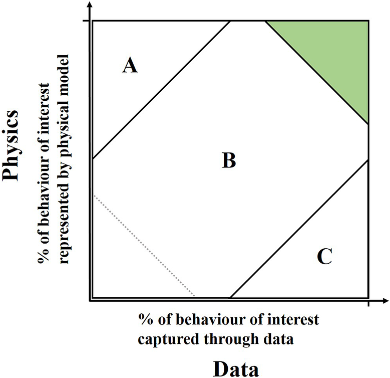
One hypothetical approach to this reasoning may be to consider how much of the process of interest can be described by known/modeled physics (within a given computational budget) versus how much of it can be characterized by available data (supposing one could assess such things); see Figure 1. Broadly speaking, in region A one would likely take a physics-based approach and in region C a data-driven one. In the happy green area, either may be applicable, and in the bottom left-hand corner, one may wish to consider the best route to gain additional knowledge, whether through measurement or otherwise (the triangle sizes here are arbitrary and for illustration only).
Mapping of problem settings according to knowledge available from physical insight and data.
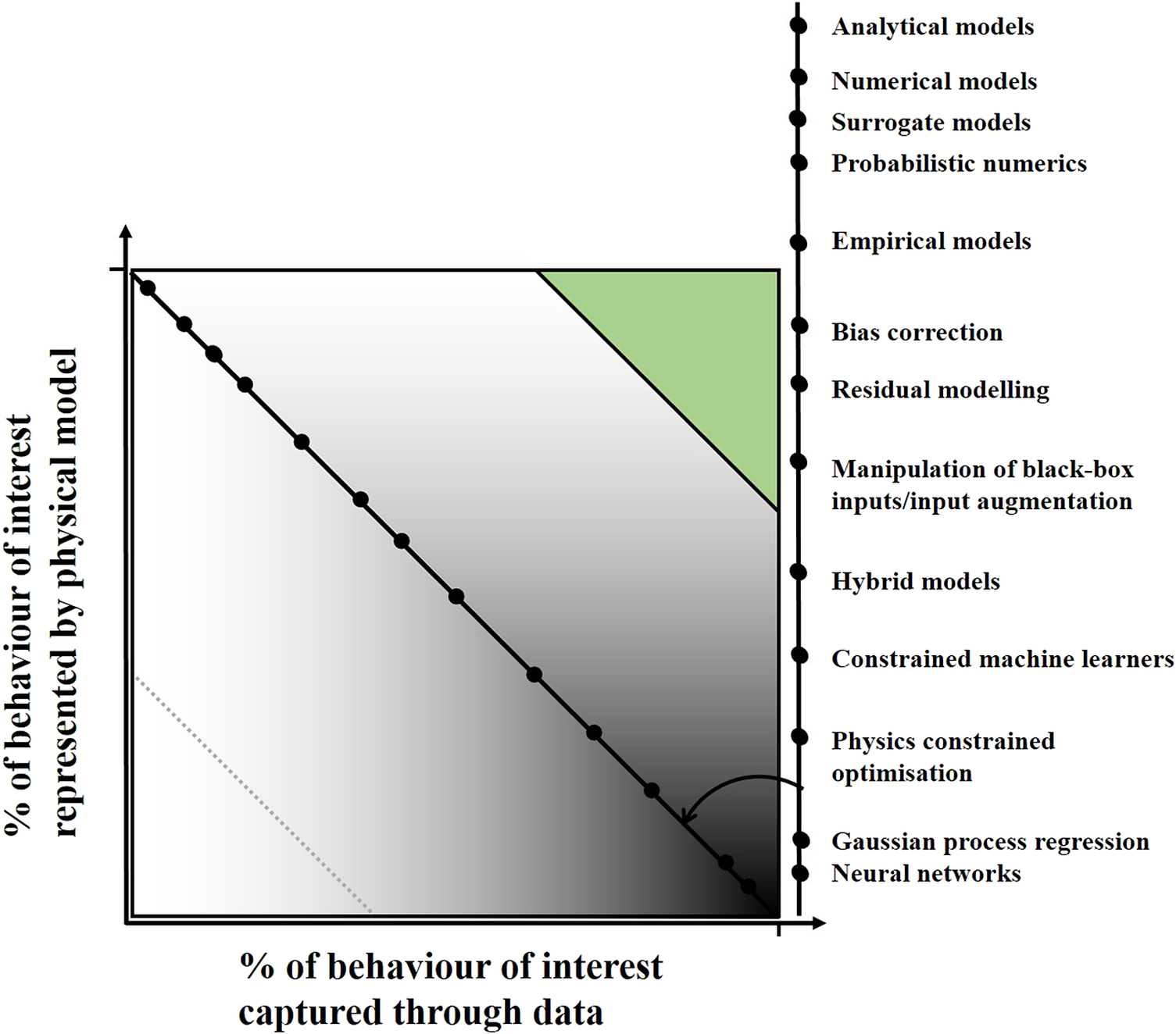
Recently interest has been growing in methods that attempt to exploit physics-based models and evidence from data together, hopefully retaining the helpful attributes from both approaches. Indeed, there has been an explosion of literature on these methods in the past few years, duly reviewed in Willard et al. (Reference Willard, Jia, Xu, Steinbach and Kumar2020), Karniadakis et al. (Reference Karniadakis, Kevrekidis, Lu, Perdikaris, Wang and Yang2021), and von Rueden et al. (Reference von Rueden, Mayer, Beckh, Georgiev, Giesselbach, Heese, Kirsch, Pfrommer, Pick, Ramamurthy, Walczak, Garcke, Bauckhage and Schuecker2023). These methods should be useful for the many engineering problems that fall in region B (in Figure 1, the gray area). “Gray” is also occasionally used to describe the models themselves, alluding to them being a mix of physics (so-called white-box) and data-driven (so-called black-box) approaches. The term “physics-informed machine learning” is now also commonly used for those methods at the darker end of the scale.
Figure 2 very loosely maps some of the available methods that exist in the modeling community onto the knowledge from physics and data axes from the original figure and the black to white spectrum (of course it must be noted here that method location will change according to the specific model type and how it is applied—sometimes significantly so). At the lighter end of the scale, surrogate models are a continually growing area of interest (Kennedy and O’Hagan, Reference Kennedy and O’Hagan2001; Queipo et al., Reference Queipo, Haftka, Shyy, Goel, Vaidyanathan and Tucker2005; Bhosekar and Ierapetritou, Reference Bhosekar and Ierapetritou2018; Ozan and Magri, Reference Ozan and Magri2022) where emulation of an expensive-to-run physical model is needed. The emerging field of probabilistic numerics (Cockayne et al., Reference Cockayne, Oates, Sullivan and Girolami2019; Hennig et al., Reference Hennig, Osborne and Kersting2022) attempts to account for uncertainty within numerical modeling schemes and overlaps with communities specifically looking at bias correction and residual modeling (Arendt et al., Reference Arendt, Apley and Chen2012; Brynjarsdottir and Hagan, Reference Brynjarsdottir and Hagan2014; Gardner et al., Reference Gardner, Rogers, Lord and Barthorpe2021), where a data-driven component is used to account for error in a physical model in the first case, or behaviors not captured by a physical model in the latter (most often achieved by summing contributions from both elements). In the middle sit methods where there is a more even share between the explanatory power of physics and data-driven components; this may simply be achieved by feeding the predictions of a physical model into a machine learner as inputs (Fuentes et al., Reference Fuentes, Cross, Halfpenny, Worden and Barthorpe2014; Rogers et al., Reference Rogers, Holmes, Cross and Worden2017; Worden et al., Reference Worden, Barthorpe, Cross, Dervilis, Holmes, Manson and Rogers2018), or may involve a more complicated architecture informed by understanding of the process itself. Examples of these hybrid models include neural networks where the interaction between neurons and the design of their activation functions reflect knowledge of the physics at work in the situation to be modeled (Cai et al., Reference Cai, Mao, Wang, Yin and Karniadakis2021; Lai et al., Reference Lai, Mylonas, Nagarajaiah and Chatzi2021). Finally at the blacker end of the scale sit constrained methods where, for example, laws or limits can be built into a machine learner to aid optimization or ensure physically feasible predictions. Many studies in this area focus on constraining a cost function (Karpatne et al., Reference Karpatne, Atluri, Faghmous, Steinbach, Banerjee, Ganguly, Shekhar, Samatova and Kumar2017; Cai et al., Reference Cai, Mao, Wang, Yin and Karniadakis2021), for example, parameter optimization, with fewer focusing on directly constraining the model itself (as will be the case in a part of this work) (Wahlström et al., Reference Wahlström, Kok, Schön and Gustafsson2013; Jidling et al., Reference Jidling, Hendriks, Wahlström, Gregg, Schön, Wensrich and Wills2018; Solin et al., Reference Solin, Kok, Wahlström, Schön and Särkkä2018; Jones et al., Reference Jones, Rogers and Cross2023).
A non-exhaustive list of modeling approaches very loosely mapped onto the data/physics problem setting axes from Figure 1.
This paper considers a spectrum of models from white to black under a Gaussian process (GP) prior assumption. GPs have been shown to be a powerful tool for regression tasks (Rasmussen and Williams, Reference Rasmussen and Williams2006), and their use in this context within engineering is becoming common (see, e.g., Kullaa, Reference Kullaa2011; Avendaño-Valencia et al., Reference Avendaño-Valencia, Chatzi, Koo and Brownjohn2017; Wan and Ni, Reference Wan and Ni2018, Reference Wan and Ni2019). The regular use of GP regression by the authors of this paper (e.g., Cross, Reference Cross2012; Holmes et al., Reference Holmes, Sartor, Reed, Southern, Worden and Cross2016; Bull et al., Reference Bull, Gardner, Rogers, Cross, Dervilis and Worden2020; Rogers et al., Reference Rogers, Worden and Cross2020) is because of their simple ability to function given small datasets and, importantly, the Bayesian framework within which they naturally work; the predictive distribution provided allows the calculation of useful confidence intervals and the opportunity for uncertainty to be propagated forward into any following analysis (see, e.g., Gibson et al., Reference Gibson, Rogers and Cross2020). Despite these advantages, their use in the provided citations remains entirely data-driven and thus open to the challenges/limitations discussed above.
By drawing an explicit link between the classical treatment of GPs in physical sciences and how they are used for regression in an ML context, this paper illustrates a derivation path for a spectrum of possible GP models suitable for incorporating differing levels of physical insight. To do so, Section 2 introduces GPs from both perspectives, with Section 3 identifying their overlap and the specific means of incorporating physical insight into a GP regression. Examples of specific models across the spectrum developed for structural assessment are demonstrated in Section 4. Established models that appear on the spectrum from related fields are discussed below and also in the concluding section (Section 5), which also attempts to use the studies highlighted here to give insight into applicability and future directions.
1.1. Related work
The past several years have seen an increase in the use of physics-informed GPs across a variety of research fields. Arguably the simplest construction of physics-informed GPs has been those based on residual modeling, where a GP learns the difference between measured data and that of a physics-derived model, for instance, a finite element analysis or an analytical approximation of the phenomena at play. In Pitchforth et al. (Reference Pitchforth, Rogers, Tygesen and Cross2021), a residual-based model is formulated for predicting wave loading on an offshore structural member, combining a simplified, semi-empirical law with a GP regression. In some research communities, residual modeling is also referred to as bias correction, where the belief is that model parameters can be updated to reflect the information of measured data via a correction function, which Chen et al. (Reference Chen, Xiong, Tsui and Wang2008) represented as a GP. In Wan and Ren (Reference Wan and Ren2015, Reference Wan and Ren2016) similar strategies are proposed for updating a finite element model for identifying the modal properties of large-scale civil infrastructure.
Input augmentation is also a means of utilizing the outputs of a physical model in combination with a GP.Footnote 1 To form such a model, the outputs of the physical model are augmented with the observational data and used as additional inputs to the machine learner. Input augmentation has offered performance gains for modeling cascaded tanks exhibiting nonlinear behavior (Rogers et al., Reference Rogers, Holmes, Cross and Worden2017) and optimizing hydroelectric power generation (Sohlberg and Sernfält, Reference Sohlberg and Sernfält2002). Parts of the system identification community also categorize transformation to inputs of a black-box model as semi-physical modeling (Lindskog and Ljung, Reference Lindskog and Ljung1994).
Another area that has combined physics and GPs is in the modeling of ordinary and partial differential equations (ODE/PDEs). In the work of Pförtner et al. (Reference Pförtner, Steinwart, Hennig and Wenger2022), GPs conditioned on observations resulting from linear operators are shown to provide a general framework for solving linear PDEs, accommodating scenarios where physics are partially known (i.e., the full governing equations are unavailable), as well as propagating error resulting from both parameter and measurement uncertainty. In a similar vein, Raissi et al. (Reference Raissi, Perdikaris and Karniadakis2017a, Reference Raissi, Perdikaris and Karniadakis2018) and Raissi and Karniadakis (Reference Raissi and Karniadakis2018) demonstrate that by constructing a joint distribution between successive time or spatial points, a GP prior can be constructed that can explicitly learn solutions of partial differential equations, coining the term “numerical Gaussian processes.”
Other GP works that have sought to leverage governing equations are those of latent force models (LFMs), which integrate driving mechanistic laws to infer unknown inputs (Alvarez et al., Reference Alvarez, Luengo and Lawrence2009). In Hartikainen and Särkkä (Reference Hartikainen and Särkkä2010), state space formulations of LFMs address the computational burden of direct inference over LFMs. Here the covariance function is reconstructed as a solution to a linear time-invariant stochastic differential equation, an approach now adopted for some problems in the structural dynamics community (Nayek et al., Reference Nayek, Chakraborty and Narasimhan2019; Rogers et al., Reference Rogers, Worden and Cross2020). Attention has also been given to treating nonlinear latent force models (Ward et al., Reference Ward, Ryder, Prangle and Alvarez2020). In Beckers et al. (Reference Beckers, Wu and Pappas2023), an interesting step is taken of combining LFMs with a variational autoencoder for learning the dynamics of a moving object from a video sequence, where, unlike in much of the previously referenced works, the resulting GP posterior is not Gaussian, due to the use of a Bernoulli likelihood for the pixel observation model. For modeling wind turbine power curves, Mclean et al. (Reference Mclean, Jones, O’Connell, Maguire and Rogers2023) also performed inference over a non-Gaussian physics-informed GP, where a Beta likelihood observation model was chosen to reflect prior understanding that the normalized predicted power output cannot exceed one, which is the maximum rated power.
Moving toward physics-informed GPs that generally are more data-driven in nature, constrained GPs serve as a general term for a GP whose predictions satisfy some imposed condition(s); a comprehensive overview can be found in Swiler et al. (Reference Swiler, Gulian, Frankel, Safta and Jakeman2020). Given that knowledge of a constraint will likely arise in the context of physical insight, such GP models fall firmly into the realm of physics-informed. For instance, in modeling a degradation process, one may wish to enforce a monotonicity constraint (Riihimäki and Vehtari, Reference Riihimäki and Vehtari2010; Agrell, Reference Agrell2019). In Haywood-Alexander et al. (Reference Haywood-Alexander, Dervilis, Worden, Cross, Mills and Rogers2021) a series of kernels is constructed that embed differing aspects of physical characteristics to model ultrasonic-guided waves. The inclusion of both differential equations (Alvarez et al., Reference Alvarez, Luengo and Lawrence2009; Raissi and Karniadakis, Reference Raissi and Karniadakis2018; Long et al., Reference Long, Wang, Krishnapriyan, Kirby, Zhe and Mahoney2022)Footnote 2 and boundary conditions (Cross et al., Reference Cross, Gibbons and Rogers2019; Jones et al., Reference Jones, Rogers and Cross2023) through constraining predictions via an appropriate operator over the kernel has also been considered.
2. GPs from a physics and ML perspective
2.1. Physics-based perspective
From a classical perspective, a GP is one example in a wider family of stochastic processes used to characterize randomness. To begin to describe a stochastic process intuitively, one can consider something that evolves through time. In this case, a stochastic process is one where, at each instance of time, $ t $
, the value of the process is a random variable. In characterizing the stochastic process, we are describing the evolution of probability distributions through time. Note that we may equally wish to consider the evolution of a process through a variable (
$ t $
, the value of the process is a random variable. In characterizing the stochastic process, we are describing the evolution of probability distributions through time. Note that we may equally wish to consider the evolution of a process through a variable ( $ \in {\mathrm{\mathbb{R}}}^n $
) that is not time, and will do so later in the paper.
$ \in {\mathrm{\mathbb{R}}}^n $
) that is not time, and will do so later in the paper.
The fundamental elements for describing a stochastic process are the mean and autocorrelation, which are functions over time (or the input variable(s) of interest). Considering a process $ y(t) $
, its mean
$ y(t) $
, its mean $ \mu (t) $
and autocorrelation
$ \mu (t) $
and autocorrelation $ \phi \left({t}_1,{t}_2\right) $
functions are
$ \phi \left({t}_1,{t}_2\right) $
functions are
 $$ {\displaystyle \begin{array}{c}\mu (t)=\unicode{x1D53C}\left[y(t)\right]\\ {}\phi \left({t}_1,{t}_2\right)=\unicode{x1D53C}\left[y\left({t}_1\right)y\left({t}_2\right)\right]\\ {}={\int}_{-\infty}^{\infty }{\int}_{-\infty}^{\infty }y\left({t}_1\right)y\left({t}_2\right)g\left(y\left({t}_1\right),y\left({t}_2\right)\right) dy\left({t}_1\right) dy\left({t}_2\right),\end{array}} $$
where $ \unicode{x1D53C} $
is the expectation operator. The autocorrelation requires integration of the product of
$ \unicode{x1D53C} $
is the expectation operator. The autocorrelation requires integration of the product of $ y\left({t}_1\right)y\left({t}_2\right) $
and their joint probability density,
$ y\left({t}_1\right)y\left({t}_2\right) $
and their joint probability density, $ g $
, at times
$ g $
, at times $ {t}_1 $
and
$ {t}_1 $
and $ {t}_2 $
(this is sometimes referred to as the second-order density).
$ {t}_2 $
(this is sometimes referred to as the second-order density).
Following on from this, the (auto)covariance of a process, $ k\left({t}_1,{t}_2\right) $
, is
$ k\left({t}_1,{t}_2\right) $
, is
 $$ k\left({t}_1,{t}_2\right)=\unicode{x1D53C}\left[\left(y\left({t}_1\right)-\mu \left({t}_1\right)\right)\left(y\left({t}_2\right)-\mu \left({t}_2\right)\right)\right]. $$
Clearly, the autocorrelation and (auto)covariance are one and the same for a process with a zero mean.
A GP is one where at each instance or iteration the value of the variable of interest follows a normal/Gaussian distribution, with the joint distribution of a finite collection of these also normal. It is completely defined by its mean and the covariance function, that is, one need only consider the joint density between two points (second-order density).
Many of the behaviors/variables that we wish to model in science and engineering are stochastic processes. The first use of the term “stochastic process” arose in the 1930s (Doob, Reference Doob1934; Khintchine, Reference Khintchine1934), but the response of a physical system to random excitation, which is most certainly a stochastic process, had been under study since at least the turn of the 20th century.Footnote 3
A particular example of interest that will be used later in this paper is that of a structure vibrating. Perhaps the simplest formulation of a stochastic process in this context is the response of a deterministic system under random excitation. Generally speaking, if the excitation to a linear dynamical system is a GP, then the response of that system is also a GP (a GP remains a GP under linear operations; Papoulis and Pillai, Reference Papoulis and Pillai2002).
Given an assumed equation of motion (or physical law of interest) for $ y $
, one can attempt to derive the covariance function of a process using (1, 2). Later in the paper the derived covariance function for a single degree of freedom (SDOF) system under random loading will be shown and employed in a GP regression setting.
$ y $
, one can attempt to derive the covariance function of a process using (1, 2). Later in the paper the derived covariance function for a single degree of freedom (SDOF) system under random loading will be shown and employed in a GP regression setting.
2.2. Data-driven perspective
In the context of GP regression, that is, from a data-driven perspective, the process is unknown (to be learned from data), and so the definition of the mean and covariance functions become a modeling choice. These choices form the prior mean and covariance, which will be updated to the posterior mean and covariance given the observations of the process of interest.
An example of a common choice for covariance function is the squared exponential (SE) with an additional white noise covariance term:
 $$ k\left({\mathbf{x}}_p,{\mathbf{x}}_q\right)={\sigma}_y^2\exp \left(-\frac{1}{2{l}^2}{\left\Vert {\mathbf{x}}_p-{\mathbf{x}}_q\right\Vert}^2\right)+{\sigma}_n^2{\delta}_{pq}. $$
Rather than a process through time, $ t $
, this is a covariance function for a process defined over a multivariate input space with elements
$ t $
, this is a covariance function for a process defined over a multivariate input space with elements $ {\mathbf{x}}_i $
(reflecting the more generic nature of regression tasks attempted). Here there are three hyperparameters:
$ {\mathbf{x}}_i $
(reflecting the more generic nature of regression tasks attempted). Here there are three hyperparameters: $ {\sigma}_y^2 $
, the signal variance;
$ {\sigma}_y^2 $
, the signal variance; $ l $
, the length scale of the process; and
$ l $
, the length scale of the process; and $ {\sigma}_n^2 $
, the variance from the noise on the measurements. This may be easily adapted to allow a separate length scale for each input parameter if required.
$ {\sigma}_n^2 $
, the variance from the noise on the measurements. This may be easily adapted to allow a separate length scale for each input parameter if required.
After selection of appropriate mean and covariance functions and with access to measurements of the process of interest, the regression task is achieved by calculating the conditional distribution of the process at testing points given the observations/measurements.
Following the notation used in Rasmussen and Williams (Reference Rasmussen and Williams2006), $ k\left({\mathbf{x}}_p,{\mathbf{x}}_q\right) $
defines a covariance matrix
$ k\left({\mathbf{x}}_p,{\mathbf{x}}_q\right) $
defines a covariance matrix $ {K}_{pq} $
, with elements evaluated at points
$ {K}_{pq} $
, with elements evaluated at points $ {\mathbf{x}}_p $
and
$ {\mathbf{x}}_p $
and $ {\mathbf{x}}_q $
, where
$ {\mathbf{x}}_q $
, where $ {\mathbf{x}}_i $
may be multivariate.
$ {\mathbf{x}}_i $
may be multivariate.
Assuming a zero-mean function, the joint Gaussian distribution between measurements/observations $ \mathbf{y} $
with inputs
$ \mathbf{y} $
with inputs $ X $
and unknown/testing targets
$ X $
and unknown/testing targets $ {\mathbf{y}}^{\ast } $
with inputs
$ {\mathbf{y}}^{\ast } $
with inputs $ {X}^{\ast } $
is
$ {X}^{\ast } $
is
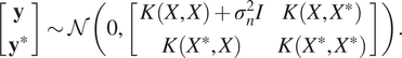 $$ \left[\begin{array}{c}\mathbf{y}\\ {}{\mathbf{y}}^{\ast}\end{array}\right]\sim \mathcal{N}\left(0,\left[\begin{array}{cc}K\left(X,X\right)+{\sigma}_n^2I& K\left(X,{X}^{\ast}\right)\\ {}K\left({X}^{\ast },X\right)& K\left({X}^{\ast },{X}^{\ast}\right)\end{array}\right]\right). $$
The distribution of testing targets $ {\mathbf{y}}^{\ast } $
conditioned on the training data (which is what we use for prediction) is also Gaussian:
$ {\mathbf{y}}^{\ast } $
conditioned on the training data (which is what we use for prediction) is also Gaussian:
 $$ {\displaystyle \begin{array}{ll}{\mathbf{y}}^{\ast}\mid {X}_{\ast },X,\mathbf{y}\sim \mathcal{N}& \Big(K\left({X}^{\ast },X\right){\left(K\left(X,X\right)+{\sigma}_n^2I\right)}^{-1}\mathbf{y},\hskip0.35em \\ {}& K\left({X}^{\ast },{X}^{\ast}\right)-K\left({X}^{\ast },X\right){\left(K\left(X,X\right)+{\sigma}_n^2I\right)}^{-1}K\left(X,{X}^{\ast}\right)\Big)\end{array}}. $$
See Rasmussen and Williams (Reference Rasmussen and Williams2006) for the derivation. The mean and covariance here are that of the posterior GP.
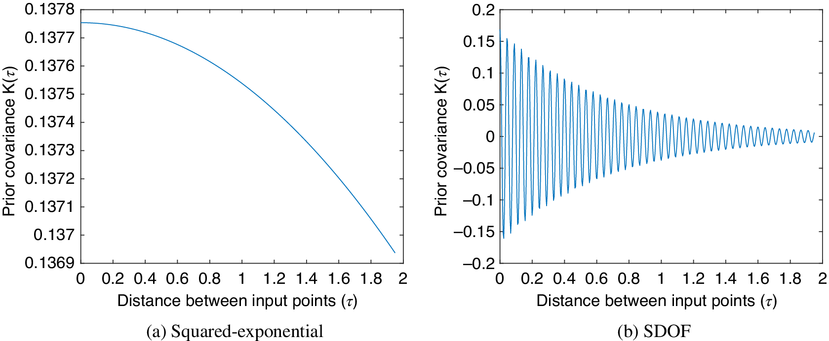
From equation (5)) one can see that the GP mean prediction at point $ {\mathbf{x}}^{\ast } $
is simply a weighted sum—determined by the covariance function—of training points
$ {\mathbf{x}}^{\ast } $
is simply a weighted sum—determined by the covariance function—of training points $ \mathbf{y} $
. Figure 3a illustrates how the influence of a training point on a prediction decays as the distance in the input space increases when using the SE covariance function (hyperparameters arbitrarily selected). This shows how the covariance between points with similar inputs will be high, as is entirely appropriate for a data-based learner. In the absence of training data in an area of the input space, the mean value of GP will return to the prior mean (usually zero). An equivalent plot for the covariance function of an SDOF oscillator employed later (Section 4) is included for comparison, where one can see the oscillatory nature captured.
$ \mathbf{y} $
. Figure 3a illustrates how the influence of a training point on a prediction decays as the distance in the input space increases when using the SE covariance function (hyperparameters arbitrarily selected). This shows how the covariance between points with similar inputs will be high, as is entirely appropriate for a data-based learner. In the absence of training data in an area of the input space, the mean value of GP will return to the prior mean (usually zero). An equivalent plot for the covariance function of an SDOF oscillator employed later (Section 4) is included for comparison, where one can see the oscillatory nature captured.
Measure of influence of an input point on a prediction for the squared exponential (a) and the covariance function of single degree of freedom (SDOF) oscillator under a random load (b).
3. A spectrum of GPs for regression
Commonly engineering applications of GP regression will follow a typical ML approach and adopt a zero mean prior and a generic covariance function selected from either the SE or the Matérn kernel class (Rasmussen and Williams, Reference Rasmussen and Williams2006). In an upcoming summary figure, this will be denoted as $ f(x)\sim \mathcal{GP}\left(0,{k}_{\mathrm{ML}}\right) $
, with
$ f(x)\sim \mathcal{GP}\left(0,{k}_{\mathrm{ML}}\right) $
, with $ \mathrm{ML} $
denoting the ML approach as above. Although successful in many settings, these applications suffer from those same challenges discussed in the introduction, namely that the regression bears the same limitations as the dataset available with which to characterize the system/structure of interest.
$ \mathrm{ML} $
denoting the ML approach as above. Although successful in many settings, these applications suffer from those same challenges discussed in the introduction, namely that the regression bears the same limitations as the dataset available with which to characterize the system/structure of interest.
Here the incorporation of one’s physical insight of a system into a GP regression is introduced as a means of lessening reliance on complete data capture. The GP framework provides a number of opportunities to account for physical insight, the biggest coming from the definition of the prior mean and covariance functions. Following on from the previous section, perhaps the most obvious approach is to use physically derived mean and covariance functions where available (equations (1)) and (2)). If these can be derived, they may readily be used in the regression context, denoted as $ f(x)\sim \mathcal{GP}\left({\mu}_P,{k}_P\right) $
(
$ f(x)\sim \mathcal{GP}\left({\mu}_P,{k}_P\right) $
( $ P $
stands for physics).
$ P $
stands for physics).
This section lays out a number of modeling options for a more likely scenario that one has partial knowledge of the system of interest. Following the flow from more physical insight to less, each of the models discussed is placed on the white to black spectrum in Figure 4, perhaps giving an indication of the kind of problem where they may be most usefully employed (illustrative examples of each follow in the next section). As with Figure 2, it should be noted that how each model type is developed and applied could change its placement on the spectrum.
A spectrum of GPs for regression combining physics-derived mean and covariance functions, $ {\mu}_P,{k}_P $
, with those more standardly used in ML,
$ {\mu}_P,{k}_P $
, with those more standardly used in ML, $ {k}_{ML} $
.
$ {k}_{ML} $
.
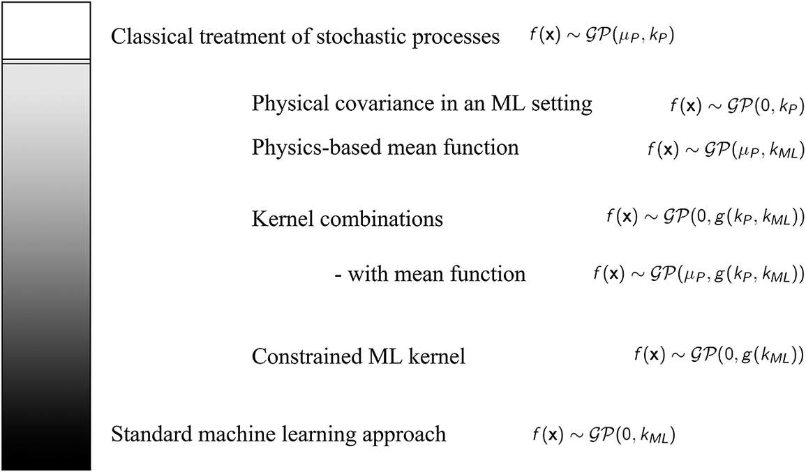
Light gray: If one is able to express the mean behavior of the process of interest, or something close to the mean, then this is easily accounted for by employing that mean as a prior with a standard ML covariance function to capture the variability around it: $ f(x)\sim \mathcal{GP}\left({\mu}_P,{k}_{\mathrm{ML}}\right) $
(Zhang et al., Reference Zhang, Rogers and Cross2020; Pitchforth et al., Reference Pitchforth, Rogers, Tygesen and Cross2021). If the form of the differential equation governing the process of interest is known along with the covariance derivable, then this may also simply be used in place of the data-driven kernels discussed above,
$ f(x)\sim \mathcal{GP}\left({\mu}_P,{k}_{\mathrm{ML}}\right) $
(Zhang et al., Reference Zhang, Rogers and Cross2020; Pitchforth et al., Reference Pitchforth, Rogers, Tygesen and Cross2021). If the form of the differential equation governing the process of interest is known along with the covariance derivable, then this may also simply be used in place of the data-driven kernels discussed above, $ f(x)\sim \mathcal{GP}\left(0,{k}_P\right) $
(Cross and Rogers, Reference Cross and Rogers2021). In this case, the learning of unknown system parameters may be achieved by maximizing the marginal likelihood,
$ f(x)\sim \mathcal{GP}\left(0,{k}_P\right) $
(Cross and Rogers, Reference Cross and Rogers2021). In this case, the learning of unknown system parameters may be achieved by maximizing the marginal likelihood, $ p\left(y|X\right) $
, in the way that one learns the hyperparameters in the standard ML approach (see, e.g., Rasmussen and Williams, Reference Rasmussen and Williams2006).
$ p\left(y|X\right) $
, in the way that one learns the hyperparameters in the standard ML approach (see, e.g., Rasmussen and Williams, Reference Rasmussen and Williams2006).
Medium gray: In the more likely scenario of only possessing partial knowledge of the governing equations of a system of interest, or not being able to derive a covariance analytically, the suggestion here is that the GP prior may be approximated or formed as a combination of derived and data-driven covariance functions so that the data-driven component accounts in some way for unknown behavior; $ f\left(\mathbf{x}\right)\sim \mathcal{GP}\left(0,g\left({k}_P,{k}_{\mathrm{ML}}\right)\right) $
, for some function
$ f\left(\mathbf{x}\right)\sim \mathcal{GP}\left(0,g\left({k}_P,{k}_{\mathrm{ML}}\right)\right) $
, for some function $ g $
, or perhaps
$ g $
, or perhaps $ f\left(\mathbf{x}\right)\sim \mathcal{GP}\left({\mu}_P,g\left({k}_P,{k}_{\mathrm{ML}}\right)\right) $
if a mean may be appropriately approximated.
$ f\left(\mathbf{x}\right)\sim \mathcal{GP}\left({\mu}_P,g\left({k}_P,{k}_{\mathrm{ML}}\right)\right) $
if a mean may be appropriately approximated.
Although this is an area very much still under investigation, the suggested route here is to begin, if possible, by considering or assuming the likely interaction between the known and unknown behaviors and to propagate this through to the prior GP structure. For example, say that one can assume that the response of a structure is a sum of understood behavior and an unknown contribution; $ y=A+B $
, with
$ y=A+B $
, with $ A $
known and
$ A $
known and $ B $
unknown, then the autocorrelation of this process can be formed as
$ B $
unknown, then the autocorrelation of this process can be formed as
 $$ \unicode{x1D53C}\left[y{y}^{\prime}\right]=\unicode{x1D53C}\left[\left(A+B\right)\left({A}^{\prime }+{B}^{\prime}\right)\right]=\unicode{x1D53C}\left[A{A}^{\prime }+A{B}^{\prime }+{A}^{\prime }B+B{B}^{\prime}\right]. $$
If $ A $
and
$ A $
and $ B $
may be assumed to be independent and we make the standard ML prior assumption on
$ B $
may be assumed to be independent and we make the standard ML prior assumption on $ B $
of a zero mean and covariance
$ B $
of a zero mean and covariance $ {K}_B $
, this suggests a suitable GP modelFootnote
4 would be
$ {K}_B $
, this suggests a suitable GP modelFootnote
4 would be $ y\sim \mathcal{GP}\left(0,{K}_A+{K}_B\right) $
. As any linear operation between covariance functions is valid, this route is available for many likely scenarios in an engineering setting where the response to be modeled is a convolution between a known system and unknown force (as will be the case for the derived covariance in the first example below), or a product between a known temporal response and an unknown spatial one (
$ y\sim \mathcal{GP}\left(0,{K}_A+{K}_B\right) $
. As any linear operation between covariance functions is valid, this route is available for many likely scenarios in an engineering setting where the response to be modeled is a convolution between a known system and unknown force (as will be the case for the derived covariance in the first example below), or a product between a known temporal response and an unknown spatial one ( $ y=A(t)B(x)\Longrightarrow y\sim \mathcal{N}\left(0,{K}_A(t)\times {K}_B(x)\right) $
, for
$ y=A(t)B(x)\Longrightarrow y\sim \mathcal{N}\left(0,{K}_A(t)\times {K}_B(x)\right) $
, for $ x $
and
$ x $
and $ t $
independent).
$ t $
independent).
Dark gray: Finally, if the physical insight one has is perhaps more general or cannot be expressed through a mean or covariance function, one can consider adapting a data-driven covariance function to obey known constraints or laws. This may be done by, for example, the construction of a multiple-output GP with auto and cross-covariance terms designed to reflect our knowledge (Wahlström et al., Reference Wahlström, Kok, Schön and Gustafsson2013; Jidling et al., Reference Jidling, Hendriks, Wahlström, Gregg, Schön, Wensrich and Wills2018), or by constraining predictions onto a target domain such that boundary conditions on a spatial map can be enforced (Solin and Kok, Reference Solin and Kok2019; Jones et al., Reference Jones, Rogers and Cross2023).
The next section shows examples for each of these categories, with discussion following in Section 5. Each of the examples is presented quite briefly, with references for further reading. The intention, and the reason for brevity, is to attempt to illustrate models across the range of spectra with conclusions drawn from them jointly in Section 5.
4. Examples
4.1. Physics-derived means and covariances
The light gray models described above are applicable when one can derive an approximate mean or covariance function for the process of interest.
Example 1. $ f\left(\mathbf{x}\right)\sim \mathcal{GP}\left(0,{k}_P\right). $
In Section 2, an oscillatory system under white noise was used as an example of GP in time. For an SDOF, the equation of motion is $ m\ddot{y}(t)+c\dot{y}(t)+ ky(t)=F(t) $
, with
$ m\ddot{y}(t)+c\dot{y}(t)+ ky(t)=F(t) $
, with $ m $
,
$ m $
, $ c $
,
$ c $
, $ k $
, and
$ k $
, and $ F $
being the mass, damping, stiffness, and force, respectively. Under a white noise excitation of variance
$ F $
being the mass, damping, stiffness, and force, respectively. Under a white noise excitation of variance $ {\sigma}^2 $
, one can derive the (auto)covariance of the response
$ {\sigma}^2 $
, one can derive the (auto)covariance of the response $ Y(t) $
;
$ Y(t) $
; $ {\phi}_{Y\left({t}_1\right)Y\left({t}_2\right)}=\unicode{x1D53C}\left[Y\left({t}_1\right)Y\left({t}_2\right)\right] $
, which is solvable either via some lengthy integration or by Fourier transform of the power spectral density (Cross and Rogers, Reference Cross and Rogers2021):
$ {\phi}_{Y\left({t}_1\right)Y\left({t}_2\right)}=\unicode{x1D53C}\left[Y\left({t}_1\right)Y\left({t}_2\right)\right] $
, which is solvable either via some lengthy integration or by Fourier transform of the power spectral density (Cross and Rogers, Reference Cross and Rogers2021):
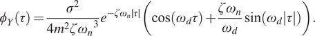 $$ {\phi}_Y\left(\tau \right)=\frac{\sigma^2}{4{m}^2{{\zeta \omega}_n}^3}{e}^{-{\zeta \omega}_n\mid \tau \mid}\left(\cos \left({\omega}_d\tau \right)+\frac{{\zeta \omega}_n}{\omega_d}\sin \left({\omega}_d|\tau |\right)\right). $$
Here standard notation has been used; $ {\omega}_n=\sqrt{k/m} $
, the natural frequency;
$ {\omega}_n=\sqrt{k/m} $
, the natural frequency; $ \zeta =c/2\sqrt{km} $
, the damping ratio;
$ \zeta =c/2\sqrt{km} $
, the damping ratio; $ {\omega}_d={\omega}_n\sqrt{1-{\zeta}^2} $
, the damped natural frequency; and
$ {\omega}_d={\omega}_n\sqrt{1-{\zeta}^2} $
, the damped natural frequency; and $ \tau ={t}_i-{t}_j $
(this is a stationary process).
$ \tau ={t}_i-{t}_j $
(this is a stationary process).
If one has a system that behaves similarly to this, then we may readily use such a covariance function in a regression context. Figure 5 shows the prediction of an undersampled SDOF system using a GP regression with this covariance function, compared to one with a more standard kernel in an ML setting (the SE). The crosses mark the training/conditioning points.
Comparison between the prediction of GPs with squared exponential and SDOF kernels when conditioned on every 10th point of simulated vibration data (Cross and Rogers, Reference Cross and Rogers2021). The gray area indicates confidence intervals (CI) at three standard deviations.
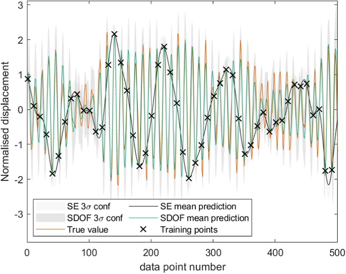
Hyperparameters for both models were learned from maximizing the marginal likelihood, $ p\left(y|X\right) $
,Footnote
5 with the hyperparameters of the SDOF kernel being the parameters
$ p\left(y|X\right) $
,Footnote
5 with the hyperparameters of the SDOF kernel being the parameters $ {\omega}_n,\zeta $
of the system itself. The hyperparameters of the standard SE kernel are the length scale and signal variance.
$ {\omega}_n,\zeta $
of the system itself. The hyperparameters of the standard SE kernel are the length scale and signal variance.
One can see that the GP with the standard covariance function (labeled as SE) smooths through the observed data as designed, and that the GP with the derived covariance function (labeled as SDOF mean prediction) is much more appropriately equipped to model the process than its purely data-driven counterpart. In particular, the inbuilt frequency content of the derived covariance function gives a significant advantage ( $ {w}_n $
is learned as a hyperparameter within a bounded search space).
$ {w}_n $
is learned as a hyperparameter within a bounded search space).
In giving the kernel structure pertinent to the process of interest, one is able to significantly reduce reliance on conditioning data, in this case allowing sampling below Nyquist. This covariance function will also be employed in a later example with extension to multiple degrees of freedom.
Example 2. $ f(x)\sim \mathcal{GP}\left({\mu}_P,{k}_{\mathrm{ML}}\right). $
In some situations, the mean behavior of a process may be broadly understood. This example shows the prediction of deck displacement of a stay-cabled bridge,Footnote 6 the model of which is intended for use in monitoring the structure performance. Deck displacement is a function of a number of factors, principally traffic loading and temperature. Considering physical insight, we believe that the general displacement trend is driven by the contraction and relaxation of the cables with temperature, with seasonal trends visible. Here, therefore, a good candidate prior mean function is a linear relationship between cable extension and temperature.
Figure 6 compares two standard GP regressions (with SE covariance functions) with and without the prior mean function included. Mimicking the case where data from a full monitoring campaign is only available over a short time window, the models are trained (conditioning and hyperparameter setting) using data from the first month of the 5-month period shown. As before, and indeed in all following examples, the SE hyperparameters (length scale and signal and noise variance) are found through maximizing the marginal likelihood, $ p\left(y|X\right) $
. The GP with a zero mean prior (top image in Figure 6) is unable to accurately predict the deck displacement mean-wise as the temperature drops seasonally toward the end of the 5-month period (as this is an unseen condition, as indicated by the increased confidence interval).
$ p\left(y|X\right) $
. The GP with a zero mean prior (top image in Figure 6) is unable to accurately predict the deck displacement mean-wise as the temperature drops seasonally toward the end of the 5-month period (as this is an unseen condition, as indicated by the increased confidence interval).
Comparison between GPs predicting bridge deck displacement over time with prior mean of zero above and with physics-informed mean function below (Zhang et al., Reference Zhang, Rogers and Cross2020).
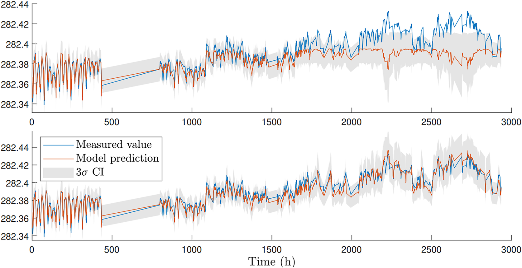
In this case, building in the linear relationship between cable extension and temperature as a prior mean function allows a more successful extrapolation into the colder months (lower image in Figure 6), again demonstrating a lessened reliance on complete data for training.
4.2. Combined derived and data-driven covariance functions
In the middle of the spectra are the many problems where governing equations are only available to describe some of the behaviors of interest. The hybrid models here are proposed to account for this, with the interaction between physical and data-driven components necessarily more interwoven.
Example 3. $ f\left(\mathbf{x}\right)\sim \mathcal{GP}\left(0,g\left({k}_P,{k}_{\mathrm{ML}}\right)\right). $
The motivating problem here is the health/usage monitoring of an aircraft wing during flight, where we would like to predict wing displacement spatially and temporally to feed into a downstream fatigue damage calculation (Holmes et al., Reference Holmes, Sartor, Reed, Southern, Worden and Cross2016; Gibson et al., Reference Gibson, Rogers and Cross2023). In this case, one could assume that the solution of the equation of motion has separable spatial and temporal components, as with a cantilever beam. Under a random load, the covariance of the temporal component may be derived as in Example 1 (assuming linearity), accounting for multiple degrees of freedom by adding covariance terms up for each of the dominant modes (see Pitchforth et al., Reference Pitchforth, Rogers, Tygesen and Cross2022). As the wing will likely be complex in structure, a data-driven model component (covariance) is a good candidate to account for spatial variation.Footnote
7 With separability, the covariance of the process will be a product between the spatial and temporal components, which would make the assumed GP model: $ y\sim \mathcal{GP}\left(0,{K}_{\mathrm{MDOF}}(t){K}_{\mathrm{ML}}(x)\right) $
.
$ y\sim \mathcal{GP}\left(0,{K}_{\mathrm{MDOF}}(t){K}_{\mathrm{ML}}(x)\right) $
.
Figure 7 shows a simple illustration of this using a simulated cantilever beam under an impulse load—assuming here that we have no prior knowledge of the likely form of the spatial (modal) response. The GP is conditioned on a subsampled and truncated time history (1:2:T) from eight points spatially distributed across the beam. The performance of the model in capturing the spatial temporal process is assessed by decomposing the beam response into its principal modes and comparing reconstruction errors across 100 spatial points and the full time history of the simulation (1:end). Figure 7 shows the GP prediction of the first two modes, where one can see that fidelity in the spatial and temporal domains is good.
Hybrid covariance structure modeling the spatiotemporal behavior of a vibrating beam—the spatial variation is assumed to be unknown. The predictions of the model are decomposed into the principal modes of the beam and shown here spatially (a,b) and temporally (c,d) for the first two modes. Normalized mean squared errors spatially are 0.002 and 0.225 (log loss –5.472,–3.088), with time domain errors 0.411 and 0.285 (log loss –3.520,–2.677) respectively (Pitchforth et al., Reference Pitchforth, Rogers, Tygesen and Cross2022).

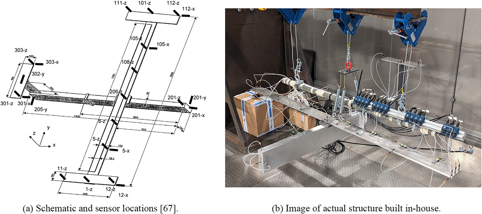
Having demonstrated good performance on a simulated case study, a second example more representative of a real-world scenario was considered in the form of a benchmark aircraft structure built to simulate the behavior of an airplane. Initially designed by the Group for Aeronautical Research and Technology in EURope (GARTEUR) to exhibit the dynamic behavior similar to that of a real aircraft, the structure has since been used as a benchmark for dynamic model validation studies and for assessing modal identification and model updating methods (Balmes and Wright, Reference Balmes and Wright1997; Link and Friswell, Reference Link and Friswell2003; Xia and Lin, Reference Xia and Lin2004; Govers and Link, Reference Govers and Link2010; Delo et al., Reference Delo, Surace, Worden and Brennan2023). A detailed description of the structure can be found in Link and Friswell (Reference Link and Friswell2003). Figure 8 shows an image of the authors’ in-house GARTEUR structure, as well as a schematic detailing the location of the sensors. The data used for demonstration here are the measurements of the aircraft response under a random load between 4 and 80 Hz, with the challenge again being able to make spatial-temporal predictions of the response of the structure. For this example, seven spatial locations of interest are across the span of both wings; these are sensors 1-z, 5-z, 8-z, 206-z, 108-z, 105-z, and 101-z, shown in Figure 8.
Images of benchmark GARTEUR aircraft. Note that the experimental setup used and shown here in (b) does not include the wing tips from the original benchmark configuration shown in (a).
As before, a GP with an SDOF covariance function (from Example 1) in product with a more standard covariance (SE) to account for the unknown spatial variation is used. Training on every sixth time point, Figure 9 shows the corresponding predictions made at each of the sensors along the span of the wing over 1,500 time points, where it can be seen that the model is able to accurately account for both the spatial and temporal component of the response of the aircraft structure.
Predictions of the spatial-temporal response of GARTEUR, decomposed into the temporal prediction at each sensor. The top plot corresponds to sensor 1-z, with each successive plot the next sensor along the span of the wing. The normalized mean squared error averaged across all sensors is 5.18 (log loss –1.45). It is worthwhile highlighting that without including sensor 206-z, the averaged error reduces to 0.62 (log loss –1.43). The reduced performance at this location is likely explained by sensor 206-z being at a node (little response). The log loss remains largely unchanged as the full predictive posterior is reflective of the variation on the measurements.

Knowledge of the system has been used in two ways here, firstly in developing the model structure (the kernel product) and secondly in accounting for the time domain behavior through derived covariance. The relative importance of each is dependent on the availability of training data. Where fully sampled temporal and spatial data are available, a black-box counterpart should be comparable in performance so long as the selected covariance is sufficiently flexible/expressive. Knowledge of the separability of the domains has allowed good prediction here where limited data are available spatially, with the temporal knowledge becoming important where data are not fully sampled in time.
4.3. Constrained covariance functions
At the darkest end of the spectrum are problems and models where insights may be more general in nature, particularly where that knowledge cannot be used to derive generative equations.
Example 4. $ f\left(\mathbf{x}\right)\sim \mathcal{GP}\left(0,g\left({k}_{\mathrm{ML}}\right)\right). $
This example looks at the problem of crack localization in a complex structure using acoustic emission monitoring (acoustic emissions occur during the initialization and growth of cracks, which may be detected and located through high-frequency sensing; Jones et al., Reference Jones, Rogers, Worden and Cross2022; Jones, Reference Jones2023). The task central to the localization is to attempt to learn a map of how energy propagates through a structure from any possible crack location to a number of fixed sensors that are deployed to monitor acoustic emissions. The map is created by introducing a forced acoustic burst at each possible crack location (with a laser or pencil lead break) and then, in our case, producing an interpolative model that can be used inversely to infer location when a new emission is recorded. A large restriction limiting the use of such a localization scheme is the need to collect training data across the structure, which can be time-consuming and costly. Similarly, from a physical perspective, propagation of AE through a structure is complex (and costly) to model unless that structure is homogenous and of simple geometry. The proposed solution here is to follow a data-driven approach but with inbuilt information of the geometry/boundaries of the system, hopefully helping with both shortcomings.
Figure 10 shows how the use of a constraint to a standard ML covariance function can considerably lessen reliance on full data capture. Here a localization map has been made of AE propagation through a plate with a number of holes; and a standard GP is compared to one where knowledge of the boundaries of the plate has been built into a sparse approximation of the covariance function, which reformulates the kernel as an eigen decomposition of the Laplacian of the plate domain (Jones et al., Reference Jones, Rogers and Cross2023). The two approaches perform similarly where training data are abundant, but we begin to see the gains of the introduced boundaries as training grid density decreases, and particularly so when parts of the plate are not mapped at all in the training phase.
Comparison of standard and constrained GP models for AE crack localization (Jones et al., Reference Jones, Rogers and Cross2023) where training data have been limited to the middle section of the plate. (a) Compares model errors at decreasing training grid densities, with measurements at the boundaries included (top), partial boundary measurements (middle), and no boundary measurements (bottom). (b) Shows an example of squared error difference between the two models across the plate, with the standard GP showing increased errors away from the training area.

5. Discussion and conclusions
Each of the examples shown here has demonstrated how the introduction of physical insight into a GP regression has lessened reliance on conditioning data and has shown significantly increased model performance over black-box examples where training data are incomplete.
The number of ways of accounting for knowledge within the GP framework provides parsimonious means to capture many of the different forms of prior knowledge that engineers possess and, in some cases, particularly when employing a mean function can be quite simply achieved.
An additional benefit of many of the models shown is enhanced interpretability, which is particularly important in the applied setting. In Examples 1 and 3, the hyperparameters of the GP are the physical parameters of the system itself, opening the door to system identification in some cases.
Of the methods introduced/discussed, some are more familiar than others. The use of a mean function here takes the same approach as the bias correction community when a GP regression is used to account for discrepancy between a physical (often numerical) model and measurements of the real system (Kennedy and O’Hagan, Reference Kennedy and O’Hagan2001; Gardner et al., Reference Gardner, Rogers, Lord and Barthorpe2021). Underlying the application shown here is the unspoken assumption that physics built into the mean function is trusted, thus allowing the consideration of extrapolation. Although the flexibility of the GP means that it is well able to account for potential bias, in its presence and in the case of incomplete data available for training, one is as unable to place trust in the model across the operational envelope as one would be in the black-box case. In the case of incomplete data, this would suggest that only the simplest physics of which one is confident should be built into the regression.
The design of useful kernels is also naturally an area of interest for many, although often for different purposes than those explored here. Covariance design has been considered within the control community to improve the performance of machine learners for system identification tasks (Ljung, Reference Ljung2010; Pillonetto and Nicolao, Reference Pillonetto and Nicolao2010; Schoukens and Ljung, Reference Schoukens and Ljung2019). In Pillonetto et al. (Reference Pillonetto, Dinuzzo, Chen, Nicolao and Ljung2014) a review is provided in this context, where the focus is on the derivation of a covariance function that will act as an optimal regularizer for the learning of linear dynamical system parameters. Within the ML community, researchers attempting to develop more generic technology also look to physical systems to provide covariance functions useful for a broad class of problems (Higdon, Reference Higdon2002; Boyle and Frean, Reference Boyle and Frean2005; Alvarez et al., Reference Alvarez, Luengo and Lawrence2009; Wilson and Adams, Reference Wilson and Adams2013; Tobar et al., Reference Tobar, Bui and Turner2015; Parra and Tobar, Reference Parra and Tobar2017; Van der Wilk et al., Reference Van der Wilk, Rasmussen and Hensman2017; McDonald and Álvarez, Reference McDonald and Álvarez2021; Ross et al., Reference Ross, Smith and Álvarez2021). These examples present very flexible models that are able to perform very well for a variety of different tasks. As discussed in the introduction, the motivation here is to build in system-specific knowledge to lessen reliance on data capture. These models will only help with tasks where the physics that inspired the general model is representative of the process of interest.
Including pertinent physical insight in a GP regression has most commonly been achieved via the multiple output framework, where relationships between multivariate targets are encoded in cross-covariance terms, including those studies already mentioned while discussing constraints (Wahlström et al., Reference Wahlström, Kok, Schön and Gustafsson2013; Jidling et al., Reference Jidling, Hendriks, Wahlström, Gregg, Schön, Wensrich and Wills2018; Solin et al., Reference Solin, Kok, Wahlström, Schön and Särkkä2018). In Cross et al. (Reference Cross, Gibbons and Rogers2019) we adopt a multiple output GP to constrain a predictor using knowledge of physical boundary conditions for a structural health-monitoring task.a more comprehensive approach in this context is shown, where the relationships between monitored variables are captured with the multiple output framework; different combinations of covariance functions are also considered. Notable contributions relevant here and also applied within an engineering context (Raissi et al., Reference Raissi, Perdikaris and Karniadakis2017a, Reference Raissi, Perdikaris and Karniadakis2017b, Reference Raissi, Perdikaris and Karniadakis2018) use a differential operator to constrain multiple outputs to represent a system of differential equations. All of these works, which show significant improvement over an entirely black-box approach, adapt the standard ML covariance functions commonly used for regression. Expanding the possibility of directly derived priors in both mean and covariance as done here provides an opportunity (where available) to improve these models further.
The hybrid methods discussed in the medium (murky) gray section have been less well studied in this context and are the subject of ongoing work. The more complex interactions between physical and data-driven components have the potential to provide powerful models, although their use and interpretability will depend on architecture. When combining covariance functions over the same input domain, for example, the flexibility of the data-driven component will generally mean that hopes of identifiability are lost, while nonetheless still preserving predictive power.
Finally, across disciplines, there are a growing number of examples now available demonstrating how knowledge of the boundaries or constraints of a system can be very helpful in the automated learning of their corresponding mapping (Coveney et al., Reference Coveney, Corrado, Roney, O’Hare, Williams, O’Neill, Niederer, Clayton, Oakley and Wilkinson2020; Swiler et al., Reference Swiler, Gulian, Frankel, Safta and Jakeman2020), with many of the multiple output GP examples discussed above falling in this category. The flexibility of such models, alongside the opportunity to build in the simplest of intuitions, will likely prove very popular in the future.
The main aim of this work was to provide a spectrum of potential routes to account for differing levels of physical insight within a regression context, using a GP framework. The examples employed here have demonstrated how the derivation path proposed can allow one to establish simple yet flexible models with components and/or (hyper)parameters linked to the physical system. This has been shown to be a desirable pursuit when models must be established without an abundance of training data—a common occurrence across engineering applications, where monitoring of our key infrastructure remains a difficult and expensive challenge.
Acknowledgments
The authors would like to thank Keith Worden for his general support and feedback on this manuscript. Additionally, thanks is offered to James Hensman, Mark Eaton, Robin Mills, Gareth Pierce, and Keith Worden for their work in acquiring the AE dataset used here. We would like to thank Ki-Young Koo and James Brownjohn in the Vibration Engineering Section at the University of Exeter for providing us data regarding the Tamar Bridge.
Author contribution
E.J.C.: conceptualization (lead), methodology (equal), validation (equal), formal analysis (equal), investigation (equal), data curation (equal), writing—original draft (lead), writing—review and editing (lead), supervision (lead), funding acquisition (lead). T.J.R.: methodology (equal), validation (supporting), formal analysis (supporting), investigation (supporting), data curation (supporting), writing—review and editing (supporting), supervision (supporting). D.J.P.: methodology (equal), validation (equal), formal analysis (equal), investigation (equal), data curation (equal), writing—review and editing (supporting). S.J.G.: methodology (equal), validation (supporting), formal analysis (supporting), investigation (supporting), data curation (supporting), writing—review and editing (supporting). S.Z.: methodology (supporting), formal analysis (supporting), investigation (supporting), data curation (equal). M.R.J.: methodology (equal), validation (equal), formal analysis (equal), investigation (equal), data curation (equal), writing—review and editing (supporting).
Competing interest
The authors confirm that no competing interests exist.
Data availability statement
Data availability is not applicable to this article as no new data were created or analyzed in this study.
Funding statement
The authors would like to acknowledge the support of the EPSRC, particularly through grant reference number EP/S001565/1, and Ramboll Energy for their support to S.J.G. and D.J.P.


 Open access
Comments
No Comments have been published for this article.