
1 MOTIVATION AND INTRODUCTION
In recent years, spatial econometric models have become increasingly popular in investigating spillover effects or competition in various fields of economics, including but not limited to tax competition (Lockwood and Migali, Reference Lockwood and Migali2009; Lyytikäinen, Reference Lyytikäinen2012, Baskaran, Reference Baskaran2014), the relationship between democracy and economic growth (Acemoglu et al., Reference Acemoglu2019), the impact of social networks on education (Calvó-Armengol, Patacchini, and Zenou, Reference Calvó-Armengol, Patacchini and Zenou2009; Liu and Lee, Reference Liu and Lee2023), and international trade (Lee, Yang, and Yu, Reference Lee, Yang and Yu2023). The spatial autoregressive (SAR) model is one of the most prevalent models in this area. Correspondingly, several estimation methods have been proposed and thoroughly studied for the SAR model, including quasi maximum likelihood estimation (QMLE), two-stage least squares (2SLS) estimation, the best instrumental variable (IV) estimation, the generalized method of moments (GMM), etc. The estimation methods mentioned above work well when the disturbances are short-tailed distributed, but are very sensitive to outliers or long-tailed disturbances. Our simulation studies reveal that these classical estimators tend to possess large variances in such circumstances. However, data with outliers or long-tailed disturbances are prevalent in economics and finance, e.g., housing prices, students’ academic grades, income, yield rates of stocks or other financial assets, and the air quality index. As an example, this article employs an SAR model to investigate the housing prices in Beijing and documents that the estimated disturbances are long-tailed. This observation motivates us to develop some robust estimation methods for the SAR model that can better handle such scenarios.
This article is inspired by the Huber M-estimation proposed in Huber (Reference Huber1964), one of the mainstream robust estimation methods. An M-estimator is defined as
 $\arg \min _{\theta }\frac {1}{n}\sum _{i=1}^{n}\rho (x_{i},\theta )$
, where
$\arg \min _{\theta }\frac {1}{n}\sum _{i=1}^{n}\rho (x_{i},\theta )$
, where
 $\rho (\cdot )$
is a loss function. It is well known that least squares estimators are not robust to outliers and long-tailed disturbances for linear regression models. Huber (Reference Huber1964) combines the square loss function and the absolute value loss function to form a new loss function. M-estimators based on this loss function enjoy the merits of both least squares estimators and least absolute deviation (LAD) estimators, i.e., it is robust to outliers and more efficient than LAD estimators. The original Huber M-estimators are based on the assumption that regressors are exogenous. A few researchers manage to develop Huber-type estimators that accommodate endogeneity. Wagenvoort and Waldmann (Reference Wagenvoort and Waldmann2002) extend the idea of generalized M-estimators in Mallows (Reference Mallows1975) to develop two robust estimators for a linear model in the presence of endogeneity, namely, the two-stage generalized M-estimator (2SGM) and robust GMM estimator, respectively.Footnote
1
Kim and Muller (Reference Kim and Muller2007) generalize 2SLS estimation to the two-stage Huber estimation for a linear regression model with endogenous regressors. Sølvsten (Reference Sølvsten2020) proposes an estimator that is robust to outliers in a linear model with many IVs. All the works above deal with linear regression models with independent data.
$\rho (\cdot )$
is a loss function. It is well known that least squares estimators are not robust to outliers and long-tailed disturbances for linear regression models. Huber (Reference Huber1964) combines the square loss function and the absolute value loss function to form a new loss function. M-estimators based on this loss function enjoy the merits of both least squares estimators and least absolute deviation (LAD) estimators, i.e., it is robust to outliers and more efficient than LAD estimators. The original Huber M-estimators are based on the assumption that regressors are exogenous. A few researchers manage to develop Huber-type estimators that accommodate endogeneity. Wagenvoort and Waldmann (Reference Wagenvoort and Waldmann2002) extend the idea of generalized M-estimators in Mallows (Reference Mallows1975) to develop two robust estimators for a linear model in the presence of endogeneity, namely, the two-stage generalized M-estimator (2SGM) and robust GMM estimator, respectively.Footnote
1
Kim and Muller (Reference Kim and Muller2007) generalize 2SLS estimation to the two-stage Huber estimation for a linear regression model with endogenous regressors. Sølvsten (Reference Sølvsten2020) proposes an estimator that is robust to outliers in a linear model with many IVs. All the works above deal with linear regression models with independent data.
Next, we provide a brief overview of the robust estimation literature pertaining to the SAR model and related network econometric models. To date, such literature remains limited. Genton (Reference Genton, Dutter, Filzmoser, Gather and Rousseeuw2003) calculates the breakdown point of the MLE for a pure SAR model (i.e., an SAR model without any
 $x_{i,n}$
) whose spatial weights matrix is a lower triangular matrix, and the breakdown point of the least median of squares for the following SAR model,
$x_{i,n}$
) whose spatial weights matrix is a lower triangular matrix, and the breakdown point of the least median of squares for the following SAR model,
 $Y_{i}=\frac {\rho }{2}\left (Y_{i-1}+Y_{i+1}\right )+\epsilon _{i}$
, where
$Y_{i}=\frac {\rho }{2}\left (Y_{i-1}+Y_{i+1}\right )+\epsilon _{i}$
, where
 $\epsilon _{i}$
’s are independently and identically distributed (i.i.d.) normal random variables. Britos and Ojeda (Reference Britos and Ojeda2019) propose a robust estimation procedure for an SAR model in which individuals are located on a two-dimensional integer lattice
$\epsilon _{i}$
’s are independently and identically distributed (i.i.d.) normal random variables. Britos and Ojeda (Reference Britos and Ojeda2019) propose a robust estimation procedure for an SAR model in which individuals are located on a two-dimensional integer lattice
 $\mathbb {Z}^{2}$
. They adopt a lower triangular spatial weights matrix which precludes endogeneity. Yildirim and Mert Kantar (Reference Yildirim and Mert Kantar2020) study the robust estimation of a spatial error model by adjusting the score of the log-likelihood function. They focus on computational aspects and simulation studies of the method. Xiao, Xu, and Zhong (Reference Xiao, Xu and Zhong2023) study the Huber estimation of the network autoregressive model. But neither the model in Britos and Ojeda (Reference Britos and Ojeda2019) nor that in Xiao, Xu, and Zhong (Reference Xiao, Xu and Zhong2023) involves an endogenous spatial lag term, distinguishing their models from the SAR model. The following two papers are more related to our work. Su and Yang (Reference Su and Yang2011) propose the IV quantile regression (IVQR) approach, which is robust and less sensitive to outliers. However, we find that the IVQR approach suffers from significant efficiency loss when disturbances are short-tailed distributed. Tho et al. (Reference Xiao, Xu and Zhong2023) study the Huber estimation of the SAR model. They adapt the score of the log-likelihood function, which relies on i.i.d. normal assumption, to develop an estimator that is robust to outliers.
$\mathbb {Z}^{2}$
. They adopt a lower triangular spatial weights matrix which precludes endogeneity. Yildirim and Mert Kantar (Reference Yildirim and Mert Kantar2020) study the robust estimation of a spatial error model by adjusting the score of the log-likelihood function. They focus on computational aspects and simulation studies of the method. Xiao, Xu, and Zhong (Reference Xiao, Xu and Zhong2023) study the Huber estimation of the network autoregressive model. But neither the model in Britos and Ojeda (Reference Britos and Ojeda2019) nor that in Xiao, Xu, and Zhong (Reference Xiao, Xu and Zhong2023) involves an endogenous spatial lag term, distinguishing their models from the SAR model. The following two papers are more related to our work. Su and Yang (Reference Su and Yang2011) propose the IV quantile regression (IVQR) approach, which is robust and less sensitive to outliers. However, we find that the IVQR approach suffers from significant efficiency loss when disturbances are short-tailed distributed. Tho et al. (Reference Xiao, Xu and Zhong2023) study the Huber estimation of the SAR model. They adapt the score of the log-likelihood function, which relies on i.i.d. normal assumption, to develop an estimator that is robust to outliers.
Unlike Tho et al. (Reference Tho, Ding, Hui, Welsh and Zou2023), our work generalizes 2SLS and GMM estimation for the SAR model to ensure robustness against outliers, long-tailed disturbances, and conditional heteroskedasticity, without sacrificing much efficiency under short-tailed disturbances. We integrate the idea of the Huber M-estimation with traditional moment estimation methods for the SAR model (the 2SLS, the best IV [BIV] estimation, and GMM) to propose two novel estimation approaches for the SAR model, i.e., Huber IV (HIV) estimation and Huber GMM (HGMM) estimation.
Traditional estimation methods (MLE and GMM) for the SAR model typically require the existence of moments of order higher than 4 for the error terms. The asymptotic normality of our proposed estimators only requires the existence of the first-order moment, without imposing any additional restrictive assumptions. Compared to the HIV estimation, the HGMM estimation is more recommended in empirical studies, as it is more efficient. Compared to GMM (or QML) estimation, the HGMM estimation is robust to outliers, long-tailed disturbances (and conditional heteroskedasticity). Even if the error terms are i.i.d. normally distributed, the root mean square error (RMSE) of the HGMM estimator is only about 0.2%–1.5% greater than that of the MLE, as demonstrated by simulation studies. In sum, when the error terms are i.i.d. and follow a short-tailed distribution, QML, GMM, and HGMM estimation all work satisfactorily. However, when outliers are present in the data or when it is uncertain whether the data follow a long-tailed distribution or not, the HGMM estimation method should be the preferred choice over traditional estimation methods. Practitioners can access the HGMM estimation via the accompanying package “HGMM_SAR” in their empirical studies.Footnote 2
The rest of this article is organized as follows. In Section 2, we propose the HIV estimation and the HGMM estimation for the SAR model. In Section 3, we study the consistency and asymptotic distributions of these estimators and discuss their finite sample breakdown points and influence functions. In Section 4, we implement Monte Carlo simulations to assess the finite sample properties of our proposed estimators in comparison with traditional counterparts and some other robust estimators. Section 5 applies the HGMM estimation to examine the impact of the urban heat island effect on housing prices in Beijing. Section 6 concludes this article. Additional extensions of our methods, all proofs, and ancillary tables for simulation and empirical results are collected in appendixes.
Notations:
 $\mathbb {N}\equiv \{1,2,3,\ldots \}$
denotes the set of positive integers. Let
$\mathbb {N}\equiv \{1,2,3,\ldots \}$
denotes the set of positive integers. Let
 $\mathbb {R}^{n}$
denote the n-dimensional euclidean space. For any
$\mathbb {R}^{n}$
denote the n-dimensional euclidean space. For any
 $m\times n$
matrix
$m\times n$
matrix
 $A=(a_{ij})$
,
$A=(a_{ij})$
,
 $A_{i\cdot }$
denotes its i-th row,
$A_{i\cdot }$
denotes its i-th row,
 $\Vert A\Vert _{1}=\max _{j=1,\ldots ,n}\sum _{i=1}^{m}|a_{ij}|$
,
$\Vert A\Vert _{1}=\max _{j=1,\ldots ,n}\sum _{i=1}^{m}|a_{ij}|$
,
 $\Vert A\Vert _{\infty }=\max _{1\leq i\leq m}\sum _{j=1}^{n}|a_{ij}|$
, and its Frobenius norm
$\Vert A\Vert _{\infty }=\max _{1\leq i\leq m}\sum _{j=1}^{n}|a_{ij}|$
, and its Frobenius norm
 $||A||\equiv (\sum _{i=1}^{m}\sum _{j=1}^{n}a_{ij}^{2})^{1/2}$
. For any square matrix
$||A||\equiv (\sum _{i=1}^{m}\sum _{j=1}^{n}a_{ij}^{2})^{1/2}$
. For any square matrix
 $A=(a_{ij})$
,
$A=(a_{ij})$
,
 $\operatorname {\mathrm {tr}}(A)$
denotes its trace. For any random vector x and constant
$\operatorname {\mathrm {tr}}(A)$
denotes its trace. For any random vector x and constant
 $p\geq 1$
, the
$p\geq 1$
, the
 $L_{p}$
-norm of X is defined to be
$L_{p}$
-norm of X is defined to be
 $||x||_{L^{p}}\equiv \left (\operatorname {\mathrm {E}}||x||^{p}\right )^{1/p}$
. For any matrix A,
$||x||_{L^{p}}\equiv \left (\operatorname {\mathrm {E}}||x||^{p}\right )^{1/p}$
. For any matrix A,
 $\min \operatorname {\mathrm {sv}}(A)$
and
$\min \operatorname {\mathrm {sv}}(A)$
and
 $\max \operatorname {\mathrm {sv}}(A)$
denote its minimum and maximum singular values, respectively. For any set A,
$\max \operatorname {\mathrm {sv}}(A)$
denote its minimum and maximum singular values, respectively. For any set A,
 $|A|$
denotes its cardinality, i.e., the number of elements in A. Let
$|A|$
denotes its cardinality, i.e., the number of elements in A. Let
 $\overset {p}{\rightarrow }$
and
$\overset {p}{\rightarrow }$
and
 $\overset {d}{\rightarrow }$
denote convergence in probability and distribution, respectively.
$\overset {d}{\rightarrow }$
denote convergence in probability and distribution, respectively.
 $f(x)\lesssim g(x)$
means that
$f(x)\lesssim g(x)$
means that
 $f(x)\leq Cg(x)$
for all x for some constant C. For any scalar-valued function
$f(x)\leq Cg(x)$
for all x for some constant C. For any scalar-valued function
 $f:X(\subset \mathbb {R})\to \mathbb {R}$
and any vector
$f:X(\subset \mathbb {R})\to \mathbb {R}$
and any vector
 $a=(a_{1},\ldots ,a_{n})'$
with each
$a=(a_{1},\ldots ,a_{n})'$
with each
 $a_{i}\in X$
, we extend the definition of f to
$a_{i}\in X$
, we extend the definition of f to
 $f(a)=(f(a_{1}),\ldots ,f(a_{n}))'$
. A random field about
$f(a)=(f(a_{1}),\ldots ,f(a_{n}))'$
. A random field about
 $x_{i,n}$
is denoted by
$x_{i,n}$
is denoted by
 $\{x_{i,n}:i\in D_{n},n\in \mathbb {N}\}$
, where
$\{x_{i,n}:i\in D_{n},n\in \mathbb {N}\}$
, where
 $D_{n}$
denotes the set of individuals,Footnote
3
and sometimes
$D_{n}$
denotes the set of individuals,Footnote
3
and sometimes
 $\{x_{i,n}:i\in D_{n}\}$
or
$\{x_{i,n}:i\in D_{n}\}$
or
 $\{x_{i,n}\}$
for short.
$\{x_{i,n}\}$
for short.
2 TWO ROBUST ESTIMATORS FOR THE SAR MODEL
In this section, we propose two robust estimators for the SAR model based on Huber’s loss function: the HIV estimator and the HGMM estimator. We leave the discussion of their theoretical properties to Section 3.
2.1 Huber IV Estimator of the SAR Model
Kelejian and Prucha (Reference Kelejian and Prucha1998) propose the 2SLS estimator for the SAR model. Building upon their approach, we integrate Huber’s (Reference Huber1964) robust estimation technique to propose the HIV estimator in this section. The SAR model is formulated as
 $$ \begin{align} y_{i,n}=\lambda w_{i\cdot,n}Y_{n}+x_{i,n}'\beta+\epsilon_{i,n}\equiv\lambda\sum_{j=1}^{n}w_{ij,n}y_{j,n}+x_{i,n}'\beta+\epsilon_{i,n}, \end{align} $$
or in matrix form,
 $Y_{n}=\lambda W_{n}Y_{n}+X_{n}\beta +\epsilon _{n}$
, where
$Y_{n}=\lambda W_{n}Y_{n}+X_{n}\beta +\epsilon _{n}$
, where
 $Y_{n}\equiv (y_{1,n},\ldots ,y_{n,n})'$
is the column vector of dependent variables,
$Y_{n}\equiv (y_{1,n},\ldots ,y_{n,n})'$
is the column vector of dependent variables,
 $W_{n}=(w_{ij,n})$
is an
$W_{n}=(w_{ij,n})$
is an
 $n\times n$
non-stochastic spatial weights matrix and
$n\times n$
non-stochastic spatial weights matrix and
 $w_{i\cdot ,n}$
is its
$w_{i\cdot ,n}$
is its
 $i^{th}$
row,
$i^{th}$
row,
 $x_{i,n}=(x_{i1},\ldots ,x_{ip_{x}})'$
is a
$x_{i,n}=(x_{i1},\ldots ,x_{ip_{x}})'$
is a
 $p_{x}$
-dimensional column vector of exogenous regressors, including the intercept term
$p_{x}$
-dimensional column vector of exogenous regressors, including the intercept term
 $x_{i1}=1$
,
$x_{i1}=1$
,
 $X_{n}=(x_{1,n},\ldots ,x_{n,n})'$
, and
$X_{n}=(x_{1,n},\ldots ,x_{n,n})'$
, and
 $\epsilon _{n}=(\epsilon _{1,n},\ldots ,\epsilon _{n,n})'$
is the column vector of disturbances. Denote the parameter vector
$\epsilon _{n}=(\epsilon _{1,n},\ldots ,\epsilon _{n,n})'$
is the column vector of disturbances. Denote the parameter vector
 $\theta =(\lambda ,\beta ')'$
and the true parameter vector
$\theta =(\lambda ,\beta ')'$
and the true parameter vector
 ${\theta _{0}=(\lambda _{0},\beta _{0}')'}$
.
${\theta _{0}=(\lambda _{0},\beta _{0}')'}$
.
Huber (Reference Huber1964) introduces the following loss function:
 $$\begin{align*}\rho(t)=\begin{cases} \begin{array}{@{}ccl} \frac{1}{2}t^{2} & & |t|\leq M\\ M|t|-\frac{1}{2}M^{2} & & |t|>M, \end{array} & \end{cases} \end{align*}$$
where M is a critical value. When
 $M=\infty $
,
$M=\infty $
,
 $\rho (\cdot )$
is the squared loss function, while as
$\rho (\cdot )$
is the squared loss function, while as
 $M\to 0$
,
$M\to 0$
,
 $\rho (\cdot )$
approximates the absolute value loss function. Since
$\rho (\cdot )$
approximates the absolute value loss function. Since
 $w_{i\cdot ,n}Y_{n}$
is an endogenous variable, the standard Huber M-estimator based on the loss function
$w_{i\cdot ,n}Y_{n}$
is an endogenous variable, the standard Huber M-estimator based on the loss function
 $\rho (\cdot )$
is typically inconsistent. However, the idea of moment estimation based on the derivative of
$\rho (\cdot )$
is typically inconsistent. However, the idea of moment estimation based on the derivative of
 $\rho (\cdot )$
can be adapted to the SAR model, provided that suitable IVs are available.
$\rho (\cdot )$
can be adapted to the SAR model, provided that suitable IVs are available.
Notice that
 $\rho (t)$
is a continuously differentiable even function, and its derivative is
$\rho (t)$
is a continuously differentiable even function, and its derivative is
 $$ \begin{align} \psi(t)=\frac{d\rho(t)}{dt}=\begin{cases} \begin{array}{@{}ccl} M & & t>M\\ t & & |t|\leq M\\ -M & & t<-M. \end{array} & \end{cases} \end{align} $$
Suppose that
 $$ \begin{align} \operatorname{\mathrm{E}}[\psi(\epsilon_{i,n})|X_{n}]=0, \end{align} $$
which is a standard assumption in the Huber estimation literature, and
 $\epsilon _{i,n}$
’s are independent conditional on
$\epsilon _{i,n}$
’s are independent conditional on
 $X_{n}$
. When the distribution of
$X_{n}$
. When the distribution of
 $\epsilon _{i,n}$
is symmetric about 0 given
$\epsilon _{i,n}$
is symmetric about 0 given
 $x_{i,n}$
, Eq. (2.3) holds trivially. When
$x_{i,n}$
, Eq. (2.3) holds trivially. When
 $\epsilon _{i,n}$
’s are i.i.d. but not symmetrically distributed conditional on
$\epsilon _{i,n}$
’s are i.i.d. but not symmetrically distributed conditional on
 $X_{n}$
, we can also shift the intercept such that Eq. (2.3) is satisfied,Footnote
4
and that is why an intercept term must be included. Notice that Eq. (2.3) allows conditional heteroskedasticity, so
$X_{n}$
, we can also shift the intercept such that Eq. (2.3) is satisfied,Footnote
4
and that is why an intercept term must be included. Notice that Eq. (2.3) allows conditional heteroskedasticity, so
 $\epsilon _{i,n}$
and
$\epsilon _{i,n}$
and
 $x_{i,n}$
might not be independent.
$x_{i,n}$
might not be independent.
Since
 $W_{n}$
is nonstochastic, Eq. (2.3) implies
$W_{n}$
is nonstochastic, Eq. (2.3) implies
 $$\begin{align*}\operatorname{\mathrm{E}}[\psi(\epsilon_{i,n})x_{i,n}]=0\text{ and }\operatorname{\mathrm{E}}[\psi(\epsilon_{i,n})w_{i\cdot,n}X_{n}]=0. \end{align*}$$
Hence,
 $x_{i,n}$
and
$x_{i,n}$
and
 $w_{i\cdot ,n}X_{n}$
can be regarded as IVs.Footnote
5
We can also add the second-order spatial effects
$w_{i\cdot ,n}X_{n}$
can be regarded as IVs.Footnote
5
We can also add the second-order spatial effects
 $(w_{i\cdot ,n}W_{n}X_{n})$
into the IV vector
$(w_{i\cdot ,n}W_{n}X_{n})$
into the IV vector
 $q_{i,n}$
, or use
$q_{i,n}$
, or use
 $G_{i\cdot ,n}X_{n}\beta _{0}$
as an IV for the endogenous variable
$G_{i\cdot ,n}X_{n}\beta _{0}$
as an IV for the endogenous variable
 $w_{i\cdot ,n}Y_{n}$
in the SAR model, where
$w_{i\cdot ,n}Y_{n}$
in the SAR model, where
 $G_{n}\equiv W_{n}(I_{n}-\lambda _{0}W_{n})^{-1}$
and
$G_{n}\equiv W_{n}(I_{n}-\lambda _{0}W_{n})^{-1}$
and
 $G_{i\cdot ,n}$
is its i-th row.Footnote
6
We can also censor these IVs such that they can satisfy the theory. Let
$G_{i\cdot ,n}$
is its i-th row.Footnote
6
We can also censor these IVs such that they can satisfy the theory. Let
 $q_{i,n}\in \mathbb {R}^{p_{q}}$
be the column IV vector in the following and
$q_{i,n}\in \mathbb {R}^{p_{q}}$
be the column IV vector in the following and
 ${Q_{n}\equiv (q_{1,n},\ldots ,q_{n,n})'}$
denote the corresponding
${Q_{n}\equiv (q_{1,n},\ldots ,q_{n,n})'}$
denote the corresponding
 $n\times p_{q}$
IV matrix, where
$n\times p_{q}$
IV matrix, where
 $p_{q}$
must be greater than or equal to
$p_{q}$
must be greater than or equal to
 $p_{x}+1$
, the dimension of
$p_{x}+1$
, the dimension of
 $\theta $
. Then, we can write the moment conditions as
$\theta $
. Then, we can write the moment conditions as
 $$ \begin{align} \operatorname{\mathrm{E}}[\psi(\epsilon_{i,n})q_{i,n}]=0. \end{align} $$
Based on Eq. (2.4) and the corresponding sample moments, we can derive an estimator for
 $\theta $
, which we term the HIV estimator. Denote
$\theta $
, which we term the HIV estimator. Denote
 $ {{\epsilon _{i,n}(\theta )\equiv }}y_{i,n}-\lambda w_{i\cdot ,n}Y_{n}-x_{i,n}'\beta $
,
$ {{\epsilon _{i,n}(\theta )\equiv }}y_{i,n}-\lambda w_{i\cdot ,n}Y_{n}-x_{i,n}'\beta $
,
 $\epsilon _{n}(\theta )\equiv (\epsilon _{1,n}(\theta ),\dots ,\epsilon _{n,n}(\theta ))'$
, and
$\epsilon _{n}(\theta )\equiv (\epsilon _{1,n}(\theta ),\dots ,\epsilon _{n,n}(\theta ))'$
, and
 $\psi (\epsilon _{n}(\theta ))=(\psi (\epsilon _{1,n}(\theta )),\dots ,\psi (\epsilon _{n,n}(\theta )))'$
. The sample moments corresponding to Eq. (2.4) are
$\psi (\epsilon _{n}(\theta ))=(\psi (\epsilon _{1,n}(\theta )),\dots ,\psi (\epsilon _{n,n}(\theta )))'$
. The sample moments corresponding to Eq. (2.4) are
 $\frac {1}{n}Q_{n}'\psi (\epsilon _{n}(\theta ))=\frac {1}{n}\sum _{i=1}^{n}\psi (\epsilon _{i,n}(\theta ))q_{i,n}$
. Given a positive-definite GMM weighting matrix
$\frac {1}{n}Q_{n}'\psi (\epsilon _{n}(\theta ))=\frac {1}{n}\sum _{i=1}^{n}\psi (\epsilon _{i,n}(\theta ))q_{i,n}$
. Given a positive-definite GMM weighting matrix
 $\Omega _{n}$
, we can obtain an HIV estimator
$\Omega _{n}$
, we can obtain an HIV estimator
 $\hat {\theta }_{n}=\arg \min _{\theta \in \Theta }\hat {T}_{n}(\theta )$
, where
$\hat {\theta }_{n}=\arg \min _{\theta \in \Theta }\hat {T}_{n}(\theta )$
, where
 $$ \begin{align} \hat{T}_{n}(\theta)&=\left[\frac{1}{n}Q_{n}'\psi(\epsilon_{n}(\theta))\right]'\Omega_{n}\left[\frac{1}{n}Q_{n}'\psi(\epsilon_{n}(\theta))\right]\nonumber\\&=\left[\frac{1}{n}\sum_{i=1}^{n}\psi(\epsilon_{i,n}(\theta))q_{i,n}\right]'\Omega_{n}\left[\frac{1}{n}\sum_{i=1}^{n}\psi(\epsilon_{i,n}(\theta))q_{i,n}\right]. \end{align} $$
In practice, we can let
 $\Omega _{n}\equiv \left (\frac {1}{n}\sum _{i=1}^{n}q_{i,n}q_{i,n}'\right )^{-1}$
. In this case, when
$\Omega _{n}\equiv \left (\frac {1}{n}\sum _{i=1}^{n}q_{i,n}q_{i,n}'\right )^{-1}$
. In this case, when
 $M=\infty $
, the HIV estimator is reduced to the 2SLS estimator based on
$M=\infty $
, the HIV estimator is reduced to the 2SLS estimator based on
 $q_{i,n}$
.
$q_{i,n}$
.
If conditional on
 $X_{n}$
,
$X_{n}$
,
 $\epsilon _{i,n}$
’s are i.i.d., the best HIV (BHIV) for
$\epsilon _{i,n}$
’s are i.i.d., the best HIV (BHIV) for
 $w_{i\cdot ,n}Y_{n}$
is
$w_{i\cdot ,n}Y_{n}$
is
 $G_{i\cdot ,n}X_{n}\beta _{0}$
, which is the same as that proposed in Lee (Reference Lee2003). To implement the BHIV estimation, we need a consistent estimator for
$G_{i\cdot ,n}X_{n}\beta _{0}$
, which is the same as that proposed in Lee (Reference Lee2003). To implement the BHIV estimation, we need a consistent estimator for
 $\theta _{0}$
and replace
$\theta _{0}$
and replace
 $G_{n}$
and
$G_{n}$
and
 $\beta _{0}$
by their estimates (see Section B of the Supplementary Material for details).
$\beta _{0}$
by their estimates (see Section B of the Supplementary Material for details).
2.2 Huber GMM Estimator
Building upon the 2SLS in Kelejian and Prucha (Reference Kelejian and Prucha1998), the quadratic moment conditions for a pure SAR model in Kelejian and Prucha (Reference Kelejian and Prucha1999), and the BIV estimation in Lee (Reference Lee2003) for the SAR model, Lee (Reference Lee2007) proposes a GMM estimator for an SAR model that employs both linear and quadratic moments. This GMM estimator surpasses the 2SLS estimator in efficiency and can rival the MLE when the disturbances are normally distributed and appropriate quadratic moments are chosen. Lin and Lee (Reference Lin and Lee2010) extend Lee (Reference Lee2007) to allow heteroskedasticity.
Like a 2SLS estimator, the HIV estimator proposed in the previous section employs only the first-order moments based on the conditional IV moments motivated by Eq. (2.3). To enhance estimation efficiency, drawing inspiration from Kelejian and Prucha (Reference Kelejian and Prucha1999), Lee (Reference Lee2007), and Lin and Lee (Reference Lin and Lee2010), we explore “quadratic Huber moments” in this section.
Our discussion proceeds under the same assumptions outlined in Section 2.1, especially Eq. (2.3). Let
 $P_{kn}=(P_{ij,kn})$
(
$P_{kn}=(P_{ij,kn})$
(
 $k=1,\ldots ,m$
) be n-dimensional nonstochastic square matrices with zero diagonals, i.e.,
$k=1,\ldots ,m$
) be n-dimensional nonstochastic square matrices with zero diagonals, i.e.,
 $P_{ii,kn}=0$
for all
$P_{ii,kn}=0$
for all
 $i=1,\ldots ,n$
. Then, it follows from Eq. (2.3) and the independence of
$i=1,\ldots ,n$
. Then, it follows from Eq. (2.3) and the independence of
 $\epsilon _{i,n}$
’s that
$\epsilon _{i,n}$
’s that
 $$\begin{align*}\operatorname{\mathrm{E}}[\psi(\epsilon_{n})'P_{kn}\psi(\epsilon_{n})]&=\sum_{i=1}^{n}\sum_{j\neq i}P_{ij,kn}\operatorname{\mathrm{E}}[\psi(\epsilon_{i,n})\psi(\epsilon_{j,n})]\nonumber\\&=\sum_{i=1}^{n}\sum_{j\neq i}P_{ij,kn}\operatorname{\mathrm{E}}[\psi(\epsilon_{i,n})]\operatorname{\mathrm{E}}\psi(\epsilon_{j,n})]=0. \end{align*}$$
Consequently, we can construct m sample quadratic Huber moments:
 $\frac {1}{n}\psi (\epsilon _{n}(\theta ))' P_{kn}\psi (\epsilon _{n}(\theta ))$
. As in Section 2.1,
$\frac {1}{n}\psi (\epsilon _{n}(\theta ))' P_{kn}\psi (\epsilon _{n}(\theta ))$
. As in Section 2.1,
 $q_{i,n}$
denotes a column IV vector and
$q_{i,n}$
denotes a column IV vector and
 $Q_{n}\equiv (q_{1,n},\ldots ,q_{n,n})'$
. We construct a sample moment vector as in Lee (Reference Lee2007) and Lin and Lee (Reference Lin and Lee2010):
$Q_{n}\equiv (q_{1,n},\ldots ,q_{n,n})'$
. We construct a sample moment vector as in Lee (Reference Lee2007) and Lin and Lee (Reference Lin and Lee2010):
 $$ \begin{align} g_{n}(\theta)=\frac{1}{n}\left(\begin{array}{@{}c} \psi(\epsilon_{n}(\theta))'P_{1n}\psi(\epsilon_{n}(\theta))\\ \vdots\\ \psi(\epsilon_{n}(\theta))'P_{mn}\psi(\epsilon_{n}(\theta))\\ Q_{n}'\psi(\epsilon_{n}(\theta)) \end{array}\right). \end{align} $$
Given a GMM weighting matrix
 $\Omega _{n}$
, we obtain an HGMM estimator
$\Omega _{n}$
, we obtain an HGMM estimator
 $$\begin{align*}\hat{\theta}_{HGMM}=\arg\min_{\theta}g_{n}(\theta)'\Omega_{n}g_{n}(\theta). \end{align*}$$
2.3 Selection of the Critical Value M
The Huber loss function contains a critical value M. In Section 3, we show that the two proposed estimators are consistent and asymptotically normal for any fixed constant M. Nonetheless, in finite samples, it might be beneficial to employ a data-driven approach to select a suitable M that balances robustness and efficiency. Following Bickel (Reference Bickel1975), we propose to use
 $$ \begin{align} M=c\cdot\operatorname{\mathrm{median}}\left(|{{\epsilon}}-\operatorname{\mathrm{median}}({{\epsilon}})|\right)/0.6745, \end{align} $$
where c is a positive constant and
 $\operatorname {\mathrm {median}}\left (| { {\epsilon }}-\operatorname {\mathrm {median}}({{\epsilon }})|\right )/0.6745$
serves as a robust estimator for the standard deviation. The factor
$\operatorname {\mathrm {median}}\left (| { {\epsilon }}-\operatorname {\mathrm {median}}({{\epsilon }})|\right )/0.6745$
serves as a robust estimator for the standard deviation. The factor
 $0.6745$
corresponds to the 75% quantile of the standard normal distribution.
$0.6745$
corresponds to the 75% quantile of the standard normal distribution.
Huber (Reference Huber1964) and Maronna et al. (Reference Maronna, Martin, Yohai and Salibián-Barrera2019) demonstrate through simulation studies that the performance of Huber M estimators is relatively insensitive to the choice of c, when it lies between 1 and 1.5. Any value within the interval
 $[1,1.5]$
can yield satisfactory results. Both MATLAB and R default to a critical value of 1.345, which corresponds to a 95% relative asymptotic efficiency for location estimators under normality.Footnote
7
We also investigate this issue through simulations in Section 4. The conclusion is similar. When c is a constant between 1 and 1.5, our proposed estimators outperform traditional estimators for the SAR model under long-tailed disturbances or extreme outliers, with performances being comparable across this range. Thus, it makes little practical difference whether
$[1,1.5]$
can yield satisfactory results. Both MATLAB and R default to a critical value of 1.345, which corresponds to a 95% relative asymptotic efficiency for location estimators under normality.Footnote
7
We also investigate this issue through simulations in Section 4. The conclusion is similar. When c is a constant between 1 and 1.5, our proposed estimators outperform traditional estimators for the SAR model under long-tailed disturbances or extreme outliers, with performances being comparable across this range. Thus, it makes little practical difference whether
 $c=1$
, 1.2, 1.345, or 1.5. Following the practice in MATLAB and R, we determine the critical value M using Eq. (2.7) with
$c=1$
, 1.2, 1.345, or 1.5. Following the practice in MATLAB and R, we determine the critical value M using Eq. (2.7) with
 $c=1.345$
in both our simulation studies and empirical applications.
$c=1.345$
in both our simulation studies and empirical applications.
3 THEORETICAL ANALYSIS
In this section, we will establish the large sample properties of the HIV estimator and the HGMM estimator, and discuss their finite sample breakdown points and influence functions.
3.1 Spatial Near-Epoch Dependence
Since Kelejian and Prucha (Reference Kelejian and Prucha2001) establish a central limit theorem (CLT) for linear-quadratic forms in the context of SAR models, the theory of linear-quadratic forms has become a cornerstone in spatial econometrics (see Kelejian and Prucha, Reference Kelejian and Prucha2001; Lee, Reference Lee2004, Reference Lee2007). However, as
 $\psi (\epsilon _{i,n}(\theta ))$
does not conform to a linear-quadratic form, the theory of linear-quadratic forms is not applicable to Huber estimators, except when
$\psi (\epsilon _{i,n}(\theta ))$
does not conform to a linear-quadratic form, the theory of linear-quadratic forms is not applicable to Huber estimators, except when
 $\theta =\theta _{0}$
. Hence, we require certain weak spatial dependence concepts such that some laws of large numbers (LLN) can be utilized to establish asymptotic properties of our estimators. The theory of the spatial near-epoch dependence (NED) developed in Jenish and Prucha (Reference Jenish and Prucha2012) is prevalent in spatial econometrics and is capable of handling nonlinear models. Thus, using this approach, we establish large sample properties of our estimators via spatial NED theory.
$\theta =\theta _{0}$
. Hence, we require certain weak spatial dependence concepts such that some laws of large numbers (LLN) can be utilized to establish asymptotic properties of our estimators. The theory of the spatial near-epoch dependence (NED) developed in Jenish and Prucha (Reference Jenish and Prucha2012) is prevalent in spatial econometrics and is capable of handling nonlinear models. Thus, using this approach, we establish large sample properties of our estimators via spatial NED theory.
Suppose that there are n individuals located in
 $D_{n}\subset \mathbb {R}^{d}$
and
$D_{n}\subset \mathbb {R}^{d}$
and
 $|D_{n}|=n$
. As in Jenish and Prucha (Reference Jenish and Prucha2012), the distance between any two points
$|D_{n}|=n$
. As in Jenish and Prucha (Reference Jenish and Prucha2012), the distance between any two points
 $x,y\in \mathbb {R}^{d}$
is defined as
$x,y\in \mathbb {R}^{d}$
is defined as
 $d_{xy}=\max _{i=1,\ldots ,d}|x_{i}-y_{i}|$
. We index these n individuals as
$d_{xy}=\max _{i=1,\ldots ,d}|x_{i}-y_{i}|$
. We index these n individuals as
 $1,2,\ldots ,n$
. We identify their indices and locations in this article.Footnote
8
$1,2,\ldots ,n$
. We identify their indices and locations in this article.Footnote
8
Next, we list the assumptions required to establish some moment conditions and spatial NED properties for
 $\{y_{i,n}:i\in D_{n}\}$
and related variables, which will be applied to establish the asymptotic theories in Sections 3.2 and 3.3.
$\{y_{i,n}:i\in D_{n}\}$
and related variables, which will be applied to establish the asymptotic theories in Sections 3.2 and 3.3.
Assumption 1. For any two individuals i and j in
 $D_{n}$
, their distance
$D_{n}$
, their distance
 $d_{ij}\geq 1$
.
$d_{ij}\geq 1$
.
Assumption 2. (i)
 $\epsilon _{i,n}$
’s are independent over i, and
$\epsilon _{i,n}$
’s are independent over i, and
 $\sup _{i,k,n}\left (\left \Vert x_{ik,n}\right \Vert _{L^{\gamma }}+\left \Vert \epsilon _{i,n}\right \Vert _{L^{\gamma }}\right )\leq C_{x\epsilon }<\infty $
for some constants
$\sup _{i,k,n}\left (\left \Vert x_{ik,n}\right \Vert _{L^{\gamma }}+\left \Vert \epsilon _{i,n}\right \Vert _{L^{\gamma }}\right )\leq C_{x\epsilon }<\infty $
for some constants
 $\gamma \in [1,\infty ]$
.
$\gamma \in [1,\infty ]$
.
(ii)
 $\{x_{i,n}\}_{i=1}^{n}$
is an
$\{x_{i,n}\}_{i=1}^{n}$
is an
 $\alpha $
-mixing random field with
$\alpha $
-mixing random field with
 $\alpha $
-mixing coefficient
$\alpha $
-mixing coefficient
 $\alpha (u,v,r)\leq C_{x1}(u+v)^{\tau }\exp (-C_{x2}r^{C_{x3}})$
for some constants
$\alpha (u,v,r)\leq C_{x1}(u+v)^{\tau }\exp (-C_{x2}r^{C_{x3}})$
for some constants
 $\tau \geqslant 0$
and
$\tau \geqslant 0$
and
 $C_{x1},C_{x2},C_{x3}>0$
.Footnote
9
$C_{x1},C_{x2},C_{x3}>0$
.Footnote
9
(iii)
 $\operatorname {\mathrm {E}}[\psi (\epsilon _{i,n})|X_{n}]=0$
.
$\operatorname {\mathrm {E}}[\psi (\epsilon _{i,n})|X_{n}]=0$
.
Assumption 3.
 $\zeta \equiv \lambda _{m}\sup _{n}||W_{n}||_{\infty }<1$
, where
$\zeta \equiv \lambda _{m}\sup _{n}||W_{n}||_{\infty }<1$
, where
 $\Lambda =[-\lambda _{m},\lambda _{m}]$
represents the parameter space of
$\Lambda =[-\lambda _{m},\lambda _{m}]$
represents the parameter space of
 $\lambda $
on
$\lambda $
on
 $\mathbb {R}$
and
$\mathbb {R}$
and
 $\lambda _{m}$
is the upper bound of
$\lambda _{m}$
is the upper bound of
 $\Lambda $
.
$\Lambda $
.
Assumption 4. In addition to
 $w_{ii,n}=0$
for all i and n, all the weights
$w_{ii,n}=0$
for all i and n, all the weights
 $w_{ij,n}$
’s in the non-stochastic and nonzero
$w_{ij,n}$
’s in the non-stochastic and nonzero
 $n\times n$
matrix
$n\times n$
matrix
 $W_{n}$
satisfy at least one of the following two conditions:
$W_{n}$
satisfy at least one of the following two conditions:
(i) When
 $d_{ij}>\bar {d_{0}}$
, where
$d_{ij}>\bar {d_{0}}$
, where
 $\bar {d_{0}}>1$
is a constant,
$\bar {d_{0}}>1$
is a constant,
 $w_{ij,n}=0$
.
$w_{ij,n}=0$
.
(ii) There exists an
 $\alpha>2.5d$
and a constant
$\alpha>2.5d$
and a constant
 $C_{0}$
such that
$C_{0}$
such that
 $|w_{ij,n}|\leq C_{0}/d_{ij}^{\alpha }$
.
$|w_{ij,n}|\leq C_{0}/d_{ij}^{\alpha }$
.
Under Assumption 1, we consider the scenario of increasing domain asymptotics. This setting is widely presumed in spatial econometrics (Qu and Lee, Reference Qu and Lee2015; Xu and Lee, Reference Xu and Lee2015a, Reference Xu and Lee2015b, Reference Xu and Lee2018; Liu and Lee, Reference Liu and Lee2019), as it is the foundation of the spatial mixing and NED theory (Jenish and Prucha, Reference Jenish and Prucha2009, Reference Jenish and Prucha2012). This setting is particularly intuitive when individuals are situated in geographical locations like countries and cities. Nonetheless, social and economic characteristics can also be employed to define coordinates, thereby constructing distances between entities. Although Assumption 1 is popular in spatial econometrics, it rules out the case of infilled asymptotics, i.e., within a bounded space, the number of individuals tends to infinity. Infill asymptotics is popular in time series, especially functional time series (see, e.g., Phillips and Jiang, Reference Phillips and Jiang2025, among many other papers). In spatial statistics, it is also widely studied, e.g., the estimation of a Gaussian random field (see Cressie, Reference Cressie1993 and Gelfand et al., Reference Gelfand, Diggle, Guttorp and Fuentes2010 for details). Under infilled asymptotics, the spatial correlations of many observations might be strong and will not tend to zero. In this case, traditional estimation methods for the SAR model are generally inconsistent.Footnote 10
Assumption 2(i) imposes some moment conditions on the exogenous variable
 $x_{i,n}$
and the error term
$x_{i,n}$
and the error term
 $\epsilon _{i,n}$
. Specifically, we require only the
$\epsilon _{i,n}$
. Specifically, we require only the
 $\gamma $
-th-order moment for
$\gamma $
-th-order moment for
 $x_{i,n}$
and
$x_{i,n}$
and
 $\operatorname {\mathrm {E}}|\epsilon _{i,n}|^{\gamma }$
for some
$\operatorname {\mathrm {E}}|\epsilon _{i,n}|^{\gamma }$
for some
 $\gamma \geq 1$
. For the QMLE and the GMM estimator, when exogenous variables are uniformly bounded, Lee (Reference Lee2004, Reference Lee2007) requires disturbances to have a finite moment of order higher than 4, i.e.,
$\gamma \geq 1$
. For the QMLE and the GMM estimator, when exogenous variables are uniformly bounded, Lee (Reference Lee2004, Reference Lee2007) requires disturbances to have a finite moment of order higher than 4, i.e.,
 $\gamma>4$
in our notation. Assumption 2(ii) allows
$\gamma>4$
in our notation. Assumption 2(ii) allows
 $x_{i,n}$
to be spatially correlated. Assumption 2(iii) has been discussed below Eq. (2.3).
$x_{i,n}$
to be spatially correlated. Assumption 2(iii) has been discussed below Eq. (2.3).
Assumption 3 guarantees that the von Neumann series expansion for
 ${(I_{n}-\lambda W_{n})^{-1}}$
exists. This assumption is one of the critical assumptions leading to the NED of
${(I_{n}-\lambda W_{n})^{-1}}$
exists. This assumption is one of the critical assumptions leading to the NED of
 $\{y_{i,n}\}$
and
$\{y_{i,n}\}$
and
 $\{w_{i\cdot ,n}Y_{n}\}$
. It is also widely used in the spatial econometrics literature (see, e.g., the conditions in Lemma 2 in Kelejian and Prucha, Reference Kelejian and Prucha2010).
$\{w_{i\cdot ,n}Y_{n}\}$
. It is also widely used in the spatial econometrics literature (see, e.g., the conditions in Lemma 2 in Kelejian and Prucha, Reference Kelejian and Prucha2010).
Assumption 4 allows two setups for the spatial weights matrix
 $W_{n}$
. Under Assumption 4(i), two individuals have direct interactions only if they are within a fixed finite distance. Under Assumption 4(ii), two individuals are allowed to have direct interactions even if they are far away from each other, but the strength of their interactions should decrease as distance increases. Assumptions 1 and 4 imply that
$W_{n}$
. Under Assumption 4(i), two individuals have direct interactions only if they are within a fixed finite distance. Under Assumption 4(ii), two individuals are allowed to have direct interactions even if they are far away from each other, but the strength of their interactions should decrease as distance increases. Assumptions 1 and 4 imply that
 $\sup _{n}||W_{n}||_{\infty }<\infty $
and
$\sup _{n}||W_{n}||_{\infty }<\infty $
and
 $\sup _{n}||W_{n}||_{1}<\infty $
. With Assumption 3, they further imply that
$\sup _{n}||W_{n}||_{1}<\infty $
. With Assumption 3, they further imply that
 $\sup _{n}||(I_{n}-\lambda W_{n})^{-1}||_{\infty }<\infty $
. The uniform boundedness of the norms of
$\sup _{n}||(I_{n}-\lambda W_{n})^{-1}||_{\infty }<\infty $
. The uniform boundedness of the norms of
 $W_{n}$
and
$W_{n}$
and
 $(I_{n}-\lambda W_{n})^{-1}$
is prevalent in the literature of spatial econometrics (see, e.g., Assumption 3 in Kelejian and Prucha, Reference Kelejian and Prucha2010 and Assumption 5 in Lee, Reference Lee2004).
$(I_{n}-\lambda W_{n})^{-1}$
is prevalent in the literature of spatial econometrics (see, e.g., Assumption 3 in Kelejian and Prucha, Reference Kelejian and Prucha2010 and Assumption 5 in Lee, Reference Lee2004).
Assumptions 1–4 imply that
 $\{y_{i,n}\}$
and
$\{y_{i,n}\}$
and
 $\{w_{i\cdot ,n}Y_{n}\}$
are
$\{w_{i\cdot ,n}Y_{n}\}$
are
 $L_{\gamma }$
-NED on
$L_{\gamma }$
-NED on
 $\{x_{i,n},\epsilon _{i,n}:i\in D_{n}\}$
(Lemma A.8). We summarize the moment and
$\{x_{i,n},\epsilon _{i,n}:i\in D_{n}\}$
(Lemma A.8). We summarize the moment and
 $L_{\gamma }$
-NED properties of the regressor
$L_{\gamma }$
-NED properties of the regressor
 $z_{i,n}\equiv (w_{i\cdot ,n}Y_{n},x_{i,n}')'$
,
$z_{i,n}\equiv (w_{i\cdot ,n}Y_{n},x_{i,n}')'$
,
 ${{\psi }({\epsilon _{i,n}(\theta ))}}$
, and common choices for IVs in Lemma A.8 in Appendix A.
${{\psi }({\epsilon _{i,n}(\theta ))}}$
, and common choices for IVs in Lemma A.8 in Appendix A.
3.2 Large Sample Properties of the Huber IV Estimator
In this section, we establish the large sample properties of the HIV estimator defined in Eq. (2.5).
Assumption 5. The parameter space
 $\Theta $
is convex and compact.
$\Theta $
is convex and compact.
Assumption 6. The IV vector
 $q_{i,n}\in \mathbb {R}^{p_{q}}$
(
$q_{i,n}\in \mathbb {R}^{p_{q}}$
(
 $p_{q}\geq p_{x}+1$
) is constructed from
$p_{q}\geq p_{x}+1$
) is constructed from
 $X_{n}$
and
$X_{n}$
and
 $W_{n}$
, and
$W_{n}$
, and
 $\sup _{i,n}||q_{i,n}||<\infty $
.
$\sup _{i,n}||q_{i,n}||<\infty $
.
Assumption 7.
 $\Omega _{n}\xrightarrow {p}\Omega $
for some positive-definite matrix
$\Omega _{n}\xrightarrow {p}\Omega $
for some positive-definite matrix
 $\Omega $
.
$\Omega $
.
Assumption 8.
 $\liminf _{n\to \infty }\left \Vert \frac {1}{n}\sum _{i=1}^{n}\operatorname {\mathrm {E}}\left [\psi (\epsilon _{i,n}(\theta ))q_{i,n}\right ]\right \Vert>0$
for any
$\liminf _{n\to \infty }\left \Vert \frac {1}{n}\sum _{i=1}^{n}\operatorname {\mathrm {E}}\left [\psi (\epsilon _{i,n}(\theta ))q_{i,n}\right ]\right \Vert>0$
for any
 $\theta \neq \theta _{0}$
.
$\theta \neq \theta _{0}$
.
In this article, we can use
 $w_{i\cdot ,n}X_{n}$
,
$w_{i\cdot ,n}X_{n}$
,
 $w_{i\cdot ,n}W_{n}X_{n}$
, or
$w_{i\cdot ,n}W_{n}X_{n}$
, or
 $G_{i\cdot ,n}X_{n}\beta _{0}$
as the IV for
$G_{i\cdot ,n}X_{n}\beta _{0}$
as the IV for
 $w_{i\cdot ,n}Y_{n}$
. When
$w_{i\cdot ,n}Y_{n}$
. When
 $x_{i,n}$
’s are uniformly bounded, Assumption 6 holds for
$x_{i,n}$
’s are uniformly bounded, Assumption 6 holds for
 $x_{i,n}$
,
$x_{i,n}$
,
 $w_{i\cdot ,n}X_{n}$
,
$w_{i\cdot ,n}X_{n}$
,
 $w_{i\cdot ,n}W_{n}X_{n}$
, and
$w_{i\cdot ,n}W_{n}X_{n}$
, and
 $G_{i\cdot ,n}X_{n}\beta _{0}$
; if
$G_{i\cdot ,n}X_{n}\beta _{0}$
; if
 $x_{i,n}$
’s are unbounded, we may censor them such that
$x_{i,n}$
’s are unbounded, we may censor them such that
 $q_{i,n}$
is uniformly bounded. We assume
$q_{i,n}$
is uniformly bounded. We assume
 $\{q_{i,n}:i\in D_{n}\}$
to be uniformly bounded to simplify the proof.Footnote
11
Alternatively, a more involved proof would permit unbounded
$\{q_{i,n}:i\in D_{n}\}$
to be uniformly bounded to simplify the proof.Footnote
11
Alternatively, a more involved proof would permit unbounded
 $q_{i,n}$
.
$q_{i,n}$
.
Assumption 7 is the standard requirement for a GMM weighting matrix.
Assumption 8 is crucial for ensuring the identifiable uniqueness of
 $\theta _{0}$
. It implies that
$\theta _{0}$
. It implies that
 $\theta _{0}$
is the unique solution to
$\theta _{0}$
is the unique solution to
 $\frac {1}{n}\sum _{i=1}^{n}\operatorname {\mathrm {E}}\left [\psi (\epsilon _{i,n}(\theta ))q_{i,n}\right ]=0$
when n is large enough. However, Assumption 8 is slightly stronger than the condition that
$\frac {1}{n}\sum _{i=1}^{n}\operatorname {\mathrm {E}}\left [\psi (\epsilon _{i,n}(\theta ))q_{i,n}\right ]=0$
when n is large enough. However, Assumption 8 is slightly stronger than the condition that
 $\theta _{0}$
is the unique solution to
$\theta _{0}$
is the unique solution to
 $\frac {1}{n}\sum _{i=1}^{n}\operatorname {\mathrm {E}}\left [\psi (\epsilon _{i,n}(\theta ))q_{i,n}\right ]=0$
. Assumption 8 excludes the possibility that
$\frac {1}{n}\sum _{i=1}^{n}\operatorname {\mathrm {E}}\left [\psi (\epsilon _{i,n}(\theta ))q_{i,n}\right ]=0$
. Assumption 8 excludes the possibility that
 $0<\left \Vert \frac {1}{n}\sum _{i=1}^{n}\operatorname {\mathrm {E}}\left [\psi (\epsilon _{i,n}(\theta ))q_{i,n}\right ]\right \Vert \to 0$
as
$0<\left \Vert \frac {1}{n}\sum _{i=1}^{n}\operatorname {\mathrm {E}}\left [\psi (\epsilon _{i,n}(\theta ))q_{i,n}\right ]\right \Vert \to 0$
as
 $n\to \infty $
.
$n\to \infty $
.
Under the above assumptions, the HIV estimator is consistent, as stated in Theorem 1.

Remark. Tho et al. (Reference Tho, Ding, Hui, Welsh and Zou2023) have shown that their estimator is Fisher-consistent (Theorem 1 in their paper), i.e.,
 $\operatorname {\mathrm {E}}\eta (\theta _{0},y)=0$
, where
$\operatorname {\mathrm {E}}\eta (\theta _{0},y)=0$
, where
 $\eta (\theta _{0},y)$
is the modified score function in their notation. Fisher-consistency only cares about the behavior of moment functions at the true parameter
$\eta (\theta _{0},y)$
is the modified score function in their notation. Fisher-consistency only cares about the behavior of moment functions at the true parameter
 $\theta _{0}$
and
$\theta _{0}$
and
 $\psi (\epsilon _{i,n}(\theta _{0}))=\psi (\epsilon _{i,n})$
are i.i.d. over i and n. As a result, the LLN for independent variables is applicable to
$\psi (\epsilon _{i,n}(\theta _{0}))=\psi (\epsilon _{i,n})$
are i.i.d. over i and n. As a result, the LLN for independent variables is applicable to
 $\psi (\epsilon _{i,n})x_{i,n}$
and the LLN for linear-quadratic forms is applicable to
$\psi (\epsilon _{i,n})x_{i,n}$
and the LLN for linear-quadratic forms is applicable to
 $\psi (\epsilon _{i,n})w_{i\cdot ,n}Y_{n}$
.
$\psi (\epsilon _{i,n})w_{i\cdot ,n}Y_{n}$
.
The consistency established in Theorem 1 is different from Fisher-consistency: the former usually requires stronger conditions. The Fisher-consistency is similar to the correct model specification condition for GMM estimators. In addition to the correct model specification condition, we need both the uniform convergence in probability condition and identifiable uniqueness condition for consistency. Consequently, we must also address the behavior of moments evaluated at
 $\theta \neq \theta _{0}$
. When
$\theta \neq \theta _{0}$
. When
 $\theta \neq \theta _{0}$
,
$\theta \neq \theta _{0}$
,
 $\psi (\epsilon _{i,n}(\theta ))q_{i,n}$
is no longer a linear-quadratic form of
$\psi (\epsilon _{i,n}(\theta ))q_{i,n}$
is no longer a linear-quadratic form of
 $\epsilon _{i,n}$
’s and
$\epsilon _{i,n}$
’s and
 $x_{i,n}$
’s. As a result, the theory of linear-quadratic forms is not applicable. Hence, we employ the spatial NED theory in our article.
$x_{i,n}$
’s. As a result, the theory of linear-quadratic forms is not applicable. Hence, we employ the spatial NED theory in our article.
Next, we derive the asymptotic distribution of the HIV estimator
 $\hat {\theta }$
. Given that the objective function
$\hat {\theta }$
. Given that the objective function
 $\hat {T}_{n}(\theta )$
is not differentiable with respect to
$\hat {T}_{n}(\theta )$
is not differentiable with respect to
 $\theta $
, the conventional Taylor expansion cannot be employed to derive the asymptotic distribution of
$\theta $
, the conventional Taylor expansion cannot be employed to derive the asymptotic distribution of
 $\hat {\theta }$
. However, we can utilize the empirical process theory for derivation. We generalize Theorem 3.3 in Pakes and Pollard (Reference Pakes and Pollard1989), which studies the asymptotic distributions of GMM estimators under non-differentiable moment conditions, to accommodate heterogeneous data in Proposition B.2. The critical condition in Proposition B.2 is a condition similar to stochastic equicontinuity (SEC), specifically condition (iii) there. Within the empirical process literature, several results exist to validate the SEC condition of an empirical process. However, most of them are tailored to independent or stationary data. Data generated by spatial econometric models are usually both heterogeneous and spatially correlated. Therefore, we need to generalize those results to allow for both heterogeneity and spatial correlation. Pollard (Reference Pollard1985, p. 305) extends the result in Huber (Reference Huber1967) to establish a set of sufficient conditions for SEC in the context of independent data based on a bracketing condition. In this article, we generalize the result in Pollard (Reference Pollard1985) to account for serial or spatial correlation (see Proposition B.1 for details).
$\hat {\theta }$
. However, we can utilize the empirical process theory for derivation. We generalize Theorem 3.3 in Pakes and Pollard (Reference Pakes and Pollard1989), which studies the asymptotic distributions of GMM estimators under non-differentiable moment conditions, to accommodate heterogeneous data in Proposition B.2. The critical condition in Proposition B.2 is a condition similar to stochastic equicontinuity (SEC), specifically condition (iii) there. Within the empirical process literature, several results exist to validate the SEC condition of an empirical process. However, most of them are tailored to independent or stationary data. Data generated by spatial econometric models are usually both heterogeneous and spatially correlated. Therefore, we need to generalize those results to allow for both heterogeneity and spatial correlation. Pollard (Reference Pollard1985, p. 305) extends the result in Huber (Reference Huber1967) to establish a set of sufficient conditions for SEC in the context of independent data based on a bracketing condition. In this article, we generalize the result in Pollard (Reference Pollard1985) to account for serial or spatial correlation (see Proposition B.1 for details).
To establish the asymptotic distribution of
 $\hat {\theta }$
, we need some additional regularity conditions.
$\hat {\theta }$
, we need some additional regularity conditions.
 $\dot {\psi }(\epsilon )\equiv 1(|\epsilon |\leq M)$
equals the derivative of
$\dot {\psi }(\epsilon )\equiv 1(|\epsilon |\leq M)$
equals the derivative of
 $\psi (\epsilon )$
almost everywhere. Define
$\psi (\epsilon )$
almost everywhere. Define
 $\Gamma _{n}(\theta )=\frac {1}{n}\sum _{i=1}^{n}\operatorname {\mathrm {E}}[\dot {\psi }(y_{i,n}-z_{i,n}'\theta )q_{i,n}z_{i,n}']$
,
$\Gamma _{n}(\theta )=\frac {1}{n}\sum _{i=1}^{n}\operatorname {\mathrm {E}}[\dot {\psi }(y_{i,n}-z_{i,n}'\theta )q_{i,n}z_{i,n}']$
,
 $\Gamma _{n}=\Gamma _{n}(\theta _{0})$
, and
$\Gamma _{n}=\Gamma _{n}(\theta _{0})$
, and
 $V_{n}\equiv \operatorname {\mathrm {var}}\left \{ \frac {1}{n}\sum _{i=1}^{n}\psi (\epsilon _{i,n})q_{i,n}\right \} $
. By the independence of
$V_{n}\equiv \operatorname {\mathrm {var}}\left \{ \frac {1}{n}\sum _{i=1}^{n}\psi (\epsilon _{i,n})q_{i,n}\right \} $
. By the independence of
 $\epsilon _{i,n}$
’s and the law of iterated expectation, straightforward calculations yield that
$\epsilon _{i,n}$
’s and the law of iterated expectation, straightforward calculations yield that
 $$\begin{align*}V_{n}=\frac{1}{n}\sum_{i=1}^{n}\operatorname{\mathrm{E}}[\psi(\epsilon_{i,n})^{2}q_{i,n}q_{i,n}']. \end{align*}$$
Assumption 9.
 $\theta _{0}\in \Theta ^{0}$
, where
$\theta _{0}\in \Theta ^{0}$
, where
 $\Theta ^{0}$
denotes the interior of the parameter space
$\Theta ^{0}$
denotes the interior of the parameter space
 $\Theta $
.
$\Theta $
.
Assumption 10. (i) The class of functions
 $\{\Gamma _{n}(\theta ):\,n\in \mathbb {N}\}$
is equicontinuous at
$\{\Gamma _{n}(\theta ):\,n\in \mathbb {N}\}$
is equicontinuous at
 $\theta _{0}$
; (ii) there exists a positive constant
$\theta _{0}$
; (ii) there exists a positive constant
 $\delta _{0}$
such that
$\delta _{0}$
such that
 $$\begin{align*}\liminf_{n\to\infty}\inf_{\theta_{1},\dots,\theta_{l}\in B(\theta_{0},\delta_{0})}\min\operatorname{\mathrm{sv}}\left(\left[\begin{array}{@{}c} \Gamma_{1n}(\theta_{1})\\ \vdots\\ \Gamma_{ln}(\theta_{l}) \end{array}\right]\right)>0. \end{align*}$$
 $\Gamma _{in}(\theta )$
is the
$\Gamma _{in}(\theta )$
is the
 $i^{th}$
row of
$i^{th}$
row of
 $\Gamma _{n}(\theta )$
; and (iii)
$\Gamma _{n}(\theta )$
; and (iii)
 $\lim _{n\to \infty }\Gamma _{n}=\Gamma _{0}$
and
$\lim _{n\to \infty }\Gamma _{n}=\Gamma _{0}$
and
 $\Gamma _{0}$
has a full column rank.
$\Gamma _{0}$
has a full column rank.
Assumption 11.
 $\lim _{n\to \infty }V_{n}=V_{0}$
for some positive-definite matrix
$\lim _{n\to \infty }V_{n}=V_{0}$
for some positive-definite matrix
 $V_{0}$
.
$V_{0}$
.
Assumption 9 is a standard condition for establishing asymptotic distributions. Assumption 10 imposes some conditions on
 $\Gamma _{n}(\theta )$
and
$\Gamma _{n}(\theta )$
and
 $\Gamma _{n}$
such that condition (ii) of Proposition B.2 holds. We need different
$\Gamma _{n}$
such that condition (ii) of Proposition B.2 holds. We need different
 $\theta _{i}$
for different rows because there does not exist a mean-value theorem for vector-valued functions. Under standard conditions,
$\theta _{i}$
for different rows because there does not exist a mean-value theorem for vector-valued functions. Under standard conditions,
 $\Gamma _{n}(\theta )$
is continuous at
$\Gamma _{n}(\theta )$
is continuous at
 $\theta _{0}$
. The equicontinuity at
$\theta _{0}$
. The equicontinuity at
 $\theta _{0}$
for
$\theta _{0}$
for
 $\Gamma _{n}(\theta )$
means that as the sample size n increases to infinity,
$\Gamma _{n}(\theta )$
means that as the sample size n increases to infinity,
 $\Gamma _{n}(\theta )$
does not change too much around
$\Gamma _{n}(\theta )$
does not change too much around
 $\theta _{0}$
. This is a reasonable requirement; otherwise, it would be infeasible to conduct any reliable inference based on finite samples.
$\theta _{0}$
. This is a reasonable requirement; otherwise, it would be infeasible to conduct any reliable inference based on finite samples.
Theorem 2. Under Assumptions 1–11, if the
 $\alpha $
in Assumption 4 satisfies
$\alpha $
in Assumption 4 satisfies
 $\alpha>\left [\frac {2}{\min (2,\gamma )}+1\right ]d$
,
$\alpha>\left [\frac {2}{\min (2,\gamma )}+1\right ]d$
,
 $$\begin{align*}\sqrt{n}(\hat{\theta}-\theta_{0})\xrightarrow{d}N(0,(\Gamma_{0}'\Omega\Gamma_{0})^{-1}\Gamma_{0}'\Omega V_{0}\Omega\Gamma_{0}(\Gamma_{0}'\Omega\Gamma_{0})^{-1}). \end{align*}$$
The optimal choice for
 $\Omega $
is
$\Omega $
is
 $\Omega \propto V_{0}^{-1}$
, and with such an
$\Omega \propto V_{0}^{-1}$
, and with such an
 $\Omega $
,
$\Omega $
,
 $\sqrt {n}(\hat {\theta }-\theta _{0})\xrightarrow {d}N(0,(\Gamma _{0}'V_{0}^{-1}\Gamma _{0})^{-1})$
.
$\sqrt {n}(\hat {\theta }-\theta _{0})\xrightarrow {d}N(0,(\Gamma _{0}'V_{0}^{-1}\Gamma _{0})^{-1})$
.
A standard two-step GMM procedure can be applied to obtain an HIV estimator based on the optimal GMM weighting matrix, where
 $\Omega _{n}\equiv \left [\frac {1}{n}\sum _{i=1}^{n}\psi (\hat {\epsilon }_{i,n})^{2} q_{i,n}q_{i,n}'\right ]^{-1}$
for the optimal GMM estimation, where
$\Omega _{n}\equiv \left [\frac {1}{n}\sum _{i=1}^{n}\psi (\hat {\epsilon }_{i,n})^{2} q_{i,n}q_{i,n}'\right ]^{-1}$
for the optimal GMM estimation, where
 $\hat {\epsilon }_{i,n}\equiv y_{i,n}-z_{i,n}'\tilde {\theta }$
and
$\hat {\epsilon }_{i,n}\equiv y_{i,n}-z_{i,n}'\tilde {\theta }$
and
 $\tilde {\theta }$
is an initial consistent estimator. We can estimate
$\tilde {\theta }$
is an initial consistent estimator. We can estimate
 $\Gamma _{0}$
and
$\Gamma _{0}$
and
 $V_{0}$
by their sample means
$V_{0}$
by their sample means
 $\frac {1}{n}\sum _{i=1}^{n}\dot {\psi }(\hat {\epsilon }_{i,n})q_{i,n}z_{i,n}'$
and
$\frac {1}{n}\sum _{i=1}^{n}\dot {\psi }(\hat {\epsilon }_{i,n})q_{i,n}z_{i,n}'$
and
 $\frac {1}{n}\sum _{i=1}^{n}\psi (\hat {\epsilon }_{i,n})^{2}q_{i,n}q_{i,n}'$
, respectively (see Theorem 5 for their consistency).
$\frac {1}{n}\sum _{i=1}^{n}\psi (\hat {\epsilon }_{i,n})^{2}q_{i,n}q_{i,n}'$
, respectively (see Theorem 5 for their consistency).
3.3 Large Sample Properties of the Huber GMM Estimator
For the HGMM estimator, we require the linear Huber moments to satisfy the conditions for the HIV estimators. In addition, some conditions for the quadratic Huber moments are also needed. We use
 $W_{n}$
,
$W_{n}$
,
 $W_{n}^{2}-\operatorname {\mathrm {diag}}(W_{n}^{2})$
,
$W_{n}^{2}-\operatorname {\mathrm {diag}}(W_{n}^{2})$
,
 $S_{n}^{-1}-\operatorname {\mathrm {diag}}(S_{n}^{-1})$
, or
$S_{n}^{-1}-\operatorname {\mathrm {diag}}(S_{n}^{-1})$
, or
 $G_{n}-\operatorname {\mathrm {diag}}(G_{n})$
as
$G_{n}-\operatorname {\mathrm {diag}}(G_{n})$
as
 $P_{kn}$
in this article. Since
$P_{kn}$
in this article. Since
 $$ \begin{align} \psi(\epsilon_{n}(\theta))'P_{kn}\psi(\epsilon_{n}(\theta))=\sum_{i=1}^{n}\psi(\epsilon_{i,n}(\theta))\left[P_{i\cdot,kn}\psi(\epsilon_{n}(\theta))\right], \end{align} $$
if
 $\left \{ P_{i\cdot ,kn}\psi (\epsilon _{n}(\theta ))\right \} _{i\in D_{n}}$
is uniformly bounded and uniformly
$\left \{ P_{i\cdot ,kn}\psi (\epsilon _{n}(\theta ))\right \} _{i\in D_{n}}$
is uniformly bounded and uniformly
 $L_{2}$
-NED on
$L_{2}$
-NED on
 $\{x_{i,n}\,\epsilon _{i,n}:i\in D_{n}\}$
, by Lemma A.5, the product term
$\{x_{i,n}\,\epsilon _{i,n}:i\in D_{n}\}$
, by Lemma A.5, the product term
 $\left \{ \psi (\epsilon _{i,n}(\theta ))\left [P_{i\cdot ,kn}\psi (\epsilon _{n}(\theta ))\right ]\right \} _{i\in D_{n}}$
is also uniformly bounded and uniformly
$\left \{ \psi (\epsilon _{i,n}(\theta ))\left [P_{i\cdot ,kn}\psi (\epsilon _{n}(\theta ))\right ]\right \} _{i\in D_{n}}$
is also uniformly bounded and uniformly
 $L_{2}$
-NED. Then, we can investigate the limiting properties of the quadratic Huber moments using the NED theory. We show that
$L_{2}$
-NED. Then, we can investigate the limiting properties of the quadratic Huber moments using the NED theory. We show that
 $\left \{ P_{i\cdot ,kn}\psi (\epsilon _{n}(\theta ))\right \} _{i\in D_{n}}$
is uniformly
$\left \{ P_{i\cdot ,kn}\psi (\epsilon _{n}(\theta ))\right \} _{i\in D_{n}}$
is uniformly
 $L_{2}$
-NED on
$L_{2}$
-NED on
 $\{x_{i,n}\,\epsilon _{i,n}:i\in D_{n}\}$
in Assumption A.9. Thus, we are ready to establish asymptotic properties of the HGMM estimator.
$\{x_{i,n}\,\epsilon _{i,n}:i\in D_{n}\}$
in Assumption A.9. Thus, we are ready to establish asymptotic properties of the HGMM estimator.
Next, we obtain the asymptotic distribution of the HGMM estimator
 $\hat {\theta }_{HGMM}$
. To do so, we need some regularity conditions for
$\hat {\theta }_{HGMM}$
. To do so, we need some regularity conditions for
 $\Gamma _{n}(\theta )\equiv \frac {\partial g_{n}(\theta )}{\partial \theta '}$
,
$\Gamma _{n}(\theta )\equiv \frac {\partial g_{n}(\theta )}{\partial \theta '}$
,
 $\Gamma _{n}\equiv \Gamma _{n}(\theta _{0})$
, and
$\Gamma _{n}\equiv \Gamma _{n}(\theta _{0})$
, and
 $V_{n}\equiv n\operatorname {\mathrm {var}}\left (g_{n}(\theta _{0})\right )$
. We collect the expressions of these matrices in Section C of the Supplementary Material. Notice that the
$V_{n}\equiv n\operatorname {\mathrm {var}}\left (g_{n}(\theta _{0})\right )$
. We collect the expressions of these matrices in Section C of the Supplementary Material. Notice that the
 $V_{n}$
in Eq. (C.2) is a block diagonal matrix. This is because a linear form and a quadratic form (with all diagonal elements being zero) are uncorrelated, as suggested by Eq. (3.2) in Kelejian and Prucha (Reference Kelejian and Prucha2001).
$V_{n}$
in Eq. (C.2) is a block diagonal matrix. This is because a linear form and a quadratic form (with all diagonal elements being zero) are uncorrelated, as suggested by Eq. (3.2) in Kelejian and Prucha (Reference Kelejian and Prucha2001).

Assumption 13.
 $\lim _{n\to \infty }V_{n}\equiv \lim _{n\to \infty }n\operatorname {\mathrm {var}}\left (g_{n}(\theta _{0})\right )=V_{0}$
for some positive-definite matrix
$\lim _{n\to \infty }V_{n}\equiv \lim _{n\to \infty }n\operatorname {\mathrm {var}}\left (g_{n}(\theta _{0})\right )=V_{0}$
for some positive-definite matrix
 $V_{0}$
.
$V_{0}$
.
Theorem 4. Under Assumptions 1–9, 12, and 13, if the
 $\alpha $
in Assumption 4(ii) satisfies
$\alpha $
in Assumption 4(ii) satisfies
 $\alpha>\left [\frac {2}{\min (2,\gamma )}+1\right ]d$
, then
$\alpha>\left [\frac {2}{\min (2,\gamma )}+1\right ]d$
, then
 $$\begin{align*}\sqrt{n}(\hat{\theta}_{HGMM}-\theta_{0})\xrightarrow{d}N(0,(\Gamma_{0}'\Omega\Gamma_{0})^{-1}\Gamma_{0}'\Omega V_{0}\Omega\Gamma_{0}(\Gamma_{0}'\Omega\Gamma_{0})^{-1}). \end{align*}$$
When
 $\Omega \propto V_{0}^{-1}$
,
$\Omega \propto V_{0}^{-1}$
,
 $\sqrt {n}(\hat {\theta }_{HGMM}-\theta _{0})\xrightarrow {d}N(0,(\Gamma _{0}'V_{0}^{-1}\Gamma _{0})^{-1})$
.
$\sqrt {n}(\hat {\theta }_{HGMM}-\theta _{0})\xrightarrow {d}N(0,(\Gamma _{0}'V_{0}^{-1}\Gamma _{0})^{-1})$
.
The condition
 $\alpha>\left [\frac {2}{\min (2,\gamma )}+1\right ]d$
ensures that the NED coefficient satisfies the condition of Lemma A.3 in Jenish and Prucha (Reference Jenish and Prucha2012). If
$\alpha>\left [\frac {2}{\min (2,\gamma )}+1\right ]d$
ensures that the NED coefficient satisfies the condition of Lemma A.3 in Jenish and Prucha (Reference Jenish and Prucha2012). If
 $|w_{ij,n}|$
decreases exponentially as
$|w_{ij,n}|$
decreases exponentially as
 $d_{ij}$
increases, this condition becomes unnecessary.
$d_{ij}$
increases, this condition becomes unnecessary.
Following Lin and Lee (Reference Lin and Lee2010), we estimate
 $V_{0}$
in Eq. (C.2) in the Supplementary Material by replacing
$V_{0}$
in Eq. (C.2) in the Supplementary Material by replacing
 $\Sigma _{n}\equiv \operatorname {\mathrm {var}}(\psi (\epsilon _{n}))$
by
$\Sigma _{n}\equiv \operatorname {\mathrm {var}}(\psi (\epsilon _{n}))$
by
 $\hat {\Sigma }_{n}\equiv \operatorname {\mathrm {diag}}(\psi (\hat {\epsilon }_{1,n})^{2},\ldots ,\psi (\hat {\epsilon }_{n,n})^{2})$
and replacing
$\hat {\Sigma }_{n}\equiv \operatorname {\mathrm {diag}}(\psi (\hat {\epsilon }_{1,n})^{2},\ldots ,\psi (\hat {\epsilon }_{n,n})^{2})$
and replacing
 $\Sigma _{n}^{d}$
by
$\Sigma _{n}^{d}$
by
 $\hat {\Sigma }_{n}^{d}\equiv (\psi (\hat {\epsilon }_{1,n})^{2},\ldots ,\psi (\hat {\epsilon }_{n,n})^{2})'$
, where
$\hat {\Sigma }_{n}^{d}\equiv (\psi (\hat {\epsilon }_{1,n})^{2},\ldots ,\psi (\hat {\epsilon }_{n,n})^{2})'$
, where
 $\hat {\epsilon }_{i,n}=y_{i,n}-z_{i,n}'\hat {\theta }$
is the residual, i.e., the estimator for
$\hat {\epsilon }_{i,n}=y_{i,n}-z_{i,n}'\hat {\theta }$
is the residual, i.e., the estimator for
 $V_{0}$
is
$V_{0}$
is

Similarly, we estimate
 $\Gamma _{n}$
in Eq. (C.1) in the Supplementary Material by
$\Gamma _{n}$
in Eq. (C.1) in the Supplementary Material by

Then, we can estimate the asymptotic variance of the optimal GMM estimator by
 $(\hat {\Gamma }_{n}'\hat {V}^{-1}\hat {\Gamma }_{n})^{-1}$
.
$(\hat {\Gamma }_{n}'\hat {V}^{-1}\hat {\Gamma }_{n})^{-1}$
.
Theorem 5. Suppose Assumptions 1–9, 12, and 13 hold. And conditional on
 $x_{i,n}$
, the probability density function (p.d.f.) of
$x_{i,n}$
, the probability density function (p.d.f.) of
 $\epsilon _{i,n}$
, denoted by
$\epsilon _{i,n}$
, denoted by
 $f_{in}(\cdot |x_{i,n})$
, satisfies
$f_{in}(\cdot |x_{i,n})$
, satisfies
 $\sup _{i,n,\epsilon ,x}|f_{in}(\epsilon |x)|<\infty $
and
$\sup _{i,n,\epsilon ,x}|f_{in}(\epsilon |x)|<\infty $
and
 $\sup _{i,n,\epsilon ,x}|\epsilon f_{in}(\epsilon |x)|<\infty $
. Suppose
$\sup _{i,n,\epsilon ,x}|\epsilon f_{in}(\epsilon |x)|<\infty $
. Suppose
 $\gamma \geq 2$
. Then, (1)
$\gamma \geq 2$
. Then, (1)
 $\hat {V}\xrightarrow {p}V_{0}$
and (2)
$\hat {V}\xrightarrow {p}V_{0}$
and (2)
 $\hat {\Gamma }_{n}\xrightarrow {p}\Gamma _{0}$
.
$\hat {\Gamma }_{n}\xrightarrow {p}\Gamma _{0}$
.
The conditions
 $\sup _{i,n,\epsilon ,x}|f_{in}(\epsilon |x)|<\infty $
and
$\sup _{i,n,\epsilon ,x}|f_{in}(\epsilon |x)|<\infty $
and
 $\sup _{i,n,\epsilon ,x}|\epsilon f_{in}(\epsilon |x)|<\infty $
are satisfied by most continuous and piecewise continuous p.d.f.s in practice. As long as
$\sup _{i,n,\epsilon ,x}|\epsilon f_{in}(\epsilon |x)|<\infty $
are satisfied by most continuous and piecewise continuous p.d.f.s in practice. As long as
 $f_{in}(x)$
is continuous and
$f_{in}(x)$
is continuous and
 $\lim _{|x|\to \infty }|xf_{in}(x)|=0$
, Assumption 2(ii) holds. Even when
$\lim _{|x|\to \infty }|xf_{in}(x)|=0$
, Assumption 2(ii) holds. Even when
 $f_{in}(\cdot )$
is not continuous, Assumption 2(ii) is still satisfied in many cases, e.g., the p.d.f. of an exponential distribution or a uniform distribution.
$f_{in}(\cdot )$
is not continuous, Assumption 2(ii) is still satisfied in many cases, e.g., the p.d.f. of an exponential distribution or a uniform distribution.
3.4 Finite Sample Breakdown Point Analysis
Breakdown point analysis is a key criterion for assessing the robustness of a statistical procedure. “Informally, a breakdown of a statistical procedure means that the procedure no longer conveys useful information on the data-generating mechanism” (Genton and Lucas, Reference Genton and Lucas2003). The concept of breakdown point varies across different literature. Traditionally, the breakdown point refers to the fraction of contamination (or outliers) that results in unbounded estimators or estimators on the boundary of the parameter space (Hampel, Reference Hampel1971). This definition is well-suited for independent data, but Genton and Lucas (Reference Genton and Lucas2003) argue that it is not readily applicable to dependent data. Thus, they extend the definition in Hampel (Reference Hampel1971) to accommodate dependent data. Genton, (Reference Genton, Dutter, Filzmoser, Gather and Rousseeuw2003, p. 151) finds that when the spatial weights matrix is lower triangular, the breakdown point for the MLE of a pure SAR model without exogenous variables is zero; when
 $w_{ij}=1$
if and only if
$w_{ij}=1$
if and only if
 $|i-j|=1$
, the asymptotic breakdown point of the least median of squares estimator for the pure SAR model with additive outliers is 14.4%.
$|i-j|=1$
, the asymptotic breakdown point of the least median of squares estimator for the pure SAR model with additive outliers is 14.4%.
Since “the breakdown point is most useful in small sample situations” (Huber and Ronchetti, Reference Huber and Ronchetti2009, p.279), we focus on finite sample breakdown point. As in Genton and Lucas (Reference Genton and Lucas2003), we consider innovation outliers, i.e., outliers in the error terms
 $\epsilon _{i,n}$
.Footnote
12
Unlike additive outliers used in Genton (Reference Genton, Dutter, Filzmoser, Gather and Rousseeuw2003), the impact of innovation outliers can be propagated through the spatial weights matrix
$\epsilon _{i,n}$
.Footnote
12
Unlike additive outliers used in Genton (Reference Genton, Dutter, Filzmoser, Gather and Rousseeuw2003), the impact of innovation outliers can be propagated through the spatial weights matrix
 $W_{n}$
to all dependent variables
$W_{n}$
to all dependent variables
 $y_{j,n}$
’s. Assuming the presence of contamination
$y_{j,n}$
’s. Assuming the presence of contamination
 $\zeta \bar {\epsilon }_{n}$
, where
$\zeta \bar {\epsilon }_{n}$
, where
 $\zeta \in [0,\infty ]$
controls the magnitude of the contamination, the model then becomes
$\zeta \in [0,\infty ]$
controls the magnitude of the contamination, the model then becomes
 $$\begin{align*}Y_{n}=\lambda_{0}W_{n}Y_{n}+X_{n}\beta_{0}+(\epsilon_{n}+\zeta\bar{\epsilon}_{n}). \end{align*}$$
So,
 $Y_{n}=S_{n}^{-1}(X_{n}\beta +\epsilon _{n}+\zeta \bar {\epsilon }_{n})$
. Suppose all entries of
$Y_{n}=S_{n}^{-1}(X_{n}\beta +\epsilon _{n}+\zeta \bar {\epsilon }_{n})$
. Suppose all entries of
 $W_{n}$
are nonnegative and
$W_{n}$
are nonnegative and
 $\lambda _{0}>0$
to simplify our analysis. We consider two cases:
$\lambda _{0}>0$
to simplify our analysis. We consider two cases:
(i) The network implied by
 $W_{n}$
is bidirectional and connected, i.e.,
$W_{n}$
is bidirectional and connected, i.e.,
 $W_{n}$
cannot be written as a block diagonal matrix. In this case, for any
$W_{n}$
cannot be written as a block diagonal matrix. In this case, for any
 $i\neq j$
, there exists a
$i\neq j$
, there exists a
 $k\in \mathbb {N}$
such that
$k\in \mathbb {N}$
such that
 $\left (W_{n}^{k}\right )_{ij}\neq 0$
. Consequently, all entries of
$\left (W_{n}^{k}\right )_{ij}\neq 0$
. Consequently, all entries of
 $S_{n}^{-1}=\sum _{l=0}^{\infty }\lambda _{0}^{l}W_{n}^{l}$
are greater than 0. Therefore, even if there exists only one outlier, e.g.,
$S_{n}^{-1}=\sum _{l=0}^{\infty }\lambda _{0}^{l}W_{n}^{l}$
are greater than 0. Therefore, even if there exists only one outlier, e.g.,
 $\bar {\epsilon }_{n}=(1,0,\ldots ,0)'$
, as
$\bar {\epsilon }_{n}=(1,0,\ldots ,0)'$
, as
 $\zeta \to +\infty $
, all
$\zeta \to +\infty $
, all
 $y_{i,n}$
’s will tend to
$y_{i,n}$
’s will tend to
 $+\infty $
. In this case, it is impossible to obtain any reasonable estimators. Thus, the breakdown point for innovations outliers is zero. This outcome is independent of any specific estimation method and is attributed to the network’s connectedness. This conclusion parallels the zero breakdown point for the SAR model discussed in Genton (Reference Genton, Dutter, Filzmoser, Gather and Rousseeuw2003, p. 151).
$+\infty $
. In this case, it is impossible to obtain any reasonable estimators. Thus, the breakdown point for innovations outliers is zero. This outcome is independent of any specific estimation method and is attributed to the network’s connectedness. This conclusion parallels the zero breakdown point for the SAR model discussed in Genton (Reference Genton, Dutter, Filzmoser, Gather and Rousseeuw2003, p. 151).
(ii)
 $W_{n}$
is a block diagonal matrix. Suppose the network can be separated into
$W_{n}$
is a block diagonal matrix. Suppose the network can be separated into
 $G>1$
subnetworks, represented by
$G>1$
subnetworks, represented by
 $W_{g}$
(
$W_{g}$
(
 $g=1,\ldots ,G$
). These subnetworks are not linked, but each of them is a bidirectional and connected network, i.e.,
$g=1,\ldots ,G$
). These subnetworks are not linked, but each of them is a bidirectional and connected network, i.e.,
 $W_{n}=\operatorname {\mathrm {diag}}(W_{1},\ldots ,W_{G})$
. In each subnetwork
$W_{n}=\operatorname {\mathrm {diag}}(W_{1},\ldots ,W_{G})$
. In each subnetwork
 $W_{g}$
(
$W_{g}$
(
 $g=1,\ldots ,G$
), if we introduce one extreme outlier to one
$g=1,\ldots ,G$
), if we introduce one extreme outlier to one
 $\epsilon _{i,n}$
, where i is an individual in group g, i.e., the contaminated error is
$\epsilon _{i,n}$
, where i is an individual in group g, i.e., the contaminated error is
 $\epsilon _{i,n}+\zeta $
. Since
$\epsilon _{i,n}+\zeta $
. Since
 $W_{g}$
is connected, by an argument similar to case (i), as
$W_{g}$
is connected, by an argument similar to case (i), as
 $\zeta \to +\infty $
, all
$\zeta \to +\infty $
, all
 $y_{j,n}$
’s in group g will tend to
$y_{j,n}$
’s in group g will tend to
 $+\infty $
. Therefore, the finite sample breakdown point must be
$+\infty $
. Therefore, the finite sample breakdown point must be
 $\leq \frac {G-1}{n}$
. Consequently, if the number of groups G is not large, the finite sample breakdown point is quite small. When G is large, the data are more similar to independent data, and it is reasonable to have a greater breakdown point.
$\leq \frac {G-1}{n}$
. Consequently, if the number of groups G is not large, the finite sample breakdown point is quite small. When G is large, the data are more similar to independent data, and it is reasonable to have a greater breakdown point.
In summary, due to network structures, when extreme contamination occurs in innovations, it will also lead to extreme values for other observations. As a result, the breakdown point is smaller than that in the typical case of independent data.
3.5 Influence Function
The influence function is another useful criterion for measuring the robustness of an estimator. In this section, we will demonstrate that, under regularity conditions, the influence functions of both the HIV estimator and the HGMM estimator are bounded.
Consider the influence functions of the HIV estimator first. Suppose that with probability
 $1-\delta $
,
$1-\delta $
,
 $(Y_{n},X_{n})$
is generated by an uncontaminated model, and with probability
$(Y_{n},X_{n})$
is generated by an uncontaminated model, and with probability
 $\delta $
,
$\delta $
,
 $(Y_{n},X_{n})=(Y_{n}^{0},X_{n}^{0})$
, where
$(Y_{n},X_{n})=(Y_{n}^{0},X_{n}^{0})$
, where
 $(Y_{n}^{0},X_{n}^{0})$
is a nonstochastic outlier. With such contaminated data, the pseudo true value of the parameter
$(Y_{n}^{0},X_{n}^{0})$
is a nonstochastic outlier. With such contaminated data, the pseudo true value of the parameter
 $\theta $
is defined as
$\theta $
is defined as
 $$ \begin{align} & \theta_{\delta}=\arg\min\left\{ \frac{1-\delta}{n}\sum_{i=1}^{n}\operatorname{\mathrm{E}}\left[q_{i,n}\psi(y_{i,n}-z_{i,n}'\theta)\right]+\frac{\delta}{n}\sum_{i=1}^{n}\left(\operatorname{\mathrm{E}} q_{i,n}\right)\psi(y_{i,n}^{0}-(z_{i,n}^{0})'\theta)\right\} ' \nonumber\\& \Omega_{n}\left\{ \frac{1-\delta}{n}\sum_{i=1}^{n}\operatorname{\mathrm{E}}\left[q_{i,n}\psi(y_{i,n}-z_{i,n}'\theta)\right]+\frac{\delta}{n}\sum_{i=1}^{n}\left(\operatorname{\mathrm{E}} q_{i,n}\right)\psi(y_{i,n}^{0}-(z_{i,n}^{0})'\theta)\right\} , \end{align} $$
where the expectation
 $\operatorname {\mathrm {E}}$
is taken for the uncontaminated data and
$\operatorname {\mathrm {E}}$
is taken for the uncontaminated data and
 $z_{i,n}^{0}\equiv (w_{i\cdot ,n}Y_{n}^{0},(x_{i,n}^{0})')'$
. The influence function is defined as
$z_{i,n}^{0}\equiv (w_{i\cdot ,n}Y_{n}^{0},(x_{i,n}^{0})')'$
. The influence function is defined as
 $$\begin{align*}\lim_{\delta\to0}\frac{\theta_{\delta}-\theta_{0}}{\delta}. \end{align*}$$
Assume that
 $\lim _{\delta \to 0}\theta _{\delta }=\theta _{0}$
, which is a standard condition for calculating influence functions, and that
$\lim _{\delta \to 0}\theta _{\delta }=\theta _{0}$
, which is a standard condition for calculating influence functions, and that
 $\psi (y_{i,n}^{0}-(z_{i,n}^{0})'\theta )$
is differentiable around
$\psi (y_{i,n}^{0}-(z_{i,n}^{0})'\theta )$
is differentiable around
 $\theta _{0}$
. The first-order condition of Eq. (3.2) is
$\theta _{0}$
. The first-order condition of Eq. (3.2) is
 $$\begin{align*}\begin{aligned} & \left\{ \frac{1-\delta}{n}\sum_{i=1}^{n}\operatorname{\mathrm{E}}\left[\dot{\psi}(y_{i,n}-z_{i,n}\theta_{\delta})q_{i,n}z_{i,n}'\right]-\frac{\delta}{n}\sum_{i=1}^{n}\operatorname{\mathrm{E}}\left[q_{i,n}(z_{i,n}^{0})'\right]\dot{\psi}(y_{i,n}^{0}-(z_{i,n}^{0})'\theta_{\delta})\right\} '\cdot\\ & \Omega_{n}\left\{ \frac{1-\delta}{n}\sum_{i=1}^{n}\operatorname{\mathrm{E}}\left[q_{i,n}\psi(y_{i,n}-z_{i,n}\theta_{\delta})\right]+\frac{\delta}{n}\sum_{i=1}^{n}\left(\operatorname{\mathrm{E}} q_{i,n}\right)\psi(y_{i,n}^{0}-(z_{i,n}^{0})'\theta_{\delta})\right\} =0. \end{aligned} \end{align*}$$
Doing Taylor expansion for the second term at
 $\theta _{0}$
in the above equation, we obtain
$\theta _{0}$
in the above equation, we obtain
 $$\begin{align*}\begin{aligned} & \left\{ \frac{1-\delta}{n}\sum_{i=1}^{n}\operatorname{\mathrm{E}}\left[\dot{\psi}(y_{i,n}-z_{i,n}\theta_{\delta})q_{i,n}z_{i,n}'\right]-\frac{\delta}{n}\sum_{i=1}^{n}\operatorname{\mathrm{E}}\left[q_{i,n}(z_{i,n}^{0})'\right]\psi(y_{i,n}^{0}-(z_{i,n}^{0})'\theta_{\delta})\right\} '\Omega_{n}\cdot\\ & \left\{ \frac{1-\delta}{n}\sum_{i=1}^{n}\left(\operatorname{\mathrm{E}}\left[\psi(\epsilon_{i,n})q_{i,n}z_{i,n}'\right]+\operatorname{\mathrm{E}}\left[\dot{\psi}(y_{i,n}-z_{i,n}\bar{\theta})q_{i,n}z_{i,n}'\right](\theta_{0}-\theta_{\delta})\right)\right.\nonumber\\&\qquad\left.+\frac{\delta}{n}\sum_{i=1}^{n}\left(\operatorname{\mathrm{E}} q_{i,n}\right)\psi(y_{i,n}^{0}-(z_{i,n}^{0})'\theta_{\delta})\right\} =0, \end{aligned} \end{align*}$$
where
 $\bar {\theta }$
is between
$\bar {\theta }$
is between
 $\theta _{0}$
and
$\theta _{0}$
and
 $\theta _{\delta }$
.Footnote
13
Hence, as
$\theta _{\delta }$
.Footnote
13
Hence, as
 $\delta \to 0$
,
$\delta \to 0$
,
 $$\begin{align*}\begin{aligned}\frac{\theta_{\delta}-\theta_{0}}{\delta}\to & \left\{ \left(\frac{1}{n}\sum_{i=1}^{n}\operatorname{\mathrm{E}}\left[\dot{\psi}(\epsilon_{i,n})z_{i,n}q_{i,n}'\right]\right)\Omega_{n}\left(\frac{1}{n}\sum_{i=1}^{n}\operatorname{\mathrm{E}}\left[\dot{\psi}(\epsilon_{i,n})q_{i,n}z_{i,n}'\right]\right)\right\} ^{-1}\cdot\\ & \left(\frac{1}{n}\sum_{i=1}^{n}\operatorname{\mathrm{E}}\left[\dot{\psi}(\epsilon_{i,n})z_{i,n}q_{i,n}'\right]\right)\Omega_{n}\left[\frac{1}{n}\sum_{i=1}^{n}\left(\operatorname{\mathrm{E}} q_{i,n}\right)\psi(y_{i,n}^{0}-(z_{i,n}^{0})'\theta_{0})\right]. \end{aligned} \end{align*}$$
It follows from
 $|\psi (\cdot )|\leq M$
that
$|\psi (\cdot )|\leq M$
that
 $\frac {\theta _{\delta }-\theta _{0}}{\delta }$
is bounded as
$\frac {\theta _{\delta }-\theta _{0}}{\delta }$
is bounded as
 $\delta \to 0$
. In addition, under Assumptions 7 and 10, because
$\delta \to 0$
. In addition, under Assumptions 7 and 10, because
 $\sup _{i,n}\operatorname {\mathrm {E}}\left \Vert q_{i,n}\right \Vert <\infty $
, we have
$\sup _{i,n}\operatorname {\mathrm {E}}\left \Vert q_{i,n}\right \Vert <\infty $
, we have
 $\limsup _{n\to \infty }\operatorname {\mathrm {E}}\lim _{\delta \to 0}\left \Vert \frac {\theta _{\delta }-\theta _{0}}{\delta }\right \Vert <\infty $
. In other words, the bound for the influence function of the HIV estimator for each n remains bounded as
$\limsup _{n\to \infty }\operatorname {\mathrm {E}}\lim _{\delta \to 0}\left \Vert \frac {\theta _{\delta }-\theta _{0}}{\delta }\right \Vert <\infty $
. In other words, the bound for the influence function of the HIV estimator for each n remains bounded as
 $n\to \infty $
.
$n\to \infty $
.
By similar arguments, the influence function of the HGMM estimator is also bounded.
4 MONTE CARLO SIMULATION
In this section, we assess finite sample performances of our proposed estimators using Monte Carlo simulations. In most experiments, we consider the following SAR model:
 $y_{i,n}=\lambda _{0}w_{i\cdot ,n}Y_{n}+\beta _{10}+\beta _{20}x_{i2,n}+\beta _{30}x_{i3,n}+\epsilon _{i,n}$
, where
$y_{i,n}=\lambda _{0}w_{i\cdot ,n}Y_{n}+\beta _{10}+\beta _{20}x_{i2,n}+\beta _{30}x_{i3,n}+\epsilon _{i,n}$
, where
 $x_{i2,n}\stackrel {iid}{\sim }N(0,1)$
,
$x_{i2,n}\stackrel {iid}{\sim }N(0,1)$
,
 $(x_{13,n},\ldots ,x_{n3,n})'\sim (I_{n}-0.2W_{n})^{-1}N(0,I_{n})$
,
$(x_{13,n},\ldots ,x_{n3,n})'\sim (I_{n}-0.2W_{n})^{-1}N(0,I_{n})$
,
 $\lambda _{0}=0.5$
, and
$\lambda _{0}=0.5$
, and
 $\beta _{10}=\beta _{20}=\beta _{30}=1$
. Notice that we permit spatial dependence among
$\beta _{10}=\beta _{20}=\beta _{30}=1$
. Notice that we permit spatial dependence among
 $x_{i3,n}$
’s. The spatial weights matrix
$x_{i3,n}$
’s. The spatial weights matrix
 $W_{n}$
is constructed from some counties of the United States, and it is row-normalized.Footnote
14
Additional simulation studies can be found in Section E of the Supplementary Material.
$W_{n}$
is constructed from some counties of the United States, and it is row-normalized.Footnote
14
Additional simulation studies can be found in Section E of the Supplementary Material.
4.1 The Effects of Different c in M
In Section 2.3, we propose to use Eq. (2.7) to determine the critical value M:
 $M=c\cdot \frac {\operatorname {\mathrm {median}}\left (|{{\epsilon }}-\operatorname {\mathrm {median}}({{\epsilon }})|\right )}{0.6745}$
, where
$M=c\cdot \frac {\operatorname {\mathrm {median}}\left (|{{\epsilon }}-\operatorname {\mathrm {median}}({{\epsilon }})|\right )}{0.6745}$
, where
 $c=1.345$
, the default critical value in both R and MATLAB. We first conduct some simulations to examine the performance of the HIV estimator and the HGMM estimator under different choices of c.
$c=1.345$
, the default critical value in both R and MATLAB. We first conduct some simulations to examine the performance of the HIV estimator and the HGMM estimator under different choices of c.
We generate independent disturbances
 $\epsilon _{i,n}$
’s from the following seven distributions: (1) i.i.d.
$\epsilon _{i,n}$
’s from the following seven distributions: (1) i.i.d.
 $N(0,1)$
; (2) a mixed normal distribution
$N(0,1)$
; (2) a mixed normal distribution
 $0.95N(0,1)+0.05N(0,25)$
; (3) a mixed distribution of
$0.95N(0,1)+0.05N(0,25)$
; (3) a mixed distribution of
 $N(0,1)$
and the standard Cauchy distribution
$N(0,1)$
and the standard Cauchy distribution
 $0.95N(0,1)+0.05t_{1}$
; (4)
$0.95N(0,1)+0.05t_{1}$
; (4)
 $N(0,1)$
contaminated by a single extreme error term:
$N(0,1)$
contaminated by a single extreme error term:
 $\epsilon _{i}\sim N(0,1)$
,
$\epsilon _{i}\sim N(0,1)$
,
 $i=2,3,\ldots ,n$
and
$i=2,3,\ldots ,n$
and
 $\epsilon _{1}\sim N(150,1)$
; (5)
$\epsilon _{1}\sim N(150,1)$
; (5)
 $N(0,1)$
contaminated by two extreme error terms:
$N(0,1)$
contaminated by two extreme error terms:
 $\epsilon _{i}\sim N(0,1)$
,
$\epsilon _{i}\sim N(0,1)$
,
 $i=3,4,\ldots ,n$
and
$i=3,4,\ldots ,n$
and
 $\epsilon _{1},\epsilon _{2}\sim N(150,1)$
; (6) Laplace distribution times
$\epsilon _{1},\epsilon _{2}\sim N(150,1)$
; (6) Laplace distribution times
 $x_{i2,n}$
; and (7)
$x_{i2,n}$
; and (7)
 $\exp (1)$
times
$\exp (1)$
times
 $x_{i2,n}^{2}$
. Setups (2)–(7) are contaminated or long-tailed distributions. Setups (2) and (3) belong to mixture distributions, and setups (4) and (5) are contaminated by extreme outliers.Footnote
15
Setups (6) and (7) are long-tailed and subject to conditional heteroskedasticity. Estimation results are summarized in Tables E.1–E.3 in the Supplementary Material.
$x_{i2,n}^{2}$
. Setups (2)–(7) are contaminated or long-tailed distributions. Setups (2) and (3) belong to mixture distributions, and setups (4) and (5) are contaminated by extreme outliers.Footnote
15
Setups (6) and (7) are long-tailed and subject to conditional heteroskedasticity. Estimation results are summarized in Tables E.1–E.3 in the Supplementary Material.
For the HIV estimator, we consider a single tuning parameter c under the several different types of disturbances with a sample size of
 $n=100.$
As the default value of c is
$n=100.$
As the default value of c is
 $1.345$
in R and MATLAB, we take this value as a benchmark to calculate the relative mean squared error (RelaMSE) for each tuning parameter value, i.e.,
$1.345$
in R and MATLAB, we take this value as a benchmark to calculate the relative mean squared error (RelaMSE) for each tuning parameter value, i.e.,
 $RelaMSE=\frac {MSE(\hat {\theta }_{c})}{MSE(\hat {\theta }_{1.345})}$
. The results are shown in Table E.1 in the Supplementary Material. In most cases, for contaminated or long-tailed distributions, the HIV estimator performs better when
$RelaMSE=\frac {MSE(\hat {\theta }_{c})}{MSE(\hat {\theta }_{1.345})}$
. The results are shown in Table E.1 in the Supplementary Material. In most cases, for contaminated or long-tailed distributions, the HIV estimator performs better when
 $c\in [1,1.5]$
than when
$c\in [1,1.5]$
than when
 $c>1.5.$
Within the range
$c>1.5.$
Within the range
 $[1,1.5]$
, the relative efficiency varies by less than 10% across different tuning parameters, with the exception of the case involving Cauchy contamination. As a comparison, from Table 3 in Section 4.2, the relative efficiency gain of the HIV estimator over 2SLS is at least 86% (in most cases more than 100%) when
$[1,1.5]$
, the relative efficiency varies by less than 10% across different tuning parameters, with the exception of the case involving Cauchy contamination. As a comparison, from Table 3 in Section 4.2, the relative efficiency gain of the HIV estimator over 2SLS is at least 86% (in most cases more than 100%) when
 $n=100$
. Therefore, the efficiency difference due to varying c within [1, 1.5] is minor, compared to the efficiency gained by using Huber estimation. Notably,
$n=100$
. Therefore, the efficiency difference due to varying c within [1, 1.5] is minor, compared to the efficiency gained by using Huber estimation. Notably,
 $c=1.345$
works substantially better than other values of c in the presence of Cauchy contamination. Hence, we use
$c=1.345$
works substantially better than other values of c in the presence of Cauchy contamination. Hence, we use
 $c=1.345$
for all Huber IV estimators in subsequent experiments.
$c=1.345$
for all Huber IV estimators in subsequent experiments.
For the HGMM estimator, we adopt two tuning parameters:
 $c_{1}$
for quadratic moments and
$c_{1}$
for quadratic moments and
 $c_{2}$
for linear moments, where
$c_{2}$
for linear moments, where
 $c_{1},c_{2}\in \{1,1.2,1.345,1.5,1.8,2,2.5,3\}$
. We explore the impact of using different pairs of tuning parameters in the following three scenarios: (1) disturbances drawn from
$c_{1},c_{2}\in \{1,1.2,1.345,1.5,1.8,2,2.5,3\}$
. We explore the impact of using different pairs of tuning parameters in the following three scenarios: (1) disturbances drawn from
 $0.95N(0,1)+0.05N(0,25)$
, (2)
$0.95N(0,1)+0.05N(0,25)$
, (2)
 $N(0,1)$
contaminated by a single outlier from
$N(0,1)$
contaminated by a single outlier from
 $N(150,1)$
, and (3) Laplace distribution times
$N(150,1)$
, and (3) Laplace distribution times
 $x_{i2,n}$
. Similarly, we use the pair
$x_{i2,n}$
. Similarly, we use the pair
 $(1.345,1.345)$
as a benchmark to calculate the relative MSE for each tuning parameter combination, i.e.,
$(1.345,1.345)$
as a benchmark to calculate the relative MSE for each tuning parameter combination, i.e.,
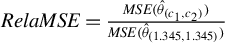 $RelaMSE=\frac {MSE(\hat {\theta }_{(c_{1},c_{2})})}{MSE(\hat {\theta }_{(1.345,1.345)})}$
. The results regarding
$RelaMSE=\frac {MSE(\hat {\theta }_{(c_{1},c_{2})})}{MSE(\hat {\theta }_{(1.345,1.345)})}$
. The results regarding
 $\lambda $
and
$\lambda $
and
 $\beta _{2}$
are presented in Tables E.2 and E.3 in the Supplementary Material. In general, the relative MSEs of both
$\beta _{2}$
are presented in Tables E.2 and E.3 in the Supplementary Material. In general, the relative MSEs of both
 $\hat {\lambda }$
and
$\hat {\lambda }$
and
 $\hat {\beta }_{2}$
tend to get larger when
$\hat {\beta }_{2}$
tend to get larger when
 $c_{2}\geq 1.8$
and do not vary much for
$c_{2}\geq 1.8$
and do not vary much for
 $c_{2}\in [1,1.5]$
. For a fixed
$c_{2}\in [1,1.5]$
. For a fixed
 $c_{2}$
, especially when
$c_{2}$
, especially when
 $c_{2}\in [1,1.5]$
, the influence of
$c_{2}\in [1,1.5]$
, the influence of
 $c_{1}$
on the relative MSE is rather small, with variations typically within 5% in most cases. In cases where there is no clear pattern, such as the relative RMSE of
$c_{1}$
on the relative MSE is rather small, with variations typically within 5% in most cases. In cases where there is no clear pattern, such as the relative RMSE of
 $\hat {\lambda }$
in scenario (2),
$\hat {\lambda }$
in scenario (2),
 $(c_{1},c_{2})=(1.345,1.345)$
dominates most other tuning parameter combinations. Thus, Eq. (2.7) serves as a reasonable criterion for selecting M with
$(c_{1},c_{2})=(1.345,1.345)$
dominates most other tuning parameter combinations. Thus, Eq. (2.7) serves as a reasonable criterion for selecting M with
 $(c_{1},c_{2})=(1.345,1.345)$
, and there is no need to differentiate
$(c_{1},c_{2})=(1.345,1.345)$
, and there is no need to differentiate
 $c_{1}$
and
$c_{1}$
and
 $c_{2}$
.
$c_{2}$
.
In conclusion, for both the HIV estimator and the HGMM estimator, our simulation results indicate that
 $c=1.345$
is a satisfactory choice for a variety of scenarios, including contaminated data, long-tailed data, and data with conditional heteroskedasticity. Thus, we maintain
$c=1.345$
is a satisfactory choice for a variety of scenarios, including contaminated data, long-tailed data, and data with conditional heteroskedasticity. Thus, we maintain
 $c=1.345$
in our subsequent simulation studies.
$c=1.345$
in our subsequent simulation studies.
4.2 Compare the Performance of Various Estimators
Next, we compare the performances of the QMLE, the 2SLS estimator in Kelejian and Prucha (Reference Kelejian and Prucha1998), the BIV estimator in Lee (Reference Lee2003), the GMM estimators in Lin and Lee (Reference Lin and Lee2010), the quantile IV (QIV) estimator in Su and Yang (Reference Su and Yang2011), the 2SGM estimator in Wagenvoort and Waldmann (Reference Wagenvoort and Waldmann2002),Footnote
16
the Huber maximum likelihood estimator (HMLE) in Tho et al. (Reference Tho, Ding, Hui, Welsh and Zou2023), and the three estimators proposed in our article: the HIV estimator, the BHIV estimator, and HGMM estimator. For both the GMM estimator and the HGMM estimator, we adopt
 $P_{n}=\tilde {G}_{n}-\operatorname {\mathrm {diag}}(\tilde {G}_{n})$
for the quadratic moments, where
$P_{n}=\tilde {G}_{n}-\operatorname {\mathrm {diag}}(\tilde {G}_{n})$
for the quadratic moments, where
 $\tilde {G}_{n}=W_{n}(I_{n}-\tilde {\lambda }W_{n})^{-1}$
, and
$\tilde {G}_{n}=W_{n}(I_{n}-\tilde {\lambda }W_{n})^{-1}$
, and
 $\tilde {\lambda }$
is a consistent estimator for
$\tilde {\lambda }$
is a consistent estimator for
 $\lambda _{0}$
.Footnote
17
And we use
$\lambda _{0}$
.Footnote
17
And we use
 $X_{n}$
and
$X_{n}$
and
 $G_{n}X_{n}\tilde {\beta }$
as the IVs, where
$G_{n}X_{n}\tilde {\beta }$
as the IVs, where
 $\tilde {\beta }$
is a consistent estimator for the true parameter value
$\tilde {\beta }$
is a consistent estimator for the true parameter value
 $\beta _{0}$
. For Huber type estimators, the critical value of M is determined as in Section 2.3 with
$\beta _{0}$
. For Huber type estimators, the critical value of M is determined as in Section 2.3 with
 $c=1.345$
.
$c=1.345$
.
We have tried three different sample sizes in the experiments:
 $n=100,200,$
and 400. For each setting, simulations are repeated 1,000 times to obtain these estimates’ sample bias and RMSE. We report the results on parameters
$n=100,200,$
and 400. For each setting, simulations are repeated 1,000 times to obtain these estimates’ sample bias and RMSE. We report the results on parameters
 $\lambda $
and
$\lambda $
and
 $\beta _{2}$
under sample sizes
$\beta _{2}$
under sample sizes
 $n=100$
and
$n=100$
and
 $n=400$
in Tables 1 and 2, respectively. Full results—including all parameters (except for the intercept coefficient
$n=400$
in Tables 1 and 2, respectively. Full results—including all parameters (except for the intercept coefficient
 $\beta _{1}$
) and all sample sizes (
$\beta _{1}$
) and all sample sizes (
 $n=100, 200, 400$
)—are provided in Tables E.4–E.6 in the Supplementary Material. Under asymmetrically distributed disturbances, the true intercept
$n=100, 200, 400$
)—are provided in Tables E.4–E.6 in the Supplementary Material. Under asymmetrically distributed disturbances, the true intercept
 $\beta _{10}$
depends on the critical value M, and is different from the true intercept under the moment condition
$\beta _{10}$
depends on the critical value M, and is different from the true intercept under the moment condition
 $\operatorname {\mathrm {E}}\epsilon _{i,n}=0$
, so it is troublesome to compare its estimates. Thus, we omit them from all reported tables—including the full results in Tables E.4–E.6 in the Supplementary Material. To obtain a better insight into the merits of robust estimators, we present the relative efficiency of each Huber-type estimator
$\operatorname {\mathrm {E}}\epsilon _{i,n}=0$
, so it is troublesome to compare its estimates. Thus, we omit them from all reported tables—including the full results in Tables E.4–E.6 in the Supplementary Material. To obtain a better insight into the merits of robust estimators, we present the relative efficiency of each Huber-type estimator
 $\hat {\theta }$
compared to its corresponding traditional estimator, e.g., HIV/2SLS, BHIV/BIV, and HGMM/GMM, in Table 3. The relative efficiency of
$\hat {\theta }$
compared to its corresponding traditional estimator, e.g., HIV/2SLS, BHIV/BIV, and HGMM/GMM, in Table 3. The relative efficiency of
 $\hat {\theta }_{1}$
relative to
$\hat {\theta }_{1}$
relative to
 $\hat {\theta }_{2}$
is calculated as
$\hat {\theta }_{2}$
is calculated as
 $MSE(\hat {\theta }_{2})/MSE(\hat {\theta }_{1})$
.
$MSE(\hat {\theta }_{2})/MSE(\hat {\theta }_{1})$
.
Estimation results (
 $n=100$
)
$n=100$
)

1: iid
 $N(0,1)$
; 2: Mixed normal: iid
$N(0,1)$
; 2: Mixed normal: iid
 $0.95N(0,1)+0.05N(0,25)$
; 3: NC:
$0.95N(0,1)+0.05N(0,25)$
; 3: NC:
 $0.95N(0,1)+0.05t_{1}$
; 4: Extreme contamination:
$0.95N(0,1)+0.05t_{1}$
; 4: Extreme contamination:
 $\epsilon _{1}\sim N(150,1)$
; 5: Extreme contamination:
$\epsilon _{1}\sim N(150,1)$
; 5: Extreme contamination:
 $\epsilon _{1},\epsilon _{2}\sim N(150,1)$
; 6: Laplace
$\epsilon _{1},\epsilon _{2}\sim N(150,1)$
; 6: Laplace
 $\cdot x_{i2,n}$
: Laplace distribution scaled by
$\cdot x_{i2,n}$
: Laplace distribution scaled by
 $x_{i2}$
; and 7:
$x_{i2}$
; and 7:
 $\exp (1)\cdot x_{i2,n}^{2}$
:
$\exp (1)\cdot x_{i2,n}^{2}$
:
 $\exp (1)$
scaled by
$\exp (1)$
scaled by
 $x_{i2,n}^{2}$
. BIV: Best IV; GMM: GMM in Lin and Lee (Reference Lin and Lee2010); QIV: quantile IV in Su and Yang (Reference Su and Yang2011); 2SGM: Two-stage generalized M-estimator in Wagenvoort and Waldmann (Reference Wagenvoort and Waldmann2002); HMLE: Huber MLE in Tho et al. (Reference Tho, Ding, Hui, Welsh and Zou2023); HIV: Huber IV; BHIV: Best Huber IV; and HGMM: Huber GMM.
$x_{i2,n}^{2}$
. BIV: Best IV; GMM: GMM in Lin and Lee (Reference Lin and Lee2010); QIV: quantile IV in Su and Yang (Reference Su and Yang2011); 2SGM: Two-stage generalized M-estimator in Wagenvoort and Waldmann (Reference Wagenvoort and Waldmann2002); HMLE: Huber MLE in Tho et al. (Reference Tho, Ding, Hui, Welsh and Zou2023); HIV: Huber IV; BHIV: Best Huber IV; and HGMM: Huber GMM.
Estimation results (
 $n=400$
)
$n=400$
)

1: iid
 $N(0,1)$
; 2: Mixed normal: iid
$N(0,1)$
; 2: Mixed normal: iid
 $0.95N(0,1)+0.05N(0,25)$
; 3: NC:
$0.95N(0,1)+0.05N(0,25)$
; 3: NC:
 $0.95N(0,1)+0.05t_{1}$
; 4: Extreme contamination:
$0.95N(0,1)+0.05t_{1}$
; 4: Extreme contamination:
 $\epsilon _{1}\sim N(150,1)$
; 5: Extreme contamination:
$\epsilon _{1}\sim N(150,1)$
; 5: Extreme contamination:
 $\epsilon _{1},\epsilon _{2}\sim N(150,1)$
; 6: Laplace
$\epsilon _{1},\epsilon _{2}\sim N(150,1)$
; 6: Laplace
 $\cdot x_{i2,n}$
: Laplace distribution scaled by
$\cdot x_{i2,n}$
: Laplace distribution scaled by
 $x_{i2}$
; and 7:
$x_{i2}$
; and 7:
 $\exp (1)\cdot x_{i2,n}^{2}$
:
$\exp (1)\cdot x_{i2,n}^{2}$
:
 $\exp (1)$
scaled by
$\exp (1)$
scaled by
 $x_{i2,n}^{2}$
. BIV: Best IV; GMM: GMM in Lin and Lee (Reference Lin and Lee2010); QIV: quantile IV in Su and Yang (Reference Su and Yang2011); 2SGM: Two-stage generalized M-estimator in Wagenvoort and Waldmann (Reference Wagenvoort and Waldmann2002); HMLE: Huber MLE in Tho et al. (Reference Tho, Ding, Hui, Welsh and Zou2023); HIV: Huber IV; BHIV: Best Huber IV; and HGMM: Huber GMM.
$x_{i2,n}^{2}$
. BIV: Best IV; GMM: GMM in Lin and Lee (Reference Lin and Lee2010); QIV: quantile IV in Su and Yang (Reference Su and Yang2011); 2SGM: Two-stage generalized M-estimator in Wagenvoort and Waldmann (Reference Wagenvoort and Waldmann2002); HMLE: Huber MLE in Tho et al. (Reference Tho, Ding, Hui, Welsh and Zou2023); HIV: Huber IV; BHIV: Best Huber IV; and HGMM: Huber GMM.
Relative efficiency of Huber estimators with respect to traditional estimators

1: iid
 $N(0,1)$
; 2: Mixed normal: iid
$N(0,1)$
; 2: Mixed normal: iid
 $0.95N(0,1)+0.05N(0,25)$
; 3: NC: iid
$0.95N(0,1)+0.05N(0,25)$
; 3: NC: iid
 $0.95N(0,1)+0.05t_{1}$
; 4: Extreme contamination:
$0.95N(0,1)+0.05t_{1}$
; 4: Extreme contamination:
 $\epsilon _{1}\sim N(150,1)$
; 5: Extreme contamination:
$\epsilon _{1}\sim N(150,1)$
; 5: Extreme contamination:
 $\epsilon _{1},\epsilon _{2}\sim N(150,1)$
; 6: Laplace
$\epsilon _{1},\epsilon _{2}\sim N(150,1)$
; 6: Laplace
 $\cdot x_{i2,n}$
: Laplace distribution scaled by
$\cdot x_{i2,n}$
: Laplace distribution scaled by
 $x_{i2}$
; and 7:
$x_{i2}$
; and 7:
 $\exp (1)\cdot x_{i2,n}^{2}$
:
$\exp (1)\cdot x_{i2,n}^{2}$
:
 $\exp (1)$
scaled by
$\exp (1)$
scaled by
 $x_{i2,n}^{2}$
. BIV: Best IV; GMM: GMM in Lin and Lee (Reference Lin and Lee2010): HIV: Huber IV; BHIV: Best Huber IV; HGMM: Huber GMM. Relative efficiency=
$x_{i2,n}^{2}$
. BIV: Best IV; GMM: GMM in Lin and Lee (Reference Lin and Lee2010): HIV: Huber IV; BHIV: Best Huber IV; HGMM: Huber GMM. Relative efficiency=
 $MSE(\hat {\theta }_{traditional})/MSE(\hat {\theta }_{Huber})$
.
$MSE(\hat {\theta }_{traditional})/MSE(\hat {\theta }_{Huber})$
.
Below are some interesting observations obtained from the simulation results:
(1) For all sample sizes and distributions, the biases and RMSEs of the three proposed Huber estimators are notably small. As the sample size n increases, the RMSEs of our estimators decrease at roughly the rate of
 $n^{-1/2}$
. For instance, under the mixed normal distribution, when
$n^{-1/2}$
. For instance, under the mixed normal distribution, when
 $n=100$
, 200, and 400, the RMSE for
$n=100$
, 200, and 400, the RMSE for
 $\hat {\lambda }_{HGMM}$
is 0.0661, 0.0473, and 0.0378, respectively. These results conform with the prediction of our large sample theories.
$\hat {\lambda }_{HGMM}$
is 0.0661, 0.0473, and 0.0378, respectively. These results conform with the prediction of our large sample theories.
(2) When the disturbances are i.i.d. normally distributed,
 $$\begin{align*}QMLE &\succsim GMM\succsim HGMM\succsim HMLE\succ2SLS\approx BIV\\ & \approx HIV\approx BHIV\succ2SGM\succ QIV, \end{align*}$$
where
 $\succ $
means “performing better than,”
$\succ $
means “performing better than,”
 $\succsim $
means “performing slightly better than,” and
$\succsim $
means “performing slightly better than,” and
 $\approx $
means “performing similarly.” Although QMLE performs the best, the differences between the HGMM estimator, the GMM estimator, and the QMLE are minor. Among all robust estimators, the HGMM estimator exhibits the smallest efficiency loss under
$\approx $
means “performing similarly.” Although QMLE performs the best, the differences between the HGMM estimator, the GMM estimator, and the QMLE are minor. Among all robust estimators, the HGMM estimator exhibits the smallest efficiency loss under
 $N(0,1)$
. For all sample sizes and all parameters,
$N(0,1)$
. For all sample sizes and all parameters,
 $$\begin{align*}\frac{RMSE(HGMM)-RMSE(QMLE)}{RMSE(QMLE)}<2\%, \end{align*}$$
 $$\begin{align*}\frac{RMSE(HGMM)-RMSE(GMM)}{RMSE(GMM)}<2\%. \end{align*}$$
From Table 3, under normally distributed disturbances, Huber-type estimators exhibit only a slight loss in efficiency (in most cases
 $<6\%$
) compared to traditional estimators. This modest efficiency trade-off is to be expected, as robustness often comes at the cost of some efficiency. The efficiency losses incurred by our estimators are minimal. The aforementioned observations can be clearly seen from Figures 1 and 2. Please note that each pair of bars sharing similar colors in the figure represents a traditional estimator and its Huber variant, respectively (for instance, 2SLS and HIV, BIV and BHIV, and GMM and HGMM estimators), while the purple bars represent 2SGM estimator and QIV estimator.
$<6\%$
) compared to traditional estimators. This modest efficiency trade-off is to be expected, as robustness often comes at the cost of some efficiency. The efficiency losses incurred by our estimators are minimal. The aforementioned observations can be clearly seen from Figures 1 and 2. Please note that each pair of bars sharing similar colors in the figure represents a traditional estimator and its Huber variant, respectively (for instance, 2SLS and HIV, BIV and BHIV, and GMM and HGMM estimators), while the purple bars represent 2SGM estimator and QIV estimator.
RMSE of
 $\hat {\lambda }$
of various estimators under
$\hat {\lambda }$
of various estimators under
 $N(0,1)$
.
$N(0,1)$
.

RMSE of
 $\hat {\beta }_{2}$
of various estimators under
$\hat {\beta }_{2}$
of various estimators under
 $N(0,1)$
.
$N(0,1)$
.

(3) In extreme contamination scenarios (cases 4 and 5), the biases and RMSEs of the traditional estimators, including QMLE, 2SLS, BIV, and GMM, are extremely large, among which BIV is the worst (when
 $n=100$
, for
$n=100$
, for
 $\lambda $
, the efficiency of the BHIV estimator compared to the BIV estimator is
$\lambda $
, the efficiency of the BHIV estimator compared to the BIV estimator is
 $3.2\times 10^{5}$
). In contrast, all robust estimators exhibit significantly superior performance. The Huber MLE is slightly better than HGMM, but the difference is minimal. Both significantly outperform other robust estimators. Overall, we summarize performances of these estimators in most (although not all) cases as follows:
$3.2\times 10^{5}$
). In contrast, all robust estimators exhibit significantly superior performance. The Huber MLE is slightly better than HGMM, but the difference is minimal. Both significantly outperform other robust estimators. Overall, we summarize performances of these estimators in most (although not all) cases as follows:
 $$\begin{align*}HMLE &\succsim HGMM\succ BHIV\succ HIV\succ QIV\succ2SGM\succ QMLE\\ &\succ2SLS\approx GMM\succ BIV. \end{align*}$$
The conclusions for setups (2) and (3) are similar.
(4) In the presence of conditional heteroskedasticity (cases 6 and 7), the HGMM estimator and QIV estimator outperform other robust estimators, which in turn perform better than traditional estimators. We can see this more clearly from Figures 3 and 4. Results can be summarized as follows:
 $$\begin{align*}HGMM &\approx QIV\succ BHIV\succ HIV\approx HMLE\succ2SGM\succ GMM\\ & \approx QMLE\succ2SLS\succ BIV. \end{align*}$$
RMSE of
 $\hat {\lambda }$
of various estimators under
$\hat {\lambda }$
of various estimators under
 $Laplace\cdot x_{i2}$
.
$Laplace\cdot x_{i2}$
.

RMSE of
 $\hat {\beta }_{2}$
of various estimators under
$\hat {\beta }_{2}$
of various estimators under
 $Laplace\cdot x_{i2}$
.
$Laplace\cdot x_{i2}$
.

(5) In all setups (2)–(7), which involve contaminated, long-tailed, or conditionally heteroskedastic disturbances, Huber-type estimators consistently outperform their traditional counterparts:
 $$\begin{align*}\begin{cases} \begin{array}{@{}cc} HGMM\succ GMM, & \\ BHIV\succ BIV, & \\ HIV\succ2SLS. & \end{array}\end{cases} \end{align*}$$
(6) All the proposed estimators are computationally efficient. For example, when the errors follow a mixed normal distribution and the sample size
 $n=100$
, our desktop computer (CPU: Intel(R) Xeon(R) E-2136; RAM: 32G; hard drive: 1T; and software: MATLAB) takes an average of 0.013 seconds to run the HGMM estimation and 0.25 seconds for the Huber MLE by Tho et al. (Reference Tho, Ding, Hui, Welsh and Zou2023). With
$n=100$
, our desktop computer (CPU: Intel(R) Xeon(R) E-2136; RAM: 32G; hard drive: 1T; and software: MATLAB) takes an average of 0.013 seconds to run the HGMM estimation and 0.25 seconds for the Huber MLE by Tho et al. (Reference Tho, Ding, Hui, Welsh and Zou2023). With
 $n=400$
, the HGMM estimation takes 0.047 seconds, while the Huber MLE takes 5 seconds. On average, our estimators can be computed 20 times faster than the estimator in Tho et al. (Reference Tho, Ding, Hui, Welsh and Zou2023) for
$n=400$
, the HGMM estimation takes 0.047 seconds, while the Huber MLE takes 5 seconds. On average, our estimators can be computed 20 times faster than the estimator in Tho et al. (Reference Tho, Ding, Hui, Welsh and Zou2023) for
 $n=100$
, and 100 times faster for
$n=100$
, and 100 times faster for
 $n=400$
.
$n=400$
.
In conclusion, the simulation outcomes demonstrate that our estimators are robust against both contaminated or long-tailed disturbances and conditional heteroskedasticity, incur minimal efficiency loss under short-tailed disturbances, and are computationally convenient. The Huber MLE by Tho et al. (Reference Tho, Ding, Hui, Welsh and Zou2023) works well under contaminated disturbances, but is less robust to conditional heteroskedasticity, and computationally slower. QIV estimator excels under heteroskedastic long-tailed disturbances, but performs worse than the HGMM estimator and the Huber MLE in other scenarios. Overall, HGMM estimator performs the best among all these estimators in simulations.
4.3 A Test Experiment
We further carry out simulation studies to evaluate the empirical size and the power of testing
 $H_{0}:\beta _{20}=\beta _{30}$
vs.
$H_{0}:\beta _{20}=\beta _{30}$
vs.
 $H_{0}:\beta _{20}\neq {{\beta _{30}}}$
at level 5%, as suggested by an anonymous referee. The experimental setup closely follows that of Section 4.3, except that
$H_{0}:\beta _{20}\neq {{\beta _{30}}}$
at level 5%, as suggested by an anonymous referee. The experimental setup closely follows that of Section 4.3, except that
 $\beta _{30}\in \{1,-1\}$
. Detailed results are reported in Tables E.7 and E.8 in the Supplementary Material. We observe that the empirical size is around 0.05 and the empirical power is close to 1 for all settings and all sample sizes. As the sample size increases, the empirical size gets closer to 0.05 and the empirical power tends toward 1. This shows that our asymptotic distribution approximates the true distribution of the estimators well.
$\beta _{30}\in \{1,-1\}$
. Detailed results are reported in Tables E.7 and E.8 in the Supplementary Material. We observe that the empirical size is around 0.05 and the empirical power is close to 1 for all settings and all sample sizes. As the sample size increases, the empirical size gets closer to 0.05 and the empirical power tends toward 1. This shows that our asymptotic distribution approximates the true distribution of the estimators well.
5 EFFECT OF URBAN HEAT ISLAND ON HOUSING PRICES
From the Monte Carlo study, it is evident that the HGMM estimation significantly outperforms in scenarios characterized by long-tailed disturbances and conditional heteroskedasticity. In this section, we employ the HGMM approach to identify the effect of urban heat island on surrounding housing prices in Beijing of China, using the data in 2017 from Lin et al. (Reference Lin, Meng, Mei, Zhang, Liu and Xiang2022). In our analysis, each individual is a community, the explained variable is the logarithm of the average housing prices in a community, and the variable of interest is an index of urban heat island intensity (UHII).
The urban heat island effect refers to a phenomenon in which the temperature in urban areas is higher than that in the surrounding countryside (Mohajerani, Bakaric, and Jeffrey-Bailey, Reference Mohajerani, Bakaric and Jeffrey-Bailey2017). Due to the high temperature near the ground in the central area of the heat island, the atmosphere moves upward, forming a pressure difference with the surrounding areas. The near-ground atmosphere in the surrounding areas converges to the central area, forming a low-pressure vortex in the central area of the city, resulting in the accumulation of sulfur oxides, nitrogen oxides, carbon oxides, hydrocarbons, and other air pollutants formed by burning fossil fuels in people’s lives, industrial production, and vehicle operation in the central area of the heat island (Zhong et al., Reference Zhong, Qian, Zhao, Leung, Wang, Yang, Fan, Yan, Yang and Liu2017). The warming effect of urbanization is believed to pose a major risk to public health, such as emotional irritability, mental depression, insomnia, anorexia, dyspepsia, increased ulcers, recurrence of gastrointestinal diseases, etc. (Hsu et al., Reference Hsu, Sheriff, Chakraborty and Manya2021). The urban heat island effect in high-temperature weather also increases the possibility for residents to use air conditioners, electric fans, and other electrical appliances, thus bolstering electricity consumption, increasing the power load, and generating more waste heat to further enhance the heat island effect. Due to its critical impact on human health and comfort, the urban heat island effect can be capitalized into housing prices by affecting residents’ choices in home purchasing.
Plantinga et al. (Reference Plantinga, Détang-Dessendre, Hunt and Piguet2013) find that residents prefer higher January temperatures but dislike higher July temperatures. Klaiber, Abbott, and Smith (Reference Klaiber, Abbott and Smith2017) hold that homeowners value cooler temperatures. Lin et al. (Reference Lin, Meng, Mei, Zhang, Liu and Xiang2022) establish an index for UHII by using temperature difference between impervious surfaces and other types of land use to measure urban heat island effect. They find a similar result: a one-unit increase in the UHII is associated with a 3.91% decrease in home values in Beijing, China. However, their estimation procedure does not address the issue of long-tailed feature and conditional heteroskedasticity of housing price data and may result in larger standard errors if that is the case. To accommodate this issue, we adopt the HGMM approach proposed in this article to examine the urban heat island effect on housing prices in Beijing.
The variable of interest is the UHII proposed by Lin et al. (Reference Lin, Meng, Mei, Zhang, Liu and Xiang2022). Control variables include whether a community is located in a top ten primary school district, housing age, distance to the nearest park and subway, normalized difference built-up index (NDBI), and normalized difference vegetation index (NDVI). The detailed definitions and summary statistics are detailed in Table 4. Because housing prices are spatially correlated in nature (Irwin, Jeanty, and Partridge, Reference Irwin, Jeanty and Partridge2014), we employ an SAR model to control for spatial correlation among housing prices. For the spatial weights matrix
 $W_{n}\equiv (w_{ij})_{n\times n}$
,
$W_{n}\equiv (w_{ij})_{n\times n}$
,
 $w_{ij}=\frac {1}{4}$
if j is among the four nearest neighbors of i,
$w_{ij}=\frac {1}{4}$
if j is among the four nearest neighbors of i,
 $w_{ij}=0$
otherwise. The estimation results are summarized in Table 5. To ascertain the robustness of our estimation findings, we explore two alternative specifications for the spatial weights matrix: (1)
$w_{ij}=0$
otherwise. The estimation results are summarized in Table 5. To ascertain the robustness of our estimation findings, we explore two alternative specifications for the spatial weights matrix: (1)
 $w_{ij}=1/6$
if j is among the six nearest neighbors of i, and
$w_{ij}=1/6$
if j is among the six nearest neighbors of i, and
 $w_{ij}=0$
otherwise and (2)
$w_{ij}=0$
otherwise and (2)
 $w_{ij}\propto d_{ij}^{-5}$
with the spatial weights matrix row normalized. In the second case, the spatial weights are a decreasing function of distances between communities. These additional estimation results are summarized in Tables F.1 and F.2 in the Supplementary Material.
$w_{ij}\propto d_{ij}^{-5}$
with the spatial weights matrix row normalized. In the second case, the spatial weights are a decreasing function of distances between communities. These additional estimation results are summarized in Tables F.1 and F.2 in the Supplementary Material.
Definitions and statistical summary of UHI data

Estimation results under
 $W_{4n}$

 $**$
and
$**$
and
 $***$
: Significant at levels 5% and 1%. Standard deviation: Heteroskedasticity-consistent estimator.
$***$
: Significant at levels 5% and 1%. Standard deviation: Heteroskedasticity-consistent estimator.
To demonstrate the importance of the HGMM approach, we compare it with two traditional estimation methods for the SAR model: QMLE and the traditional GMM approach in Lin and Lee (Reference Lin and Lee2010). We also perform a naive OLS estimation. From Table 5 and Tables F.1 and F.2 in the Supplementary Material, we observe both conditional heteroskedasticity and a long-tailed distribution in the error terms:
-
1. There exists conditional heteroskedasticity. For every method, we regress
 $\hat {\epsilon }_{i,n}^{2}$
on
$x_{i,n}$
, where
$\hat {\epsilon }_{i,n}$
is the residual, and calculate the test statistic
$nR^{2}$
to test whether there exists conditional heteroskedasticity. And the test statistics are always greater than
$370$
, and the corresponding p-values are 0. So, there is convincing evidence that there exists conditional heteroskedasticity.
$\hat {\epsilon }_{i,n}^{2}$
on
$x_{i,n}$
, where
$\hat {\epsilon }_{i,n}$
is the residual, and calculate the test statistic
$nR^{2}$
to test whether there exists conditional heteroskedasticity. And the test statistics are always greater than
$370$
, and the corresponding p-values are 0. So, there is convincing evidence that there exists conditional heteroskedasticity. -
2. The error terms follow a long-tailed distribution. In most results, the residuals exhibit a kurtosis of approximately 9; in one case, it is 69.9. So, the kurtosis of the residuals is clearly greater than 3 (the kurtosis of the normal distribution), which indicates that the disturbances are long-tailed or there exist outliers.


Given the above observations, because both the QMLE and the Huber MLE for the SAR model assume i.i.d. errors and the GMM estimator in Lin and Lee (Reference Lin and Lee2010) is sensitive to long-tailed distributions as indicated by simulation studies, the HGMM estimation is suitable for this dataset. As in Section 4, we set
 ${P_{n}=\tilde {G}_{n}-\operatorname {\mathrm {diag}}(\tilde {G}_{n})}$
, where
${P_{n}=\tilde {G}_{n}-\operatorname {\mathrm {diag}}(\tilde {G}_{n})}$
, where
 $\tilde {G}_{n}=W_{n}(I_{n}-\tilde {\lambda }W_{n})^{-1}$
and
$\tilde {G}_{n}=W_{n}(I_{n}-\tilde {\lambda }W_{n})^{-1}$
and
 $\tilde {\lambda }$
is a consistent estimator for
$\tilde {\lambda }$
is a consistent estimator for
 $\lambda _{0}$
.Footnote
18
The corresponding estimators are denoted as GMM and HGMM, respectively. The value of M is determined as in Section 2.3. From Table 5, the estimates of the spatial interaction coefficient
$\lambda _{0}$
.Footnote
18
The corresponding estimators are denoted as GMM and HGMM, respectively. The value of M is determined as in Section 2.3. From Table 5, the estimates of the spatial interaction coefficient
 $\lambda $
in columns 2–4 are all significant and range between 0.5 and 0.63, indicating a strong spatial correlation in housing prices. The absolute values of the naive OLS coefficients are bigger than other estimates in general. So, the effects of UHII and the control variables are probably overestimated if we ignore the spatial correlation in housing prices. Moreover, the standard errors of all the estimates from HGMM are smaller than those of GMM, indicating our HGMM approach is more robust and precise than traditional GMM estimators for this dataset. For UHII in the SAR model, all estimation methods yield significant estimates at the 1% level, showing that higher UHII leads to lower housing prices. The QMLE and the traditional GMM estimates are both
$\lambda $
in columns 2–4 are all significant and range between 0.5 and 0.63, indicating a strong spatial correlation in housing prices. The absolute values of the naive OLS coefficients are bigger than other estimates in general. So, the effects of UHII and the control variables are probably overestimated if we ignore the spatial correlation in housing prices. Moreover, the standard errors of all the estimates from HGMM are smaller than those of GMM, indicating our HGMM approach is more robust and precise than traditional GMM estimators for this dataset. For UHII in the SAR model, all estimation methods yield significant estimates at the 1% level, showing that higher UHII leads to lower housing prices. The QMLE and the traditional GMM estimates are both
 $-$
0.0116, while the HGMM estimate is
$-$
0.0116, while the HGMM estimate is
 $-$
0.0082. It seems that QMLE and the traditional GMM tend to overestimate the effects of the urban heat island.
$-$
0.0082. It seems that QMLE and the traditional GMM tend to overestimate the effects of the urban heat island.
When considering the six nearest neighbors setting for
 $W_{n}$
, the estimation results (Table F.1 in the Supplementary Material) are similar. However, when considering the setting
$W_{n}$
, the estimation results (Table F.1 in the Supplementary Material) are similar. However, when considering the setting
 $w_{ij}\propto d_{ij}^{-5}$
for
$w_{ij}\propto d_{ij}^{-5}$
for
 $W_{n}$
, from Table F.2 in the Supplementary Material, compared to the HGMM estimation, the traditional GMM estimation drastically underestimates the spatial interaction coefficient. It suggests that the first two setups for
$W_{n}$
, from Table F.2 in the Supplementary Material, compared to the HGMM estimation, the traditional GMM estimation drastically underestimates the spatial interaction coefficient. It suggests that the first two setups for
 $W_{n}$
are more reliable.
$W_{n}$
are more reliable.
6 CONCLUSION
In this article, we introduce two computationally convenient estimators for the SAR model that are robust to both long-tailed disturbances and conditional heteroskedasticity: the HIV estimator and the HGMM estimator. Unlike the Huber MLE proposed by Tho et al. (Reference Tho, Ding, Hui, Welsh and Zou2023), our estimators are also robust to conditional heteroskedasticity. They are not only robust to long-tailed disturbances but also incur minimal efficiency loss compared to traditional estimators for the SAR model under short-tailed disturbances. We establish their large sample properties by extending the empirical process results on non-differentiable objective functions in Pollard (Reference Pollard1985)to allow heterogeneous and mutually correlated data. We show that our estimators are consistent under regularity conditions, even when the expectation of the error terms does not exist. In addition, we discuss the breakdown point of our estimators and show that the influence functions of our estimators are bounded. We also extend our estimation methods to the SARARE model, whose error terms are spatially correlated. Simulation studies confirm that these estimators outperform the corresponding traditional estimators when error terms are long-tailed or there exist outliers. Finally, we apply the HGMM estimation to study the effect of urban heat island on housing prices in Beijing. Given the conditional heteroskedasticity and the long-tailed distribution of the error terms, the HGMM estimation is well-suited for this dataset. Our study provides more reliable evidence that the urban heat island effects contribute to a reduction in housing prices in big cities.
We have made our MATLAB code publicly available to support replication and further empirical applications. The code is accessible at: https://github.com/Xingbai2004/Huber-GMM.
SUPPLEMENTARY MATERIAL
Liu, T., Xu, X., Lee, L.-F., & Mei, Y. (2026). Supplement to “Robust estimation for the spatial autoregressive model,” Econometric Theory Supplementary Material. To view, please visit: https://doi.org/10.1017/S0266466626100346.
FUNDING STATEMENT
T.L. gratefully acknowledges the financial support of the Chinese National Natural Science Fund of China (CNNSF) (Grant Nos. 71903163 and 72033008). X.X. gratefully acknowledges the financial support of the CNNSF (Grant Nos. 72073110, 72473118, and 72333001), Basic Scientific Center Project 71988101 of CNNSF, and the 111 Project (B13028). L.-F.L. gratefully acknowledges the financial support of CNNSF (Grant No. 72333002).
COMPETING INTEREST STATEMENT
The authors declare that no competing interests exist.
Appendixes
A SOME LEMMAS
The proofs of the following lemmas are collected in Section D of the Supplementary Material.
Lemma A.1. Suppose that
 $\operatorname {\mathrm {E}}|X|^{\gamma }<\infty $
for some constant
$\operatorname {\mathrm {E}}|X|^{\gamma }<\infty $
for some constant
 $\gamma>0$
and
$\gamma>0$
and
 $M>0$
is a constant. Let
$M>0$
is a constant. Let
 $p\ge \max (1,\gamma )$
be a constant. Then,
$p\ge \max (1,\gamma )$
be a constant. Then,
 $$\begin{align*}\left\Vert \min(M,|X|)\right\Vert _{L^{p}}\leq M^{1-\gamma/p}\left(\operatorname{\mathrm{E}}|X|^{\gamma}\right)^{1/p}. \end{align*}$$
Lemma A.2.
 $\gamma \in [1,2)$
is a constant. Suppose that
$\gamma \in [1,2)$
is a constant. Suppose that
 $\{v_{i,n}:i\in D_{n}\}_{n\in \mathbb {N}}$
is uniformly
$\{v_{i,n}:i\in D_{n}\}_{n\in \mathbb {N}}$
is uniformly
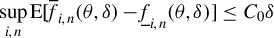 $L_{\gamma }$
-NED on
$L_{\gamma }$
-NED on
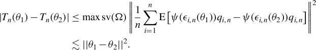 $\{\epsilon _{i,n}:i\in D_{n}\}_{n\in \mathbb {N}}$
:
$\{\epsilon _{i,n}:i\in D_{n}\}_{n\in \mathbb {N}}$
:
 $||v_{i,n}-\operatorname {\mathrm {E}}[v_{i,n}|\mathcal {F}_{i,n}(s)]||_{L^{\gamma }}\leq \psi (s)$
for all i, n, and some non-increasing function
$||v_{i,n}-\operatorname {\mathrm {E}}[v_{i,n}|\mathcal {F}_{i,n}(s)]||_{L^{\gamma }}\leq \psi (s)$
for all i, n, and some non-increasing function
 $\psi (\cdot )$
satisfying
$\psi (\cdot )$
satisfying
 $\lim _{s\to \infty }\psi (s)=0$
, where
$\lim _{s\to \infty }\psi (s)=0$
, where
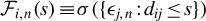 ${\mathcal {F}_{i,n}(s){\kern-1pt}\equiv{\kern-1pt} \sigma (\{\epsilon _{j,n}{\kern-1pt}:{\kern-1pt}d_{ij}{\kern-1pt}\leq{\kern-1pt} s\})}$
is the sub-
${\mathcal {F}_{i,n}(s){\kern-1pt}\equiv{\kern-1pt} \sigma (\{\epsilon _{j,n}{\kern-1pt}:{\kern-1pt}d_{ij}{\kern-1pt}\leq{\kern-1pt} s\})}$
is the sub-
 $\sigma $
-field generated by those
$\sigma $
-field generated by those
 $\epsilon _{j,n}$
’s with
$\epsilon _{j,n}$
’s with
 $d_{ij}\leq s$
.
$d_{ij}\leq s$
.
 $F(\cdot )$
is an
$F(\cdot )$
is an
 $\mathbb {R}$
-valued function bounded by a constant M and is a Lipschitz function with a Lipschitz constant L. Then,
$\mathbb {R}$
-valued function bounded by a constant M and is a Lipschitz function with a Lipschitz constant L. Then,
 $\|F(v_{i,n})-\operatorname {\mathrm {E}}[v_{i,n}|\mathcal {F}_{i,n}(s)]||_{L^{2}}\leq (2M)^{1-\gamma /2}L^{\gamma /2}\psi (s)^{\gamma /2}$
for all i and n.
$\|F(v_{i,n})-\operatorname {\mathrm {E}}[v_{i,n}|\mathcal {F}_{i,n}(s)]||_{L^{2}}\leq (2M)^{1-\gamma /2}L^{\gamma /2}\psi (s)^{\gamma /2}$
for all i and n.
Lemma A.3. Suppose that
 $\{v_{i,n}:i\in D_{n}\}_{n\in \mathbb {N}}$
satisfies the conditions in Lemma A.2. Let
$\{v_{i,n}:i\in D_{n}\}_{n\in \mathbb {N}}$
satisfies the conditions in Lemma A.2. Let
 $A_{n}=(a_{ij,n})$
be a sequence of non-stochastic
$A_{n}=(a_{ij,n})$
be a sequence of non-stochastic
 $n\times n$
matrices and
$n\times n$
matrices and
 $y_{i,n}\equiv \sum _{j=1}^{n}a_{ij,n}v_{j,n}$
. Then, under Assumption 1, for any two positive numbers
$y_{i,n}\equiv \sum _{j=1}^{n}a_{ij,n}v_{j,n}$
. Then, under Assumption 1, for any two positive numbers
 $\bar {s}<s$
and for any i and n,
$\bar {s}<s$
and for any i and n,
 $$\begin{align*}||y_{i,n}-\operatorname{\mathrm{E}}[y_{i,n}|\mathcal{F}_{i,n}(s)]||_{L^{\gamma}}\leq2||A_{n}||_{\infty}\psi(s-\bar{s})+||v||_{L^{\gamma}}\sum_{j\in D_{n}:d_{ij}\geq\bar{s}}|a_{ij,n}|, \end{align*}$$
where
 $||v||_{L^{\gamma }}\equiv \sup _{i,n}||v_{i,n}||_{L^{\gamma }}$
.
$||v||_{L^{\gamma }}\equiv \sup _{i,n}||v_{i,n}||_{L^{\gamma }}$
.
Lemma A.4. For all real numbers
 $a_{1}$
,
$a_{1}$
,
 $a_{2}$
,
$a_{2}$
,
 $b_{1}$
,
$b_{1}$
,
 $b_{2}$
,
$b_{2}$
,
 $|\max (a_{1},a_{2})-\max (b_{1},b_{2})|\leq \max (|a_{1}-b_{1}|,|a_{2}-b_{2}|)\leq |a_{1}-b_{1}|+|a_{2}-b_{2}|$
.
$|\max (a_{1},a_{2})-\max (b_{1},b_{2})|\leq \max (|a_{1}-b_{1}|,|a_{2}-b_{2}|)\leq |a_{1}-b_{1}|+|a_{2}-b_{2}|$
.
Lemma A.5. Let Y and Z be two random variables defined on a probability space
 $(\Omega ,\mathcal {F},\Pr )$
and
$(\Omega ,\mathcal {F},\Pr )$
and
 $\mathcal {G}$
is a sub-
$\mathcal {G}$
is a sub-
 $\sigma $
-field of
$\sigma $
-field of
 $\mathcal {F}$
. If
$\mathcal {F}$
. If
 $|Y|\leq M$
,
$|Y|\leq M$
,
 $||Z||_{L^{r}}\leq C$
for some
$||Z||_{L^{r}}\leq C$
for some
 $r>2$
,
$r>2$
,
 $||Y-\operatorname {\mathrm {E}}[Y|\mathcal {G}]||_{L^{2}}\leq \psi _{Y}$
, and
$||Y-\operatorname {\mathrm {E}}[Y|\mathcal {G}]||_{L^{2}}\leq \psi _{Y}$
, and
 $||Z-\operatorname {\mathrm {E}}[Z|\mathcal {G}]||_{L^{2}}\leq \psi _{Z}$
, then
$||Z-\operatorname {\mathrm {E}}[Z|\mathcal {G}]||_{L^{2}}\leq \psi _{Z}$
, then
 $$\begin{align*}||YZ-\operatorname{\mathrm{E}}[YZ|\mathcal{G}]||_{L^{2}}\leq M\psi_{Z}+2^{(3r-2)/(2r-2)}CM^{r/(2r-2)}\psi_{Y}^{(r-2)/(2r-2)}. \end{align*}$$
Remark. Lemma A.5 is a generalization of Lemma A.2 in Xu and Lee (Reference Xu and Lee2015b). The above Lemma A.5 requires Y to be bounded, while Lemma A.2 in Xu and Lee (Reference Xu and Lee2015b) allows both Y and Z to be unbounded. But the conclusion in the above Lemma A.5 is stronger. We employ the above lemma in this article, rather than that in Xu and Lee (Reference Xu and Lee2015b), to relax some moment conditions in our assumptions.
Lemma A.6. Denote
 $S_{n}\equiv I_{n}-\lambda _{0}W_{n}$
and
$S_{n}\equiv I_{n}-\lambda _{0}W_{n}$
and
 $G_{n}\equiv W_{n}S_{n}^{-1}$
.
$G_{n}\equiv W_{n}S_{n}^{-1}$
.
(1) Under Assumptions 1, 3, and 4(i), for all
 $s\geq 0$
,
$s\geq 0$
,
 $$\begin{align*}\sup_{n,i\in D_{n}}\sum_{j\in D_{n}:d_{ij}\geq s}|(S_{n}^{-1})_{ij}|\leq\zeta^{s/\bar{d}_{0}}/(1-\zeta), \end{align*}$$
 $$\begin{align*}\sup_{n,i\in D_{n}}\sum_{j\in D_{n}:d_{ij}\geq s}|(G_{n})_{ij}|\leq\left(\sup_{n}||W_{n}||_{\infty}\right)\zeta^{s/\bar{d}_{0}}/(1-\zeta). \end{align*}$$
(2) Under Assumptions 1, 3, and 4(ii), whenever
 $s>0$
,
$s>0$
,
 $$ \begin{align} \sup_{n,i\in D_{n}}\sum_{j\in D_{n}:d_{ij}\geq s}|(S_{n}^{-1})_{ij}|\leq Cs^{-(\alpha-d)}[\max(\ln s,1)]^{\alpha-d}, \end{align} $$
 $$\begin{align*}\sup_{n,i\in D_{n}}\sum_{j\in D_{n}:d_{ij}\geq s}|G_{ij,n}|\leq|\lambda_{0}^{-1}|Cs^{-(\alpha-d)}[\max(\ln s,1)]^{\alpha-d}\text{ whenever } {\lambda_{0}\neq0}, \end{align*}$$
for some constant C that depends only on
 $\zeta $
and
$\zeta $
and
 $\lambda _{0}$
.
$\lambda _{0}$
.
Lemma A.7. Suppose that e is a continuous random variable with a continuous density function
 $f(e)$
supported on some interval on
$f(e)$
supported on some interval on
 $\mathbb {R}$
. Define
$\mathbb {R}$
. Define
 $g(a,b)\equiv \operatorname {\mathrm {E}}[\psi (ae+b)h(e)]$
, where
$g(a,b)\equiv \operatorname {\mathrm {E}}[\psi (ae+b)h(e)]$
, where
 $a\neq 0$
and
$a\neq 0$
and
 $\psi (\cdot )$
is defined in Eq. (2.2) and
$\psi (\cdot )$
is defined in Eq. (2.2) and
 $h(\cdot )$
is a continuous function. Denote
$h(\cdot )$
is a continuous function. Denote
 $\dot {\psi }(x)=1(|x|\leq M)$
, and it is equal to the derivative of
$\dot {\psi }(x)=1(|x|\leq M)$
, and it is equal to the derivative of
 $\psi $
almost everywhere. Then,
$\psi $
almost everywhere. Then,
(1)
 $\frac {\partial g(a,b)}{\partial a}=\operatorname {\mathrm {E}}[\dot {\psi }(ae+b)eh(e)]$
;
$\frac {\partial g(a,b)}{\partial a}=\operatorname {\mathrm {E}}[\dot {\psi }(ae+b)eh(e)]$
;
(2)
 $\frac {\partial g(a,b)}{\partial b}=\operatorname {\mathrm {E}}[\dot {\psi }(ae+b)h(e)]$
;
$\frac {\partial g(a,b)}{\partial b}=\operatorname {\mathrm {E}}[\dot {\psi }(ae+b)h(e)]$
;
(3)
 $\frac {\partial \operatorname {\mathrm {E}}[\dot {\psi }(ae+b)h(e)]}{\partial a}=\frac {-M-b}{|a|a}h\left (\frac {-M-b}{a}\right )f\left (\frac {-M-b}{a}\right )-\frac {M-b}{|a|a}h\left (\frac {M-b}{a}\right )f\left (\frac {M-b}{a}\right )$
;
$\frac {\partial \operatorname {\mathrm {E}}[\dot {\psi }(ae+b)h(e)]}{\partial a}=\frac {-M-b}{|a|a}h\left (\frac {-M-b}{a}\right )f\left (\frac {-M-b}{a}\right )-\frac {M-b}{|a|a}h\left (\frac {M-b}{a}\right )f\left (\frac {M-b}{a}\right )$
;
(4)
 $\frac {\partial \operatorname {\mathrm {E}}[\dot {\psi }(ae+b)h(e)]}{\partial b}=\frac {1}{|a|}h\left (\frac {-M-b}{a}\right )f\left (\frac {-M-b}{a}\right )-\frac {1}{|a|}h\left (\frac {M-b}{a}\right )f\left (\frac {M-b}{a}\right )$
;
$\frac {\partial \operatorname {\mathrm {E}}[\dot {\psi }(ae+b)h(e)]}{\partial b}=\frac {1}{|a|}h\left (\frac {-M-b}{a}\right )f\left (\frac {-M-b}{a}\right )-\frac {1}{|a|}h\left (\frac {M-b}{a}\right )f\left (\frac {M-b}{a}\right )$
;
(5)
 $\frac {\partial ^{2}g(a,b)}{\partial a\partial b}=-\frac {M+b}{|a|a}h\left (\frac {-M-b}{a}\right )f\left (\frac {-M-b}{a}\right )-\frac {M-b}{|a|a}h\left (\frac {M-b}{a}\right )f\left (\frac {M-b}{a}\right )$
;
$\frac {\partial ^{2}g(a,b)}{\partial a\partial b}=-\frac {M+b}{|a|a}h\left (\frac {-M-b}{a}\right )f\left (\frac {-M-b}{a}\right )-\frac {M-b}{|a|a}h\left (\frac {M-b}{a}\right )f\left (\frac {M-b}{a}\right )$
;
(6)
 $\frac {\partial ^{2}g(a,b)}{\partial b^{2}}=\frac {1}{|a|}h\left (\frac {-M-b}{a}\right )f\left (\frac {-M-b}{a}\right )-\frac {1}{|a|}h\left (\frac {M-b}{a}\right )f\left (\frac {M-b}{a}\right )$
.
$\frac {\partial ^{2}g(a,b)}{\partial b^{2}}=\frac {1}{|a|}h\left (\frac {-M-b}{a}\right )f\left (\frac {-M-b}{a}\right )-\frac {1}{|a|}h\left (\frac {M-b}{a}\right )f\left (\frac {M-b}{a}\right )$
.
Especially, when
 $h(e)\equiv e$
,
$h(e)\equiv e$
,
 $\frac {\partial g(a,b)}{\partial b}=F(\frac {M-b}{a})-F(\frac {-M-b}{a})$
.
$\frac {\partial g(a,b)}{\partial b}=F(\frac {M-b}{a})-F(\frac {-M-b}{a})$
.
Lemma A.8. (1) Under Assumptions 2–4,
 $\sup _{i,n}\left (||q_{i,n}||_{L^{\gamma }}{\kern-1pt}+{\kern-1pt}||y_{i,n}||_{L^{\gamma }}{\kern-1pt}+{\kern-1pt}||z_{i,n}||_{L^{\gamma }}\right ){\kern-1pt}<{\kern-1pt}\infty $
, where
$\sup _{i,n}\left (||q_{i,n}||_{L^{\gamma }}{\kern-1pt}+{\kern-1pt}||y_{i,n}||_{L^{\gamma }}{\kern-1pt}+{\kern-1pt}||z_{i,n}||_{L^{\gamma }}\right ){\kern-1pt}<{\kern-1pt}\infty $
, where
 $q_{i,n}$
can be
$q_{i,n}$
can be
 $x_{i,n}$
,
$x_{i,n}$
,
 $w_{i\cdot ,n}X_{n}$
,
$w_{i\cdot ,n}X_{n}$
,
 $w_{i\cdot ,n}W_{n}X_{n}$
, or
$w_{i\cdot ,n}W_{n}X_{n}$
, or
 $G_{i\cdot ,n}X_{n}\beta _{0}$
.
$G_{i\cdot ,n}X_{n}\beta _{0}$
.
(2) Under Assumptions 1–3 and 4(1),
 $\{y_{i,n}\}_{i\in D_{n}}$
,
$\{y_{i,n}\}_{i\in D_{n}}$
,
 $\{w_{i\cdot ,n}Y_{n}\}_{i\in D_{n}}$
, and
$\{w_{i\cdot ,n}Y_{n}\}_{i\in D_{n}}$
, and
 $\{G_{i\cdot ,n}X_{n}\beta _{0}\}_{i\in D_{n}}$
are uniformly and geometrically
$\{G_{i\cdot ,n}X_{n}\beta _{0}\}_{i\in D_{n}}$
are uniformly and geometrically
 $L_{\gamma }$
-NED on
$L_{\gamma }$
-NED on
 $\{x_{i,n},\epsilon _{i,n}\}$
, i.e., there exists a constant
$\{x_{i,n},\epsilon _{i,n}\}$
, i.e., there exists a constant
 $C_{y}$
that depends on none of i,
$C_{y}$
that depends on none of i,
 $\bar {d}_{0}$
, n, or
$\bar {d}_{0}$
, n, or
 $\zeta $
, such that for all
$\zeta $
, such that for all
 $s>0$
,
$s>0$
,
 $\sup _{i,n}||u_{i,n}-\operatorname {\mathrm {E}}[u_{i,n}|\mathfrak {\mathcal {F}}_{i,n}(s)]||_{L^{\gamma }}\leq C_{y}\zeta ^{s/\bar {d_{0}}}$
, where
$\sup _{i,n}||u_{i,n}-\operatorname {\mathrm {E}}[u_{i,n}|\mathfrak {\mathcal {F}}_{i,n}(s)]||_{L^{\gamma }}\leq C_{y}\zeta ^{s/\bar {d_{0}}}$
, where
 $u_{i,n}$
represents
$u_{i,n}$
represents
 $y_{i,n}$
,
$y_{i,n}$
,
 $w_{i\cdot ,n}Y_{n}$
, or
$w_{i\cdot ,n}Y_{n}$
, or
 $G_{i\cdot ,n}X_{n}\beta _{0}$
and
$G_{i\cdot ,n}X_{n}\beta _{0}$
and
 ${\cal F}_{i,n}(s)\equiv \sigma (\{x_{j,n},\epsilon _{j,n}: d_{ij}\leq s\})$
.
${\cal F}_{i,n}(s)\equiv \sigma (\{x_{j,n},\epsilon _{j,n}: d_{ij}\leq s\})$
.
Under Assumptions 1–3 and 4(1),
 $\{w_{i\cdot ,n}X_{n}\}_{i\in D_{n}}$
and
$\{w_{i\cdot ,n}X_{n}\}_{i\in D_{n}}$
and
 $\{w_{i\cdot ,n}W_{n}X_{n}\}_{i\in D_{n}}$
are uniformly
$\{w_{i\cdot ,n}W_{n}X_{n}\}_{i\in D_{n}}$
are uniformly
 $L_{\gamma }$
-NED on
$L_{\gamma }$
-NED on
 $\{x_{i,n}\}$
such that
$\{x_{i,n}\}$
such that
 $\sup _{i,n}||w_{i\cdot ,n}X_{n}-\operatorname {\mathrm {E}}[w_{i\cdot ,n}X_{n}|x_{j,n},d_{ij}\leq s]||_{L^{\gamma }}=0$
when
$\sup _{i,n}||w_{i\cdot ,n}X_{n}-\operatorname {\mathrm {E}}[w_{i\cdot ,n}X_{n}|x_{j,n},d_{ij}\leq s]||_{L^{\gamma }}=0$
when
 $s\geq \bar {d}_{0}$
and
$s\geq \bar {d}_{0}$
and
 $\sup _{i,n}||w_{i\cdot ,n}W_{n}X_{n}-\operatorname {\mathrm {E}}[w_{i\cdot ,n}W_{n}X_{n}|x_{j,n},d_{ij}\leq s]||_{L^{\gamma }}=0$
when
$\sup _{i,n}||w_{i\cdot ,n}W_{n}X_{n}-\operatorname {\mathrm {E}}[w_{i\cdot ,n}W_{n}X_{n}|x_{j,n},d_{ij}\leq s]||_{L^{\gamma }}=0$
when
 $s\geq 2\bar {d}_{0}$
.
$s\geq 2\bar {d}_{0}$
.
(3) Under Assumptions 1–3 and 4(2),
 $\{y_{i,n}\}$
,
$\{y_{i,n}\}$
,
 $\{w_{i\cdot ,n}Y_{n}\}_{i\in D_{n}}$
, and
$\{w_{i\cdot ,n}Y_{n}\}_{i\in D_{n}}$
, and
 $\{G_{i\cdot ,n}X_{n}\beta _{0}\}_{i\in D_{n}}$
are uniformly
$\{G_{i\cdot ,n}X_{n}\beta _{0}\}_{i\in D_{n}}$
are uniformly
 $L_{2}$
-NED on
$L_{2}$
-NED on
 $\{x_{i,n},\epsilon _{i,n}\}$
: there exists a constant
$\{x_{i,n},\epsilon _{i,n}\}$
: there exists a constant
 $C_{y}$
that depends on neither i nor n, such that for all
$C_{y}$
that depends on neither i nor n, such that for all
 $s\geq 1$
,
$s\geq 1$
,
 $\sup _{i,n}||u_{i,n}-\operatorname {\mathrm {E}}[u_{i,n}|\mathfrak {\mathcal {F}}_{i,n}(s)]||_{L^{\gamma }}\leq C_{y}s^{-(\alpha -d)}[\max (1,\ln s)]^{\alpha -d}$
, where
$\sup _{i,n}||u_{i,n}-\operatorname {\mathrm {E}}[u_{i,n}|\mathfrak {\mathcal {F}}_{i,n}(s)]||_{L^{\gamma }}\leq C_{y}s^{-(\alpha -d)}[\max (1,\ln s)]^{\alpha -d}$
, where
 $u_{i,n}$
represents
$u_{i,n}$
represents
 $y_{i,n}$
,
$y_{i,n}$
,
 $w_{i\cdot ,n}Y_{n}$
, or
$w_{i\cdot ,n}Y_{n}$
, or
 $G_{i\cdot ,n}X_{n}\beta _{0}$
.
$G_{i\cdot ,n}X_{n}\beta _{0}$
.
Under Assumptions 1–3 and 4(2),
 $\{w_{i\cdot ,n}X_{n}\}_{i\in D_{n}}$
and
$\{w_{i\cdot ,n}X_{n}\}_{i\in D_{n}}$
and
 $\{w_{i\cdot ,n}W_{n}X_{n}\}_{i\in D_{n}}$
are uniformly
$\{w_{i\cdot ,n}W_{n}X_{n}\}_{i\in D_{n}}$
are uniformly
 $L_{\gamma }$
-NED on
$L_{\gamma }$
-NED on
 $\{x_{i,n}\}$
, i.e., when
$\{x_{i,n}\}$
, i.e., when
 $s>0$
,
$s>0$
,
 $\sup _{i,n}||w_{i\cdot ,n}X_{n}-\operatorname {\mathrm {E}}[w_{i\cdot ,n}X_{n}|x_{j,n},d_{ij}\leq s)]||_{L^{\gamma }}\leq C_{y}s^{-(\alpha -d)}$
and
$\sup _{i,n}||w_{i\cdot ,n}X_{n}-\operatorname {\mathrm {E}}[w_{i\cdot ,n}X_{n}|x_{j,n},d_{ij}\leq s)]||_{L^{\gamma }}\leq C_{y}s^{-(\alpha -d)}$
and
 $\sup _{i,n}||w_{i\cdot ,n}W_{n}X_{n}-\operatorname {\mathrm {E}}[w_{i\cdot ,n}W_{n}X_{n}|x_{j,n},d_{ij}\leq s)]||_{L^{\gamma }}\leq C_{y}s^{-(\alpha -d)}$
.Footnote
19
$\sup _{i,n}||w_{i\cdot ,n}W_{n}X_{n}-\operatorname {\mathrm {E}}[w_{i\cdot ,n}W_{n}X_{n}|x_{j,n},d_{ij}\leq s)]||_{L^{\gamma }}\leq C_{y}s^{-(\alpha -d)}$
.Footnote
19
(4) Under Assumptions 1–3 and 4(1),
 $\{\psi (\epsilon _{i,n}(\theta )): i\in D_{n}\}$
is
$\{\psi (\epsilon _{i,n}(\theta )): i\in D_{n}\}$
is
 $L_{2}$
-NED on
$L_{2}$
-NED on
 $\{x_{i,n},\epsilon _{i,n}: i\in D_{n}\}$
with
$\{x_{i,n},\epsilon _{i,n}: i\in D_{n}\}$
with
 $L_{2}$
-NED coefficient
$L_{2}$
-NED coefficient
 $\lesssim \zeta ^{\bar {\gamma }s/2\bar {d}_{0}}$
uniformly in
$\lesssim \zeta ^{\bar {\gamma }s/2\bar {d}_{0}}$
uniformly in
 $\theta \in \Theta $
, where
$\theta \in \Theta $
, where
 $\bar {\gamma }=\min (2,\gamma )$
; under Assumptions 1–3 and 4(2),
$\bar {\gamma }=\min (2,\gamma )$
; under Assumptions 1–3 and 4(2),
 $\{\psi (\epsilon _{i,n}(\theta )):i\in D_{n}\}$
is
$\{\psi (\epsilon _{i,n}(\theta )):i\in D_{n}\}$
is
 $L^{2}$
-NED on
$L^{2}$
-NED on
 $\{x_{i,n},\epsilon _{i,n}:i\in D_{n}\}$
with
$\{x_{i,n},\epsilon _{i,n}:i\in D_{n}\}$
with
 $L_{2}$
-NED coefficient
$L_{2}$
-NED coefficient
 $\lesssim s^{-\bar {\gamma }(\alpha -d)/2}[\max (\ln s,1)]^{\bar {\gamma }(\alpha -d)/2}$
uniformly in
$\lesssim s^{-\bar {\gamma }(\alpha -d)/2}[\max (\ln s,1)]^{\bar {\gamma }(\alpha -d)/2}$
uniformly in
 $\theta \in \Theta $
.
$\theta \in \Theta $
.
Lemma A.9. Under Assumptions 1–4,
 $P_{kn}=A_{n}-\operatorname {\mathrm {diag}}(A_{n})$
, where
$P_{kn}=A_{n}-\operatorname {\mathrm {diag}}(A_{n})$
, where
 $A_{n}\in \{W_{n},W_{n}^{2}, S_{n}^{-1},G_{n}\}$
satisfies
$A_{n}\in \{W_{n},W_{n}^{2}, S_{n}^{-1},G_{n}\}$
satisfies
 $\sup _{n}||P_{kn}||_{\infty }<\infty $
and the following two conditions:
$\sup _{n}||P_{kn}||_{\infty }<\infty $
and the following two conditions:
(i) Under Assumption 4(i),
 $\{P_{i\cdot ,kn}\psi (\epsilon _{n}(\theta )):i\in D_{n}\}$
is uniformly bounded and uniformly (in i, n, and
$\{P_{i\cdot ,kn}\psi (\epsilon _{n}(\theta )):i\in D_{n}\}$
is uniformly bounded and uniformly (in i, n, and
 $\theta $
)
$\theta $
)
 $L_{2}$
-NED on
$L_{2}$
-NED on
 $\{x_{i,n}\,\epsilon _{i,n}:i\in D_{n}\}$
with NED coefficient
$\{x_{i,n}\,\epsilon _{i,n}:i\in D_{n}\}$
with NED coefficient
 $\lesssim \zeta ^{\bar {\gamma }s/(2\bar {d}_{0})}$
when
$\lesssim \zeta ^{\bar {\gamma }s/(2\bar {d}_{0})}$
when
 $A_{n}\in \{W_{n},W_{n}^{2}\}$
and
$A_{n}\in \{W_{n},W_{n}^{2}\}$
and
 $\lesssim \zeta ^{\bar {\gamma }s/(4\bar {d}_{0})}$
when
$\lesssim \zeta ^{\bar {\gamma }s/(4\bar {d}_{0})}$
when
 $A_{n}\in \{S_{n}^{-1},G_{n}\}$
, where
$A_{n}\in \{S_{n}^{-1},G_{n}\}$
, where
 $P_{i\cdot ,kn}$
is the i-th row of
$P_{i\cdot ,kn}$
is the i-th row of
 $P_{kn}$
and
$P_{kn}$
and
 $\bar {\gamma }=\min (2,\gamma )$
.
$\bar {\gamma }=\min (2,\gamma )$
.
(ii) Under Assumption 4(ii),
 $\{P_{i\cdot ,kn}\psi (\epsilon _{n}(\theta )):i\in D_{n}\}$
is uniformly bounded and uniformly (in i, n, and
$\{P_{i\cdot ,kn}\psi (\epsilon _{n}(\theta )):i\in D_{n}\}$
is uniformly bounded and uniformly (in i, n, and
 $\theta $
)
$\theta $
)
 $L_{2}$
-NED on
$L_{2}$
-NED on
 $\{x_{i,n}\,\epsilon _{i,n}:i\in D_{n}\}$
with NED coefficient
$\{x_{i,n}\,\epsilon _{i,n}:i\in D_{n}\}$
with NED coefficient
 $\lesssim s^{-\bar {\gamma }(\alpha -d)/2}[\max (1,\ln s)]^{\bar {\gamma }(\alpha -d)/2}$
.
$\lesssim s^{-\bar {\gamma }(\alpha -d)/2}[\max (1,\ln s)]^{\bar {\gamma }(\alpha -d)/2}$
.
Lemma A.10.
X is a random variable,
 $\mathcal {G}$
is a sub-
$\mathcal {G}$
is a sub-
 $\sigma $
-field, f is a Borel measurable function,
$\sigma $
-field, f is a Borel measurable function,
 $p\geq 1$
is a constant, and
$p\geq 1$
is a constant, and
 $||f(X)||_{L^{p}}<\infty $
. Then,
$||f(X)||_{L^{p}}<\infty $
. Then,
 $$\begin{align*}||f(X)-\operatorname{\mathrm{E}}(f(X)|\mathcal{G})||_{L^{p}}\leq2||f(X)-f(\operatorname{\mathrm{E}}(X|\mathcal{G}))||_{L^{p}}. \end{align*}$$
If
 $\mathcal {G}_{1}$
is a sub-
$\mathcal {G}_{1}$
is a sub-
 $\sigma $
-field of
$\sigma $
-field of
 $\mathcal {G}_{2}$
, then
$\mathcal {G}_{2}$
, then
 $||f(X)-\operatorname {\mathrm {E}}(f(X)|\mathcal {G}_{1})||_{L^{p}}\leq 2||f(X)-f(\operatorname {\mathrm {E}}(X|\mathcal {G}_{2}))||_{L^{p}}$
.
$||f(X)-\operatorname {\mathrm {E}}(f(X)|\mathcal {G}_{1})||_{L^{p}}\leq 2||f(X)-f(\operatorname {\mathrm {E}}(X|\mathcal {G}_{2}))||_{L^{p}}$
.
Corollary A.1. If f is Lipschitz function with Lipschitz constant L, and random field
 $\{Y_{i,n}:i\in D_{n}\}$
is uniformly
$\{Y_{i,n}:i\in D_{n}\}$
is uniformly
 $L_{p}$
-NED for some
$L_{p}$
-NED for some
 $p\geq 1$
:
$p\geq 1$
:
 $||Y_{i,n}-\operatorname {\mathrm {E}}[Y_{i,n}|\mathcal {F}_{i,n}(s)]||_{L^{p}}\leq \psi (s)$
, then
$||Y_{i,n}-\operatorname {\mathrm {E}}[Y_{i,n}|\mathcal {F}_{i,n}(s)]||_{L^{p}}\leq \psi (s)$
, then
 $||f(Y_{i,n})-\operatorname {\mathrm {E}}[f(Y_{i,n})|\mathcal {F}_{i,n}(s)]||_{L^{p}}\leq L\psi (s)$
.
$||f(Y_{i,n})-\operatorname {\mathrm {E}}[f(Y_{i,n})|\mathcal {F}_{i,n}(s)]||_{L^{p}}\leq L\psi (s)$
.
B SOME RESULTS FOR STOCHASTIC EQUICONTINUITY AND ASYMPTOTIC DISTRIBUTION
Here, we generalize a lemma for stochastic equicontinuity (SEC) in Pollard (Reference Pollard1985) into non-identically distributed triangular arrays, which might have cross-sectional correlation. This idea originated from Huber (Reference Huber1967). On a probability space,
 $X_{n}\equiv \{X_{i,n}:i=1,\ldots ,n\}$
is a set of random vectors supported on
$X_{n}\equiv \{X_{i,n}:i=1,\ldots ,n\}$
is a set of random vectors supported on
 $\mathcal {X}^{n}$
.
$\mathcal {X}^{n}$
.
 $X_{i,n}$
’s might be independent, time series, panel data, spatially correlated random vectors, or network data. Suppose the parameter space
$X_{i,n}$
’s might be independent, time series, panel data, spatially correlated random vectors, or network data. Suppose the parameter space
 $\Theta $
is a bounded convex subset in the d-dimensional euclidean space
$\Theta $
is a bounded convex subset in the d-dimensional euclidean space
 $\mathbb {R}^{d}$
. And we consider the infinity norm for parameters, i.e.,
$\mathbb {R}^{d}$
. And we consider the infinity norm for parameters, i.e.,
 $||\theta ||_{\infty }=\max _{k=1,\ldots ,d}|\theta _{d}|$
. Because a ball under the infinity norm turns out to be a cube in
$||\theta ||_{\infty }=\max _{k=1,\ldots ,d}|\theta _{d}|$
. Because a ball under the infinity norm turns out to be a cube in
 $\mathbb {R}^{d}$
, it is more convenient to construct brackets. But other norms also work, as all norms on
$\mathbb {R}^{d}$
, it is more convenient to construct brackets. But other norms also work, as all norms on
 $\mathbb {R}^{d}$
are equivalent. Without loss of generality and for simplicity, we can assume the true parameter
$\mathbb {R}^{d}$
are equivalent. Without loss of generality and for simplicity, we can assume the true parameter
 $\theta _{0}=0$
, as in Huber (Reference Huber1967) and Pollard (Reference Pollard1985). For any
$\theta _{0}=0$
, as in Huber (Reference Huber1967) and Pollard (Reference Pollard1985). For any
 $r>0$
, denote the cube
$r>0$
, denote the cube
 $B(\theta ,r)\equiv \{\bar {\theta }\in \mathbb {R}^{d}:\:||\bar {\theta }-\theta ||_{\infty }\leq r\}$
and
$B(\theta ,r)\equiv \{\bar {\theta }\in \mathbb {R}^{d}:\:||\bar {\theta }-\theta ||_{\infty }\leq r\}$
and
 $B(r)\equiv B(0,r)$
. For each i, n, and
$B(r)\equiv B(0,r)$
. For each i, n, and
 $\theta $
, we have a random function
$\theta $
, we have a random function
 $f_{i,n}(\theta )\equiv f_{i,n}(X_{n},\theta ):\mathcal {X}^{n}\times \Theta \to \mathbb {R}$
. For any
$f_{i,n}(\theta )\equiv f_{i,n}(X_{n},\theta ):\mathcal {X}^{n}\times \Theta \to \mathbb {R}$
. For any
 $\theta $
,
$\theta $
,
 $\nu _{n}f(\theta )\equiv \frac {1}{\sqrt {n}}\sum _{i=1}^{n}[f_{i,n}(\theta )-\operatorname {\mathrm {E}} f_{i,n}(\theta )]$
denotes an empirical process. As the proof is similar to that in Pollard (Reference Pollard1985) we omit it here.Footnote
20
$\nu _{n}f(\theta )\equiv \frac {1}{\sqrt {n}}\sum _{i=1}^{n}[f_{i,n}(\theta )-\operatorname {\mathrm {E}} f_{i,n}(\theta )]$
denotes an empirical process. As the proof is similar to that in Pollard (Reference Pollard1985) we omit it here.Footnote
20
Proposition B.1.
 $\mathcal {F}\equiv \{f_{i,n}(\theta ):\mathcal {X}\times \Theta \to \mathbb {R}|\,\theta \in \Theta ,i=1,\ldots ,n,n\in \mathbb {N}\}$
is a set of functions with parameter
$\mathcal {F}\equiv \{f_{i,n}(\theta ):\mathcal {X}\times \Theta \to \mathbb {R}|\,\theta \in \Theta ,i=1,\ldots ,n,n\in \mathbb {N}\}$
is a set of functions with parameter
 $\theta \in \Theta $
. For any cube
$\theta \in \Theta $
. For any cube
 $B(\theta ,\delta )\subset \Theta $
,
$B(\theta ,\delta )\subset \Theta $
,
 $\{f_{i,n}(\bar {\theta })\in \mathcal {F}|\,\bar {\theta }\in B(\theta ,\delta )\}$
can be covered by a bracket
$\{f_{i,n}(\bar {\theta })\in \mathcal {F}|\,\bar {\theta }\in B(\theta ,\delta )\}$
can be covered by a bracket
 $[\underline {f}_{i,n}(\theta ,\delta ),\;\overline {f}_{i,n}(\theta ,\delta )]$
, i.e., for any
$[\underline {f}_{i,n}(\theta ,\delta ),\;\overline {f}_{i,n}(\theta ,\delta )]$
, i.e., for any
 $\bar {\theta }\in B(\theta ,\delta )$
and any i and n,
$\bar {\theta }\in B(\theta ,\delta )$
and any i and n,
 $\underline {f}_{i,n}(\theta ,\delta )\leq f_{i,n}(\bar {\theta })\leq \overline {f}_{i,n}(\theta ,\delta )$
. All brackets
$\underline {f}_{i,n}(\theta ,\delta )\leq f_{i,n}(\bar {\theta })\leq \overline {f}_{i,n}(\theta ,\delta )$
. All brackets
 $[\underline {f}_{i,n}(\theta ,\delta ),\;\overline {f}_{i,n}(\theta ,\delta )]$
satisfy
$[\underline {f}_{i,n}(\theta ,\delta ),\;\overline {f}_{i,n}(\theta ,\delta )]$
satisfy
 $$ \begin{align} \sup_{i,n}\operatorname{\mathrm{E}}[\overline{f}_{i,n}(\theta,\delta)-\underline{f}_{i,n}(\theta,\delta)]\leq C_{0}\delta \end{align} $$
for some constant
 $C_{0}$
that does not depend on i, n,
$C_{0}$
that does not depend on i, n,
 $\theta $
, or
$\theta $
, or
 $\delta $
, and
$\delta $
, and
 $$ \begin{align} R(r)\equiv\sup_{n}\sup_{\theta\in\Theta,\delta>0:||\theta||_{\infty}+\delta\leq r}\operatorname{\mathrm{E}}\left\{ \left[\nu_{n}\overline{f}(\theta,\delta)\right]^{2}+\left[\nu_{n}\underline{f}(\theta,\delta)\right]^{2}\right\} \to0\hfill\text{ }\text{ as }r\downarrow0, \end{align} $$
where
 $\nu _{n}\overline {f}(\theta ,\delta )\equiv \frac {1}{\sqrt {n}}\sum _{i=1}^{n}[\overline {f}_{i,n}(\theta ,\delta )-\operatorname {\mathrm {E}}\overline {f}_{i,n}(\theta ,\delta )]$
and
$\nu _{n}\overline {f}(\theta ,\delta )\equiv \frac {1}{\sqrt {n}}\sum _{i=1}^{n}[\overline {f}_{i,n}(\theta ,\delta )-\operatorname {\mathrm {E}}\overline {f}_{i,n}(\theta ,\delta )]$
and
 $\nu _{n}\underline {f}(\theta ,\delta )\equiv \frac {1}{\sqrt {n}}\sum _{i=1}^{n}[\underline {f}_{i,n}(\theta ,\delta )-\operatorname {\mathrm {E}}\underline {f}_{i,n}(\theta ,\delta )]$
. If
$\nu _{n}\underline {f}(\theta ,\delta )\equiv \frac {1}{\sqrt {n}}\sum _{i=1}^{n}[\underline {f}_{i,n}(\theta ,\delta )-\operatorname {\mathrm {E}}\underline {f}_{i,n}(\theta ,\delta )]$
. If
 $R(r_{0})<\infty $
, then
$R(r_{0})<\infty $
, then
 $$\begin{align*}\operatorname{\mathrm{plim}}_{n\to\infty}\sup_{\theta\in B(r_{0})}\frac{|\nu_{n}f(\theta)|}{1+\sqrt{n}||\theta||_{\infty}}=0. \end{align*}$$
The next proposition is a direct generalization of Theorem 3.3 in Pakes and Pollard (Reference Pakes and Pollard1989). Its proof is very similar to that for Theorem 3.3 in Pakes and Pollard (Reference Pakes and Pollard1989), and is therefore omitted.
Proposition B.2. Let
 $\tilde {G}_{n}(\theta )$
be an l-dimensional vector-valued stochastic function of a parameter
$\tilde {G}_{n}(\theta )$
be an l-dimensional vector-valued stochastic function of a parameter
 $\theta \in \mathbb {R}^{K}$
and
$\theta \in \mathbb {R}^{K}$
and
 $\bar {G}_{n}(\theta )=(\bar {G}_{1,n}(\theta ),\dots ,\bar {G}_{l,n}(\theta ))'$
be an l-dimensional vector-valued non-stochastic function.
$\bar {G}_{n}(\theta )=(\bar {G}_{1,n}(\theta ),\dots ,\bar {G}_{l,n}(\theta ))'$
be an l-dimensional vector-valued non-stochastic function.
 $\tilde {W}_{n}$
is an
$\tilde {W}_{n}$
is an
 $l\times l$
positive-definite matrix and the estimator
$l\times l$
positive-definite matrix and the estimator
 $\hat {\theta }$
satisfies
$\hat {\theta }$
satisfies
 $\tilde {G}_{n}(\hat {\theta })'\tilde {W}_{n}\tilde {G}_{n}(\hat {\theta })\leq \min _{\theta \in \Theta }\tilde {G}_{n}(\theta )'\tilde {W}_{n}\tilde {G}_{n}(\theta )+o_{p}(n^{-1})$
. Suppose
$\tilde {G}_{n}(\hat {\theta })'\tilde {W}_{n}\tilde {G}_{n}(\hat {\theta })\leq \min _{\theta \in \Theta }\tilde {G}_{n}(\theta )'\tilde {W}_{n}\tilde {G}_{n}(\theta )+o_{p}(n^{-1})$
. Suppose
 $\hat {\theta }_{n}$
is a consistent estimate of the true parameter
$\hat {\theta }_{n}$
is a consistent estimate of the true parameter
 $\theta _{0}$
, i.e.,
$\theta _{0}$
, i.e.,
 $\hat {\theta }_{n}\xrightarrow {p}\theta _{0}$
.
$\hat {\theta }_{n}\xrightarrow {p}\theta _{0}$
.
If (i)
 $\bar {G}_{n}(\theta _{0})=0$
for all
$\bar {G}_{n}(\theta _{0})=0$
for all
 $n\geq K$
and
$n\geq K$
and
 $\liminf _{n\to \infty }|\bar {G}_{n}(\theta )|>0$
for all
$\liminf _{n\to \infty }|\bar {G}_{n}(\theta )|>0$
for all
 $\theta \neq \theta _{0}$
; (ii)
$\theta \neq \theta _{0}$
; (ii)
 $\Gamma _{n}(\theta )\equiv \partial \bar {G}_{n}(\theta )/\partial \theta '$
is equicontinuous at
$\Gamma _{n}(\theta )\equiv \partial \bar {G}_{n}(\theta )/\partial \theta '$
is equicontinuous at
 $\theta _{0}$
, there exists a positive constant
$\theta _{0}$
, there exists a positive constant
 $\delta _{0}$
such that
$\delta _{0}$
such that
 $$\begin{align*}C_{0}\equiv\liminf_{n\to\infty}\inf_{\theta_{1},\ldots,\theta_{l}\in B(\theta_{0},\delta_{0})}\min\operatorname{\mathrm{sv}}\left[\frac{\partial\bar{G}_{1,n}(\theta_{1})}{\partial\theta},\dots,\frac{\partial\bar{G}_{l,n}(\theta_{l})}{\partial\theta}\right]>0 \end{align*}$$
and
 $\limsup _{n\to \infty }\sup _{\theta \in B(\theta _{0},\delta _{0})}||\Gamma _{n}(\theta )||<\infty $
, and
$\limsup _{n\to \infty }\sup _{\theta \in B(\theta _{0},\delta _{0})}||\Gamma _{n}(\theta )||<\infty $
, and
 $\Gamma _{n}(\theta _{0})\to \Gamma $
, (iii) for any nonstochastic positive sequence
$\Gamma _{n}(\theta _{0})\to \Gamma $
, (iii) for any nonstochastic positive sequence
 $\delta _{n}\to 0$
,
$\delta _{n}\to 0$
,
 $\sup _{||\theta -\theta _{0}||<\delta _{n}}||\tilde {G}_{n}(\theta )-\bar {G}_{n}(\theta )-\tilde {G}_{n}(\theta _{0})||/(n^{-1/2}+||\theta -\theta _{0}||)=o_{p}(1)$
, (iv)
$\sup _{||\theta -\theta _{0}||<\delta _{n}}||\tilde {G}_{n}(\theta )-\bar {G}_{n}(\theta )-\tilde {G}_{n}(\theta _{0})||/(n^{-1/2}+||\theta -\theta _{0}||)=o_{p}(1)$
, (iv)
 $\sqrt {n}\tilde {G}_{n}(\theta _{0})\xrightarrow {d}N(0,V)$
, (v)
$\sqrt {n}\tilde {G}_{n}(\theta _{0})\xrightarrow {d}N(0,V)$
, (v)
 $\theta _{0}\in \Theta ^{0}$
, where
$\theta _{0}\in \Theta ^{0}$
, where
 $\Theta ^{0}$
denotes the interior of the parameter space
$\Theta ^{0}$
denotes the interior of the parameter space
 $\Theta \subset \mathbb {R}^{K}$
, and (vi)
$\Theta \subset \mathbb {R}^{K}$
, and (vi)
 $\tilde {W}_{n}\xrightarrow {p}W$
for some positive-definite matrix W, then
$\tilde {W}_{n}\xrightarrow {p}W$
for some positive-definite matrix W, then
 $$\begin{align*}\sqrt{n}(\hat{\theta}_{n}-\theta_{0})\xrightarrow{d}N(0,(\Gamma'W\Gamma)^{-1}\Gamma'WVW\Gamma(\Gamma'W\Gamma)^{-1}). \end{align*}$$
C PROOFS OF IMPORTANT RESULTS IN THE MAIN TEXT
C.1 Proofs of Section 3.2
Proof of Theorem 1
Denote
 $\epsilon _{i,n}(\theta )\equiv y_{i,n}-\lambda w_{i\cdot ,n}Y_{n}-x_{i,n}'\beta $
,
$\epsilon _{i,n}(\theta )\equiv y_{i,n}-\lambda w_{i\cdot ,n}Y_{n}-x_{i,n}'\beta $
,
 $z_{i,n}\equiv (w_{i\cdot ,n}Y_{n},x_{i,n}')'$
,
$z_{i,n}\equiv (w_{i\cdot ,n}Y_{n},x_{i,n}')'$
,
 $$\begin{align*}\hat{T}_{n}(\theta)\equiv\left[\frac{1}{n}\sum_{i=1}^{n}\psi(\epsilon_{i,n}(\theta))q_{i,n}\right]'\Omega_{n}\left[\frac{1}{n}\sum_{i=1}^{n}\psi(\epsilon_{i,n}(\theta))q_{i,n}\right], \end{align*}$$
 $$\begin{align*}T_{n}(\theta)\equiv\left\{ \frac{1}{n}\sum_{i=1}^{n}\operatorname{\mathrm{E}}\left[\psi(\epsilon_{i,n}(\theta))q_{i,n}\right]\right\} '\Omega\left\{ \frac{1}{n}\sum_{i=1}^{n}\operatorname{\mathrm{E}}\left[\psi(\epsilon_{i,n}(\theta))q_{i,n}\right]\right\}. \end{align*}$$
According to Theorem 3.3 in Gallant and White (Reference Gallant and White1988), we need to verify the uniform convergence in probability condition
 $\sup _{\theta \in \Theta }|\hat {T}_{n}(\theta )-T_{n}(\theta )|\xrightarrow {p}0$
and the identifiable uniqueness of
$\sup _{\theta \in \Theta }|\hat {T}_{n}(\theta )-T_{n}(\theta )|\xrightarrow {p}0$
and the identifiable uniqueness of
 $T_{n}(\theta )$
.
$T_{n}(\theta )$
.
First, under Assumption 7, to prove
 $\sup _{\theta \in \Theta }|\hat {T}_{n}(\theta )-T_{n}(\theta )|\xrightarrow {p}0$
, it suffices to show that
$\sup _{\theta \in \Theta }|\hat {T}_{n}(\theta )-T_{n}(\theta )|\xrightarrow {p}0$
, it suffices to show that
 $\sup _{\theta \in \Theta }\left |R_{n}(\theta )\right |\xrightarrow {p}0$
, where
$\sup _{\theta \in \Theta }\left |R_{n}(\theta )\right |\xrightarrow {p}0$
, where
 $R_{n}(\theta )\equiv \frac {1}{n}\sum _{i=1}^{n}\left [\psi (\epsilon _{i,n}(\theta ))q_{i,n}-\operatorname {\mathrm {E}}\psi (\epsilon _{i,n}(\theta ))q_{i,n}\right ]$
. Furthermore, by Theorem 1 in Andrews (Reference Andrews1992), it suffices to show that (1)
$R_{n}(\theta )\equiv \frac {1}{n}\sum _{i=1}^{n}\left [\psi (\epsilon _{i,n}(\theta ))q_{i,n}-\operatorname {\mathrm {E}}\psi (\epsilon _{i,n}(\theta ))q_{i,n}\right ]$
. Furthermore, by Theorem 1 in Andrews (Reference Andrews1992), it suffices to show that (1)
 $\{R_{n}(\theta ):n\in \mathbb {N}\}$
is stochastically equicontinuous (SEC) and (2)
$\{R_{n}(\theta ):n\in \mathbb {N}\}$
is stochastically equicontinuous (SEC) and (2)
 $R_{n}(\theta )=o_{p}(1)$
for any
$R_{n}(\theta )=o_{p}(1)$
for any
 $\theta \in \Theta $
.
$\theta \in \Theta $
.
(1) The SEC of
 $\{R_{n}(\theta )\}$
: For any two
$\{R_{n}(\theta )\}$
: For any two
 $\theta _{1}$
and
$\theta _{1}$
and
 $\theta _{2}$
in
$\theta _{2}$
in
 $\Theta $
and any
$\Theta $
and any
 $j=1,\ldots ,p_{q}$
, because
$j=1,\ldots ,p_{q}$
, because
 $$ \begin{align} |\psi(a)-\psi(b)|\leq\min(2M,|a-b|), \end{align} $$
we have
 $$ \begin{align} \left|\psi(y_{i,n}-z_{i,n}'\theta_{1})-\psi(y_{i,n}-z_{i,n}'\theta_{2})\right|\cdot|q_{ij,n}|&\leq|z_{i,n}'(\theta_{1}-\theta_{2})|\cdot|q_{ij,n}|\nonumber\\ &\leq||z_{i,n}||\cdot|q_{ij,n}|\cdot||\theta_{1}-\theta_{2}||. \end{align} $$
By Assumption 6, Lemma A.8, and Proposition 1 in Jenish and Prucha (Reference Jenish and Prucha2009),
 $\{R_{n}(\theta ): n\in \mathbb {N}\}$
is SEC.
$\{R_{n}(\theta ): n\in \mathbb {N}\}$
is SEC.
(2) For each
 $\theta \in \Theta $
,
$\theta \in \Theta $
,
 $R_{n}(\theta )\xrightarrow {p}0$
: Because both
$R_{n}(\theta )\xrightarrow {p}0$
: Because both
 $\{\psi (\epsilon _{i,n}(\theta ))\}$
and
$\{\psi (\epsilon _{i,n}(\theta ))\}$
and
 $\{q_{i,n}\}$
are uniformly bounded and uniformly
$\{q_{i,n}\}$
are uniformly bounded and uniformly
 $L^{2}$
-NED on
$L^{2}$
-NED on
 $\{x_{i,n},\epsilon _{i,n}\}$
Footnote
21
(Assumption 6 and Lemma A.8), by Lemma A.5,
$\{x_{i,n},\epsilon _{i,n}\}$
Footnote
21
(Assumption 6 and Lemma A.8), by Lemma A.5,
 $\{\psi (\epsilon _{i,n}(\theta ))q_{i,n}\}$
is uniformly bounded and uniformly
$\{\psi (\epsilon _{i,n}(\theta ))q_{i,n}\}$
is uniformly bounded and uniformly
 $L^{2}$
-NED. Then, by the WLLN of NED random fields,
$L^{2}$
-NED. Then, by the WLLN of NED random fields,
 $R_{n}(\theta )\xrightarrow {p}0$
.
$R_{n}(\theta )\xrightarrow {p}0$
.
Second, we will establish the identifiable uniqueness of
 $T_{n}(\theta )$
. For any
$T_{n}(\theta )$
. For any
 $\theta \neq \theta _{0}$
, by Assumption 8 and the formula
$\theta \neq \theta _{0}$
, by Assumption 8 and the formula
 $|a'\Omega a-b'\Omega b|\geq \min \operatorname {\mathrm {sv}}(\Omega )\left \Vert a-b\right \Vert ^{2}$
, we have
$|a'\Omega a-b'\Omega b|\geq \min \operatorname {\mathrm {sv}}(\Omega )\left \Vert a-b\right \Vert ^{2}$
, we have
 $$ \begin{align} \left|T_{n}(\theta)-T_{n}(\theta_{0})\right|\geq\min\operatorname{\mathrm{sv}}(\Omega)\left\Vert \frac{1}{n}\sum_{i=1}^{n}\operatorname{\mathrm{E}}\left[\psi(\epsilon_{i,n}(\theta))q_{i,n}-\psi(\epsilon_{i,n}(\theta_{0}))q_{i,n}\right]\right\Vert ^{2}>0. \end{align} $$
In addition, by the formula
 $|a'\Omega a-b'\Omega b|\leq \max \operatorname {\mathrm {sv}}(\Omega )\left \Vert a-b\right \Vert ^{2}$
and Eq. (C.2),
$|a'\Omega a-b'\Omega b|\leq \max \operatorname {\mathrm {sv}}(\Omega )\left \Vert a-b\right \Vert ^{2}$
and Eq. (C.2),
 $$\begin{align*}\left|T_{n}(\theta_{1})-T_{n}(\theta_{2})\right|&\leq\max\operatorname{\mathrm{sv}}(\Omega)\left\Vert \frac{1}{n}\sum_{i=1}^{n}\operatorname{\mathrm{E}}\left[\psi(\epsilon_{i,n}(\theta_{1}))q_{i,n}-\psi(\epsilon_{i,n}(\theta_{2}))q_{i,n}\right]\right\Vert ^{2}\nonumber\\ &\lesssim||\theta_{1}-\theta_{2}||^{2}. \end{align*}$$
So,
 $\{T_{n}(\theta ):n\in \mathbb {N}\}$
is equicontinuous. Hence, by Lemma 4.1 in Pötscher and Prucha (Reference Pötscher and Prucha1997),
$\{T_{n}(\theta ):n\in \mathbb {N}\}$
is equicontinuous. Hence, by Lemma 4.1 in Pötscher and Prucha (Reference Pötscher and Prucha1997),
 $\theta _{0}$
is identifiably unique.
$\theta _{0}$
is identifiably unique.
 $\blacksquare $
Proof of Theorem 2
Denote
 $G_{k,n}(\theta )\equiv \frac {1}{n}\sum _{i=1}^{n}\psi (\epsilon _{i,n}(\theta ))q_{ik,n}$
and
$G_{k,n}(\theta )\equiv \frac {1}{n}\sum _{i=1}^{n}\psi (\epsilon _{i,n}(\theta ))q_{ik,n}$
and
 $\bar {G}_{k,n}(\theta )\equiv \operatorname {\mathrm {E}} G_{k,n}(\theta )$
. We will prove this theorem by Proposition B.2. Under Assumptions 7–9, conditions (i), (v), and (vi) in Proposition B.2 hold. In the following, we will verify the remaining conditions.
$\bar {G}_{k,n}(\theta )\equiv \operatorname {\mathrm {E}} G_{k,n}(\theta )$
. We will prove this theorem by Proposition B.2. Under Assumptions 7–9, conditions (i), (v), and (vi) in Proposition B.2 hold. In the following, we will verify the remaining conditions.
Condition (ii) in Proposition B.2: With Assumption 10, it remains to prove
 $\sup _{\theta \in B(\theta _{0},\delta _{0})}||\Gamma _{n}(\theta )||<\infty $
, which is a direct result of Assumption 6 and Lemma A.8(1).
$\sup _{\theta \in B(\theta _{0},\delta _{0})}||\Gamma _{n}(\theta )||<\infty $
, which is a direct result of Assumption 6 and Lemma A.8(1).
Condition (iii) in Proposition B.2: For any random function
 $h(X_{i,n},\theta )$
, denote the empirical process by
$h(X_{i,n},\theta )$
, denote the empirical process by
 $\nu _{n}\left [h(X_{i,n},\theta )\right ]\equiv n^{-1/2}\sum _{i=1}^{n}\left [h(X_{i,n},\theta )-\operatorname {\mathrm {E}} h(X_{i,n},\theta )\right ]$
. We verify that
$\nu _{n}\left [h(X_{i,n},\theta )\right ]\equiv n^{-1/2}\sum _{i=1}^{n}\left [h(X_{i,n},\theta )-\operatorname {\mathrm {E}} h(X_{i,n},\theta )\right ]$
. We verify that
 $\{\nu _{n}\{[\psi (\epsilon _{i,n}(\theta ))-\psi (\epsilon _{i,n})]q_{ik,n}\}:n\in \mathbb {N}\}$
satisfies condition (iii) in Proposition B.2 by Proposition B.1. We consider the infinity norm for
$\{\nu _{n}\{[\psi (\epsilon _{i,n}(\theta ))-\psi (\epsilon _{i,n})]q_{ik,n}\}:n\in \mathbb {N}\}$
satisfies condition (iii) in Proposition B.2 by Proposition B.1. We consider the infinity norm for
 $\theta $
as in Proposition B.1. For any
$\theta $
as in Proposition B.1. For any
 $\theta \in \Theta $
and a small enough
$\theta \in \Theta $
and a small enough
 $\delta>0$
such that
$\delta>0$
such that
 $B(\theta ,\delta )\subset \Theta $
, and for any
$B(\theta ,\delta )\subset \Theta $
, and for any
 $\bar {\theta }\in B(\theta ,\delta )$
,
$\bar {\theta }\in B(\theta ,\delta )$
,
 $$\begin{align*}\epsilon_{i,n}(\bar{\theta})=y_{i,n}-z_{i,n}\bar{\theta}=y_{i,n}-z_{i,n}\theta+z_{i,n}(\theta-\bar{\theta})\leq y_{i,n}-z_{i,n}\theta+||z_{i,n}||_{1}\delta. \end{align*}$$
Similarly,
 $\epsilon _{i,n}(\bar {\theta })\geq y_{i,n}-z_{i,n}\theta -||z_{i,n}||_{1}\delta $
. Since
$\epsilon _{i,n}(\bar {\theta })\geq y_{i,n}-z_{i,n}\theta -||z_{i,n}||_{1}\delta $
. Since
 $\psi (\cdot )$
is weakly increasing,
$\psi (\cdot )$
is weakly increasing,
 $$ \begin{align} \left[\psi\left(y_{i,n}-z_{i,n}\theta-||z_{i,n}||_{1}\delta\right),\;\psi\left(y_{i,n}-z_{i,n}\theta+||z_{i,n}||_{1}\delta\right)\right] \end{align} $$
is a bracket for
 $\{\psi (\epsilon _{i,n}(\bar {\theta })):\bar {\theta }\in B(\theta ,\delta )\}$
. Hence, we can construct a bracket
$\{\psi (\epsilon _{i,n}(\bar {\theta })):\bar {\theta }\in B(\theta ,\delta )\}$
. Hence, we can construct a bracket
 $[\underline {f}(y_{i,n},z_{i,n},\theta ,\delta ),\overline {f}(y_{i,n},z_{i,n},\theta ,\delta )]$
for
$[\underline {f}(y_{i,n},z_{i,n},\theta ,\delta ),\overline {f}(y_{i,n},z_{i,n},\theta ,\delta )]$
for
 $\{G_{k,n}(\bar {\theta }):\bar {\theta }\in B(\theta ,\delta )\}$
, where
$\{G_{k,n}(\bar {\theta }):\bar {\theta }\in B(\theta ,\delta )\}$
, where
 $$\begin{align*}\underline{f}(y_{i,n},z_{i,n},\theta,\delta)&\equiv\min\left\{ \psi(y_{i,n}-z_{i,n}'\theta-||z_{i,n}||_{1}\delta)q_{ik,n},\psi(y_{i,n}-z_{i,n}'\theta+||z_{i,n}||_{1}\delta)q_{ik,n}\right\}\\ &\quad -\psi(\epsilon_{i,n})q_{ik,n}, \end{align*}$$
 $$\begin{align*}\overline{f}(y_{i,n},z_{i,n},\theta,\delta)&\equiv\max\left\{ \psi(y_{i,n}-z_{i,n}'\theta-||z_{i,n}||_{1}\delta)q_{ik,n},\psi(y_{i,n}-z_{i,n}'\theta+||z_{i,n}||_{1}\delta)q_{ik,n}\right\}\\&\quad -\psi(\epsilon_{i,n})q_{ik,n}. \end{align*}$$
By Eq. (C.1),
 $\sup _{i,n}\operatorname {\mathrm {E}}\left [\overline {f}(y_{i,n},z_{i,n},\theta ,\delta )-\underline {f}(y_{i,n},z_{i,n},\theta ,\delta )\right ]\leq \sup _{i,n}\operatorname {\mathrm {E}}\left [2\delta ||z_{i,n}||_{1}\cdot |q_{ik,n}|\right ]\leq C_{1}\delta $
for some constant
$\sup _{i,n}\operatorname {\mathrm {E}}\left [\overline {f}(y_{i,n},z_{i,n},\theta ,\delta )-\underline {f}(y_{i,n},z_{i,n},\theta ,\delta )\right ]\leq \sup _{i,n}\operatorname {\mathrm {E}}\left [2\delta ||z_{i,n}||_{1}\cdot |q_{ik,n}|\right ]\leq C_{1}\delta $
for some constant
 $C_{1}<\infty $
. Thus, Eq. (B.1) in Proposition B.1 is satisfied.
$C_{1}<\infty $
. Thus, Eq. (B.1) in Proposition B.1 is satisfied.
Second, we will verify Eq. (B.2) in Proposition B.1. We only consider the case where
 $\gamma \in [1,2)$
, as the proof when
$\gamma \in [1,2)$
, as the proof when
 $\gamma \geq 2$
is similar and easier. Fix a small enough constant r such that
$\gamma \geq 2$
is similar and easier. Fix a small enough constant r such that
 $B(\theta _{0},r)\subset \Theta $
. Consider
$B(\theta _{0},r)\subset \Theta $
. Consider
 $\theta $
and
$\theta $
and
 $\delta $
satisfying
$\delta $
satisfying
 $||\theta -\theta _{0}||_{\infty }+\delta <r$
. By the NED result in Lemma A.8 and by Lemmas A.2 and A.5,
$||\theta -\theta _{0}||_{\infty }+\delta <r$
. By the NED result in Lemma A.8 and by Lemmas A.2 and A.5,
 $\{\psi (y_{i,n}-z_{i,n}'\theta -||z_{i,n}||_{1}\delta )q_{ik,n}:\:i\in D_{n},n\in \mathbb {N}\}$
is uniformly bounded and uniformly
$\{\psi (y_{i,n}-z_{i,n}'\theta -||z_{i,n}||_{1}\delta )q_{ik,n}:\:i\in D_{n},n\in \mathbb {N}\}$
is uniformly bounded and uniformly
 $L_{2}$
-NED with NED coefficient
$L_{2}$
-NED with NED coefficient ![]() (under Assumption 4(1)) or
(under Assumption 4(1)) or ![]() (under Assumption 4(2)). Similarly, the same conclusion holds for
(under Assumption 4(2)). Similarly, the same conclusion holds for
 $\{\psi (y_{i,n}-z_{i,n}'\theta +||z_{i,n}||_{1}\delta )q_{ik,n}:\:i\in D_{n},n\in \mathbb {N}\}$
. Hence, by Lemma A.4,
$\{\psi (y_{i,n}-z_{i,n}'\theta +||z_{i,n}||_{1}\delta )q_{ik,n}:\:i\in D_{n},n\in \mathbb {N}\}$
. Hence, by Lemma A.4,
 $\{\overline {f}(y_{i,n},z_{i,n},\theta ,\delta ):\:i\in D_{n},n\in \mathbb {N}\}$
is uniformly bounded and uniformly
$\{\overline {f}(y_{i,n},z_{i,n},\theta ,\delta ):\:i\in D_{n},n\in \mathbb {N}\}$
is uniformly bounded and uniformly
 $L_{2}$
-NED with NED coefficient
$L_{2}$
-NED with NED coefficient ![]() . Let
. Let
 $C_{q}\equiv \sup _{i,n}\left \Vert q_{i,n}\right \Vert $
. Therefore, by Eq. (C.1),
$C_{q}\equiv \sup _{i,n}\left \Vert q_{i,n}\right \Vert $
. Therefore, by Eq. (C.1),

where the second inequality is because
 $||\theta -\theta _{0}||_{\infty }+\delta \leq r$
, and the last one follows from Lemmas A.1 and A.8. Hence, under Assumptions 2(ii) and 4 and the condition
$||\theta -\theta _{0}||_{\infty }+\delta \leq r$
, and the last one follows from Lemmas A.1 and A.8. Hence, under Assumptions 2(ii) and 4 and the condition
 $\alpha>\left [\frac {2}{\min (2,\gamma )}+1\right ]d$
, Lemma A.3 in Jenish and Prucha (Reference Jenish and Prucha2012) is applicable:
$\alpha>\left [\frac {2}{\min (2,\gamma )}+1\right ]d$
, Lemma A.3 in Jenish and Prucha (Reference Jenish and Prucha2012) is applicable:
Similarly, ![]() , and Eq. (B.2) in Proposition B.1 is satisfied.
, and Eq. (B.2) in Proposition B.1 is satisfied.
Condition (iv) in Proposition B.2: Notice that
 $\psi (\epsilon _{i,n}(\theta _{0}))q_{i,n}=\psi (\epsilon _{i,n})q_{i,n}$
. We will show that
$\psi (\epsilon _{i,n}(\theta _{0}))q_{i,n}=\psi (\epsilon _{i,n})q_{i,n}$
. We will show that
 $$ \begin{align} n^{-1/2}\sum_{i=1}^{n}\psi(\epsilon_{i,n})q_{i,n}\xrightarrow{d}N(0,V_{0}) \end{align} $$
using the CLT for martingale difference arrays in Kuersteiner and Prucha (Reference Kuersteiner and Prucha2013, Thm. 1). Let
 $a\in \mathbb {R}^{q}$
be an arbitrary constant vector with
$a\in \mathbb {R}^{q}$
be an arbitrary constant vector with
 $\|a\|=1$
. Define a sequence of
$\|a\|=1$
. Define a sequence of
 $\sigma $
-algebras
$\sigma $
-algebras
 $\mathcal {F}_{i,n}=\sigma \{X_{n},\epsilon _{j,n},j=1,2,\ldots ,i-1\}$
. Because
$\mathcal {F}_{i,n}=\sigma \{X_{n},\epsilon _{j,n},j=1,2,\ldots ,i-1\}$
. Because
 $\operatorname {\mathrm {E}}[\psi (\epsilon _{i,n})|X_{n}]=0$
and
$\operatorname {\mathrm {E}}[\psi (\epsilon _{i,n})|X_{n}]=0$
and
 $\epsilon _{j,n}$
’s are independent,
$\epsilon _{j,n}$
’s are independent,
 $\{n^{-1/2}\psi (\epsilon _{i,n})a'V_{0}^{-1/2}q_{i,n},\mathcal {F}_{i,n},1\leq i\leq n,n\geq 1\}$
is a martingale difference array. By the uniform boundedness of
$\{n^{-1/2}\psi (\epsilon _{i,n})a'V_{0}^{-1/2}q_{i,n},\mathcal {F}_{i,n},1\leq i\leq n,n\geq 1\}$
is a martingale difference array. By the uniform boundedness of
 $\{q_{i,n}:i\in D_{n}\}$
and Assumption 11, conditions (14)–(16) of Theorem 1 in Kuersteiner and Prucha (Reference Kuersteiner and Prucha2013) hold for this martingale difference array. Hence,
$\{q_{i,n}:i\in D_{n}\}$
and Assumption 11, conditions (14)–(16) of Theorem 1 in Kuersteiner and Prucha (Reference Kuersteiner and Prucha2013) hold for this martingale difference array. Hence,
 $n^{-1/2}\sum _{i=1}^{n}\psi (\epsilon _{i,n})a'V_{0}^{-1/2}q_{i,n}\xrightarrow {d}N(0,1)$
. So, Eq. (C.6) follows from the Cramer–Wald device.
$n^{-1/2}\sum _{i=1}^{n}\psi (\epsilon _{i,n})a'V_{0}^{-1/2}q_{i,n}\xrightarrow {d}N(0,1)$
. So, Eq. (C.6) follows from the Cramer–Wald device.
 $\blacksquare $
C.2 Proofs of Section 3.3
Proof of Theorem 3
Denote
 $\hat {T}_{n}(\theta )\equiv g_{n}(\theta )'\Omega _{n}g_{n}(\theta )$
and
$\hat {T}_{n}(\theta )\equiv g_{n}(\theta )'\Omega _{n}g_{n}(\theta )$
and
 $T_{n}(\theta )\equiv [\operatorname {\mathrm {E}} g_{n}(\theta )]'\Omega _{n}[\operatorname {\mathrm {E}} g_{n}(\theta )]$
. By Theorem 3.3 in Gallant and White (Reference Gallant and White1988), to establish the consistency of
$T_{n}(\theta )\equiv [\operatorname {\mathrm {E}} g_{n}(\theta )]'\Omega _{n}[\operatorname {\mathrm {E}} g_{n}(\theta )]$
. By Theorem 3.3 in Gallant and White (Reference Gallant and White1988), to establish the consistency of
 $\hat {\theta }_{HGMM}$
, we need to verify the uniform convergence in probability condition
$\hat {\theta }_{HGMM}$
, we need to verify the uniform convergence in probability condition
 $\sup _{\theta \in \Theta }|\hat {T}_{n}(\theta )-T_{n}(\theta )|\xrightarrow {p}0$
and the identifiable uniqueness of
$\sup _{\theta \in \Theta }|\hat {T}_{n}(\theta )-T_{n}(\theta )|\xrightarrow {p}0$
and the identifiable uniqueness of
 $\{T_{n}(\theta ):n\in \mathbb {N}\}$
.
$\{T_{n}(\theta ):n\in \mathbb {N}\}$
.
(1) Uniform convergence in probability
 $\sup _{\theta \in \Theta }|\hat {T}_{n}(\theta )-T_{n}(\theta )|\xrightarrow {p}0$
:
$\sup _{\theta \in \Theta }|\hat {T}_{n}(\theta )-T_{n}(\theta )|\xrightarrow {p}0$
:
For the linear Huber moments, the uniform convergence in probability has been established in the proof of Theorem 1. Now, we investigate the uniform convergence of the quadratic Huber moments. Without loss of generality, assume
 $m=1$
and denote
$m=1$
and denote
 $P_{n}\equiv (P_{ij,n})\equiv P_{1n}$
to simplify notations. Denote
$P_{n}\equiv (P_{ij,n})\equiv P_{1n}$
to simplify notations. Denote
 $R_{n}(\theta )\equiv \frac {1}{n}\psi (\epsilon _{n}(\theta ))'P_{n}\psi (\epsilon _{n}(\theta ))$
. By Theorem 1 in Andrews (Reference Andrews1992), it suffices to show that (i)
$R_{n}(\theta )\equiv \frac {1}{n}\psi (\epsilon _{n}(\theta ))'P_{n}\psi (\epsilon _{n}(\theta ))$
. By Theorem 1 in Andrews (Reference Andrews1992), it suffices to show that (i)
 $\{R_{n}(\theta )-\operatorname {\mathrm {E}} R_{n}(\theta ):n\in \mathbb {N}\}$
is SEC and (ii)
$\{R_{n}(\theta )-\operatorname {\mathrm {E}} R_{n}(\theta ):n\in \mathbb {N}\}$
is SEC and (ii)
 $R_{n}(\theta )-\operatorname {\mathrm {E}} R_{n}(\theta )=o_{p}(1)$
for any
$R_{n}(\theta )-\operatorname {\mathrm {E}} R_{n}(\theta )=o_{p}(1)$
for any
 $\theta \in \Theta $
.
$\theta \in \Theta $
.
(i) For any
 $\theta _{1},\theta _{2}\in \Theta ,$
 $$\begin{align*}\begin{aligned} & \operatorname{\mathrm{E}}|R_{n}(\theta_{1})-R_{n}(\theta_{2})|\\ &\quad= \operatorname{\mathrm{E}}\left|\frac{1}{2n}\sum_{i=1}^{n}\sum_{j=1}^{n}\left(P_{ij,n}+P_{ji,n}\right)\left[\psi(\epsilon_{i,n}(\theta_{1}))+\psi(\epsilon_{i,n}(\theta_{2}))\right]\left[\psi(\epsilon_{j,n}(\theta_{1}))-\psi(\epsilon_{j,n}(\theta_{2}))\right]\right|\\&\quad \leq \frac{2M}{2n}\sum_{i=1}^{n}\sum_{j=1}^{n}\left|P_{ij,n}+P_{ji,n}\right|\cdot\operatorname{\mathrm{E}}\left[||z_{j,n}||\right]\cdot||\theta_{1}-\theta_{2}||=O_{p}(1)\cdot||\theta_{1}-\theta_{2}||\\&\quad \leq 2M\left(\sup_{n}||P_{n}||_{\infty}\right)\left(\sup_{n,i}\operatorname{\mathrm{E}}||z_{j,n}||\right)\cdot||\theta_{1}-\theta_{2}||\lesssim||\theta_{1}-\theta_{2}||, \end{aligned} \end{align*}$$
where the inequality follows from Eq. (C.1) and
 $|\psi (\cdot )|\leq M$
, and the last one is by
$|\psi (\cdot )|\leq M$
, and the last one is by
 $\sup _{n}||P_{n}||_{\infty }<\infty $
(Lemma A.9) and
$\sup _{n}||P_{n}||_{\infty }<\infty $
(Lemma A.9) and
 $\sup _{n,i}\operatorname {\mathrm {E}}||z_{j,n}||<\infty $
(Proposition A.8). Hence, by Proposition 1 in Jenish and Prucha (Reference Jenish and Prucha2009),
$\sup _{n,i}\operatorname {\mathrm {E}}||z_{j,n}||<\infty $
(Proposition A.8). Hence, by Proposition 1 in Jenish and Prucha (Reference Jenish and Prucha2009),
 $\{R_{n}(\theta ):n\in \mathbb {N}\}$
is SEC.
$\{R_{n}(\theta ):n\in \mathbb {N}\}$
is SEC.
Similarly,
 $\{\operatorname {\mathrm {E}} R_{n}(\theta ):n\in \mathbb {N}\}$
is equicontinuous. So
$\{\operatorname {\mathrm {E}} R_{n}(\theta ):n\in \mathbb {N}\}$
is equicontinuous. So
 $\{R_{n}(\theta )-\operatorname {\mathrm {E}} R_{n}(\theta ):n\in \mathbb {N}\}$
is SEC.
$\{R_{n}(\theta )-\operatorname {\mathrm {E}} R_{n}(\theta ):n\in \mathbb {N}\}$
is SEC.
(ii) Recall
 $\psi (\epsilon _{n}(\theta ))'P_{kn}\psi (\epsilon _{n}(\theta ))=\sum _{i=1}^{n}\psi (\epsilon _{i,n}(\theta ))\left [P_{i\cdot ,n}\psi (\epsilon _{n}(\theta ))\right ]$
. By Lemmas A.8 and A.9,
$\psi (\epsilon _{n}(\theta ))'P_{kn}\psi (\epsilon _{n}(\theta ))=\sum _{i=1}^{n}\psi (\epsilon _{i,n}(\theta ))\left [P_{i\cdot ,n}\psi (\epsilon _{n}(\theta ))\right ]$
. By Lemmas A.8 and A.9,
 $\{P_{i\cdot ,n}\psi (\epsilon _{n}(\theta )):i\in D_{n}\}$
is
$\{P_{i\cdot ,n}\psi (\epsilon _{n}(\theta )):i\in D_{n}\}$
is
 $L^{2}$
-NED on
$L^{2}$
-NED on
 $\{x_{i,n}\,\epsilon _{i,n}:i\in D_{n}\}$
. Since
$\{x_{i,n}\,\epsilon _{i,n}:i\in D_{n}\}$
. Since
 $\psi (\cdot )$
is bounded by M and
$\psi (\cdot )$
is bounded by M and
 $$\begin{align*}\sup_{n,i}\sup_{\theta\in\Theta}|P_{i\cdot,n}\psi(\epsilon_{n}(\theta))|\leq M\sup_{n}||P_{n}||_{\infty}<\infty, \end{align*}$$
by Lemma A.5, their product
 $\{\psi (\epsilon _{i,n}(\theta ))\sum _{j=1}^{n}P_{ij,n}\psi (\epsilon _{j,n}(\theta )):i\in D_{n}\}$
is uniformly
$\{\psi (\epsilon _{i,n}(\theta ))\sum _{j=1}^{n}P_{ij,n}\psi (\epsilon _{j,n}(\theta )):i\in D_{n}\}$
is uniformly
 $L^{2}$
-NED on
$L^{2}$
-NED on
 $\{x_{i,n}\,\epsilon _{i,n}:i\in D_{n}\}$
and uniformly bounded. So, by the WLLN of NED random fields,
$\{x_{i,n}\,\epsilon _{i,n}:i\in D_{n}\}$
and uniformly bounded. So, by the WLLN of NED random fields,
 $R_{n}(\theta )-\operatorname {\mathrm {E}} R_{n}(\theta )=o_{p}(1)$
.
$R_{n}(\theta )-\operatorname {\mathrm {E}} R_{n}(\theta )=o_{p}(1)$
.
(2) The identifiable uniqueness of
 $\{T_{n}(\theta ):n\in \mathbb {N}\}$
: Denote
$\{T_{n}(\theta ):n\in \mathbb {N}\}$
: Denote
 $g_{n}(\theta )=(g_{qn}(\theta )',g_{ln}(\theta )')'$
, where
$g_{n}(\theta )=(g_{qn}(\theta )',g_{ln}(\theta )')'$
, where
 $g_{qn}(\theta )$
and
$g_{qn}(\theta )$
and
 $g_{ln}(\theta )$
are the quadratic and linear moments in
$g_{ln}(\theta )$
are the quadratic and linear moments in
 $g_{n}(\theta )$
, respectively. For any
$g_{n}(\theta )$
, respectively. For any
 $\theta \neq \theta _{0}$
, by Assumption 8 and the formula
$\theta \neq \theta _{0}$
, by Assumption 8 and the formula
 $|a'\Omega a-b'\Omega b|\geq \min \operatorname {\mathrm {sv}}(\Omega )\left \Vert a-b\right \Vert ^{2}$
, as
$|a'\Omega a-b'\Omega b|\geq \min \operatorname {\mathrm {sv}}(\Omega )\left \Vert a-b\right \Vert ^{2}$
, as
 $n\to \infty $
,
$n\to \infty $
,
 $$\begin{align*}\left|T_{n}(\theta)-T_{n}(\theta_{0})\right|\geq\min\operatorname{\mathrm{sv}}(\Omega)\left\Vert (g_{qn}(\theta)',g_{ln}(\theta)')'\right\Vert ^{2}\geq\min\operatorname{\mathrm{sv}}(\Omega)\left\Vert g_{ln}(\theta)\right\Vert ^{2}>0. \end{align*}$$
Because both
 $\{\operatorname {\mathrm {E}} g_{ln}(\theta ):n\in \mathbb {N}\}$
and
$\{\operatorname {\mathrm {E}} g_{ln}(\theta ):n\in \mathbb {N}\}$
and
 $\{\operatorname {\mathrm {E}} g_{qn}(\theta ):n\in \mathbb {N}\}$
are equicontinuous (from the proof of Theorem 1 and the proof of part (1) of this theorem),
$\{\operatorname {\mathrm {E}} g_{qn}(\theta ):n\in \mathbb {N}\}$
are equicontinuous (from the proof of Theorem 1 and the proof of part (1) of this theorem),
 $\{T_{n}(\theta ):n\in \mathbb {N}\}$
is equicontinuous. Hence, by Lemma 4.1 in Pötscher and Prucha (Reference Pötscher and Prucha1997),
$\{T_{n}(\theta ):n\in \mathbb {N}\}$
is equicontinuous. Hence, by Lemma 4.1 in Pötscher and Prucha (Reference Pötscher and Prucha1997),
 $\theta _{0}$
is identifiably unique.
$\theta _{0}$
is identifiably unique.
 $\blacksquare $
Proof of Theorem 4
We prove this theorem using Proposition B.2. Under Assumptions 7, 9, 12, and 13, conditions (i), (v), and (vi) in Proposition B.2 hold. It suffices to show that
 $g_{n}(\theta )$
in Eq. (2.6) satisfies the remaining conditions in Proposition B.2. Since we have verified that the linear Huber conditions satisfy these conditions in the proof of Theorem 2, it remains to verify that the quadratic Huber conditions also satisfy these conditions in Proposition B.2. To simplify notation, without loss of generality, suppose there is only one quadratic Huber condition, i.e.,
$g_{n}(\theta )$
in Eq. (2.6) satisfies the remaining conditions in Proposition B.2. Since we have verified that the linear Huber conditions satisfy these conditions in the proof of Theorem 2, it remains to verify that the quadratic Huber conditions also satisfy these conditions in Proposition B.2. To simplify notation, without loss of generality, suppose there is only one quadratic Huber condition, i.e.,
 $m=1$
, and denote
$m=1$
, and denote
 $P_{n}\equiv P_{1n}\equiv (P_{ij,n})$
and
$P_{n}\equiv P_{1n}\equiv (P_{ij,n})$
and
 $\tilde {G}_{n}(\theta )=\frac {1}{n}[\psi (\epsilon _{n}(\theta ))'P_{n}\psi (\epsilon _{n}(\theta ))-\psi (\epsilon _{n})'P_{n}\psi (\epsilon _{n})]$
. The expression for
$\tilde {G}_{n}(\theta )=\frac {1}{n}[\psi (\epsilon _{n}(\theta ))'P_{n}\psi (\epsilon _{n}(\theta ))-\psi (\epsilon _{n})'P_{n}\psi (\epsilon _{n})]$
. The expression for
 $\Gamma _{n}(\theta )$
is in Section C of the Supplementary Material.
$\Gamma _{n}(\theta )$
is in Section C of the Supplementary Material.
Condition (ii) in Proposition B.2: With Assumption 12, it remains to prove
 $\sup _{\theta }||\Gamma _{n}(\theta )|| <\infty $
, which holds because
$\sup _{\theta }||\Gamma _{n}(\theta )|| <\infty $
, which holds because
 $z_{i,n}$
is uniformly
$z_{i,n}$
is uniformly
 $L^{1}$
-bounded and
$L^{1}$
-bounded and
 $\sup _{n}||P_{n}||_{\infty }<\infty $
.
$\sup _{n}||P_{n}||_{\infty }<\infty $
.
Condition (iii) in Proposition B.2: We need to show that for any nonstochastic positive sequence
 $\delta _{n}\to 0$
,
$\delta _{n}\to 0$
,
 $$\begin{align*}\sup_{\theta:\|\theta-\theta_{0}\|<\delta_{n}}\frac{\|\tilde{G}_{n}(\theta)-\operatorname{\mathrm{E}}[\tilde{G}_{n}(\theta)]\|}{n^{-1/2}+\|\theta-\theta_{0}\|}=o_{p}(1). \end{align*}$$
We apply Proposition B.1 to verify this SEC condition by constructing a bracket for
 $\psi (\epsilon _{i,n}(\theta ))P_{i\cdot ,n}\psi (\epsilon _{n}(\theta ))$
. As in Proposition B.1, we consider the infinity norm for the parameter
$\psi (\epsilon _{i,n}(\theta ))P_{i\cdot ,n}\psi (\epsilon _{n}(\theta ))$
. As in Proposition B.1, we consider the infinity norm for the parameter
 $\theta $
in this step. For any
$\theta $
in this step. For any
 $\theta \in \Theta $
and a small enough
$\theta \in \Theta $
and a small enough
 $\delta>0$
such that
$\delta>0$
such that
 $B(\theta ,\delta )\subset \Theta $
, from Eq. (C.4),
$B(\theta ,\delta )\subset \Theta $
, from Eq. (C.4),
 $$ \begin{align} \left[\psi\left(y_{i,n}-z_{i,n}'\theta-||z_{i,n}||_{1}\delta\right),\;\psi\left(y_{i,n}-z_{i,n}'\theta+||z_{i,n}||_{1}\delta\right)\right]\equiv[L_{i,n}^{(1)},U_{i,n}^{(1)}] \end{align} $$
is a bracket for
 $\{\psi (\epsilon _{i,n}(\bar {\theta })):\bar {\theta }\in B(\theta ,\delta )\}$
. To shorten formulas, we assume that all entries of
$\{\psi (\epsilon _{i,n}(\bar {\theta })):\bar {\theta }\in B(\theta ,\delta )\}$
. To shorten formulas, we assume that all entries of
 $P_{n}$
are nonnegative.Footnote
22
Then, a bracket for
$P_{n}$
are nonnegative.Footnote
22
Then, a bracket for
 $\{P_{i\cdot ,n}\psi (\epsilon _{n}(\bar {\theta })):\bar {\theta }\in B(\theta ,\delta )\}$
is
$\{P_{i\cdot ,n}\psi (\epsilon _{n}(\bar {\theta })):\bar {\theta }\in B(\theta ,\delta )\}$
is
 $$\begin{align*}\left[\sum_{j=1}^{n}P_{ij,n}\psi\left(y_{j,n}-z_{j,n}'\theta-||z_{j,n}||_{1}\delta\right),\;\sum_{j=1}^{n}P_{ij,n}\psi\left(y_{j,n}-z_{j,n}'\theta+||z_{j,n}||_{1}\delta\right)\right]\equiv[L_{i,n}^{(2)},U_{i,n}^{(2)}]. \end{align*}$$
Thus, a bracket for
 $\left \{ \psi (\epsilon _{i,n}(\theta ))\left [P_{i\cdot ,n}\psi (\epsilon _{n}(\theta ))\right ]-\psi (\epsilon _{i,n})\left [P_{i\cdot ,n}\psi (\epsilon _{n})\right ]:\bar {\theta }\in B(\theta _{0},\delta )\right \} $
is
$\left \{ \psi (\epsilon _{i,n}(\theta ))\left [P_{i\cdot ,n}\psi (\epsilon _{n}(\theta ))\right ]-\psi (\epsilon _{i,n})\left [P_{i\cdot ,n}\psi (\epsilon _{n})\right ]:\bar {\theta }\in B(\theta _{0},\delta )\right \} $
is
 $[\underline {f}_{i,n}(\theta ,\delta ),\;\overline {f}^{i,n}(\theta ,\delta )]$
, where
$[\underline {f}_{i,n}(\theta ,\delta ),\;\overline {f}^{i,n}(\theta ,\delta )]$
, where
 $$\begin{align*}\underline{f}_{i,n}(\theta,\delta)=\min\left\{ L_{i,n}^{(1)}L_{i,n}^{(2)},L_{i,n}^{(1)}U_{i,n}^{(2)},U_{i,n}^{(1)}L_{i,n}^{(2)},U_{i,n}^{(1)}U_{i,n}^{(2)}\right\} -\psi(\epsilon_{i,n})\left[P_{i\cdot,n}\psi(\epsilon_{n})\right], \end{align*}$$
 $$\begin{align*}\text{and }\overline{f}^{i,n}(\theta,\delta)=\max\left\{ L_{i,n}^{(1)}L_{i,n}^{(2)},L_{i,n}^{(1)}U_{i,n}^{(2)},U_{i,n}^{(1)}L_{i,n}^{(2)},U_{i,n}^{(1)}U_{i,n}^{(2)}\right\} -\psi(\epsilon_{i,n})\left[P_{i\cdot,n}\psi(\epsilon_{n})\right]. \end{align*}$$
It remains to verify Eqs. (B.1) and (B.2) in Proposition B.1.
Equation (B.1): It suffices to verify the
 $L^{1}$
norm of the differences of the four terms in
$L^{1}$
norm of the differences of the four terms in
 $\overline {f}^{i,n}(\theta ,\delta )$
and the four terms in
$\overline {f}^{i,n}(\theta ,\delta )$
and the four terms in
 $\underline {f}_{i,n}(\theta ,\delta )$
are of order
$\underline {f}_{i,n}(\theta ,\delta )$
are of order
 $\delta $
. Because
$\delta $
. Because
 $C_{1}\equiv \sup _{n}||P_{n}||_{\infty }<\infty $
and
$C_{1}\equiv \sup _{n}||P_{n}||_{\infty }<\infty $
and
 $|\psi (\cdot )|\leq M$
,
$|\psi (\cdot )|\leq M$
,
 $$\begin{align*}\begin{aligned} & \sup_{i,n}\operatorname{\mathrm{E}}|L^{(1)}U^{(2)}-L^{(1)}L^{(2)}|\leq M\sup_{i,n}\operatorname{\mathrm{E}}|U^{(2)}-L^{(2)}|\\ &\quad\leq M\sup_{i,n}\operatorname{\mathrm{E}}\sum_{j=1}^{n}P_{ij,n}\left|\psi\left(y_{j,n}-z_{j,n}'\theta+||z_{j,n}||_{1}\delta\right)-\psi\left(y_{j,n}-z_{j,n}'\theta-||z_{j,n}||_{1}\delta\right)\right|\\ &\quad\leq2C_{1}C_{2}M\cdot\delta, \end{aligned} \end{align*}$$
where the last inequality is by Eq. (C.1) and
 $C_{2}\equiv \sup _{j,n}\operatorname {\mathrm {E}}||z_{j,n}||_{1}<\infty $
(Lemma A.8(1)). The other terms can be proved similarly.
$C_{2}\equiv \sup _{j,n}\operatorname {\mathrm {E}}||z_{j,n}||_{1}<\infty $
(Lemma A.8(1)). The other terms can be proved similarly.
Equation (B.2): Let
 $r>0$
and let
$r>0$
and let
 $\theta \in \Theta $
and
$\theta \in \Theta $
and
 $\delta>0$
satisfy
$\delta>0$
satisfy
 $||\theta -\theta _{0}||_{\infty }+\delta <r$
. Consider the case when
$||\theta -\theta _{0}||_{\infty }+\delta <r$
. Consider the case when
 $r\to 0$
. By Lemmas A.8 and A.9, all terms (e.g.,
$r\to 0$
. By Lemmas A.8 and A.9, all terms (e.g.,
 $L_{i,n}^{(1)}L_{i,n}^{(2)}$
) in the expressions of
$L_{i,n}^{(1)}L_{i,n}^{(2)}$
) in the expressions of
 $\overline {f}^{i,n}(\theta ,\delta )$
and
$\overline {f}^{i,n}(\theta ,\delta )$
and
 $\underline {f}_{i,n}(\theta ,\delta )$
are uniformly
$\underline {f}_{i,n}(\theta ,\delta )$
are uniformly
 $L_{2}$
-NED with NED coefficient uniformly (in i, n,
$L_{2}$
-NED with NED coefficient uniformly (in i, n,
 $\theta $
, and
$\theta $
, and
 $\delta $
)
$\delta $
)
 $\lesssim \zeta ^{-\bar {\gamma }s/(4\bar {d}_{0})}$
(under Assumption 4(1)) or
$\lesssim \zeta ^{-\bar {\gamma }s/(4\bar {d}_{0})}$
(under Assumption 4(1)) or
 $\lesssim s^{-\bar {\gamma }(\alpha -d)/2}[\max (1,\ln s)]^{\bar {\gamma }(\alpha -d)/2}$
(under Assumption 4(2)). Since both
$\lesssim s^{-\bar {\gamma }(\alpha -d)/2}[\max (1,\ln s)]^{\bar {\gamma }(\alpha -d)/2}$
(under Assumption 4(2)). Since both
 $\min $
and
$\min $
and
 $\max $
are Lipschitz functions (Lemma A.4),
$\max $
are Lipschitz functions (Lemma A.4),
 $\{\overline {f}^{i,n}(\theta ,\delta ):i\in D_{n}\}$
and
$\{\overline {f}^{i,n}(\theta ,\delta ):i\in D_{n}\}$
and
 $\{\underline {f}_{i,n}(\theta ,\delta ):i\in D_{n}\}$
are both uniformly
$\{\underline {f}_{i,n}(\theta ,\delta ):i\in D_{n}\}$
are both uniformly
 $L_{2}$
-NED with the same NED coefficient.
$L_{2}$
-NED with the same NED coefficient.
Next, we will evaluate
 $\left \Vert \overline {f}^{i,n}(\theta ,\delta )\right \Vert _{L^{2}}$
and
$\left \Vert \overline {f}^{i,n}(\theta ,\delta )\right \Vert _{L^{2}}$
and
 $\left \Vert \underline {f}_{i,n}(\theta ,\delta )\right \Vert _{L^{2}}$
. By a similar argument as for Eq. (C.5),
$\left \Vert \underline {f}_{i,n}(\theta ,\delta )\right \Vert _{L^{2}}$
. By a similar argument as for Eq. (C.5),
 $$\begin{align*}\sup_{i,n}\sup_{\theta\in\Theta,\delta>0:\:||\theta-\theta_{0}||_{\infty}+\delta<r}\left\Vert L_{i,n}^{(1)}-\psi(\epsilon_{i,n})\right\Vert _{L^{2}}\lesssim r{}^{\gamma/2}. \end{align*}$$
The same conclusion holds for
 $\left \Vert U_{i,n}^{(1)}-\psi (\epsilon _{i,n})\right \Vert _{L^{2}}$
,
$\left \Vert U_{i,n}^{(1)}-\psi (\epsilon _{i,n})\right \Vert _{L^{2}}$
,
 $\left \Vert L_{i,n}^{(2)}-P_{i\cdot ,n}\psi (\epsilon _{n})\right \Vert _{L^{2}}$
, and
$\left \Vert L_{i,n}^{(2)}-P_{i\cdot ,n}\psi (\epsilon _{n})\right \Vert _{L^{2}}$
, and
 $\left \Vert U_{i,n}^{(2)}-P_{i\cdot ,n}\psi (\epsilon _{n})\right \Vert _{L^{2}}$
. With these results, direct calculation shows that
$\left \Vert U_{i,n}^{(2)}-P_{i\cdot ,n}\psi (\epsilon _{n})\right \Vert _{L^{2}}$
. With these results, direct calculation shows that
 $$\begin{align*}\sup_{i,n}\sup_{\theta\in\Theta,\delta>0:\:||\theta-\theta_{0}||_{\infty}+\delta<r}\left\Vert L_{i,n}^{(1)}L_{i,n}^{(2)}-\psi(\epsilon_{i,n})\left[P_{i\cdot,n}\psi(\epsilon_{n})\right]\right\Vert _{L^{2}}\lesssim r^{\gamma/2}, \end{align*}$$
where the second inequality is by
 $|L_{i,n}^{(2)}|\leq C_{1}M$
and
$|L_{i,n}^{(2)}|\leq C_{1}M$
and
 $|\psi (\epsilon _{n})|\leq M$
. The same conclusion also holds for the other terms in the expressions of
$|\psi (\epsilon _{n})|\leq M$
. The same conclusion also holds for the other terms in the expressions of
 $\overline {f}^{i,n}(\theta ,\delta )$
and
$\overline {f}^{i,n}(\theta ,\delta )$
and
 $\underline {f}_{i,n}(\theta ,\delta )$
, i.e.,
$\underline {f}_{i,n}(\theta ,\delta )$
, i.e.,
 $L_{i,n}^{(1)}U_{i,n}^{(2)}$
,
$L_{i,n}^{(1)}U_{i,n}^{(2)}$
,
 $U_{i,n}^{(1)}L_{i,n}^{(2)}$
, and
$U_{i,n}^{(1)}L_{i,n}^{(2)}$
, and
 $U_{i,n}^{(1)}U_{i,n}^{(2)}$
. With these conclusions, it follows from
$U_{i,n}^{(1)}U_{i,n}^{(2)}$
. With these conclusions, it follows from
 $|\min (a,b)|\leq |a|+|b|$
and
$|\min (a,b)|\leq |a|+|b|$
and
 $|\max (a,b)|\leq |a|+|b|$
that
$|\max (a,b)|\leq |a|+|b|$
that
 $$\begin{align*}\sup_{i,n}\sup_{\theta\in\Theta,\delta>0:\:||\theta-\theta_{0}||_{\infty}+\delta<r}\max\left[\left\Vert \underline{f}_{i,n}(\theta,\delta)\right\Vert _{L^{2}},\left\Vert \overline{f}^{i,n}(\theta,\delta)\right\Vert _{L^{2}}\right]\lesssim r^{\gamma/2}. \end{align*}$$
In the above two paragraphs, we have shown that
 $\{\overline {f}^{i,n}(\theta ,\delta ):i\in D_{n}\}$
and
$\{\overline {f}^{i,n}(\theta ,\delta ):i\in D_{n}\}$
and
 $\{\underline {f}_{i,n}(\theta ,\delta ):i\in D_{n}\}$
are uniformly
$\{\underline {f}_{i,n}(\theta ,\delta ):i\in D_{n}\}$
are uniformly
 $L^{2}$
-bounded and uniformly (in i, n,
$L^{2}$
-bounded and uniformly (in i, n,
 $\theta $
, and
$\theta $
, and
 $\delta $
)
$\delta $
)
 $L_{2}$
-NED. Hence, under the condition
$L_{2}$
-NED. Hence, under the condition
 $\alpha>\left [\frac {2}{\min (2,\gamma )}+1\right ]d$
in this theorem, it follows from Lemma A.3 in Jenish and Prucha (Reference Jenish and Prucha2012) that
$\alpha>\left [\frac {2}{\min (2,\gamma )}+1\right ]d$
in this theorem, it follows from Lemma A.3 in Jenish and Prucha (Reference Jenish and Prucha2012) that
 $$\begin{align*}\sup_{n}\sup_{\theta\in\Theta,\delta>0:\:||\theta-\theta_{0}||_{\infty}+\delta<r}\max\left[\left\Vert \nu[\overline{f}^{i,n}(\theta,\delta)]\right\Vert _{L^{2}},\left\Vert \nu[\underline{f}_{i,n}(\theta,\delta)]\right\Vert _{L^{2}}\right]\lesssim r^{\gamma/2}, \end{align*}$$
i.e., Eq. (B.2) in Proposition B.1 follows.
So, by Proposition B.1,
 $\{\tilde {G}_{1n}(\theta )-\tilde {G}_{1n}(\theta _{0}):n\in \mathbb {N}\}$
is SEC, i.e., condition (iii) in Proposition B.2 is satisfied.
$\{\tilde {G}_{1n}(\theta )-\tilde {G}_{1n}(\theta _{0}):n\in \mathbb {N}\}$
is SEC, i.e., condition (iii) in Proposition B.2 is satisfied.
Condition (iv) (the CLT) in Proposition B.2: Let
 $a\in \mathbb {R}^{q}$
be an arbitrary constant vector with
$a\in \mathbb {R}^{q}$
be an arbitrary constant vector with
 $\|a\|=1$
. As in Kelejian and Prucha (Reference Kelejian and Prucha2001) and Kuersteiner and Prucha (Reference Kuersteiner and Prucha2020), the linear quadratic form
$\|a\|=1$
. As in Kelejian and Prucha (Reference Kelejian and Prucha2001) and Kuersteiner and Prucha (Reference Kuersteiner and Prucha2020), the linear quadratic form
 $n^{-1/2}a'V_{0}^{-1/2}g_{n}(\theta )$
can be decomposed into the summation of a martingale difference array. And it is easy to verify that this martingale difference array satisfies the conditions of the CLT (Theorem 1) in Kuersteiner and Prucha (Reference Kuersteiner and Prucha2013). Thus,
$n^{-1/2}a'V_{0}^{-1/2}g_{n}(\theta )$
can be decomposed into the summation of a martingale difference array. And it is easy to verify that this martingale difference array satisfies the conditions of the CLT (Theorem 1) in Kuersteiner and Prucha (Reference Kuersteiner and Prucha2013). Thus,
 $n^{-1/2}a'V_{0}^{-1/2}g_{n}(\theta )\xrightarrow {d}N(0,1)$
. So, by the Cramer–Wald device,
$n^{-1/2}a'V_{0}^{-1/2}g_{n}(\theta )\xrightarrow {d}N(0,1)$
. So, by the Cramer–Wald device,
 $\sqrt {n}g_{n}(\theta _{0})\xrightarrow {d}N(0,V_{0})$
.
$\sqrt {n}g_{n}(\theta _{0})\xrightarrow {d}N(0,V_{0})$
.
Since all conditions in Proposition B.2 are satisfied, the conclusion of this theorem follows.
 $\blacksquare $
Proof of Theorem 5
(1) We first prove that
 $\hat {V}\xrightarrow {p}V_{0}$
. To do so, we need to prove that (i)
$\hat {V}\xrightarrow {p}V_{0}$
. To do so, we need to prove that (i) ![]() for all
for all
 $i,j\in \{1,\ldots ,m\}$
and (ii)
$i,j\in \{1,\ldots ,m\}$
and (ii)
 $\frac {1}{n}[Q_{n}'\hat {\Sigma }_{n}Q_{n}-\operatorname {\mathrm {E}}(Q_{n}'\Sigma _{n}Q_{n})]\xrightarrow {p}0$
.
$\frac {1}{n}[Q_{n}'\hat {\Sigma }_{n}Q_{n}-\operatorname {\mathrm {E}}(Q_{n}'\Sigma _{n}Q_{n})]\xrightarrow {p}0$
.
(i) To simplify notation, without loss of generality, assume
 $m=1$
and denote
$m=1$
and denote
 $P_{n}\equiv P_{1n}$
and
$P_{n}\equiv P_{1n}$
and ![]() . Since
. Since ![]() , to prove (i), it suffices to prove
, to prove (i), it suffices to prove
 $\frac {1}{n}\sum _{i,j}P_{ij,\Delta n}\left [\psi (\epsilon _{i,n})^{2}\psi (\epsilon _{j,n})^{2}-\operatorname {\mathrm {E}}\psi (\epsilon _{i,n})^{2} \operatorname {\mathrm {E}}\psi (\epsilon _{j,n})^{2}\right ]\xrightarrow {p}0$
, which been proved in Lin and Lee (Reference Lin and Lee2010), and
$\frac {1}{n}\sum _{i,j}P_{ij,\Delta n}\left [\psi (\epsilon _{i,n})^{2}\psi (\epsilon _{j,n})^{2}-\operatorname {\mathrm {E}}\psi (\epsilon _{i,n})^{2} \operatorname {\mathrm {E}}\psi (\epsilon _{j,n})^{2}\right ]\xrightarrow {p}0$
, which been proved in Lin and Lee (Reference Lin and Lee2010), and
 $$ \begin{align} \frac{1}{n}\sum_{i,j}P_{ij,\Delta n}\left[\psi(\hat{\epsilon}_{i,n})^{2}\psi(\hat{\epsilon}_{j,n})^{2}-\psi(\epsilon_{i,n})^{2}\psi(\epsilon_{j,n})^{2}\right]\xrightarrow{p}0. \end{align} $$
For Eq. (C.8), since
 $\hat {\theta }\xrightarrow {p}\theta _{0}$
, it suffices to show that for any non-stochastic sequence
$\hat {\theta }\xrightarrow {p}\theta _{0}$
, it suffices to show that for any non-stochastic sequence
 $\theta _{n}\to \theta _{0}$
, we have
$\theta _{n}\to \theta _{0}$
, we have
 $$ \begin{align} A_{n}\equiv\frac{1}{n}\sum_{i,j}P_{ij,\Delta n}\left[\psi(\epsilon_{i,n}(\theta_{n}))^{2}\psi(\epsilon_{j,n}(\theta_{n}))^{2}-\psi(\epsilon_{i,n})^{2}\psi(\epsilon_{j,n})^{2}\right]\xrightarrow{p}0. \end{align} $$
To establish Eq. (C.9), it is sufficient to show that
 $\operatorname {\mathrm {E}} A_{n}\to 0$
and
$\operatorname {\mathrm {E}} A_{n}\to 0$
and
 $A_{n}-\operatorname {\mathrm {E}} A_{n}\xrightarrow {p}0$
, respectively.
$A_{n}-\operatorname {\mathrm {E}} A_{n}\xrightarrow {p}0$
, respectively.
The Proof of
 $\operatorname {\mathrm {E}} A_{n}\to 0$
: As
$\operatorname {\mathrm {E}} A_{n}\to 0$
: As
 $P_{ii,\Delta n}=0$
for all i,
$P_{ii,\Delta n}=0$
for all i,
 $$\begin{align*}\begin{aligned} \operatorname{\mathrm{E}} A_{n}&=\frac{1}{n}\sum_{i,j}P_{ij,\Delta n}\operatorname{\mathrm{E}}\left[\psi(\epsilon_{i,n}(\theta_{n}))^{2}\psi(\epsilon_{j,n}(\theta_{n}))^{2}-\psi(\epsilon_{i,n})^{2}\psi(\epsilon_{j,n})^{2}\right]\\&= \frac{1}{n}\sum_{i\neq j}P_{ij,\Delta n}\operatorname{\mathrm{E}}\left\{ \left[\psi(\epsilon_{i,n}(\theta_{n}))^{2}-\psi(\epsilon_{i,n})^{2}+\psi(\epsilon_{i,n})^{2}\right]\right.\cdot\\&\quad \left.\left[\psi(\epsilon_{j,n}(\theta_{n}))^{2}-\psi(\epsilon_{j,n})^{2}+\psi(\epsilon_{j,n})^{2}\right]-\left[\psi(\epsilon_{i,n})^{2}\psi(\epsilon_{j,n})^{2}\right]\right\} \\&= \frac{1}{n}\sum_{i\neq j}P_{ij,\Delta n}\operatorname{\mathrm{E}}\left\{ \left[\psi(\epsilon_{i,n}(\theta_{n}))^{2}-\psi(\epsilon_{i,n})^{2}\right]\left[\psi(\epsilon_{j,n}(\theta_{n}))^{2}-\psi(\epsilon_{j,n})^{2}\right]\right\} \\& \quad+\frac{1}{n}\sum_{i\neq j}P_{ij,\Delta n}\operatorname{\mathrm{E}}\left\{ \left[\psi(\epsilon_{i,n}(\theta_{n}))^{2}-\psi(\epsilon_{i,n})^{2}\right]\psi(\epsilon_{j,n})^{2}\right\} \\& \quad+\frac{1}{n}\sum_{i\neq j}P_{ij,\Delta n}\operatorname{\mathrm{E}}\left\{ \psi(\epsilon_{i,n})^{2}\left[\psi(\epsilon_{j,n}(\theta_{n}))^{2}-\psi(\epsilon_{j,n})^{2}\right]\right\} =T_{1}+T_{2}+T_{3}. \end{aligned} \end{align*}$$
It remains to show
 $T_{i}\to 0$
for
$T_{i}\to 0$
for
 $i=1,2,3$
. Their proofs are similar and thus we will only present the proof of
$i=1,2,3$
. Their proofs are similar and thus we will only present the proof of
 $T_{1}\to 0$
in the following: As
$T_{1}\to 0$
in the following: As
 $|\psi (\cdot )|\leq M$
,
$|\psi (\cdot )|\leq M$
,
 $$ \begin{align} \begin{aligned} |T_{1}|&\leq\frac{M^{2}}{n}\sum_{i\neq j}\left|P_{ij,\Delta n}\right|\operatorname{\mathrm{E}}\left|\left[\psi(\epsilon_{i,n}(\theta_{n}))-\psi(\epsilon_{i,n})\right]\left[\psi(\epsilon_{i,n}(\theta_{n}))+\psi(\epsilon_{i,n})\right]\right|\\ & \leq \frac{2M^{3}}{n}\sum_{i\neq j}\left|P_{ij,\Delta n}\right|\operatorname{\mathrm{E}}\left|\psi(\epsilon_{i,n}(\theta_{n}))-\psi(\epsilon_{i,n})\right|\\&\leq\frac{2M^{3}}{n}\sum_{i\neq j}\left|P_{ij,\Delta n}\right|\operatorname{\mathrm{E}}\left|\min[2M,|z_{i,n}'(\theta_{n}-\theta_{0})|]\right|\\ &\leq \frac{2M^{3}}{n}\sum_{i\neq j}\left|P_{ij,n}(P_{ij,n}+P_{ji,n})\right|\operatorname{\mathrm{E}}[2M|z_{i,n}'(\theta_{n}-\theta_{0})|]^{1/2}\\ &\leq 2M^{3}||\theta_{n}-\theta_{0}||^{1/2}\cdot\left(2\sup_{n}||P_{n}||_{\infty}^{2}\right)\cdot\sup_{n,i}\frac{1}{2}\operatorname{\mathrm{E}}[2M+||z_{i,n}||]\to0 \end{aligned} \end{align} $$
as
 $n\to \infty $
, where the third inequality follows from Eq. (C.1), the last inequality follows from Cauchy’s inequality, and the last step is by
$n\to \infty $
, where the third inequality follows from Eq. (C.1), the last inequality follows from Cauchy’s inequality, and the last step is by
 $\theta _{n}\to \theta _{0}$
and Lemma A.8.
$\theta _{n}\to \theta _{0}$
and Lemma A.8.
The Proof of
 $A_{n}-\operatorname {\mathrm {E}} A_{n}\xrightarrow {p}0$
: As
$A_{n}-\operatorname {\mathrm {E}} A_{n}\xrightarrow {p}0$
: As
 $$\begin{align*}A_{n}\equiv\frac{1}{n}\sum_{i,j}P_{ij,\Delta n}\psi(\epsilon_{i,n}(\theta_{n}))^{2}\psi(\epsilon_{j,n}(\theta_{n}))^{2}-\frac{1}{n}\sum_{i,j}P_{ij,\Delta n}\psi(\epsilon_{i,n})^{2}\psi(\epsilon_{j,n})^{2}\equiv A_{1n}-A_{2n}, \end{align*}$$
it suffices to show
 $A_{1n}-\operatorname {\mathrm {E}} A_{1n}\xrightarrow {p}0$
and
$A_{1n}-\operatorname {\mathrm {E}} A_{1n}\xrightarrow {p}0$
and
 $A_{2n}-\operatorname {\mathrm {E}} A_{2n}\xrightarrow {p}0$
, respectively. As
$A_{2n}-\operatorname {\mathrm {E}} A_{2n}\xrightarrow {p}0$
, respectively. As
 $A_{2n}$
is a special case of
$A_{2n}$
is a special case of
 $A_{1n}$
(with
$A_{1n}$
(with
 $\theta _{n}=\theta _{0}$
), it suffices to show
$\theta _{n}=\theta _{0}$
), it suffices to show
 $A_{1n}-\operatorname {\mathrm {E}} A_{1n}\xrightarrow {p}0$
. Since
$A_{1n}-\operatorname {\mathrm {E}} A_{1n}\xrightarrow {p}0$
. Since
 $\{\psi (\epsilon _{i,n}(\theta _{n})):i\in D_{n}\}$
is bounded by M and is uniformly
$\{\psi (\epsilon _{i,n}(\theta _{n})):i\in D_{n}\}$
is bounded by M and is uniformly
 $L_{2}$
-NED on
$L_{2}$
-NED on
 $\{x_{i,n},\epsilon _{i,n}{\kern-1pt}:{\kern-1pt}i{\kern-1pt}\in{\kern-1pt} D_{n}\}$
,
$\{x_{i,n},\epsilon _{i,n}{\kern-1pt}:{\kern-1pt}i{\kern-1pt}\in{\kern-1pt} D_{n}\}$
,
 $\{\psi (\epsilon _{i,n}(\theta _{n}))^{2}{\kern-1pt}:{\kern-1pt}i{\kern-1pt}\in{\kern-1pt} D_{n}\}$
is also uniformly
$\{\psi (\epsilon _{i,n}(\theta _{n}))^{2}{\kern-1pt}:{\kern-1pt}i{\kern-1pt}\in{\kern-1pt} D_{n}\}$
is also uniformly
 $L_{2}$
-NED. By similar argument as in the proof of Lemma A.9,
$L_{2}$
-NED. By similar argument as in the proof of Lemma A.9,
 $\{\sum _{j}P_{ij,\Delta n}\psi (\epsilon _{i,n}(\theta _{n}))^{2}\psi (\epsilon _{j,n}(\theta _{n}))^{2}:i\in D_{n}\}$
is also
$\{\sum _{j}P_{ij,\Delta n}\psi (\epsilon _{i,n}(\theta _{n}))^{2}\psi (\epsilon _{j,n}(\theta _{n}))^{2}:i\in D_{n}\}$
is also
 $L_{2}$
-NED. Thus, the WLLN for spatial NED is applicable:
$L_{2}$
-NED. Thus, the WLLN for spatial NED is applicable:
 $A_{1n}-\operatorname {\mathrm {E}} A_{1n}\xrightarrow {p}0$
.
$A_{1n}-\operatorname {\mathrm {E}} A_{1n}\xrightarrow {p}0$
.
(ii) To prove (ii), it suffices to show that for any non-stochastic sequence
 $\theta _{n}\to \theta _{0}$
, we have
$\theta _{n}\to \theta _{0}$
, we have
 $$\begin{align*}\frac{1}{n}\sum_{i}\left\{ \psi(\epsilon_{i,n}(\theta_{n}))^{2}q_{i,n}q_{i,n}'-\operatorname{\mathrm{E}}[\psi(\epsilon_{i,n})^{2}q_{i,n}q_{i,n}']\right\} \xrightarrow{p}0. \end{align*}$$
In order to prove the above equation, it suffices to show that
 $$ \begin{align} \frac{1}{n}\sum_{i}\left\{ \psi(\epsilon_{i,n}(\theta_{n}))^{2}q_{i,n}q_{i,n}'-\operatorname{\mathrm{E}}[\psi(\epsilon_{i,n}(\theta_{n}))^{2}q_{i,n}q_{i,n}']\right\} \xrightarrow{p}0, \end{align} $$
 $$ \begin{align} \frac{1}{n}\sum_{i}\left\{ \operatorname{\mathrm{E}}[\psi(\epsilon_{i,n}(\theta_{n}))^{2}q_{i,n}q_{i,n}']-\operatorname{\mathrm{E}}[\psi(\epsilon_{i,n})^{2}q_{i,n}q_{i,n}']\right\} \to0. \end{align} $$
The Proof of Eq. (C.11): As
 $\{q_{i,n}:i\in D_{n}\}$
is uniformly bounded and
$\{q_{i,n}:i\in D_{n}\}$
is uniformly bounded and
 $L_{2}$
-NED dependent (Lemma A.8), by Lemma A.5, every entry of
$L_{2}$
-NED dependent (Lemma A.8), by Lemma A.5, every entry of
 $\{q_{i,n}q_{i,n}':i\in D_{n}\}$
is uniformly bounded and
$\{q_{i,n}q_{i,n}':i\in D_{n}\}$
is uniformly bounded and
 $L_{2}$
-NED dependent. Since
$L_{2}$
-NED dependent. Since
 $\{\psi (\epsilon _{i,n}(\theta _{n}))^{2}:i\in D_{n}\}$
is
$\{\psi (\epsilon _{i,n}(\theta _{n}))^{2}:i\in D_{n}\}$
is
 $L_{2}$
-NED, by Lemma A.5, every entry of
$L_{2}$
-NED, by Lemma A.5, every entry of
 $\{\psi (\epsilon _{i,n}(\theta _{n}))^{2}q_{i,n}q_{i,n}':i\in D_{n}\}$
is uniformly bounded and
$\{\psi (\epsilon _{i,n}(\theta _{n}))^{2}q_{i,n}q_{i,n}':i\in D_{n}\}$
is uniformly bounded and
 $L_{2}$
-NED. Hence, Eq. (C.11) follows from the WLLN for spatial NED.
$L_{2}$
-NED. Hence, Eq. (C.11) follows from the WLLN for spatial NED.
The Proof of Eq. (C.12): For any
 $j,k\in \{1,\ldots ,p_{q}\}$
, since
$j,k\in \{1,\ldots ,p_{q}\}$
, since
 $|\psi (\cdot )|\leq M$
and
$|\psi (\cdot )|\leq M$
and
 $C_{0}=\sup _{i,n}\|q_{i,n}\|<\infty $
,
$C_{0}=\sup _{i,n}\|q_{i,n}\|<\infty $
,
 $$\begin{align*}\begin{aligned} & \left|\frac{1}{n}\sum_{i}\left\{ \operatorname{\mathrm{E}}[\psi(\epsilon_{i,n}(\theta_{n}))^{2}q_{ij,n}q_{ik,n}]-\operatorname{\mathrm{E}}[\psi(\epsilon_{i,n})^{2}q_{ij,n}q_{ik,n}]\right\} \right|\\ &\quad= \left|\frac{1}{n}\sum_{i}\operatorname{\mathrm{E}}\left\{ \left|q_{ij,n}q_{ik,n}\left[\psi(\epsilon_{i,n}(\theta_{n}))-\psi(\epsilon_{i,n})\right]\left[\psi(\epsilon_{i,n}(\theta_{n}))+\psi(\epsilon_{i,n})\right]\right|\right\} \right|\\ &\quad \leq \frac{2MC_{0}^{2}}{n}\sum_{i}\operatorname{\mathrm{E}}\left|\psi(\epsilon_{i,n}(\theta_{n}))-\psi(\epsilon_{i,n})\right|\\&\quad\leq2MC_{0}^{2}||\theta_{n}-\theta_{0}||^{1/2}\cdot\frac{1}{n}\sum_{i}\operatorname{\mathrm{E}}[2M+||z_{i,n}||]\to0, \end{aligned} \end{align*}$$
where the second inequality is obtained similarly as Eq. (C.10).
(2) We will prove
 $\hat {\Gamma }_{n}\xrightarrow {p}\Gamma _{0}$
in this step. Denote
$\hat {\Gamma }_{n}\xrightarrow {p}\Gamma _{0}$
in this step. Denote ![]() . To show
. To show
 $\hat {\Gamma }\xrightarrow {p}\Gamma _{0}$
, we need to prove the following three equations of convergence: for any non-stochastic sequence
$\hat {\Gamma }\xrightarrow {p}\Gamma _{0}$
, we need to prove the following three equations of convergence: for any non-stochastic sequence
 $\theta _{n}\to \theta _{0}$
,
$\theta _{n}\to \theta _{0}$
,
 $$ \begin{align} \frac{1}{n}\sum_{i,j}P_{ij,*n}\left\{ \dot{\psi}(\epsilon_{i,n}(\theta_{n}))\psi(\epsilon_{j,n}(\theta_{n}))\epsilon_{j,n}(\theta_{n})-\operatorname{\mathrm{E}}[\dot{\psi}(\epsilon_{i,n})\psi(\epsilon_{j,n})\epsilon_{j,n}]\right\} \xrightarrow{p}0, \end{align} $$
 $$ \begin{align} \frac{1}{n}\sum_{i}\{\dot{\psi}(\epsilon_{i,n}(\theta_{n}))(w_{i\cdot,n}Y_{n})q_{i,n}-\operatorname{\mathrm{E}}[\dot{\psi}(\epsilon_{i,n})(w_{i\cdot,n}Y_{n})q_{i,n}]\}\xrightarrow{p}0, \end{align} $$
 $$ \begin{align} \frac{1}{n}\sum_{i}\{\dot{\psi}(\epsilon_{i,n}(\theta_{n}))q_{i,n}x_{i,n}'-\operatorname{\mathrm{E}}[\dot{\psi}(\epsilon_{i,n})q_{i,n}x_{i,n}']\}\xrightarrow{p}0. \end{align} $$
The Proof of Eq. (C.13): To prove Eq. (C.13), it suffices to prove that
 $$ \begin{align} \frac{1}{n}\sum_{i,j}P_{ij,*n}\left\{ \dot{\psi}(\epsilon_{i,n}(\theta_{n}))\psi(\epsilon_{j,n}(\theta_{n}))\epsilon_{j,n}(\theta_{n})-\operatorname{\mathrm{E}}[\dot{\psi}(\epsilon_{i,n}(\theta_{n}))\psi(\epsilon_{j,n}(\theta_{n}))\epsilon_{j,n}(\theta_{n})]\right\} \xrightarrow{p}0, \end{align} $$
 $$ \begin{align} \frac{1}{n}\sum_{i,j}P_{ij,*n}\left\{ \operatorname{\mathrm{E}}[\dot{\psi}(\epsilon_{i,n}(\theta_{n}))\psi(\epsilon_{j,n}(\theta_{n}))\epsilon_{j,n}(\theta_{n})]-\operatorname{\mathrm{E}}[\dot{\psi}(\epsilon_{i,n})\psi(\epsilon_{j,n})\epsilon_{j,n}]\right\} \to0. \end{align} $$
The Proof of Eq. (C.16): Since
 $\{\epsilon _{i,n}(\theta _{n}):i\in D_{n}\}$
is uniformly
$\{\epsilon _{i,n}(\theta _{n}):i\in D_{n}\}$
is uniformly
 $L_{\gamma }$
-NED and
$L_{\gamma }$
-NED and
 $g(\epsilon )\equiv \psi (\epsilon )\epsilon $
is a Lipschitz function, by Corollary A.1,
$g(\epsilon )\equiv \psi (\epsilon )\epsilon $
is a Lipschitz function, by Corollary A.1,
 $\{\psi (\epsilon _{i,n}(\theta _{n}))\epsilon _{i,n}(\theta _{n}):i\in D_{n}\}$
is uniformly
$\{\psi (\epsilon _{i,n}(\theta _{n}))\epsilon _{i,n}(\theta _{n}):i\in D_{n}\}$
is uniformly
 $L_{\gamma }$
-NED. Then, by Lemma A.3,
$L_{\gamma }$
-NED. Then, by Lemma A.3,
 $\{\sum _{j}P_{ij,*n}\psi (\epsilon _{j,n}(\theta _{n}))\epsilon _{j,n}(\theta _{n}):i\in D_{n}\}$
is also uniformly
$\{\sum _{j}P_{ij,*n}\psi (\epsilon _{j,n}(\theta _{n}))\epsilon _{j,n}(\theta _{n}):i\in D_{n}\}$
is also uniformly
 $L_{\gamma }$
-NED.
$L_{\gamma }$
-NED.
Note that
 $$ \begin{align} & \epsilon_{i,n}(\theta_{n})=y_{i,n}-z_{i,n}\theta=\epsilon_{i,n}+x_{i,n}'(\beta_{0}-\beta_{n})+(\lambda_{0}-\lambda_{n})w_{i\cdot,n}Y_{n}\nonumber\\ &\quad = \epsilon_{i,n}+(\lambda_{0}-\lambda_{n})G_{i\cdot,n}(X_{n}\beta_{0}+\epsilon_{n})+x_{i,n}'(\beta_{0}-\beta_{n})\nonumber\\ &\quad = \epsilon_{i,n}[1+(\lambda_{0}-\lambda_{n})G_{ii,n}]+(\lambda_{0}-\lambda_{n})\left(G_{i\cdot,n}X_{n}\beta_{0}+G_{i,-i,n}\epsilon_{-i,n}\right)+x_{i,n}'(\beta_{0}-\beta_{n})\nonumber\\ &\quad = A_{i,n}(\lambda_{n})\epsilon_{i,n}+B_{i,n}(\theta_{n}), \end{align} $$
where
 $G_{i\cdot ,n}$
is the i-th row of
$G_{i\cdot ,n}$
is the i-th row of
 $G_{n}$
,
$G_{n}$
,
 $G_{i,-i,n}$
is a
$G_{i,-i,n}$
is a
 $1\times (n-1)$
vector obtained by deleting the i-th column element in the i-th row of
$1\times (n-1)$
vector obtained by deleting the i-th column element in the i-th row of
 $G_{n}$
,
$G_{n}$
,
 $\epsilon _{-i,n}$
is obtained by deleting the i-th element of
$\epsilon _{-i,n}$
is obtained by deleting the i-th element of
 $\epsilon _{i,n}$
,
$\epsilon _{i,n}$
,
 $A_{i,n}(\lambda _{n})\equiv 1+(\lambda _{0}-\lambda )G_{ii,n}$
,
$A_{i,n}(\lambda _{n})\equiv 1+(\lambda _{0}-\lambda )G_{ii,n}$
,
 $B_{i,n}(\theta )\equiv (\lambda _{0}-\lambda )D_{i,n}+x_{i,n}'(\beta _{0}-\beta )$
, and
$B_{i,n}(\theta )\equiv (\lambda _{0}-\lambda )D_{i,n}+x_{i,n}'(\beta _{0}-\beta )$
, and
 $D_{i,n}\equiv G_{i\cdot ,n}X_{n}\beta _{0}+G_{i,-i,n}\epsilon _{-i,n}$
. Since
$D_{i,n}\equiv G_{i\cdot ,n}X_{n}\beta _{0}+G_{i,-i,n}\epsilon _{-i,n}$
. Since
 $\sup _{n}||G_{n}||_{\infty }\equiv C_{4}<\infty $
for some constant
$\sup _{n}||G_{n}||_{\infty }\equiv C_{4}<\infty $
for some constant
 $C_{4}$
and
$C_{4}$
and
 ${\theta _{n}\to \theta _{0}}$
, when n is large enough,
${\theta _{n}\to \theta _{0}}$
, when n is large enough,
 $\inf _{i}A_{i,n}(\lambda _{n})>0.5$
. And we will only consider this case (n is large enough) in the following. As
$\inf _{i}A_{i,n}(\lambda _{n})>0.5$
. And we will only consider this case (n is large enough) in the following. As
 $\epsilon _{i,n}$
’s are independent and
$\epsilon _{i,n}$
’s are independent and
 $\inf _{i}A_{i,n}(\lambda _{n})>0.5$
, the p.d.f. of
$\inf _{i}A_{i,n}(\lambda _{n})>0.5$
, the p.d.f. of
 $A_{i,n}(\lambda _{n})\epsilon _{i,n}+(\lambda _{0}-\lambda _{n})G_{i,-i,n}\epsilon _{-i,n}$
is equal to
$A_{i,n}(\lambda _{n})\epsilon _{i,n}+(\lambda _{0}-\lambda _{n})G_{i,-i,n}\epsilon _{-i,n}$
is equal to
 $$ \begin{align*} \begin{aligned} & \left(\frac{1}{A_{i,n}(\lambda_{n})}f_{in}(\frac{\cdot}{A_{i,n}(\lambda_{n})}|x_{i,n})*f_{-i,n}(\cdot)\right)(x)\\ &\quad \leq \sup\left[\frac{1}{A_{i,n}(\lambda_{n})}f_{in}(\frac{\cdot}{A_{i,n}(\lambda_{n})}|x_{i,n})\right]\leq2\sup_{i,n,\epsilon,x}|f_{in}(\epsilon|x)|<\infty, \end{aligned} \end{align*} $$
where
 $*$
denotes convolution and
$*$
denotes convolution and
 $f_{-i,n}(\cdot )$
denotes the p.d.f. of
$f_{-i,n}(\cdot )$
denotes the p.d.f. of
 $(\lambda _{0}-\lambda _{n})G_{i,-i,n}\epsilon _{-i,n}$
, the first inequality is by Young’s inequality for convolution (Theorem 8.7 in Folland, Reference Folland1999, p. 240), and the last one is from Assumption 2. That is to say, the p.d.f.s of
$(\lambda _{0}-\lambda _{n})G_{i,-i,n}\epsilon _{-i,n}$
, the first inequality is by Young’s inequality for convolution (Theorem 8.7 in Folland, Reference Folland1999, p. 240), and the last one is from Assumption 2. That is to say, the p.d.f.s of
 $\epsilon _{i,n}(\theta _{n})$
are uniformly bounded in i, n, and
$\epsilon _{i,n}(\theta _{n})$
are uniformly bounded in i, n, and
 $\theta $
. Because
$\theta $
. Because
 $\{\epsilon _{i,n}(\theta _{n}):i\in D_{n}\}$
is
$\{\epsilon _{i,n}(\theta _{n}):i\in D_{n}\}$
is
 $L_{\gamma }$
-NED on
$L_{\gamma }$
-NED on
 ${\{x_{i,n},\epsilon _{i,n}:i\in D_{n}\}}$
, by similar argument as in that of Proposition 2 in Xu and Lee (Reference Xu and Lee2015b) (replace the first inequality there by Lemma A.10 in this article),
${\{x_{i,n},\epsilon _{i,n}:i\in D_{n}\}}$
, by similar argument as in that of Proposition 2 in Xu and Lee (Reference Xu and Lee2015b) (replace the first inequality there by Lemma A.10 in this article),
 $\{\dot {\psi }(\epsilon _{i,n}(\theta _{n})):i\in D_{n}\}$
is also
$\{\dot {\psi }(\epsilon _{i,n}(\theta _{n})):i\in D_{n}\}$
is also
 $L_{\gamma }$
-NED on
$L_{\gamma }$
-NED on
 $\{x_{i,n},\epsilon _{i,n}:i\in D_{n}\}$
. Therefore, it follows from similar arguments as for Lemma A.10 that
$\{x_{i,n},\epsilon _{i,n}:i\in D_{n}\}$
. Therefore, it follows from similar arguments as for Lemma A.10 that
 $A\equiv \{\dot {\psi }(\epsilon _{i,n}(\theta _{n}))\sum _{j}P_{ij,n}\psi (\epsilon _{j,n}(\theta _{n}))\epsilon _{j,n}(\theta _{n}):i\in D_{n}\}$
is also
$A\equiv \{\dot {\psi }(\epsilon _{i,n}(\theta _{n}))\sum _{j}P_{ij,n}\psi (\epsilon _{j,n}(\theta _{n}))\epsilon _{j,n}(\theta _{n}):i\in D_{n}\}$
is also
 $L_{\gamma }$
-NED on
$L_{\gamma }$
-NED on
 $\{x_{i,n},\epsilon _{i,n}:i\in D_{n}\}$
. Finally, as A is uniformly
$\{x_{i,n},\epsilon _{i,n}:i\in D_{n}\}$
. Finally, as A is uniformly
 $L^{\gamma }$
-bounded, Eq. (C.16) follows from the WLLN for spatial NED.
$L^{\gamma }$
-bounded, Eq. (C.16) follows from the WLLN for spatial NED.
The Proof of Eq. (C.17): Since
 $\sup _{n}||P_{n}||_{\infty }<\infty $
, it suffices to show that
$\sup _{n}||P_{n}||_{\infty }<\infty $
, it suffices to show that
 $$ \begin{align} \sup_{i,j,n}\left\Vert \operatorname{\mathrm{E}}\left\{ \frac{\partial}{\partial\theta}\operatorname{\mathrm{E}}[\dot{\psi}(\epsilon_{i,n}(\theta_{n}))\psi(\epsilon_{j,n}(\theta_{n}))\epsilon_{j,n}(\theta_{n})|\epsilon_{-i,n},X_{n}]\right\} \right\Vert <\infty. \end{align} $$
Using Lemma A.7 repeatedly, we have
 $$ \begin{align*} \begin{aligned} & \operatorname{\mathrm{E}}\left\{ \frac{\partial}{\partial\lambda}\operatorname{\mathrm{E}}[\dot{\psi}(\epsilon_{i,n}(\theta_{n}))\psi(\epsilon_{j,n}(\theta_{n}))\epsilon_{j,n}(\theta_{n})|\epsilon_{-i,n},X_{n}]\right\} \\ &\quad= -\operatorname{\mathrm{E}}[\dot{\psi}(\epsilon_{i,n}(\theta_{n}))\dot{\psi}(\epsilon_{j,n}(\theta_{n}))\epsilon_{j,n}(\theta_{n})G_{j\cdot,n}(X_{n}\beta_{0}+\epsilon_{n})]\\&\quad\quad -\operatorname{\mathrm{E}}[\dot{\psi}(\epsilon_{i,n}(\theta_{n}))\psi(\epsilon_{j,n}(\theta_{n}))G_{j\cdot,n}(X_{n}\beta_{0}+\epsilon_{n})]\\&\quad\quad +\operatorname{\mathrm{E}}\left\{ \operatorname{\mathrm{E}}\left[\frac{-G_{ii,n}}{A_{i,n}(\lambda_{n})}\frac{-M-B_{i,n}(\theta_{n})}{A_{i,n}(\lambda_{n})}\psi(*)\left[\epsilon_{j,n}^{(-i)}(\theta_{n})+(\lambda_{0}-\lambda_{n})G_{ji,n}\frac{-M-B_{i,n}(\theta_{n})}{A_{i,n}(\lambda)}\right]f_{in}\right.\right.\\&\qquad \left(\frac{-M-B_{i,n}(\theta_{n})}{A_{i,n}(\lambda_{n})}\right)\\&\quad\quad +\frac{G_{ii,n}}{A_{i,n}(\lambda_{n})}\frac{M-B_{i,n}(\theta)}{A_{i,n}(\lambda_{n})}\psi(*)\left[\epsilon_{j,n}^{(-i)}(\theta_{n})+(\lambda_{0}-\lambda)G_{ji,n}\frac{M-B_{i,n}(\theta)}{A_{i,n}(\lambda_{n})}\right]f_{in}\left(\frac{M-B_{i,n}(\theta)}{A_{i,n}(\lambda_{n})}\right)\\&\quad\quad -\frac{D_{i,n}}{A_{i,n}(\lambda_{n})}\psi(*)\left[\epsilon_{j,n}^{(-i)}(\theta_{n})+(\lambda_{0}-\lambda_{n})G_{ji,n}\frac{-M-B_{i,n}(\theta_{n})}{A_{i,n}(\lambda_{n})}\right]f_{in}\left(\frac{-M-B_{i,n}(\theta_{n})}{A_{i,n}(\lambda_{n})}\right)\\&\quad\quad +\left.\left.\left.\frac{D_{i,n}}{A_{i,n}(\lambda_{n})}\psi(*)\left[\epsilon_{j,n}^{(-i)}(\theta_{n})+(\lambda_{0}-\lambda_{n})G_{ji,n}\frac{M-B_{i,n}(\theta_{n})}{A_{i,n}(\lambda_{n})}\right]f_{in}\left(\frac{M-B_{i,n}(\theta_{n})}{A_{i,n}(\lambda_{n})}\right)\right|X_{n},\epsilon_{-i,n}\right]\right\} \\&\quad= T_{1}+T_{2}+\cdots+T_{6}, \end{aligned} \end{align*} $$
where
 $*$
represents a term that does not matter for our analysis,
$*$
represents a term that does not matter for our analysis,
 $\epsilon _{j,n}^{(-i)}(\theta _{n})\equiv \epsilon _{j,n}(\theta _{n})- (\lambda _{0}-\lambda _{n})G_{ji,n}\epsilon _{i,n}$
denotes the term obtained by deleting the term
$\epsilon _{j,n}^{(-i)}(\theta _{n})\equiv \epsilon _{j,n}(\theta _{n})- (\lambda _{0}-\lambda _{n})G_{ji,n}\epsilon _{i,n}$
denotes the term obtained by deleting the term
 $(\lambda _{0}-\lambda _{n})G_{ji,n}\epsilon _{i,n}$
in
$(\lambda _{0}-\lambda _{n})G_{ji,n}\epsilon _{i,n}$
in
 $\epsilon _{j,n}(\theta _{n})$
. We will bound
$\epsilon _{j,n}(\theta _{n})$
. We will bound
 $T_{1},\ldots ,T_{6}$
one by one in the following:
$T_{1},\ldots ,T_{6}$
one by one in the following:
 $T_{1}$
and
$T_{1}$
and
 $T_{2}$
: Since
$T_{2}$
: Since
 $|\dot {\psi }(\cdot )|\leq 1$
,
$|\dot {\psi }(\cdot )|\leq 1$
,
 $\sup _{n}||G_{n}||<\infty $
,
$\sup _{n}||G_{n}||<\infty $
,
 $\sup _{j,n,\theta }\left |\dot {\psi }(\epsilon _{j,n}(\theta ))\epsilon _{j,n}(\theta )\right |\leq M$
,
$\sup _{j,n,\theta }\left |\dot {\psi }(\epsilon _{j,n}(\theta ))\epsilon _{j,n}(\theta )\right |\leq M$
,
 $\sup _{i,n}\operatorname {\mathrm {E}}|x_{i,n}'\beta _{0}+\epsilon _{i,n}|<\infty $
, by Minkowski’s inequality, we have
$\sup _{i,n}\operatorname {\mathrm {E}}|x_{i,n}'\beta _{0}+\epsilon _{i,n}|<\infty $
, by Minkowski’s inequality, we have
 $\sup _{i,n}\operatorname {\mathrm {E}}|T_{1}|<\infty $
and
$\sup _{i,n}\operatorname {\mathrm {E}}|T_{1}|<\infty $
and
 $\sup _{i,n}\operatorname {\mathrm {E}}|T_{2}|<\infty $
.
$\sup _{i,n}\operatorname {\mathrm {E}}|T_{2}|<\infty $
.
 $T_{3}$
and
$T_{3}$
and
 $T_{4}$
: Since
$T_{4}$
: Since
 $\sup _{i,n}\sup _{x,\epsilon }|\epsilon f_{in}(\epsilon |x)|{\kern-1pt}<{\kern-1pt}\infty $
,
$\sup _{i,n}\sup _{x,\epsilon }|\epsilon f_{in}(\epsilon |x)|{\kern-1pt}<{\kern-1pt}\infty $
,
 $\sup _{i,n}\sup _{x,\epsilon }|\epsilon ^{2}f_{in}(\epsilon |x)|{\kern-1pt}<{\kern-1pt}\infty $
,
$\sup _{i,n}\sup _{x,\epsilon }|\epsilon ^{2}f_{in}(\epsilon |x)|{\kern-1pt}<{\kern-1pt}\infty $
,
 ${|\psi (\cdot )|{\kern-1pt}\leq{\kern-1pt} M}$
,
${|\psi (\cdot )|{\kern-1pt}\leq{\kern-1pt} M}$
,
 $\sup _{i,j,n}\operatorname {\mathrm {E}}|\epsilon _{j,n}^{(-i)}(\theta _{n})|<\infty $
,
$\sup _{i,j,n}\operatorname {\mathrm {E}}|\epsilon _{j,n}^{(-i)}(\theta _{n})|<\infty $
,
 $\inf _{i,n}A_{i,n}(\lambda _{n})>0.5$
,
$\inf _{i,n}A_{i,n}(\lambda _{n})>0.5$
,
 $\sup _{i,n}|G_{ii,n}|\leq \sup _{n}||G_{n}||_{\infty }<\infty $
, we have
$\sup _{i,n}|G_{ii,n}|\leq \sup _{n}||G_{n}||_{\infty }<\infty $
, we have
 $\sup _{i,n}\operatorname {\mathrm {E}}|T_{3}|<\infty $
and
$\sup _{i,n}\operatorname {\mathrm {E}}|T_{3}|<\infty $
and
 $\sup _{i,n}\operatorname {\mathrm {E}}|T_{4}|<\infty $
.
$\sup _{i,n}\operatorname {\mathrm {E}}|T_{4}|<\infty $
.
 $T_{5}$
and
$T_{5}$
and
 $T_{6}$
: As
$T_{6}$
: As
 $x_{i,n}$
’s and
$x_{i,n}$
’s and
 $\epsilon _{i,n}$
’s are uniformly
$\epsilon _{i,n}$
’s are uniformly
 $L^{2}$
-bounded, by the Cauchy–Schwarz inequality,
$L^{2}$
-bounded, by the Cauchy–Schwarz inequality,
 $\sup _{i,n}\operatorname {\mathrm {E}}|D_{i,n}\epsilon _{j,n}^{(-i)}(\theta _{n})|\leq \sup _{i,n}\left \Vert D_{i,n}\right \Vert _{L^{2}}\left \Vert \epsilon _{j,n}^{(-i)}(\theta _{n})\right \Vert _{L^{2}}<\infty $
. In addition, since
$\sup _{i,n}\operatorname {\mathrm {E}}|D_{i,n}\epsilon _{j,n}^{(-i)}(\theta _{n})|\leq \sup _{i,n}\left \Vert D_{i,n}\right \Vert _{L^{2}}\left \Vert \epsilon _{j,n}^{(-i)}(\theta _{n})\right \Vert _{L^{2}}<\infty $
. In addition, since
 $|\psi (\cdot )|\leq M$
,
$|\psi (\cdot )|\leq M$
,
 $\sup _{in}\sup _{x,\epsilon }|\epsilon f_{in}(\epsilon |x)|<\infty $
,
$\sup _{in}\sup _{x,\epsilon }|\epsilon f_{in}(\epsilon |x)|<\infty $
,
 $\inf _{i,n}A_{i,n}(\lambda _{n})>0.5$
, and
$\inf _{i,n}A_{i,n}(\lambda _{n})>0.5$
, and
 $\sup _{n}||G_{n}||_{\infty }<\infty $
, we have
$\sup _{n}||G_{n}||_{\infty }<\infty $
, we have
 $\sup _{i,n}\operatorname {\mathrm {E}}|T_{5}|<\infty $
and
$\sup _{i,n}\operatorname {\mathrm {E}}|T_{5}|<\infty $
and
 $\sup _{i,n}\operatorname {\mathrm {E}}|T_{6}|<\infty $
.
$\sup _{i,n}\operatorname {\mathrm {E}}|T_{6}|<\infty $
.
In sum,
 $\sup _{i,j,n}\left |\operatorname {\mathrm {E}}\left \{ \frac {\partial }{\partial \lambda }\operatorname {\mathrm {E}}[\dot {\psi }(\epsilon _{i,n}(\theta _{n}))\psi (\epsilon _{j,n}(\theta _{n}))\epsilon _{j,n}(\theta _{n})|\epsilon _{-i,n},X_{n}]\right \} \right |<\infty $
. The proof of
$\sup _{i,j,n}\left |\operatorname {\mathrm {E}}\left \{ \frac {\partial }{\partial \lambda }\operatorname {\mathrm {E}}[\dot {\psi }(\epsilon _{i,n}(\theta _{n}))\psi (\epsilon _{j,n}(\theta _{n}))\epsilon _{j,n}(\theta _{n})|\epsilon _{-i,n},X_{n}]\right \} \right |<\infty $
. The proof of
 $$\begin{align*}\sup_{i,j,n}\left|\operatorname{\mathrm{E}}\left\{ \frac{\partial}{\partial\beta_{k}}\operatorname{\mathrm{E}}[\dot{\psi}(\epsilon_{i,n}(\theta_{n}))\psi(\epsilon_{j,n}(\theta_{n}))\epsilon_{j,n}(\theta_{n})|\epsilon_{-i,n},X_{n}]\right\} \right|<\infty \end{align*}$$
is similar. So, Eq. (C.19) follows, and immediately, Eq. (C.17) holds.
The Proof of Eq. (C.14): To prove Eq. (C.14), it suffices to prove that
 $$ \begin{align} \frac{1}{n}\sum_{i}\{\dot{\psi}(\epsilon_{i,n}(\theta_{n}))(w_{i\cdot,n}Y_{n})q_{i,n}-\operatorname{\mathrm{E}}[\dot{\psi}(\epsilon_{i,n}(\theta_{n}))(w_{i\cdot,n}Y_{n})q_{i,n}]\}\xrightarrow{p}0, \end{align} $$
 $$ \begin{align} \frac{1}{n}\sum_{i}\{\operatorname{\mathrm{E}}[\dot{\psi}(\epsilon_{i,n}(\theta_{n}))(w_{i\cdot,n}Y_{n})q_{i,n}]-\operatorname{\mathrm{E}}[\dot{\psi}(\epsilon_{i,n})(w_{i\cdot,n}Y_{n})q_{i,n}]\}\xrightarrow{p}0. \end{align} $$
The Proof of Eq. (C.20): Since
 $\{w_{i\cdot ,n}Y_{n}:i\in D_{n}\}$
is uniformly
$\{w_{i\cdot ,n}Y_{n}:i\in D_{n}\}$
is uniformly
 $L^{\gamma }$
-bounded and
$L^{\gamma }$
-bounded and
 $L_{\gamma }$
-NED,
$L_{\gamma }$
-NED,
 $\{q_{i,n}:i\in D_{n}\}$
is uniformly bounded and
$\{q_{i,n}:i\in D_{n}\}$
is uniformly bounded and
 $L_{2}$
-NED, and
$L_{2}$
-NED, and
 $\gamma \geq 2$
, by Lemma A.5,
$\gamma \geq 2$
, by Lemma A.5,
 $\{w_{i\cdot ,n}Y_{n}q_{i,n}:i\in D_{n}\}$
is uniformly
$\{w_{i\cdot ,n}Y_{n}q_{i,n}:i\in D_{n}\}$
is uniformly
 $L^{\gamma }$
-bounded and
$L^{\gamma }$
-bounded and
 $L_{2}$
-NED. In addition, because
$L_{2}$
-NED. In addition, because
 $\{\dot {\psi }(\epsilon _{i,n}(\theta _{n})):i\in D_{n}\}$
is uniformly bounded and
$\{\dot {\psi }(\epsilon _{i,n}(\theta _{n})):i\in D_{n}\}$
is uniformly bounded and
 $L_{\gamma }$
-NED (already shown in the proof of Eq. (C.16)), by Lemma A.5,
$L_{\gamma }$
-NED (already shown in the proof of Eq. (C.16)), by Lemma A.5,
 $\{\dot {\psi }(\epsilon _{i,n}(\theta _{n}))w_{i\cdot ,n}Y_{n}q_{i,n}:i\in D_{n}\}$
is uniformly
$\{\dot {\psi }(\epsilon _{i,n}(\theta _{n}))w_{i\cdot ,n}Y_{n}q_{i,n}:i\in D_{n}\}$
is uniformly
 $L^{\gamma }$
-bounded and
$L^{\gamma }$
-bounded and
 $L_{2}$
-NED. Hence, Eq. (C.20) follows from the WLLN for spatial NED.
$L_{2}$
-NED. Hence, Eq. (C.20) follows from the WLLN for spatial NED.
The proof of Eq. (C.21) is similar to that of Eq. (C.17) and thus omitted. So, Eq. (C.14) holds.
The Proof of Eq. (C.15): It is similar to that of Eq. (C.14) and thus omitted.
Now, we have proved Eqs. C.13–C.15. Thus,
 $\hat {\Gamma }\xrightarrow {p}\Gamma _{0}$
.
$\hat {\Gamma }\xrightarrow {p}\Gamma _{0}$
.


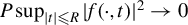


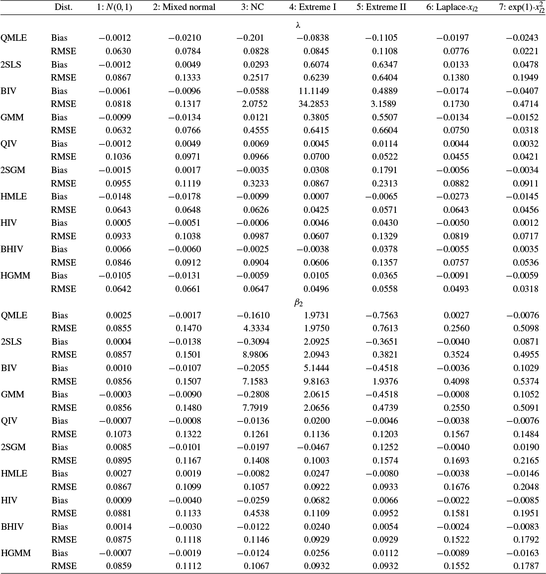

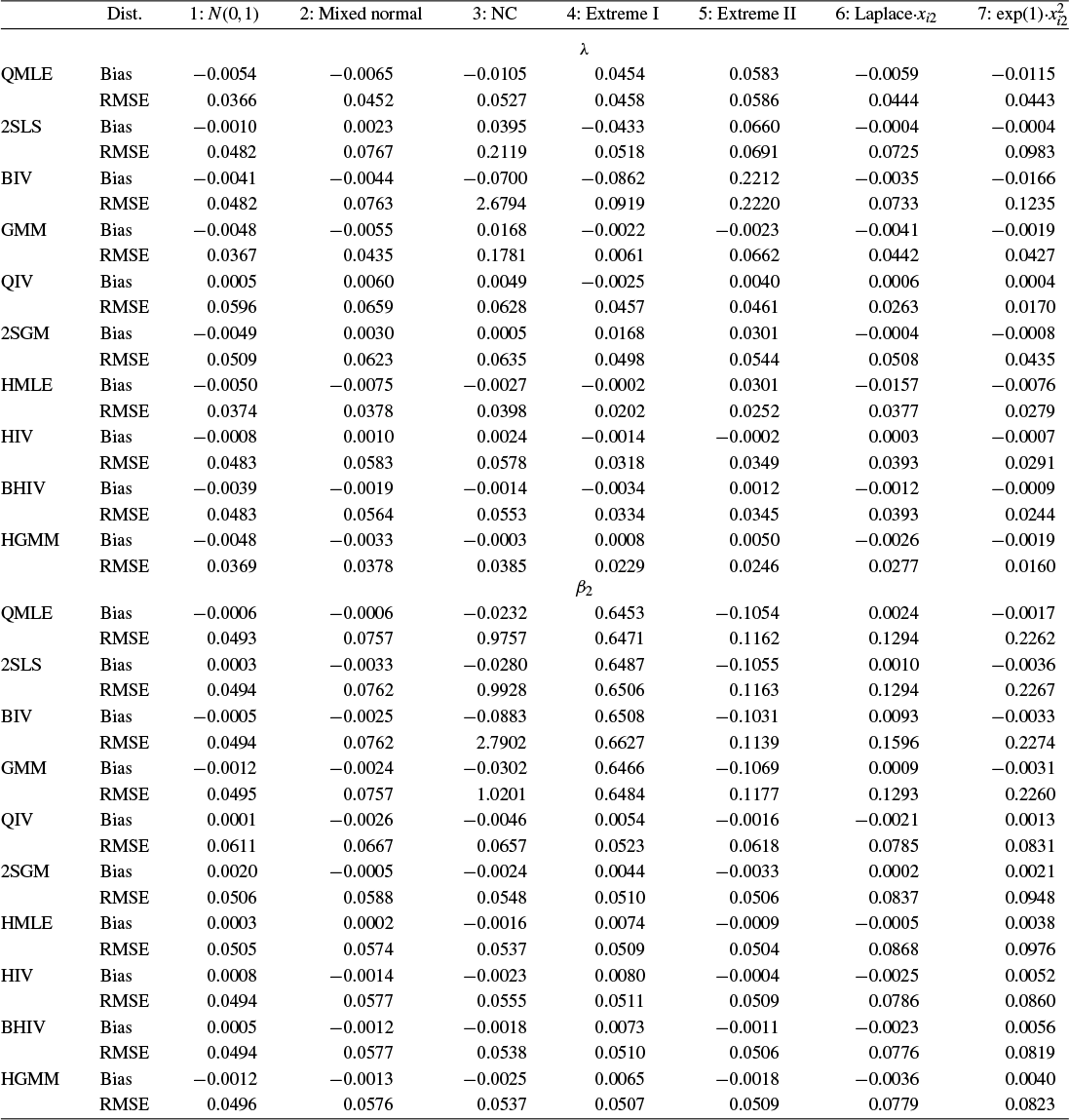

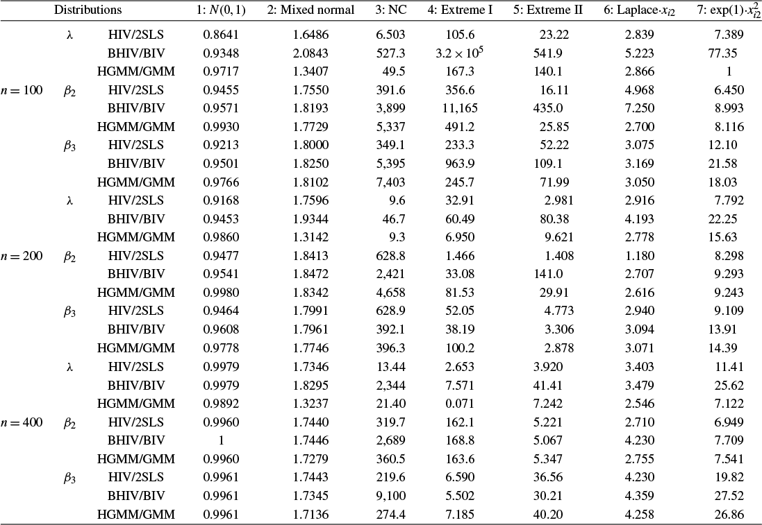
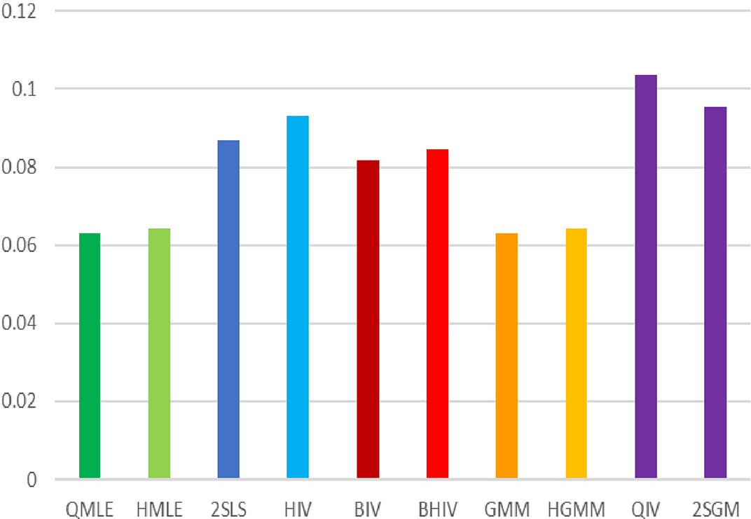


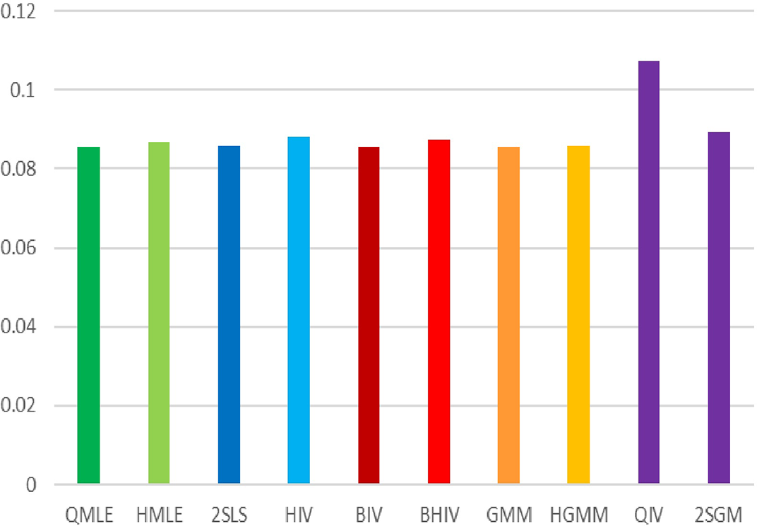


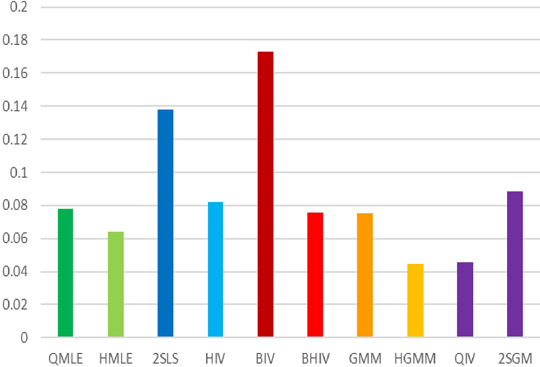


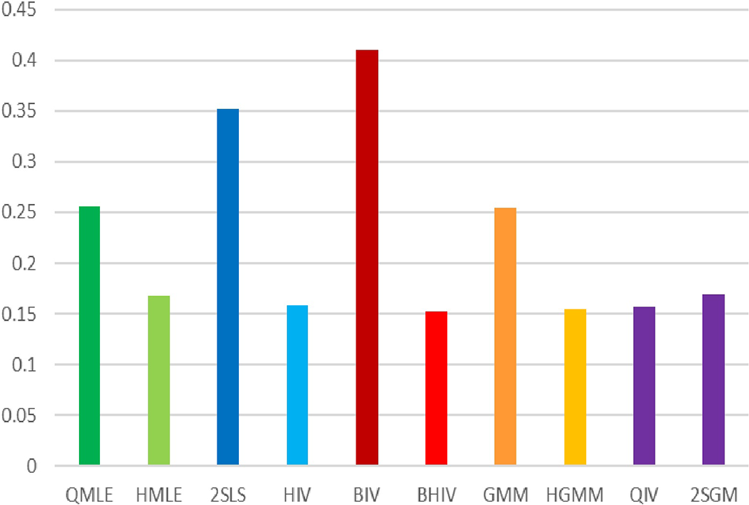


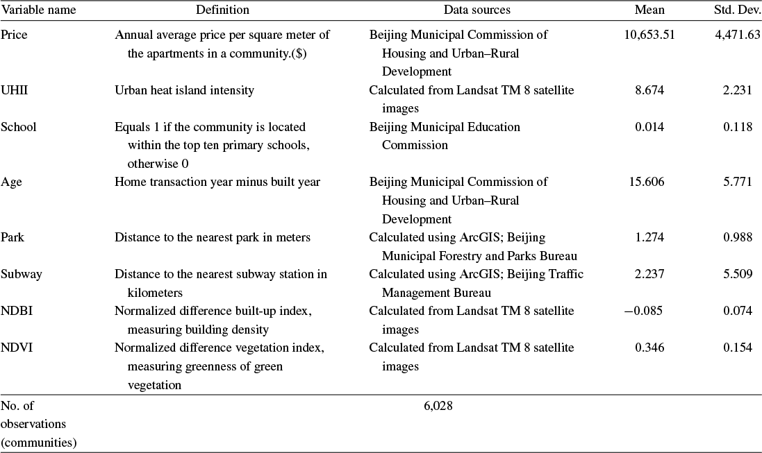
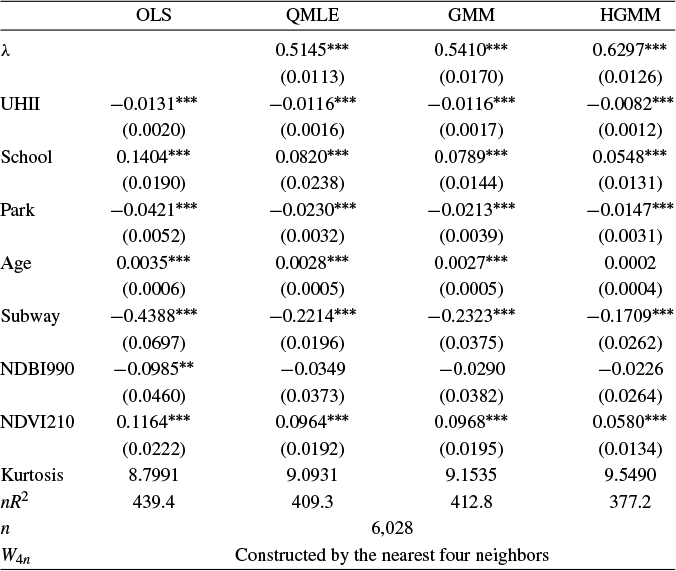


 Open access